A bagging and importance sampling approach to Support Vector Machines

Abstract

An importance sampling and bagging approach to solving the support vector machine (SVM) problem in the context of large databases is presented and evaluated. Our algorithm builds on the nearest neighbors ideas presented in [12]. As in that reference, the goal of the present proposal is to achieve a faster solution of the SVM problem without a significance loss in the prediction error. The performance of the methodology is evaluated in benchmark examples and theoretical aspects of subsample methods are discussed.

1 Introduction

In the context of pattern recognition, classification methods focus on learning the relationship between a set of feature variables and a target “class variable” of interest. From a set of training data points with known associated class labels, a classifier is adjusted, to be used on unlabeled test instances. The diversity of problems that can be addressed by classification algorithms is significant and covers many domains of application (see, for instance, [8] or [20]). More formally, in the setting of supervised learning, examples are given that consist of pairs, $(X_{i},y_{i})$, $i\leq n$, where $X_{i}$ is the $d-$dimensional “feature” or “covariate” vector and $y_{i}$ is the corresponding “class” or “category”, that lives in some finite set ${\cal C}$. Frequently, as in the present work, ${\cal C}$ is assumed to consist only of two classes, labeled $1$ and $-1$.

In recent decades, diverse non-linear procedures have been considered for the classification problem. These techniques have been reported to have a superior performance, in many important problems, with respect to their classical linear counterparts. Among the main non- linear methods, one should mention Classification and Regression Trees (CART) and its general version, Random Forest, Neural Networks, Nearest Neighbor Classifiers, Support Vector Machines (SVM) and probabilistic methods. For detailed accounts of these methodologies, the reader can consult [8], [9], [10], [17], [15], [20] and [14].

Support Vector Machines is a widely used approach in classification, introduced by Boser, Guyon and Vapnik [7], combining ideas from linear classification methods, Optimization and Reproducing Kernel Hilbert Spaces. (See also [13] and [14] for details). The success of SVM in terms of classification error in a variety of contexts, can be explained, in part, by their flexibility. The method uses a kernel function as inner product of “new” feature variables that come from a transformation of the original covariates. Another reason for the success of this methodology is the effort that has been invested in developing efficient methods of solution, some of which, we will discuss below.

With the notation given above for the training data, the soft margin $L^{1}$ classifier SVM problem is stated as

$$\begin{array}[]{ll}\underset{w,b,\xi}{\mbox{minimize}}&\frac{1}{2}\|w\|^{2}+C\sum_{i=1}^{n}\xi_{i}\\ {\rm subject}\;{\rm to}&y_{i}(w^{t}\phi(X_{i})+b)\geq 1-\xi_{i},\;\;\forall\;i=1,...,n,\\ &\xi_{i}\geq 0\end{array}$$ (1)

where $\phi(\cdot)$ is the transformation of the feature vector into a higher dimensional space induced by the use of a kernel function, $C$ is a positive constant that expresses the cost of loosing separation margin or misclassification. The $\xi_{i}$ are the slack variables. The $L^{2}$ version of the soft margin classifier is obtained by replacing the objective function by

$$\frac{1}{2}\|w\|^{2}+C\sum_{i=1}^{n}\xi^{2}_{i}$$

in (1). The dual problem corresponding to (1) can be written as

$$\begin{array}[]{ll}\underset{\alpha}{\mbox{maximize}}&\sum_{i=1}^{n}\alpha_{i}-\frac{1}{2}\sum_{i,j=1}^{n}y_{i}y_{j}\alpha_{i}\alpha_{j}K(X_{i},X_{j})\\ {\rm subject}\;{\rm to}&\sum_{i}y_{i}\alpha_{i}=0,\\ &0\leq\alpha_{i}\leq C\;\;\;\mbox{for}~{}i=1,\ldots,n.\end{array}$$ (2)

where $K(\cdot,\cdot)$ is the kernel function associated to the transformation $\phi$, that is, $K(x,z)=\left\langle\phi(x),\phi(z)\right\rangle$. In the dual problem for the soft margin $L^{2}$ problem, the last restriction in (2), $\alpha_{i}\leq C$, does not appear. This fact simplifies the theoretical analysis presented below in the $L^{2}$ case. The classifier corresponding to the solution of (2) is

$$\mbox{class}(x)=\mbox{sgn}\left(\sum_{i}y_{i}\alpha_{i}^{*}K(X_{i},x)+b^{*}\right).$$ (3)

The estimated prediction error for a given data set is the percentage of points from a test set that are incorrectly predicted. Let us notice that $\alpha_{i}^{*}$ values greater than zero are the only ones that matter for the classifier. The corresponding feature vectors $X_{i}$ are the so-called support vectors. Low cost ways of finding or approximating these vectors is a key issue addressed in the present article.

From the computational viewpoint, solving the convex quadratic program given by (2) can be demanding when the data set is large. A good part of the SVM literature is devoted to finding efficient ways to solve this problem. Some of the ideas that have emerged as a result have to do with solving appropriate sub-problems. In this direction, Osuna et al. [27] introduce a decomposition algorithm in which the original quadratic programming problem is replaced by a sequence of problems of smaller size. An initial working set is considered and data are discarded from the working set or included from the remaining data depending on conditions of optimality. This method relates to the “chunking” methodology as explained in [37] and to the SVM^light algorithm of Joachims [24].

The Sequential Minimal Optimization (SMO) method of Platt [28] is a fairly successful proposal along the line of working with smaller subproblems. In SMO the optimization problem in (2) is solved for two of the $\alpha_{i}$ multipliers at a time, a simplification that allows a closed form solution for each step. In a different direction, Mangasarian and Musicant [25] consider the application of Succesive Overrelaxation (SOR), a method developed originally to solve symmetrical linear complementarity and quadratic programs in order to obtain the solution of the SVM problem.

More in the spirit of identifying the support vectors of the training sample, therefore reducing the training set size, the proposal by Almeida et al[4] applies the $k$-means clustering algorithm to the training set and evaluates the resulting clusters for homogeneity. If a cluster is relatively pure (most observations coming from a single class), its data are discarded. But if a cluster contains data from different classes, it is assumed that, there are probably support vectors in this cluster. Then the observations in the cluster are used in the reduced training data. Abe and Inoue [1] propose computing a Mahalanobis distance classifier first and use those data points, misclassified by this preliminary procedure, in the reduced training set. This assumes that those misclassified by the Mahalanobis procedure are more likely to be near the boundary separating surface for the classification problem. In [31], [32] and [33] the idea of identifying probable support vectors is developed around neighbor properties. Those feature vectors whose neighbors are mixed, belonging to different classes, as well as their nearest neighbors, are included in the reduced training set.

In this order of ideas, Camelo, González-Lima and Quiroz [12] presented a subsampling and nearest neighbors method in which the support vector set of the solution to the SVM problem for a small subsample is iteratively enriched with nearest neighbors to build a relevant training set significantly smaller than the original training data set. The present work seeks to improve the results in [12] by the use of bagging and importance sampling. The idea is to enrich the subsample with more candidates to support vectors by looking simultaneously in different samples and searching for neighbors according to the intensity of candidates found. Since our proposal is closely related to the one in [12], their method will be described in more detail in the following section.

The rest of this paper is organized as follows. In Section 2, we motivate and describe our approach based on bagging and importance sampling. In Section 3, we report and discuss the results of applying the proposed methodology on benchmark examples. Section 5 contains the proof of theoretical results that support the use of subsampling methods, complementing those presented in [12]. The last section includes some conclusions and remarks.

2 Bagging and importance sampling for support vectors

The proposal in [12], based on subsamples and nearest neighbors, can be summarized in the following steps:

Procedure CGLQ

• Select a random sub-sample consisting of a small fraction of the set of examples.

• Solve the SVM problem in that sub-sample, that is, identify the support vectors for the sub-sample. Denote as $\cal V$ this initial set of support vectors. Evaluate the error of the classifier on a test sample set.

• $\cal V$ is enriched with the $k$-nearest neighbors (of each element of $\cal V$) in the complete sample. $\cal V$ is also enriched with the addition of a new small random subsample of the complete sample. With this new sub-sample, we return to step (ii). The iteration stops when there is no important improvement in the classification error.

As reported in [12], on quite diverse benchmark examples, this procedure achieves a classification error comparable to that corresponding to solving the SVM problem on the (original) complete training sample, with significant savings on computation time.

One interesting feature of the method proposed in [12] is that the methodology is not tied to a particular way of solving the SVM problem on the training data.

On the original idea of [12] one could consider the following modifications:

• The initial sub-sample, in step (i) of procedure CGLQ can be substituted by a number of small sub-samples, solving the SVM problem on each one. In this way, we would have a richer supply of candidates to approximate support vectors. The idea of applying an statistical learning procedure to “bootstrap samples” taken from the original training sample, and then combine the output of those different adjusted predictors, is called bagging and was originally proposed by Breiman (see [9] and [10]). Bagging has been particularly successful in the classification context, specifically when used on CART. In that case, the idea of bagging is called Random Forests, and quite often improves on the performance of a single classification tree. Certainly, a trade off must be established in the present context for the application of bagging. If too many initial samples are considered, a rich set of approximate support vectors will be available, but the savings in computation time could be lost.

• The enriching by nearest neighbors can be improved if a certain “intensity of support vectors by region” can be estimated at each point of interest and a sampling procedure is used that takes this intensity into account in order to sample more heavily in regions where more support vectors should be expected. In Monte Carlo simulation, this type of idea appear in what is called importance sampling. See [18], for instance.

It turns out that, by the use of bagging, the goal of estimating a local intensity of support vectors can be achieved. Our proposal in this direction will be to sample and add (to the original set of support vectors) more sample points in those regions where more support vectors are expected. These ideas are embodied in the following procedure. We slightly part from the usual bootstrap practice, by making our initial small sub-samples disjoint (we are not sampling with replacement as in the original definition of bootstrap). This is done to produce a larger initial set of near support vectors. As in the introduction, the training sample is of size $n$ and is formed by pairs $(X_{i},y_{i})$ of feature vectors and class variables, with $y_{i}\in\{-1,1\}$. Procedure Local sampling SVM

• For a positive integer $L$ and $0<\delta<1$, from the original sample, ${\cal X}$, select $L$ disjoint subsamples ${\cal T}_{i}$, $i=1,\ldots,L$, each of size $n_{S}$, such that $n_{S}=\lfloor\delta n/L\rfloor$, where $\lfloor\cdot\rfloor$ denotes the floor function. We denote as $\mathcal{T}$ the set of observations of all the sub-samples i.e. $\mathcal{T}=\cup_{i=1}^{L}{\cal T}_{i}$. $\mathcal{T}$ represents a fraction $\delta$ of the entire training sample.

• On each subsample ${\cal T}_{i}$, solve the SVM problem, finding the set $\mathcal{V}_{i}$, of support vectors associated to that sub-sample. Let ${\cal V}$ denote the union of these initial support vector sets, i.e. ${\cal V}=\cup_{i=1}^{L}{\mathcal{V}}_{i}$ and let $m$ be the size (cardinality) of ${\cal V}$.

• Let $k=\lfloor\ln m\rfloor$. For each $\nu_{j}\in{\cal V}$, identify its $k$th- nearest-neighbor in ${\cal V}$. Denote this $k$th-nearest-neighbor by $NN_{k}(\nu_{j},{\cal V})$ and denote by $\rho_{j}$ the distance between $\nu_{j}$ and $NN_{k}(\nu_{j},{\cal V})$: $\rho_{j}=\mbox{dist}(\nu_{j},NN_{k}(\nu_{j},{\cal V}))$, where $\mbox{dist}(\cdot,\cdot)$ stands for Euclidean distance. Let $\rho$ denote the median of the radii $\rho_{j}$.

• For a parameter $\beta>0$, let $r=\beta\rho$. Define

  $$\eta_{j}=\frac{\rho_{j}^{-1}}{\sum_{i=1}^{\#{\cal V}}\rho_{i}^{-1}}$$

  Sample a fraction $\eta_{j}$ of the points of ${\cal X}\setminus\cal T$ in the ball with center $\nu_{j}$ and radius $r$. Write ${\cal D}_{j}$ for this random sample.

• Solve the SVM problem for the new sample

  $${\cal V}\cup\left(\cup_{j=1}^{L}{{\cal D}}_{j}\right).$$

Three observations are necessary regarding the procedure just described:

1. In order to explain the way importance sample is approximately implemented in our procedure, let us recall the idea of density estimation by “Parzen windows” (see Section 4.3 in [17] for details, including a proof of consistency). Given an i.i.d. sample, $X_{i},\dots,X_{n}$ in ^d, obtained from a probability distribution that admits a density $f(\cdot)$, for an arbitrary $x\in{}^{d}$ (which could be one of the sample points), if $r_{k}(x)$ denotes the Euclidean distance from $x$ to its $k$-th nearest neighbor in the sample, then the density $f(x)$ is consistently estimated by a constant times the reciprocal of the volume of the $k$-th nearest neighbor ball. This means that $f(x)$ is proportional to $(r_{k}(x))^{-d}$. In our case, we use the distance $\rho_{j}$ between each $\nu_{j}$ and its $k$-th nearest neighbor in ${\cal V}$ to get an estimate of the “support vector density” near $\nu_{j}$. Then we set a fixed radius $r$ and sample in a ball of radius $r$ around $\nu_{j}$ with an intensity proportional to $\rho^{-1}_{j}$. Precise importance sampling would require to sample with an intensity proportional to $\rho^{-d}_{j}$, but preliminary experiments revealed that this “exact” importance sampling would result too extreme in the sense of producing heavy sampling in some regions and almost no sampling in others. For this reason, our sampling is proportional to $\rho_{j}^{-1}$.

2. An important difference with the approach put forward in [12] is that in that approach, the enriching of the set ${\cal V}$ occurs inside the $k$-th nearest neighbor balls, while in the present proposal, we use a common fixed radius and change the sampling intensity at each $\nu_{j}$.

3. The parameter $\beta$ in the procedure just described provides flexibility by allowing the user to vary the radius (and volume) of the balls in which the sampling is performed.

Next, we study the behavior of the Local Sampling procedure applied to some real life problems.

3 Applications in benchmark data

In this section we present a performance evaluation of the methodology proposed on four datasets from the LibSVM library. For the experiments described in this section we have used the statistical software R and the e1071 package. Procedures are run on a computer with Motherboard EVGA Classified SR-2 with two microprocessors @ 2.67 GHz and RAM memory of 48 GB 1333 MHz.

For our experiments we consider the following three kernels for the SVMs:

• Linear: $K(\mathbf{x},\mathbf{x}_{j})=\mathbf{x}_{j}^{T}\mathbf{x}$.

• Polynomial with degree $p$, $p\in\mathbb{N}$: $K(\mathbf{x},\mathbf{x}_{j}$)=$(\gamma\mathbf{x}_{j}^{T}\mathbf{x})^{p}$.

• Radial basis: $K(\mathbf{x},\mathbf{x}_{j})=\exp(-\gamma\|\mathbf{x}-\mathbf{x}_{j}\|^{2})$.

Table 1 displays the description of the datasets tested. These examples cover different ranges with respect to sample size and data dimension.

Dataset	TrainSize	TestSize	Features
COD-RNA	59,535	20,000	8
IJCNN1	49,990	15,000	22
COVTYPE	521,012	60,000	54
WEBSPAM	300,000	50,000	254

Table 1: Datasets description

Section 3.2 encompasses the results obtained for the problems tested using the three different kernels. For each one of them, a description is included on how the Local Sampling Algorithm is applied and three tables are displayed. One of them shows the results obtained when solving the problem using the complete data set. Information on the classification error, number of support vectors and computational time are included. The other two tables show the results obtained when using the Local Sampling approach and the CGLQ algorithm from [12]. Each of these tables contain the percentage of the support vectors found by the subsample procedures that are support vectors for the full dataset and the ratio between the classification errors corresponding to the subsample procedures and the full data set. A value less than one for this quotient indicates an improvement in the error when using the subsample approach. The tables also include the percentage that the computational time for the subsample procedures represents of the running time for the complete data set.

3.1 Parameter Choices

In order to choose the kernel parameters and the cost parameter $C$ for the optimization problem, 10-Fold Cross-Validation was used on a small random sample corresponding approximately to 1% of the full training data. The parameters obtained for each problem and kernel are the ones used in all our tests.

With the parameters $\gamma$ and $C$ chosen, the SVM classifier was fitted on the full training sample, obtaining the number and identity of support vectors, the execution time and the test error.

For the Local Sampling approach we proceeded as follows. For each combination of data set and kernel, a fraction $\delta$ (this $\delta$ depends on the problem) of the training data was selected and divided into $L$ sub-samples. The Local Sampling SVM procedure from the previous section was run initially for a value of $\beta$ equal to 0.1 and repeated, increasing $\beta$ by 0.1 at each iteration until there is no decrease in the classification error. Results for the final value of $\beta$ are reported, except that the evaluation done to search for the optimal value of $\beta$ is included in the execution time reported. We take note of the initial amount of support vectors, which is the cardinality of ${\cal V}$ at the end of step (ii) of the procedure, the number of support vectors at the end of the procedure, the number of these which are support vectors for the problem solved on the full training data set, the generalization error on the test data and the execution times.

This whole procedure is run 10 times, on independently chosen initial samples, in order to report averages of the amounts of interest over independent realizations. The next subsection includes the results obtained for the data sets tested.

3.2 Problems Tested

COD-RNA Dataset

The COD-RNA data set contains data for the detection of non-coding RNA’s on the basis of predicted secondary structure. The data are divided into 59,535 observations in the training set and we consider 20,000 observations in the test sample, each with 8 attributes measuring genetic information.

Table 2 displays the results for the SVM solution considering the full training sample and the optimal parameters $C$ and $\gamma$ obtained in the preliminary evaluation for each of the kernels considered.

Table 2: SVM results from full COD-RNA training data

	Optimal parameters
Kernel	Cost	$\gamma$	Number of Support Vectors	Error rate	Time (s)
Linear	0.1	–	22923 (11462 $||$ 11461)	0.206	178.013
Polynomial	1	0.1	15397 (7698 $||$ 7699)	0.208	114.115
Radial basis	10	0.1	8768 (4380 $||$ 4388)	0.242	117.901

The second and third columns in Table 2 show the optimal parameters obtained by cross validation. The following column shows the number of support vectors found in the solution for each kernel. The quantities in parentheses that follow, indicate the division of these support vectors by class. The error rates obtained in the test set are included in the fifth column. For the polynomial kernel, in this example, the degree used was $p=3$.

In this case, the best performance for the complete data set, in terms of test error, is obtained for the linear and polynomial kernels, which produce very similar errors. The linear kernel solution requires a significantly larger amount (22,923) of support vectors, compared to the other kernels. Execution times in seconds are shown in the sixth column. The polynomial kernel has the best performance in terms of execution time, taking approximately 114 seconds. The higher execution time needed by the linear kernel solution probably correlates with the large number of support vectors this solution requires.

To apply the local sampling SVM scheme to the CODRNA data, we used $\delta=0.01$, dividing the training sample in 12 subsamples of size 50. With the optimal parameters chosen and for each of the three kernels, we executed 10 runs of the algorithm proposed as described above. Table 3 shows the results for our methodology compared with the results obtained using the methodology proposed in [12]. As pointed out before the results are shown only for the final value of $\beta$.

Table 3: COD-RNA error and computing times vs CGLQ algorithm

COD-RNA	Kernel
	Linear	Polynomial	Radial basis
$\beta$	0.1	0.1	0.1
SV initial	395	442	362
SV final	1296	1293	585
SV real	1127	757	338
% full SV	4.91 %	4.91%	3.85 %
Error rate	0.21	0.19	0.24
Sd. dev.	(0.02)	(0.007)	(0.01)
Error ratio	1.02	0.92	1.01
Time (s)	1.1095	1.3719	0.8647
% full time	0.62 %	1.2 %	0.73 %

(a) Local Sampling SVM

COD-RNA	Kernel
$\delta$=0.01, $K$=5	Linear	Polynomial	Radial basis
SV initial	272	320	193
SV final	3417	2945	1695
SV real	3332	2203	1184
% full SV	14.53 %	14.3 %	13.51 %
Error rate	0.2068	0.193	0.24
Sd. dev.	(0.005)	(0.005)	(0.01)
Error ratio	1.004	0.92	1.01
Time (s)	5.08	4.89	5.03
% full time	2.85 %	4.29 %	4.26 %

(b) CGLQ Algorithm

In Table 3 we observe the following: The method proposed in [12] finds a significantly larger number of complete sample support vectors, in comparison with the local sample procedure proposed here. Still, in terms of test errors the results for the method of [12] and our local sample scheme are very similar and both are quite successful, with error ratios very close to 1 for all the kernels. The main difference between the two methods compared lie, in this example, in the execution time. For all kernels, the method proposed here requires between 20% and 25% of the computing time in comparison to the algorithm of [12] (that was already very efficient in terms of computing time).

IJCNN1 Dataset

The IJCNN1 data set was used in the 2001 Neural Network Competition, and contains information on a time series produced by a physical system. It consists of 49,990 observations in the training sample and we use 15,000 observations for testing. The number of features is 22.

For this data set, the degree used for the polynomial kernel was $p=3$. The results obtained for the SVM problem on the complete training data set using the estimated optimal parameters are shown in Table 4.

Table 4: SVM results from full IJCNN1 training data

	Optimal parameters
Kernel	Cost	$\gamma$	Number of Support Vectors	Error rate	Time (s)
Linear	5	–	8577 (4296 $||$ 4281)	0.078	63.99
Polynomial	0.1	0.5	9377 (4706 $||$ 4631)	0.071	62.5
Radial basis	10	0.1	5731 (2877 $||$ 2854)	0.028	63.45

On this example, the execution times on the complete data set are very similar for the three kernels. In terms of test error, the best performance is obtained with the radial basis kernel, reaching an error rate of 2.8 %.

In this case, the local sampling SVM approach is used with 20 subsamples of size 50, corresponding to a value of $\delta$ equal to 0.02. Tables 5(a) and 5(b) summarize the results on the IJCNN1 for the Local Sampling procedure and the CGLQ method.

IJCNN1	Kernel
	Linear	Polynomial	Radial basis
$\beta$	0.2	0.2	0.2
SV initial	347	503	395
SV final	834	407	1055
SV real	711	317	610
% full SV	8.29 %	3.38 %	10.64 %
Error rate	0.069	0.06	0.028
Sd. dev.	(0.002)	(0.008)	(0.001)
Error ratio	0.89	0.85	1.02
Time (s)	1.98	2.18	6.23
% time SVM	3.09 %	3.48 %	9.82 %

(a) Local Sampling SVM

IJCNN1	Kernel
$\delta$=0.02, $K=$5	Linear	Polynomial	Radial basis
SV initial	180	263	197
SV final	673	295	394
SV real	607	235	234
% full SV	7.07 %	2.5 %	4.09 %
Error rate	0.068	0.07	0.036
Sd. dev.	(0.005)	(0.01)	(0.0008)
Error ratio	0.87	1.08	1.29
Time (s)	2.5	0.77	2.98
% time SVM	3.68 %	1.23 %	4.78 %

(b) Camelo et al. Algorithm

Table 5: IJCNN1 error and computing times

Table 5(a) shows that, for the IJCNN1 data set, the local sampling scheme finds a larger fraction of the full data support vectors, in comparison to the procedure of [12]. Both methods perform very well and similarly in terms of test error for the Linear and Polynomial kernels. For the Radial Basis kernel, which was the kernel with the smallest error on the complete sample, the performance of local sampling is better, keeping the error ratio near 1. This comes at the cost of doubling the execution time of procedure CGLQ, but still keeping the execution time under 10% of that for the full data set.

COVTYPE Dataset

The Covertype data set contains information for predicting forest cover type from seven cartographic variables. In this case, we considered a modified version that converts a seven class problem into a binary classification problem, where the goal is to separate class 2 from the other 6 classes. The number of instances is 581,012 and each instance is described by 54 input features. For our implementation we consider 521,012 observations in the training set and 60,000 instances for testing.

For this data set, the degree used for the polynomial kernel was $p=2$. Table 6 shows the results of solving this problem on the complete training data set, for the optimal parameters chosen. For all three kernels, there is a large amount of support vectors, evenly distributed between the two classes. In terms of error, the best performance is obtained with the radial basis kernel with an error rate equal to 9 %. This is a complex problem, for which the best solution takes about eight hours of computation time.

Table 6: SVM results from full COVTYPE training data

	Optimal parameters
Kernel	Cost	$\gamma$	Number of Support Vectors	Error rate	Time (s)
Linear	10	–	303036 (151517 $||$ 151519)	0.237	36688.26
Polynomial	1	1	216841 (108421 $||$ 108420)	0.169	39896.5
Radial basis	10	5	144271 (72113 $||$ 72158)	0.09	28746.54

For the local sampling SVM approach, we used 50 subsamples of size 250, corresponding to a choice of $\delta=$0.025. Tables 7(a) and 7(b) show the comparison of results in this example for the local sampling and the CGLQ method.

In this case, the optimal value of the parameter $\beta$ goes up to 0.5 in order to reach better error rates. This shows the usefulness of a flexible parameter $\beta$ in complex problems. The local sampling procedure identifies as support vectors a large fraction (about 40%) of the support vectors for the complete problem. The error rates achieved by both methods compared are very good and quite similar. The main difference in performance is again in the execution times, which are significantly smaller for the local sampling procedure.

COVTYPE	Kernel
	Linear	Polynomial	Radial basis
$\beta$	0.5	0.5	0.5
SV initial	7779	7208	10785
SV final	139747	96003	72188
SV real	136108	87888	63103
% full SV	44.91 %	40.53%	43.73 %
Error rate	0.2391	0.1789	0.11
Sd. dev.	(0.0008)	(0.0006)	(0.001)
Error ratio	1.009	1.05	1.22
Time (s)	6531.96	7928.2	7932.9
% time SVM	17.8 %	19.87 %	27.59 %

(a) Local Sampling SVM

COVTYPE	Kernel
$\delta$=0.05, $K=$5	Linear	Polynomial	Radial basis
SV initial	15226	11974	10603
SV final	76972	55204	37049
SV real	76307	40306	21153
% full SV	25.18 %	18.58%	14.66 %
Error rate	0.23	0.17	0.11
Sd. dev.	(0.00002)	(0.0009)	(0.01)
Error ratio	0.99	1.02	1.22
Time (s)	11424.73	13343.96	8887.25
% time SVM	31.14 %	33.44 %	30.91 %

(b) Camelo et al. Algorithm

Table 7: COVTYPE error and computing times

WEBSPAM Dataset

The Webspam data set is a collection of 350,000 webspam pages that were obtained using an automatic methodology. We consider the set used in the Pascal Large Scale Learning Challenge with the normalized unigram data set that contains 254 features. In our implementation, we split the data into two sets: training set with 300,000 observations and testing set with 50,000 observations.

The parameters $\gamma$ and $C$ were found as in the previous problems by using cross validation. The polynomial kernel was considered with degree $p=3$. Table 8 shows the results for the solution of this problem on the complete training data. It appears that this is a problem in which the SVM methodology works well, in the sense that very low error rates are obtained, being the minimum test error of 1.1%, obtained with the radial basis kernel. The linear kernel is probably the least convenient for this problem, since it produces the largest error rate with the highest computing time.

Table 8: SVM results from full WEBSPAM training data

	Optimal parameters
Kernel	Cost	$\gamma$	Number of Support Vectors	Error rate	Time (s)
Linear	10	–	56810 (28407 $||$ 28403)	0.068	21917.83
Polynomial	10	2	16789 (8541 $||$ 8248)	0.014	16492.46
Radial	10	2	16623 (8748 $||$ 7875)	0.011	10972.71

For this data set, when the Local Sampling approach was used, it was necessary to choose a value of $\delta=0.1$ in order to obtain an approximation close enough to the best solution. For this value of $\delta$, 25 subsamples of size 1400 were used. Table 9(a) summarizes the results on this data set for the Local Sampling procedure.

WEBSPAM	Kernel
	Linear	Polynomial	Radial basis
$\beta$	0.5	1	1
SV initial	9341	6083	7499
SV final	35155	10141	13030
SV real	32182	8755	9049
% full SV	56.46 %	52.04 %	54.46 %
Error rate	0.069	0.0178	0.018
Sd. dev.	(0.0004)	(0.0005)	(0.0004)
Error ratio	1.02	1.27	1.63
Time (s)	3931.96	3491	3683.11
% time SVM	17.93 %	21.16 %	33.56 %

(a) Local Sampling SVM

WEBSPAM	Kernel
$\delta$=0.10, $K$=10	Linear	Polynomial	Radial basis
SV initial	6358	2770	3474
SV final	31791	7764	10337
SV real	29793	6208	6444
% full SV	52.44 %	36.97%	38.76 %
Error rate	0.068	0.0169	0.017
Sd. dev.	(0.0004)	(0.0004)	(0.0002)
Error ratio	1.005	1.21	1.55
Time (s)	7318.467	3396.78	2314.489
% time SVM	33.39 %	20.59 %	21.09 %

(b) Camelo et al. Algorithm

Table 9: WEBSPAM error and computing times

Figure 1 shows the evolution of the estimated error for the Local Sampling solution of the WEBSPAM problem, as a function of $\delta$. The dotted green and blue lines show, respectively, the largest and smallest errors achieved with the Local Sampling methodology, while the dotted red line corresponds to the estimated error for the solution for the whole data set.

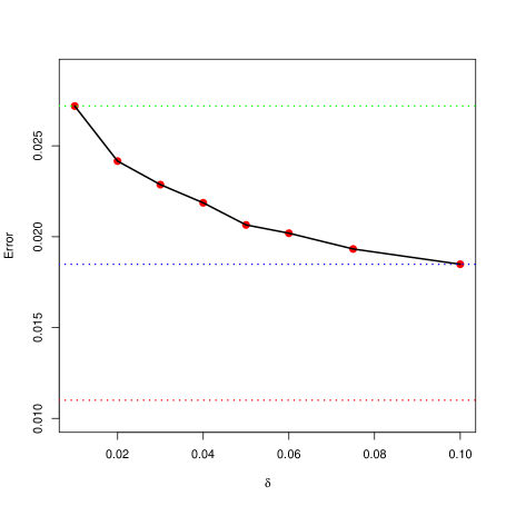
Figure 1: Classification error vs $\delta\in[0.01,0.1]$ for the Local Sampling SVM procedure- WEBSPAM problem.

Table 9(b) summarizes the results obtained with the CGLQ methodology. Comparing both subsample approaches for this example we find that, for the linear Kernel, the Local Sampling approach is better than CGLQ since it obtains similar error with a much lower computational time. And this error is almost the same as the one obtained for the whole data set. For the polynomial kernel, similar performances were found. However, for the radial basis kernel, the best results are obtained with the CGLQ algorithm, in terms of the generalization error and the execution time. However, it should be highlighted that in this problem, for the nonlinear kernels, the classification errors reached by any of the subsample procedures are, in terms of the error ratio, the worst among all the tested examples. We believe that this performance is due to the detrimental effect that may have the high dimensions of the data when using these type of approaches, as our theoretical results suggest. This will be discussed in Section 4.

3.3 Practical Remarks

In this subsection we would like to summarize our findings regarding the parameter choices ($\delta$, $L$, and $\beta$) for the Local Sampling procedure, which could serve as guidelines for its use.

The size of each subsample is determined by the value of the parameter $\delta$. We conclude, from our experimentation, that for problems with data set of medium size, this is, size of order around $10^{5}$ and $10^{6}$, and low dimension (dimension less than 30), the values of delta should be chosen between $1\%$ and $5\%$. This can be implemented by starting from $\delta=1\%$ and sequentially increasing the value, depending on the improvement in the error and the execution times. For problems with larger training sample size in higher dimension, consider using larger values of delta, up to $10\%$.

The number of subsamples, $L$, to be chosen depends on the value of $\delta$ and the complete data set size. If the number of points at each subsample is too small, this is, that there is poor information about the full population inside the subsamples, a large number of these points will become support vectors of the corresponding SVM problems and they will not contribute to approximate the real ones for the complete data set. Therefore, $L$ is chosen trying to get a balance between the number of observations defined by the $\delta$’s and the distribution of these observations in the subsamples, in such a way that the number of points at each subsample is not too small. We want to get a reasonable amount of support vectors for each subproblem that provide valuable information for the next step.

Regarding the choice of the parameter $\beta$, our experience indicates that values in the interval $[0.1,0.5]$ are useful, in terms of including enough information from the sample. Increasing beta will improve the performance in terms of validation error at the cost of larger execution time. A guideline could be to start with $\beta=0.1$ and repeat with increments of $0.1$ while there is a significant improvement in classification error or until a limit is reached in terms of execution time.

Next we will present our theoretical results.

4 Theoretical results

The purpose of the present section is to establish a stability result for the solution of the soft margin $L^{1}$ SVM problem, that can shed some light on the performance of subsampling schemes as the one proposed in the preceding sections.

Using the notation established in Section 1, here we consider an i.i.d. sample of pairs $(X_{i},y_{i})$ for $i=1,\dots n$, where the $X_{i}$ follow a probability distribution $\mu$ on ^d, the $y_{i}$ take the values $1$ and $-1$ and, given $X_{i}=x$, the distribution of $y_{i}$ is given by $\Pr(y_{i}=1\,|\,x)=\eta(x)$ for a measurable function $\eta$ on on the support of $\mu$.

We assume that $\mu$ admits a density $f$ with respect to Lebesgue measure, $\lambda$, which is bounded away from zero and infinity on its compact support, $\cal S$. Also, we assume that $\eta$ (at least in the vicinity of support vectors), is bounded away from 0 and 1.

A random subsample, $\cal M$, is taken, of size $n^{\prime}=\lceil\delta n\rceil$ for some $\delta>0$. Based on this subsample, the SVM problem is solved and our purpose is to quantify the similarity of the solution obtained with ${\cal M}$ to the one given by (3), in which the whole data set is employed. In what follows, the expression with high probability, means that the probability of the event considered goes to 1, as $n\to\infty$.

Let ${\cal V}_{n}$ the set of support vectors for the SVM solution computed with the complete sample of size $n$ and let $q$ be its cardinal, i.e. $q=\#{\cal V}_{n}$, the number of support vectors. The first thing to be verified is that with high probability, the subsample $\cal M$ will contain points close enough, say, to a distance less than $\rho$, of each point $X_{i}$ in the distinguished set ${\cal V}_{n}$, for any $\rho$ such that $\rho^{d}$ is of order $\mathrm{O}(\textrm{ln}^{2}n/n)$.

Besides the assumptions on the sample distribution stated above, we will assume the following shape condition on $\cal S$, called weak grid compatibility, which is a relaxed version of a condition considered in [11], in the context of theory of clustering algorithms.

Definition 1

Let $\cal S$, as above, denote the support of the density $f$ generating the data. We will say that $f$ and $\cal S$ satisfy the weak grid compatibility condition, if there is a positive number $\gamma$, such that for all small enough $l>0$, $\cal S$ can be covered, possibly after translation and rotation, by a regular array $\cal W$, of cubes of side $l$, such that:

$$\forall V\in{\cal W},\lambda(V\cap{\cal S})\geq\gamma\lambda(V),$$

where $\lambda$ denotes Lebesgue measure in $\mathbb{R}^{d}$ and regular array of cubes in $\mathbb{R}^{d}$ means that the vertices of the cubes form a regular grid in $\mathbb{R}^{d}$, in the sense that the length between the contiguous vertices is constant and equal to $l$. In this definition it is assumed that $\cal W$ includes only the cubes needed to cover $\cal S$, that is, if $W\cap{\cal S}=\emptyset$ the $W\notin\cal W$. According to [11], $d$-dimensional balls and ellipsoids in $\mathbb{R}^{d}$ as well as regular polyhedra satisfy this condition.

As a condition on the kernel $K(\cdot,\cdot)$ employed in the SVM procedure, we assume that $K$ is Lipschitz continuous, with Lipschitz constant $L$.

Finally, we make assumptions on the solution of the soft margin problem (1) on the whole data set. First we assume the following asymptotic continuity condition on the uncertainty of the classification function for the solution of the SVM problem on the complete data set: Let $\alpha_{i}^{*}$ and $b^{*}$ be the solution coefficients appearing in (3). We assume that

$$\lim_{\epsilon\to 0}\,\limsup_{n}\mu\left(x\in{\cal S}:\left|\sum_{i}y_{i}\alpha_{i}^{*}K(X_{i},x)+b^{*}\right|\leq\epsilon\right)=0,a.s.$$ (4)

where the expression “almost surely” refers to the product space of infinite samples. Condition (4) is bounding the level of uncertainty that the solution to the SVM problem admits. Points $x\in\cal S$ for which the condition

$$\left|\sum_{i}y_{i}\alpha_{i}^{*}K(X_{i},x)+b^{*}\right|\leq\epsilon$$

holds, are points near the boundary of indecision of the SVM solution. We are asking that, as $\epsilon$ becomes smaller, this region of $\epsilon$-uncertainty has probability that goes to zero. Simulations shown in Subsection 4.2 suggests that condition (4) holds comfortably in real examples.

The last assumptions, on the other hand, are technical and more restrictive assumptions on the number of support vectors that the solution associated to the complete data set might have. On one hand, we suppose that the cardinality $q$ of the set ${\cal V}_{n}$ of support vectors is $\mbox{o}_{\Pr}\Big{(}\Big{(}\frac{n}{\textrm{ln}^{2}n}\Big{)}^{1/d}\Big{)}$, namely, for each $\epsilon>0$,

$$\Pr\left(q>\epsilon\left(\frac{n}{\textrm{ln}^{2}n}\right)^{1/d}\right)\rightarrow 0,\>\>\mbox{ as }\>\>n\rightarrow\infty.$$ (5)

The power $1/d$ in this bound, makes the condition more restrictive in large dimensions, reflecting the “curse of dimensionality” that appears frequently in the pattern recognition literature. In addition to (5), we also need to bound the amount of support vectors that the solution for the soft margin $L^{1}$ problem can have in a small cube. Assume that, when the sample size is $n$, $\cal S$ is covered (by weak grid compatibility), with a regular array ${\cal W}_{n}$ such that each cube $V\in{\cal W}_{n}$ has sides of length

$$l=l_{n}=\kappa(\textrm{ln}^{2}n/n)^{1/d}$$

for some positive constant $\kappa$. We assume that there exists a constant $C_{1}$

$$\Pr(\max\,\{\#\left({\cal V}_{n}\cap V\right):V\in{\cal W}\,\}>C_{1})\rightarrow 0,\>\>\mbox{ as }\>\>n\rightarrow\infty,$$ (6)

where, again, ${\cal V}_{n}$ is the set of support vectors for the solution of the SVM problem. Although neither of the two last conditions implies the other, (5) is, by far, more restrictive than (6) on the total number of support vectors that the problem might admit, since the second condition does not reflect the curse of dimensionality. Condition (6) imposes a sublinear limit on the number of support vectors that can appear in any particular small neighborhood.

As a first result we prove that for a subsample of size $\lceil\delta n\rceil$, with high probability, there will exist in the subsample, observations with labels of both classes, close to the support vectors of the complete sample solution. Since the support vectors delimit the surface that separates the two classes, it is natural to expect that in a neighborhood of each support vector, points from both classes are to be found, even in a subsample.

Proposition 1

Under the setting described above, there exists a $\rho=\rho(n)$, which is of the order $\mathrm{O}((\textrm{ln}^{2}n/n)^{1/d})$ such that for each $X_{i}\in{\cal V}_{n}$ there are $X_{i^{\prime}}\in\cal{M}$ with $Y_{i^{\prime}}=1$ and $X_{i^{\prime\prime}}\in\cal{M}$ with $Y_{i^{\prime\prime}}=-1$ such that

$$\|X_{i}-X_{i^{\prime}}\|\leq\rho\quad\text{y}\quad\|X_{i}-X_{i^{\prime\prime}}\|\leq\rho$$

Proof: From the assumptions, there are positive constants $a_{1}$ and $a_{2}$, such that $0<a_{1}\leq f(x)\leq a_{2},\forall x\in\cal S$ and $b_{1}$ and $b_{2}$, such that $0<b_{1}\leq\eta(x)\leq b_{2}<1$. By the grid compatibility assumption, there exists a cover of $\cal S$, $\cal W$, composed of cubes $E_{n,j}$ of side $\mbox{O}\left(\left(\frac{\textrm{ln}^{2}n}{n}\right)^{\frac{1}{d}}\right)$. The volume of each cube is of the order $\mbox{O}\left(\frac{\textrm{ln}^{2}n}{n}\right)$.

By weak grid compatibility, there exists a positive $\gamma$ such that, for each $j$

$$\mu(E_{n,j})=\mu(E_{n,j}\cap{\cal S})\geq\gamma a_{1}\frac{\textrm{ln}^{2}n}{n}.$$ (7)

Let

$$B_{n,j}=E_{n,j}\times\{1\}\qquad\mbox{and}\qquad{\cal N}^{+}_{n,j}=\#\{(X_{\ell},y_{\ell})\in B_{n,j}\cap{\cal M}\}$$

${\cal N}^{+}_{n,j}$ is the number of observations of the subsample $\cal M$, in $E_{n,j}$, whose class is 1. Also, define

$$p_{n,j}=\text{Pr}((X,y)\in B_{n,j}),$$

where $(X,y)$ is a new pair produced by the same random mechanism generating the sample. The distribution of ${\cal N}^{+}_{n,j}$ is binomial with parameters $n^{\prime}=\lceil\delta n\rceil$ and $p_{n,j}$ i.e. ${\cal N}^{+}_{n,j}\sim\text{Bin}(n^{\prime},p_{n,j})$ and, by our assumptions, $\gamma a_{1}b_{1}\textrm{ln}^{2}n/n\leq p_{n,j}\leq\gamma a_{2}b_{2}\textrm{ln}^{2}n/n$. Then, the probability of finding no subsample observations in $E_{n,j}$, for a fixed $j$, is

$$\text{Pr}\Big{(}{\cal N}^{+}_{n,j}=0\Big{)} \leq\text{Bin}(n^{\prime},p_{n,j})(0)$$

$$\leq\textrm{exp}\Bigg{\{}-\delta\gamma a_{1}b_{1}{\textrm{ln}^{2}n}\Bigg{\}}$$

$$=n^{-\delta\gamma a_{1}b_{1}\textrm{ln}n}.$$

Notice that by (7), we have

$$\#{\cal W}\leq\frac{n}{\gamma a_{1}\textrm{ln}^{2}n},$$ (8)

It follows that the probability of having no points of the subsample of class 1 in some of the cubes in $\cal W$ can be bounded as

$$\text{Pr}\Big{(}\cup_{j}\{{\cal N}^{+}_{n,j}=0\}\Big{)} \leq\frac{n}{\gamma a_{1}\textrm{ln}^{2}n}\text{Pr}\Big{(}{\cal N}^{+}_{n,j}=0\Big{)}$$ (9)

$$\leq\frac{n}{\gamma a_{1}\textrm{ln}^{2}n}\cdot n^{-\delta\gamma a_{1}b_{1}\textrm{ln}n}$$

$$=\frac{1}{\gamma a_{1}\textrm{ln}^{2}n}n^{1-\delta\gamma a_{1}b_{1}\textrm{ln}n}.$$

Since the bound on the right hand side of (9) summed over $n$, adds to a finite value, we get, by Borel-Cantelli, that the event: “There exists a cube in $\cal W$ that contains no points of the subsample of class 1” will not occur, for large enough $n$, almost surely. In other words

$$\text{Pr}\Big{(}\limsup_{n}\cup_{j}\{{\cal N}^{+}_{n,j}=0\}\Big{)}=0$$ (10)

The version of (10) for subsample points with $y_{i}=-1$ is obtained similarly. Since every support vector in ${\cal V}_{n}$ must fall in a $E_{n,j}$, for some $j$, the result follows. $\square$

The assumptions in Proposition 1 may seen too restrictive, in asking that both $f$ and $\eta$ be bounded away from extreme values on the whole domain $\cal S$. Those requirements could be weakened, by requiring those conditions to hold only in regions of $\cal S$ where support vectors might appear. Then, the argument in the proof would not consider all cubes in $\cal W$, but only the collection ${\cal E}=\{E_{n,j}\in{\cal W}:{\cal V}_{n}\cap E_{n,j}\neq\emptyset\}$, that is, those cubes in the grid that contain support vectors.

4.1 Stability of the SVM solution

The following theorem is stated in the context of the soft margin $L^{1}$ SVM problem. The corresponding result for the soft margin $L^{2}$ version of the problem also holds, and is easier to prove in that case.

Theorem 1

Fix $\epsilon$ greater than 0. Let $\alpha^{*}_{i}$ and $b^{*}$ be the multipliers appearing in (3) for the solution of the SVM problem associated to the complete training data set. There exists a constant $M\geq 1$, such that
(i) If we replace $\alpha^{*}_{i}$ and $b^{*}$ by $\gamma^{*}_{i}=\alpha^{*}_{i}/M$ and $c^{*}=b^{*}/M$ in (3), the new set of coefficients continue to be feasible for the problem (2) and the two corresponding classifiers (with the original coefficients and the coefficients divided by $M$) coincide, that is, produce always the same classification on new data points.
(ii) For the soft margin $L^{1}$ problem on the subsample ${\cal M}$, there exist multipliers $\beta^{*}_{\ell}$, feasible for the problem (2) on ${\cal M}$, such that, with high probability,

$$\Big{|}\sum_{i}y_{i}\gamma^{*}_{i}K(X_{i},x)-\sum_{\ell}y_{\ell}\beta^{*}_{\ell}K(X_{\ell},x)\Big{|}<\epsilon\qquad\mbox{for all }\>x\in{\cal S},$$ (11)

where the $(X_{\ell},y_{\ell})$ are the data points in $\cal M$.
(iii) Let class${}_{\,\mbox{full}}(x)$ be the classifier defined by (3) and obtained from the solution of the $L^{1}$ soft margin SVM problem for the complete sample and class${}_{\mbox{sub}}(x)$ the classifier defined by

$$\mbox{class}_{\mbox{sub}}(x)=\mbox{sgn}\left(\sum_{\ell}y_{\ell}\beta^{*}_{\ell}K(X_{\ell},x)+c^{*}\right)$$ (12)

Then, with high probability,

$$\mu\left(x\in{\cal S}:\mbox{class}_{\,\mbox{full}}(x)\neq\mbox{class}_{\mbox{sub}}(x)\right)<\epsilon$$ (13)

Proof:

Let $B$ be the set of probability 1 where (10) holds. We assume that our sample,
$(X_{1},y_{1}),(X_{2},y_{2}),\dots$ falls in that set. Consider the cube array, $\cal W$, of the previous proposition and the subcollection ${\cal E}=\{E_{n,j}\in{\cal W}:{\cal V}_{n}\cap E_{n,j}\neq\emptyset\}$ of cubes where the solution of the SVM problem for the complete sample of size $n$ has support vectors. Let $j$ be such that $E_{n,j}\in{\cal E}$. Define

$$A^{+}_{n,j}=\{i\leq n:\alpha^{*}_{i}>0,X_{i}\in E_{n,j}\mbox{ and }y_{i}=+1\},$$

$$A^{-}_{n,j}=\{i\leq n:\alpha^{*}_{i}>0,X_{i}\in E_{n,j}\mbox{ and }y_{i}=-1\},$$

and let

$$s^{+}_{n,j}=\sum_{i\in A^{+}_{n,j}}\alpha^{*}_{i}\qquad\mbox{ and }\qquad s^{-}_{n,j}=\sum_{i\in A^{-}_{n,j}}\alpha^{*}_{i}$$

in the understanding that a sum over the empty set is 0. $s^{+}_{n,j}$ is the sum of the multipliers associated to support vectors with class +1 in the cube $E_{n,j}$. We want to assign the sum of multipliers in the cube as multiplier for a vector of the subsample in $E_{n,j}$. But then, the new set of coefficients could fail to satisfy the upper bound restriction $\alpha_{i}\leq C$ in (2). For that reason, we consider the sets $S^{+}=\{s^{+}_{n,j}/C,j\geq 1\}$ and $S^{-}=\{s^{-}_{n,j}/C,j\geq 1\}$ and $M=\max\left(S^{+}\bigcup S^{-}\bigcup\{1\}\right)$. All the $s^{+}_{n,j}$ and $s^{-}_{n,j}$, divided by $M$ are bounded above by $C$. It is simple to verify that, by defining $\gamma^{*}_{i}=\alpha^{*}_{i}/M$, for each support vector in ${\cal V}_{n}$ and $c^{*}=b^{*}/M$, we obtain a new set of multipliers that satisfies the feasibility conditions (2) and that produce the same classification for each $x\in\cal S$ as the original classifier. Thus, part (i) is proved. As a bonus, we observe that, by assumption (6), $M\leq C_{1}$ for the value of $C_{1}$ appearing in that assumption.

Since we are working in $B$ and the sample is large enough, for each $j$ such that $E_{n,j}\in{\cal E}$, there exists at least one $X_{\ell}\in{\cal M}\cap E_{n,j}$ with $y_{\ell}=+1$. Choose one of those $X_{\ell}$, and assign to it the multiplier

$$\beta^{*}_{\ell}=\sum_{i\in A^{+}_{n,j}}\gamma^{*}_{i}$$ (14)

Define similarly $\beta^{*}_{\ell}$ for a point $X_{\ell}\in{\cal M}\cap E_{n,j}$ with $y_{\ell}=-1$ in terms of the $\gamma^{*}_{i}$ for support vectors in $E_{n,j}$ with $y_{i}=-1$. For the $X_{\ell}$ not chosen, set $\beta_{\ell}=0$. By construction, the set of coefficients $\beta^{*}_{\ell}$ just defined, together with $c^{*}=b^{*}/M$ is feasible as solution associated to $\cal M$.

Now, for each $x\in\cal S$, and the chosen $X_{\ell}\in{\cal M}\cap E_{n,j}$ with $y_{\ell}=+1$, we have, using (14), that $K$ is Lipschitz and that the diameter of $E_{n,j}$ is $\mathrm{O}((\textrm{ln}^{2}n/n)^{1/d})$ by the construction of the previous Proposition,

$$|\sum_{i\in A^{+}_{n,j}}y_{i}\gamma^{*}_{i}K(X_{i},x)-y_{\ell}\beta^{*}_{\ell}K(X_{\ell},x)|=|\sum_{i\in A^{+}_{n,j}}\gamma^{*}_{i}(K(X_{i},x)-K(X_{\ell},x))|\leq$$

$$\#A^{+}_{n,j}\,C\,L\,\mathrm{O}((\textrm{ln}^{2}n/n)^{1/d})=\#A^{+}_{n,j}\,\mathrm{O}((\textrm{ln}^{2}n/n)^{1/d}).$$ (15)

Adding over all sets $A^{+}_{n,j}$ and $A^{-}_{n,j}$, we get

$$\Big{|}\sum_{X_{i}\in{\cal V}_{n}}y_{i}\gamma^{*}_{i}K(X_{i},x)-\sum_{\ell}y_{\ell}\beta^{*}_{\ell}K(X_{\ell},x)\Big{|}\leq\#{\cal V}_{n}\mathrm{O}((\textrm{ln}^{2}n/n)^{1/d})$$

which goes to zero, in probability, by our assumption on $\#{\cal V}_{n}$. This ends the proof of (ii).

By part (i), for the event in (13) to occur, the classification produced by $\mbox{class}_{\mbox{sub}}(x)$ and the classifier $\mbox{class}_{2}(x)=\mbox{sgn}\left(\sum_{i}y_{i}\gamma_{i}^{*}K(X_{i},x)+c^{*}\right)$ must differ. Suppose that

$$\left|\sum_{\ell}y_{\ell}\beta^{*}_{\ell}K(X_{\ell},x)+c^{*}\right|>\epsilon$$

. Then, for the classifiers to differ in their decisions, we must have

$$\Big{|}\sum_{i}y_{i}\gamma^{*}_{i}K(X_{i},x)-\sum_{\ell}y_{\ell}\beta^{*}_{\ell}K(X_{\ell},x)\Big{|}>\epsilon,$$

an event of probability that goes to 0, by (11). Suppose now that the classifiers differ when

$$\left|\sum_{\ell}y_{\ell}\beta^{*}_{\ell}K(X_{\ell},x)+c^{*}\right|\leq\epsilon.$$

Then, using part (ii), we can assume, with high probability, that $\left|\sum_{i}y_{i}\gamma_{i}^{*}K(X_{i},x)+c^{*}\right|\leq 2\epsilon$. Multiplying by $M$, and using the observation on the value of $M$ made at the end of the proof of (i), it follows that

$$\left|\sum_{i}y_{i}\alpha_{i}^{*}K(X_{i},x)+b^{*}\right|\leq 2C_{1}\epsilon$$ (16)

for the value of $C_{1}$ in (6). The probability $\mu(\cdot)$ of the set of $x\in\cal S$ satisfying (16) goes to 0, as $n$ grows, by the assumption on $\epsilon$-uncertainty, (4), finishing the proof. $\hfill\square$

4.2 Numerical evaluation of probability of $\epsilon$-indecision

One of the key assumptions made to obtain the results in the previous subsection is condition (4), which says that, when $\epsilon$ goes to 0 and $n$ is large, the probability of the region of $\epsilon$-indecision of the classifier produced by the solution of the SVM problem, goes to zero as well.

On a particular data set, the probability of the event in (4) can be approximated as the fraction of $x$’s in the sample, for which the condition $\left|\sum_{i}y_{i}\alpha_{i}^{*}K(X_{i},x)+b^{*}\right|\leq\epsilon$ holds, for different values of $\epsilon$ and sample sizes.

Such a numerical evaluation is described next. The problems considered are COD-RNA, IJCNN1, and WEBSPAM from the LibSVM library .

For computational reasons, due to the size of the simulations required, in the experiment to be described next, only the linear kernel was used. Tables 10, 11 and 12 present averages of the estimated empirical fraction

$$\frac{\#\{j\leq n:\Big{|}\sum_{i}y_{i}\alpha^{*}_{i}K(X^{*}_{i},X_{j})+b^{*}\Big{|}<\epsilon\Big{\}}}{n}$$ (17)

computed over the training set as follows. Each $X_{j}$ of the training subsample is included in the calculation, the $X_{i}^{*}$ are the support vectors for that training subsample and $n$ is the subsample size. From the data available for training in the data set, random subsamples of size $n$, for different choices of $n$ are taken, and the corresponding SVM problems are solved and the fraction (17) estimated. For each training sample size considered, the experiment is repeated 100 times, for independent for independent subsamples and the average of the empirical indecision probabilities is reported in the tables.

Table 10: Empirically estimated indecision probability. COD-RNA data

Linear kernel
$\epsilon$	$n$ = 5000	$n$ =10000	$n$ =20000	$n$=30000	$n$=40000	$n$=50000
0.1	0.07758	0.07726	0.07773	0.07754	0.07759	0.07751
0.01	0.00722	0.00722	0.00726	0.00724	0.00733	0.00729
0.001	0.00082	0.00077	0.00078	0.00078	0.00079	0.00078

Table 11: Empirically estimated indecision probability. IJCNN1 data

Linear kernel
$\epsilon$	$n$ = 5000	$n$ =10000	$n$ =20000	$n$=30000	$n$=40000	$n$=49990
0.1	0.15623	0.15611	0.15675	0.15673	0.15655	0.1565
0.01	0.01147	0.01141	0.01148	0.01144	0.01141	0.01142
0.001	0.00086	0.00082	0.00085	0.00086	0.00085	0.00086

Table 12: Empirically estimated indecision probability. WEBSPAM data

Linear kernel
$\epsilon$	$n$ = 10000	$n$ =20000	$n$ =30000	$n$=60000	$n$=120000	$n$=240000
0.1	0.99963	0.99966	0.9996	0.99962	0.9996	0.9996
0.01	0.2391	0.23892	0.2396	0.2389	0.23989	0.23983
0.001	0.01736	0.017	0.01716	0.017145	0.017	0.01724

From the numbers in these tables, it appears that in all three examples considered, for each value of $\epsilon$, the average estimated indecision probability is converging to a limiting value as $n$ grows and, the indecision probability decreases with $\epsilon$, in a nearly linear fashion. We conclude that assumption (4) seems to be valid in diverse real examples.

5 Conclusions

A local bagging methodology for SVM classification has been proposed. It is local in the sense that uses information close to the observations of interest (support vectors). The bagging and local subsampling SVM methodology presented here can attain, in many problems, a classification error comparable to that corresponding to the solution of the problem on the full training sample, using a fraction of the training data set and a smaller number of support vectors, so a significant saving on computational time is obtained. The advantages of the methodology introduced are more noticeable when the dimension of the data set is not very large and depend, to some extent, on the complexity of the problem, and on the kernel used in the algorithm.

References

- [1] Abe S. and Inoue T. (2001). Fast Training of Support Vector Machines by Extracting Boundary Data. In: Proceedings ICAAN 2001, Lecture Notes in Computer Science 2130, pp. 308–313, Springer.
- [2] Abe S. (2005). Support Vector Machines for Pattern Classification. Springer–Verlag London.
- [3] Aggarwal C. (2015). Data Mining. Springer.
- [4] Barros de Almeida M., de Padua Braga A. and Braga J.P. (2000). SVM–KM: Speeding SVMs Learning With a Priori Cluster Selection and K–Means. In: IEEE Proceedings. Sixth Brazilian Symposium on Neural Networks, pp. 162-167.
- [5] Bischl B., Schiffner J. and Weihs C. (2013). Benchmarking Local Classification Methods. Computational Statistics, 28: 2599-2614.
- [6] Bishop C. (2007). Pattern Recognition. Springer.
- [7] Boser, B. E., Guyon, I. M. and Vapnik, V. N. (1992). A Training Algorithm for Optimal Margin Classifiers. In COLT’92 Proceedings of the Fifth annual Workshop on Computational Learning Theory. 144-152. ACM, New York, U.S.A.
- [8] Breiman, L., Friedman, J. H., Olshen, R. A., and Stone, C. J. (1984) Classification and Regression Trees. Wadsworth, Belmont, U.S.A.
- [9] Breiman L. (1996). Bagging Predictors. Machine Learning, 24, 123-140.
- [10] Breiman L. (2001). Random Forests. Journal Machine Learning Archive, 45: 5-32.
- [11] Brito, Chavez, Quiroz & Yukich (1997). Connectivity of the Mutual K-nearest Neighbor Graph in Clustering and Outlier Detection, Stat. and Prob. Letters, 35: 33-42.
- [12] Camelo S. A., González-Lima M. D. and Quiroz A. J. (2015). Nearest Neighbors Method for Support Vector Machines. Annals Operation Research, 235: 85-101.
- [13] Cortes, C. and Vapnik, V. N. (1995). Support-Vector Networks. Machine Learning 20: 273-297.
- [14] Cristianini N. and Shawe-Taylor J. (2000). Support Vector Machines and Other Kernel-Based Learning Methods. Cambridge University Press, Cambridge.
- [15] Devroye L., Györfi L. and Lugosi G. (1996). A Probabilistic Theory of Pattern Recognition. Springer-Verlag New York.
- [16] Dong J., Krzyzak A. and Suan C. Y. (2005). Fast SVM Training Algorithm with Decomposition on Very Large Data Sets. In: IEEE Transactions on Pattern Analysis and Machine Intelligence, 27: 603-618.
- [17] Duda R., Hart P. and Stork D. (2000). Pattern Classification. John Wiley & Sons.
- [18] Dunn, W. L. and Shultis, J. K. (2012). Exploring Monte Carlo Methods. Elsevier, Amsterdam, The Netherlands.
- [19] Freund Y. and Schapire R. (1995). A Decision-Theoretic Generalization of Online Learning and Application to Boosting. Journal of Computer and System Sciences, 55: 119-139.
- [20] Hastie T., Tibshirani R. and Friedman J. (2008). The Elements of Statistical Learning, 2nd. Edition. Springer.
- [21] Huang T., Kecman V. and Kopriva I. (2006). Kernel Based Algorithms for Mining Huge Data Sets. Springer Berlin-Heidelberg.
- [22] James G., Witten D., Hastie T. and Tibshirani R. (2013). An Introduction to Statistical Learning with Applications in R. Springer.
- [23] Janson S. (2002). On Concentration of Probability. In B. Bollobás, editor, Contemporary Combinatorics (Proceedings, Workshop on Probabilistic Combinatorics at the Paul Erdos Summer Research Center, Budapest, 1998) Bolyai Society Mathematical Studies, 10: 289-301. Janós Bolyai Mathematical Society, Budapest.
- [24] Joachims T. (1999). Making Large-Scale Support Vector Machine Learning Practical. In Advances in Kernel Methods-Support Vector Learning, B. Scholkopf, C. J. C. Burges and A. J. Smola Eds., Cambridge MA, pp. 169-184.
- [25] Mangasarian O. and Musicant D. (1999). Succesive Overrelaxation for Support Vector Machines. In IEEE Transactions on Neural Networks, 10: 1032-1037.
- [26] Meyer O., Bischl B. and Weihs C. (2014). Support Vector Machines on Large Data Sets: Simple Parallel Approaches. M. Spiliopoulou et al. Eds. Data Analysis, Machine Learning and Knowledge. Discovery Studies in Classification, Data Analysis, and Knowledge Organization, pp. 87-95.
- [27] Osuna E., Freund R. and Girosi F. (1997). An Improved Training Algorithm for Support Vector Machines. Neural Networks for Signal Processing VII. Proceedings of the 1997 IEEE Workshop, pp. 276-285.
- [28] Platt J. (1999). Sequential Minimal Optimization: Fast Algorithm for training Support Vector Machines. In Advances in Kernel Methods-Support Vector Learning, B. Scholkopf, C. J. C. Burges and A. J. Smola Eds., Cambridge MA, pp. 185-208.
- [29] Scholkopf B. and Smola A. J. (2001). Learning with Kernels: Support Vector Machines, Regularization, Optimization, and Beyond, Cambridge University Press, Cambridge.
- [30] Shawe-Taylor J. and Cristianini N. (2004). Kernel Methods for Pattern Analysis. Cambridge University Press, Cambridge.
- [31] Shin H. and Cho S. (2003). Fast Pattern Selection Algorithm for Support Vector Classifiers. In Proceedings Advances in Knowledge, Discovery and Data Mining, LNAI 2637, pp. 376-387, Springer.
- [32] Shin H. and Cho S. (2003). How Many Neighbors to Consider in Pattern Pre-Selection for Support Vector Classifiers. In IEEE Proceedings of the Interntional Joint Conference on Neural Networks, Vol. I pp. 565-570.
- [33] Shin H. and Cho S. (2007). Neighborhood Property Based Pattern Selection for Support Vector Machines. Neural Computation, 19: 816-855.
- [34] Suykens, J. A. K., van Gestel, T., De Brabanter, J., De Moore, B. and Vandewalle, J. (2002). Least Squares Support Vector Machines. World Scientific Publishing Co. Hackensack, N.J., U.S.A.
- [35] Torri Y. and Abe S. (2009). Decomposition Techniques for Training Linear Programming Support Vector Machines. Neurocomputing, 72: 973-984.
- [36] Vapnik V. (1995). The Nature of Statistical Learning Theory. Springer New York.
- [37] Vapnik V. (1998). Statistical Learning Theory. Wiley New York.