Correlated Multi-armed Bandits with a
Latent Random Source

Abstract

We consider a novel multi-armed bandit framework where the rewards obtained by pulling the arms are functions of a common latent random variable. The correlation between arms due to the common random source can be used to design a generalized upper-confidence-bound (UCB) algorithm that identifies certain arms as non-competitive, and avoids exploring them. As a result, we reduce a $K$-armed bandit problem to a $C+1$-armed problem, where $C+1$ includes the best arm and $C$ competitive arms. Our regret analysis shows that the competitive arms need to be pulled $\mathrm{O}(\log T)$ times, while the non-competitive arms are pulled only $\mathrm{O}(1)$ times. As a result, there are regimes where our algorithm achieves a $\mathrm{O}(1)$ regret as opposed to the typical logarithmic regret scaling of multi-armed bandit algorithms. We also evaluate lower bounds on the expected regret and prove that our correlated-UCB algorithm achieves $\mathrm{O}(1)$ regret whenever possible.

1 Introduction

Multi-armed Bandits. The multi-armed bandit (MAB) framework is a special case of reinforcement learning (Sutton and Barto, 1998) where actions do not change the system state. At each time step we obtain a reward by pulling one of $K$ arms which have unknown reward distributions, and the objective is to maximize the cumulative reward. The seminal work of Lai and Robbins (Lai and Robbins, 1985) proposed the upper confidence bound (UCB) arm-selection algorithm, and studied its fundamental limits in terms of bounds on regret. Subsequently, multi-armed bandit algorithms (Bubeck et al., 2012; Garivier and Cappé, 2011) have been used in numerous applications including medical diagnosis (Villar et al., 2015), system testing (Tekin and Turgay, 2017), scheduling in computing systems (Nino-Mora, 2009; Krishnasamy et al., 2016; Joshi, 2016), and web optimization (White, 2012; Agarwal et al., 2009) among others. A drawback of the classical model is that it assumes independent rewards from the arms, which is typically not true in practice.

Related Work. Motivated by this shortcoming, several variants of the multi-armed bandit framework have been proposed in recent years. A class of variants relevant to our work is contextual bandits (Zhou, 2016; Agrawal and Goyal, 2013; Agarwal et al., 2014; Sakulkar and Krishnamachari, 2016; Sen et al., 2017), where in each round we observe a contextual vector that provides side information about the reward of each arm. Instead of receiving side information, correlated multi-armed bandits exploit the inherent correlation between the rewards of arms arising due to a structural relationship between the arms, or a set of common parameters shared between them. Some recent works (Pandey et al., 2007; Wang et al., 2018; Hoffman et al., 2014; Yahyaa and Drugan, 2015; Srivastava et al., 2015; Mersereau et al., 2009; Atan et al., 2015; Combes et al., 2017) have studied the correlated multi-armed bandit problem. Many of these works consider specific types of correlation such as clusters of arms (Pandey et al., 2007; Wang et al., 2018) and Gaussian or invertible reward functions (Atan et al., 2015) that depend on a constant hidden parameter vector $\mathbf{\theta}$ (Yahyaa and Drugan, 2015; Atan et al., 2015; Combes et al., 2017; Maillard and Mannor, 2014; Lattimore and Munos, 2014). We consider latent random variable $X$, instead of constant parameter $\mathbf{\theta}$. Some recent papers (Bresler et al., 2014) study the regret of such latent source models for collaborative filtering, with rewards belonging to the set $\{-1,0,+1\}$. Instead of maximizing regret, (Gupta et al., 2018) considers the same model as this paper, but with the objective of learning the distribution of the latent random variable $X$.

Main Contributions. We consider a novel correlated multi-armed bandit model with a latent random source $X$, and we allow the rewards to be arbitrary functions of $X$, as described in Section 2. In Section 3, we propose the C-UCB algorithm, which is a fundamental generalization of the classic UCB algorithm. The $C$-UCB algorithm uses observed rewards to generate pseudo-reward estimates of other arms, and restricts the exploration to the arms that are deemed (empirically) competitive. Regret analysis in Section 4 shows that after $T$ rounds of sampling, the C-UCB algorithm achieves an expected regret of $C\cdot\mathrm{O}(\log T)+\mathrm{O}(1)$, where $C\in\{0,\ldots,K-1\}$ denotes the number of arms that are competitive with respect to the optimal arm. Thus, when the correlation between the rewards results in $C$ being equal to $0$, C-UCB achieves constant regret scaling with $T$, which is an order-wise improvement over standard bandit algorithms like UCB. We also find a lower bound on expected regret and show that the proposed algorithm achieves bounded regret whenever possible. Simulation results in Section 5 show that our C-UCB algorithm outperforms the vanilla UCB algorithm that does not exploit the correlation between arms.

Applications. Unlike the classic MAB model that considers arms with independent rewards, our framework captures several applications where the rewards of arms $k=1,\ldots,K$ depend on a common source of randomness. For example, the response to $K$ possible advertisements/products can depend on a latent variable $X$ that represents the social/economic condition of a customer. Similarly, the reward for using one of the $K$ possible encoding/routing strategies in a wireless communication network may depend on the current state $X$ of a time-varying channel.

Through controlled experiments or supervised learning approaches, we can learn the reward function $g_{k}(\cdot)$ for each possible value of $X$. While it is possible to find the mappings $g_{k}(x)$ for a small control group with different $x$’s, learning the distribution $F_{X}$ of a large population is likely to be difficult and costly; e.g., imagine a company willing to expand to a new region/country with an unknown demographic, and trying to identify the best products/ads. Similarly, in a communication network, it may not be efficient/possible to obtain the channel state information at every node and at every time instant. In this setting, our framework will help obtain larger cumulative reward. In particular, instead of the correlation-agnostic MAB framework, our approach will leverage the previously learned correlations to reduce the regret. Also, unlike contextual bandits where a personalized recommendation is given after observing the context $x$, our framework identifies a single recommendation that appeals to a large population where these contexts are hidden.

2 Problem Formulation

Figure 1: The correlated multi-armed bandit framework. The reward of arm $k$ at round $t$ is $g_{k}(x_{t})$, where $x_{t}$ is an i.i.d. realization of the latent random variable $X$.

2.1 System Model and Regret Definition

Consider a latent random variable $X$ whose probability distribution is unknown. The random variable can be either discrete or continuous. For discrete $X$, we denote the sample space by $\mathcal{W}=\{x_{1},x_{2},\dots x_{J}\}$, and use $p_{j}$ to denote the probability $\Pr(X=x_{j})$ such that $\sum_{j=1}^{J}p_{j}=1$. For continuous $X$, $f_{X}(x)$ denotes the probability density function of $X$ over $x\in\mathbb{R}$.

Due to the latent nature of $X$, it is not possible to draw direct samples of $X$ and infer its unknown probability distribution. Instead, indirect samples can be obtained by choosing one of $K$ arms in each round $t$, where $K$ is finite and fixed. Arm $k$ is associated with a reward function $g_{k}(X)$. If we take action $k_{t}\in\{1,2\ldots,K\}$ in time slot $t$, we obtain the reward $g_{k_{t}}(x_{t})$ where $x_{t}$ is an i.i.d. realization of $X$ as shown in Figure 1. The functions $g_{1}(X),g_{2}(X)\ldots g_{K}(X)$ are assumed to be known. Assume that there is a unique optimal arm $k^{*}$ that gives the maximum expected reward, that is,

$$k^{*}=\operatorname*{arg\,max}_{k\in\{1,2,\ldots,K\}}\mathbb{E}\left[{g_{k}(X)}\right]=\arg\max_{k\in\{1,2,\dots K\}}\mu_{k},$$ (1)

where $\mu_{k}$ denotes the mean reward of arm $k$. Let $\Delta_{k}\triangleq\mu_{k^{*}}-\mu_{k}$ be defined as the sub-optimality gap of arm $k$ with respect to the optimal arm $k^{*}$. We also assume that the reward functions are bounded within an interval of size $B$, that is, $(\max_{x\in\mathcal{W}}g_{k}(x)-\min_{x\in\mathcal{W}}g_{k}(x))\leq B$ for all arms $k\in\{1,\dots,K\}$. We do not make any other assumptions such as the functions $g_{1},\dots g_{K}$ being invertible. And indeed our problem framework and algorithm is most interesting when the reward functions are not invertible.

Our objective is to sequentially pull arms $k_{1},\ldots,k_{t}$ in order to maximize the cumulative reward. After $T$ rounds, the cumulative reward is $\sum_{t=1}^{T}g_{k_{t}}(x_{t})$. Maximizing the cumulative reward is equivalent to minimizing the cumulative regret which is defined as follows.

Definition 1 (Cumulative Regret).

The cumulative regret $Reg(T)$ after $T$ rounds is defined as

$$Reg(T) \triangleq\sum_{t=1}^{T}(g_{{k^{*}}}(x_{t})-g_{k_{t}}(x_{t}))$$ (2)

where $x_{t}$ is an i.i.d. realization of $X$ that is not directly observed; we only observe $g_{k_{t}}(x_{t})$.

Thus, our goal is to design an algorithm to choose an arm $k_{t}$ at every round $t$ so as to minimize expected $Reg(T)$. Note that we do not know the number of rounds $T$ beforehand, and aim to minimize $Reg(T)$ for all $T$.

Remark 1 (Connection to Classical Multi-armed Bandits).

Although we consider a scalar random variable $X$ for brevity, our framework and algorithm can be generalized to a latent random vector $\mathbf{X}=(X_{1},X_{2},\dots X_{m})$, as we explain in the supplementary material. The classical multi-armed bandit framework with independent arms is a special case of this generalized model when $\mathbf{X}=(X_{1},X_{2},\ldots X_{K})$ where $X_{i}$ are independent random variables and $g_{k}(X)=X_{k}$ for $k\in\{1,2,\ldots,K\}$.

2.2 Utilizing Correlation Between the Arms: Intuition and Examples

In the classical multi-armed bandit framework there is a trade-off between exploring more arms to improve the estimates of their rewards, and exploiting the current best arm in order to maximize the cumulative reward. The sub-optimal arms have to be pulled $\Theta(\log T)$ times each, resulting in a $\Theta(\log T)$ cumulative regret as shown in the seminal work (Lai and Robbins, 1985). In our new framework, since the reward functions $g_{1},\dots g_{K}$ are correlated through the common hidden random variable $X$, pulling one arm can give information about the distribution of $X$, which in turn can help estimate the reward from other arms. These pseudo-rewards (defined formally in Section 3) can allow us to declare certain arms as non-competitive (defined formally in Section 3) and pull them only $\mathrm{O}(1)$ times. As a result, a $K$-armed bandit problem is reduced to a $C+1$-armed bandit problem, where $C\in\{0,1,\ldots,K-1\}$ is the number of competitive arms. Let us consider some examples to gain intuition on how arms are deemed non-competitive.

Example 1 (All Reward Functions are Invertible).

Suppose that all the reward functions $g_{1},\dots g_{K}$ are invertible. Then, if we obtain a reward $r$ by pulling arm $k$ in slot $t$, it can be mapped back to a unique realization $x=g_{k}^{-1}(r)$ of the latent random variable $X$. Using this realization, we can generate pseudo-samples $g_{\ell}(x)$ from any other arm $\ell\neq k$. This renders all sub-optimal arms non-competitive and obviates the need to explore them. As a result, a pure-exploitation strategy is optimal and it gives $\mathrm{O}(1)$ regret.

Figure 2: Example of two arms.

In fact, it suffices to have only the function $g_{k^{*}}(x)$ corresponding to the optimal arm to be invertible to deem all other arms as non-competitive and to achieve $\mathrm{O}(1)$ regret; see Section 4 for details. To understand the intuition behind declaring arms as non-competitive for general reward functions, consider the two-arm example below.

Example 2 (Identifying Non-competitive Arms).

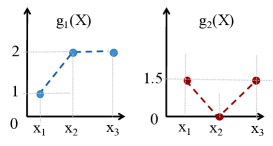
Consider two-armed bandit problem with reward functions $g_{1}$ and $g_{2}$ respectively, as shown in Figure 2. Suppose arm $1$ is pulled $10$ times, out of which we observe reward $1$ three times, and $2$ seven times, such that the empirical reward is

$$\hat{\mu}_{1} =\hat{p}_{1}+2(\hat{p}_{2}+\hat{p}_{3})=1.7$$ (3)

Using (3), we can estimate the distribution $(p_{1},p_{2},p_{3})$ of $X$ to be $\hat{p}_{1}=0.3$ and $\hat{p}_{2}+\hat{p}_{3}$ = 0.7. It is not possible to use this to estimate the reward of arm $2$ since we only know the sum $\hat{p}_{2}+\hat{p}_{3}$. However, we can find an upper bound on the empirical reward of arm $2$ as follows.

$$\hat{\mu}_{2} =1.5\hat{p}_{1}+0\hat{p}_{2}+1.5\hat{p}_{3}$$ (4)

$$\leq 1.5\hat{p}_{1}+\max(0,1.5)(\hat{p}_{2}+\hat{p}_{3})=1.5$$ (5)

Since the upper bound on arm $2$’s reward (which we refer to as its pseudo-reward) is less than arm $1$’s empirical reward, we consider arm $2$ as empirically non-competitive with respect to arm $1$ and do not pull it until it becomes empirically competitive again.

In Section 3 below we formalize the idea of competitive and non-competitive arms and propose a correlated upper confidence bound (C-UCB) algorithm. In Section 4 we give upper and lower bounds on the regret of the proposed algorithm, and show that the regret is similar to that of UCB with just $C+1$ arms instead of $K$ arms, where $C$ is the number of competitive arms.

3 C-UCB: The Proposed Correlated-UCB Algorithm

Our algorithm to choose an arm in each round in the correlated multi-armed bandit framework is a fundamental generalization of the upper confidence bound (UCB1) algorithm presented in (Auer et al., 2002). In round $t$, the UCB1 algorithm chooses the arm that maximizes the upper confidence index $I_{k}(t)$ which is defined as

$$I_{k}(t) =\hat{\mu}_{k}(t)+B\sqrt{\frac{2\log t}{n_{k}(t)}},$$ (6)

where $\hat{\mu}_{k}(t)$ is the empirical mean of the rewards received from arm $k$ until round $t$, and $n_{k}(t)$ is the number of times arm $k$ is pulled till round $t$. The second term causes the algorithm to explore arms that have been pulled only a few times (small $n_{k}(t)$). Recall that we assume all rewards to be bounded within an interval of size $B$. When the index $t$ is implied by context, we abbreviate $\hat{\mu}_{k}(t)$ and $I_{k}(t)$ to $\hat{\mu}_{k}$ and $I_{k}$ respectively in the rest of the paper. Also, we use the terms UCB1, UCB, and classic UCB interchangeably to refer to the UCB1 algorithm proposed in (Auer et al., 2002).

In correlated MAB framework, the rewards observed from one arm can help estimate the rewards from other arms. Our key idea is to use this information to reduce the amount of exploration required. We do so by evaluating the empirical pseudo-reward of every other arm $\ell$ with respect to an arm $k$, as we saw in 2. If this pseudo-reward is smaller than empirical reward of arm $k$, then arm $\ell$ is considered to be empirically non-competitive with respect to arm $k$, and we do not consider it as a candidate in the UCB1 algorithm.

The notions of pseudo-reward and empirical competitiveness of arms are defined in Section 3.1 and Section 3.2 below, and in Section 3.3 we describe how we modify the UCB1 algorithm. The pseudo-code of our algorithm is presented in Algorithm 1.

3.1 Pseudo-Reward of Arm $\ell$ with respect to Arm $k$

The pseudo-reward of arm $\ell$ with respect to arm $k$ is an artificial sample of arm $\ell$’s reward generated using the reward observed from arm $k$. It is defined as follows.

Definition 2 (Pseudo-Reward).

Suppose we pull arm $k$ and observe reward $r$. Then the pseudo-reward of arm $\ell$ with respect to arm $k$ is

$$s_{\ell,k}(r)\triangleq\max_{x:g_{k}(x)=r}g_{\ell}(x).$$ (7)

The pseudo-reward $s_{\ell,k}(r)$ gives the maximum possible reward that could have been obtained from arm $\ell$, given the reward observed from arm $k$. In 2, if we observe a reward of $r=2$ from arm $1$, $X$ could have been either $x_{2}$ or $x_{3}$. Then the pseudo-reward of arm $2$ is $s_{2,1}=1.5$ which is the maximum of $g_{2}(x_{2})$ and $g_{2}(x_{3})$. The pseudo-reward definition also applies to continuous $X$, and it can be directly extended to a latent random vector $\mathbf{X}=(X_{1},\dots X_{m})$ as well as explained in the supplementary material.

Definition 3 (Empirical and Expected Pseudo-Reward).

After $t$ rounds, arm $k$ is pulled $n_{k}(t)$ times. Using these $n_{k}(t)$ reward realizations, we can construct the empirical pseudo-reward $\hat{\phi}_{\ell,k}(t)$ for each arm $\ell$ with respect to arm $k$ as follows.

$$\hat{\phi}_{\ell,k}(t)\triangleq\frac{\sum_{\tau=1}^{t}\mathbbm{1}_{k_{\tau}=k}s_{\ell,k}(r_{t})}{n_{k}(t)},\qquad\ell\in\{1,\ldots,K\}\setminus\{k\}.$$ (8)

The expected pseudo-reward of arm $\ell$ with respect to arm $k$ is defined as

$$\phi_{\ell,k}\triangleq\mathbb{E}\left[{s_{\ell,k}(g_{k}(X))}\right].$$ (9)

 

1:  Input: Reward Functions $\{g_{1},g_{2}\ldots g_{K}\}$

2:  Initialize: $n_{k}=0,I_{k}=\infty$ for all $k\in\{1,2,\dots K\}$

3:  for  each round $t$ do

4:     Find $k^{\text{max}}=\arg\max_{k}n_{k}(t-1)$, the arm that has been pulled most times until round $t-1$

5:     Initialize the empirically competitive set $\mathcal{A}=\{1,2,\ldots,K\}\setminus\{k^{\text{max}}\}.$

6:     for $k\neq k^{\text{max}}$ do

7:        if $\hat{\mu}_{k^{\text{max}}}>\hat{\phi}_{k,k^{\text{max}}}$ then

8:           Remove arm $k$ from the empirically competitive set: $\mathcal{A}=\mathcal{A}\diagdown\{k\}$

9:        end if

10:     end for

11:     Apply UCB1 over arms in $\mathcal{A}\cup\{k^{\text{max}}\}$ by pulling arm $k_{t}=\arg\max_{k\in\mathcal{A}\cup\{k^{\text{max}}\}}I_{k}(t-1)$

12:     Receive reward $r_{t}$, and update $n_{k_{t}}=n_{k_{t}}+1$

13:     Update Empirical reward: $\hat{\mu}_{k_{t}}(t)=\frac{\hat{\mu}_{k_{t}}(t-1)(n_{k_{t}}(t)-1)+r_{t}}{n_{k_{t}}(t)}$

14:     Update the UCB Index: $I_{k_{t}}(t)=\hat{\mu}_{k_{t}}+B\sqrt{\frac{2\log t}{n_{k_{t}}}}$

15:     Compute pseudo-rewards for all arms $k\neq k_{t}$:    $s_{k,k_{t}}(r_{t})=\max_{x:g_{k_{t}}(x)=r_{t}}g_{k}(x).$

16:     Update empirical pseudo-rewards for all $k\neq k_{t}$: $\hat{\phi}_{k,k_{t}}(t)=\sum_{\tau:k_{\tau}=k_{t}}s_{k,k_{\tau}}(r_{\tau})/n_{k_{t}}$

17:  end for

 

Algorithm 1 C-UCB Correlated UCB Algorithm

Note that the empirical pseudo-reward $\hat{\phi}_{\ell,k}(t)$ is defined with respect to arm $k$ and it is only a function of the rewards observed by pulling $k$. It may be possible to get a more accurate estimate of arm $\ell$’s reward by combining the observations from all other arms. However, we consider this rough estimate, and it is sufficient to reduce $K$-armed bandit problem to a $C+1$ armed problem, as we show in Section 4.

3.2 Competitive and Non-competitive arms with respect to Arm $k$

Using the pseudo-reward estimates defined above, we can classify each arm $\ell\neq k$ as competitive or non-competitive with respect the arm $k$. To this end, we first define the notion of the pseudo-gap.

Definition 4 (Pseudo-Gap).

The pseudo-gap $\tilde{\Delta}_{\ell,k}$ of arm $\ell$ with respect to arm $k$ is defined as

$$\tilde{\Delta}_{\ell,k}\triangleq\mu_{k}-\phi_{\ell,k},$$ (10)

i.e., the difference between expected reward of arm $k$ and the expected pseudo-reward of arm $\ell$ with respect to arm $k$.

From the definition of pseudo-reward, it follows that the expected pseudo-reward $\phi_{\ell,k}$ is greater than or equal to the expected reward $\mu_{\ell}$ from arm $\ell$. Thus, a positive pseudo-gap $\tilde{\Delta}_{\ell,k}>0$ indicates that it is possible to classify arm $\ell$ as sub-optimal using only the rewards observed from arm $k$ (with high probability as the number of pulls for arm $k$ gets large); thus, arm $\ell$ needs not be explored. Such arms are called non-competitive, as we define below.

Definition 5 (Competitive and Non-Competitive arms).

An arm $\ell$ is said to be non-competitive if its pseudo-gap with respect to the optimal arm $k^{*}$ is positive, that is, $\tilde{\Delta}_{\ell,k^{*}}>0$. Similarly, an arm $\ell$ is said to be competitive if $\tilde{\Delta}_{\ell,k^{*}}<0$. The unique best arm $k^{*}$ has $\tilde{\Delta}_{k^{*},k^{*}}=0$ and is not counted in the set of competitive arms.

Since the distribution of $X$ is unknown, we can not find the pseudo-gap of each arm and thus have to resort to empirical estimates based on observed rewards. In our algorithm, we use a noisy notion of the competitiveness of an arm defined as follows. Note that since the optimal arm $k^{*}$ is also not known, empirical competitiveness of an arm $\ell$ is defined with respect to each of the other arms $k\neq\ell$.

Definition 6 (Empirically Competitive and Non-Competitive arms).

An arm $\ell$ is said to be “empirically non-competitive with respect to arm $k$ at round $t$" if its empirical pseudo-reward is less than the empirical reward of arm $k$, that is, $\hat{\mu}_{k}(t)-\hat{\phi}_{\ell,k}(t)>0$. Similarly, an arm $\ell\neq k$ is deemed empirically competitive with respect to arm $k$ at round $t$, if $\hat{\mu}_{k}(t)-\hat{\phi}_{\ell,k}(t)\leq 0$.

3.3 Modified UCB1 Algorithm to Eliminate Non-Competitive Arms

The central idea in our correlated UCB algorithm is that after pulling the optimal arm $k^{*}$ sufficiently large number of times, the non-competitive (and thus sub-optimal) arms can be classified as empirically non-competitive with increasing confidence, and thus need not be explored. As a result, the non-competitive arms will only be pulled only $\mathrm{O}(1)$ times. However, the competitive arms cannot be discerned as sub-optimal by just using the rewards observed from the optimal arm, and have to be explored $\Theta(\log T)$ times each. Thus, we are able to reduce a $K$-armed bandit to a $C+1$-armed bandit problem, where $C$ is the number of competitive arms.

Using this idea, our C-UCB algorithm proceeds as follows. After every round $t$, we maintain values for empirical reward, $\hat{\mu}_{k}(t)$, and the UCB1 index $I_{k}(t)$ for each arm $k$. These empirical estimates are based on the $n_{k}(t)$ samples of rewards that have been observed for $k$ till round $t$. In addition to this, we maintain empirical pseudo-reward of arm $\ell$ with respect to arm $k$, $\hat{\phi}_{\ell,k}(t)$, for all pairs of arms $(\ell,k)$. In each round $t$, the algorithm performs the following steps:

1. Select arm $k^{\textit{max}}=\arg\max_{k}n_{k}(t-1)$, that has been pulled the most until round $t-1$.

2. Identify the set $\mathcal{A}$ of arms that are empirically competitive with respect to arm $k^{\textit{max}}$.

3. Pull the arm $k_{t}\in\{\mathcal{A}\cup k^{\textit{max}}\}$ with the highest UCB1 index $I_{k}(t-1)$ (defined in (6)).

4. Update the empirical pseudo-rewards $s_{\ell,k_{t}}$ for all $\ell$, the empirical reward $\hat{\phi}_{\ell,k_{t}}(t)$, and the UCB1 indices of all arms based on the observed reward $r_{t}$.

In step $1$, we choose the arm that has been pulled the most number of times because we have the maximum number of reward samples from this arm. Thus, it is likely to most accurately identify the non-competitive arms. This property enables the proposed algorithm to achieve an $\mathrm{O}(1)$ regret contribution from non-competitive arms as we show in Section 4 below.

4 Regret Analysis and Bounds

We now characterize the performance of the C-UCB algorithm by analyzing the expected value of the cumulative regret (Definition 1). The expected regret can be expressed as

$$\mathbb{E}\left[{Reg(T)}\right] =\sum_{k=1}^{K}\mathbb{E}\left[{n_{k}(T)}\right]\Delta_{k},$$ (11)

where $\Delta_{k}=\mathbb{E}\left[{g_{k^{*}}(X)}\right]-\mathbb{E}\left[{g_{k}(X)}\right]=\mu_{k^{*}}-\mu_{k}$ is the sub-optimality gap of arm $k$ with respect to the optimal arm $k^{*}$, and $n_{k}(T)$ is the number of times arm $k$ is pulled in $T$ slots.

For the regret analysis, we assume without loss of generality that the reward functions $g_{k}(X)$ satisfy $0\leq g_{k}(X)\leq 1$ for all $k\in\{1,2,\dots K\}$. Note that the C-UCB algorithm does not require this condition on $g_{k}(X)$, and the regret analysis can also be generalized to any bounded reward functions.

4.1 Instance-Dependent Bounds

Most works on multi-armed bandits derive two types of bounds on expected regret: instance-dependent and worst case bounds, depending on whether or not the minimum sub-optimality gap $\Delta_{\text{min}}$ goes to $0$ with the total number of rounds $T$. Our instance-dependent bounds assume that the minimum gap $\Delta_{\text{min}}=\min_{k}\Delta_{k}$ remains strictly positive as the number of rounds $T\rightarrow\infty$, which is generally true in practice. Worst-case bounds are required when $\Delta_{\text{min}}$ can be arbitrarily small for large $T$. We derive both these bounds for the correlated-UCB algorithm. We use the standard Landau notation in the results, where all asymptotic statements are for large $T$. The proofs of all the results presented below are deferred to the supplement.

In order to bound $\mathbb{E}\left[{Reg(T)}\right]$ in (11), we can analyze the expected number of times sub-optimal arms are pulled, that is, $\mathbb{E}\left[{n_{k}(T)}\right]$, for all $k\neq k^{*}$. Theorem 1 and Theorem 2 below show that $\mathbb{E}\left[{n_{k}(T)}\right]$ scales as $O(1)$ and $O(\log T)$ for non-competitive and competitive arms respectively. Recall that a sub-optimal arm is said to be non-competitive if its pseudo-gap $\tilde{\Delta}_{k,k^{*}}>0$, and competitive otherwise.

Theorem 1 (Expected Pulls of a Non-competitive Arm).

If the pseudo-gap $\tilde{\Delta}_{k,k^{*}}\geq 2\sqrt{\frac{2K\log t_{0}}{t_{0}}}$, and the sub-optimality gap $\Delta_{\text{min}}\geq 4\sqrt{\frac{K\log t_{0}}{t_{0}}}$ for some constant $t_{0}>0$ then

$$\mathbb{E}\left[{n_{k}(T)}\right] \leq Kt_{0}+K(K-1)\sum_{t=Kt_{0}}^{T}3\left(\frac{t}{K}\right)^{-2}+\sum_{t=1}^{T}t^{-3},$$ (12)

$$=\mathrm{O}(1).$$ (13)

Theorem 2 (Expected Pulls of a Competitive Arm).

Expected number of times a competitive arm is pulled can be bounded as

$$\mathbb{E}\left[{n_{k}(T)}\right] \leq 8\frac{\log(T)}{\Delta_{k}^{2}}+\left(1+\frac{\pi^{2}}{3}\right)+\sum_{t=1}^{T}t\exp\left(-\frac{t\Delta_{\text{min}}^{2}}{2K}\right),$$ (14)

$$=\mathrm{O}(\log T)\quad\text{ if }\Delta_{\text{min}}=\min_{k}\Delta_{k}>0.$$ (15)

Substituting the bounds on $\mathbb{E}\left[{n_{k}(T)}\right]$ derived in Theorem 1 and Theorem 2 into (11), we get the following upper bound on expected regret.

Theorem 3 (Upper Bound on Expected Regret).

If the minimum sub-optimality gap $\Delta_{\text{min}}\geq 4\sqrt{\frac{K\log t_{0}}{t_{0}}}$, and the pseudo-gap of non-competitive arms $\tilde{\Delta}_{k,k^{*}}\geq 2\sqrt{\frac{2K\log t_{0}}{t_{0}}}$ for some constant $t_{0}>0$, then the expected cumulative regret of the C-UCB algorithm is

$$\mathbb{E}\left[{Reg(T)}\right] \leq\sum_{k\in\mathcal{C}}\Delta_{k}U^{(c)}_{k}(T)+\sum_{k^{\prime}\in\{1,\ldots,K\}\setminus\{\mathcal{C}\cup k^{*}\}}\Delta_{k^{\prime}}U^{(nc)}_{k^{\prime}}(T),$$ (16)

$$=C\cdot\mathrm{O}(\log T)+\mathrm{O}(1),$$ (17)

where $\mathcal{C}\subseteq\{1,\ldots,K\}\setminus\{k^{*}\}$ is set of competitive arms with cardinality $C$, $U^{(c)}_{k}(T)$ is the upper bound on $\mathbb{E}\left[{n_{k}(T)}\right]$ for competitive arms given in (14), and $U^{(nc)}_{k}(T)$ is the upper bound for non-competitive arms given in (12).

Remark 2.

If the set of competitive arms $\mathcal{C}$ is empty (i.e., the number of competitive arms $C=0$), then our algorithm will lead to (see (17)) an expected regret of $\mathrm{O}(1)$, instead of the typical $\mathrm{O}(\log T)$ regret scaling in classic multi-armed bandits. A simple case where $\mathcal{C}$ is empty is when the reward function $g_{k^{*}}(X)$ corresponding to the arm $k^{*}$ is invertible. This is because, for all sub-optimal arms $\ell\neq k^{*}$, the pseudo-gap $\tilde{\Delta}_{\ell,k^{*}}=\Delta_{\ell}>0$, resulting in those arms being non-competitive. The set $\mathcal{C}$ can be empty in more general cases where none of the arms are invertible. Then, our algorithm still achieves an expected regret of $\mathrm{O}(1)$.

Remark 3.

For the UCB1 algorithm (Auer et al., 2002), the first sum in (16) is taken over all arms. In this sense, our C-UCB algorithm is able to reduce a $K$-armed bandit problem to a $C+1$-armed bandit problem.

Next, we present a lower bound on the expected regret $\mathbb{E}\left[{Reg(T)}\right]$. Intuitively, if an arm $\ell$ is competitive, it can not be deemed sub-optimal by only pulling the optimal arm $k^{*}$ infinitely many times. This indicates that exploration is necessary for competitive arms. The proof of this bound closely follows that of the 2-armed classical bandit problem (Lai and Robbins, 1985); i.e., we construct a new bandit instance under which a previously sub-optimal arm becomes optimal without affecting reward distribution of any other arm.

Theorem 4 (Lower Bound on Expected Regret).

For any algorithm that achieves a sub-polynomial regret,

$$\lim_{T\rightarrow\infty}\inf\frac{\mathbb{E}\left[{Reg(T)}\right]}{\log(T)}\geq\begin{cases}\max_{k\in\mathcal{C}}\frac{\Delta_{k}}{D(f_{R_{k}}||f_{\tilde{R}_{k}})}\quad&\text{if }C>0,\\ 0\quad&\text{if }C=0.\end{cases}$$ (18)

Here $f_{R_{k}}$ is the reward distribution of arm $k$, which is linked with $f_{X}$ since $R_{k}=g_{k}(X)$. The term $f_{\tilde{R}_{k}}$ represents the reward distribution of arm $k$ in the new bandit instance where arm $k$ becomes optimal and distribution $f_{R_{k^{*}}}$ is unaffected. The divergence term represents "the amount of distortion needed in $f_{X}$ to make arm $k$ optimal", and hence captures the problem difficulty in the lower bound expression.

Remark 4.

From Theorem 3, we see that whenever $C>0$, our proposed algorithm achieves $\mathrm{O}(\log T)$ regret matching the lower bound given in Theorem 4 order-wise. Also, when $C=0$, our algorithm achieves $\mathrm{O}(1)$ regret. Thus, our algorithm achieves bounded regret whenever possible, i.e., when $C=0$.

4.2 Worst Case Bound on Expected Regret

Our instance-dependent bounds assumed that the minimum gap $\Delta_{\text{min}}\geq 4\sqrt{\frac{K\log t_{0}}{t_{0}}}$ for some $t_{0}>0$, with a similar assumption on the pseudo-gap. We now present an upper bound the on expected regret without this assumption, when $\Delta_{k}$ can scale with $T$ and become arbitrarily small as $T\rightarrow\infty$.

Theorem 5 (Worst Case Expected Regret).

In the worst case, the expected regret of the C-UCB algorithm is $\mathrm{O}(\sqrt{T\log(T)})$.

Note that this worst case regret bound is the same as that obtained for the UCB1 algorithm (Auer et al., 2002) when the arms are independent. This demonstrates that our algorithm can achieve the same order-wise worst case regret as classic UCB.

5 Simulation Results

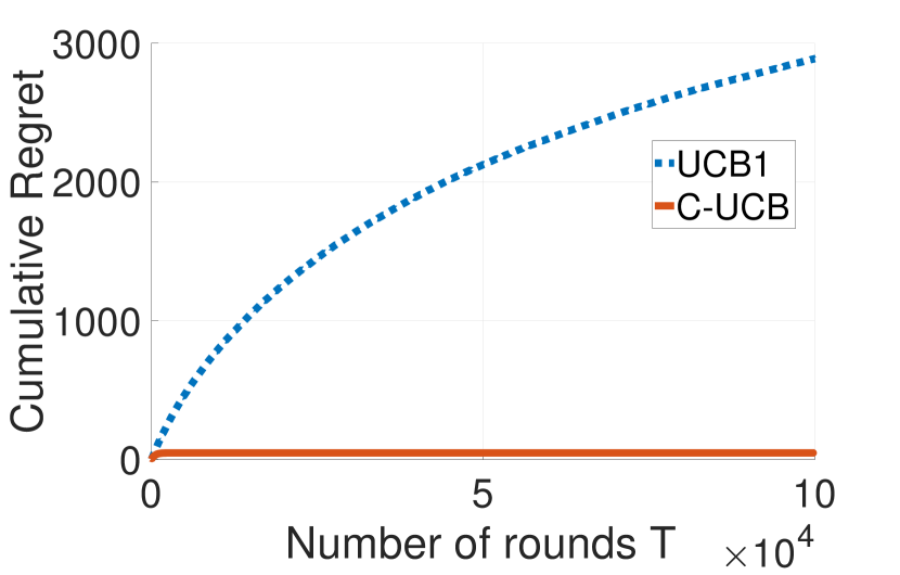
We now present simulation results for the case where $X$ is a discrete random variable (simulations for continuous $X$ and random vector $\mathbf{X}$ are shown in the supplement). We consider the reward functions $g_{1}(X),g_{2}(X)$ and $g_{3}(X)$ shown in Figure 3 for all simulation plots. However, the probability distribution ${P}_{X}=(p_{x_{1}},p_{x_{2}},\dots p_{x_{5}})$ of $X$ is different for each of the following cases given below. For each case, Figure 4 shows the cumulative regret versus the number of rounds. The cumulative regret is averaged over $500$ simulation runs, and for each run we use the same reward realizations for both the C-UCB and the vanilla UCB1 algorithms.

Figure 3: Reward Functions used for the simulation results presented in Figure 4.

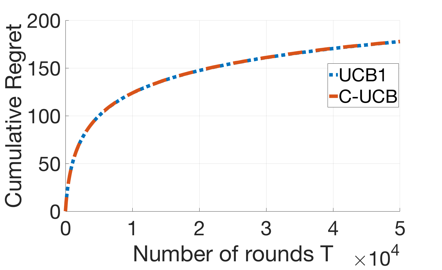
Case 1: No competitive arms. Here, we set ${P}_{X}=(0.1,0.2,0.25,0.25,0.2)$. For this probability distribution, arm $1$ is optimal, and arms $2$ and $3$ are non-competitive. Since both arm $2$ and arm $3$ are non-competitive, our result from Theorem 1 suggests that regret of C-UCB algorithm should not scale with the number of rounds $T$. This is supported by our simulation results as well. We see in Figure 4(a) that the proposed C-UCB algorithm achieves a constant regret and is significantly superior to the UCB1 algorithm as it is able to exploit the correlation of rewards between the arms.

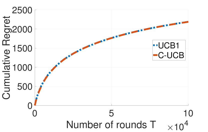
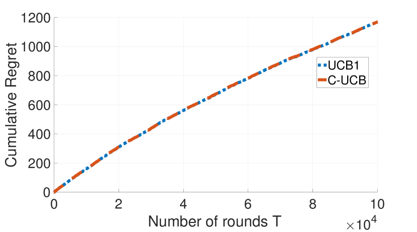
Case 2: One competitive arm. Let ${P}_{X}=(0.25,0.17,0.25,0.17,0.16)$ which results arm $3$ being optimal. Arm $1$ is non-competitive while arm $2$ is competitive. We expect from our results that number of pulls of arm $1$ should not scale with $T$, while the number of pulls for arm $2$ can scale with the $T$. This phenomenon can be seen in Figure 4(b). The regret of C-UCB algorithm is much smaller than the UCB1 algorithm as C-UCB algorithm is not exploring arm 1. However, the regret scales with the number of rounds $T$ as it is necessary to explore Arm 2.

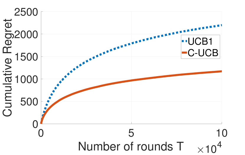
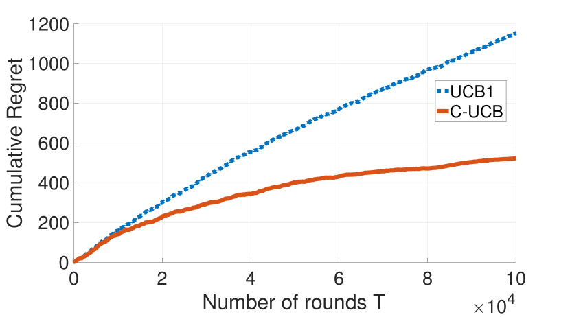
Case 3: Two competitive arms. In the last scenario, we set ${P}_{X}=(0.05,0.3,0.3,0.05,0.3)$. For this distribution, arm $3$ is optimal and arms $1$ and $2$ are both competitive. Since both arms are competitive, exploration is necessary for both arms. Therefore, as we see in Figure 4(c), the regret obtained under C-UCB and UCB1 are similar and scale with the number of rounds $T$.

(a) No competitive arms

(b) Only One Competitive arm

(c) Both Arms are Competitive

Figure 4: For the reward functions in Figure 3, the cumulative regret of C-UCB is smaller than vanilla-UCB1 in all the three cases above.

6 Concluding Remarks

This work studies a correlated multi-armed bandit (MAB) framework where the rewards obtained by pulling the $K$ different arms are functions of a common latent random variable $X$. We propose the C-UCB algorithm which achieves significant regret-reduction over the classic UCB. In fact, C-UCB is able to achieve a constant (instead of the standard logarithmic) regret in certain cases. A key idea behind the success of this algorithm is that correlation helps us use reward samples from one arm to generate pseudo-rewards from other arms, thus obviating the need to explore them. We believe that this idea is applicable more broadly to several other sequential decision-making problems. Ongoing work includes generalization of other multi-armed bandit algorithms such as Thompson sampling (Agrawal and Goyal, 2013), and understanding the scaling of regret with respect to the number of arms $K$. Instead of the deterministic reward functions $g_{i}(X)$, we also plan to consider random reward variables $Y_{i}$, such that the conditional distribution $p(Y_{i}|X)$ is known.

A Continuous $X$ and Random Vector $\mathbf{X}=(X_{1},X_{2},\ldots X_{m})$

Observe that our algorithm depends on the functions $g_{i}(X)$ through the evaluation of pseudo-rewards (see Definition 2). For discrete $X$, the set $\{x:g_{k}(x)=r\}$ is a discrete set with a finite number of elements. Hence, it is easy to evaluate $\max_{\{x:g_{k}(x)=r\}}g_{\ell}(x)$ for any arm $\ell\neq k$. For continuous $X$, if $\{x:g_{k}(x)=r\}$ is a finite union of continuous sets, and if $g_{\ell}(x)$ has finite stationary points, then it is possible to evaluate $g_{\ell}(x)$ for $x$ that lie at the boundary of continuous sets and at stationary points lying within these sets. Therefore, it is possible to compute $\max_{\{x:g_{k}(x)=r\}}g_{\ell}(x)$.

The algorithm and the regret analysis is also applicable to more general random sources, such as a latent random vector $\mathbf{X}=(X_{1},X_{2},\ldots X_{m})$. For example, if $X=(X_{1},X_{2})$ is a random variable, and $g_{1}(X)=X_{1}+0.1X_{2}$ and $g_{2}(X)=X_{2}+0.1X_{1}$. Then evaluating the pseudo-reward of arm 2 with respect to arm 1 on observing reward $r$ reduces to solving an optimization problem

$$\max_{z_{1},z_{2}} \quad z_{2}+0.1z_{1}$$

s.t $$\quad z_{1}+0.1z_{2}=r$$

$$\quad z_{1}\in\mathcal{W}_{1},z_{2}\in\mathcal{W}_{2},$$

where, $\mathcal{W}_{1},\mathcal{W}_{2}$ are support of $X_{1}$ and $X_{2}$ respectively.

As mentioned in Remark 1, this also captures the case of classical multi-armed bandit problem, if $\mathbf{X}=(X_{1},X_{2},\ldots X_{n})$, where $X_{i}$ are independent random variables and $g_{k}(X)=X_{k}$ for $k\in\{1,2,\ldots K\}$.

B Simulations for Continuous X and Random Vector $\mathbf{X}$

In this section we obtained cumulative regret by averaging over 100 simulation runs, for each run we use the same reward realizations for both the C-UCB and UCB1 ([5]) algorithm. We show these results for continuous X and random vector $\mathbf{X}$.

B.1 Continuous Random Variable

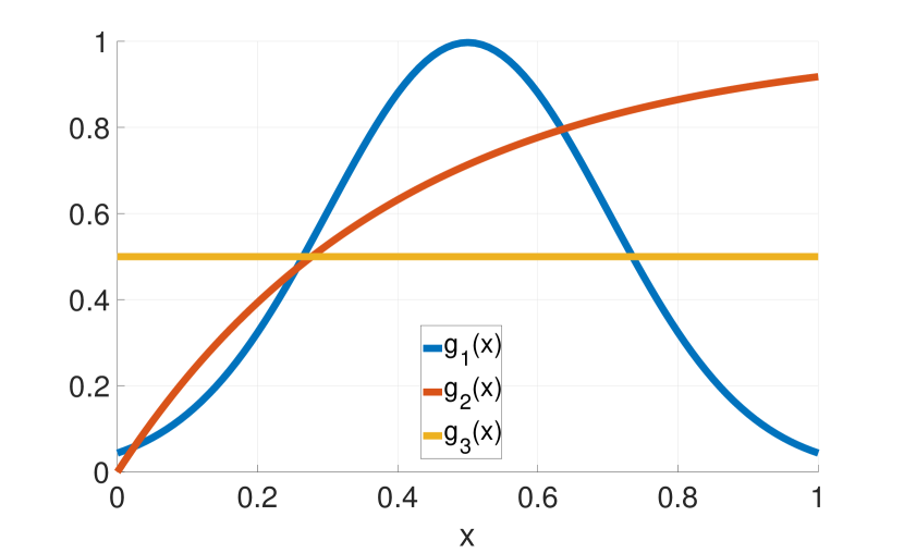
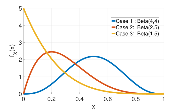
We consider the reward functions $g_{1}(X),g_{2}(X)$ and $g_{3}(X)$ as shown in Figure 6. Arm 1 corresponds to a Gaussian reward function $g_{1}(x)=\frac{1}{2\sqrt{2\pi\sigma^{2}}}\exp\left(-\frac{(x-\mu)^{2}}{2\sigma^{2}}\right)$, with $\mu=0.5$ and $\sigma=0.2$. Arm 2 corresponds to $g_{2}(x)=1-\exp(-5\lambda x)$, with $\lambda=0.5$. Arm 3 corresponds to a uniform reward function with $g_{3}(x)=0.5$. Depending on the distribution of random variable $X$, we can have different scenarios. For this simulation, we considered three cases with distribution of $X$ as $Beta(4,4),$ $Beta(2,5)$ and $Beta(1,5)$ respectively. Distribution of $X$ for these three cases is shown in Figure 6.

Figure 5: Reward Functions used for the simulation results presented in Figure 7.

Figure 6: Distribution of $X$ for the three cases of simulation results presented in Figure 7.

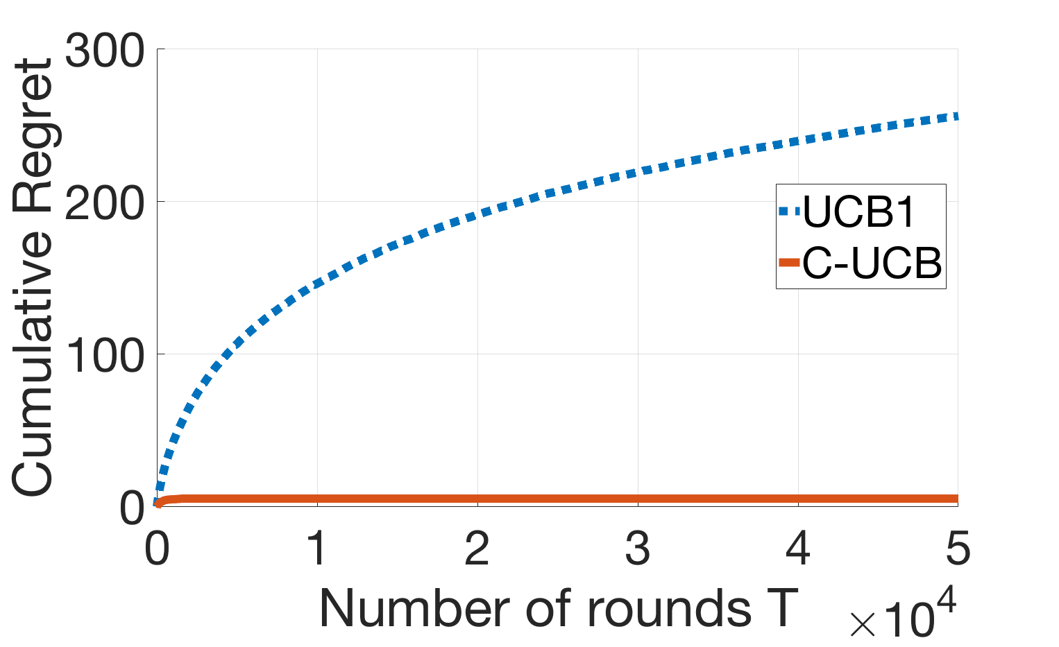
Case 1: $X\sim Beta(4,4)$. For this case arm 1 is the optimal arm, and arms 2 and 3 are non-competitive. As a result, the regret of C-UCB algorithm does not scale with the number of rounds. Observe that in Figure 7(a) the regret of C-UCB algorithm is very small; this is because the pseudo-gap of arms 2 and 3 with respect to arm 1 in this setting are large and hence sub-optimal arms are pulled very few times as they are easily identified as sub-optimal through pulls of Arm 1. This also demonstrates a case where sub-optimal arms are non-nompetitive even though the optimal arm is non-invertible.

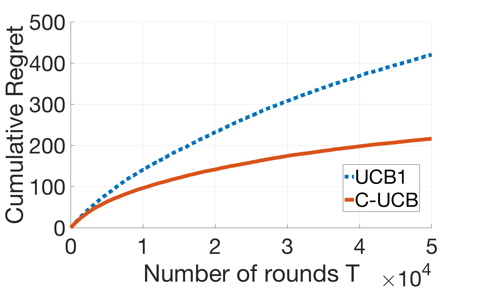
Case 2: $X\sim Beta(2,5)$. In this scenario arm 1 is the optimal arm, arm 2 is competitive and arm 3 is non-competitive. Due to this, C-UCB algorithm still explores arm 2. As evident in Figure 7(b), C-UCB clearly outperforms the UCB1 algorithm. This is because C-UCB algorithm explores only arm 2, while UCB1 explores both arm 1 and arm 2.

Case 3: $X\sim Beta(1,5)$. In this case, arm 3 is the optimal arm. Since pulls of arm 3 provide no information about reward from Arm 1 and Arm 2, both Arm 1 and Arm 2 are Competitive. Due to this C-UCB algorithm explores both the arms and has a performance very similar to the UCB1 algorithm as shown in Figure 7(c).

(a) Arm 1 is optimal, other two are non-competitive.

(b) Arm 1 is optimal, arm 2 is competitive and arm 3 is non-competitive.

(c) Arm 3 is optimal and arm 1, 2 are competitive.

Figure 7: Simulation results for continuous X.

B.2 Latent Random Vector $\mathbf{X}$

We now consider a case where we have a random vector $\mathbf{X}=(X_{1},X_{2})$. In our setting $X_{1},X_{2}$ have a support of $\{-1,0,1\}$. We consider two arms with $g_{1}(X)=X_{1}+X_{2}$ and $g_{2}(X)=X_{1}-X_{2}$. In this example $s_{2,1}(r)>g_{1}(r)$ only if the observed reward $r=2$, which corresponds to the case where the realization $(X_{1},X_{2})$ can be identified as $(1,1)$. Similarly $s_{1,2}(r)>g_{2}(r)$ only if the observed reward $r=2$, which corresponds to the realization $(1,-1)$. Depending on the distribution of $X$, suboptimal arm can be competitive or non-competitive.

Case 1: Suboptimal arm is Competitive. We consider a case where $\mathbb{P}_{\mathbf{X}}=\mathbb{P}_{X_{1}}\mathbb{P}_{X_{2}}$, with $\mathbb{P}_{X_{1}}=\{0.3,0.4,0.3\}$ and $\mathbb{P}_{X_{2}}=\{0.38,0.22,0.4\}$. In this scenario Arm 1 is optimal and sub-optimality gap of arm2 is $\Delta_{2}=0.04$. Since the probability mass on $(1,1)$ is small, Arm 2 is Competitive. Due to this, we see in Figure 8(a) that regret of the C-UCB algorithm scales with number of rounds $T$ and has a performance very similar to the UCB1 algorithm.

Case 2: Suboptimal arm is Non-Competitve We consider the distribution $\mathbb{P}_{\mathbf{X}}$ with $\mathbb{P}_{\mathbf{X}}(1,-1)=0.48$, $\mathbb{P}_{\mathbf{X}}(1,1)=0.5$ and $\mathbb{P}_{\mathbf{X}}(x_{1},x_{2})=0.0028$ for all other $x_{1},x_{2}$. In this scenario, arm $1$ is optimal and arm $2$ is sub-optimal with suboptimality gap $\Delta_{2}=0.04$. Since probability mass at $(1,1)$ is high, it is possible to infer sub-optimality of arm 2 using reward samples of arm 1. We see this effect in Figure 8(b).

(a) Sub-optimal arm is competitive.

(b) Sub-optimal arm is non-competitive.

Figure 8: Simulation results for latent vector $\mathbf{X}$.

C Standard Results from Previous Works

Fact 1 (Hoeffding’s inequality).

Let $Z_{1},Z_{2}\ldots Z_{n}$ be i.i.d random variables bounded between $[a,b]:a\leq Z_{i}\leq b$, then for any $\delta>0$, we have

$$\Pr\left(\left|\frac{\sum_{i=1}^{n}Z_{i}}{n}-\mathbb{E}\left[{Z_{i}}\right]\right|\geq\delta\right)\leq\exp\left(\frac{-2n\delta^{2}}{(b-a)^{2}}\right).$$

Lemma 1 (Standard result used in bandit literature).

If $\hat{\mu}_{k,n_{k}(t)}$ denotes the empirical mean of arm $k$ by pulling arm $k$ $n_{k}(t)$ times through any algorithm and $\mu_{k}$ denotes the mean reward of arm $k$, then we have

$$\Pr\left(\hat{\mu}_{k,n_{k}(t)}-\mu_{k}\geq\epsilon,\tau_{2}\geq n_{k}(t)\geq\tau_{1}\right)\leq\sum_{s=\tau_{1}}^{\tau_{2}}\exp\left(-2s\epsilon^{2}\right).$$

Proof.

Let $Z_{1},Z_{2},...Z_{t}$ be the reward samples of arm $k$ drawn separately. If the algorithm chooses to play arm $k$ for $m^{th}$ time, then it observes reward $Z_{m}$. Then the probability of observing the event $\hat{\mu}_{k,n_{k}(t)}-\mu_{k}\geq\epsilon,\tau_{2}\geq n_{k}(t)\geq\tau_{1}$ can be upper bounded as follows,

$$\Pr\left(\hat{\mu}_{k,n_{k}(t)}-\mu_{k}\geq\epsilon,\tau_{2}\geq n_{k}(t)\geq\tau_{1}\right) =\Pr\left(\left(\frac{\sum_{i=1}^{n_{k}(t)}Z_{i}}{n_{k}(t)}-\mu_{k}\geq\epsilon\right),\tau_{2}\geq n_{k}(t)\geq\tau_{1}\right)$$ (19)

$$\leq\Pr\left(\left(\bigcup_{m=\tau_{1}}^{\tau_{2}}\frac{\sum_{i=1}^{m}Z_{i}}{m}-\mu_{k}\geq\epsilon\right),\tau_{2}\geq n_{k}(t)\geq\tau_{1}\right)$$ (20)

$$\leq\Pr\left(\bigcup_{m=\tau_{1}}^{\tau_{2}}\frac{\sum_{i=1}^{m}Z_{i}}{m}-\mu_{k}\geq\epsilon\right)$$ (21)

$$\leq\sum_{s=\tau_{1}}^{\tau_{2}}\exp\left(-2s\epsilon^{2}\right).$$ (22)

∎

Lemma 2 (From Proof of Theorem 1 in [5]).

Let $I_{k}(t)$ denote the UCB index of arm $k$ at round $t$, and $\mu_{k}=\mathbb{E}\left[{g_{k}(X)}\right]$ denote the mean reward of that arm. Then, we have

$$\Pr(\mu_{k}>I_{k}(t))\leq t^{-3}.$$

Observe that this bound does not depend on the number $n_{k}(t)$ of times arm $k$ is pulled. UCB index is defined in equation (6) of the main paper.

Proof.

This proof follows directly from [5]. We present the proof here for completeness as we use this frequently in the paper.

$$\Pr(\mu_{k}>I_{k}(t)) =\Pr\left(\mu_{k}>\hat{\mu}_{k,n_{k}(t)}+\sqrt{\frac{2\log t}{n_{k}(t)}}\right)$$ (23)

$$\leq\sum_{m=1}^{t}\Pr\left(\mu_{k}>\hat{\mu}_{k,m}+\sqrt{\frac{2\log t}{m}}\right)$$ (24)

$$=\sum_{m=1}^{t}\Pr\left(\hat{\mu}_{k,m}-\mu_{k}<-\sqrt{\frac{2\log t}{m}}\right)$$ (25)

$$\leq\sum_{m=1}^{t}\exp\left(-2m\frac{2\log t}{m}\right)$$ (26)

$$=\sum_{m=1}^{t}t^{-4}$$ (27)

$$=t^{-3}.$$ (28)

where (24) follows from the union bound and is a standard trick (Lemma 1) to deal with random variable $n_{k}(t)$. We use this trick repeatedly in the proofs. We have (26) from the Hoeffding’s inequality. ∎

Lemma 3.

Let $\mathbb{E}\left[{\mathbbm{1}_{I_{k}>I_{k^{*}}}}\right]$ be the expected number of times $I_{k}(t)>I_{k^{*}}(t)$ in $T$ rounds. Then, we have

$$\mathbb{E}\left[{\mathbbm{1}_{I_{k}>I_{k^{*}}}}\right]=\sum_{t=1}^{T}Pr(I_{k}>I_{k^{*}})\leq\frac{8\log(T)}{\Delta_{k}^{2}}+\left(1+\frac{\pi^{2}}{3}\right).$$

The proof follows the analysis in Theorem 1 of [5]. The analysis of $Pr(I_{k}>I_{k^{*}})$ is done by conditioning on the event that Arm $k$ has been pulled $\frac{8\log(T)}{\Delta_{k}^{2}}$. Conditioned on this event, $Pr(I_{k}(t)>I_{k^{*}}(t)|n_{k}(t))\leq t^{-2}$.

Lemma 4 (Theorem 2 [15]).

Consider a two armed bandit problem with reward distributions $\Theta=\{f_{R_{1}}(r),f_{R_{2}}(r)\}$, where the reward distribution of the optimal arm is $f_{R_{1}}(r)$ and for the sub-optimal arm is $f_{R_{2}}(r)$, and $\mathbb{E}\left[{f_{R_{1}}(r)}\right]>\mathbb{E}\left[{f_{R_{2}}(r)}\right]$; i.e., arm 1 is optimal. If it is possible to create an alternate problem with distributions $\Theta^{\prime}=\{f_{R_{1}}(r),\tilde{f}_{R_{2}}(r)\}$ such that $\mathbb{E}\left[{\tilde{f}_{R_{2}}(r)}\right]>\mathbb{E}\left[{f_{R_{1}}(r)}\right]$ and $0<D(f_{R_{2}}(r)||\tilde{f}_{R_{2}}(r))<\infty$ (equivalent to assumption 1.6 in [15]), then for any policy that achieves sub-polynomial regret, we have

$$\liminf\limits_{T\rightarrow\infty}\frac{\mathbb{E}\left[{n_{2}(T)}\right]}{\log T}\geq\frac{1}{D(f_{R_{2}}(r)||\tilde{f}_{R_{2}}(r))}.$$

Proof.

Proof of this is derived from the analysis done in [16]. We show the analysis here for completeness. A bandit instance $v$ is defined by the reward distribution of arm 1 and arm 2. Since policy $\pi$ achieves sub-polynomial regret, for any instance $v$, $\mathbb{E}_{v,\pi}\left[(Reg(T))\right]=\mathrm{O}(T^{p})$ as $T\rightarrow\infty$, for all $p>0$.

Consider the bandit instances $\Theta=\{f_{R_{1}}(r),f_{R_{2}}(r)\}$, $\Theta^{\prime}=\{f_{R_{1}}(r),\tilde{f}_{R_{2}}(r)\}$, where $\mathbb{E}\left[{f_{R_{2}}(r)}\right]<\mathbb{E}\left[{f_{R_{1}}(r)}\right]<\mathbb{E}\left[{\tilde{f}_{R_{2}}(r)}\right]$. The bandit instance $\Theta^{\prime}$ is constructed by changing the reward distribution of arm 2 in the original instance, in such a way that arm 2 becomes optimal in instance $\Theta^{\prime}$ without changing the reward distribution of arm 1 from the original instance.

From divergence decomposition lemma (derived in [16]), it follows that

$$D(\mathbb{P}_{\Theta,\Pi}||\mathbb{P}_{\Theta^{\prime},\Pi})=\mathbb{E}_{\Theta,\pi}\left[n_{2}(T)\right]D(f_{R_{2}}(r)||\tilde{f}_{R_{2}}(r)).$$

The high probability Pinsker’s inequality (Lemma 2.6 from [27], originally in [7]) gives that for any event $A$,

$$\mathbb{P}_{\Theta,\pi}(A)+\mathbb{P}_{\Theta^{\prime},\pi}(A^{c})\geq\frac{1}{2}\exp\left(-D(\mathbb{P}_{\Theta,\pi}||\mathbb{P}_{\Theta^{\prime},\pi})\right),$$

or equivalently,

$$D(\mathbb{P}_{\Theta,\pi}||\mathbb{P}_{\Theta^{\prime},\pi})\geq\log\frac{1}{2(\mathbb{P}_{\Theta,\pi}(A)+\mathbb{P}_{\Theta^{\prime},\pi}(A^{c}))}.$$

If arm 2 is suboptimal in a 2-armed bandit problem, then $\mathbb{E}\left[{Reg(T)}\right]=\Delta_{2}\mathbb{E}\left[{n_{2}(T)}\right].$ Expected regret in $\Theta$ is

$$\mathbb{E}_{\Theta,\pi}\left[Reg(T)\right]\geq\frac{T\Delta_{2}}{2}\mathbb{P}_{\Theta,\pi}\left(n_{2}(T)\geq\frac{T}{2}\right),$$

Similarly regret in bandit instance $\Theta^{\prime}$ is

$$\mathbb{E}_{\Theta^{\prime},\pi}\left[Reg(T)\right]\geq\frac{T\delta}{2}\mathbb{P}_{\Theta^{\prime},\pi}\left(n_{2}(T)<\frac{T}{2}\right),$$

since suboptimality gap of arm $1$ in $\Theta^{\prime}$ is $\delta$. Define $\kappa(\Delta_{2},\delta)=\frac{\min(\Delta_{2},\delta)}{2}$. Then we have,

$$\mathbb{P}_{\Theta,\pi}\left(n_{2}(T)\geq\frac{T}{2}\right)+\mathbb{P}_{\Theta^{\prime},\pi}\left(n_{2}(T)<\frac{T}{2}\right)\leq\frac{\mathbb{E}_{\Theta,\pi}\left[Reg(T)\right]+\mathbb{E}_{\Theta^{\prime},\pi}\left[Reg(T)\right]}{\kappa(\Delta_{2},\delta)T}.$$

On applying the high probability Pinsker’s inequality and divergence decomposition lemma stated earlier, we get

$$D(f_{R_{2}}(r)||\tilde{f}_{R_{2}}(r))\mathbb{E}_{\Theta,\pi}\left[n_{2}(T)\right] \geq\log\left(\frac{\kappa(\Delta_{2},\delta)T}{2(\mathbb{E}_{\Theta,\pi}\left[Reg(T)\right]+\mathbb{E}_{\Theta^{\prime},\pi}\left[Reg(T)\right])}\right)$$ (29)

$$=\log\left(\frac{\kappa(\Delta_{2},\delta)}{2}\right)+\log(T)$$

$$\qquad-\log(\mathbb{E}_{\Theta,\pi}\left[Reg(T)\right]+\mathbb{E}_{\Theta^{\prime},\pi}\left[Reg(T)\right]).$$ (30)

Since policy $\pi$ achieves sub-polynomial regret for any bandit instance, $\mathbb{E}_{\Theta,\pi}\left[Reg(T)\right]+\mathbb{E}_{\Theta^{\prime},\pi}\left[Reg(T)\right]\leq\gamma T^{p}$ for all $T$ and any $p>0$, hence,

$$\liminf\limits_{T\rightarrow\infty}D(f_{R_{2}}(r)||\tilde{f}_{R_{2}}(r))\frac{\mathbb{E}_{\Theta,\pi}\left[n_{2}(T)\right]}{\log T} \geq 1-\limsup\limits_{T\rightarrow\infty}\frac{\mathbb{E}_{\Theta,\pi}\left[Reg(T)\right]+\mathbb{E}_{\Theta^{\prime},\pi}\left[Reg(T)\right]}{\log T}+$$

$$\quad\liminf\limits_{T\rightarrow\infty}\frac{\log\left(\frac{\kappa(\Delta_{2},\delta)}{2}\right)}{\log T}$$ (31)

$$=1.$$ (32)

Hence, $\liminf\limits_{T\rightarrow\infty}\frac{\mathbb{E}_{\Theta,\pi}\left[n_{2}(T)\right]}{\log T}\geq\frac{1}{D(f_{R_{2}}(r)||\tilde{f}_{R_{2}}(r))}.$

∎

D Lemmas Required to Prove Theorems 1, 2, 3, and 5

Lemma 5.

Define $E_{1}(t)$ to be the event that arm $k^{*}$ is empirically non-competitive in round $t+1$, then,

$$\Pr(E_{1}(t))\leq t\exp\left(\frac{-t\Delta_{\text{min}}^{2}}{2K}\right),$$

where $\Delta_{\text{min}}=\min_{k}\Delta_{k}$, the gap between the best and second-best arms.

Proof.

We analyze the probability that arm $k^{*}$ is empirically non competitive by conditioning on the event that arm $k^{*}$ is not pulled for maximum number of times till round $t$. Analyzing this expression gives us,

$$\Pr(E_{1}(t)) =\Pr(E_{1}(t),n_{k^{*}}(t)\neq\max_{k}n_{k}(t))$$ (33)

$$=\sum_{k\neq k^{*}}Pr(E_{1}(t),n_{k}(t)=\max_{k^{\prime}}n_{k^{\prime}}(t))$$ (34)

$$\leq\max_{k}\Pr(E_{1}(t),n_{k}(t)=\max_{k^{\prime}}n_{k^{\prime}}(t))$$ (35)

$$=\max_{k}\Pr(\hat{\mu}_{k}>\hat{\phi}_{k^{*},k},n_{k}(t)=\max_{k^{\prime}}n_{k^{\prime}}(t))$$ (36)

$$\leq\max_{k}\Pr\left(\hat{\mu}_{k}>\hat{\phi}_{k^{*},k},n_{k}(t)\geq\frac{t}{K}\right)$$ (37)

$$=\max_{k}\Pr\left(\frac{\sum_{\tau=1}^{t}\mathbbm{1}_{\{k_{\tau}=k\}}r_{\tau}}{n_{k}(t)}>\frac{\sum_{\tau=1}^{t}\mathbbm{1}_{\{k_{\tau}=k\}}s_{k^{*},k}(r_{\tau})}{n_{k}(t)},n_{k}(t)\geq\frac{t}{K}\right)$$ (38)

$$=\max_{k}\Pr\left(\frac{\sum_{\tau=1}^{t}\mathbbm{1}_{\{k_{\tau}=k\}}\left(r_{\tau}-s_{k^{*},k}(r_{\tau})\right)}{n_{k}(t)}>0,n_{k}(t)\geq\frac{t}{K}\right)$$ (39)

$$=\max_{k}\Pr\left(\frac{\sum_{\tau=1}^{t}\mathbbm{1}_{\{k_{\tau}=k\}}\left(r_{\tau}-s_{k^{*},k}(r_{\tau})\right)}{n_{k}(t)}-(\mu_{k}-\phi_{k^{*},k})>\phi_{k^{*},k}-\mu_{k},n_{k}(t)\geq\frac{t}{K}\right)$$ (40)

$$\leq\max_{k}\Pr\left(\frac{\sum_{\tau=1}^{t}\mathbbm{1}_{\{k_{\tau}=k\}}\left(r_{\tau}-s_{k^{*},k}(r_{\tau})\right)}{n_{k}(t)}-(\mu_{k}-\phi_{k^{*},k})>\Delta_{k},n_{k}(t)\geq\frac{t}{K}\right)$$ (41)

$$\leq\max_{k}t\exp\left(\frac{-t\Delta_{k}^{2}}{2K}\right)$$ (42)

$$=t\exp\left(\frac{-t\Delta_{\text{min}}^{2}}{2K}\right),$$ (43)

Here (36) follows from the fact that in order for arm $k^{*}$ to be empirically non-competitive, empirical mean of arm $k$ should be more than empirical pseudo-reward of arm $k^{*}$ with respect to arm $k$. Inequality (37) follows since $n_{k}(t)$ being more than $\frac{t}{K}$ is a necessary condition for $n_{k}(t)=\max_{k^{\prime}}n_{k^{\prime}}(t)$ to occur. We have (41) as $s_{k^{*},k}$ is more than $\mu_{k^{*}}$. We have (42) from the Hoeffding’s inequality, as we note that rewards $\{r_{\tau}-s_{k^{*},k}(r_{\tau}):\tau=1,\ldots,t,~{}k_{\tau}=k\}$ form a collection of i.i.d. random variables each of which is bounded between $[-1,1]$ with mean $(\mu_{k}-\phi_{k^{*},k})$. The term $t$ before the exponent in (42) arises as the random variable $n_{k}(t)$ can take values from $t/K$ to $t$ (Lemma 1). ∎

Lemma 6.

If $\Delta_{\text{min}}\geq 4\sqrt{\frac{K\log t_{0}}{t_{0}}}$ for some constant $t_{0}>0$, then,

$$\Pr(k_{t+1}=k,n_{k}(t)\geq s)\leq 3t^{-3}\quad\text{for }s>\frac{t}{2K},\forall t>t_{0}.$$

Proof.

By noting that $k_{t+1}=k$ corresponds to arm $k$ having the highest index among the set of arms that are not empirically non-competitive (denoted by $\mathcal{A}$), we have,

$$\Pr(k_{t+1}=k,n_{k}(t)\geq s) =\Pr(I_{k}(t)=\arg\max_{k^{\prime}\in\mathcal{A}}I_{k^{\prime}}(t),n_{k}(t)\geq s)$$ (44)

$$\leq\Pr(E_{1}(t)\cup\left(E_{1}^{c}(t),I_{k}(t)>I_{k^{*}}(t)\right),n_{k}(t)\geq s)$$ (45)

$$\leq\Pr(E_{1}(t),n_{k}(t)\geq s)+\Pr(E_{1}^{c}(t),I_{k}(t)>I_{k^{*}}(t),n_{k}(t)\geq s)$$ (46)

$$\leq t\exp\left(\frac{-t\Delta_{\text{min}}^{2}}{2K}\right)+\Pr\left(I_{k}(t)>I_{k^{*}}(t),n_{k}(t)\geq s\right).$$ (47)

Here $E_{1}(t)$ is the event described in Lemma 5. If arm $k^{*}$ is not empirically non-competitive at round $t$, then arm $k$ can only be pulled in round $t+1$ if $I_{k}(t)>I_{k^{*}}(t)$, due to which we have (45). Inequalities (46) and (47) follow from union bound and Lemma 5 respectively.

We now bound the second term in (47).

$$\Pr(I_{k}(t)>I_{k^{*}}(t),n_{k}(t)\geq s)$$

$$=\Pr\left(I_{k}(t)>I_{k^{*}}(t),n_{k}(t)\geq s,\mu_{k^{*}}\leq I_{k^{*}}(t)\right)+$$

$$\quad\Pr\left(I_{k}(t)>I_{k^{*}}(t),n_{k}(t)\geq s|\mu_{k^{*}}>I_{k^{*}}(t)\right)\times\Pr\left(\mu_{k^{*}}>I_{k^{*}}(t)\right)$$ (48)

$$\leq\Pr\left(I_{k}(t)>I_{k^{*}}(t),n_{k}(t)\geq s,\mu_{k^{*}}\leq I_{k^{*}}(t)\right)+\Pr\left(\mu_{k^{*}}>I_{k^{*}}(t)\right)$$ (49)

$$\leq\Pr\left(I_{k}(t)>I_{k^{*}}(t),n_{k}(t)\geq s,\mu_{k^{*}}\leq I_{k^{*}}(t)\right)+t^{-3}$$ (50)

$$=\Pr\left(I_{k}(t)>\mu_{k^{*}},n_{k}(t)\geq s\right)+t^{-4}$$ (51)

$$=\Pr\left(\hat{\mu}_{k}(t)+\sqrt{\frac{2\log t}{n_{k}(t)}}>\mu_{k^{*}},n_{k}(t)\geq s\right)+t^{-3}$$ (52)

$$=\Pr\left(\hat{\mu}_{k}(t)-\mu_{k}>\mu_{k^{*}}-\mu_{k}-\sqrt{\frac{2\log t}{n_{k}(t)}},n_{k}(t)\geq s\right)+t^{-3}$$ (53)

$$=\Pr\left(\frac{\sum_{\tau=1}^{t}\mathbbm{1}_{\{k_{\tau}=k\}}r_{\tau}}{n_{k}(t)}-\mu_{k}>\Delta_{k}-\sqrt{\frac{2\log t}{n_{k}(t)}},n_{k}(t)\geq s\right)+t^{-3}$$ (54)

$$\leq t\exp\left(-2s\left(\Delta_{k}-\sqrt{\frac{2\log t}{s}}\right)^{2}\right)+t^{-3}$$ (55)

$$\leq t^{-3}\exp\left(-2s\left(\Delta_{k}^{2}-2\Delta_{k}\sqrt{\frac{2\log t}{s}}\right)\right)+t^{-3}$$ (56)

$$\leq 2t^{-3}\quad\text{ for all }t>t_{0}.$$ (57)

We have (48) holds because of the fact that $P(A)=P(A|B)P(B)+P(A|B^{c})P(B^{c})$, Inequality (50) follows from Lemma 2. From the definition of $I_{k}(t)$ we have (52). Inequality (55) follows from Hoeffding’s inequality and the term $t$ before the exponent in (42) arises as the random variable $n_{k}(t)$ can take values from $s$ to $t$ (Lemma 1). Inequality (57) follows from the fact that $s>\frac{t}{2K}$ and $\Delta_{k}\geq 4\sqrt{\frac{K\log t_{0}}{t_{0}}}$ for some constant $t_{0}>0.$

Plugging this in the expression of $\Pr(k_{t}=k\mid n_{k}(t)\geq s)$ (47) gives us,

$$\Pr(k_{t+1}=k\mid n_{k}(t)\geq s) \leq t\exp\left(\frac{-t\Delta_{\text{min}}^{2}}{2K}\right)+\Pr(I_{k}(t)>I_{k^{*}}(t)|n_{k}(t)\geq s)$$ (58)

$$\leq t\exp\left(\frac{-t\Delta_{\text{min}}^{2}}{2K}\right)+2t^{-3}$$ (59)

$$\leq 3t^{-3}.$$ (60)

Here, (60) follows from the fact that $\Delta_{\text{min}}\geq 2\sqrt{\frac{2K\log t_{0}}{t_{0}}}$ for some constant $t_{0}>0$. ∎

Lemma 7.

If for a suboptimal arm $k\neq k^{*}$, $\tilde{\Delta}_{k,k^{*}}>0$, then,

$$\Pr(k_{t+1}=k,n_{k^{*}}(t)=\max_{k}n_{k})\leq t\exp\left(\frac{-t\tilde{\Delta}_{k,k^{*}}^{2}}{2K}\right).$$

Moreover, if $\tilde{\Delta}_{k,k^{*}}\geq 2\sqrt{\frac{2K\log t_{0}}{t_{0}}}$ for some constant $t_{0}>0$. Then,

$$\Pr(k_{t+1}=k,n_{k^{*}}(t)=\max_{k}n_{k})\leq t^{-3}\quad\forall t>t_{0}.$$

Proof.

We now bound this probability as,

$$\Pr(k_{t+1}=k,n_{k^{*}}=\max_{k}n_{k})$$

$$=\Pr\left(\hat{\mu}_{k^{*}}(t)<\hat{\phi}_{k,k^{*}}(t),I_{k}(t)=\max_{k^{\prime}}I_{k^{\prime}}(t),n_{k^{*}}(t)=\max_{k}n_{k}(t)\right)$$ (61)

$$\leq\Pr\left(\hat{\mu}_{k^{*}}(t)<\hat{\phi}_{k,k^{*}}(t),n_{k^{*}}(t)=\max_{k}n_{k}(t)\right)$$ (62)

$$\leq\Pr\left(\hat{\mu}_{k^{*}}(t)<\hat{\phi}_{k,k^{*}}(t),n_{k^{*}}(t)\geq\frac{t}{K}\right)$$ (63)

$$\leq\Pr\left(\frac{\sum_{\tau=1}^{t}\mathbbm{1}_{\{k_{\tau}=k^{*}\}}r_{\tau}}{n_{k^{*}}(t)}<\frac{\sum_{\tau=1}^{t}\mathbbm{1}_{\{k_{\tau}=k^{*}\}}s_{k,k^{*}}(r_{\tau})}{n_{k^{*}(t)}},n_{k^{*}}(t)\geq\frac{t}{K}\right)$$ (64)

$$=\Pr\left(\frac{\sum_{\tau=1}^{t}\mathbbm{1}_{\{k_{\tau}=k^{*}\}}(r_{\tau}-s_{k,k^{*}})}{n_{k^{*}}(t)}-(\mu_{k^{*}}-\phi_{k,k^{*}})<-\tilde{\Delta}_{k,k^{*}},n_{k^{*}}\geq\frac{t}{K}\right)$$ (65)

$$\leq t\exp\left(\frac{-t\tilde{\Delta}_{k,k^{*}}^{2}}{2K}\right)$$ (66)

$$\leq t^{-3}\quad\forall t>t_{0}.$$ (67)

Here, (65) follows from the Hoeffding’s inequality as we note that rewards $\{r_{\tau}-s_{k,k^{*}}(r_{\tau}):\tau=1,\ldots,t,~{}k_{\tau}=k\}$ form a collection of i.i.d. random variables each of which is bounded between $[-1,1]$ with mean $(\mu_{k}-\phi_{k,k^{*}})$. The term $t$ before the exponent in (65) arises as the random variable $n_{k}(t)$ can take values from $t/K$ to $t$ (Lemma 1). Step (67) follows from the fact that $\tilde{\Delta}_{k,k^{*}}\geq 2\sqrt{\frac{2K\log t_{0}}{t_{0}}}$ for some constant $t_{0}>0$. ∎

Lemma 8.

If $\Delta_{\text{min}}\geq 4\sqrt{\frac{K\log t_{0}}{t_{0}}}$ for some constant $t_{0}>0$, then,

$$\Pr\left(n_{k}(t)>\frac{t}{K}\right)\leq 3K\left(\frac{t}{K}\right)^{-2}\quad\forall t>Kt_{0}.$$

Proof.

We expand $\Pr\left(n_{k}(t)>\frac{t}{K}\right)$ as,

$$\Pr\left(n_{k}(t)\geq\frac{t}{K}\right) =\Pr\left(n_{k}(t)\geq\frac{t}{K}\mid n_{k}(t-1)\geq\frac{t}{K}\right)\Pr\left(n_{k}(t-1)\geq\frac{t}{K}\right)+$$

$$\quad\Pr\left(k_{t}=k,n_{k}(t-1)=\frac{t}{K}-1\right)$$ (68)

$$\leq\Pr\left(n_{k}(t-1)\geq\frac{t}{K}\right)+\Pr\left(k_{t}=k,n_{k}(t-1)=\frac{t}{K}-1\right)$$ (69)

$$\leq\Pr\left(n_{k}(t-1)\geq\frac{t}{K}\right)+3(t-1)^{-3}\quad\forall(t-1)>t_{0}.$$ (70)

Here, (70) follows from Lemma 6.

This gives us

$$\Pr\left(n_{k}(t)\geq\frac{t}{K}\right)-\Pr\left(n_{k}(t-1)\geq\frac{t}{K}\right)\leq 3(t-1)^{-3},\quad\forall(t-1)>t_{0}.$$

Now consider the summation

$$\sum_{\tau=\frac{t}{K}}^{t}\Pr\left(n_{k}(\tau)\geq\frac{t}{K}\right)-\Pr\left(n_{k}(\tau-1)\geq\frac{t}{K}\right)\leq\sum_{\tau=\frac{t}{K}}^{t}3(\tau-1)^{-3}.$$

This gives us,

$$\Pr\left(n_{k}(t)\geq\frac{t}{K}\right)-\Pr\left(n_{k}\left(\frac{t}{K}-1\right)\geq\frac{t}{K}\right)\leq\sum_{\tau=\frac{t}{K}}^{t}3(\tau-1)^{-3}.$$

Since $\Pr\left(n_{k}\left(\frac{t}{K}-1\right)\geq\frac{t}{K}\right)=0$, we have,

$$\Pr\left(n_{k}(t)\geq\frac{t}{K}\right) \leq\sum_{\tau=\frac{t}{K}}^{t}3(\tau-1)^{-3}$$ (71)

$$\leq 3K\left(\frac{t}{K}\right)^{-2}\quad\forall t>Kt_{0}.$$ (72)

∎

E Proofs of Instance Dependent Bounds (Theorem 1,2,3)

Proof of Theorem 1 We bound $\mathbb{E}\left[{n_{k}(T)}\right]$ as,

$$\mathbb{E}\left[{n_{k}(T)}\right]=$$

$$\mathbb{E}\left[{\sum_{t=1}^{T}\mathbbm{1}_{\{k_{t}=k\}}}\right]$$ (73)

$$=\sum_{t=0}^{T-1}\Pr(k_{t+1}=k)$$ (74)

$$=\sum_{t=1}^{Kt_{0}}\Pr(k_{t}=k)+\sum_{t=Kt_{0}}^{T-1}\Pr(k_{t+1}=k)$$ (75)

$$\leq Kt_{0}+\sum_{t=Kt_{0}}^{T-1}\Pr(k_{t+1}=k,n_{k^{*}}(t)=\max_{k^{\prime}}n_{k^{\prime}}(t))+$$

$$\quad\sum_{t=Kt_{0}}^{T-1}\sum_{k^{\prime}\neq k^{*}}\Pr(n_{k^{\prime}}(t)=\max_{k^{\prime\prime}}n_{k^{\prime\prime}}(t))\Pr(k_{t+1}=k|n_{k^{\prime}}(t)=\max_{k^{\prime\prime}}n_{k^{\prime\prime}}(t))$$ (76)

$$\leq Kt_{0}+\sum_{t=Kt_{0}}^{T-1}\Pr(k_{t+1}=k,n_{k^{*}}(t)=\max_{k^{\prime}}n_{k^{\prime}}(t))+$$

$$\quad\sum_{t=Kt_{0}}^{T-1}\sum_{k^{\prime}\neq k^{*}}\Pr(n_{k^{\prime}}(t)=\max_{k^{\prime\prime}}n_{k^{\prime\prime}}(t))$$ (77)

$$\leq Kt_{0}+\sum_{t=Kt_{0}}^{T-1}t^{-3}+\sum_{t=Kt_{0}}^{T}\sum_{k^{\prime}\neq k^{*}}\Pr\left(n_{k^{\prime}}(t)\geq\frac{t}{K}\right)$$ (78)

$$\leq Kt_{0}+\sum_{t=1}^{T}t^{-3}+K(K-1)\sum_{t=Kt_{0}}^{T}3\left(\frac{t}{K}\right)^{-2}.$$ (79)

Here, (78) follows from Lemma 7 and (79) follows from Lemma 8.

Proof of Theorem 2

For any suboptimal arm $k\neq k^{*}$,

$$\mathbb{E}\left[{n_{k}(T)}\right] \leq\sum_{t=1}^{T}\Pr(k_{t}=k)$$ (80)

$$\leq\sum_{t=1}^{T}\Pr(E_{1}(t)\cup(E_{1}^{c}(t),I_{k}>I_{k^{*}}))$$ (81)

$$\leq\sum_{t=1}^{T}\Pr(E_{1}(t))+\Pr(E_{1}^{c}(t),I_{k}(t-1)>I_{k^{*}}(t-1))$$ (82)

$$\mathbb{E}\left[{n_{k}(T)}\right] \leq\sum_{t=1}^{T}\Pr(E_{1}(t))+\Pr(E_{1}^{c}(t),I_{k}(t-1)>I_{k^{*}}(t-1))$$

$$\leq\sum_{t=1}^{T}\Pr(E_{1}(t))+\Pr(I_{k}(t-1)>I_{k^{*}}(t-1))$$ (83)

$$=\sum_{t=1}^{T}t\exp\left(-\frac{t\Delta_{\text{min}}^{2}}{2K}\right)+\sum_{t=0}^{T-1}\Pr\left(I_{k}(t)>I_{k^{*}}(t)\right)$$ (84)

$$=\sum_{t=1}^{T}t\exp\left(-\frac{t\Delta_{\text{min}}^{2}}{2K}\right)+\mathbb{E}\left[{\mathbbm{1}_{I_{k}>I_{k^{*}}}(T)}\right]$$ (85)

$$\leq 8\frac{\log(T)}{\Delta_{k}^{2}}+\left(1+\frac{\pi^{2}}{3}\right)+\sum_{t=1}^{T}t\exp\left(-\frac{t\Delta_{\text{min}}^{2}}{2K}\right).$$ (86)

Here, (84) follows from Lemma 5. We have (85) from the definition of $\mathbb{E}\left[{n_{I_{k}>I_{k^{*}}}(T)}\right]$ in Lemma 3, and (86) follows from Lemma 3.

Proof of Theorem 3: Follows directly by combining the results on Theorem 1 and Theorem 2.

F Lower bound proofs

For these proofs we define $R_{k}=g_{k}(X)$ and $\tilde{R}_{k}=g_{k}(\tilde{X})$, where $f_{X}(x)$ is the probability density function of random variable $X$ and $f_{\tilde{X}}(x)$ is the probability density function of random variable $\tilde{X}$.

Lemma 9.

If arm $k$ is competitive, i.e., $\tilde{\Delta}_{k,k^{*}}<0$, then there exists $f_{\tilde{X}}(x)$ such that $\mathbb{E}\left[{\tilde{R}_{k}}\right]>\mathbb{E}\left[{R_{k^{*}}}\right]$ and $f_{\tilde{R}_{k^{*}}}(r)=f_{R_{k^{*}}}(r)$.

Proof.

Informally the statement means that if there exists an arm $k$ such that Pseudo-Gap of arm $k$ with respect to arm $k^{*}$ is less than $0$, then it is possible to change the distribution of random variable $X$ from $f_{X}(x)$ to $f_{\tilde{X}}(x)$ such that reward distribution of arm $k^{*}$ remains unchanged, but arm $k$ becomes better than $k^{*}$ in terms of expected reward.

We now prove this statement for the case when $X$ is a discrete random variable. A similar argument can be made to generalize the result for continuous $X$. If $\mathbb{P}_{X}$ is the original distribution of $X$, we show how to create a distribution $\mathbb{P}_{\tilde{X}}$ such that $\mathbb{E}\left[{\tilde{R}_{k}}\right]>\mathbb{E}\left[{R_{k^{*}}}\right]$ and $\mathbb{P}_{\tilde{R}_{k^{*}}}(r)=\mathbb{P}_{R_{k^{*}}}(r)$. Let $S(r)=\{x:g_{k^{*}}(x)=r\}$, the set of realizations $x$ for which $g_{k^{*}}(x)=r$. Define

$$x(r)=\arg\max_{x\in S(r)}g_{k}(x).$$

Let $\mathcal{B}$ denote the set of values taken by $g_{k^{*}}(X)$, then for all $r\in\mathcal{B}$, we define $\mathbb{P}_{\tilde{X}}(x)$ as

$$\mathbb{P}_{\tilde{X}}(x)=\begin{cases}(1-\epsilon)\mathbb{P}_{R_{k^{*}}}(r)\quad\text{if }x=x(r),|S(r)|>1.\\ \frac{\epsilon}{(|S(r)|-1)}\quad\text{if }x\in S(r),x\neq x(r),|S(r)|>1\\ \mathbb{P}_{R_{k^{*}}}(r)\quad\text{if }x=x(r),|S(r)|=1.\end{cases}$$

Note that such a construction of $\mathbb{P}_{\tilde{X}}(x)$ does not change the reward distribution of Arm $k^{*}$. Moreover $\mathbb{E}\left[{\tilde{R}_{k}}\right]\geq(1-\epsilon)\phi_{k,k^{*}}$ (since rewards are always non-negative). Since $\tilde{\Delta}_{k,k*}<0$ we can always choose $\epsilon>0$ such that $(1-\epsilon)\phi_{k,k^{*}}-\mathbb{E}\left[{R_{k^{*}}}\right]>0$ and subsequently, $\mathbb{E}\left[{\tilde{R}_{k}}\right]-\mathbb{E}\left[{R_{k^{*}}}\right]$ > 0. ∎

Proof of Theorem 4

Let arm $k$ be a Competitive sub-optimal arm, i.e $\tilde{\Delta}_{k,k^{*}}<0$. Since $\tilde{\Delta}_{k,k^{*}}<0$, From Lemma 9, it is possible to change the distribution of $R_{k}$ such that $\mathbb{E}\left[{\tilde{R}_{k}}\right]>\mathbb{E}\left[{R_{k^{*}}}\right]$ and reward distribution of arm $k^{*}$ is unaffected, i.e $f_{\tilde{R}_{k^{*}}}(r)=f_{R_{k^{*}}}(r)$. Moreover, by our construction of $f_{\tilde{R}_{k}}(r)$ in Lemma 9, $D(f_{R_{k^{*}}}(r)||f_{\tilde{R}_{k}}(r))<\infty$.

Therefore, if these are the only two arms in our problem, then from Lemma 4,

$$\lim_{T\rightarrow\infty}\inf\frac{\mathbb{E}\left[{n_{k}(T)}\right]}{\log T}\geq\frac{1}{D(f_{R_{k}}(r)||f_{\tilde{R}_{k}}(r))}.$$

Moreover, if we have more $K-1$ sub-optimal arms, instead of just 1, then

$$\lim_{T\rightarrow\infty}\inf\frac{\mathbb{E}\left[{\sum_{\ell\neq k^{*}}n_{\ell}(T)}\right]}{\log T}\geq\frac{1}{D(f_{R_{k}}(r)||f_{\tilde{R}_{k}}(r))}.$$

Consequently, since $\mathbb{E}\left[{Reg(T)}\right]=\sum_{ell=1}^{K}\Delta_{\ell}\mathbb{E}\left[{n_{\ell}(T)}\right]$, we have

$$\lim_{T\rightarrow\infty}\inf\frac{\mathbb{E}\left[{Reg(T)}\right]}{\log(T)}\geq\max_{k\in\mathcal{C}}\frac{\Delta_{k}}{D(f_{R_{k}}||f_{\tilde{R}_{k}})}.$$ (87)

G Proof of Worst Case Regret Bound

In this section, without loss of generality we assume that Arm 1 is optimal, and $\mu_{1}>\mu_{2}>\mu_{3}>\mu_{4}\ldots>\mu_{K}.$ Correspondingly, we define the event $E_{i}(t)$ to denote that arm $i$ was empirically non-competitive in round $t+1$. Note that this notation is consistent with the definition of $E_{1}(t)$ in Lemma 5.

Lemma 10.

$$\Pr(E_{1}(t),E_{2}(t)\ldots E_{\ell}(t))\leq\exp\left(\frac{-t(\mu_{\ell+1}-\mu_{\ell})^{2}}{2K}\right),$$

Consequently, if $\mu_{\ell+1}-\mu_{\ell}\geq 3\sqrt{\frac{K\log T}{T}}$,

$$\Pr(E_{1}(t),E_{2}(t)\ldots E_{\ell}(t))\leq t^{-2}.$$

Proof.

We expand $\Pr(E_{1}(t),E_{2}(t)\ldots E_{\ell}(t))$ as,

$$\Pr(E_{1}(t),E_{2}(t)\ldots E_{\ell}(t)) =\Pr(E_{\ell}(t)\mid E_{1}(t),E_{2}(t)\ldots E_{\ell-1}(t))\Pr(E_{1}(t),E_{2}(t)\ldots E_{\ell-1}(t))$$ (88)

$$\leq\Pr(E_{\ell}(t)\mid E_{1}(t),E_{2}(t)\ldots E_{\ell-1}(t))$$ (89)

$$\leq\sum_{k=\ell+1}^{K}\Pr(E_{\ell}(t)|n_{k}(t)=\max_{k^{\prime}}n_{k^{\prime}}(t))\Pr(n_{k}(t)=\max_{k^{\prime}}n_{k^{\prime}}(t))$$ (90)

$$\leq\max_{k\in\{\ell+1\ldots K\}}\Pr(E_{\ell}(t),n_{k}(t)=\max_{k^{\prime}}n_{k^{\prime}}(t))$$ (91)

$$\leq t\exp\left(\frac{-t(\mu_{\ell+1}-\mu_{\ell})^{2}}{2K}\right)$$ (92)

$$\leq t^{-2}\quad\text{if }\mu_{\ell+1}-\mu_{\ell}\geq 3\sqrt{\frac{K\log T}{T}}.$$ (93)

Here, (90) follows from the fact that arm $1,2\ldots\ell$ can all be empirically non-competitive with respect to arms $\ell+1,\ell+2\ldots K$ only. Analysis done in the proof of Lemma 5 gives us (92). ∎

Lemma 11.

If $\Delta_{k}>\alpha\sqrt{\frac{K\log T}{T}}$ for some $\alpha>3K$. Then there exists an arm $\ell$ ($\ell\leq k$) such that $\mu_{\ell}-\mu_{\ell-1}\geq 3\sqrt{\frac{K\log T}{T}}$.

Proof.

Since $\Delta_{k}=\sum_{k^{\prime}=2}^{k}\mu_{k^{\prime}}-\mu_{k^{\prime}-1},$ it follows that

$$k\left(\max_{k^{\prime}=\{2,3\ldots k\}}\mu_{k^{\prime}}-\mu_{k^{\prime}-1}\right)\geq\Delta_{k}.$$

The statement of the lemma follows from the fact that $\Delta_{k}>\alpha\sqrt{\frac{K\log T}{T}}$, $\alpha>3K$ and $k<K$. ∎

Lemma 12.

If $\Delta_{k}\geq\alpha\sqrt{\frac{K\log T}{T}}$, and $\mu_{\ell}-\mu_{\ell-1}<3\sqrt{\frac{K\log T}{T}}$ for all $\ell\leq k^{\prime}\leq k$, then

$$\mu_{k}-\mu_{k^{\prime}}\geq\gamma\Delta_{k},$$

for some constant $0<\gamma<1$.

Proof.

Expanding $\mu_{k}-\mu_{k^{\prime}}$ gives us

$$\mu_{k}-\mu_{k^{\prime}} =\mu_{k}-\mu_{1}-\sum_{\ell=2}^{k^{\prime}}(\mu_{\ell}-\mu_{\ell-1})$$ (94)

$$=\Delta_{k}-\sum_{\ell=2}^{k^{\prime}}(\mu_{\ell}-\mu_{\ell-1})$$ (95)

$$=\Delta_{k}\left(1-\sum_{\ell=2}^{k^{\prime}}\frac{(\mu_{\ell}-\mu_{\ell-1})}{\Delta_{k}}\right)$$ (96)

$$\geq\Delta_{k}\left(1-\frac{3}{\alpha}\right)$$ (97)

$$=\gamma\Delta_{k}.$$ (98)

Here, (97) follows from the fact that $\Delta_{k}\geq\alpha\sqrt{\frac{K\log T}{T}}$. Since $\ell\leq k^{\prime}$, we also have,

$$\mu_{k}-\mu_{\ell}\geq\mu_{k}-\mu_{k^{\prime}}\geq\gamma\Delta_{k}\quad\forall\ell\leq k^{\prime}.$$

∎

Lemma 13.

If $\Delta_{k}>\alpha\sqrt{\frac{K\log T}{T}}$ for some $\alpha>3K$, then

$$\mathbb{E}\left[{n_{k}(T)}\right]\leq\beta\frac{\log T}{\Delta_{k}^{2}},\quad\text{for some }\beta>0.$$

Proof.

From Lemma 11 there exists an arm $\ell$ ($\ell\leq k$) such that $\mu_{\ell}-\mu_{\ell-1}\geq 3\sqrt{\frac{K\log T}{T}}$. Denote $k^{\prime}$ to be the minimum $\ell$ such that $\mu_{\ell}-\mu_{\ell-1}\geq 3\sqrt{\frac{K\log T}{T}}$. Then we have,

$$\mathbb{E}\left[{n_{k}(T)}\right]\leq\sum_{t=1}^{T}\Pr(k_{t}=k)$$ (99)

$$\leq\sum_{t=1}^{T}\Pr\big{(}(E_{1}^{c}(t),I_{k}>I_{1})\bigcup(E_{1}(t),E_{2}^{c}(t),I_{k}>I_{2})\bigcup\ldots\bigcup$$

$$\quad(E_{1}(t)E_{2}(t)\ldots E_{k-1}^{c}(t),I_{k}>I_{k-1})\bigcup(E_{1}(t),E_{2}(t)\ldots E_{k-1}(t))\big{)}$$ (100)

$$\leq\sum_{t=1}^{T}\Pr(I_{k}>I_{1})+\Pr\big{(}E_{1}(t)\big{)}\Pr\big{(}I_{k}>I_{2}|E_{1}(t)\big{)}+$$

$$\quad\ldots\Pr\big{(}E_{1}(t),E_{2}(t),\ldots E_{k-2}(t)\big{)}\Pr\big{(}I_{k}>I_{k-1}|E_{1}(t),E_{2}(t)\ldots E_{k-2}(t)\big{)}+$$

$$\quad\Pr\big{(}E_{1}(t),E_{2}(t)\ldots E_{k-1}(t)\big{)}$$ (101)

$$\leq\sum_{\ell=1}^{k^{\prime}}\sum_{t=1}^{T}\Pr\left(I_{k}>I_{\ell}\Bigg{|}\bigcap_{j=1}^{\ell-1}E_{j}(t)\right)\Pr\left(\bigcap_{j=1}^{\ell-1}E_{j}(t)\right)+\sum_{\ell=k^{\prime}+1}^{k}\sum_{t=1}^{T}\Pr\left(\bigcap_{j=1}^{\ell-1}E_{j}(t)\right)$$ (103)

$$\leq\sum_{\ell=1}^{k^{\prime}}\sum_{t=1}^{T}\Pr\left(I_{k}>I_{\ell}\right)+\sum_{\ell=k^{\prime}+1}^{k}\sum_{t=1}^{T}\Pr\left(\bigcap_{j=1}^{k^{\prime}}E_{j}(t)\right)$$ (104)

$$\leq\sum_{\ell=1}^{k^{\prime}}8\frac{\log T}{(\mu_{k}-\mu_{\ell})^{2}}+\left(1+\frac{\pi^{2}}{3}\right)+\sum_{\ell=k^{\prime}+1}^{k}\sum_{t=1}^{T}\Pr\left(\bigcap_{j=1}^{k^{\prime}}E_{j}(t)\right)$$ (105)

$$\leq\sum_{\ell=1}^{k^{\prime}}8\frac{\log T}{(\gamma\Delta_{k})^{2}}+\left(1+\frac{\pi^{2}}{3}\right)+\sum_{\ell=k^{\prime}+1}^{k}\sum_{t=1}^{T}\Pr\left(\bigcap_{j=1}^{k^{\prime}}E_{j}(t)\right)$$ (106)

$$\leq\sum_{\ell=1}^{k^{\prime}}8\frac{\log T}{(\gamma\Delta_{k})^{2}}+\left(1+\frac{\pi^{2}}{3}\right)+\sum_{\ell=k^{\prime}+1}^{k}\sum_{t=1}^{T}t^{-2}$$ (107)

$$\leq K\left(8\frac{\log T}{(\gamma\Delta_{k})^{2}}+\left(1+\frac{\pi^{2}}{3}\right)\right)+K\left(\sum_{t=1}^{T}t^{-2}\right)$$ (108)

$$\leq K\left(8\frac{\log T}{(\gamma\Delta_{k})^{2}}+\left(1+\frac{\pi^{2}}{3}\right)\right)+K\left(\left(1+\frac{\pi^{2}}{3}\right)\right)$$ (109)

$$\leq\beta\frac{\log T}{\Delta_{k}^{2}}\quad\text{for some }\beta>0,$$ (110)

where (105) follows from Lemma 3. We have (106) from Lemma 12. Inequality (107) follows from Lemma 10 and (109) follows from the fact that $\sum_{t=1}^{\infty}t^{-2}=1+\frac{\pi^{2}}{3}.$ ∎

Proof of Theorem 5

From Lemma 13, we have $\mathbb{E}\left[{n_{k}(T)}\right]>\frac{\beta\log(T)}{\Delta_{k}^{2}}$ if $\Delta_{k}>\Delta=3K\sqrt{\frac{K\log T}{T}}$ for some $\beta>0$. Using this we can write,

$$\mathbb{E}\left[{Reg(T)}\right] =\sum_{k\neq k^{*}}\Delta_{k}\mathbb{E}\left[{n_{k}(T)}\right]$$ (111)

$$=\sum_{k:\Delta_{k}<\Delta}\Delta_{k}\mathbb{E}\left[{n_{k}(T)}\right]+\sum_{k:\Delta_{k}>\Delta}\Delta_{k}\mathbb{E}\left[{n_{k}(T)}\right]$$ (112)

$$\leq T\Delta+\sum_{k:\Delta_{k}>\Delta}\beta\frac{\log(T)}{\Delta_{k}}$$ (113)

$$\leq 3K\sqrt{KT\log(T)}+3K\beta\sqrt{\frac{T\log(T)}{K}}$$ (114)

$$=\mathrm{O}\left(\sqrt{T\log(T)}\right).$$ (115)

References

- Agarwal et al. [2014] Alekh Agarwal, Daniel Hsu, Satyen Kale, John Langford, Lihong Li, and Robert E. Schapire. Taming the monster: A fast and simple algorithm for contextual bandits. In Proceedings of the International Conference on Machine Learning (ICML), pages 1638–1646, 2014.
- Agarwal et al. [2009] Deepak Agarwal, Bee-Chung Chen, and Pradheep Elango. Explore/exploit schemes for web content optimization. In Data Mining, 2009. ICDM’09. Ninth IEEE International Conference on, pages 1–10. IEEE, 2009.
- Agrawal and Goyal [2013] Shipra Agrawal and Navin Goyal. Thompson sampling for contextual bandits with linear payoffs. In Proceedings of the International Conference on Machine Learning (ICML), 2013. URL http://dl.acm.org/citation.cfm?id=3042817.3043073.
- Atan et al. [2015] Onur Atan, Cem Tekin, and Mihaela van der Schaar. Global multi-armed bandits with hölder continuity. In AISTATS, 2015.
- Auer et al. [2002] Peter Auer, Nicolo Cesa-Bianchi, and Paul Fischer. Finite-time analysis of the multiarmed bandit problem. Machine learning, 47(2-3):235–256, 2002.
- Bresler et al. [2014] Guy Bresler, George Chen, and Devavrat Shah. A latent source model for online collaborative filtering. In NIPS, 2014.
- Bretagnolle and Huber [1979] J. Bretagnolle and C. Huber. Estimation des densitiés: risque minimax. z. für wahrscheinlichkeitstheorie und verw. Geb., 47:199–137, 1979.
- Bubeck et al. [2012] Sébastien Bubeck, Nicolo Cesa-Bianchi, et al. Regret analysis of stochastic and nonstochastic multi-armed bandit problems. Foundations and Trends in Machine Learning, 5(1):1–122, 2012.
- Combes et al. [2017] Richard Combes, Stefan Magureanu, and Alexandre Proutière. Minimal exploration in structured stochastic bandits. In NIPS, 2017.
- Garivier and Cappé [2011] Aurélien Garivier and Olivier Cappé. The kl-ucb algorithm for bounded stochastic bandits and beyond. In Proceedings of the 24th annual Conference On Learning Theory, pages 359–376, 2011.
- Gupta et al. [2018] Samarth Gupta, Gauri Joshi, and Osman Yağan. Active distribution learning from indirect samples. arXiv preprint arXiv:1808.05334, 2018.
- Hoffman et al. [2014] Matthew Hoffman, Bobak Shahriari, and Nando Freitas. On correlation and budget constraints in model-based bandit optimization with application to automatic machine learning. In Proceedings of the International Conference on Artificial Intelligence and Statistics (AISTATS, volume 33 of Proceedings of Machine Learning Research, pages 365–374, 2014. URL http://proceedings.mlr.press/v33/hoffman14.html.
- Joshi [2016] Gauri Joshi. Efficient Redundancy Techniques to Reduce Delay in Cloud Systems. PhD thesis, Massachusetts Institute of Technology, June 2016.
- Krishnasamy et al. [2016] Subhashini Krishnasamy, Rajat Sen, Ramesh Johari, and Sanjay Shakkottai. Regret of queueing bandits. CoRR, abs/1604.06377, 2016. URL http://arxiv.org/abs/1604.06377.
- Lai and Robbins [1985] Tze Leung Lai and Herbert Robbins. Asymptotically efficient adaptive allocation rules. Advances in applied mathematics, 6(1):4–22, 1985.
- [16] Tor Lattimore. Instance dependent lower bounds. http://banditalgs.com/2016/09/30/instance-dependent-lower-bounds/.
- Lattimore and Munos [2014] Tor Lattimore and Rémi Munos. Bounded regret for finite-armed structured bandits. In Advances in Neural Information Processing Systems, pages 550–558, 2014.
- Maillard and Mannor [2014] Odalric-Ambrym Maillard and Shie Mannor. Latent bandits. In International Conference on Machine Learning, pages 136–144, 2014.
- Mersereau et al. [2009] A. J. Mersereau, P. Rusmevichientong, and J. N. Tsitsiklis. A structured multi-armed bandit problem and the greedy policy. IEEE Transactions on Automatic Control, 54(12):2787–2802, Dec 2009. ISSN 0018-9286. doi: 10.1109/TAC.2009.2031725.
- Nino-Mora [2009] J. Nino-Mora. Stochastic scheduling. In Encyclopedia of Optimization, pages 3818–3824. Springer, New York, 2 edition, 2009.
- Pandey et al. [2007] Sandeep Pandey, Deepayan Chakrabarti, and Deepak Agarwal. Multi-armed bandit problems with dependent arms. In Proceedings of the International Conference on Machine Learning, pages 721–728, 2007.
- Sakulkar and Krishnamachari [2016] Pranav Sakulkar and Bhaskar Krishnamachari. Stochastic contextual bandits with known reward functions. CoRR, abs/1605.00176, 2016.
- Sen et al. [2017] Rajat Sen, Karthikeyan Shanmugam, Alexandros G Dimakis, and Sanjay Shakkottai. Identifying best interventions through online importance sampling. stat, 1050:9, 2017.
- Srivastava et al. [2015] Vaibhav Srivastava, Paul Reverdy, and Naomi Ehrich Leonard. Correlated multiarmed bandit problem: Bayesian algorithms and regret analysis. CoRR, arXiv:1507.01160 [math.OC], July 2015.
- Sutton and Barto [1998] Richard S. Sutton and Andrew G. Barto. Reinforcement Learning: An Introduction. MIT Press, 1998.
- Tekin and Turgay [2017] Cem Tekin and Eralp Turgay. Multi-objective contextual multi-armed bandit problem with a dominant objective. arXiv preprint arXiv:1708.05655, 2017.
- Tsybakov [2008] Alexandre B. Tsybakov. Introduction to Nonparametric Estimation. Springer Publishing Company, Incorporated, 1st edition, 2008. ISBN 0387790519, 9780387790510.
- Villar et al. [2015] Sofía S Villar, Jack Bowden, and James Wason. Multi-armed bandit models for the optimal design of clinical trials: benefits and challenges. Statistical science: a review journal of the Institute of Mathematical Statistics, 30(2):199, 2015.
- Wang et al. [2018] Zhiyang Wang, Ruida Zhou, and Cong Shen. Regional multi-armed bandits. In AISTATS, 2018.
- White [2012] John White. Bandit algorithms for website optimization. " O’Reilly Media, Inc.", 2012.
- Yahyaa and Drugan [2015] S. Q. Yahyaa and M. M. Drugan. Correlated gaussian multi-objective multi-armed bandit across arms algorithm. In IEEE Symposium Series on Computational Intelligence, pages 593–600, Dec 2015.
- Zhou [2016] Li Zhou. A survey on contextual multi-armed bandits. CoRR, 1508.03326 [cs.LG], 2016. URL https://arxiv.org/abs/1508.03326.
A Continuous and Random Vector