Performance Analysis and Robustification of Single-query 6-DoF Camera Pose Estimation

Abstract

We consider a single-query 6-DoF camera pose estimation with reference images and a point cloud, i.e. the problem of estimating the position and orientation of a camera by using reference images and a point cloud.

In this work, we perform a systematic comparison of three state-of-the-art strategies for 6-DoF camera pose estimation, i.e. feature-based, photometric-based and mutual-information-based approaches. The performance of the studied methods is evaluated on two standard datasets in terms of success rate, translation error and max orientation error. Building on the results analysis, we propose a hybrid approach that combines feature-based and mutual-information-based pose estimation methods since it provides complementary properties for pose estimation.

Experiments show that (1) in cases with large environmental variance, the hybrid approach outperforms feature-based and mutual-information-based approaches by an average of 25.1% and 5.8% in terms of success rate, respectively; (2) in cases where query and reference images are captured at similar imaging conditions, the hybrid approach performs similarly as the feature-based approach, but outperforms both photometric-based and mutual-information-based approaches with a clear margin; (3) the feature-based approach is consistently more accurate than mutual-information-based and photometric-based approaches when at least 4 consistent matching points are found between the query and reference images.

1 Introduction

Camera pose estimation is a fundamental technology for various applications, such as augmented reality (Taylor, 2016), virtual reality (Ohta and Tamura, 2014), and robotic localization (Castellanos and Tardos, 2012). The aim of 6 degrees of freedom (DoF) camera pose estimation is to find the 3-DoF location and 3-DoF orientation of the query image in a given reference coordinate system. In the literature, the classical approach for 6-DoF camera pose estimation is to register a 2D query image with previously acquired reference data, which often consist of a set of reference images and corresponding 3D point clouds. In practice, this is a fundamental yet challenging problem due to large displacements between the query and reference images, as well as image variations caused by changes in the appearance of the scenes, weather and lighting conditions (Maddern et al., 2017; Mishkin et al., 2015). Depending on the way to compute the 6-DoF camera pose for the query image, the state-of-the-art methods can be divided into 2 main categories: direct and indirect approaches. In our context, direct approach means the 6-DoF camera pose is directly optimized by a cost function at the space of 6D camera pose. For example, 6-DoF camera pose can be computed by directly minimizing a cost function which compares the query image with a rendered synthetic view from a 3D point cloud, and the rendered view can be determined by either gradient or grid search  (Pascoe et al., 2017; Tykkälä et al., 2013; Newcombe et al., 2011a, b). In the indirect approach, the query image is registered to the 3D point cloud by matching against the reference images (Mishkin et al., 2015; Song et al., 2016; Irschara et al., 2009; Kim et al., 2014), and the reference images and the 3D point cloud are defined in the same world coordinate system. This indirect approach can be considered as a combinatorial optimization method, because we need to find the 2D-3D correspondences between the query image and the 3D point cloud for computing the 6-DoF camera pose. Both direct and indirect approaches have shown good performance in different literatures and different datasets with different setting  (Pascoe et al., 2017; Mishkin et al., 2015; Song et al., 2016), but the relative performance of the direct and indirect approaches have not been intensively analyzed in the same working conditions with large real-life dataset.

Even though both the indirect and direct approaches have been widely utilized for 6-DoF pose estimation, we have identified two important questions that warrant further research: first, there is still no consensus in the community about which strategies yield the best performance in real-life conditions where the appearance of the reference and query images change significantly according to different weather, lighting and season conditions. Second, in the literature, pose estimation strategies are often assessed as a part of full pipelines that involve additional pre- or post-processing steps, e.g. the incorporation of information from previous poses in sequential data or global optimization strategies in simultaneous localization and mapping approaches. As a result, the contribution of pose estimation methods on the overall performance of the system, as well as their response to different imaging factors, remains unclear. In order to tackle the aforementioned problems, we implemented and studied three start-of-the-art camera pose estimation approaches, to estimate 6-DoF camera pose of a single-query image using reference images and 3D point clouds. Specifically, these 3 approaches consist of 1 indirect approach: a feature-based approach (Kim et al., 2014), and 2 direct approaches: a photometric-based method (Tykkälä et al., 2013) and a mutual-information-based method (Pascoe et al., 2017). The motivation of studying the 3 chosen approaches is that they are state-of-the-art, have good speed performance and are convenient to be implemented (Pascoe et al., 2017; Tykkälä et al., 2013; Kim et al., 2014). We perform a systematic and extensive experimental comparison of the studied approaches and analyze their performances.

Based on the obtained results, we propose a hybrid approach, consisting of the fusion of the feature-based and mutual information-based camera pose estimation methods, and present an architecture for computing the 6-DoF camera pose from rough 2-DoF spatial position estimates. Our main contributions can be summarized as follows:

• We perform an extensive comparison and analysis of three strategies for 6-DoF camera pose estimation: feature-based approach, photometric-based approach, and mutual-information-based approach. We find that the feature-based approach is more accurate than the photometric-based and mutual-information-based approach with as few as 4 consistent feature points between the query and reference images. However, we also found that the mutual-information-based approach is often more robust and can provide a pose estimate when the feature-based approach fails.

• We propose a hybrid approach that combines feature-based and mutual-information-based approaches based on the number of the feature matches between the query and reference images. We experimentally demonstrate that the hybrid approach outperforms both the feature-based only or the mutual-information-based only approaches.

• All code of the 3 implemented camera pose estimation methods and the performance evaluations will be made public.

We evaluate the performance of the hybrid approach by implementing an architecture that allows computing camera pose with multiple reference images and allows to naturally integrate and refine pose priors in large uncertainty cases. For the experiments, we used two publicly available datasets: the KITTI dataset (Geiger et al., 2012) and Oxford RobotCar Dataset (Maddern et al., 2017). The KITTI dataset provides 11 individual sequences with ground truth trajectories. The recently released Oxford RobotCar Dataset (Maddern et al., 2017), contains many repetitions of a consistent route and provides different combinations of weather, traffic and pedestrians, along with longer term changes such as construction and roadworks, which allows a more challenging evaluation in extreme changing conditions. Our comparison shows how the hybrid approach outperforms feature-based-only, photometric-based-only or mutual-information-based-only approaches. Furthermore, the experiments show the using multiple reference images improves the robustness of all pose estimation pipelines.

1.1 Related work

Camera pose estimation using vision has received significant attention in recent decades. We are focused on the case of registering a single query image with one or several reference images and 3D point clouds. The approaches can be divided into 2 main categories: the indirect approach (Irschara et al., 2009; Kim et al., 2014) and the direct approach (Pascoe et al., 2017; Tykkälä et al., 2013; Newcombe et al., 2011a).

The indirect approaches establish 2D-3D correspondences between the query image and the 3D point cloud. The reference images and the 3D point cloud are pre-registered, so the 2D-3D correspondences are achieved by establishing 2D-2D correspondences between the query image and the reference images. Specifically, the query image is registered with the reference images by utilizing feature detectors for finding the useful image structures for localization, e.g. corners (Rosten and Drummond, 2006; Mikolajczyk and Schmid, 2004), blobs (Lowe, 1999; Bay et al., 2006; Kadir and Brady, 2001) or regions (Matas et al., 2004; Tuytelaars and Van Gool, 2000, 2004; Mori et al., 2004). Then feature descriptors (Calonder et al., 2010; Rublee et al., 2011; Leutenegger et al., 2011; Alahi et al., 2012; Lowe, 1999; Bay et al., 2006; Dalal and Triggs, 2005; Tola et al., 2010; Ambai and Yoshida, 2011) are used to provide robust representation regardless of appearance changes due to different viewpoints, weather, lighting, etc. Given the set of 2D-3D correspondences, a Perspective-n-Point solver (Torr and Zisserman, 2000; Gao et al., 2003) and RANSAC (Fischler and Bolles, 1981; Torr and Zisserman, 2000) are applied to compute the relative 6-DoF camera pose between the query image and the reference 3D point cloud. Because different combinations of 2D-3D correspondences lead to different camera pose estimations, the indirect approach can be considered as a combinatorial optimization method.

The direct approaches compute the 6-DoF camera pose by minimizing a cost function directly at the space of 6D camera pose (Pascoe et al., 2017; Tykkälä et al., 2013; Newcombe et al., 2011a, b), and do not need to extract local features of images. One commonly used cost function is photometric error between the query image and the reference view, where the reference view can be generated from the reference 3D point cloud (Tykkälä et al., 2013; Newcombe et al., 2011a, b). The direct photometric-based methods are easy to implement and have good speed performance, however they are not robust to real-world global illumination changes (Newcombe et al., 2011b). A recent work (Pascoe et al., 2017) utilizes a mutual-information-based cost function for direct 6-DoF camera pose estimation outperforming both the feature-based and photometric-based approaches in two challenging datasets with large image variations. This mutual-information-based approach is targeting on the application of SLAM problem, and it relies on well-initialized reference image (Pascoe et al., 2017). However, it is still unclear what the performance of the mutual-information-based approach would be without accounting for the initialization problem, where a single query image is to be registered with no prior on the pose. To the best of our knowledge, there is lack of prior art comparing the stand alone performance of direct and indirect camera pose estimation approaches in this scenario.

1.2 Overview

Based on our literature review, we selected and implemented three state-of-the-art 6-DoF pose estimation methods: (1) indirect feature-based method (Kim et al., 2014), (2) direct photometric-based method (Tykkälä et al., 2013) and (3) direct mutual-information-based method (Pascoe et al., 2017). We choose these 3 approaches because they have good performance and are convenient to be implemented. The details of these methods are presented in Section 2. In order to conduct a rigorous and systematic analysis of their practical performance, the studied methods were compared in three different scenarios: the single-reference case, the multi-reference case and the large uncertainty case. Each one of the experimental setups for these 3 cases is described in Section 3. For the large uncertainty case, we also present an architecture that allows the incorporation of external pose information, e.g. GPS data. Experimental results on real datasets are presented in Sections 4. Based on the experimental results, we propose to integrate both direct and indirect methods into a hybrid approach for an improved performance. The final discussion and the conclusion of this work are presented in Section 5 and 6 respectively.

2 Evaluated pose estimation methods

The evaluated pose estimation methods in this work are: (1) indirect feature-basedmethod (Kim et al., 2014), (2) direct photometric-based method (Tykkälä et al., 2013) and (3) direct mutual-information-based method (Pascoe et al., 2017). These three methods are good examples of direct and indirect approaches, presents have state-of-the-art performance and are convenient to be implemented. In this section, we describe each one of the methods in the simplest scenario, where the inputs of all these three methodologies are a query image $I_{Q}$ and a single reference tuple $(I_{R},P_{R})$ that is formed by a reference image $I_{R}$ and its registered 3D point cloud $P_{R}$, as illustrated in Fig. 1.

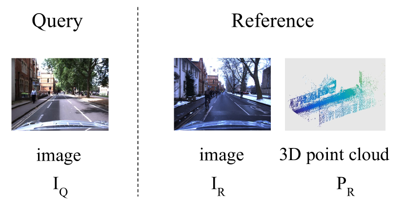
Fig. 1: Inputs for the pose estimation methods in the simplest scenario: a query image $I_{Q}$ and a reference tuple $(I_{R},P_{R})$, where $I_{R}$ is a single reference image and $P_{R}$ is the registered 3D point cloud associated to $I_{R}$. Both the the point cloud $P_{R}$ and the camera pose of the reference image $I_{R}$ are defined in a common world coordinate system.

2.1 Indirect feature-based (FB) pose estimation

A standard feature-based pose estimation method can be divided into four main steps: $(1)$ feature detection, $(2)$ feature matching, $(3)$ 2D-3D correspondences grouping, and $(4)$ Perspective-n-Point pose estimation. The block diagram of this method is shown in Fig. 2. In the first step, a feature detector and a feature descriptor are applied to both query and reference images to find interest-points or regions and form their descriptors from pixels surrounding each detected region. Secondly, based on the descriptors of the feature points, 2D-2D correspondences are sought between query and reference images with a feature matcher. Thirdly, since the 3D point cloud is registered with the reference image, the 2D-3D correspondences between the query image and the 3D point cloud can be computed through the 2D-2D correspondences between the query and reference image. Finally, a Perspective-n-Point solver (Gao et al., 2003) and RANSAC (Fischler and Bolles, 1981; Torr and Zisserman, 2000) are applied for computing the 6-DoF camera pose of the query image. The algorithm and implementation details of each stage of the feature-based pose estimation can be found in A.

Fig. 2: Block diagram of feature-based camera pose estimation. $I_{Q}$ is the query image. The reference image $I_{R}$ and the 3D point cloud $P_{R}$ are pre-registered and defined in the world coordinate system. $\textbf{M}^{*}$ is the estimated transformation matrix. For the detailed descriptions of each step see A.

2.2 Direct photometric-based (PB) pose estimation

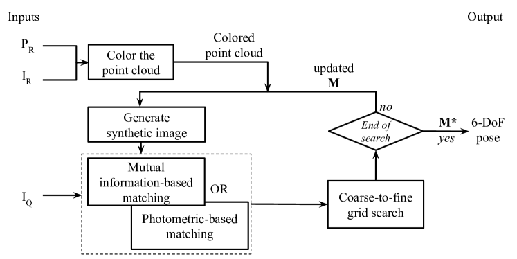
Fig. 3: Block diagram of direct photometric-based and mutual information based camera pose estimation. $I_{Q}$ is the query image. The reference image $I_{R}$ and the 3D point cloud $P_{R}$ are pre-registered and defined in the world coordinate system. $\textbf{M}^{*}$ is the estimated transformation matrix. For the detailed descriptions of each step see B.

Fig. 4: Block diagram of hybrid approach of camera pose estimation. $I_{Q}$ is the query image. The reference image $I_{R}$ and the 3D point cloud $P_{R}$ are pre-registered and defined in the world coordinate system.

The direct photometric-based approach (Tykkälä et al., 2013) is defined as a direct minimization of the cost function at the space of 6D camera pose, and it does not need to extract local features. The pixel intensities of the query image and rendered synthetic view from the 3D point cloud are directly compared in the cost function (Tykkälä et al., 2013). The photometric-based approach can be divided into three main steps: $(1)$ synthetic image generation, $(2)$ photometric matching, and $(3)$ coarse-to-fine search.

The block diagram of this method is shown in Fig. 3. In summary the algorithm works as follows: firstly, for rendering a colored 3D point cloud must be generated. This is generated by projecting each 3D point of the cloud $P_{R}$ to the reference image frame and then assigning colors from the points of the reference image at that location. Subsequently, we generate a synthetic image by projecting the colored 3D point cloud into an image plane, where the transformation matrix of the reference image is used as the initial matrix. Then, we optimize the transformation matrix M by a grid search. In the end, the 6-DoF camera pose is obtained from the final transformation matrix $\textbf{M}^{*}$. It should be noted that in common tracking applications where transformation baseline is small, fast optimization can be implemented by using Jacobian and gradient-based optimization (Tykkälä et al., 2013). However, in the case of big appearances changes between the query and references images, the gradient tends to go to local minimum, so we conduct a grid search in our experiment.

A more detailed description of the stages and implementation details of the photometric-based pose estimation method can be found in B.

2.3 Direct mutual-information-based (MI) pose estimation

The direct mutual-information-based approach (Pascoe et al., 2017) is a direct method similar as the photometric-based pose estimation, and it has more robust similarity measurements. Because the above described direct photometric-based pose approach is sensitive to photometric changes, e.g. due to illumination change. To compensate these effects, a more robust similarity measure – Mutual Information (MI) (McDaid et al., 2011) – that can be used to replace the direct pixel-based photometric-error in the pose estimation cost function. The mutual information is the measure of the mutual dependence between two variables and can be used over different modalities, and mutual-information-based image registration approaches are widely used in medical image registration over different modalities (Mani and rivazhagan, 2013). In turn, the normalized mutual information has the advantage that its values are in the bounded range of $[0,1]$  (McDaid et al., 2011).

The direct mutual-information-based approach is similar to the direct photometric-based pose approach in Section 2.2, with the main difference being that in the cost function the normalized mutual information (NMI) is used instead of the photometric error (see Fig. 3). Specifically, mutual information based pose estimation is formulated as a minimization problem as:

$$\textbf{M}^{*}=\arg\min_{\textbf{M}}1-\textit{NMI}(I_{Q},I_{S}),$$ (1)

where $\textbf{M}^{*}$ is the estimated camera pose, $I_{Q}$ is the query image, $I_{S}$ is the synthetic image for which the generation process is described in B.1, and the Normalized Mutual Information (NMI) is computed as:

$$\textit{NMI}(I_{S},I_{Q})=\dfrac{\textit{MI}(I_{S},I_{Q})}{max(H(I_{S}),H(I_{Q}))}\enspace$$ (2)

with

$$MI(I_{S},I_{Q})=H(I_{S})+H(I_{Q})-H(I_{S},I_{Q})\enspace,$$ (3)

where $H(I_{S},I_{Q})$ is the joint entropy of $I_{S}$ and $I_{Q}$, $H(I_{S})$ and $H(I_{Q})$ are the marginal entropies of $I_{S}$ and $I_{Q}$, and $MI(I_{S},I_{Q})$ is the mutual information between $I_{S}$ and $I_{Q}$.

2.4 Hybrid (HY) pose estimation

The hybrid approach for camera pose estimation takes the advantages of both indirect feature-based pose estimation and direct mutual-information-based pose estimation. This method is inspired by the strong empirical evidence in our experiments that: (1) the feature-based method is superior in accuracy if a sufficient number of matches can be found (see detail at Section  4.3 and 4.5); (2) the feature-based approach can completely fail where mutual-information-based approach can still provide a moderate estimate. Therefore, our hybrid approach first executes the feature-based method and if that fails ($<4$ consistent 2D-3D correspondences) (Torr and Zisserman, 2000; Gao et al., 2003), then switches to the MI-based method.

Given one query image $I_{Q}$ and one reference tuple $(I_{R},P_{R})$ (see definition at Fig. 1 and Section  2), a feature detector is firstly applied to both the query image $I_{Q}$ and reference image $I_{R}$ , and then we apply feature matching to get 2D-2D matched features. Since the point cloud $P_{R}$ is registered with the reference image $I_{Q}$, the 2D-3D correspondences can be found. Then a PnP solver (Gao et al., 2003) and RANSAC (Torr and Zisserman, 2000) are applied to the 2D-3D correspondence. For the PnP solver (Gao et al., 2003), at least 4 consistent 2D-3D correspondences pairs are required. If the camera pose of the query image cannot be estimated due to less than 4 2D-3D correspondences (Torr and Zisserman, 2000; Gao et al., 2003), the direct mutual-information-based pose estimation is adopted to compute the camera pose. The block diagram of the hybrid approach is shown in Fig. 4.

3 Comparative methodology

In this work, we systematically compare camera pose estimation approaches in three stages: firstly, we compare the performance of different pose estimation methods for single query image in the simplest scenario by using one reference tuple, defined in Fig.1 (methodology in Section 3.1 and experimental results in Section 4.3). Secondly, we increase the number of reference images and evaluate the improvement in accuracy for the studied approaches (methodology in Section 3.2 and experimental results in Section 4.4). Thirdly, we evaluate the different approaches with large uncertainties, where the reference images and their corresponding 3D point clouds can be far away from the query image (methodology in Section 3.3 and experimental results in Section 4.5).

3.1 Single-reference pose estimation

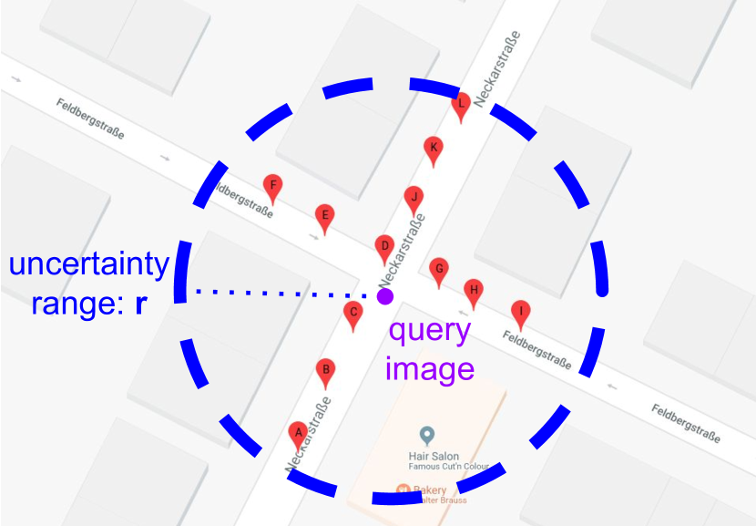
Fig. 5: This is the visualization of how a reference image is selected for camera pose estimation in Section 3.1. The ground truth position of the query image is marked with a purple dot, and a circle around the purple dot represents the initial uncertainty of the query image’s location. Within the initial uncertainty circle, one reference image is randomly selected among all possible candidates that are indicated with red markers from A to L.

The aim of using a single reference image for different pose estimation methods is to compare their performance at the most basic level without pre- or post-processing steps. As illustrated in Fig. 5, the experiment starts by firstly defining a uncertainty range with a radius of $r$ around the ground truth location of the query image, and $r$ represents the initial uncertainty of the query image’s location. In this paper, initial uncertainty value $r$ is given by the author and it determines the region where the possible reference images can be chosen from. The reference image is randomly selected in the region within the circle, and the aim of introducing the random selection is to evaluate how the studied algorithms respond to different displacements between the query and reference images, because one concern about the performance of pose estimation methods is the need of a proper initialization (i.e., a good estimate of the current camera location). Therefore, After randomly selecting one reference image within the radius, the inputs of the single-reference case are the query image $I_{Q}$ and a reference tuple $(I_{R},P_{R})$, where where $I_{R}$ is a single reference image and $P_{R}$ is its corresponding 3D point cloud (an example of reference tuple is shown in Fig.1). The quality of the estimated pose is then assessed in terms of the translation error and rotation error (see Section 4.2).

3.2 Multiple-reference pose estimation

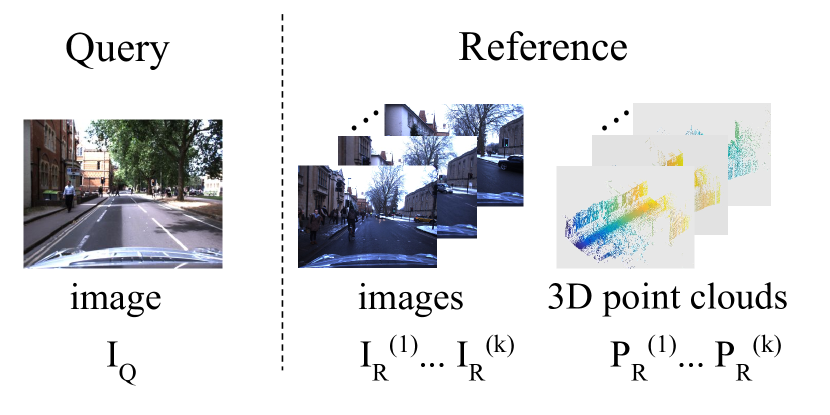
Fig. 6: Example of inputs for multi-references case: one query image $I_{Q}$ and multiple reference tuples $\{(I_{R}^{(1)},{P_{R}}^{(1)}),\ldots(I_{R}^{(k)},{P_{R}}^{(k)})\}$ which consist of $k$ reference images and $k$ 3D point clouds.

In this section we explain the case of incorporating the information obtained from multiple reference images to estimate the camera pose of a single query image. Therefore, the inputs are one query image and multiple reference tuples which consist of $k$ pairs of reference images and their corresponding 3D point clouds, $\{(I_{R}^{(1)},{P_{R}}^{(1)}),\ldots(I_{R}^{(k)},{P_{R}}^{(k)})\}$, as shown in Fig. 6. The aim of using multiple reference images is to leverage the additional information of different reference images to improve accuracy of the camera pose estimation.

In the prior art, Song et al. (2016) fuse multiple candidate camera poses by: (1) averaging three rotation angles to compute the final rotation matrix; (2) minimizing a geometry error term to estimate the final translation. However, 3D point clouds are not utilized in their approach, so from each of their candidate camera pose only a line where the camera pose of the query image should lie on is obtained. In contrast, in our approach, each reference image together with the 3D point clouds are already sufficient to compute a unique 6-DoF camera pose for the query image. Therefore, we have considered 4 strategies, which can be easily adapted to different camera pose estimation methods.

1. Maximum number of matched features (maxf): we match the query image with all the available reference images, and select the reference image with the most matched features after the feature matching stage (Section A.2). Then, we compute the camera pose of the query image with only the reference tuple contains the selected reference image. The remaining processing steps are the same as in the camera pose estimation with single reference tuple (see Section 2).

2. Simple average (avg): for each reference tuple in $\{(I_{R}^{(1)},{P_{R}}^{(1)}),\ldots(I_{R}^{(k)},{P_{R}}^{(k)})\}$ , we compute an individual candidate camera pose as described in Section 2. As a result, $k$ candidate camera poses will be obtained. Each 6-DoF camera pose consists of a rotation matrix and a translation vector. We average the $k$ rotation matrices by firstly converting them to quaternions and then apply quaternion space interpolation (Markley et al., 2007). As a result, the final rotation matrix is obtained from the interpolated quaternion, and the final translation vector can be computed by averaging all the translation vectors.

3. Weighted average (wavg): similarly as simple average, this approach starts with $k$ individual candidate camera pose estimates obtained from each reference tuple. Then we take a weighted average of these $k$ camera poses, and the weights are computed according to the number of the matched features between the query image and each reference image.

4. Robust weighted average (r-wavg): firstly we match the query image with all the available reference images and record the numbers of their matches. If the maximum number of matches is $K$ between the query and each reference image, we select those reference images with at least half of the maximum matches $K/2$. Then, we use them to compute the individual candidate camera poses and apply the weighted average over them.

3.3 Camera pose estimation with large uncertainties

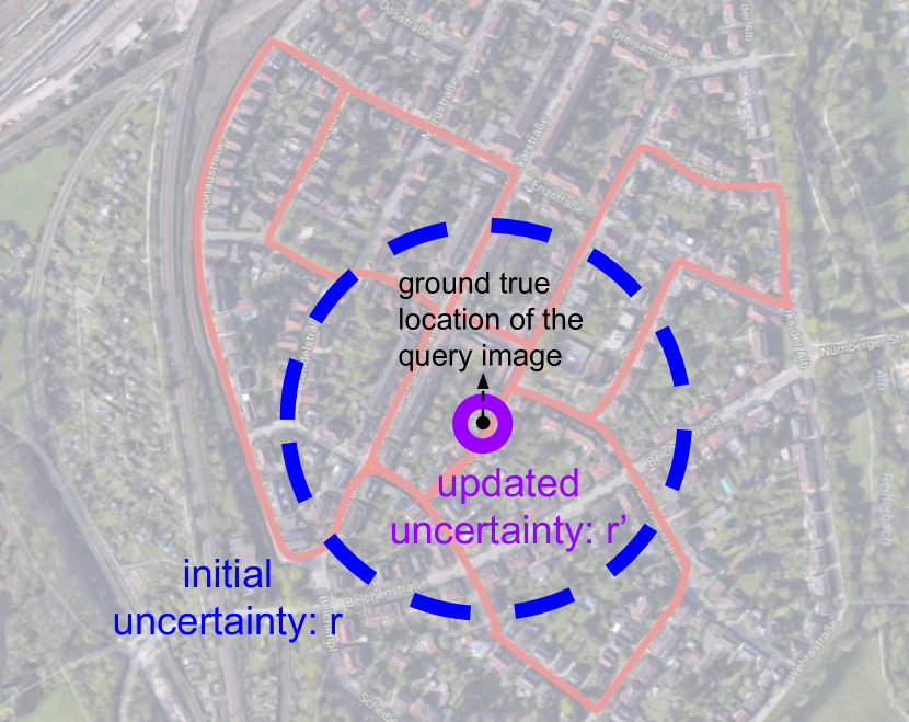
Fig. 7: It is a visualization of applying an image retrieval method and a camera pose estimation method to reduce the large position uncertainty of the query image. The black dot represents the ground true location of the query image, the big blue dashed circle shows the initial uncertainty and the small purple solid circle indicates the updated uncertainty after processing. The red route marked in the background is one of the KITTI dataset route.

In real-life applications, the query image may or may not have a GPS tag, and even with a GPS tag, the precision of the GPS can be poor (Linegar et al., 2016; Miura et al., 2015). Therefore, the initial uncertainty radius $r$ of the query camera’s location can be as large as shown in Fig. 7. In the case of large uncertainty, choose the reference image by random selection is not practical anymore, but the use of image retrieval methods is a widely accepted practice. Therefore, we compare the performances of the studied pose estimation methods with large uncertainty, and evaluate how image retrieval improves their performance.

Specifically, for the case of the query image with large initial uncertainty, image retrieval methods such as (Song et al., 2016; Philbin et al., 2007; Radenović et al., 2016; Iscen et al., 2017) are used to effectively identify a few good reference images from the reference database. To replicate this procedure we selected the method by (Philbin et al., 2007) which is easy to implement and performs the image retrieval task with large scale data by quantizing low-level image features based on randomized trees and using an efficient spatial verification stage to re-rank the results returned from our bag-of-words model. Furthermore, we apply all evaluated camera pose estimation methods with multiple reference images to compute the final 6-DoF camera pose.

4 Experiments and results

4.1 Datasets

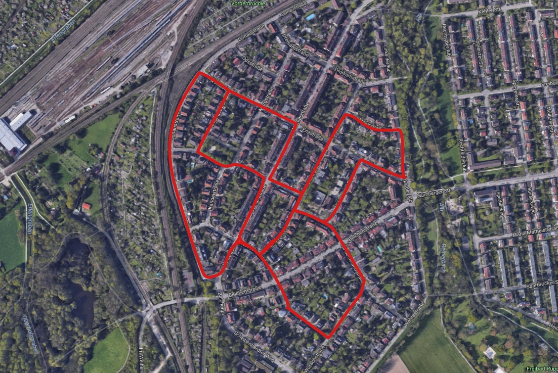
Fig. 8: The route of sequence 00 in Table 1 (KITTI dataset).

In this work, experiments were conducted using two public datasets: the KITTI Visual Odometry dataset (Geiger et al., 2012) and the Oxford RobotCar dataset (Maddern et al., 2017).

The KITTI dataset was captured by driving around the mid-size city of Karlsruhe (Germany), in rural areas and on highways. The accurate ground truth is provided by a Velodyne laser scanner and a GPS localization system. There are 11 sequences in KITTI Visual Odometry dataset with provided ground-truth camera pose, and we use all of them in our experiments. All 11 sequences are summarized in Table 1. For each sequence, 3D point cloud $P_{R}$ is obtained from the provided LIDAR data, and both query image $I_{Q}$ and reference image $I_{R}$ are from one monochrome camera (according to the author the monochrome camera is less noisy). One example of the sequence route for KITTI dataset is shown in Fig. 8;

Table 1: Overview of the 11 sequences in the KITTI dataset (Geiger et al., 2012).

id	# images	tag	total length (km)	mean distance between consequent images (m)
00	4541	urban	3.7	0.8
01	1101	highway	2.5	2.2
02	4661	urban	5.1	1.1
03	801	urban	0.6	0.7
04	271	urban	0.4	1.5
05	2761	urban	2.2	0.8
06	1101	urban	1.2	1.1
07	1101	urban	0.7	0.6
08	4071	urban	3.2	0.8
09	1591	urban	1.7	1.1
10	1201	urban	0.9	0.8

The recently released Oxford RobotCar dataset (Maddern et al., 2017) provides multiple traversals of the same route and allows a more challenging evaluation in extreme changing conditions, e.g. different time of the day, lighting and weather condition. 5 sequences of the Oxford RobotCar dataset with completely different environment conditions were selected for our experiments. The sequence route is shown in Fig. 9 and example images from 5 sequences are shown in Fig. 10. Similar to KITTI dataset, 3D point cloud $P_{R}$ is from 3D LIDAR data, and query image and reference images are image taken from different traversals. The reported GPS information is treated as the ground-truth. For efficiency, we reduced the number of images in each sequence by taking 1 image out of every 10 images and removed the beginning and ending frames of each sequence where the car is usually parked resulting same views all the time. The resulting 5 sequences from Oxford RobotCar dataset are summarized in Table 2. In the case of Oxford dataset the query $I_{Q}$ and reference $I_{R}$ images are taken from different traversals, and therefore give much more realistic picture of pose estimation performance in real applications.

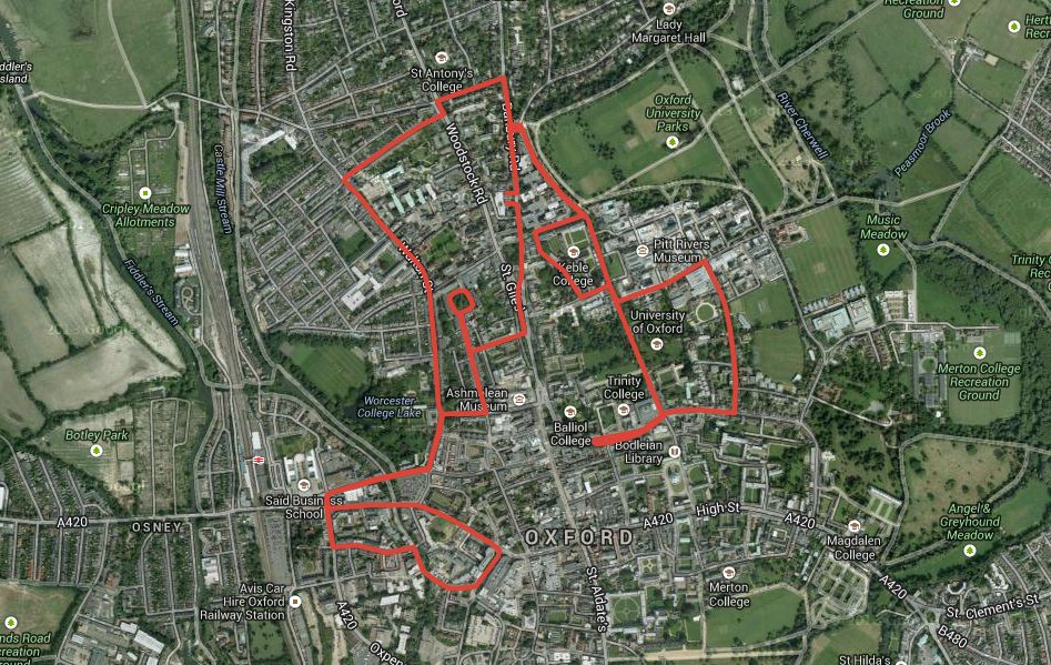
Fig. 9: The route used for all 5 sequences in Table 2 (Oxford RobotCar dataset).

Table 2: Overview of 5 sequences with different environmental conditions in Oxford RobotCar dataset (Maddern et al., 2017).

id	# images	tag	total length (km)	mean distance between consequent images (m)
00	1916	overcast	6.3	3.3
01	2873	sun	8.6	3.0
02	2931	night	9.1	3.1
03	2614	rain	8.8	3.4
04	3019	snow	8.7	2.9

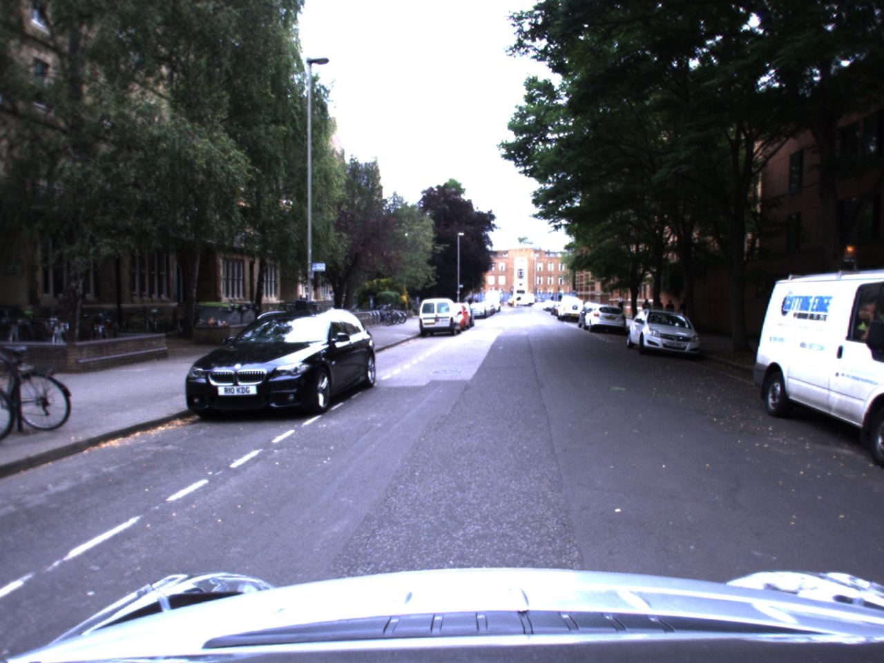
(a) overcast

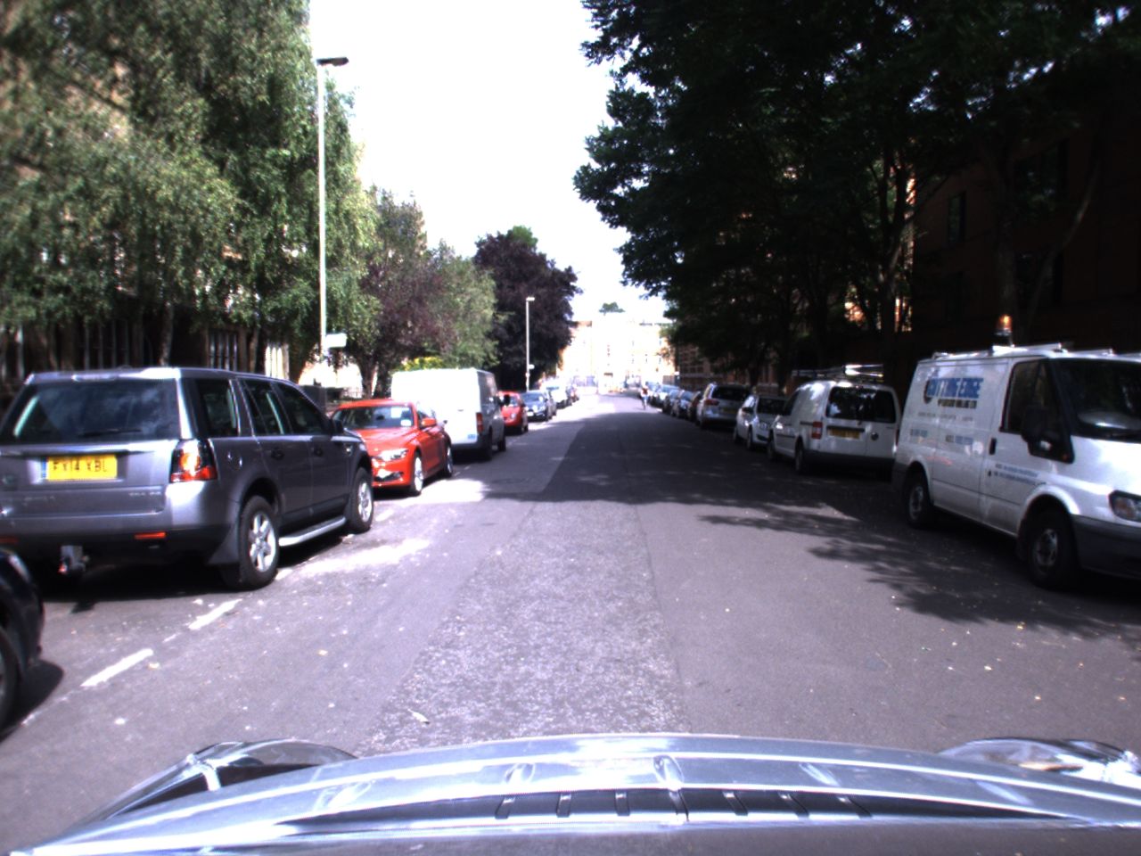
(b) sun

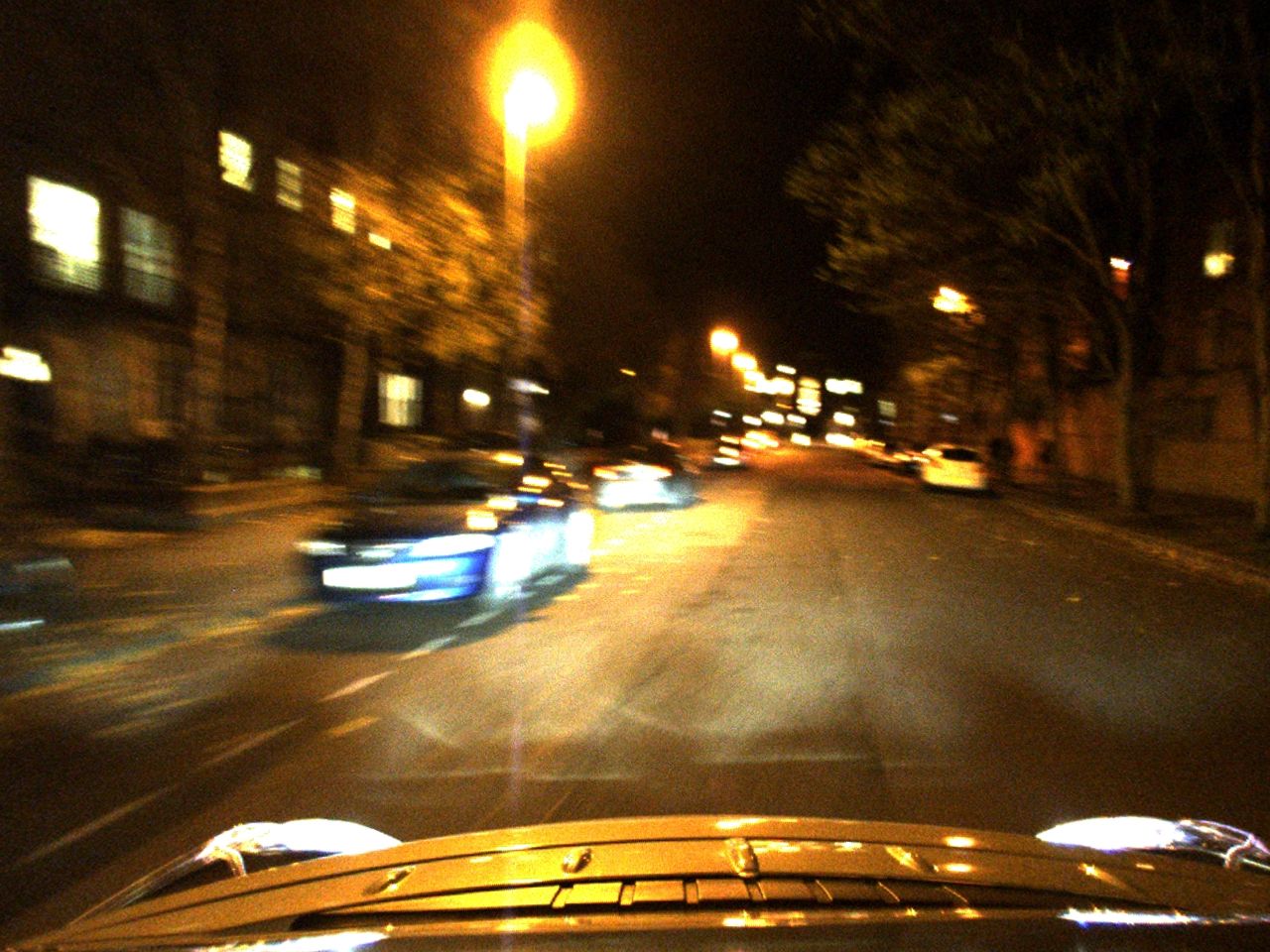
(c) night

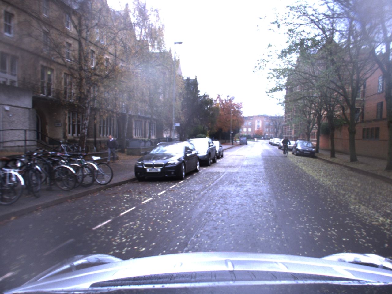
(d) rain

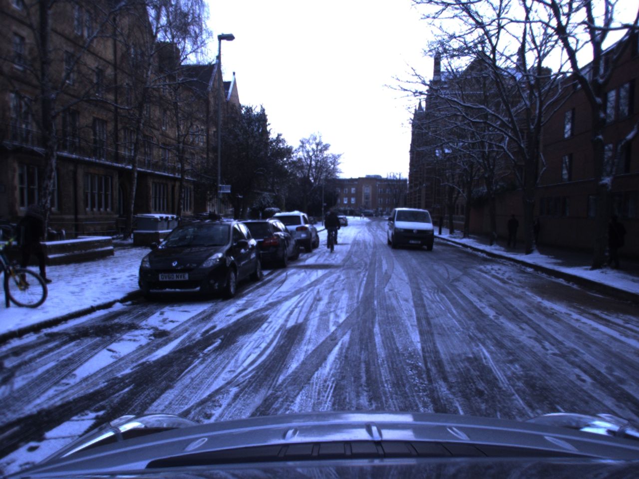
(e) snow

Fig. 10: Appearance differences among the 5 sequences in Table 2 (the images are roughly from the same location).

4.2 Performance measures

We use translation error, maximum orientation error and the success rate of each methods to compare the performance of the different approaches.

1. The translation error is the absolute translation between the ground-truth location and the estimated location of the query image.

2. Based on the rotation matrix between the ground-truth camera pose and the estimated camera pose of the query image, we convert the rotation matrix into 3 Euler angles. Then the maximum absolute Euler angle is used as the maximum orientation error.

3. Different camera pose estimation methods can fail to estimate a 6-DoF camera pose of the query image under some circumstances, e.g. no enough feature matches between the query and reference images in indirect feature-based approach, or searching cannot converge within given search ranges in direct photometric-based approach. We classify the pose estimation failure as either self-reported by each method or the translation errors are greater than a predefined threshold (see details in the each experiment). The success rate of each methods is the percentage of the successfully processed query images with an valid camera pose as the output.

4.3 Experiments with single reference image

We performed 12 experiments for KITTI dataset and 12 experiments for Oxford RobotCar dataset. The goal of these experiments was to compare the performance of different pose estimation methods under the single reference scenario. In Section 3.1, we discussed the camera pose estimation for one query image $I_{Q}$ with single reference tuple $(I_{R},P_{R})$ where $I_{R}$ is a single reference image and $P_{R}$ is its corresponding 3D point cloud. Similarly, we firstly gathered all reference images within the uncertainty radius $r$ around the given query image’s GPS location, and $r$ was varied between 10 to 25 meters, since most of the photos are taken in the streets of urban area, and these search ranges were used so that the reference image and query images would have some overlaps but without being too close to each other. Within the gathered reference images, we applied random selection to choose one reference image $I_{R}$ and its corresponding 3D point cloud $P_{R}$. The reasons for using random selection is to evaluate how the studied algorithms respond to different displacements between the query and reference images (i.e., different initializations).

The experiments with KITTI dataset tested the performance of different camera pose estimation methods under “ideal conditions”, i.e. same time of the day, lighting and weather condition. For the KITTI dataset listed in Table 1, all 11 sequences have different routes, so each sequence was processed individually. In other words, the query image and the reference images come from the same drive. In order to separate the query and reference images, we randomly selected 10% of the images in one sequence as query images, and the rest images from the same sequence were used as reference images.

The experiments with Oxford RobotCar dataset tested the performance of camera pose estimation methods at challenging conditions since the query and reference data capture large variation in appearance and structure of a dynamic city environment over long periods of time. For the Oxford RobotCar dataset presented in Table 2, all 5 traversals with complete different environment settings share the same route. The sequences were processed jointly in order to allow the query and reference images come from the different sequences. For example, when the summer sunny sequence (01 in Table. 2) was used for the reference images, the winter snow sequence (04 in Table. 2) was used for the queries.

Table 3 shows the translation errors and orientation errors of different pose estimation methods by using a single reference image. The results are reported in median values, and both the translation and orientation errors are calculated based on the estimates obtained by the studied methods and the ground-truth camera poses. The success rate of each pose estimation method with Oxford RobotCar and KITTI datasets are shown in Fig. 11.

The main findings are that (1) the indirect feature-based method (FB) is more accurate than direct photometric-based (PM) and mutual-information-based (MI) approaches as long as there are at least 4 consistent 2D-3D correspondences (4 is the minimum number of feature matches required to compute the camera pose by the PnP solver (Gao et al., 2003)); (2) but for the realistic Oxford RobotCar dataset, the success rate of feature-based method (FB) is clearly inferior to mutual-information-based method (MI). Note that full analysis of the results is postponed to the discussion section (Section 5).

Table 3: Translation error (in meters) and max orientation error (in degrees) comparison for three strategies using single reference image. For KITTI dataset, 454 images (random 10% of the whole sequence) in sequence 00 are use as queries, and the rest are used the reference images. For Oxford RobotCar dataset, summer sequence (01) is used as references and 302 images (random 10% of the winter sequence) from winter sequence are used as query images. Second row shows the number of images which are successfully processed by all three pipelines. Third row shows the percentage of the successfully processed images among all the testing images.

(a) KITTI sequence: translation error (m)

uncertainty radius (m)	10	15	20	25
#images	406	328	282	259
	(89%)	(72%)	(62%)	(57%)
FB (Kim et al., 2014)	0.13	0.40	0.48	0.30
PM (Tykkälä et al., 2013)	1.44	6.66	7.77	14.85
MI (Pascoe et al., 2017)	1.56	5.41	6.15	10.26

(b) Oxford sequence: translation error (m)

uncertainty radius (m)	10	15	20	25
#images	67	60	53	38
	(22%)	(20%)	(18%)	(13%)
FB (Kim et al., 2014)	2.77	2.48	2.40	2.91
PM (Tykkälä et al., 2013)	10.44	16.23	20.09	26.32
MI (Pascoe et al., 2017)	8.71	13.36	16.27	14.94

(c) KITTI sequence: max orientation error (degree)

uncertainty radius (m)	10	15	20	25
#images	406	328	282	259
	(89%)	(72%)	(62%)	(57%)
FB (Kim et al., 2014)	1.76	3.83	5.42	3.33
PM (Tykkälä et al., 2013)	1.07	2.40	3.37	3.12
MI (Pascoe et al., 2017)	1.07	2.30	3.45	2.70

(d) Oxford sequence: max orientation error (degree)

uncertainty radius (m)	10	15	20	25
#images	67	60	53	38
	(22%)	(20%)	(18%)	(13%)
FB (Kim et al., 2014)	3.44	3.79	2.72	3.25
PM (Tykkälä et al., 2013)	3.48	5.82	2.64	1.88
MI (Pascoe et al., 2017)	6.16	4.00	2.42	1.93

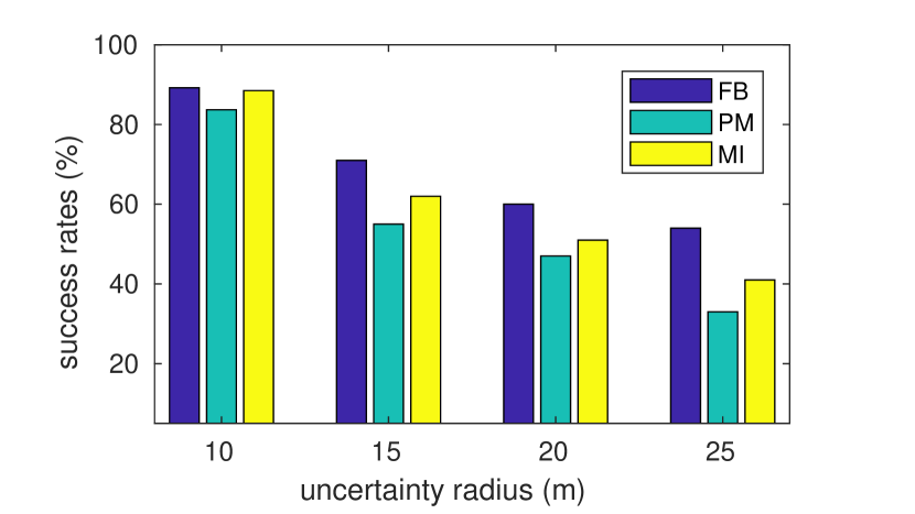
(a) KITTI

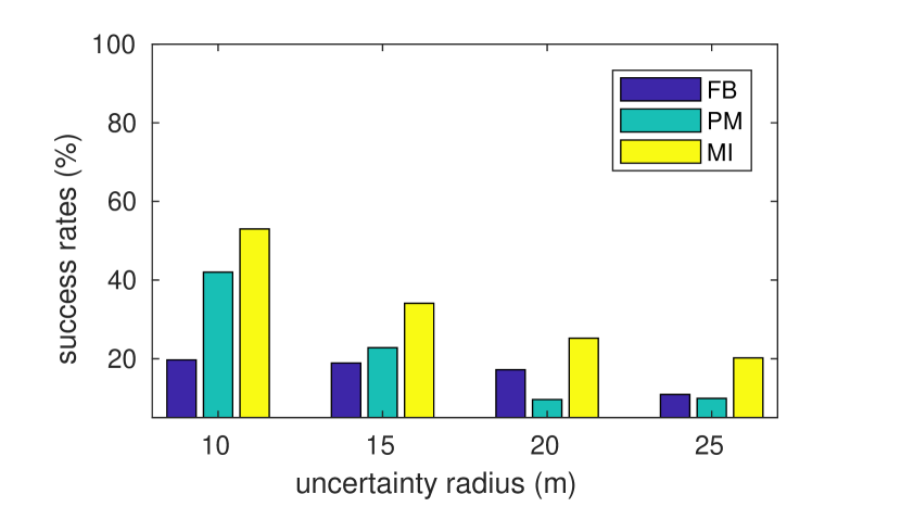
(b) Oxford RobotCar

Fig. 11: Success rate comparison for three strategies with single reference image at different uncertainty ranges in two public datasets. (a): in the experiments with KITTI sequence 00, random 10% images in sequence 00 are used as query image and the rest are used as references. (b): in the experiments with two sequences in Oxford RobotCar sequences, summer sequence (01) is used as references and snow sequence (04) is used as query images.

4.4 Experiments with multiple references images

In this experiment, we evaluated the performance of different methods in the multiple reference images setting for the both KITTI and Oxford RobotCar dataset. The goal was to find efficient ways to incorporate the information obtained from multiple reference images to improve the camera pose estimation.

Similar to the single reference image case in Section 4.3, we first gathered the reference images within a given uncertainty radius $r$ around the query image’s GPS, and then randomly selected multiple reference tuples. Subsequently, we used 4 different methods to estimate camera poses with multiple reference tuples: maximum number of matched features (maxf), simple average (avg), weighted average (wavg) and the robust weighted average (r-wavg). The number of reference images was varied from one to five.

The comparison of different multiple-references pose estimation methods with KITTI dataset are shown in Table 4. Fig. 12 compares the success rates for different camera pose estimation methods with multiple reference images using the robust weighted average (r-wavg) method in both KITTI and Oxford RobotCar datasets. The r-wavg method was used since it yielded the best overall performance for all the pose estimation methods.

The main findings of this experiment are that (1) the r-wavg method outperforms other fusion strategies (Table 4), and (2) feature-based approach is the most accurate in terms of both translation accuracy and orientation accuracy (Table 4). Again, the results are collectively summarized in the discussion section (Section 5).

Table 4: Performance of 4 pose merge methods used by each camera pose estimation approach in KITTI dataset. 10% images from one sequence are used as query image and the rest are used as references, and uncertainty radius is 10 meters. The reported results are computed from all processed images by each camera pose estimation approach.

#reference images	1		2		3		4		5
	RMSE (m)	RMSE (deg)	RMSE (m)	RMSE (deg)	RMSE (m)	RMSE (deg)	RMSE (m)	RMSE (deg)	RMSE (m)	RMSE (deg)
Feature-based (FB)
avg	0.125	1.76	0.216	2.07	0.248	2.20	0.212	1.80	0.195	1.61
wavg	0.125	1.76	0.148	1.67	0.151	1.78	0.103	1.22	0.090	1.11
maxf	0.125	1.76	0.106	1.82	0.093	1.79	0.060	1.21	0.049	1.03
r-wavg	0.125	1.76	0.117	1.70	0.104	1.59	0.059	1.13	0.045	0.93
Photometric (PM)
avg	1.67	1.22	2.39	1.36	2.20	1.42	2.09	1.23	1.90	1.05
wavg	1.67	1.22	1.79	1.08	1.55	1.07	1.29	0.80	1.12	0.70
maxf	1.67	1.22	1.37	1.07	1.22	1.02	1.20	0.73	1.07	0.67
r-wavg	1.67	1.22	1.40	1.01	1.22	0.87	1.12	0.68	0.99	0.58
Mutual Information (MI)
avg	1.75	1.35	1.71	1.28	1.84	1.46	1.69	1.25	1.61	1.13
wavg	1.75	1.35	1.51	1.14	1.39	1.21	1.17	0.79	1.18	0.78
maxf	1.75	1.35	1.43	1.10	1.29	1.06	1.17	0.80	1.13	0.68
r-wavg	1.75	1.35	1.43	1.07	1.26	0.95	1.10	0.69	1.03	0.62

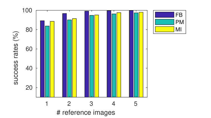
(a) KITTI

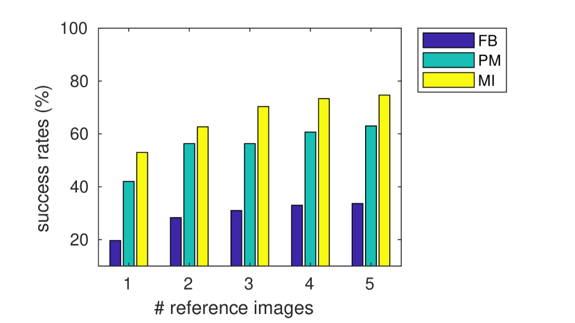
(b) Oxford RobotCar

Fig. 12: Success rates comparison for three pipelines with multiple reference images and robust weighted average merge method in two datasets.

4.5 Experiments at large uncertainty

Based on the strong empirical results in Section 4.3, we proposed a hybrid approach that takes the advantages of both the feature-based and the mutual-information-based approaches as described in Section 2.4. In this Section, we tested these 4 camera pose estimation methods (feature-based, photometric-based, mutual-information-based, and hybrid approaches) with maximum 5 reference images under large uncertainty condition.

In Section 3.3, we introduced a framework for camera pose estimation under large location uncertainty. In the extreme case this means that no prior location estimate is available, but the query image must be matched to the whole reference database, so a image retrieval method (Philbin et al., 2007) is applied to find the reference images. In our experiment we used 200 meters as the initial uncertainty radius for the KITTI and 50 meters for the Oxford dataset, adopted the multiple reference (up to 5 reference images) to improve robustness of all investigated methods. The KITTI dataset correspond to an “ideal case” where query images and references images are from the same environmental setting, while Oxford RobotCar dataset represents results for a more realistic case where the query and references images have completely different environmental setting. We report results for all 11 KITTI sequences, and a 100-fold experimental results for the Oxford RobotCar dataset where one sequence used as the reference dataset and other sequences as the query dataset.

The results for the 11 KITTI sequences are shown in Table 5. This table consists of 44 experiments, each of the 11 sequence in KITTI dataset processed by the four camera pose estimation methods. The uncertainty radius was set to be 200 meters, the maximum number of reference images was set to 5, and we classify the localization failure as either system-reported or $\geq$ 10 meters absolute translation error. The results for the Oxford RobotCar dataset are shown in Table 6. The uncertainty radius was set to be 50 meters, the maximum number of reference images was set to 5, and we classify the localization failure as either system-reported or 20 meters absolute translation error.

The most interesting finding of these experiments is that our hybrid method that combines the complementary properties of the feature-based and mutual information based approaches is the most effective and robust for all query-reference pairs with the difficult and realistic Oxford dataset. The detailed analysis is presented the discussion Section 5.

Table 5: Large uncertainty pose estimation results for 11 sequences in the KITTI dataset combining image retrieval and pose estimation. The uncertainty radius is 200 meters and the number of automatically retrieved reference images is 5. Note these two original papers (Tykkälä et al., 2013; Pascoe et al., 2017) were designed for slam problem, but we modified the algorithms to adjust to our problem.

#sequence ID	00			01			02			03
	%	RMSE (m)	RMSE (deg)	%	RMSE (m)	RMSE (deg)	%	RMSE (m)	RMSE (deg)	%	RMSE (m)	RMSE (deg)
FB (Kim et al., 2014)	99.8	0.031	0.676	84.5	0.494	0.567	99.8	0.025	0.415	100	0.015	0.370
PM (Tykkälä et al., 2013)	98.2	0.603	0.423	76.4	1.208	0.343	92.9	0.550	0.324	98.8	0.342	0.279
MI (Pascoe et al., 2017)	97.8	0.633	0.415	60.0	0.980	0.353	97.6	0.475	0.327	98.8	0.270	0.223
HY (proposed)	99.8	0.031	0.676	89.1	0.505	0.562	99.8	0.025	0.415	100	0.015	0.370
#sequence ID	04			05			06			07
	%	RMSE (m)	RMSE (deg)	%	RMSE (m)	RMSE (deg)	%	RMSE (m)	RMSE (deg)	%	RMSE (m)	RMSE (deg)
FB (Kim et al., 2014)	100	0.028	0.132	100	0.022	0.472	100	0.029	0.421	100	0.018	0.326
PM (Tykkälä et al., 2013)	96.3	0.783	0.222	97.8	0.514	0.360	98.2	0.382	0.308	97.3	0.505	0.336
MI (Pascoe et al., 2017)	100	0.495	0.177	97.1	0.537	0.352	96.4	0.551	0.332	98.2	0.500	0.319
HY (proposed)	100	0.028	0.132	100	0.022	0.472	100	0.029	0.421	100	0.018	0.326
#sequence ID	08			09			10
	%	RMSE (m)	RMSE (deg)	%	RMSE (m)	RMSE (deg)	%	RMSE (m)	RMSE (deg)
FB (Kim et al., 2014)	100	0.018	0.383	99.4	0.019	0.356	100	0.019	0.420
PM (Tykkälä et al., 2013)	97.3	0.499	0.329	95.0	0.548	0.321	94.2	0.634	0.355
MI (Pascoe et al., 2017)	95.3	0.518	0.341	93.7	0.400	0.350	91.7	0.780	0.343
HY (proposed)	100	0.018	0.383	100	0.019	0.368	100	0.019	0.420

Table 6: Large uncertainty pose estimation results for the 5 different sequences in Oxford dataset (5-fold experiment where each sequence was paired with each sequence to form query-reference pairs). The uncertainty radius was set to 50 meters and the number of automatically retrieved reference images was 5. The failure threshold was set to 20 meters. Note these two original papers (Tykkälä et al., 2013; Pascoe et al., 2017) were designed for slam problem, but we modified the algorithms to adjust to our problem..

		overcast			sun			night			rain			snow
		%	RMSE	RMSE	%	RMSE	RMSE	%	RMSE	RMSE	%	RMSE	RMSE	%	RMSE	RMSE
			(m)	(deg)		(m)	(deg)		(m)	(deg)		(m)	(deg)		(m)	(deg)
overcast	FB (Kim et al., 2014)	98.4	0.111	0.791	32.7	3.309	3.070	6.0	6.441	4.200	30.7	3.491	5.029	17.0	1.505	7.068
	PM (Tykkälä et al., 2013)	100.0	1.601	0.568	28.8	14.389	9.250	23.2	14.283	19.964	22.2	12.004	4.122	21.6	12.202	8.342
	MI (Pascoe et al., 2017)	100.0	1.577	0.726	41.6	11.603	7.945	43.8	13.077	12.788	37.3	13.523	12.607	44.3	11.594	8.918
	HY (proposed)	100.0	0.112	0.788	57.2	4.366	6.840	47.6	12.470	9.867	55.1	5.672	8.112	52.3	8.124	8.360
sun	FB (Kim et al., 2014)	34.0	2.615	2.122	98.3	0.121	0.706	3.3	5.104	14.612	13.6	2.982	4.482	16.6	2.970	4.820
	PM (Tykkälä et al., 2013)	30.7	11.482	6.946	99.7	2.035	0.597	31.5	12.904	10.508	25.3	12.819	8.778	22.8	14.221	5.644
	MI (Pascoe et al., 2017)	44.0	11.908	6.384	99.7	1.770	0.567	40.7	11.246	7.906	35.0	12.007	7.063	40.4	11.754	4.982
	HY (proposed)	56.7	3.478	3.983	99.7	0.122	0.715	41.8	10.584	8.810	44.0	10.225	5.954	48.7	9.569	4.955
night	FB (Kim et al., 2014)	5.9	4.132	3.158	2.5	5.759	16.003	91.1	0.221	0.750	1.2	2.879	4.171	2.7	6.481	8.260
	PM (Tykkälä et al., 2013)	22.5	12.604	11.445	16.1	14.336	17.676	99.3	2.507	0.566	16.3	12.824	11.574	12.7	13.751	19.656
	MI (Pascoe et al., 2017)	31.4	12.698	11.425	34.7	12.035	7.351	99.0	2.247	0.580	37.2	12.382	4.733	32.7	11.899	7.023
	HY (proposed)	36.3	11.334	8.960	35.8	12.004	7.584	99.3	0.238	0.887	37.6	12.236	4.671	33.3	11.381	7.477
rain	FB (Kim et al., 2014)	33.9	3.279	2.908	14.6	2.330	5.389	4.0	2.345	1.505	97.3	0.192	0.767	18.5	3.455	3.844
	PM (Tykkälä et al., 2013)	31.6	11.097	4.481	37.6	12.831	7.472	25.3	12.732	6.548	100.0	2.417	0.610	29.5	13.204	5.913
	MI (Pascoe et al., 2017)	34.5	12.853	9.739	39.0	10.986	6.528	33.3	13.332	8.483	100.0	1.966	1.077	39.1	11.141	6.673
	HY (proposed)	56.1	4.322	5.119	46.7	8.891	7.420	35.9	11.276	7.240	100.0	0.202	0.773	49.0	6.494	5.707
snow	FB (Kim et al., 2014)	10.8	2.556	3.880	11.5	2.731	8.554	2.2	5.733	13.984	11.6	2.622	4.836	97.7	0.145	0.834
	PM (Tykkälä et al., 2013)	18.9	12.768	36.815	16.4	15.801	29.476	20.5	14.563	5.459	12.0	13.549	10.648	100.0	2.200	0.559
	MI (Pascoe et al., 2017)	32.4	11.947	9.698	35.9	12.708	7.956	34.8	12.174	6.299	27.6	12.120	6.223	100.0	2.133	0.731
	HY (proposed)	36.0	9.348	7.545	42.9	10.170	8.480	35.9	11.849	6.278	35.6	9.851	7.310	100.0	0.149	0.804

5 Discussion

5.1 Camera pose estimation with single reference image

Table 3 reports both translation errors and orientation errors comparisons for three strategies using a single reference tuple. In Table 3, the numbers of images in the second line of each sub-table are the number of images that all methods successfully processed and therefore the error numbers are comparable between the methods, and the percentages on the third line of each sub-table are the corresponding percentages of the successfully processed images among the total number of images.

From Table 3(a) and 3(b), we have two findings:

1. By looking into each column, we find that as long as the feature-based approach is able to estimate the camera pose (minimum 4 consistent 2D-3D correspondences are required to compute the camera pose by the PnP method (Gao et al., 2003))), its estimated camera poses have smaller translation errors than the other two methods in both KITTI and Oxford RobotCar dataset. This result indicates that the feature-based approach is more accurate in pose estimation in both ideal environment conditions (KITTI dataset) and realistic environment conditions (Oxford RobotCar dataset).

2. By looking into each row, we find that the translation errors of both photometric-based and mutual-information-based approach increase with the increase of the uncertainty radius, but the translation errors of feature-based approach do not vary much. Since the closer reference images bring better initialization for both the photometric-based and mutual-information-based approach, the results indicate that both the photometric-based and mutual-information-based approach are sensitive to the initialization. However, the feature-based approach is much less sensitive to the location of the reference images.

Table 3(c) and 3(d) compare the orientation errors for the studied methods. Among these different camera pose estimation methods, the differences between their orientation errors are small. In other words, all these methods perform similarly in terms of orientation error for both KITTI and Oxford RobotCar datasets. The reason might be that all the images are taken by a camera mounted on a car driving along the street, so the query images and the reference images may share similar viewpoints.

Fig. 11 records the success rate (see definitions in Section 4.2) comparison for the three strategies with single reference tuple at different uncertainty ranges in two public datasets. Fig. 11 shows the following:

1. By looking at the three bars corresponding to each uncertainty radius, the feature-based approach has higher success rate than the other two approaches in KITTI dataset; however, feature-based approach has the lowest success rate among all three approaches in Oxford RobotCar dataset. The mutual-information-based approach has the highest success rate in Oxford RobotCar dataset. In other words, the success rate of feature-based approach is greatly influenced by the environmental conditions between the query and reference images. On the other hand, the mutual-information-based approach is the most robust in terms of the success rate under different environmental conditions.

2. When analyzing the same pose estimation method for different uncertainty radii, the success rates of all approaches go down with the increase of the uncertainty radius.

The state-of-the-art SLAM approach (Pascoe et al., 2017) claims that the mutual-information-based SLAM approach has higher success rate than the state-of-the-art feature-based SLAM approach (Mur-Artal et al., 2015). Our experiment in Fig. 11(b) provides the same conclusion under the problem of 6-DoF camera pose estimation using single reference image and 3D point cloud. Interestingly enough, our experiments in Table 3 tells that the feature-based approach can be more accurate as long as it is able to compute the camera pose.

5.2 Camera pose estimation with multiple reference images

Table 4 reports the results for the experiments with multiple reference images for three different camera pose estimation methods. The results show that fusing the poses from multi-reference improves the performance of the camera pose estimation results, and robust weighted average (r-wavg) outperforms the other approaches, especially with the increased number of reference images.

Fig. 12 compares the success rates of the different approaches with multiple reference images using robust weighted average method in both KITTI and Oxford RobotCar datasets. Fig. 12 tells us two things:

1. By looking into the success rate of each method, we see that the success rate of different pose estimation methods increases with increasing number of reference images regardless of the environmental conditions of the query and reference images.

2. By looking into the three bars at each plot, it shows that the feature-based approach has the highest success rate among different approaches in the KITTI dataset, but has the lowest success rate in Oxford RobotCar dataset. Instead, the mutual-information-based approach has the highest success rate for Oxford RobotCar dataset. In other words, mutual information is more robust than the two other approaches under changing environmental conditions, which finding is consistent with the single reference experiments.

In the literature, the camera pose estimation usually requires geometry verification (Sattler et al., 2016) which is very effective but requires extra computation. This robust weighted average method is a light approach and can be easily adapted with any pose estimation method.

5.3 Camera pose estimation at large uncertainties

By looking at the columns of success rates in Table 5, we see that the hybrid and feature-based approaches outperform other methods in cases where the query and reference images have been captured at similar imaging conditions (KITTI dataset). The hybrid approach performs similarly as the feature-based approach which indicates that the proposed hybrid method can retain good properties of the feature-based method. For the sequence 01 hybrid is superior. This has the explanation that 01 is captured from highway (Table 1) where there are less reliable features to be found than in urban scenes. In urban scenes hybrid and feature-based methods provide practically the same accuracy.

Table 6 summarizes the results from 100 experiments where the four camera pose estimation methods were used in 25 query-reference combinations of the Oxford RobotCar dataset. In addition to a large displacement, query and reference images have been acquired at very different imaging conditions. Table 6 provides a confusion matrix for the experiment combining different imaging conditions. By looking into the columns of success rate in that table, our findings are as follows:

1. mutual-information-based approach is more robust than the feature-based or photometric-based approaches, which is consistent with the findings from both Fig. 11 and Fig. 12.

2. The hybrid approach outperforms all other approaches in success rate when the query and reference images have very different imaging conditions. This confirms that the proposed hybrid method leverages complementary properties of the feature-based and mutual-information-based methods.

The results on the diagonal of Table 6 are consistent with previous experiments in the KITTI dataset in Table 5, i.e. in the ideal case when query and reference images come from the same sequence and imaging conditions. In this case, feature-based and our hybrid method outperform the other approaches. A remarkable result in Table6 is that, even in the worst case scenario, the lowest success rate of the proposed hybrid method is 35.8%. Recent results in the same dataset in similar conditions have reported success rates as low as 0 % using SLAM (Pascoe et al., 2017). Notice that the experimental settings in that work (Pascoe et al., 2017) are different from ours, but this helps understanding the difficulty of the pose estimation problem under challenging environmental conditions.

6 Conclusion

We performed systematic and extensive comparisons of three different strategies in 6-DoF camera pose estimation using reference images and 3D point cloud: an indirect feature-based approach, a direct photometric-based approach and a direct mutual-information-based approach. “Direct” in this context means the minimization of the cost function is done directly in the space of 6D camera pose. In our experiments the feature-based approach is more accurate than both the photometric-based and mutual-information based approaches when as few as 4 consistent feature points are found between a query and reference image. The mutual-information-based approach is the more robust than the feature-based and photometric-based approaches which means that it can provide a moderate estimate even in the cases when the feature-based method fails. Robustness and accuracy of all methods were improved with increased number of reference images, and robust weighted average method outperformed other fusing methods for multiple reference images. Based on the strong empirical results and inspired by the complementary properties of the feature-based and mutual-information-based approaches, we proposed a computationally cheap and easy-to-adapt hybrid approach that combines these two methods. In all experiments, the hybrid method is on pair or superior. This is particularly so in challenging scenarios such as the Oxford RobotCar dataset, where the hybrid approach outperforms feature-based and mutual-information-based approaches respectively by the average of 25.1% and 5.8% in terms of success rate.

Appendix A Indirect feature-based pose estimation

This appendix presents the detailed description of the four stages of the indirect feature-based pose estimation method presented in Section 2.1.

A.1 Feature detection and description

The first step of the system is to detect and extract features of salient locations in the query and reference images. Specifically, a feature detector is used for finding the salient points of an image, and a feature descriptor is used to describe the neighborhood surrounding that salient point.

Feature detectors can extract different types of image structures, e.g. corners (Rosten and Drummond, 2006; Mikolajczyk and Schmid, 2004), blobs (Lowe, 1999; Bay et al., 2006; Kadir and Brady, 2001) or regions (Matas et al., 2004; Tuytelaars and Van Gool, 2000, 2004; Mori et al., 2004). In turn, feature descriptors can be divided into following categories based on their approaches: local binary descriptors (Ojala et al., 2002; Guo et al., 2010; Zhao and Pietikainen, 2007; Froba and Ernst, 2004; Calonder et al., 2010; Rublee et al., 2011; Leutenegger et al., 2011; Alahi et al., 2012), spectral descriptors (Lowe, 1999; Lienhart and Maydt, 2002; Bay et al., 2006; Dalal and Triggs, 2005; Tola et al., 2010; Ambai and Yoshida, 2011), basis space descriptors (Zahn and Roskies, 1972; Csurka et al., 2004), polygon shape descriptors (Matas et al., 2004; Belongie et al., 2001), 3D and volumetric descriptors (Klaser et al., 2008; Scovanner et al., 2007). In the literature, many feature descriptors, such as SURF (Bay et al., 2006), BRISK (Leutenegger et al., 2011) and others, provide their own detector method along with the descriptor method. DoG (Lowe, 1999) and SURF (Bay et al., 2006) detectors were designed for efficiency and the other properties are slightly compromised. However, for most applications they are still more than sufficient (Tuytelaars et al., 2008).

In this work we have utilized SURF for both feature detection and description due to its speed, performance, and widespread use in multiple applications.

A.2 Feature matching

Based on the previously computed feature descriptors, the aim of feature matching is finding 2D-to-2D correspondences between feature points in the query and reference image.

The popular approaches for feature matching are exhaustive search, hashing (Strecha et al., 2012), and nearest neighbor techniques (Friedman et al., 1977; Lowe, 2004; Muja and Lowe, 2009). Exhaustive search is achieved by minimizing pairwise distance measures between the feature vectors of the reference and query image. The hashing approach reduces the size of the descriptors by finding a more compact representation, e.g. binary strings (Strecha et al., 2012). In nearest neighbor techniques, KD-trees (Friedman et al., 1977) and their variants (Lowe, 2004; Muja and Lowe, 2009) are commonly used to quickly find approximate nearest neighbors in a relatively low-dimensional real-valued space. The algorithm works by recursively partitioning the set of training instances based on a median value of a chosen attribute (Friedman et al., 1977).

We use the exhaustive search approach and adopt a minimum Euclidean distance on the descriptor vector. For each feature point in one image, we find the nearest neighbor as its corresponding feature point in the other image. Besides, we reject some ambiguous matches by comparing the distance of the closest neighbor to that of the second-closest neighbor. In other words, correct matches need to have the closest neighbor significantly closer than the second closest match to achieve reliable matching (Lowe, 2004). The output of the feature matching steps are a set $c$ of $n$ 2D-to-2D correspondences between the query image $I_{Q}$ and reference image $I_{R}$:

$$c=\{(\textbf{p}_{Q}^{(1)},\textbf{p}_{R}^{(1)}),(\textbf{p}_{Q}^{(2)},\textbf{p}_{R}^{(2)}),\ldots,(\textbf{p}_{Q}^{(n)},\textbf{p}_{R}^{(n)})\}$$ (4)

where $\textbf{p}_{Q}^{(i)}=[u_{Q}^{(i)},v_{Q}^{(i)}]^{T}$ and $\textbf{p}_{R}^{(i)}=[u_{R}^{(i)},v_{R}^{(i)}]^{T}$ are the $i$th 2D feature locations on reference and query images.

A.3 2D-3D correspondences

The 2D-3D correspondences between the query image and the 3D point cloud are established by using the set $c$ of 2D-2D matches and the pre-registered point cloud $P_{R}$. Since the point cloud $P_{R}$ and the reference image $I_{R}$ are pre-registered and defined in the same world coordinate system, with the 2D-2D matched features, we could indirectly link the 2D-3D correspondences as illustrated in Fig. 13.

Fig. 13: Build 2D-3D correspondences though the 2D-2D matched features and the pre-registered point cloud.

However, if the matched 2D features at the reference image do not have associated 3D points from the pre-registered point cloud, we need to compute the 2D-3D correspondences by following steps: (1) project 3D point cloud onto the reference image, (2) compute the depth of the feature points, (3) find the corresponding 3D coordinates.

Firstly, we project the 3D point cloud $P_{R}=[\textbf{P}_{R}^{(1)},\textbf{P}_{R}^{(2)},\ldots,\textbf{P}_{R}^{(m)}]$ onto the reference image plane, and get a set of 2D projections $p=[\textbf{p}^{(1)},\textbf{p}^{(2)},\ldots,\textbf{p}^{(m)}]$, as shown in Fig. 14(c). For the $i$-th 3D point, $\textbf{P}_{R}^{(i)}=[x^{(i)},y^{(i)},z^{(i)},1]^{T}$, we generate a 2D projection $\textbf{p}^{(i)}=[u^{(i)},v^{(i)}]^{T}$ on the reference image plane by:

$$\textbf{p}^{(i)}=\textbf{K}\quad\textbf{M}\quad\textbf{P}_{R}^{(i)}$$ (5)

where M is the world to camera transformation matrix and K is the intrinsic matrix of the reference image. M and K can be represented by (6) and (7):

$$\textbf{M}=\left[{\begin{array}[]{ccc}\textbf{R}&|&\textbf{t}\end{array}}\right]$$ (6)

where R is a $3\times 3$ rotation matrix, and t is a $3\times 1$ translation vector.

$$\textbf{K}=\left[{\begin{array}[]{ccc}{f_{x}}&\gamma&u_{0}\\ 0&{f_{y}}&v_{0}\\ 0&0&1\end{array}}\right]$$ (7)

where $f_{x}$ and $f_{y}$ are focal length in terms of pixels along x and y axis directions; $\gamma$ represents the skew coefficient between x and y axis and it is often 0; $u_{0}$ and $v_{0}$ represents the principle point which would ideally be in the center of the image. In the experiments of this paper, we assume the query image and the reference images share the camera intrinsic matrix, because the images from each dataset are captured with the same camera device.

Secondly, we use nearest-neighbor search (Friedman et al., 1977) to find the closest point among 2D projections $p$ for each 2D feature point in $c$ at the reference image. In particular, the $j$-th feature point $\textbf{p}_{R}^{(j)}$ in the reference image, is associated to the $k$-th point of the 2D projection set $p$ by:

$$k=NN(\textbf{p}_{R}^{(j)},p),\quad k\in\{1,2\ldots,m\}$$ (8)

Finally, we find the 3D coordinates for each 2D feature point. In particular, the $k$-th depth value corresponding to $\textbf{p}^{(k)}$, namely $z^{(k)}$, is then used to find the 3D coordinates in the reference image frame corresponding to $\textbf{p}_{R}^{(j)}$ as:

$$\textbf{P}^{(j)}=\begin{bmatrix}\textbf{K}^{-1}\textbf{p}_{R}^{(j)}z^{(k)}\\ z^{(k)}\end{bmatrix}$$ (9)

As a result, the final 2D-to-3D correspondences can be expressed as:

$$\hat{c}=\{(\textbf{p}_{Q}^{(1)},\textbf{P}^{(1)}),(\textbf{p}_{Q}^{(2)},\textbf{P}^{(2)})...,(\textbf{p}_{Q}^{(m)},\textbf{P}^{(m)})\}$$ (10)

where $\textbf{p}_{Q}^{(i)}$ is the $i$-th 2D feature location in the query image, and $\textbf{P}^{(i)}$ is the $i$-th corresponding 3D location in the reference image coordinate.

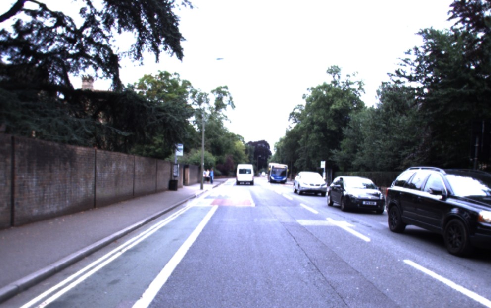
(a) reference image

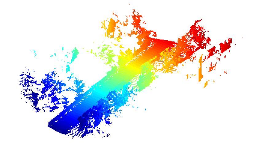
(b) 3D point cloud

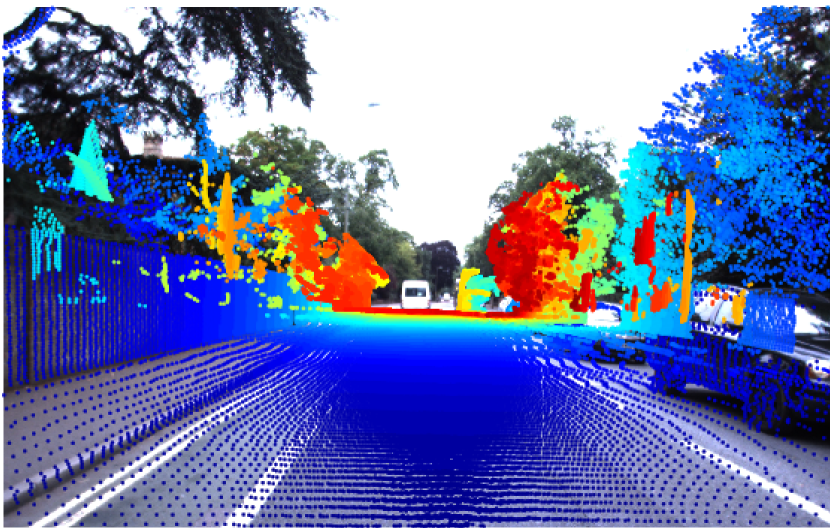
(c) projections

Fig. 14: An example of projecting the 3D point cloud into the reference image.

A.4 Perspective-n-Point and RANSAC

The set of 2D-3D correspondences $\hat{c}$ establishes one-to-one correspondences between 2D points in query image frame $\textbf{p}_{Q}^{(j)}$, and 3D points in the reference image frame $\textbf{P}^{(j)}$, for $j=1,2,\ldots,m$. The last step is to apply Perspective-n-Point solver (Gao et al., 2003) to compute the relative 6-DoF camera pose M between the query image and the reference image. For this purpose, two approaches are combined to solve the problem: the algebraic approach and the geometric approach. In the algebraic approach, we use Wu’s zero decomposition method to find a complete triangular decomposition of a practical configuration for the P3P problem (Gao et al., 2003). We can obtain up to 4 solutions for the pose using 3 points, and in the geometric approach, we choose the solution that results in smallest squared re-projection error for the 4th point (Gao et al., 2003),

$$\textbf{M}^{*}=\arg\min_{\textbf{M}}\sum_{\forall{i}}\|\textbf{p}_{Q}^{(i)}-\textbf{K}\textbf{M}\textbf{P}^{(i)}\|,\quad i\in\{1,2\ldots,m\}$$ (11)

where M is the sought word-to-camera transformation matrix, $\textbf{M}^{*}$ is its best estimate, K is the intrinsic matrix, $\textbf{p}_{Q}^{(i)}$ is the $i$-th feature point at the query image and $\textbf{P}^{(i)}$ is its corresponding 3D coordinate.

In reality, the set of 2D-3D correspondences $\hat{c}$ can be corrupted by outliers, so it is common to use a robust estimator together with PnP slovers. RANSAC (Fischler and Bolles, 1981) estimator is a popular choice, and in our work we use a generalization of the RANSAC estimator, MLESAC (Torr and Zisserman, 2000). MLESAC adopts the same sampling strategy as RANSAC to generate putative solutions, but chooses the solutions by maximizing the likelihood rather than just the number of inliers.

Finally, the 6-DoF camera pose can be obtained by means of the decomposition of $\textbf{M}^{*}$ via (6).

Appendix B Direct photometric-based camera pose estimation

This appendix explains the details of the three stages of the direct photometric-based camera pose estimation, namely, generation of synthetic views, direct photometric matching and coarse-to-fine search.

B.1 Generation of synthetic views

The reference 3D point cloud $P_{R}$ does not have any color or intensity information, but this information can be retrieved from the reference image as follows. Firstly, we project 3D point clouds $P_{R}=[\textbf{P}_{R}^{(1)},\textbf{P}_{R}^{(2)},\ldots,\textbf{P}_{R}^{(m)}]$ onto the reference image plane using (5) and get a set of 2D projections, $p=[\textbf{p}^{(1)},\textbf{p}^{(2)},\ldots,\textbf{p}^{(m)}]$. This process is the same as Fig. 14(c). Secondly, we use cubic interpolation to compute the intensity values for each 2D projection and assign the intensity values to the 3D point cloud as:

$$I(\textbf{P}_{R}^{(i)})\leftarrow f(\textbf{p}_{R}^{(i)},I_{R}),\quad I_{R}\in\mathbb{R}^{2}$$ (12)

where $I_{R}$ is the reference image, $\textbf{p}^{(i)}$ is the $i$-th 2D projection, $I(\textbf{P}_{R}^{(i)})$ is the intensity value of the 3D point $\textbf{P}_{R}^{(i)}$, and $f$ is the cubic interpolation function. As a result, we assign intensity (or color) information to the 3D point cloud $P_{R}$.

Synthetic views can now be rendered by projecting the colored 3D point cloud using a transformation matrix M using (5), and the intensities of the synthetic view $I_{S}$ can be obtained as:

$$I_{S}(\textbf{K}\textbf{M}\textbf{P}_{R}^{(i)})\leftarrow I(\textbf{P}_{R}^{(i)}),$$ (13)

where $I(\textbf{P}_{R}^{(i)})$ is the intensity value of the $i$-th 3D point $\textbf{P}_{R}^{(i)}$, K is the intrinsic matrix, M is the world-to-synthetic-view transformation, and $I_{S}(\textbf{K}\textbf{M}\textbf{P}_{R}^{(i)})$ is the intensity value of the projection of the 3D point $\textbf{P}_{R}^{(i)}$ at the synthetic frame. Synthetic views are quickly rendered by the standard computer graphics procedure of surface splatting (Zwicker et al., 2001).

B.2 Direct photometric matching

The direct photometric-based approach (Tykkälä et al., 2013) is defined as a direct minimization of the cost function at the space of 6D camera pose, and in the cost function it compares the pixel intensities of the query image $I_{Q}$ and rendered synthetic view $I_{S}$ from the colored 3D point cloud (Tykkälä et al., 2013). The task is to find the best relative camera transform $\textbf{M}^{*}$ that minimizes the photometric-error between query image $I_{Q}$ and synthetic image $I_{S}$:

$$\textbf{M}^{*}=\arg\min_{\textbf{M}}\text{RSE}(I_{Q},I_{S}),$$ (14)

where,

$$\text{RSE}(I_{Q},I_{S})=\dfrac{1}{\mu}\sum_{(u,v)\in{I_{S}}}(I_{Q}(u,v)-I_{S}(u,v))^{2}$$ (15)

In (15) the synthetic view $I_{S}$ is generated by (13), and $\mu$ is the number of pixels in $I_{S}$.

To improve the robustness of the matching process, we smooth the query image $I_{S}$ by using a Gaussian filter and then we use the smoothed version of query image in the image matching process. Moreover, we use M-estimator to improve the matching process, since the M-estimator can be used for managing outliers when the residual vector is of sufficient length for statistical purpose (Huber, 2011). The main idea is to generate small weights for residual elements that are classified as outliers by analyzing the distribution of residual values. Inliers always have small residual values whereas outliers may have any error value. In our work, we use the median filter to find the median value among the residuals, $\mbox{RSE}(I_{Q},I_{S})$, then give zero weights to all the residual values that are greater than the median value, and give normalized weights to the the remain residuals.

With the M-estimator, we can rewrite (15) as the average of the weighted sum-of-square difference:

$$\mbox{RSE}(I_{Q},I_{S})=\dfrac{1}{\lambda}\sum_{\forall{(u,v)}}{(E(u,v))}^{2}w(u,v)$$ (16)

where we apply the weights to the residual vector and compute the average of the weighted sum-of-square difference, and $\lambda$ is the number of nonzero weights. $E(u,v)$ and $w(u,v)$ are defined in (17) and (18) as follows:

$$E(u,v)=(I_{Q}(u,v)-I_{S}(u,v))^{2},(u,v)\in{I_{S}}$$ (17)

where $I_{Q}$ is the query image, $I_{S}$ is the synthetic image, and $E$ is the difference between the two images.

$$w(u,v)=\begin{cases}0,&\text{if }E(u,v)>\theta\\ 1,&\text{otherwise}\end{cases}$$ (18)

where $\theta$ is the median value of of $E(u,v)$ and $(u,v)\in{I_{S}}$.

B.3 Coarse-to-fine grid search

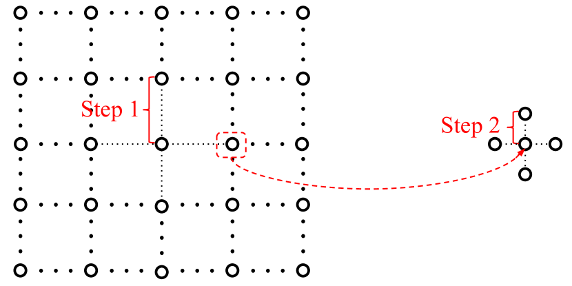
Fig. 15: Coarse-to-fine grid search for translation. Grids are placed along x (toward to the right of the camera) and y (toward to the front of the camera) axis. Start to search the minimum with a big step (step 1) in a grid manner, then follow a smaller step (step 2) search in a grid manner again at the previous minimum location.

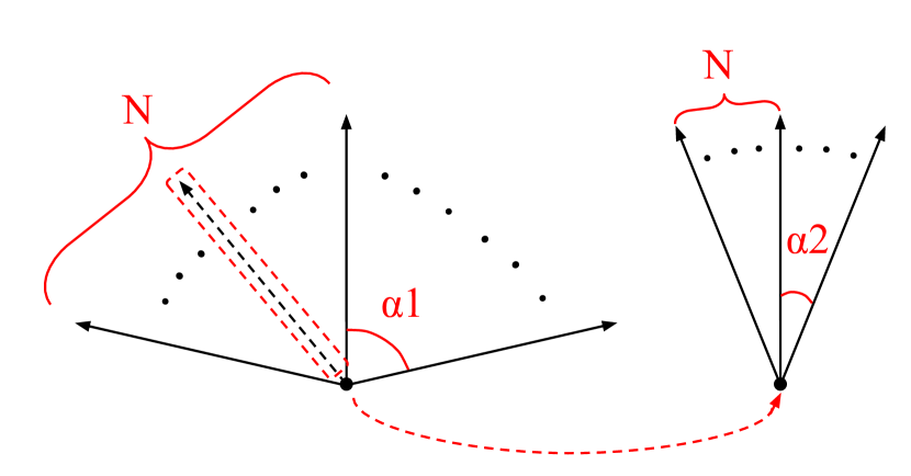
Fig. 16: Coarse-to-fine grid search for orientation. For the selected axis (z axis, toward up of the camera), start to search the minimum with a big orientation search range $2\times\alpha 1$ with $2\times N-1$ steps, then follow a smaller orientation search range $2\times\alpha 2$ with $2\times N-1$ steps in a grid manner again at the previous minimum orientation.

we use a two-step coarse-to-fine grid search to solve for the matrix $\textbf{M}^{*}$ in (14), The coarse-to-fine grid search concatenates search with a coarse step for the local minimum with a subsequent search with at a finer step at the location of the previous minimum location. We apply the coarse-to-fine search firstly to the translation, and based on the previous minimum, we then apply it to the orientation. The process of the coarse-to-fine grid search is illustrated in Fig. 15 and Fig. 16.

Firstly, we defined a 2D search grid along x (towards the right of the camera) and z (toward the front of the camera) axis directions, and the origin is in the middle of the 2D search grid. We start to search the minimum with a big step (step 1) in a grid manner, then follow a smaller step (step 2) search in a grid manner again at the previous minimum location. Fig. 15 illustrated the coarse-to-fine search for translation.

Secondly, based on the previous minimum location, we further apply the coarse-to-fine grid search for orientation. We could search the optimal orientations along one more multiple axis. For our experiments, we search the optimal orientations along the z axis (toward up direction of the car). As shown in Fig. 16, We start to search the minimum with a big orientation search range $2\times\alpha 1$ with $2\times N-1$ steps, then follow a smaller orientation search range $2\times\alpha 2$ with $2\times N-1$ steps in a grid manner again at the previous minimum orientation.

References

- Alahi et al. (2012) Alahi, A., Ortiz, R., Vandergheynst, P., 2012. Freak: Fast retina keypoint, in: Computer vision and pattern recognition (CVPR), 2012 IEEE conference on, Ieee. pp. 510–517.
- Ambai and Yoshida (2011) Ambai, M., Yoshida, Y., 2011. Card: Compact and real-time descriptors, in: Computer Vision (ICCV), 2011 IEEE International Conference on, IEEE. pp. 97–104.
- Bay et al. (2006) Bay, H., Tuytelaars, T., Van Gool, L., 2006. Surf: Speeded up robust features. Computer vision–ECCV 2006 , 404–417.
- Belongie et al. (2001) Belongie, S., Malik, J., Puzicha, J., 2001. Shape context: A new descriptor for shape matching and object recognition, in: Advances in neural information processing systems, pp. 831–837.
- Calonder et al. (2010) Calonder, M., Lepetit, V., Strecha, C., Fua, P., 2010. Brief: Binary robust independent elementary features. Computer Vision–ECCV 2010 , 778–792.
- Castellanos and Tardos (2012) Castellanos, J.A., Tardos, J.D., 2012. Mobile robot localization and map building: A multisensor fusion approach. Springer Science & Business Media.
- Csurka et al. (2004) Csurka, G., Dance, C., Fan, L., Willamowski, J., Bray, C., 2004. Visual categorization with bags of keypoints, in: Workshop on statistical learning in computer vision, ECCV, Prague. pp. 1–2.
- Dalal and Triggs (2005) Dalal, N., Triggs, B., 2005. Histograms of oriented gradients for human detection, in: Computer Vision and Pattern Recognition, 2005. CVPR 2005. IEEE Computer Society Conference on, IEEE. pp. 886–893.
- Fischler and Bolles (1981) Fischler, M.A., Bolles, R.C., 1981. Random sample consensus: a paradigm for model fitting with applications to image analysis and automated cartography. Communications of the ACM 24, 381–395.
- Friedman et al. (1977) Friedman, J.H., Bentley, J.L., Finkel, R.A., 1977. An algorithm for finding best matches in logarithmic expected time. ACM Transactions on Mathematical Software (TOMS) 3, 209–226.
- Froba and Ernst (2004) Froba, B., Ernst, A., 2004. Face detection with the modified census transform, in: Automatic Face and Gesture Recognition, 2004. Proceedings. Sixth IEEE International Conference on, IEEE. pp. 91–96.
- Gao et al. (2003) Gao, X.S., Hou, X.R., Tang, J., Cheng, H.F., 2003. Complete solution classification for the perspective-three-point problem. IEEE transactions on pattern analysis and machine intelligence 25, 930–943.
- Geiger et al. (2012) Geiger, A., Lenz, P., Urtasun, R., 2012. Are we ready for autonomous driving? the kitti vision benchmark suite, in: Conference on Computer Vision and Pattern Recognition (CVPR).
- Guo et al. (2010) Guo, Z., Zhang, L., Zhang, D., 2010. Rotation invariant texture classification using lbp variance (lbpv) with global matching. Pattern recognition 43, 706–719.
- Huber (2011) Huber, P.J., 2011. Robust statistics. Springer.
- Irschara et al. (2009) Irschara, A., Zach, C., Frahm, J.M., Bischof, H., 2009. From structure-from-motion point clouds to fast location recognition, in: 2009 IEEE Conference on Computer Vision and Pattern Recognition, pp. 2599–2606.
- Iscen et al. (2017) Iscen, A., Tolias, G., Avrithis, Y., Furon, T., Chum, O., 2017. Efficient diffusion on region manifolds: Recovering small objects with compact CNN representations, in: CVPR.
- Kadir and Brady (2001) Kadir, T., Brady, M., 2001. Saliency, scale and image description. International Journal of Computer Vision 45, 83–105.
- Kim et al. (2014) Kim, H., Lee, D., Oh, T., Lee, S.W., Choe, Y., Myung, H., 2014. Feature-based 6-dof camera localization using prior point cloud and images, in: Robot Intelligence Technology and Applications 2. Springer, pp. 3–11.
- Klaser et al. (2008) Klaser, A., Marszałek, M., Schmid, C., 2008. A spatio-temporal descriptor based on 3d-gradients, in: BMVC 2008-19th British Machine Vision Conference, British Machine Vision Association. pp. 275–1.
- Leutenegger et al. (2011) Leutenegger, S., Chli, M., Siegwart, R.Y., 2011. Brisk: Binary robust invariant scalable keypoints, in: Computer Vision (ICCV), 2011 IEEE International Conference on, IEEE. pp. 2548–2555.
- Lienhart and Maydt (2002) Lienhart, R., Maydt, J., 2002. An extended set of haar-like features for rapid object detection, in: Image Processing. 2002. Proceedings. 2002 International Conference on, IEEE.
- Linegar et al. (2016) Linegar, C., Churchill, W., Newman, P., 2016. Made to measure: Bespoke landmarks for 24-hour, all-weather localisation with a camera, in: Robotics and Automation (ICRA), 2016 IEEE International Conference on, IEEE. pp. 787–794.
- Lowe (1999) Lowe, D.G., 1999. Object recognition from local scale-invariant features, in: Computer vision, 1999. The proceedings of the seventh IEEE international conference on, Ieee. pp. 1150–1157.
- Lowe (2004) Lowe, D.G., 2004. Distinctive image features from scale-invariant keypoints. International journal of computer vision 60, 91–110.
- Maddern et al. (2017) Maddern, W., Pascoe, G., Linegar, C., Newman, P., 2017. 1 Year, 1000km: The Oxford RobotCar Dataset. The International Journal of Robotics Research (IJRR) 36, 3–15.
- Mani and rivazhagan (2013) Mani, V., rivazhagan, D., 2013. Survey of medical image registration. Journal of Biomedical Engineering and Technology 1, 8–25.
- Markley et al. (2007) Markley, F.L., Cheng, Y., Crassidis, J.L., Oshman, Y., 2007. Averaging quaternions. Journal of Guidance Control and Dynamics 30, 1193.
- Matas et al. (2004) Matas, J., Chum, O., Urban, M., Pajdla, T., 2004. Robust wide-baseline stereo from maximally stable extremal regions. Image and vision computing 22, 761–767.
- McDaid et al. (2011) McDaid, A.F., Greene, D., Hurley, N., 2011. Normalized mutual information to evaluate overlapping community finding algorithms. arXiv preprint arXiv:1110.2515 .
- Mikolajczyk and Schmid (2004) Mikolajczyk, K., Schmid, C., 2004. Scale & affine invariant interest point detectors. International journal of computer vision 60, 63–86.
- Mishkin et al. (2015) Mishkin, D., Matas, J., Perdoch, M., 2015. Mods: Fast and robust method for two-view matching. Computer Vision and Image Understanding 141, 81–93.
- Miura et al. (2015) Miura, S., Hsu, L.T., Chen, F., Kamijo, S., 2015. Gps error correction with pseudorange evaluation using three-dimensional maps. IEEE Transactions on Intelligent Transportation Systems 16, 3104–3115.
- Mori et al. (2004) Mori, G., Ren, X., Efros, A.A., Malik, J., 2004. Recovering human body configurations: Combining segmentation and recognition, in: Computer Vision and Pattern Recognition, 2004. CVPR 2004. Proceedings of the 2004 IEEE Computer Society Conference on, IEEE. pp. II–II.
- Muja and Lowe (2009) Muja, M., Lowe, D.G., 2009. Fast approximate nearest neighbors with automatic algorithm configuration. VISAPP (1) 2, 2.
- Mur-Artal et al. (2015) Mur-Artal, R., Montiel, J.M.M., Tardos, J.D., 2015. Orb-slam: a versatile and accurate monocular slam system. IEEE Transactions on Robotics 31, 1147–1163.
- Newcombe et al. (2011a) Newcombe, R.A., Izadi, S., Hilliges, O., Molyneaux, D., Kim, D., Davison, A.J., Kohi, P., Shotton, J., Hodges, S., Fitzgibbon, A., 2011a. Kinectfusion: Real-time dense surface mapping and tracking, in: Mixed and augmented reality (ISMAR), 2011 10th IEEE international symposium on, IEEE. pp. 127–136.
- Newcombe et al. (2011b) Newcombe, R.A., Lovegrove, S.J., Davison, A.J., 2011b. Dtam: Dense tracking and mapping in real-time, in: Computer Vision (ICCV), 2011 IEEE International Conference on, IEEE. pp. 2320–2327.
- Ohta and Tamura (2014) Ohta, Y., Tamura, H., 2014. Mixed reality: merging real and virtual worlds. Springer Publishing Company, Incorporated.
- Ojala et al. (2002) Ojala, T., Pietikainen, M., Maenpaa, T., 2002. Multiresolution gray-scale and rotation invariant texture classification with local binary patterns. IEEE Transactions on pattern analysis and machine intelligence 24, 971–987.
- Pascoe et al. (2017) Pascoe, G., Maddern, W., Tanner, M., Pinies, P., Newman, P., 2017. NID-SLAM: Robust monocular SLAM using normalised information distance, in: Proceedings of the IEEE Conference on Computer Vision and Pattern Recognition (CVPR), Honolulu, HI.
- Philbin et al. (2007) Philbin, J., Chum, O., Isard, M., Sivic, J., Zisserman, A., 2007. Object retrieval with large vocabularies and fast spatial matching, in: Computer Vision and Pattern Recognition, 2007. CVPR’07. IEEE Conference on, IEEE. pp. 1–8.
- Radenović et al. (2016) Radenović, F., Tolias, G., Chum, O., 2016. CNN image retrieval learns from BoW: Unsupervised fine-tuning with hard examples, in: ECCV.
- Rosten and Drummond (2006) Rosten, E., Drummond, T., 2006. Machine learning for high-speed corner detection. Computer vision–ECCV 2006 , 430–443.
- Rublee et al. (2011) Rublee, E., Rabaud, V., Konolige, K., Bradski, G., 2011. Orb: An efficient alternative to sift or surf, in: Computer Vision (ICCV), 2011 IEEE International Conference on, IEEE. pp. 2564–2571.
- Sattler et al. (2016) Sattler, T., Havlena, M., Schindler, K., Pollefeys, M., 2016. Large-scale location recognition and the geometric burstiness problem, in: The IEEE Conference on Computer Vision and Pattern Recognition (CVPR).
- Scovanner et al. (2007) Scovanner, P., Ali, S., Shah, M., 2007. A 3-dimensional sift descriptor and its application to action recognition, in: Proceedings of the 15th ACM international conference on Multimedia, ACM. pp. 357–360.
- Song et al. (2016) Song, Y., Chen, X., Wang, X., Zhang, Y., Li, J., 2016. 6-dof image localization from massive geo-tagged reference images. IEEE Transactions on Multimedia 18, 1542–1554.
- Strecha et al. (2012) Strecha, C., Bronstein, A., Bronstein, M., Fua, P., 2012. Ldahash: Improved matching with smaller descriptors. IEEE Transactions on Pattern Analysis and Machine Intelligence 34, 66–78.
- Taylor (2016) Taylor, A.G., 2016. Develop Microsoft HoloLens Apps Now. 1st ed., Apress, Berkely, CA, USA.
- Tola et al. (2010) Tola, E., Lepetit, V., Fua, P., 2010. Daisy: An efficient dense descriptor applied to wide-baseline stereo. IEEE transactions on pattern analysis and machine intelligence 32, 815–830.
- Torr and Zisserman (2000) Torr, P.H., Zisserman, A., 2000. Mlesac: A new robust estimator with application to estimating image geometry. Computer Vision and Image Understanding 78, 138–156.
- Tuytelaars et al. (2008) Tuytelaars, T., Mikolajczyk, K., et al., 2008. Local invariant feature detectors: a survey. Foundations and trends® in computer graphics and vision 3, 177–280.
- Tuytelaars and Van Gool (2004) Tuytelaars, T., Van Gool, L., 2004. Matching widely separated views based on affine invariant regions. International journal of computer vision 59, 61–85.
- Tuytelaars and Van Gool (2000) Tuytelaars, T., Van Gool, L.J., 2000. Wide baseline stereo matching based on local, affinely invariant regions., in: BMVC.
- Tykkälä et al. (2013) Tykkälä, T., Comport, A.I., Kämäräinen, J.K., 2013. Photorealistic 3d mapping of indoors by rgb-d scanning process, in: Intelligent Robots and Systems (IROS), 2013 IEEE/RSJ International Conference on, IEEE. pp. 1050–1055.
- Zahn and Roskies (1972) Zahn, C.T., Roskies, R.Z., 1972. Fourier descriptors for plane closed curves. IEEE Transactions on computers 100, 269–281.
- Zhao and Pietikainen (2007) Zhao, G., Pietikainen, M., 2007. Dynamic texture recognition using local binary patterns with an application to facial expressions. IEEE transactions on pattern analysis and machine intelligence 29.
- Zwicker et al. (2001) Zwicker, M., Pfister, H., van Baar, J., Gross, M., 2001. Surface splatting, in: ACM SIGGRAPH.