IEEE Copyright Notice

Federico Terraneo1, Alberto Leva1, Silvano Seva1, Martina Maggio2, Alessandro Vittorio Papadopoulos2 1Politecnico di Milano, Milano, Italy 2Lund University, Lund, Sweden

Copyright (c) 2015 IEEE. Personal use of this material is permitted. Permission from IEEE must be obtained for all other uses, in any current or future media, including reprinting/republishing this material for advertising or promotional purposes, creating new collective works, for resale or redistribution to servers or lists, or reuse of any copyrighted component of this work in other works.

F. Terraneo, A. Leva, S. Seva, M. Maggio, A. V. Papadopoulos, ”Reverse Flooding: exploiting radio interference for efficient propagation delay compensation in WSN clock synchronization” IEEE Real-Time Systems Symposium (RTSS), San Antonio, Texas, December 2015.

https://doi.org/10.1109/RTSS.2015.24

Reverse Flooding: exploiting radio interference for efficient propagation delay compensation in WSN clock synchronization

Federico Terraneo1, Alberto Leva1, Silvano Seva1, Martina Maggio2, Alessandro Vittorio Papadopoulos2 1Politecnico di Milano, Milano, Italy 2Lund University, Lund, Sweden

Abstract

Clock synchronization is a necessary component in modern distributed systems, especially Wirless Sensor Networks. Despite the great effort and the numerous improvements, the existing synchronization schemes do not yet address the cancellation of propagation delays. Up to a few years ago, this was not perceived as a problem, because the time-stamping precision was a more limiting factor for the accuracy achievable with a synchronization scheme. However, the recent introduction of efficient flooding schemes based on constructive interference has greatly improved the achievable accuracy, to the point where propagation delays can effectively become the main source of error.

In this paper, we propose a method to estimate and compensate for the network propagation delays. Our proposal does not require to maintain a spanning tree of the network, and exploits constructive interference even to transmit packets whose content are slightly different. To show the validity of the approach, we implemented the propagation delay estimator on top of the FLOPSYNC-2 synchronization scheme. Experimental results prove the feasibility of measuring propagation delays using off-the-shelf microcontrollers and radio transceivers, and show how the proposed solution allows to achieve sub-microsecond clock synchronization even for networks where propagation delays are significant.

I Introduction

Clock synchronization in distributed systems is a problem with a long history [16, 13]. Recently, the diffusion of WSNs has drawn more attention to specific variants of the problem. Indeed, there are many different clock synchronization problems, depending on the settings and the desired properties that a synchronization scheme should achieve. The following work is cast in the framework of multi-hop master-slave clock synchronization.

In the specific problem addressed in this paper, the network is composed by a certain number of slave nodes and a single master node. The slave nodes are organized in hops, around the master node, which is the only node belonging to Hop 0. The master node has a limited transmission range and directly reaches nodes belonging to Hop 1. In turn, nodes belonging to Hop 1 can re-broadcast the messages received from the master node and reach nodes that are farther away, not belonging to the master range. These nodes belong to Hop 2 and can receive master communications only due to the re-transmission of the nodes that directly receive the master node packets. The procedure can be repeated adding an arbitrarily large number of nodes and hops. The problem, in this case, is to synchronize the clocks of all the slave nodes to the clock of the master node, irregardless of the hop they belong to.

While there are quite a few solutions for the master-slave multi-hop synchronization problem [22, 14, 6, 1], none of them takes directly into account the propagation delay of the packets on the network. Historically, the propagation delay was not a big issue. The most limiting factor to what a synchronization scheme could achieve was the time-stamping precision. However, quoting from [26], “While [propagation delay] is not a problem if time-stamping precision is worse than about 1 $\mu$s, it starts to be a significant source of error at appreciably finer precisions”.

The recent introduction of flooding schemes based on constructive interference like Glossy [27], has changed the WSN synchronization scenario. Making the flooding mechanism insensitive to MAC-induced delays has in fact allowed to disseminate timing information with unprecedented precision. Moreover, skew compensation techniques have also advanced, allowing for sub-microsecond precision also in ultra-low power networks [1]. In these conditions, propagation delays become a problem to be addressed.

In this paper we present a delay compensation method that can be built on top of any asymmetric master-slave clock synchronization scheme based on constructive interference flooding. This paper makes the following contributions.

• It enhances a master-slave synchronization scheme, exploiting the proposed method to estimate and compensate for the propagation delay from the master node to any slave node in a WSN without the need for a spanning tree of the network.

• As a second methodological contribution, it presents a technique to allow the concurrent transmission of multiple packets having a different payload. The method is capable of exploiting the constructive interference despite the different payloads, resulting in an intelligible message for the intended recipient.

To show the applicability of the technique we implemented the proposed delay compensator on top of the FLOPSYNC-2 synchronization scheme [1], showing how the method improves time synchronization in a WSN where sensors are deployed within a radius that causes propagation delay to be the major source of error.

II Problem statement

Consider a multi-hop WSN with one master node and a certain number of slave nodes. Each node is equipped with a synchronization scheme based on a MAC-level flooding scheme like Glossy [27].

If we assume that nodes do not move, it is possible to define a flooding graph for the network. The flooding graph is a subgraph of the directed graph connecting all nodes of hop $h$ with all nodes of hop $h+1$ for each network hop. The edges missing in the flooding graph with respect to the complete one are due to distances. In fact, if a receiver node is not in the radio range of the transmitter one, the corresponding edge is removed from the flooding graph.

Figure 1: Flooding graph example with nodes’ radio ranges.

Figure 1 shows an example. The Hop 0 is composed by the master node, marked with the letter M. Nodes 1, 2 and 3 belongs to Hop 1, since they are in the radio range of the master node (depicted in the figure with a dotted circle centered on the master node). Nodes 4, 5 and 6 belong to Hop 2, since they are in the radio range of at least one of the nodes belonging to Hop 1. The remaining nodes, 7 and 8, belong to Hop 3 – their radio range is not shown to simplify the picture. Hop 3 illustrates also another characteristic of the network. Nodes belonging to a hop do not, in general, receive packets from all the nodes in the previous one. In the case of Hop 3, node 7 belongs to the radio range of node 4 (and would not receive any packet from node 5 and 6), node 8 belongs to the radio range of both node 5 and node 6 (but not of node 4) and node 9 receives packets only from node 6. As nodes belonging to a hop can receive packets from multiple nodes belonging to the previous one, in general the flooding graph is not a tree. This motivates the need to exploit the constructive interference between packets transmitted by nodes that are close to each other.

We would like each node to be able to reliably estimate the propagation delay from the master node to it. This is complicated by the fact that the flooding graph is not a tree and that nodes do not possess knowledge about its structure. In fact, with a spanning tree and knowledge about the tree structure, each node $i$ could estimate via round-trip delay measurements the propagation delay $\delta_{i\rightarrow p}$ from its sole predecessor $p$ and could simply ask to the predecessor the cumulated delay $\delta_{M\rightarrow p}$ from the master $M$ to $p$. Then the node $i$ would have an estimate of the delay from the master: $\delta_{M\rightarrow i}=\delta_{i\rightarrow p}+\delta_{M\rightarrow p}$. We propose a solution based on the same principles, that takes into account the nature of the graph and the constructive interference in the transmissions.

The main difficulties when dealing with the flooding graph and constructive interference are the following.

1. The node $i$ does not have a single predecessor $p$ but a set of predecessors $\mathcal{P}_{i}=\{p_{1},\dots,p_{n}\}$ and receives the flooded timing information by the entire set of predecessors; round-trip measurements in such a scenario need to take this into account.

2. When node $i$ queries nodes in $\mathcal{P}_{i}$ for their cumulated delay from the master node, they will simultaneously send back (potentially) different responses, that should be fused in a meaningful manner.

3. The node $i$ does not know which are the nodes that form the set $\mathcal{P}_{i}$. More in general nodes should query one another for round-trip times along the flooding graph, but none of them knows the structure of the graph. One of the major strength of interference-based flooding – not knowing which are the nodes that constructively interfere to provide timing information – turns here into a problem.

In Section III we describe how a node can estimate the propagation delay from its predecessor set $\mathcal{P}_{i}$ without knowing which nodes belong to it. In Section IV we propose an encoding method to fuse the different responses about the cumulated delay from the master node. Neither of these two require knowledge of the flooding graph. Section V describes a suitable Time Division Multiple Access (TDMA) method so that all the nodes of the network can perform the two tasks just mentioned. Section VI presents and discusses experimental results.

III Last-hop delay measurement

In this section we show how a node $i$ can measure the propagation delay from its predecessor set $\mathcal{P}_{i}$ (in contrast to the propagation delay from a single node). The first step is to define which nodes belong to the predecessor set $\mathcal{P}_{i}$. In so doing, we ensure that the node does not need any information about the flooding graph.

Figure 2: Example of flooding and the capture effect.

Consider node 4 in the example of Figure 1 (to help the reader, node 4, its predecessor set and the master node are shown in Figure 2). The node is placed in the radio range of nodes 1, 2 and 3, but the distances between these nodes and node 4 are different – node 1 and 2 are closer to the node while the distance from node 3 is larger.

During flooding, node 4 receives the packets sent concurrently by nodes node 1 and 2 thanks to the constructive interference. However, since node 3 is farther, its signal is received as weaker than those of nodes 1 and 2. Due to capture effects [5], the packet sent from node 3 is shadowed by the stronger signals of nodes 1 and 2. Indeed, flooding schemes like Glossy require all nodes to transmit with the same power [27]. This ensures that nodes that are more distant, thus having a higher propagation delay, have a weaker signal.

A node $p$ belonging to the previous hop is either at a comparable distance with the closest nodes, having enough power to interfere constructively, or its transmission is shadowed by capture effects. In case the node is at a comparable distance with the closest ones, its cumulative propagation delay from the master $\delta_{M\rightarrow p}$ is also comparable to the one of the closest nodes. With respect to Figure 2, $\delta_{M\rightarrow 1}$ and $\delta_{M\rightarrow 2}$ are comparable, while $\delta_{M\rightarrow 3}$ could be different, but its transmission is not processed by node 4. This property allows us to define the predecessor set $\mathcal{P}$ of node $i$ as the set of the closest nodes in the previous hop that are received with a comparable power. In the example, $\mathcal{P}_{4}=\{1,2\}$.

Once the predecessor set $\mathcal{P}_{i}$ is defined, node $i$ needs to measure the last-hop propagation delay. To do so without knowing the flooding graph, the key idea is to replicate in a round-trip measurement the same conditions of concurrent transmission that occur during flooding. To achieve this, we reserve a short time window after flooding, where the MAC protocol is still disabled and the radio channel is still clear from access contention.

Referring again to the example in Figure 2, within its time window, node 4 can initiate the measurement by sending a packet with its hop number minus one (in the example, 1). The difference with respect to standard round-trip estimation is the packet content. While in standard round-trip estimation the request packet contains the unique id of a node, in this case the packet contains the hop that should respond to the message. This is exemplified in the top part of Figure 3.

Figure 3: Round-trip measurement initiated by node 4 – request (top) and response (bottom).

Due to the radio range of the node and the definition of hops, the packet sent by node $i$ can only be received by nodes belonging to the previous, same and subsequent hop. A node $m$ that receives the packet checks that the content matches its own hop number. In case it does not, the node simply ignores the request. Otherwise, $m$ waits for a fixed time $\tau_{w}$ and then replies with another packet. As we have assumed that all nodes transmit at the same power, the radio ranges are symmetric, and the packet sent by node 4 is received by nodes 1, 2, 3, 5 and 7. Node 5 and 7 ignore the packet, while the others process it. Notice that also node 3 receives the request packet. The distance of node 3 does not make any difference in this case, since a single packet is being sent, contrary to multiple interfering ones. After a fixed time, nodes 1, 2 and 3 reply with an answer packet to node 4, replicating the same concurrent transmission condition of flooding – in this case, the response packet sent by node 3 will again be shadowed by the stronger signal of nodes 1 and 2 – as shown in the bottom part of Figure 3.

The $i$-th node can measure the time difference between its packet transmission and the reception and, knowing $\tau_{w}$, can estimate the propagation delay from the nodes that belong to $\mathcal{P}_{i}$, without knowing them.

IV Cumulated delay estimation

Once the node $i$ has an estimate of the last-hop delay, it needs to obtain an estimate of the sum of all the propagation delays for each additional hop that separates it from the master. We solve the problem recursively, querying nodes in the previous hop for their cumulated delay from the master.

Although the capture effects ensure that constructive interference occurs only between nodes at a comparable distance from the receiver, one should also take into account noise in round-trip measurements and small distance differences. These may cause the nodes in a predecessor set to have similar but not equal delay measurements from the master. For example, node 1 and 2 in Figure 2 may have similar but not equal cumulated delay values, $\delta_{M\rightarrow 1}=\delta_{M\rightarrow 2}+\varepsilon$ for small values of $\varepsilon$. While this is not a problem for the estimate of the last-hop delay, it becomes a problem for the cumulated delay. Since the nodes do not have knowledge of the flooding graph, they cannot simply query one specific node. In the example, if node 4 knew its predecessors, it could simply ask the cumulated delay to 1 and 2 separately, and then average the response. However, node 1 and 2 will transmit their responses concurrently.

To date, WSN interference was studied [3, 17, 23] and constructive interference used to transmit the same packet. We propose a method to fuse packets with different payloads and transmitted simultaneously from multiple sources.

To better understand what happens when different packets are received concurrently, it is necessary to briefly discuss the operation of an IEEE 802.15.4 radio, which is the most common standard for WSN. A packet is composed of a 4-byte preamble, used for the receiver to lock on the incoming data, followed by a one-byte start frame delimiter that marks the packet beginning. The following byte indicates the packet length. The payload follows, and finally a two-byte Cyclic Redundancy Check (CRC) terminates the packet. Data is grouped in 4-bit nibbles, and for each nibble a sequence of 32 bit from a look-up table is sent over the radio. This introduces redundancy in the transmitted data, improving reception in adverse conditions. The receiver, at each 32 decoded bits, attempts to find which of the 16 possible sequences best matches the received signal, and outputs the corresponding nibble.

The minimum transmission unit is one nibble, and when packets with different payloads are sent concurrently, every nibble that has the same value in all packets interferes constructively. On the contrary, nibbles that have different values interfere destructively, resulting in unpredictable nibbles being received.

IV-A Concurrent transmission through bar graph encoding

We propose to utilize an ad hoc encoding, which we denote as bar graph encoding, that results in intelligible packets even when some nibbles interfere destructively.

To better explain the concept behind the bar graph encoding, assume to have an 8-bytes-long packet payload and to encode a number, bounded in the range between 0 and 16 as the number of consecutive 0xf nibbles starting from the beginning of the packet, leaving all other nibbles as 0x0. The number 0 would be encoded with a packet full of 0x0, the number 16 with a packet full of 0xf and, for example, the number 5 as ff ff f0 00 00 00 00 00. When sending two different numbers, for example 5 and 8, the two packets

ff ff f0 00 00 00 00 00
ff ff ff ff 00 00 00 00

will be transmitted, and the generic received packet will look like ff ff fX XX 00 00 00 00, with X being an unpredictable value. This encoding allows us to concurrently transmit different values, that the radio channel itself merges. In principle, the received unpredictable values could differ from 0x0 and 0xf, thus simplifying the estimate of the maximum and minimum index in the packet of the values sent concurrently. However, experimental results have shown that with high likelihood the unpredictable nibbles are a random pattern of either 0x0 or 0xf, while different values occur with a significantly lower probability.

In our proposal, the nodes send the cumulated delay using the bar graph encoding. Since the differences between the values sent by different nodes are small, we also assume that any possible value between the bounds of the sent one is acceptable. In the example above, the packet decoding would be successful if any value between 5 and 8 was returned.

With bar graph encoding, packets need to be sent without a CRC, otherwise the failed CRC due to nibble errors would result in the packet being discarded. Although the 802.15.4 standard prescribes a CRC at the end of each packet, radio transceivers such as the CC2520 have an option to disable its transmission. Packet decoding and validation is implemented by identifying the boundary from the left where two consecutive nibbles are different from 0xf, and the boundary from the right where two consecutive nibbles are different from 0x0. If the difference between the two boundaries is greater than a threshold, the packet is considered invalid and discarded. Otherwise, the average value between the two boundaries is considered as the transmitted number from the predecessor set. Notice that this decoding algorithm is robust to non-consecutive nibble errors anywhere within the payload. This favors correct reception also in adverse conditions, such as concurrent transmission of long packets. The full C++ implementation of the decoding algorithm used in the experimental evaluation is shown in Listing 1.

⬇

1pair<int,bool> decode(unsigned char *packet, int len)

2{

3 int pktLenNibble = 2*len;

4 int fromLeft = pktLenNibble - 1;

5 bool twoInaRow = false;

6 for(int i = 0; i < pktLenNibble; i++)

7 {

8 unsigned char mask = (i & 1) ? 0x0f : 0xf0;

9

10 if((packet[i/2] & mask) != mask)

11 {

12 if(twoInaRow)

13 {

14 fromLeft = i - 2;

15 twoInaRow = false;

16 break;

17 } else twoInaRow = true;

18 } else twoInaRow = false;

19 }

20 if(twoInaRow) fromLeft--;

21

22 int fromRight = 0;

23 twoInaRow = false;

24 for(int i = pktLenNibble - 1; i >= 0; i--)

25 {

26 unsigned char mask = (i & 1) ? 0x0f : 0xf0;

27 if((packet[i/2] & mask) != 0x00)

28 {

29 if(twoInaRow)

30 {

31 fromRight = i + 2;

32 twoInaRow = false;

33 break;

34 } else twoInaRow = true;

35 } else twoInaRow = false;

36 }

37 if(twoInaRow) fromRight++;

38

39 // If the destructive interference part of the packet

40 // is too large, discard the packet by returning false

41 const int threshold = 6;

42 if(fromRight - fromLeft > threshold)

43 return make_pair(0,false);

44

45 return make_pair((fromLeft + fromRight + 1) / 2,true);

46}

Listing 1: Bar graph encoding decoder algorithm.

802.15.4 packets have a maximum length of 127 bytes, thus the proposed technique permits the transmission of a number in the range $[0,254]$. Assuming that the timestamping resolution is $42\,$ns, as in the experimental results section, this allows us to handle propagation delays of up to $10.58\,\mu$s. In turn, we can synchronize nodes in a range of about $3\,$km from the master with the maximum precision allowed by our timestamping resolution. To handle larger distances, it is possible to lower the propagation delay resolution. As an extreme example, with a resolution of $1\,\mu$s, the range would extend to about $75\,$km.

The request sent by a node $i$ (4 in the example) to its predecessor set $\mathcal{P}_{i}$ (in the example $\mathcal{P}_{4}=\{1,2\}$) for the cumulated delay from the master, can be made implicit in the round-trip request packet described in Section III. The answer can be piggybacked to the round-trip answer packet, resulting in both round-trip estimation and cumulated delay communication with a single packet exchange.

V The complete scheme

This section describes how the last-hop delay measurement and the cumulated delay reception are composed to properly estimate the delay from the master. We assume for the moment that a network of $n$ nodes is already formed, and that each node has a unique id and knows its hop number, which is true if a flooding scheme like Glossy [27] is used.

Figure 4: Overall timeline for the proposed delay measurement scheme.

It is possible to reserve a short time interval after each flooding, to be used for propagation delay estimation. During this time interval, the MAC protocol used by the nodes in ordinary operations needs to be disabled as done during flooding. The interval is composed of $s$ time slots, with $1\leq s\leq n$. During these time slots, using a TDMA scheme, each node can estimate its propagation delay from the nodes in the previous hop, as explained in Section III. Since $n$ is known and each node knows its id, a simple round-robin scheme can be used for the TDMA. This means that all the nodes periodically estimate their propagation delay from the previous hop every $\lceil n/s\rceil$ synchronization periods. The parameter $s$ allows the scheme to trade off the radio bandwidth usage (and thus power consumption) for the speed at which a node becomes aware of propagation delay changes and, as will be shown in the following, the time required for network formation.

The overall operation of the scheme for one of the TDMA slots is summarised in Figure 4. During each of the $k$ time slots a single node (hereinafter, $i$, as the initiator), belonging to hop $h$, can send a propagation delay request packet. This packet is sent in broadcast, and the node timestamps its local Start Frame Delimiter (SFD) occurring at $\tau_{i,\texttt{start}}$. The request has a two-byte payload. The first byte is a packet type field identifying it as a round-trip request, and the second byte is $h-1$. The nodes whose hop number is not $h-1$ ignore the packet.

The nodes in the predecessor set $\mathcal{P}_{i}$ act collectively as the predecessor $p$, thanks to constructive interference. The predecessor, upon getting the request, waits for a fixed retransmission delay $\tau_{w}$, known network-wide and used to account for the transceiver turnaround and the duration of the request packet, as well as to absorb any software-induced jitter. The predecessor sends its response packet, and the initiator $i$ timestamps the corresponding SFD (occurring at $\tau_{i,\texttt{end}}$). The response packet contains the predecessor’s cumulated delay $\delta_{M\rightarrow p}$, encoded in bar graph form. Note that there is no need to include a timestamp neither in the request nor in the response packets.

Node $i$ then takes the difference $\tau_{i,\texttt{end}}-\tau_{i,\texttt{start}}$, and subtracts the retransmission delay $\tau_{w}$, the duration of a four-byte preamble plus SFD, and an additional short time – a transceiver-specific parameter that can be easily measured in a laboratory setting – for the lag in the SFD detection. The result, as evidenced in Figure 4, is twice the propagation delay from the predecessor, whence the measurement of $\delta_{p\rightarrow i}$. Finally, by inspecting the response packet content, the initiator obtains the value of $\delta_{M\rightarrow p}$, therefore completing the estimate of the full delay from the master $\delta_{M\rightarrow i}$.

This process is prone to three main source of errors:

• possible variations in the propagation delay due for example to scattering caused by moving obstacles;

• jitter in the SFD lag entity;

• quantization in turning the round-trip time in a measurement counted in clock ticks.

The first error source is highly environment-dependent, and hardly any general consideration can be made on it. That is why in the following we show both indoor and outdoor experiments, testifying that the caused errors are within a tolerable range. For the latter two causes, the SFD detection lag has a small variance [26], so the resulting error is comparable with one tick of the counting clock. Since we used off-the-shelf components, we can conjecture that our finding is general.

Using the estimate of the cumulated delay $\delta_{M\rightarrow i}$ node $i$ can compute a compensation term $c_{i}(k)$ at time instant $k$ ($k$ counts the number of times the node has transmitted a propagation delay request packet). The compensation term $c_{i}(k)$ is then applied at the clock of node $i$ to enhance synchronization.

First, $c_{i}(k)$ is subjected to a sanity check to eliminate evident outliers, verifying for example that the round-trip delay from the last hop is not outside the radio range. Despite this sanity check, two other issues should be taken into account. First, it is important to reduce as much as possible the jitter of the compensation term caused by measurement errors and moving obstacles. Second, synchronization schemes like FLOPSYNC-2 [1] guarantee clock monotonicity. In the application of the correction term $c_{i}(k)$ we should ensure to preserve this property.

The first issue is solved using a lowpass filter on the compensation term. Denoting by $c_{i}(k)$ the compensation term computed by the procedure of Figure 4, the actually applied $c^{\texttt{applied}}_{i}(k)$ is defined as

$$c^{\texttt{applied}}_{i}(k)=a\cdot c^{\texttt{applied}}_{i}(k-1)+(1-a)\cdot c_{i}(k)$$ (1)

when $k>0$. The first term $c^{\texttt{applied}}_{i}(0)$ is set to $c_{i}(0)$ to speed up convergence with the available information, i.e, at node boot the first propagation delay measure is used as first guess for the filter initialization. The unity minus the value of the filter pole $a\in[0,1)$ is interpreted as the one-step attenuation for a pulse outlier: For example, setting $a=0.75$ causes such an outlier to be attenuated by a factor of four. Notice that the cumulated propagation delay $\delta_{M\rightarrow p}$ that is sent to the next hop is the filtered value, to counteract the accumulation of jitter across multiple hops.

For the second issue, the FLOPSYNC-2 virtual clock is corrected by a quantity that starts from zero at the instant of the generic $k$-th measurement, and reaches $c_{i}(k)$ exponentially within one FLOPSYNC-2 synchronization period $T$. This is obtained with an additional first-order lowpass filter in the same form as (1), its pole being computed so that the slope of the virtual clock never goes below a given percentage of the slope forecast by FLOPSYNC-2.

V-A Network formation

So far we assumed the network to be formed. The last remark for the full scheme is about network formation. When a node first boots, it waits its turn in the TDMA schedule, and then sends a propagation delay request packet. If it receives an answer from nodes in its predecessor set, it initializes the filter and starts answering to propagation delay requests for the next hop. In case a node receives a request but has not yet received its cumulated delay from at least one node of its predecessor set, the node does not answer the request. When this happens, within the first $\lceil n/s\rceil$ synchronization periods all nodes of the first hop had a chance to measure their delay from the master, and thus will be able to respond to future requests from the next hop nodes. In the worst case, the time it takes for all the nodes of a network of $h_{\max}$ hops to become aware of propagation delays is $\lceil n/s\rceil\cdot h_{\max}$ synchronization periods.

VI Experimental results

This section shows experimental results to support our proposal. We run our delay compensator on a WSN composed of nodes built around a CC2520 transceiver and an ARM Cortex-M3 microcontroller running at 24 MHz, with a timestamping resolution of 42 ns. The software is written in C++, as an application for the Miosix operating system and available for download. In the experimental assessment we try to test for the worst conditions, in some cases also forcing the network to behave in a worse way than its normal behavior (for example preventing nodes to exploit some potential edges or testing constructive interference with skew and interferences beyond reasonable values).

VI-A Measuring the single-hop propagation delay

The first set of experiments assesses the viability of measuring propagation delays using round-trip measurements with off-the-shelf microcontrollers and radio transceivers. The task is challenging as individual nodes in WSNs are often placed at small distances – although a multi-hop network can be quite large – thus requiring high resolution time measurements to estimate the previous hop delay.

We used the microcontroller available resources, implementing hardware-timed packet transmission and hardware-based packet arrival timestamping, as done for FLOPSYNC-2 [1]. This allows us to control the radio with a time granularity of one timer tick. The inevitable noise in the measurements, in the form of time jitter, turns here to our advantage, as it permits to sample the propagation delay below the quantization limit imposed by the timestamping resolution [8]. Thanks to the filtering applied to the raw measures, as described in Section V, the average propagation delay measurement error was reduced below one timer tick ($42\,$ns).

Figure 5: Propagation delay measurement error (indoor).

Figure 6: Propagation delay measurement error (outdoor).

Our experimental setup consists in two nodes, serving as initiator and predecessor, exchanging packets as shown in Figure 4. For all the experiments, we positioned the nodes and left them in the same position for five minutes, collecting propagation delay measurements every second. We then computed the error as the measured value minus the nominal one, computed dividing the (known) distance by the speed of radio waves in air. We repeated the experiment in two different conditions. The first experiment is performed indoor, in a corridor, varying the distances of the nodes by $10\,$m for each experiment. In indoor conditions, a few people interacted, randomly, with the setup. Figure 5 shows the mean value and standard deviation of the computed error for different distances. The second experiment is performed outdoor, on a street pavement, varying the nodes distances with a $20\,$m step. In this second case, many people and vehicles were moving around during the experiment, thereby making scattering relevant. Figure 6 summarizes the results.

As can be seen, the indoor experiment results in average errors below one timer tick, while in the outdoor experiment, the scheme tends to overestimate the nominal propagation delay. This is not surprising, as the presence of people between nodes obstructed their line of sight, forcing radio waves to follow a longer path. In both cases the technique allows for delay measurement at the clock tick timescale in a reliable manner. To the best of the authors’ knowledge, this was not possible to date with off-the-shelf hardware.

VI-B Measuring the multi-hop propagation delay

We also performed multi-hop propagation delay experiments, to assess how the delay accumulates as the number of hops increases. The experimental setup resembles the previous one, but uses multiple nodes and performs measurements using the TDMA schedule described in Section V. Every node, except the master, acts alternatively as initiator to measure the propagation delay from the previous hop, and as predecessor for the next hop. Although bar graph encoding was used to transfer the cumulated propagation delay, a single node per hop was used. The efficacy of the bar graph encoding is tested separately in the following.

Figure 7: Multi-hop propagation delay measurement error.

Figure 7 shows the propagation delay measurement error and standard deviation as a function of the hop count. In this experiment all nodes were placed at a multiple of $68\,$m — e.g., the sixth hop is $408\,$m away from the master. Although the propagation delay measurement error increases with the hop count, the relative error, i.e, the average error divided by the total propagation delay remains fairly constant and always below 5% of the real value. Our proposal therefore cancels at least 95% of the error induced by propagation delays for a clock synchronization scheme. Moreover, the standard deviation does not increase with the hop count.

VI-C Combining responses with the bar graph encoding

This section shows the capabilities of the proposed bar-graph encoding. We tried to maximize the repeatability of these experiments. For that, we engineered a special node by connecting a microcontroller to three transceivers. Two of these transceivers transmitted in bar graph form similar but not equal numbers with the same transmission power. Packets were transmitted skewed by a variable time $\Delta t$. The third transceiver was configured to concurrently transmit with less power (to emulate a longer distance) a different number, thus acting as an interferer. This setting is representative of the situation described in Figure 3, with a predecessor set of two near nodes and a set of three responding nodes, the third one being shadowed by distance.

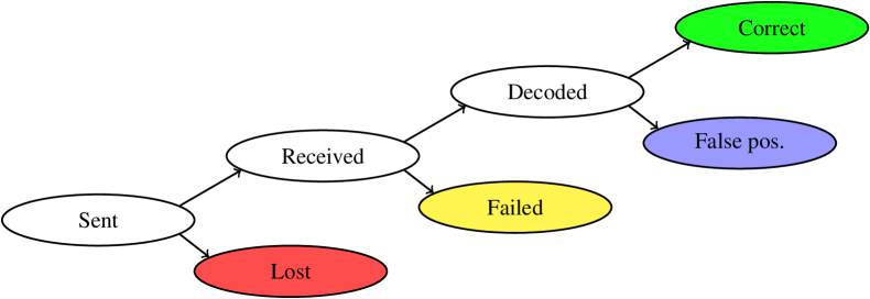
Figure 8: Classification of packets for the bar graph test.

We then used two further nodes to receive data from the predecessor set. The first one was located at a distance of $5\,$m with respect to the transmitting setup, the other at $60\,$m. The choice of both a near and a far predecessor further generalizes the results.

The test involved sending roughly $6\cdot 10^{5}$ packets, divided in all the possible combination of transmission skew between the equally powerful transmitters, in the set $\{80\,$ns, $160\,$ns, $320\,$ns, $640\,$ns$\}$, and interferer power in the set $\{$off, $-18\,$dBm, $-7\,$dBm, $-2\,$dBm$\}$. As illustrated by the decision tree represented in Figure 8, the outcomes of said transmissions are classified in four categories:

• correct, decoded and yielding a response within the values transmitted by the predecessor set nodes;

• false positive, causing the decoding algorithm to succeed but to output a number not in the expected range (most frequently, matching the interferer);

• failed, causing the algorithm to report the packet as too corrupted to be decoded;

• lost, not received for any reason.

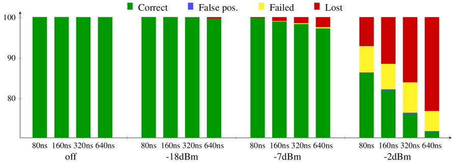
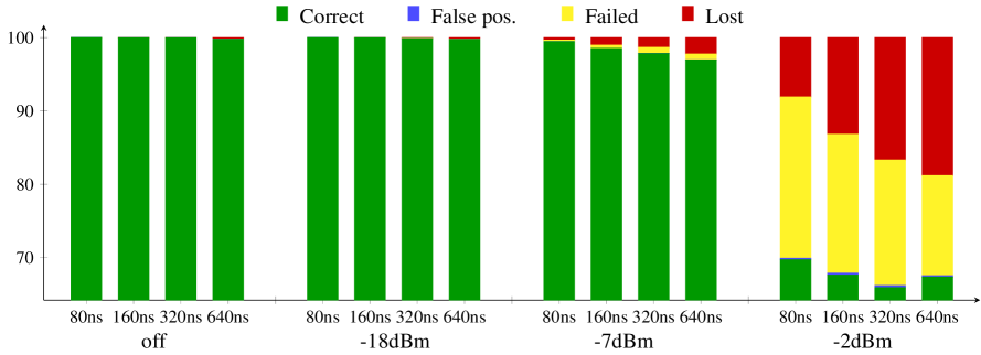
Figure 9: Bar graph test – receiver node placed at 5m from the transmitter, 16 bytes payload (top) and 64 bytes payload (bottom).

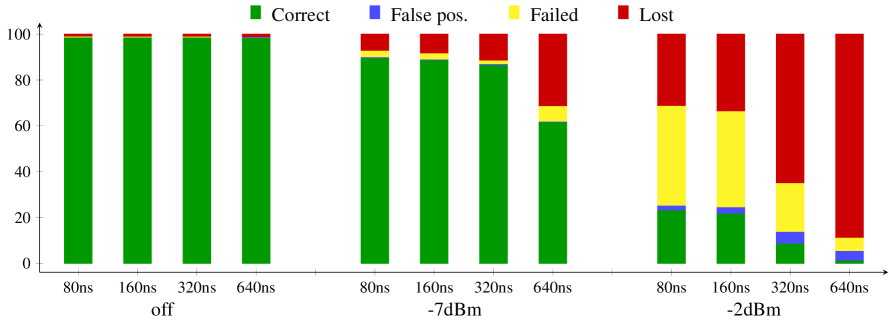
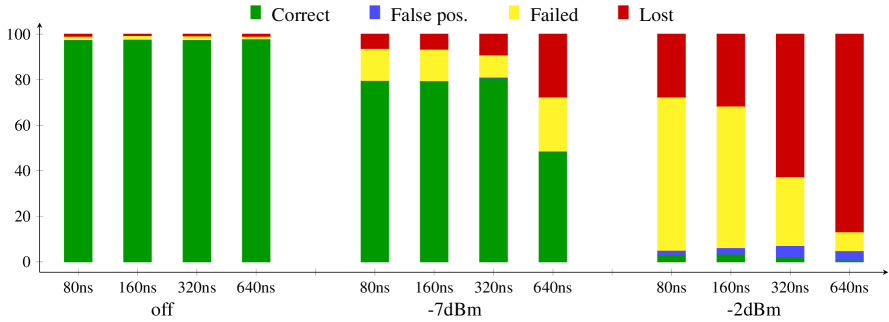
Figure 10: Bar graph test – receiver node placed at 60m from the transmitter, 16 bytes payload (top) and 64 bytes payload (bottom).

Results are reported as the percentage of packets falling into each category. Figure 9 shows the result for a node distance of $5\,$m with a packet length of 16 and 64 Bytes, while Figure 10 (mind the different vertical scales) reports the results for a $60\,$m distance. In Figure 10 the power of $-18\,$dBm is not reported as this would be equivalent to putting the interferer outside the radio range of the receiver, thus to the off case.

Considering the results for the $5\,$m distance, when the interfering power is compatible with a significant distance difference (up to $-7\,$dBm) and the transmission skew is within the Glossy tolerance of $0.5\,\mu$s [27], more than 97% of the packets are decoded correctly, regardless of payload length. Results for the $60\,$m distance show a more relevant difference between short and long packets, with the 16 Bytes case resulting in at least 86% correct packet reception, and the 64 Bytes dropping to a minimum of 80%.

Indeed, the technique fails only if either of the conditions above is violated. However, a skew above $500\,\mu$s would undermine the applicability of the Glossy flooding scheme itself, and can be easily avoided with a well timed packet retransmission delay. For what concerns a comparable power interferer, this is ruled out by geometrical reasons. In detail, using a model for the attenuation of radio waves in air [2], a node to have a $-2\,$dB difference from a node at $5\,$m from the receiver would need to be located at $6.3\,$m, thus having a distance from the predecessor set of only $1.3\,$m. In such a case, its propagation delay would not be different from the other nodes in the predecessor set, and thus it would not send a packet with a different number causing interference. Applying the same reasoning to the case where nodes are spaced $60\,$m apart results in the node sending at $-2\,$dBm being $15.5\,$m apart from the predecessor set, a difference of less than two timer ticks. Also in this case, the node would not cause interference. In practice, therefore, we can rule out the failing conditions.

VI-D Assessing the full scheme

The last experiment considers the integration of the proposed propagation delay compensator with a clock synchronization scheme, to assess the achieved improvement. A total of seven nodes were used for this test, using the FLOPSYNC-2 scheme configured with the default parameters for indoor use, a the synchronization period of $60\,$s, and $\alpha=3/8$ [1].

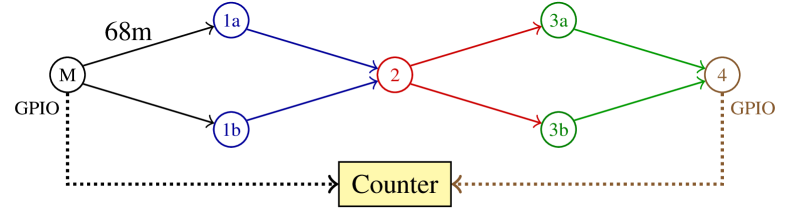
Figure 11: Network topology for the full scheme assessment.

The logical network topology of the setup is described in Figure 11. This setup was chosen to have a significant cumulated propagation delay from the master node to the last hop. Moreover, two nodes were employed for Hop 1 and 3 to test the effect of constructive interference in round-trip packet exchanges. For this experiment the flooding scheme was slightly altered, to force in software the network topology by manually assigning each node to a hop. This allowed to fold the logical topology in order to have the master node and node 4 physically next to each other, while forcing the flooded packets to follow the entire $272\,$m path. The application software running on the network periodically raised a pin on the microcontroller (in a hardware timed way, avoiding software jitter) at prescribed intervals. Having the master and last node close together allowed to connect their pins to an SR620 frequency counter, configured in time interval measurement mode to log the clock synchronization error. This counter has a sub-nanosecond resolution, far less than the measured time intervals.

TABLE I: Clock synchronization error at the fourth hop with and without propagation delay compensation.

	average	standard deviation
plain FLOPSYNC-2	1020 ns	696 ns
enhanced FLOPSYNC-2	0114 ns	687 ns

The experiment was repeated with the both plain FLOPSYNC-2, and with FLOPSYNC-2 enhanced with the proposed propagation delay compensation scheme. Table I shows how the lack of propagation delay compensation causes the synchronization error of plain FLOPSYNC-2 to exceed $1\,\mu$s, while the enhanced version remains well into the sub-microsecond region. The standard deviation does not increase significantly by propagation delay estimation. Incidentally, the difference between the two averages multiplied by the speed of radio waves in air amounts to $271.7\,$m, a value remarkably close to the actual node distance.

VII Related work

Time synchronization protocols can be broadly categorized in two classes: pairwise-synchronization schemes and flooding-based schemes. TPSN [24] is one of the most famous examples belonging to the first class. TPSN needs to construct a spanning tree of the network, and then performs synchronization along the edges. This increases the overhead in terms of packet transmissions and thus energy consumption, since packets should be sent for the spanning tree creation and maintenance. The availability of a spanning tree gives an explicit predecessor information and allows in principle to estimate the propagation delay, although this was not done as timestamping resolution was too limited when the paper was published. The second class, of which FTSP [22] is the precursor, is based on broadcast messages, transmitted by a master node to the neighboring ones and re-broadcast by the receivers for nodes that are not in the master node radio range. Flooding-based schemes are used because of their energy efficiency, since a single transmission can synchronize multiple nodes simultaneously. Optimized flooding schemes like Glossy [27] are crucial for this approach. However, flooding based schemes have the disadvantage that nodes do not know how the network is composed and therefore cannot easily compensate for the propagation delay. Our proposal provides an efficient solution to this issue.

Some alternative techniques have been proposed to combine the best of both worlds. Zeng et al. [21] proposed a measurement architecture using distributed air sniffers, which provides convenient transmission delay measurement, and requires no clock synchronization or instrumentation at the node level. The problem of sniffer placement still remains NP-hard [4], and the algorithms proposed cannot be applied to large WSNs. Saifullah et al. [9] analyze the effect of network delays on WirelessHART networks. This is a specific case of WSN for industrial process monitoring and control [25, 29, 12, 10, 19]. The proposed analysis methods are however focused on obtaining upper bounds on the end-to-end delay of every real-time periodic data flow in a WSN. These contributions further highlight the importance of efficiently estimating propagation delays in the network.

The problem of estimating propagation delays in wireless communication has been studied also in different areas, especially in underwater acoustic sensor networks [31, 7, 28], and satellite communication [11, 20]. The solutions proposed for these domains are exploiting the entity of the delays – exceeding the millisecond time scale – to improve the channel capacity. The problem that we faced in this paper is conversely to compensate for sub-microsecond delays in order to improve clock synchronization accuracy.

In this paper we have used interference to extract information from colliding packets. Collisions were also used to achieve indoor localization, leveraging capture effect [18]. The idea of exploiting interference is similar to the one presented in [30], where the initiator of a broadcast communication is able decode the superposition of ACK packets thanks to the constructive interference, although this case is simpler as all interfering packets have the same payload.

Katti et al. [15] proposed a technique called Analog Network Coding (ANC), that exploits signals transmission instead of packet transmission, with a similar attitude to our solution. Instead of trying to avoid interference in communication, they exploit it to increase the channel capacity. ANC is based on the idea that two senders can simultaneously send different packets on the channel, allowing packets collision. Since in ANC signals are transmitted, the collision of two signals results in a signal corresponding to their sum. The main limitation of this approach is that of requiring a software-defined radio to gain access to the received signal and disentangle the received packets. Our bar graph encoding, conversely, works with commodity radio transceivers. In addition, ANC is limited to the case of only two senders, while our proposal does not impose restriction on the cardinality of the predecessor set.

VIII Conclusion

In this paper we proposed a strategy to estimate the propagation delay in a WSN without the need to construct a spanning tree for the network. Our strategy is based on a custom encoding of the cumulated propagation delay that allows us to exploit the constructive transmission interference also to send similar packets. Our estimation strategy is here used to enhance flooding-based synchronization schemes with a delay compensator. We implemented our strategy on top of the FLOPSYNC-2 synchronization scheme [1], achieving sub-microsecond clock synchronization even in networks where propagation delays are significant.

References

- [1] F. Terraneo, L. Rinaldi, M. Maggio, A. V. Papadopoulos, and A. Leva. FLOPSYNC-2: Efficient monotonic clock synchronisation. RTSS, pages 11–20, 2014.
- [2] S. Saunders and A. Aragón-Zavala. Antennas and Propagation for Wireless Communication Systems: 2nd Edition. Wiley, 2007.
- [3] Hongwei Zhang, A. Arora, and P. Sinha. Learn on the fly: Data-driven link estimation and routing in sensor network backbones. INFOCOM, pages 1–12, 2006.
- [4] Wei Zeng, Xian Chen, Yoo-Ah Kim, Zhengming Bu, Wei Wei, Bing Wang, and Z.J. Shi. Delay monitoring for wireless sensor networks: An architecture using air sniffers. MILCOM, pages 1–8, 2009.
- [5] K. Leentvaar and J. Flint. The capture effect in fm receivers. IEEE Trans. on Communications, 24(5):531–539, 1976.
- [6] Su Ping. Delay measurement time synchronization for wireless sensor networks. In Intel Research, 2003.
- [7] Jianxiong Wen, Lianghui Ding, Feng Yang, Liang Qian, and Chuan Sun. Improved multi-hop time synchronization for underwater acoustic networks. WCSP, pages 1–6, 2013.
- [8] M.D. McDonnell. Is electrical noise useful? [point of view]. Proceedings of the IEEE, 99(2):242–246, 2011.
- [9] A. Saifullah, You Xu, Chenyang Lu, and Yixin Chen. End-to-end delay analysis for fixed priority scheduling in wirelesshart networks. RTAS, pages 13–22, 2011.
- [10] Giorgio Buttazzo. Research trends in real-time computing for embedded systems. SIGBED Rev., 3(3), 2006.
- [11] Li Gun and Huang Feijiang. Precise two way time synchronization for distributed satellite system. FREQ, pages 1122–1126, 2009.
- [12] Chenyang Lu, John A. Stankovic, Sang H. Son, and Gang Tao. Feedback control real-time scheduling: Framework, modeling, and algorithms. Real-Time Syst., 23(1/2):85–126, 2002.
- [13] Leslie Lamport. Time, clocks, and the ordering of events in a distributed system. Commun. ACM, 21(7):558–565, 1978.
- [14] Jeremy Elson, Lewis Girod, and Deborah Estrin. Fine-grained network time synchronization using reference broadcasts. SIGOPS Oper. Syst. Rev., 36(SI):147–163, 2002.
- [15] Sachin Katti, Shyamnath Gollakota, and Dina Katabi. Embracing wireless interference: Analog network coding. SIGCOMM, pages 397–408, New York, NY, USA, 2007. ACM.
- [16] H. Kopetz and W. Ochsenreiter. Clock synchronization in distributed real-time systems. IEEE Trans. Comput., 36(8):933–940, 1987.
- [17] Shucheng Liu, Guoliang Xing, Hongwei Zhang, Jianping Wang, Jun Huang, Mo Sha, and Liusheng Huang. Passive interference measurement in wireless sensor networks. ICNP, pages 52–61, 2010.
- [18] J. van Velzen and M. Zúñiga. Let’s collide to localize: Achieving indoor localization with packet collisions. PERCOM, pages 336–339, 2013.
- [19] Shan Lin, Gang Zhou, Mo’taz Al-Hami, Kamin Whitehouse, Yafeng Wu, John A. Stankovic, Tian He, Xiaobing Wu, and Hengchang Liu. Toward stable network performance in wireless sensor networks: A multilevel perspective. ACM Trans. Sen. Netw., 11(3):42:1–42:26, 2015.
- [20] Y. Kito, S. Kubota, F. Takahashi, T. Takahashi, T. Asai, and N. Katayama. First challenge of ptp time synchronization experiment through the experimental satellite for communication, ‘winds’. ISAP, pages 1493–1496, 2012.
- [21] Wei Zeng, Jordan Cote, Xian Chen, Yoo-Ah Kim, Wei Wei, Kyoungwon Suh, Bing Wang, and Zhijie Jerry Shi. Delay monitoring for wireless sensor networks: An architecture using air sniffers. Ad Hoc Networks, 13, Part B(0):549–559, 2014.
- [22] Miklós Maróti, Branislav Kusy, Gyula Simon, and Ákos Lédeczi. The flooding time synchronization protocol. SenSys, pages 39–49, 2004.
- [23] Carlo Alberto Boano, Thiemo Voigt, Nicolas Tsiftes, Luca Mottola, Kay Römer, and Marco Antonio Zúñiga. Making sensornet mac protocols robust against interference. In Wireless Sensor Networks, volume 5970, pages 272–288. 2010.
- [24] Saurabh Ganeriwal, Ram Kumar, and Mani B. Srivastava. Timing-sync protocol for sensor networks. SenSys, pages 138–149, 2003.
- [25] Tarek Abdelzaher, Yixin Diao, JosephL. Hellerstein, Chenyang Lu, and Xiaoyun Zhu. Introduction to control theory and its application to computing systems. In Performance Modeling and Engineering, pages 185–215. 2008.
- [26] Thomas Schmid, Prabal Dutta, and Mani B. Srivastava. High-resolution, low-power time synchronization an oxymoron no more. IPSN, pages 151–161, 2010.
- [27] F. Ferrari, M. Zimmerling, L. Thiele, and O. Saukh. Efficient network flooding and time synchronization with Glossy. IPSN, pages 73–84, 2011.
- [28] Pai-Han Huang, Maulik Desai, Xiaofan Qiu, and Bhaskar Krishnamachari. On the multihop performance of synchronization mechanisms in high propagation delay networks. IEEE Trans. Comp., 58(5):577–590, 2009.
- [29] Tian He, P. Vicaire, Ting Yan, Liqian Luo, Lin Gu, Gang Zhou, R. Stoleru, Qing Cao, J.A. Stankovic, and T. Abdelzaher. Achieving real-time target tracking usingwireless sensor networks. RTAS, pages 37–48, 2006.
- [30] Prabal Dutta, Razvan Musaloiu-E., Ion Stoica, and Andreas Terzis. Wireless ack collisions not considered harmful. HotNets, pages 19–24, 2008.
- [31] Peng Guo, Tao Jiang, Guangxi Zhu, and Hsiao-Hwa Chen. Utilizing acoustic propagation delay to design mac protocols for underwater wireless sensor networks. Wireless Comm. and Mobile Computing, 8(8):1035–1044, 2008.