Condensation of non-Abelian $SU(3)_{N_{f}}$ anyons in
a one-dimensional fermion model

Abstract

The color excitations of interacting fermions carrying an $SU(3)$ color and $U(N_{f})$ flavor index in one spatial dimension are studied in the framework of a perturbed $SU(3)_{N_{f}}$ Wess-Zumino-Novikov-Witten model. Using Bethe ansatz methods the low energy quasi-particles are found to be massive solitons forming $SU(3)$ quark and antiquark multiplets. In addition to the color index the solitons carry an internal degree of freedom with non-integer quantum dimension. These zero modes are identified as non-Abelian anyons satisfying $SU(3)_{N_{f}}$ fusion rules. Controlling the soliton density by external fields allows to drive the condensation of these anyons into various collective states. The latter are described by parafermionic cosets related to the symmetry of the system. Based on the numerical solution of the thermodynamic Bethe ansatz equations we propose a low temperature phase diagram for this model.

I Introduction

The remarkable properties of topological states of matter which cannot be characterized by a local order parameter but rather through their global entanglement properties have attracted tremendous interest in recent years. One particular consequence of the non-trivial bulk order is the existence of fractionalized quasi-particle excitations with unconventional statistics, so-called non-Abelian anyons. The ongoing search for physical realizations of these objects is driven by the possible utilization of their exotic properties, in particular in the quest for reliable quantum computing where the topological nature of non-Abelian anyons makes them a potentially promising resource Kitaev (2003); Nayak et al. (2008). Candidate systems supporting excitations with fractionalized zero energy degrees of freedom are the topologically ordered phases of two-dimensional quantum matter such as the fractional quantum Hall states or $p+ip$ superconductors Moore and Read (1991); Read and Rezayi (1999); Read and Green (2000). In these systems the presence of gapped non-Abelian anyons in the bulk leads to anomalous physics at the edges of the probe or at boundaries between phases of different topological order.

To characterize the latter it is essential to understand the properties of an ensemble of anyons where interactions lift the degeneracies of the anyonic zero modes and correlated many-anyon states are formed. One approach towards a classification of the possible collective states of interacting anyons has been to study effective lattice models Feiguin et al. (2007); Gils et al. (2013); Finch et al. (2014a, b); Braylovskaya et al. (2016); Vernier et al. (2017); Finch et al. (2018). Here the local degrees of freedom are objects in a braided tensor category with operations describing their fusion and braiding. Note that both the Hilbert space of the many-anyon system and the possible local interactions in the lattice model are determined by the fusion rules. These models allow for studies of many interacting anyons in one spatial dimension, both using numerical or, after fine-tuning of couplings to make them integrable, analytical methods thereby providing important insights into the collective behaviour of non-Abelian anyons. However, the question of how these degrees of freedom can be realized in a microscopic physical system is beyond its scope of this approach. In addition, the effective anyon models do not contain parameters, e.g. external fields, which would allow to drive a controlled transition from a phase with isolated anyons into a condensate.

Here we address these questions starting from a particular one-dimensional system of fermions: it is well known that strong correlations together with the quantum fluctuations in such systems may lead to the fractionalization of the elementary degrees of freedom of the constituents, the best-known example being spin-charge separation in correlated electron systems such as the one-dimensional Hubbard model Essler et al. (2005). A similar phenomenon can be observed in a system of spin-$1/2$ electrons with an additional orbital degree of freedom which is integrable by Bethe ansatz methods Tsvelik (2014); Borcherding and Frahm (2018): in the presence of a particularly chosen interaction the elementary excitations in the spin sector of this system are massive solitons (or kinks) connecting the different topological ground states of the model. On these kinks there are localized zero energy modes which, based on the exact low temperature thermodynamics, have been identified as spin-$1/2$ anyons satisfying $SU(2)_{k}$ fusion rules. The mass and density of the kinks (and therefore the anyons) can be controlled by the external magnetic field applied in the underlying electron system. This allows to study the condensation of the anyons into a the collective phase described by a parafermionic conformal field theory.

Below we extend this work by considering fermions forming an $SU(3)$ ’color’ and an additional $U(N_{f})$ flavor multiplet. We focus on the lowest energy excitations in the color subsector of the model in the presence of external fields coupled to the Cartan generators of the global $SU(3)$ symmetry. The spectrum of quasi-particles and the low temperature thermodynamics of the model are studied using Bethe ansatz methods. Using a combination of analytical methods and numerical solution of the nonlinear thermodynamic Bethe ansatz integral equations we identify anyonic zero modes which are localized on massive solitons in ’quark’ and ’antiquark’ color multiplets or bound states thereof. For sufficiently strong fields the mass gaps of the solitons close and the anyonic modes overlap. The resulting interaction lifts the degeneracy of the zero modes and the anyons condense into a phase with dispersing collective excitations whose low energy behaviour is described by parafermionic cosets. The transitions between the various topological phases realized by these anyons are signaled by singularities in thermodynamic quantities at low temperatures. These are signatures of anyon condensation, complementing similar studies of two-dimensional topological systems Levin and Wen (2005); Bais and Slingerland (2009); Haegeman et al. (2015); Iqbal et al. (2018).

II Integrability study of perturbed $\mathbf{SU(3)_{N_{f}}}$ WZNW model

We consider a system described by fermion fields forming a $SU(3)$ ’color’ multiplet and an auxiliary $U(N_{f})$ ’flavor’ multiplet. In the presence of weak interactions preserving the $U(1)$ charge, color, and flavor symmetries separately, conformal embedding can be used to split the Hamiltonian into a sum of three commuting parts describing the fractionalized degrees of freedom in the collective states Francesco et al. (1996). The non-Abelian color degrees of freedom are described in terms of a critical $SU(3)_{N_{f}}$ Wess-Zumino-Novikov-Witten model perturbed by current-current interactions with Hamiltonian density

$$\mathcal{H}=\frac{2\pi}{N_{f}+3}\left(:\mathbf{J}\cdot\mathbf{J}:+:\bar{\mathbf{J}}\cdot\bar{\mathbf{J}}:\right)+\lambda_{\parallel}\sum_{i=1}^{2}H^{i}\bar{H}^{i}+\lambda_{\perp}\sum_{\alpha>0}\frac{|\alpha|^{2}}{2}\left(E^{\alpha}\bar{E}^{-\alpha}+E^{-\alpha}\bar{E}^{\alpha}\right)\,.$$ (1)

Here $\mathbf{J}$ and $\bar{\mathbf{J}}$ are the right- and left-moving $SU(3)_{N_{f}}$ Kac-Moody currents. In terms of the corresponding fermion fields their components are

$$H^{i} =R^{\dagger}_{ak}(h^{i})_{ab}R_{bk}\,,\qquad E^{\alpha}=R^{\dagger}_{ak}(e^{\alpha})_{ab}R_{bk}\,,$$

$$\bar{H}^{i} =L^{\dagger}_{ak}(h^{i})_{ab}L_{bk}\,,\qquad\bar{E}^{\alpha}=L^{\dagger}_{ak}(e^{\alpha})_{ab}L_{bk}\,,$$

where $h^{i}$ $(i=1,2)$ are the generators of the $SU(3)$ Cartan subalgebra and $e^{\alpha}$ denote the ladder operator for the root $\alpha$ in the Cartan-Weyl basis ($1\leq a,b\leq 3$ and $1\leq k\leq N_{f}$ are color and flavor indices, respectively).

The spectrum of (1) can be obtained using Bethe ansatz methods, see e.g. Faddeev and Reshetikhin (1986); Babujian and Tsvelick (1986), based on the observation that the underlying structures coincide with those of an integrable deformation of the $SU(3)$ magnet with Dynkin label $(N_{f},0)$ Kulish and Reshetikhin (1981); Perk and Schultz (1981); Kulish et al. (1981); Babelon et al. (1982); Kulish and Reshetikhin (1983); Andrei and Johannesson (1984). Specifically, placing $\mathcal{N}=\sum\mathcal{N}_{\alpha}$ fermions into a box of length $L$ with periodic boundary conditions and applying magnetic fields $H_{1}$, $H_{2}$ coupled to the conserved charges the energy eigenvalues in the sector with $\mathcal{N}_{1}\geq\mathcal{N}_{2}\geq\mathcal{N}_{3}$ are

$$E=\frac{\mathcal{N}}{L}\sum_{\alpha=1}^{N_{1}}\sum_{\tau=\pm 1}\frac{\tau}{2\rm{i}}\ln\left(\frac{\sinh(\frac{\pi}{2p_{0}}(\lambda^{(1)}_{\alpha}+\tau/g-N_{f}\rm{i}))}{\sinh(\frac{\pi}{2p_{0}}(\lambda^{(1)}_{\alpha}+\tau/g+N_{f}\rm{i}))}\right)+N_{1}H_{1}+N_{2}H_{2}-\mathcal{N}\left(\frac{2}{3}H_{1}+\frac{1}{3}H_{2}\right)\,,$$ (2)

where $N_{1}=\mathcal{N}_{2}+\mathcal{N}_{3}$, $N_{2}=\mathcal{N}_{3}$, and the parameters $g$ and $p_{0}>N_{f}$ are functions of the coupling constants $\lambda_{\parallel}$ and $\lambda_{\perp}$. The relativistic invariance of the fermion model is broken by the choice of boundary conditions but will be restored later by considering observables in the scaling limit $L,\mathcal{N}\to\infty$ and $g\ll 1$ such that the mass of the elementary excitations is small compared to the particle density $\mathcal{N}/L$.

The energy eigenvalues (2) are parameterized by complex parameters $\lambda^{(m)}_{\alpha}$ with $\,\alpha=1,\dots,N_{m}$ and $m=1,2$ solving the hierarchy of Bethe equations (cf. Refs. Perk and Schultz (1981); Schultz (1983); de Vega and Lopes (1991); Lopes (1992) for the magnet in the fundamental representation, $N_{f}=1$)

$$\prod_{\tau=\pm 1}e_{N_{f}}(\lambda^{(1)}_{\alpha}+\tau/g)^{\mathcal{N}/2} =\prod_{\beta\neq\alpha}^{N_{1}}e_{2}(\lambda^{(1)}_{\alpha}-\lambda^{(1)}_{\beta})\prod_{\beta=1}^{N_{2}}e_{-1}(\lambda^{(1)}_{\alpha}-\lambda^{(2)}_{\beta})\,,\quad\alpha=1,\ldots,N_{1}$$ (3)

$$\prod_{\beta=1}^{N_{1}}e_{1}(\lambda^{(2)}_{\alpha}-\lambda^{(1)}_{\beta}) =\prod_{\beta\neq\alpha}^{N_{2}}e_{2}(\lambda^{(2)}_{\alpha}-\lambda^{(2)}_{\beta})\,,\quad\alpha=1,\ldots,N_{2}$$

where $e_{k}(x)=\sinh\left(\frac{\pi}{2p_{0}}(x+{\rm i}k)\right)/\sinh\left(\frac{\pi}{2p_{0}}(x-{\rm i}k)\right)$. Based on these equations the thermodynamics of the model can be studied provided that the solutions to the Bethe equations describing the eigenstates in the limit $\mathcal{N}\to\infty$ are known. Here we argue that the root configurations corresponding to the ground state and excitations relevant for the low temperature behaviour of (1) can be built based on the string hypothesis for the $U_{q}(sl(2))$ models Takahashi and Suzuki (1972), i.e. that in the thermodynamic limit the Bethe roots $\lambda_{\alpha}^{(m)}$ on both levels $m=1,2$ can be grouped into ’$j$-strings’ of length $n_{j}$ and with parity $v_{n_{j}}\in\{\pm 1\}$

$$\lambda^{(m)}_{j,\alpha,k}=\lambda^{(m)}_{j,\alpha}+i\left(n_{j}+1-2k+\frac{p_{0}}{2}(1-v_{N_{f}}v_{n_{j}})\right)\,,\quad\quad k=1,\dots,n_{j},\quad m=1,2\,,$$ (4)

with real centers $\lambda^{(m)}_{j,\alpha}\in\mathbb{R}$. The allowed lengths and parities depend on the parameter $p_{0}$. In the following we further simplify our discussion by assuming $p_{0}=N_{f}+1/\nu$ with integer $\nu>2$ where the following $N_{f}+\nu$ different string configurations contribute to the low temperature thermodynamics:

• $j_{0}=N_{f}+\nu$ with $(n_{j_{0}},v_{n_{j_{0}}})=(N_{f},+1)$,

• $j_{1}\in\{N_{f},N_{f}+1,\ldots N_{f}+\nu-1\}$ with $(n_{j_{1}},v_{n_{j_{1}}})=((j_{1}-N_{f})N_{f}+1,(-1)^{j_{1}+N_{f}+1})$,

• $j_{2}\in\{1,2,\ldots,N_{f}-1\}$ with $(n_{j_{2}},v_{n_{j_{2}}})=(j_{2},+1)$.

Within the root density approach the Bethe equations are rewritten as coupled integral equations for the densities of these strings Yang and Yang (1966). For vanishing magnetic fields one finds that the Bethe root configuration corresponding to the lowest energy state is described by finite densities of $j_{0}$-strings on both levels $m=1,2$. The elementary excitations above this ground state are of three types: similar as in the isotropic magnet Johannesson (1986) there are solitons or ’quarks’ and ’antiquarks’ corresponding to holes in the distributions of $j_{0}$-strings on level $m=1,2$. They carry quantum numbers in the fundamental representations $(1,0)$ and $(0,1)$ of $SU(3)$, respectively (independent of the representation $(N_{f},0)$ used for the construction of the spin chain). The $\nu$ different types of $j_{1}$-strings are called ’breathers’. Finally, there are auxiliary modes given by $j_{2}$-strings. The densities $\rho^{(m)}_{j}(\lambda)$ of these excitations (and $\rho^{h(m)}_{j}(\lambda)$ for the corresponding vacancies) satisfy the integral equations ($a\ast b$ denotes the convolution of $a$ and $b$)

$$\rho^{h(m)}_{k}(\lambda)={\rho}^{(m)}_{0,k}(\lambda)-\sum_{\ell=1}^{2}\sum_{j}\left(B^{(m,\ell)}_{kj}\ast\rho^{(\ell)}_{j}\right)(\lambda)\,,\qquad m=1,2\,,$$ (5)

see Appendix A. As mentioned above relativistic invariance is restored in the scaling limit $g\ll 1$ where the solitons are massive particles with bare densities ${\rho}^{(m)}_{0,j_{0}}(\lambda)$ and bare energies $\epsilon^{(m)}_{0,j_{0}}$

$${\rho}^{(m)}_{0,j_{0}}(\lambda) \stackrel{{\scriptstyle g\ll 1}}{{\simeq}}\frac{M_{0}}{6}\cosh(\pi\lambda/3)\,,$$ (6)

$${\epsilon}^{(m)}_{0,j_{0}}(\lambda) \stackrel{{\scriptstyle g\ll 1}}{{\simeq}}M_{0}\cosh(\pi\lambda/3)-\begin{cases}(Z_{1}H_{1}+Z_{2}H_{2})\,,\quad m=1,\\ (Z_{2}H_{1}+Z_{1}H_{2})\,,\quad m=2\,.\end{cases}$$

Here $M_{0}\equiv M_{j_{0}}=(2\mathcal{N}/L)\sin(\pi/3)e^{-\frac{\pi}{3g}}$ is the soliton mass while $Z_{1}=\frac{2}{3}(1+N_{f}\nu)$ and $Z_{2}=\frac{1}{3}(1+N_{f}\nu)$ parameterize the $SU(3)$ charges of these excitations corresponding to the highest weight states in the quark and antiquark representation. Similarly, breathers have bare densities and energies

$${\rho}^{(m)}_{0,j_{1}}(\lambda) \stackrel{{\scriptstyle g\ll 1}}{{\simeq}}\frac{M_{j_{1}}}{6}\cosh(\pi\lambda/3)\,,$$ (7)

$${\epsilon}^{(m)}_{0,j_{1}}(\lambda) \stackrel{{\scriptstyle g\ll 1}}{{\simeq}}M_{j_{1}}\cosh(\pi\lambda/3)-\begin{cases}(-1)^{m}Z_{2}(H_{1}-H_{2})\,,&\text{if }j_{1}=N_{f}+\nu-1,\\ (Z_{2}H_{1}+Z_{1}H_{2})\,,&\text{if }0\leq j_{1}-N_{f}<\nu-1\,,\,m=1,\\ (Z_{1}H_{1}+Z_{2}H_{2})\,,&\text{if }0\leq j_{1}-N_{f}<\nu-1\,,\,m=2\,,\end{cases}$$

with masses

$$M_{j_{1}} \equiv\begin{cases}2M_{0}\,\sin\left((j_{1}-N_{f}+1)\frac{\pi}{3\nu}+\frac{\pi}{6}\right)\,,&\text{if }0\leq j_{1}-N_{f}<\nu-1\,,\\ M_{0}\,,&\text{if }j_{1}=N_{f}+\nu-1\equiv\tilde{j}_{0}\,.\end{cases}$$ (8)

Note that the mass of the breathers with $j_{1}=\tilde{j}_{0}$ coincides with that of the solitons. The magnetic fields, however, couple to these modes in a different way, indicating that they are descendents of the $SU(3)$ highest weight states in the quark and antiquark multiplet. Therefore excitations of types $j_{0}$ and $\tilde{j}_{0}$ will both be labelled solitons (or quarks and antiquarks for solitons on level $m=1$ and $2$, respectively) below. The masses and $SU(3)$ charges of the auxiliary modes vanish, i.e. ${\rho}^{(m)}_{0,j_{2}}(\lambda)=0={\epsilon}^{(m)}_{0,j_{2}}(\lambda)$.

The energy density of a macro-state with densities given by (5) is

$$\Delta\mathcal{E}=\sum_{m=1}^{2}\sum_{j}\int_{-\infty}^{\infty}\text{d}\lambda\,{\epsilon}^{(m)}_{0,j}(\lambda)\rho^{(m)}_{j}(\lambda)\,.$$ (9)

III Low Temperature Thermodynamics

Additional insights into the physical properties of the different quasi-particles appearing in the Bethe ansatz solution of the model (1) can be obtained from its low temperature thermodynamics. The equilibrium state at finite temperature is obtained by minimizing the free energy, $F/\mathcal{N}=\mathcal{E}-T\mathcal{S}$, with the combinatorial entropy density Yang and Yang (1969)

$$\mathcal{S}=\sum_{m=1}^{2}\sum_{j}\int\text{d}\lambda\,\left[(\rho^{(m)}_{j}+\rho^{h(m)}_{j})\ln(\rho^{(m)}_{j}+\rho^{h(m)}_{j})-\rho^{(m)}_{j}\ln\rho^{(m)}_{j}-\rho^{h}_{j}\ln\rho^{h(m)}_{j}\right]\,.$$ (10)

The resulting thermodynamic Bethe ansatz (TBA) equations for the dressed energies $\epsilon_{j}^{(m)}(\lambda)=T\ln\left(\rho_{j}^{h(m)}(\lambda)/\rho_{j}^{(m)}(\lambda)\right)$ read

$$T\ln(1+e^{\epsilon^{(m)}_{k}/T})={\epsilon}^{(m)}_{0,k}(\lambda)+\sum_{\ell=1}^{2}\sum_{j}B^{(\ell,m)}_{jk}\ast T\ln(1+e^{-\epsilon^{(\ell)}_{j}/T}).$$ (11)

It is convenient to rewrite the equations for the auxiliary modes $j\in\{j_{2}\}$

$$\epsilon^{(m)}_{j_{2}}(\lambda)= s\ast T\ln(1+e^{\epsilon^{(m)}_{j_{2}+1}/T})(1+e^{\epsilon^{(m)}_{j_{2}-1}/T})-s\ast T\ln(1+e^{-\epsilon^{(3-m)}_{j_{2}}/T})\,,$$ (12)

$$\qquad j_{2}=1,\ldots,N_{f}-2\,,$$

$$\epsilon^{(m)}_{N_{f}-1}(\lambda)= s\ast T\ln(1+e^{\epsilon^{(m)}_{N_{f}-2}/T})-s\ast T\ln(1+e^{-\epsilon^{(3-m)}_{N_{f}-1}/T})$$

$$+\sum_{j\notin\{j_{2}\}}C^{(m)}_{j}\ast T\ln(1+e^{-\epsilon^{(m)}_{j}/T})\,,$$

where $\epsilon^{(m)}_{0}=-\infty$, $s(\lambda)=\frac{1}{4\cosh{\pi\lambda/2}}$ and the kernels $C^{(m)}_{j}$ are defined in Appendix A. Notice that the integral equations for the auxiliary modes (12) coincide with the integral equations of RSOS models of $A_{2}$ type up to the driving terms Bazhanov and Reshetikhin (1990). The free energy per particle in terms of the solutions to the TBA equations for the solitons and breathers as

$$\frac{F}{\mathcal{N}} \,\,=\,\,-T\sum_{m=1}^{2}\sum_{j\notin\{j_{2}\}}\int_{-\infty}^{\infty}\text{d}\lambda\,{\rho}^{(m)}_{0,j}(\lambda)\ln(1+e^{-\epsilon^{(m)}_{j}/T})\,$$ (13)

$$\stackrel{{\scriptstyle g\ll 1}}{{=}}-\frac{T}{6}\sum_{m=1}^{2}\sum_{j\notin\{j_{2}\}}M_{j}\int_{-\infty}^{\infty}\text{d}\lambda\,\cosh(\pi\lambda/3)\ln(1+e^{-\epsilon^{(m)}_{j}/T})\,.$$

Solving the TBA equations (11) we obtain the spectrum of the model (1) for given temperature $T$ and fields. In the following we restrict ourselves to the regime $H_{1}\geq H_{2}$ – exchanging $H_{1}\leftrightarrow H_{2}$ corresponds to interchanging the two levels of the Bethe ansatz. From the expressions (6) and (7) for the bare energies of the elementary excitations we can deduce the qualitative behaviour of these modes at low temperatures: As long as $Z_{1}H_{1}+Z_{2}H_{2}\lesssim M_{0}$ solitons and breathers remain gapped. Increasing the fields with $H_{1}>H_{2}$ the gap of the quarks ($m=1$ in (6)) closes once $Z_{1}H_{1}+Z_{2}H_{2}\simeq M_{0}$. For larger fields they condense into a phase with finite density $\rho^{(1)}_{j_{0}}$ and the degeneracy of the corresponding zero energy auxiliary modes is lifted. At even larger fields the gap of the $SU(3)$ highest weight state of the antiquark will close, too, and the systems enters a collective phase with a finite density of quarks and antiquarks. In Figures 1 and 2 the zero temperature mass spectrum for the model with $N_{f}=2$, $\nu=3$ is shown as function of $H_{1}$ for $H_{2}=0$ and $H_{1}=H_{2}$, respectively. Note that in the latter case the spectra of elementary excitations on level $1$ and $2$ coincide, $\epsilon^{(1)}_{j}\equiv\epsilon^{(2)}_{j}$ for all $j$.

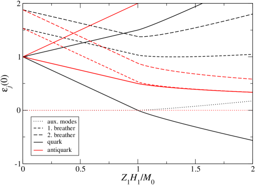
Figure 1: The energy gap of the elementary excitations (and Fermi energy of quarks in the condensed phase, respectively) $\epsilon^{(m)}_{j}(0)$ obtained from the numerical solution of (11) as a function of the field $H_{1}$ for $p_{0}=2+1/3$ at zero temperature and field $H_{2}=0$ (gaps on level $m=1$ ($2$) are displayed in black (red)). Note that in this case the high energy quark and the low energy antiquark levels are twofold degenerate. For $Z_{1}H_{1}=M_{0}$ the quark gap ($\epsilon^{(1)}_{j_{0}}(0)$) closes and the system forms a collective state of these objects. In this phase the degeneracy of the auxiliary modes is lifted. Increasing the field to $Z_{1}H_{1}\gg M_{0}$ the gaps of the antiquarks ($\epsilon^{(2)}_{j_{0}}(0)$ and $\epsilon^{(2)}_{\tilde{j}_{0}}(0)$) close. For small fields the low lying auxiliary modes are clearly separated from the spectrum of solitons and breathers.

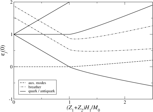
Figure 2: Same as Fig. 1 but for magnetic fields $H_{1}\equiv H_{2}$. In this case the elementary excitations for $m=1$ and $2$ are degenerate.

Based on this picture we now discuss the behaviour of the free energy as function of the fields at temperatures small compared to the relevant energy scales, i.e. the masses or Fermi energies of the solitons, $0<T\ll|Z_{1}H_{1}+Z_{2}H_{2}-M_{0}|$.

III.1 Non-interacting solitons

For fields $Z_{1}H_{1}+Z_{2}H_{2}\lesssim M_{0}$ solitons and breathers are gapped. At temperatures small compared to the gaps of the solitons the nonlinear integral equations (11) can be solved by iteration: the energies of the massive excitations are well described by their first order approximation Tsvelik (2014) while those of the auxiliary modes are given by the asymptotic solution of (12) for $|\lambda|\rightarrow\infty$ Kirillov (1989)

$$1+e^{\epsilon^{(m)}_{j_{2}}/T}=\frac{\sin\left(\frac{(j_{2}+1)\pi}{N_{f}+3}\right)\sin\left(\frac{(j_{2}+2)\pi}{N_{f}+3}\right)}{\sin\left(\frac{\pi}{N_{f}+3}\right)\sin\left(\frac{2\pi}{N_{f}+3}\right)}\,.$$ (14)

For solitons and breathers this implies ($Q\equiv 1+e^{\epsilon^{(1)}_{1}}=\frac{\sin(3\pi/(N_{f}+3))}{\sin(\pi/(N_{f}+3))}$)

$$\epsilon^{(m)}_{j}(\lambda)=\begin{cases}\tilde{\epsilon}^{(0,m)}_{j}(\lambda)-T\ln Q\qquad&j=j_{0},\tilde{j}_{0}\\ \tilde{\epsilon}^{(0,m)}_{j}(\lambda)-T\ln Q^{2}\quad&j\in\{j_{1}\}\setminus\{\tilde{j}_{0}\}\end{cases}$$ (15)

resulting in the free energy

$$\frac{F}{\mathcal{N}}= -\sum_{m=1}^{2}\sum_{j=j_{0},\tilde{j}_{0}}TQ\int\frac{\text{d}p}{2\pi}\,e^{-\left({\epsilon}^{(m)}_{0,j}(0)-p^{2}/2M_{0}\right)/T}-\sum_{m=1}^{2}\sum_{j\in\{j_{1}\}\setminus\{\tilde{j}_{0}\}}TQ^{2}\int\frac{\text{d}p}{2\pi}e^{-\left({\epsilon}^{(m)}_{0,j}(0)-p^{2}/2M_{j}\right)T}\,.$$ (16)

As observed in Refs. Tsvelik (2014); Borcherding and Frahm (2018) each of the terms appearing in this expression is the free energy of an ideal gas of particles with the corresponding mass carrying an internal degree of freedom with non-integer ’quantum dimension’ $Q$ for the solitons and $Q^{2}$ for the breathers ($j_{1}\neq\tilde{j}_{0}$). Their densities

$$n_{j}=\begin{cases}Q\sqrt{\frac{M_{0}T}{2\pi}}e^{-{\epsilon}^{(m)}_{0,j}(0)/T}\qquad&j=j_{0},\tilde{j}_{0},\\ Q^{2}\sqrt{\frac{M_{j}T}{2\pi}}e^{-{\epsilon}^{(m)}_{0,j}(0)/T}\qquad&j\in\{j_{1}\}\setminus\{\tilde{j}_{0}\}\end{cases}$$ (17)

can be controlled by variation of the temperature and the fields, which act as chemical potentials.

For the interpretation of this observation we consider fields $H_{1}>H_{2}$ and $Z_{1}H_{1}+Z_{2}H_{2}\lesssim M_{0}$ where the dominant contribution to the free energy is that of the lowest energy quarks, $j=j_{0}$, $m=1$. Their degeneracy $Q$ coincides with the quantum dimension of the anyons satisfying $SU(3)_{N_{f}}$ fusion rules with topological charge $[1,0]$ or $[1,1]$

$$d_{N_{f}}([x_{1},x_{2}])=\frac{\sin\left(\frac{\pi(x_{1}+2)}{N_{f}+3}\right)\,\sin\left(\frac{\pi(x_{2}+1)}{N_{f}+3}\right)\,\sin\left(\frac{\pi(x_{1}-x_{2}+1)}{N_{f}+3}\right)}{\sin\left(\frac{\pi}{N_{f}+3}\right)\,\sin\left(\frac{\pi}{N_{f}+3}\right)\,\sin\left(\frac{2\pi}{N_{f}+3}\right)}\,,$$ (18)

see Refs. Bazhanov and Reshetikhin (1990); Frahm and Karaiskos (2015); Schoutens and Wen (2016). Here $[x_{1},x_{2}]$ denotes the Young diagram with $x_{i}$ nodes in the $i$-th row. Following the discussion in Ref. Tsvelik (2014) we interpret this as a signature for the presence of $SU(3)_{N_{f}}$ anyonic zero modes bound to the quarks. The degeneracy $Q^{2}$ of the breather can be understood as a consequence of the breather being a bound state of two quarks, each contributing a factor $Q$ to the quantum dimension: from the fusion rule for $SU(3)_{N_{f}}$ $[1,0]$ and $[1,1]$ anyons,

$$[1,0]\times[1,0]=[1,1]+[2,0]\,,\quad[1,1]\times[1,1]=[1,0]+[2,2]\,,$$

for $N_{f}>1$, the degeneracy of this bound state is obtained to be $Q^{2}=d_{N_{f}}([1,1])+d_{N_{f}}([2,0])=d_{N_{f}}([1,0])+d_{N_{f}}([2,2])$.

III.2 Condensate of quarks

For fields $Z_{1}H_{1}\gtrsim M_{0}-Z_{2}H_{2}>\frac{2}{3}M_{0}$ the quarks in the $SU(3)$ highest weight state form a condensate, while the contribution to the free energy of the other solitons and the breathers can be neglected. For large fields $Z_{1}H_{1}\gg M_{0}-Z_{2}H_{2}$ the low temperature thermodynamics in this regime can be studied analytically: following Kirillov and Reshetikhin (1987) we observe that the dressed energies and densities can be related as

$$\rho^{(m)}_{j}(\lambda) =(-1)^{\delta_{j\in\{j_{2}\}}}\frac{1}{2\pi}\frac{\text{d}\epsilon^{(m)}_{j}(\lambda)}{\text{d}\lambda}f\left(\frac{\epsilon^{(m)}_{j}(\lambda)}{T}\right),$$ (19)

$$\rho^{h(m)}_{j}(\lambda) =(-1)^{\delta_{j\in\{j_{2}\}}}\frac{1}{2\pi}\frac{\text{d}\epsilon^{(m)}_{j}(\lambda)}{\text{d}\lambda}\left(1-f\left(\frac{\epsilon^{(m)}_{j}(\lambda)}{T}\right)\right)\,,$$

for $\lambda>\lambda_{\delta}$ with a sufficiently large $\exp(\pi\lambda_{\delta}/2)\gg 1$. $f(\epsilon)=1/(1+e^{\epsilon})$ is the Fermi function. Inserting this into (10) we get ($\phi^{(m)}_{j}=\epsilon^{(m)}_{j}/T$)

$$\mathcal{S}= -\frac{T}{\pi}\sum_{m,j}(-1)^{\delta_{j\in\{j_{2}\}}}\int_{\phi^{(m)}_{j}(\lambda_{\delta})}^{\phi^{(m)}_{j}(\infty)}\text{d}\phi^{(m)}_{j}\,\left[f(\phi^{(m)}_{j})\ln f(\phi^{(m)}_{j})+(1-f(\phi^{(m)}_{j}))\ln(1-f(\phi^{(m)}_{j}))\right]\,$$ (20)

$$+\sum_{m,j}\mathcal{S}^{(m)}_{j}(\lambda_{\delta})\,,$$

$$\mathcal{S}^{(m)}_{j} (\lambda_{\delta})\equiv\int_{-\lambda_{\delta}}^{\lambda_{\delta}}\text{d}\lambda\,\left[(\rho^{(m)}_{j}+\rho^{h(m)}_{j})\ln(\rho^{(m)}_{j}+\rho^{h(m)}_{j})-\rho^{(m)}_{j}\ln\rho^{(m)}_{j}-\rho^{h(m)}_{j}\ln\rho^{h(m)}_{j}\right]\,.$$

The integrals over $\phi^{(m)}_{j}$ can be performed giving

$$\mathcal{S}=\sum_{m,j}\mathcal{S}^{(m)}_{j}(\lambda_{\delta})-\frac{2T}{\pi}\sum_{m,j}(-1)^{\delta_{j\in\{j_{2}\}}}[L(f(\phi^{(m)}_{j}(\infty))-L(f(\phi^{(m)}_{j}(\lambda_{\delta})))].$$ (21)

in terms of the Rogers dilogarithm $L(x)$

$$L(x)=-\frac{1}{2}\int_{0}^{x}\text{d}y\,\left(\frac{\ln y}{1-y}+\frac{\ln(1-y)}{y}\right)\,.$$ (22)

In the regime considered here, i.e. $T\ll Z_{1}H_{1}+Z_{2}H_{2}-M_{0}$ and $\log((Z_{1}H_{1}+Z_{2}H_{2})/M_{0})>\lambda_{\delta}\gg 1$, we conclude from (11),(12) that

$$f(\phi^{(m)}_{j_{0}}(\lambda_{\delta}))=\begin{cases}1&m=1\\ 0&m=2\end{cases}, f(\phi^{(m)}_{j_{0}}(\infty)) =0,$$ (23)

$$f(\phi^{(m)}_{j_{1}}(\lambda_{\delta}))=0, f(\phi^{(m)}_{j_{1}}(\infty)) =0,$$

$$f(\phi^{(m)}_{j_{2}}(\lambda_{\delta}))=\begin{cases}0&m=1\\ \left(\frac{\sin(\frac{\pi}{N_{f}+2})}{\sin(\frac{\pi(j_{2}+1)}{N_{f}+2})}\right)^{2}&m=2\end{cases}, f(\phi^{(m)}_{j_{2}}(\infty)) =\frac{\sin(\frac{\pi}{N_{f}+3})\sin(\frac{2\pi}{N_{f}+3})}{\sin(\frac{j_{2}\pi}{N_{f}+3})\sin(\frac{(j_{2}+1)\pi}{N_{f}+3})},$$

and therefore

$$\rho^{h(1)}_{j_{0}}(\lambda)=\rho^{(2)}_{j_{0}}(\lambda)=\rho^{(m)}_{j_{1}}(\lambda)=\rho^{(1)}_{j_{2}}=0\quad$$ (24)

for $|\lambda|<\lambda_{\delta}$. Using $\rho^{(2)}_{j_{2}}(\lambda)=e^{-\epsilon^{(2)}_{j_{2}}/T}\rho^{h(2)}_{j_{2}}(\lambda)$ the integral equations (5) for $\rho^{h(2)}_{j_{2}}$ simplify in this regime to

$$\rho^{h(2)}_{j_{2}}=-\sum_{k_{2}}B^{(2,2)}_{j_{2}k_{2}}\ast e^{-\epsilon^{(2)}_{k_{2}}/T}\rho^{h(2)}_{k_{2}}\qquad\text{for }|\lambda|<\lambda_{\delta},$$ (25)

we conclude that $\rho^{h(2)}_{j_{2}}\rightarrow 0,$ $\rho^{(2)}_{j_{2}}\rightarrow 0$ such that $\rho^{(2)}_{j_{2}}/\rho^{h(2)}_{j_{2}}=e^{-\epsilon^{(2)}_{j_{2}}/T}=\text{const}$ for $|\lambda|<\lambda_{\delta}$ Consequently, we get $\mathcal{S}^{(m)}_{j}(\lambda_{\delta})=0$ for all $j,m$. Using $L(1)=\pi^{2}/6$ and the relation with ($N,N_{f}\geq 2$)

$$\sum_{m=1}^{N-1}\sum_{j_{2}=1}^{N_{f}-1}L\left(\frac{\sin(\frac{(N-m)\pi}{N_{f}+N})\sin(\frac{m\pi}{N_{f}+N})}{\sin(\frac{(N+j_{2}-m)\pi}{N_{f}+N})\sin(\frac{(j_{2}+m)\pi}{N_{f}+N})}\right)=\frac{\pi^{2}}{6}\left(\frac{N_{f}(N^{2}-1)}{N_{f}+N}-(N-1)\right)$$ (26)

for $N=2,3$ we get the following low-temperature behavior of the entropy

$$\mathcal{S}=\frac{\pi}{3}\left(\frac{8N_{f}}{N_{f}+3}-\frac{3N_{f}}{N_{f}+2}\right)T.$$ (27)

This is consistent with an effective description of the low energy collective modes in this regime through the coset $SU(3)_{N_{f}}/SU(2)_{N_{f}}$ conformal field theory with central charge

$$c=\frac{8N_{f}}{N_{f}+3}-\frac{3N_{f}}{N_{f}+2}.$$ (28)

Using the conformal embedding Castro-Alvaredo et al. (2000) (see also Huitu et al. (1990))

$$\frac{SU(3)_{N_{f}}}{SU(2)_{N_{f}}}=U(1)+\frac{Z_{SU(3)_{N_{f}}}}{Z_{SU(2)_{N_{f}}}},$$ (29)

where $Z_{SU(N)_{N_{f}}}=SU(N)_{N_{f}}/U(1)^{N}$ denotes generalized parafermions Gepner (1987), the collective modes can equivalently be described by a product of a free $U(1)$ boson contributing $c=1$ to the central charge and a parafermion coset $Z_{SU(3)_{N_{f}}}/Z_{SU(2)_{N_{f}}}$ contributing

$$c=\frac{8N_{f}}{N_{f}+3}-\frac{3N_{f}}{N_{f}+2}-1=\frac{6(N_{f}-1)}{N_{f}+3}-\frac{2(N_{f}-1)}{N_{f}+2}\,.$$ (30)

To study the transition from the gas of free anyons to the condensate of quarks described by the CFT (29) at intermediate fields $Z_{1}H_{1}\gtrsim M_{0}-Z_{2}H_{2}$ we have solved the TBA equations (11) numerically. Similar as in Ref. Borcherding and Frahm (2018) this can be done choosing suitable initial distributions and iterating the integral equations for given fields $H_{1},H_{2}$, temperature $T$ and anisotropy parameter $p_{0}$.

Using (13) the entropy can be computed from the numerical data as

$$\mathcal{S} =-\frac{\text{d}}{\text{d}T}\frac{F}{\mathcal{N}}$$ (31)

$$=\sum_{m,j\notin\{j_{2}\}}\frac{M_{j}}{4}\int\text{d}\lambda\,\cosh\left(\frac{\pi\lambda}{2}\right)\left(\log\left(1+e^{-\epsilon^{(m)}_{j}/T}\right)+\left(\frac{\epsilon^{(m)}_{j}}{T}-\frac{\text{d}}{\text{d}T}\epsilon^{(m)}_{j}\right)\left(1+e^{\epsilon^{(m)}_{j}/T}\right)^{-1}\right).$$

From the numerical solution of the TBA equations one finds that the low energy behaviour is determined by the quarks and the auxiliary modes on the first level which propagate with Fermi velocities

$$v^{(1)}_{\text{quark}}=\left.\frac{\partial_{\lambda}\epsilon^{(1)}_{j_{0}}}{2\pi\rho^{h(1)}_{j_{0}}}\right|_{\Lambda}\,,\qquad v^{(1)}_{pf}=-\left.\frac{\partial_{\lambda}\epsilon^{(1)}_{j_{2}}(\lambda)}{2\pi\rho^{h(1)}_{j_{2}}(\lambda)}\right|_{\lambda\to\infty}\,,$$ (32)

where $\Lambda$ is defined by $\epsilon^{(1)}_{j_{0}}(\Lambda)=0$. Note that $v^{(1)}_{pf}$ is the same for all auxiliary modes $(j\in\{j_{2}\},m=1)$

The resulting low temperature entropy is the sum of contributions from a $U(1)$ boson (quark) and a $Z_{SU(3)_{N_{f}}}/Z_{SU(2)_{N_{f}}}$ parafermionic coset (from the auxiliary modes)

$$\mathcal{S}=\frac{\pi}{3}\left(\frac{1}{v^{(1)}_{\text{quark}}}+\frac{1}{v^{(1)}_{pf}}\left(\frac{6(N_{f}-1)}{N_{f}+3}-\frac{2(N_{f}-1)}{N_{f}+2}\right)\right)T\,.$$ (33)

This behavior is consistent with the conformal embedding (29). Note that both Fermi velocities depend on the field $H_{1}$ and approach $1$ as $H_{1}\gtrsim H_{1,\delta}$, see Fig. 3.

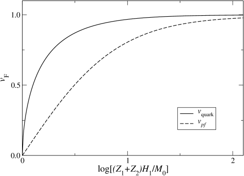
Figure 3: Fermi velocities of the quarks and first level $SU(3)$ parafermion modes as a function of the field $Z_{1}H_{1}>M_{0}$ for $p_{0}=2+1/3$, $H_{2}\equiv 0$ at zero temperature. For large fields, $H_{1}>H_{1,\delta}$, both Fermi velocities approach $1$ leading to the asymptotic result for the low temperature entropy (27).

Therefore, in this limit the entropy (27) of the coset $SU(3)_{N_{f}}/SU(2)_{N_{f}}$ is approached. In Fig. 4 the computed entropy (31) of the model with $N_{f}=2$, $\nu=3$ is shown for $T=0.01\,M_{0}$ as a function of the field $H_{1}$ together with the $T\to 0$ behaviour (33) expected from conformal field theory.

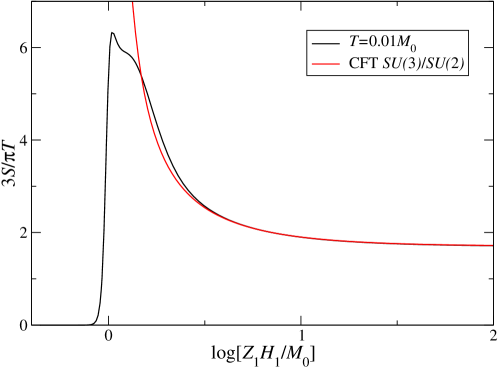
Figure 4: Entropy obtained from numerical solution of the TBA equations (11) for $p_{0}=2+1/3$ and $H_{2}\equiv 0$ as a function of the field $(Z_{1}H_{1}/M_{0}$ for $T=0.01M_{0}$. For fields large compared to the soliton mass, $Z_{1}H_{1}\gg M_{0}$, the entropy approaches the expected analytical value (27) for a field theory with a free bosonic sector and a $Z_{SU(3)_{N_{f}=2}}/Z_{SU(2)_{N_{f}=2}}$ parafermion sector propagating with velocities $v^{(1)}_{\text{quark}}$ and $v^{(1)}_{pf}$, respectively (full red line). For magnetic fields $Z_{1}H_{1}<M_{0}$ and temperature $T\ll M_{0}$ the entropy is that of a dilute gas of non-interacting quasi-particles with degenerate internal degree of freedom due to the anyons.

III.3 Condensate of quarks and antiquarks

For fields $H_{1}\geq H_{2}\gtrsim M_{0}/(Z_{1}+Z_{2})$ the system forms a collective state of solitons ($j=j_{0}$) on both levels, $m=1,2$. Again, the low temperature thermodynamics can be studied analytically for $H_{1}\geq H_{2}\gg M_{0}/(Z_{1}+Z_{2})$ . Repeating the analysis of Section III.2 we conclude from Eqs. (11), (12) that

$$f(\phi^{(m)}_{j_{0}}(\lambda_{\delta}))=\begin{cases}1\quad m=1,\\ 1\quad m=2\end{cases},\qquad f(\phi^{(m)}_{j_{0}}(\infty))=0,$$ (34)

$$f(\phi^{(m)}_{j_{1}}(\lambda_{\delta}))=0,\qquad\qquad\qquad\qquad\,f(\phi^{(m)}_{j_{1}}(\infty))=0,$$

$$f(\phi^{(m)}_{j_{2}}(\lambda_{\delta}))=\begin{cases}0\qquad m=1,\\ 0\qquad m=2\end{cases},\quad\,f(\phi^{(m)}_{j_{2}}(\infty))=\frac{\sin(\frac{\pi}{N_{f}+3})\sin(\frac{2\pi}{N_{f}+3})}{\sin(\frac{j_{2}\pi}{N_{f}+3})\sin(\frac{(j_{2}+1)\pi}{N_{f}+3})},$$

and therefore

$$\rho^{h(m)}_{j_{0}}(\lambda)=\rho^{(m)}_{j_{1}}(\lambda)=\rho^{(m)}_{j_{2}}=0,\quad\mathrm{for~{}}|\lambda|<\lambda_{\delta}\,,$$ (35)

giving $\mathcal{S}^{(m)}_{j}(\lambda_{\delta})=0$ for all $j,m$. Using the relation (26) the low-temperature behavior of the entropy is found to be

$$\mathcal{S}=\frac{\pi}{3}\left(2+\frac{6(N_{f}-1)}{N_{f}+3}\right)T=\frac{\pi}{3}\frac{8N_{f}}{N_{f}+3}T$$ (36)

in the phase with finite soliton density on both levels. The low energy excitations near the Fermi points $\epsilon^{(m)}_{j_{0}}(\pm\Lambda_{m})=0$ of the soliton dispersion propagate with velocities $v^{(m)}_{\text{quark/antiquark}}=\left.(\partial_{\lambda}\epsilon^{(1/2)}_{j_{0}})/(2\pi\rho^{(1/2)}_{j_{0}})\right|_{\Lambda_{1/2}}\to 1$ for fields $H_{m}>H_{m,\delta}$ such that $\Lambda_{m}(H_{m,\delta})>\lambda_{\delta}$. From this we conclude that the conformal field theory (CFT) describing the collective low energy modes is the $SU(3)$ WZNW model at level $N_{f}$ or, by conformal embedding Gepner (1987), a product of two free $U(1)$ bosons (contributing $c=2$ to the central charge) and the $SU(3)$ parafermionic coset $SU(3)/U(1)^{2}$ with central charge

$$c=\frac{6(N_{f}-1)}{N_{f}+3}\,.$$ (37)

For the transition between this regime and the phases where the antiquarks are gapped, see Section III.2, we have to resort to an numerical analysis of the TBA equations (11) again: in the case of equal fields, $H_{1}\equiv H_{2}$, where the corresponding modes on the two levels are degenerate we find that the solitons $\epsilon_{j_{0}}^{(m)}$ propagate with Fermi velocity $v_{\text{quark}}$ while the auxiliary modes $\epsilon_{j_{2}}^{(m)}$ propagate with velocity $v_{pf}$ (independent of $j_{2}=1,\ldots,N_{f}-1$), see Fig. 5.

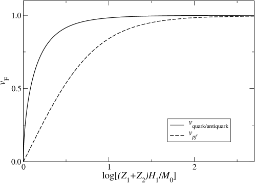
Figure 5: Fermi velocities of solitons and $SU(3)$ parafermion modes as a function of the magnetic field $H_{1}\equiv H_{2}>M_{0}(Z_{1}+Z_{2})$ for $p_{0}=2+1/3$ at zero temperature. For large fields, $H_{m}>H_{m,\delta}$, both Fermi velocities approach $1$ leading to the asymptotic result for the low temperature entropy (36).

As a consequence the contribution of the bosonic (quark/antiquark) and parafermionic degrees of freedom to the low temperature entropy separate into

$$\mathcal{S}=\frac{\pi}{3}\left(\frac{2}{v_{\text{quark}}}+\frac{1}{v_{pf}}\frac{6(N_{f}-1)}{N_{f}+3}\right)T\,.$$ (38)

In Fig. 6 the computed entropy (31) for the model $SU(3)_{N_{f}=2}$ model with $\nu=3$ is shown for various temperatures as a function of the fields $H_{1}\equiv H_{2}$ together with the $T\to 0$ behaviour (36) expected from conformal field theory.

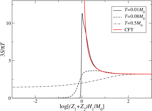
Figure 6: Same as Fig. 4 but for $H_{1}\equiv H_{2}$. For fields large compared to the soliton mass, $(Z_{1}+Z_{2})H_{1}\gg M_{0}$, the entropy approaches the expected analytical value (36) for a field theory with two free bosonic sectors and a $SU(3)$ parafermion sector propagating with velocities $v_{\text{quark}}=v_{\text{antiquark}}$ and $v_{pf}$, respectively (full red line). For magnetic fields $zH<M_{0}$ and temperature $T\ll M_{0}$ the entropy is that of a dilute gas of non-interacting quasi-particles with degenerate internal degree of freedom due to the $SU(3)_{N_{f}=2}$ anyons bound to the solitons.

Finally, in the regime $H_{1}\geq H_{2}\gtrsim M_{0}/(Z_{1}+Z_{2})$ the remaining degeneracy between the two levels is lifted. Quarks, antiquarks, and auxiliary modes are propagating with (generically) different Fermi velocities $v_{\text{quark}}$, $v_{\text{antiquark}}$, $v^{(1)}_{pf}$, and $v^{(2)}_{pf}$. The resulting low-temperature entropy behavior is found to be

$$\mathcal{S} =\frac{\pi}{3}\left(\frac{1}{v_{\text{quark}}}+\frac{1}{v_{\text{antiquark}}}+\frac{c_{1}}{v^{(1)}_{pf}}+\frac{c_{2}}{v^{(2)}_{pf}}\right)T,$$ (39)

$$c_{1} =\frac{6(N_{f}-1)}{N_{f}+3}-\frac{2(N_{f}-1)}{N_{f}+2}\,,\quad c_{2}=\frac{2(N_{f}-1)}{N_{f}+2},$$

consistent with the conformal embedding Castro-Alvaredo et al. (2000)

$$SU(3)_{N_{f}}=U(1)^{2}+Z_{SU(2)_{N_{f}}}+\frac{Z_{SU(3)_{N_{f}}}}{Z_{SU(2)_{N_{f}}}}.$$ (40)

Fig. 7 shows the transition between the different regimes described above.

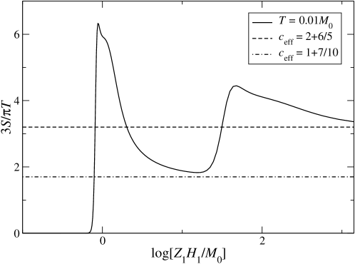
Figure 7: Same as Figure 4 but for fields along the line $\log(Z_{2}H_{2}/M_{0})\equiv 0.4\log(Z_{1}H_{1}/M_{0})-2.58$. Transitions are observed at fields where the quarks and antiquarks condense, i.e. from the low density phase of non-interacting anyons into the collective state described by the $SU(3)_{N_{f}=2}/SU(2)_{N_{f}=2}$ coset CFT at and later into a phase whose low energy description is in terms of the $SU(3)_{N_{f}=2}$ WZNW model. The dashed-dotted lines indicate the corresponding central charges.

IV Summary and Conclusion

We have studied the low temperature behaviour realized in a perturbed $SU(3)_{N_{f}}$ WZNW model based on the Bethe ansatz solution of the model describing the color sector of interacting fermions carrying color and flavor degrees of freedom. For small magnetic fields coupled to the $SU(3)$ charges the elementary excitations form quark and antiquark multiplets with finite mass carrying an internal non-Abelian $SU(3)_{N_{f}}$ anyonic degree of freedom. Varying the magnetic field quarks and antiquarks condense. As a result the non-Abelian degrees of freedom bound to the the soliton excitations begin to overlap. Their resulting interaction lifts the degeneracy of these modes resulting in the formation of various phases with propagating collective excitations. The effective theories describing these phases are products of Gaussian fields for the soliton degrees of freedom and parafermionic cosets. The latter describe the collective behaviour of interacting $SU(3)_{N_{f}}$ anyons related to the symmetries of the model. Our findings are summarized in Figure 8.

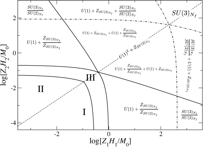
Figure 8: Contribution of the $SU(3)_{N_{f}}$ anyons to the low temperature properties of the model (1): using the criteria described in the main text the parameter regions are identified using analytical arguments for $T\to 0$ (the actual location of the boundaries is based on numerical data for $p_{0}=2+1/3$ and $T=0.05/M_{0}$). For small fields (regions I,II) a gas of non-interacting quasi-particles with the anyon as an internal zero energy degree of freedom bound to them is realized. Here the dashed line ($H_{1}\equiv H_{2}$ or $\epsilon^{(1)}_{j}\equiv\epsilon^{(2)}_{j}$) indicates the crossover between regions where the quarks (region I), or antiquarks (region II) dominate the free energy. In region III the presence of thermally activated solitons with a small but finite density lifts the degeneracy of the zero modes. The collective phases formed by condensed solitons are labelled by the corresponding CFTs providing the effective description of the low energy excitations.

Appendix A Thermodynamic Bethe ansatz

The fields $H_{1},H_{2}$ appearing in (2) are defined by $H_{1}\equiv\vec{\alpha}_{1}\cdot\vec{h}$, $H_{2}\equiv\vec{\alpha}_{2}\cdot\vec{h}$, where the fields $\vec{h}=(h_{1},h_{2})$ couple to the generators of the Cartan subalgebra of $SU(3)$ and $\vec{\alpha}_{1},\,\vec{\alpha}_{2}$ denote the simple roots of $SU(3)$.

In order to obtain the integral equations (5) we consider a root configuration consisting of $\nu^{(m)}_{j}$ strings of type $(n_{j},v_{n_{j}})$ on the $m-$th level and using (4) the Bethe equations (3) can be rewritten in terms of the real string-centers $\lambda^{(m,j)}_{\alpha}\equiv\lambda^{(m)n_{j}}_{\alpha}$. In their logarithmic form they read

$$\sum_{\tau=\pm 1}\frac{\mathcal{N}}{2}t_{k,N_{f}}(\lambda^{(1,k)}_{\alpha}+\tau/g) =2\pi I^{(1,k)}_{\alpha}+\sum_{j}\sum_{\beta=1}^{\nu^{(1)}_{j}}\theta^{(1)}_{kj}(\lambda^{(1,k)}_{\alpha}-\lambda^{(1,j)}_{\beta})-\sum_{j}\sum_{\beta=1}^{\nu^{(2)}_{j}}\theta^{(2)}_{kj}(\lambda^{(1,k)}_{\alpha}-\lambda^{(2,j)}_{\beta}),$$ (41)

$$0 =2\pi I^{(2,k)}_{\alpha}+\sum_{j}\sum_{\beta=1}^{\nu^{(2)}_{j}}\theta^{(1)}_{kj}(\lambda^{(2,k)}_{\alpha}-\lambda^{(2,j)}_{\beta})-\sum_{j}\sum_{\beta=1}^{\nu^{(1)}_{j}}\theta^{(2)}_{kj}(\lambda^{(2,k)}_{\alpha}-\lambda^{(1,j)}_{\beta}),$$

where $I^{(m,k)}_{\alpha}$ are integers (or half-integers) and we have introduced the functions

$$t_{k,N_{f}}(\lambda) =\sum_{l=1}^{\min(n_{k},N_{f})}f(\lambda,|n_{k}-N_{f}|+2l-1,v_{k}v_{N_{f}}),$$ (42)

$$\theta^{(1)}_{kj}(\lambda) =f(\lambda,|n_{k}-n_{j}|,v_{k}v_{j})+f(\lambda,n_{k}+n_{j},v_{k}v_{j})+2\sum_{\ell=1}^{\min(n_{k},n_{j})-1}f(\lambda,|n_{k}-n_{j}|+2\ell,v_{k}v_{j}),$$

$$\theta^{(2)}_{kj}(\lambda) =\sum_{l=1}^{\min(n_{k},n_{j})}f(\lambda,|n_{k}-n_{j}|+2l-1,v_{k}v_{j})$$

with

$$f(\lambda,n,v)=\begin{cases}2\arctan\left(\tan((\frac{1+v}{4}-\frac{n}{2p_{0}})\pi)\tanh(\frac{\pi\lambda}{2p_{0}})\right)\quad\text{if }\frac{n}{p_{0}}\neq\text{integer}\\ 0\hskip 193.47882pt\text{if }\frac{n}{p_{0}}=\text{integer}\end{cases}\,.$$

In the thermodynamic limit, $N_{m},\mathcal{N}\rightarrow\infty$ with $N_{m}/\mathcal{N}$ fixed, the centers $\lambda^{(m,k)}_{\alpha}$ are distributed continuously with densities $\rho^{(m)}_{k}(\lambda)$ and hole densities $\rho^{h(m)}_{k}(\lambda)$. Following Yang and Yang (1966) the densities are defined through the following integral equations

$$\tilde{\rho}^{(1)}_{0,k}(\lambda) =(-1)^{r(k)}\rho^{h(1)}_{k}(\lambda)+\sum_{j}A^{(1)}_{kj}\ast\rho^{(1)}_{j}(\lambda)-\sum_{j}A^{(2)}_{kj}\ast\rho^{(2)}_{j}(\lambda),$$ (43)

$$0 =(-1)^{r(k)}\rho^{h(2)}_{k}(\lambda)+\sum_{j}A^{(1)}_{kj}\ast\rho^{(2)}_{j}(\lambda)-\sum_{j}A^{(2)}_{kj}\ast\rho^{(1)}_{j}(\lambda),$$

where $a\ast b$ denotes a convolution and $r(j)$ is defined in Appendix A of Borcherding and Frahm (2018). The bare densities $\tilde{\rho}^{(1)}_{0,j}(\lambda)$ and the kernels $A^{(m)}_{jk}(\lambda)$ of the integral equations are defined by

$$\tilde{\rho}^{(1)}_{0,j}(\lambda) =\frac{1}{2}\left(a_{j,N_{f}}(\lambda+1/g)+a_{j,N_{f}}(\lambda-1/g)\right),\quad a_{j,N_{f}}(\lambda)=\frac{1}{2\pi}\frac{d}{d\lambda}t_{j,N_{f}}(\lambda)$$ (44)

$$A^{(m)}_{kj}(\lambda) =\frac{1}{2\pi}\frac{d}{d\lambda}\theta^{(m)}_{kj}(\lambda)+(-1)^{r(k)}\delta_{m1}\delta_{jk}\delta(\lambda)\,.$$

We rewrite the energy density $\mathcal{E}=E/\mathcal{N}$ using (2) and the solutions $\rho^{(m)}_{k}$ of (43) as

$$\mathcal{E} =\frac{1}{\mathcal{N}}\sum_{j}\sum_{\alpha=1}^{\nu^{(1)}_{j}}\left(\sum_{\tau=\pm 1}\frac{\tau}{2}t_{j,N_{f}}(\lambda^{(j,1)}_{\alpha}+\tau/g)+n_{j}H_{1}\right)+\frac{1}{\mathcal{N}}\sum_{j}\sum_{\alpha=1}^{\nu^{(2)}_{j}}n_{j}H_{2}-\frac{2}{3}H_{1}-\frac{1}{3}H_{2}$$ (45)

$$\stackrel{{\scriptstyle\mathcal{N}\rightarrow\infty}}{{=}}\sum^{2}_{m=1}\sum_{j\geq 1}\int_{-\infty}^{+\infty}\text{d}\lambda\,\tilde{\epsilon}^{(m)}_{0,j}(\lambda)\rho^{(m)}_{j}(\lambda)-\frac{2}{3}H_{1}-\frac{1}{3}H_{2},$$

where we introduced the bare energies

$$\tilde{\epsilon}^{(1)}_{0,j}(\lambda)=\sum_{\tau=\pm 1}\frac{\tau}{2}t_{j,N_{f}}(\lambda+\tau/g)+n_{j}H_{1},\quad\tilde{\epsilon}^{(2)}_{0,j}(\lambda)=n_{j}H_{2}.$$ (46)

It turns out that the energy (45) is minimized by a configuration, where only the strings of length $N_{f}$ have a finite density. After inverting the kernels $A^{(1)}_{j_{0}j_{0}}$ on both levels in equation (43) and inserting the resulting expression for $\rho^{(m)}_{j_{0}}(\lambda)$ into the other equations for $k\neq j_{0}$ we end up with the integral equations (5), where we redefined the densities $\rho^{h(m)}_{j_{0}}\leftrightarrow\rho^{(m)}_{j_{0}}$ and introduced the kernels $B^{(1,1)}_{jk}=B^{(2,2)}_{jk}\equiv B^{(1)}_{jk}$, $B^{(1,2)}_{jk}=B^{(2,1)}_{jk}\equiv B^{(2)}_{jk}$, whose Fourier transformed kernels $B^{(1)}_{jk}(\omega)$, $B^{(2)}_{jk}(\omega)$ are given by

$$B^{(m)}_{j_{0}j_{0}} =\frac{A^{(m)}_{j_{0}j_{0}}}{(A^{(1)}_{j_{0}j_{0}})^{2}-(A^{(2)}_{j_{0}j_{0}})^{2}},$$ (47)

$$B^{(m)}_{kj_{0}} =(-1)^{r(k)}\frac{A^{(2)}_{kj_{0}}A^{((m\text{ mod 2})+1)}_{j_{0}j_{0}}-A^{(1)}_{kj_{0}}A^{(m)}_{j_{0}j_{0}}}{(A^{(1)}_{j_{0}j_{0}})^{2}-(A^{(2)}_{j_{0}j_{0}})^{2}},\qquad k\neq j_{0},$$

$$B^{(m)}_{j_{0}k} =-(-1)^{r(k)}B^{(m)}_{kj_{0}},\qquad k\neq j_{0},$$

$$B^{(m)}_{kj} =(-1)^{r(k)}\left(A^{(2)}_{kj_{0}}B^{((m\text{ mod }2)+1)}_{j_{0}j}-A^{(1)}_{kj_{0}}B^{(m)}_{j_{0}j}+(-1)^{m+1}A^{(m)}_{kj}\right),\qquad k,j\neq j_{0}.$$

The inverse of the Fourier transformed kernel $B^{(1)}_{j_{2}k_{2}}(\omega)$ is given by $C_{j_{2}k_{2}}=\delta_{j_{2}k_{2}}-s(\delta_{j_{2}k_{2}+1}+\delta_{j_{2}k_{2}-1})$ Tsvelik (1987). Hence, the Fourier transformed kernels $C^{(m)}_{j}(\omega)$ of equation (12) are defined by

$$\sum_{j_{2}}C_{kj_{2}}B^{(1)}_{jj_{2}}=\delta_{k,N_{f}-1}C^{(m)}_{j}.$$ (48)

References

• Kitaev (2003) A. Yu. Kitaev, “Fault-tolerant quantum computation by anyons,” Ann. Phys. (NY) 303, 2–30 (2003), quant-ph/9707021 .
• Nayak et al. (2008) Chetan Nayak, Steven H. Simon, Ady Stern, Michael Freedman,  and Sankar Das Sarma, “Non-Abelian Anyons and Topological Quantum Computation,” Rev. Mod. Phys. 80, 1083–1159 (2008), arXiv:0707.1889 .
• Moore and Read (1991) Gregory Moore and Nicholas Read, “Nonabelions in the fractional quantum Hall effect,” Nucl. Phys. B 360, 362–396 (1991).
• Read and Rezayi (1999) N. Read and E. Rezayi, “Beyond paired quantum Hall states: parafermions and incompressible states in the first excited Landau level,” Phys. Rev. B 59, 8084–8092 (1999), cond-mat/9809384 .
• Read and Green (2000) N. Read and Dmitry Green, “Paired states of fermions in two dimensions with breaking of parity and time-reversal symmetries, and the fractional quantum Hall effect,” Phys. Rev. B 61, 10267 (2000), cond-mat/9906453 .
• Feiguin et al. (2007) Adrian Feiguin, Simon Trebst, Andreas W. W. Ludwig, Matthias Troyer, Alexei Kitaev, Zhenghan Wang,  and Michael H. Freedman, “Interacting anyons in topological quantum liquids: The golden chain,” Phys. Rev. Lett. 98, 160409 (2007), cond-mat/0612341 .
• Gils et al. (2013) Charlotte Gils, Eddy Ardonne, Simon Trebst, David A. Huse, Andreas W. W. Ludwig, Matthias Troyer,  and Zhenghan Wang, “Anyonic quantum spin chains: Spin-1 generalizations and topological stability,” Phys. Rev. B 87, 235120 (2013), arXiv:1303.4290 .
• Finch et al. (2014a) Peter E. Finch, Holger Frahm, Marius Lewerenz, Ashley Milsted,  and Tobias J. Osborne, “Quantum phases of a chain of strongly interacting anyons,” Phys. Rev. B 90, 081111(R) (2014a), arXiv:1404.2439 .
• Finch et al. (2014b) Peter E. Finch, Michael Flohr,  and Holger Frahm, “Integrable anyon chains: from fusion rules to face models to effective field theories,” Nucl. Phys. B 889, 299–332 (2014b), arXiv:1408.1282 .
• Braylovskaya et al. (2016) Natalia Braylovskaya, Peter E. Finch,  and Holger Frahm, “Exact solution of the D3subscriptđ·3{D}_{3} non-Abelian anyon chain,” Phys. Rev. B 94, 085138 (2016), arXiv:1606.00793 .
• Vernier et al. (2017) Eric Vernier, Jesper Lykke Jacobsen,  and Hubert Saleur, “Elaborating the phase diagram of spin-1 anyonic chains,” SciPost Phys. 2, 004 (2017), arXiv:1611.02236 .
• Finch et al. (2018) Peter E. Finch, Michael Flohr,  and Holger Frahm, “𝐙nsubscript𝐙𝑛\mathbf{Z}_{n} clock models and chains of s​o​(n)2𝑠𝑜subscript𝑛2so(n)_{2} non-Abelian anyons: symmetries, integrable points and low energy properties,” J. Stat. Mech. , 023103 (2018), arXiv:1710.09620 .
• Essler et al. (2005) Fabian H. L. Essler, Holger Frahm, Frank Göhmann, Andreas KlĂŒmper,  and Vladimir E. Korepin, The One-Dimensional Hubbard Model (Cambridge University Press, Cambridge (UK), 2005).
• Tsvelik (2014) A. M. Tsvelik, “Integrable model with parafermion zero energy modes,” Phys. Rev. Lett. 113, 066401 (2014), arXiv:1404.2840 .
• Borcherding and Frahm (2018) Daniel Borcherding and Holger Frahm, “Signatures of non-Abelian anyons in the thermodynamics of an interacting fermion model,” J. Phys. A: Math. Theor. 51, 195001 (2018), arXiv:1706.09822 .
• Levin and Wen (2005) Michael A. Levin and Xiao-Gang Wen, “String-net condensation: A physical mechanism for topological phases,” Phys. Rev. B 71, 045110 (2005), cond-mat/0404617 .
• Bais and Slingerland (2009) F. A. Bais and J. K. Slingerland, “Condensate-induced transitions between topologically ordered phases,” Phys. Rev. B 79, 045316 (2009), arXiv:0808.0627 .
• Haegeman et al. (2015) J. Haegeman, V. Zauner, N. Schuch,  and F. Verstraete, “Shadows of anyons and the entanglement structure of topological phases,” Nature Commun. 6, 8284 (2015), arXiv:1410.5443 .
• Iqbal et al. (2018) Mohsin Iqbal, Kasper Duivenvoorden,  and Norbert Schuch, “Study of anyon condensation and topological phase transitions from a â„€4subscriptâ„€4\mathbb{Z}_{4} topological phase using Projected Entangled Pair States,” Phys. Rev. B 97, 195124 (2018), arXiv:1712.04021 .
• Francesco et al. (1996) Philippe Di Francesco, Pierre Mathieu,  and David SĂ©nĂ©chal, Conformal Field Theory (Springer-Verlag, New York, 1996).
• Faddeev and Reshetikhin (1986) L. D. Faddeev and N. Yu. Reshetikhin, “Integrability of the principal chiral field model in 1 + 1 dimension,” Ann. Phys. (NY) 167, 227–256 (1986).
• Babujian and Tsvelick (1986) H. M. Babujian and A. M. Tsvelick, “Heisenberg magnet with an arbitrary spin and anisotropic chiral field,” Nucl. Phys. B 265 [FS15], 24–44 (1986).
• Kulish and Reshetikhin (1981) P. P. Kulish and N. Yu. Reshetikhin, “Generalized Heisenberg ferromagnet and the Gross-Neveu model,” Sov. Phys. JETP 53, 108 (1981), [Zh. Eksp. Teor.Fiz. 80, 214 (1981)].
• Perk and Schultz (1981) Jacques H. H. Perk and Cherie L. Schultz, “New families of commuting transfer matrices in $q$-state vertex models,” Phys. Lett. A 84, 407–410 (1981).
• Kulish et al. (1981) P. P. Kulish, N. Yu. Reshetikhin,  and E. K. Sklyanin, “Yang-Baxter equation and representation theory: I,” Lett. Math. Phys. 5, 393–403 (1981).
• Babelon et al. (1982) O. Babelon, H. J. de Vega,  and C. M. Viallet, “Exact solution of the $Z_{n+1}{\times}Z_{n+1}$ symmetric generalization of the XXZ model,” Nucl. Phys. B 200, 266–280 (1982).
• Kulish and Reshetikhin (1983) P. P. Kulish and N. Yu. Reshetikhin, “Diagonalisation of $GL(N)$ invariant transfer matrices and quantum $N$-wave system (Lee model),” J. Phys. A: Math. Gen. 16, L591–L596 (1983).
• Andrei and Johannesson (1984) Natan Andrei and Henrik Johannesson, “Higher dimensional representations of the SU(N) Heisenberg model,” Phys. Lett. A 104, 370–374 (1984).
• Schultz (1983) C. L. Schultz, “Eigenvectors of the multi-component generalization of the six-vertex model,” Physica A 122, 71–88 (1983).
• de Vega and Lopes (1991) H. J. de Vega and E. Lopes, “Exact solution of the Perk-Schultz model,” Phys. Rev. Lett. 67, 489–492 (1991).
• Lopes (1992) E. Lopes, “Exact solution of the multi-component generalized six-vertex model,” Nucl. Phys. B 370, 636–658 (1992).
• Takahashi and Suzuki (1972) M. Takahashi and M. Suzuki, “One-dimensional anisotropic Heisenberg model at finite temperatures,” Prog. Theor. Phys. 48, 2187–2209 (1972).
• Yang and Yang (1966) C. N. Yang and C. P. Yang, “One-dimensional chain of anisotropic spin-spin interactions. II. Properties of the ground-state energy per lattice site for an infinite system,” Phys. Rev. 150, 327–339 (1966).
• Johannesson (1986) H. Johannesson, “The structure of low-lying excitations in a new integrable quantum chain model,” Nucl. Phys. B 270 [FS16], 235–272 (1986).
• Yang and Yang (1969) C. N. Yang and C. P. Yang, “Thermodynamics of a one-dimensional system of bosons with repulsive delta-function interaction,” J. Math. Phys. 10, 1115–1122 (1969).
• Bazhanov and Reshetikhin (1990) V. V. Bazhanov and N. Reshetikhin, “Restricted solid-on-solid models connected with simply laced algebras and conformal field theory,” J. Phys. A: Math. Gen. 23, 1477–1492 (1990).
• Kirillov (1989) A. N. Kirillov, “Identities for the Rogers dilogarithm function connected with simple Lie algebras,” J. Sov. Math. 47, 2450–2459 (1989).
• Frahm and Karaiskos (2015) Holger Frahm and Nikos Karaiskos, “Non-Abelian ${SU}(3)_{k}$ anyons: inversion identities for higher rank face models,” J. Phys. A: Math. Theor. 48, 484001 (2015), arXiv:1506.00822 .
• Schoutens and Wen (2016) Kareljan Schoutens and Xiao-Gang Wen, “Simple-current algebra constructions of 2+1-dimensional topological orders,” Phys. Rev. B 93, 045109 (2016), arXiv:1508.01111 .
• Kirillov and Reshetikhin (1987) A. N. Kirillov and N. Yu. Reshetikhin, “Exact solution of the integrable XXZ Heisenberg model with arbitrary spin: II. Thermodynamics,” J. Phys. A: Math. Gen. 20, 1587–1597 (1987).
• Castro-Alvaredo et al. (2000) O. A. Castro-Alvaredo, A. Fring, C. Korff,  and J. L. Miramontes, “Thermodynamic bethe ansatz of the homogeneous sine-gordon models,” Nucl. Phys. B 575, 535–560 (2000), hep-th/9912196 .
• Huitu et al. (1990) K. Huitu, D. Nemeschansky,  and S. Yankielowicz, “$N=2$ supersymmetry, coset models and characters,” Phys. Lett. B 246, 105–113 (1990).
• Gepner (1987) Doron Gepner, “New conformal field theories associated with Lie algebras and their partition functions,” Nucl. Phys. B 290, 10–24 (1987).
• Tsvelik (1987) A. M. Tsvelik, “$1+1$-dimensional sigma model at finite temperatures,” Sov. Phys. JETP 66, 221–226 (1987).