Blind Ptychographic Phase Retrieval via Convergent Alternating Direction Method of Multipliers

Abstract

Ptychography has risen as a reference X-ray imaging technique: it achieves resolutions of one billionth of a meter, macroscopic field of view, or the capability to retrieve chemical or magnetic contrast, among other features. A ptychographyic reconstruction is normally formulated as a blind phase retrieval problem, where both the image (sample) and the probe (illumination) have to be recovered from phaseless measured data. In this article we address a nonlinear least squares model for the blind ptychography problem with constraints on the image and the probe by maximum likelihood estimation of the Poisson noise model. We formulate a variant model that incorporates the information of phaseless measurements of the probe to eliminate possible artifacts. Next, we propose a generalized alternating direction method of multipliers designed for the proposed nonconvex models with convergence guarantee under mild conditions, where their subproblems can be solved by fast element-wise operations. Numerically, the proposed algorithm outperforms state-of-the-art algorithms in both speed and image quality.

siimsxxxxxxxx–x

1 Introduction

Ptychographic phase retrieval (Ptycho-PR) [33, 35, 26] is an increasingly popular imaging technique used in scientific fields as diverse as condensed matter physics, cell biology or materials science, among others.

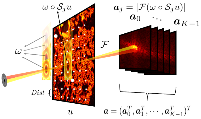
Fig. 1: Ptychographic phase retrieval (Far-field): A stack of amplitudes $\bm{a}_{j}=|\mathcal{F}(\omega\circ\mathcal{S}_{j}u)|$ is collected, with $\omega$ being the localized coherent probe, and $u$ being the image of interest (sample). The white dots represent the scanning lattice points, with $D$ denoting the sliding distance between centers of two adjacent frames.

In a ptychography experiment (Figure 1), a localized coherent X-ray probe (illumination) $\omega$ scans through an image (sample) $u$, while a 2D detector collects a sequence of phaseless intensities in the far field. Throughout the paper, we consider Ptycho-PR in a discrete setting as follows: A 2D image is expressed as $u\in\mathbb{C}^{n}$ with $\sqrt{n}\times\sqrt{n}$ pixels, $\omega\in\mathbb{C}^{\bar{m}}$ is a localized 2D probe with $\sqrt{\bar{m}}\times\sqrt{\bar{m}}$ pixels ($u$ and $\omega$ are both written as a vector by a lexicographical order), and  $\bm{a}_{j}\in\mathbb{R}_{+}^{\bar{m}}~{}\forall 0\leq j\leq J-1$ corresponds to a stack of phaseless measurements, collected with $\bm{a}_{j}=|\mathcal{F}(\omega\circ\mathcal{S}_{j}u)|.$ Operation $|\cdot|$ represents the element-wise absolute value of a vector, $\circ$ denotes the element-wise multiplication, $\mathcal{S}_{j}\in\mathbb{R}^{\bar{m}\times n}$ is a binary matrix that defines a small window with the index $j$ and size $\bar{m}$ over the entire image $u$, and $\mathcal{F}$ denotes the normalized discrete Fourier transformation. In practice, as the probe is almost never completely known, one has to solve a blind ptychographic phase retrieval (BP-PR) problem [21]:

(1) $${\text{BP-PR:\qquad To find ~{}}\omega\in\mathbb{C}^{\bar{m}}\text{~{}and~{}}u\in\mathbb{C}^{n},~{}~{}}s.t.~{}~{}|\mathcal{A}(\omega,u)|=\bm{a},$$

where bilinear operators $\mathcal{A}:\mathbb{C}^{\bar{m}}\times\mathbb{C}^{n}\rightarrow\mathbb{C}^{m}$ and $\mathcal{A}_{j}:\mathbb{C}^{\bar{m}}\times\mathbb{C}^{n}\rightarrow\mathbb{C}^{\bar{m}}~{}\forall 0\leq j\leq J-1$, are denoted as follows: $\mathcal{A}(\omega,u):=(\mathcal{A}_{0}^{T}(\omega,u),\mathcal{A}_{1}^{T}(\omega,u),\cdots,\mathcal{A}_{J-1}^{T}(\omega,u))^{T},$ $\mathcal{A}_{j}(\omega,u):=\mathcal{F}(\omega\circ\mathcal{S}_{j}u),$ and $\bm{a}:=(\bm{a}^{T}_{0},\bm{a}^{T}_{1},\cdots,\bm{a}^{T}_{J-1})^{T}\in\mathbb{R}^{m}_{+}.$

1.1 State-of-the-art algorithms

When the probe is exactly known, Ptycho-PR corresponds to a general phase retrieval (PR) problem. Multiple efficient algorithms have been designed during the last years to solve both general phase retrieval [27, 36], and non-blind (no probe retrieval) Ptycho-PR problems [35, 19, 41, 29, 34, 39, 30, 11, 43]. An early work by Chapman [9] to solve the blind problem used the Wigner-Distribution deconvolution method to retrieve the probe (zone-plate pupil). The more recent algorithms that focus on the blind Ptycho-PR problem (1) are described below.

1.1.1 Projection Algorithms

In the optics community, projection algorithms such as Alternating Projections (AP) are very popular for non-blind PR problems [27]. Some projection algorithms have also been applied to BP-PR problems, e.g. Douglas-Rachford (DR) algorithm by Thibault et al. [37], extended ptychographic engine (ePIE) by Maiden and Rodenburg [26], and relaxed averaged alternating reflections [25] based projection algorithm by Marchesini et al. [28]. Projection algorithms for PR involve a projection onto a nonconvex modulus constraint set, and therefore, their convergence studies are very challenging. Although some progress has been made for the general PR problem using projection algorithms  [20, 30, 10], the corresponding convergence for the blind problem is still unclear. Arguably, the most popular projection algorithms for BP-PR are ePIE and DR, described in detail below.

i) DR. Given an exit wave $\Psi:=(\Psi^{T}_{0},\Psi^{T}_{1},\cdots,\Psi_{J-1}^{T})^{T}\in\mathbb{C}^{m},$ with $\Psi_{j}:=\omega\circ\mathcal{S}_{j}u~{}\forall 0\leq j\leq J-1,$ one needs to find the exit wave $\Psi^{\star}$ that belongs to the intersection of two sets, i.e. $\Psi^{\star}\in\widehat{\mathscr{X}}_{1}\bigcap\widehat{\mathscr{X}}_{2},$ with

(2) $$\widehat{\mathscr{X}}_{1}:=\{\Psi:=(\Psi^{T}_{0},\Psi^{T}_{1},\cdots,\Psi_{J-1}^{T})^{T}\in\mathbb{C}^{m}:~{}|\mathcal{F}\Psi_{j}|=\bm{a}_{j}~{}\forall 0\leq j\leq J-1\},$$

$\widehat{\mathscr{X}}_{2}:=\{\Psi\in\mathbb{C}^{m}:~{}\exists\omega\in\mathbb{C}^{\bar{m}},u\in\mathbb{C}^{n},s.t.~{}~{}\omega\circ\mathcal{S}_{j}u=\Psi_{j}~{}\forall 0\leq j\leq J-1\}.$

The AP algorithm that determines this intersection needs to calculate the projections onto $\widehat{\mathscr{X}}_{1}$ and $\widehat{\mathscr{X}}_{2}$. Regarding the projection onto $\widehat{\mathscr{X}}_{1}$ as $\widehat{\mathcal{P}}_{1}(\Psi):=\arg\min_{\widehat{\Psi}\in\widehat{\mathscr{X}}_{1}}\|\widehat{\Psi}-\Psi\|^{2},$ with $\|\cdot\|$ denoting the $L^{2}$ norm in complex Euclidean space, one readily gets a closed form solution $\widehat{\mathcal{P}}_{1}(\Psi):=\big{(}(\widehat{\mathcal{P}}_{1}^{0}(\Psi))^{T},\cdots,(\widehat{\mathcal{P}}_{1}^{J-1}(\Psi))^{T}\big{)}^{T},$ with $\widehat{\mathcal{P}}_{1}^{j}(\Psi)=\mathcal{F}^{-1}(\bm{a}_{j}\circ\mathrm{sign}(\mathcal{F}\Psi_{j}))~{}0\leq j\leq J-1,$ where $\forall~{}z\in\mathbb{C}^{m},$ $(\mathrm{sign}(z))(t):=\mathrm{sign}(z(t))~{}\forall 0\leq t\leq m-1$. For the projection onto $\widehat{\mathscr{X}}_{2}$, given $\Psi^{k}$ as the solution in the $k^{\text{th}}$ iteration, one gets $\widehat{\mathcal{P}}_{2}(\Psi^{k}):=((\omega^{k+1}\circ\mathcal{S}_{0}u^{k+1})^{T},(\omega^{k+1}\circ\mathcal{S}_{1}u^{k+1})^{T},\cdots,(\omega^{k+1}\circ\mathcal{S}_{J-1}u^{k+1})^{T})^{T},$ where

(3) $$(\omega^{k+1},u^{k+1})=\arg\min\limits_{\omega,u}F(\omega,u,\Psi^{k}):=\tfrac{1}{2}{\textstyle\sum\nolimits_{j}}\|\Psi^{k}_{j}-\omega\circ\mathcal{S}_{j}u\|^{2},$$

with $\sum\nolimits_{j}$ being a simplified form of $\sum\nolimits_{j=0}^{J-1}.$ When solving (3) inexactly by alternating minimization (after $T$ steps) as

(4) $$\omega_{l+1}=\arg\min_{\omega}F(\omega,u_{l},\Psi^{k}),u_{l+1}=\arg\min_{u}F(\omega_{l+1},u,\Psi^{k})~{}\forall l=0,1,\cdots,T-1,$$

the DR algorithm for BP-PR can be formulated in two steps [37], as follows:

(1) Compute $\widehat{\Psi}^{k}$ by $\widehat{\Psi}^{k}_{j}=\omega^{k+1}\circ\mathcal{S}_{j}u^{k+1}$, where $(\omega^{k+1},u^{k+1})$ is solved by (4).

(2) Compute $\Psi^{k+1}$ by $\Psi^{k+1}=\Psi^{k}+\widehat{\mathcal{P}}_{1}(2\widehat{\Psi}^{k}-\Psi^{k})-\widehat{\Psi}^{k}$.

ii) ePIE. This iterative algorithm can be expressed as an AP method for BP-PR as follows: To find $\Psi^{\star}_{n_{k}}$ belonging to the intersection as

$$\Psi^{\star}_{n_{k}}\in\{|\mathcal{F}\Psi_{n_{k}}|=\bm{a}_{n_{k}}\}\cap\{\Psi_{n_{k}}:~{}\exists\omega\in\mathbb{C}^{\bar{m}},u\in\mathbb{C}^{n},~{}~{}s.t.~{}~{}\omega\circ\mathcal{S}_{n_{k}}u=\Psi_{n_{k}}\},$$

with a random frame index $n_{k}$. By first computing the projection $\psi^{k}_{n_{k}}$ by $\widehat{\mathcal{P}}_{1}^{n_{k}}(\psi^{k}_{n_{k}})$, and then updating $\omega^{k+1}$ and $u^{k+1}$ by the gradient descent algorithm (inexact projection), the ePIE algorithm [26] can be expressed by updating $\omega^{k+1}$ and $u^{k+1}$ in parallel as

$$\left\{\begin{split}&\omega^{k+1}=\omega^{k}-\tfrac{d_{2}}{\|\mathcal{S}_{n_{k}}(u^{k})^{*}\|^{2}_{\infty}}\mathcal{S}_{n_{k}}(u^{k})^{*}\circ(\Psi^{k}_{n_{k}}-\widehat{\mathcal{P}}_{1}^{n_{k}}(\Psi^{k}_{n_{k}}))\\ &u^{k+1}=u^{k}-\tfrac{d_{1}}{{\|\omega^{k}\|^{2}_{\infty}}}\mathcal{S}_{n_{k}}^{T}\left({(\omega^{k})^{*}}\circ(\Psi^{k}_{n_{k}}-\widehat{\mathcal{P}}_{1}^{n_{k}}(\Psi^{k}_{n_{k}}))\right),\end{split}\right.$$

with frame index $n_{k}\in\{0,1,\cdots,J-1\}$ generated randomly, and positive parameters $d_{1}$ and $d_{2}$, where $\omega^{k},u^{k}$ are the solutions in the $k^{\text{th}}$ iteration, $(\cdot)^{*}$ denotes the complex conjugate of a vector pointwise, and $\|\omega\|_{\infty}:=\max_{t}|\omega(t)|$.

1.1.2 Proximal Alternating Linearized Minimization

The proximal alternating linearized minimization (PALM) method [3] was applied to BP-PR in [21], which solved a least squares problem with a nonconvex constraint set as follows:

(5) $$\min\limits_{\omega,u,\Psi}F(\omega,u,\Psi)+\mathbb{I}_{\widehat{\mathscr{X}}_{1}}(\Psi),$$

with $F(\omega,u,\Psi)$ and $\widehat{\mathscr{X}}_{1}$ denoted in (3) and (2), respectively, and the indicator function $\mathbb{I}_{\widehat{\mathscr{X}}_{1}}$ denoted as: $\mathbb{I}_{\widehat{\mathscr{X}}_{1}}(\Psi)\!=\!0,~{}\text{if~{}}\Psi\in\widehat{\mathscr{X}}_{1},\text{otherwise~{}}\mathbb{I}_{\widehat{\mathscr{X}}_{1}}(\Psi)\!=\!+\infty.$ PALM [See [21], Algorithm 2.1] can be expressed in two steps:

(1) Compute $\omega^{k+1},u^{k+1}$ sequentially by alternating minimizing $F(\omega,u,\Psi^{k})$ by the gradient descent scheme as ePIE.

(2) Compute $\Psi^{k+1}$ by $\Psi^{k+1}=\widehat{\mathcal{P}}_{1}\big{(}\tfrac{1}{{1+\gamma}}({\widehat{\Psi}^{k+1}+\gamma\Psi^{k}})\big{)},$ with $\widehat{\Psi}^{k+1}_{j}:=\omega^{k+1}\circ S_{j}u^{k+1},$ and the positive parameter $\gamma$.

Under the assumption of boundedness of iterative sequences, the convergence of PALM to stationary points of (5) was proved [21]. The parallel version of PALM was also provided, presenting multiple similarities with ePIE. The main difference between them is that for ePIE, only the gradient of $F$ w.r.t. a randomly selected single frame is adopted to update $\omega$ and $u$ per outer loop, while for PALM, each block of $\omega$ and $u$ can be updated in parallel by employing the gradient w.r.t. all adjacent frames. Therefore, the parallel version of PALM is numerically more robust than ePIE.

1.2 Motivations and Contributions

Existing algorithms for BP-PR still have several limitations. The convergence speed of PALM [21] is not satisfactory (See the convergence curves in cyan in the first row of Figure 6). AP algorithms for BP-PR as DR [37] and ePIE [26] tend to be unstable: visible drifts of the probe happen during iterations of DR (See Figure 7 (a)), and the iterative sequence of ePIE could diverge if the measurements are few or noisy. In addition, the existing algorithms reviewed in section 1.1 for BP-PR were derived based on a least squares model that ignored the impact of experimental noise, e.g. Poisson noise.

The alternating direction method of multipliers (ADMM) [17, 42, 4] was adopted to solve non-blind PR problems in [41, 6], where it demonstrated fast convergence and robustness. However, it has never been applied to BP-PR problems (1). On the theoretical side, only the subsequence convergence of ADMM was proved for non-blind PR problems in [41], which relied on a relatively strong assumption of the convergence for the successive error of the multiplier.

In this paper we propose a more efficient method that employs the generalized form of ADMM [15, 47, 18, 13], a typical extension of standard ADMM. The main contributions of this paper are summarized below:

• We propose a nonlinear least squares model for BP-PR with constraints on the image and probe, driven by the maximum likelihood estimation of the Poisson noise. We also formulate a variant optimization model by incorporating the Fourier magnitudes of the probe to attenuate artifacts caused by the periodical lattices based scanning.

• We design fast generalized ADMMs to solve the proposed models, whose subproblems can be efficiently solved with comparatively few elementwise operations. With suitable stepsizes, we prove their convergence to stationary points for the proposed models under mild conditions.

• We conduct numerous experiments to show the convergence and efficiency of the proposed algorithms. Compared with the state of the art, the proposed algorithms present a significantly better convergence speed: their R-factor decreases faster, while producing higher quality images. When using additional information from the probe, the proposed algorithms also successfully attenuate artifacts from the periodical lattice based scanning. We report more than $10\times$ acceleration by using a non-optimized GPU implementation in Matlab, which demonstrates how the method can be trivially parallelized, showing great potential for large-scale problems.

The reminder of the paper is organized as follows: Section 2 gives the nonlinear least squares models for BP-PR, as well as the Lipschitz property. Fast generalized ADMMs are given in section 3 with convergence guarantees shown in section 4. Numerous experiments are conducted to verify the effectiveness of proposed algorithms in section 5. Section 6 summarizes this work.​​

2 Proposed Models

Instead of directly solving the quadratic multidimensional systems in (1), following [34] for non-blind Ptycho-PR, a nonlinear least squares model for BP-PR can be given as

$$\min\nolimits_{\omega\in\mathbb{C}^{\bar{m}},u\in\mathbb{C}^{n}}\tfrac{1}{2}\||\mathcal{A}(\omega,u)|-\bm{a}\|^{2}.$$

In order to deal with data contaminated by different types of noise, based on the maximum likelihood estimation (MLE), more general mappings [8] to measure the distance between the recovered intensity $g\in\mathbb{R}_{+}^{m}$ and the collected noisy intensity $f\in\mathbb{R}_{+}^{m}$, have been extensively studied for the PR problem:

(6) $$\left\{\begin{split}&\tfrac{1}{2}\|\sqrt{g}\!-\!\sqrt{f}\|^{2},\quad\qquad\quad\mbox{~{}Amplitude Gaussian Metric (AGM)~{} \cite[cite]{[\@@bibref{}{qian2014efficient,wen2012}{}{}]}}\\ &\tfrac{1}{2}\langle g\!-\!f\circ\log(g),\bm{1}_{m}\rangle,\phantom{..}\quad\mbox{Intensity Poisson Metric (IPM) \cite[cite]{[\@@bibref{}{thibault2012maximum,chang2016Total}{}{}]}}\\ &\tfrac{1}{2}\big{\|}g\!-\!f\big{\|}^{2},\phantom{.}\qquad\quad\qquad\enspace\mbox{~{}Intensity based Gaussian Metric (IGM)~{} \cite[cite]{[\@@bibref{}{qian2014efficient}{}{}]}}\\ &\!\!\tfrac{1}{2}\|\tfrac{g}{\sqrt{f+\varepsilon\mathbf{1}_{m}}}\!-\!\tfrac{f}{\sqrt{f+\varepsilon\mathbf{1}_{m}}}\|^{2},\phantom{-}\mbox{Weighted Intensity Gaussian Metric (wIGM)~{} \cite[cite]{[\@@bibref{}{qian2014efficient}{}{}]},}\end{split}\right.$$

where $\mathbf{1}_{m}\in\mathbb{R}^{m}$ represents a vector whose elements are all ones, $\sqrt{\cdot}$ and $\tfrac{~{}\cdot~{}}{~{}\cdot~{}}$ denote element-wise square root and division of a vector, respectively, $\varepsilon>0$ is the penalization factor, and $\langle\cdot,\cdot\rangle$ denotes the $L^{2}$ inner product in Euclidean space. IPM is derived from the MLE for Poisson noise, and AGM can be interpreted as a metric based on the variance-stabilizing transform for Poisson noise [28].

In this paper, we focus on Poisson noisy measurements, which are typical during photon-counting procedures in real experiments. However, the resulted objective functionals for BP-PR directly based on AGM and IPM in (6) are not Lipschitz differentiable, such that it is difficult to design first order splitting algorithms with convergence guarantee. Therefore, we consider the following two modified metrics with the penalization parameter $\varepsilon>0$ as follows:

(7) $$\!\mathcal{B}(g,f)\!=\!\left\{\begin{split}&\tfrac{1}{2}\|\sqrt{g+\varepsilon\mathbf{1}_{m}}\!-\!\sqrt{f+\varepsilon\mathbf{1}_{m}}\|^{2},\qquad\qquad\qquad\phantom{,.}\mbox{~{}Penalized-AGM (pAGM)}\\ &\tfrac{1}{2}\langle g+\varepsilon\mathbf{1}_{m}\!-\!(f+\varepsilon\mathbf{1}_{m})\circ\log(g+\varepsilon\mathbf{1}_{m}),\bm{1}_{m}\rangle,\phantom{..}\mbox{Penalized-IPM (pIPM) }\\ \end{split}\right.$$

with $\mathcal{B}(\cdot,\cdot):\mathbb{R}^{m}_{+}\times\mathbb{R}^{m}_{+}\rightarrow\mathbb{R}_{+}$. Consequently, a nonlinear optimization model for BP-PR is given as:

(8) $$\text{Model I:\qquad}\min\nolimits_{\omega\in\mathbb{C}^{\bar{m}},u\in\mathbb{C}^{n}}\mathcal{G}(\mathcal{A}(\omega,u)){+\mathbb{I}_{\mathscr{X}_{1}}(\omega)+\mathbb{I}_{\mathscr{X}_{2}}(u),}$$

with $\mathcal{G}(z):=\mathcal{B}(|z|^{2},f)$, where the amplitude constraints of the probe and image as [21, 28] are incorporated, where $\mathscr{X}_{1}:=\{\omega\in\mathbb{C}^{\bar{m}}:~{}\|\omega\|_{\infty}\leq C_{\omega}\}$ and $\mathscr{X}_{2}:=\{u\in\mathbb{C}^{n}:~{}\|u\|_{\infty}\leq C_{u}\}$ with two positive constants $C_{\omega},C_{u}$.

If the collected data is noise free, the minimizer to (8) exists if the solution set $\{(\omega,u)\in\mathscr{X}_{1}\times\mathscr{X}_{2}:|\mathcal{A}(\omega,u)|=\bm{a}\}\not=\emptyset$. For the data possibly contaminated by noise, the following proposition shows the existence of the minimizer to Model I.

Proposition 1.

Model I admits at least one minimizer.

It is standard to show the existence of a minimizer to Model I, and we omit the details.

The generalized derivative for complex-valued variables are adopted as in [21, 6] by separating the real and imaginary parts of the variables and operators defined in the complex space. Below we denote the Lipschitz property of the function $\mathcal{G}$ defined on $\mathbb{C}^{m}$.

Definition 1 (Lipschitz Property).

The function $\Phi:\mathbb{C}^{m}\rightarrow\mathbb{R}$ has the Lipschitz property in $\mathbb{C}^{m}$ with a Lipschitz constant $L$ if

• It is Lipschitz differentiable (its gradient is Lipschitz continuous), i.e.

  (9) $$\|\nabla\Phi(v_{1})-\nabla\Phi(v_{2})\|\leq L\|v_{1}-v_{2}\|~{}\forall v_{1},v_{2}\in\mathbb{C}^{m};$$

• It has the descent property as

  (10) $$\Phi(v_{2})-\Phi(v_{1})-\Re(\langle\nabla\Phi(v_{1}),v_{2}-v_{1}\rangle)\leq\tfrac{L}{2}\|v_{2}-v_{1}\|^{2}~{}\forall v_{1},v_{2}\in\mathbb{C}^{m}.$$

Following [1], letting $\Phi$ be smooth in $C^{1}$, the second relation (10) holds if it is Lipschitz differentiable as (9). It is well known that the Lipschitz property of the objective functional is of high importance to prove the convergence of first-order splitting algorithms for a nonconvex minimization problem [44, 3, 40, 22]. We show the Lipschitz property of $\mathcal{G}$ in the following lemma.

Lemma 2.1.

The function $\mathcal{G}(\cdot)$ has the Lipschitz property.

Proof.

The function $\mathcal{G}(z)$ with each metric in (7) is $C^{\infty}$ smooth, and we just need to show the Lipschitz continuity of its gradient. The corresponding first order derivatives are given below:

(11) $$\nabla\mathcal{G}(z)=\left\{\begin{split}&z-\tfrac{\sqrt{f+\varepsilon\bm{1}_{m}}}{\sqrt{|z|^{2}+\varepsilon\bm{1}_{m}}}\circ z~{}\text{for pAGM};\\ &z-\tfrac{f+\varepsilon\bm{1}_{m}}{|z|^{2}+\varepsilon\bm{1}_{m}}\circ z~{}\text{for pIPM}.\end{split}\right.$$

A basic estimate is given below:

(12) $$\|v_{1}\circ v_{2}\|\leq\|v_{1}\|_{\infty}\|v_{2}\|,~{}\forall~{}v_{1},v_{2}\in\mathbb{C}^{m}.$$

In order to prove the first property in (9), $\forall~{}v_{1},v_{2}\in\mathbb{C}^{m}$, by (11), we have

$$\begin{split}&\|\nabla\mathcal{G}(v_{2})-\nabla\mathcal{G}(v_{1})\|\leq\|v_{2}-v_{1}\|+\big{\|}\tfrac{\sqrt{f+\varepsilon\bm{1}_{m}}}{\sqrt{|v_{2}|^{2}+\varepsilon\bm{1}_{m}}}\circ v_{2}-\tfrac{\sqrt{f+\varepsilon\bm{1}_{m}}}{\sqrt{|v_{2}|^{2}+\varepsilon\bm{1}_{m}}}\circ v_{1}\big{\|}\\ &\hskip 142.26378pt+\big{\|}\tfrac{\sqrt{f+\varepsilon\bm{1}_{m}}}{\sqrt{|v_{2}|^{2}+\varepsilon\bm{1}_{m}}}\circ v_{1}-\tfrac{\sqrt{f+\varepsilon\bm{1}_{m}}}{\sqrt{|v_{1}|^{2}+\varepsilon\bm{1}_{m}}}\circ v_{1}\big{\|}\\ &\stackrel{{\scriptstyle\eqref{eq3}}}{{\leq}}(1+\big{\|}\tfrac{\sqrt{f+\varepsilon\bm{1}_{m}}}{\sqrt{|v_{2}|^{2}+\varepsilon\bm{1}_{m}}}\big{\|}_{\infty})\|v_{2}-v_{1}\|\\ &\hskip 28.45274pt+\big{\|}\sqrt{f+\varepsilon\bm{1}_{m}}\circ\tfrac{v_{1}\circ(|v_{1}|+|v_{2}|)}{\sqrt{|v_{1}|^{2}+\varepsilon}\sqrt{|v_{2}|^{2}+\varepsilon}(\sqrt{|v_{1}|^{2}+\varepsilon}+\sqrt{|v_{2}|^{2}+\varepsilon})}\big{\|}_{\infty}\big{\|}|v_{1}|-|v_{2}|\big{\|}\\ &\leq(1+\tfrac{2}{\sqrt{\varepsilon}}\|{\sqrt{f+\varepsilon\bm{1}_{m}}}\big{\|}_{\infty})\|v_{2}-v_{1}\|.\end{split}$$

Similarly, in the case of pIPM, we have

$$\|\nabla\mathcal{G}(v_{2})-\nabla\mathcal{G}(v_{1})\|\leq(1+\tfrac{2}{{\varepsilon}}\|{{f+\varepsilon\bm{1}_{m}}}\big{\|}_{\infty})\|v_{2}-v_{1}\|,$$

that completes the Lemma. ∎

For BP-PR (1), or Model I in the noise free case (without constraints), trivial solutions always exist, i.e. scaling, reflection or translation. Moreover, there exists nontrivial solutions, which possibly depends on the scanning geometry. Especially, with periodical-lattice based scanning, there exists evident structural artifacts in the recovered images [37]. Specifically, assuming that $(\omega,u)$ is a solution to (1) for the noiseless case, the nontrivial solution $(\hat{\omega},\hat{u})$ can be generated as $(\hat{\omega},\hat{u}):=(p_{1}\circ\omega,p_{2}\circ u)$ with two periodical functions $p_{1},p_{2}$ (not constants) satisfying $\mathcal{S}_{j_{1}}p_{2}=\mathcal{S}_{j_{2}}p_{2}\equiv\tfrac{\bm{1}_{\bar{m}}}{p_{1}}~{}\forall 0\leq j_{1},j_{2}\leq J-1,$ such that $p_{1}\circ\mathcal{S}_{j}p_{2}\equiv\bm{1}_{\bar{m}}.$ Readily, it can be seen how $(\hat{\omega},\hat{u})$ is a solution to (1), since

$$\hat{\omega}\circ\mathcal{S}_{j}\hat{u}=(p_{1}\circ\omega)\circ\mathcal{S}_{j}(p_{2}\circ u)=(p_{1}\circ\mathcal{S}_{j}p_{2})\circ(\omega\circ\mathcal{S}_{j}u)=\omega\circ\mathcal{S}_{j}u.$$

Due to the existence of nontrivial solutions to (1), the existing algorithms may get trapped into finding a solution with periodical structures (Figure 4 (b, k) and Figure 5 (b, k)), which completely breaks features of the image of interest. In order to deal with nontrivial ambiguities, non-periodical lattices based scanning can be considered experimentally to remove the periodicity of the scanning geometry, e.g. adding a small amount of random offsets to a set of square-lattice (or raster grid) [26], using a circular scan geometry [14] or Fermat spiral scan geometry [23]. However, in practice, square lattice or other periodical lattices based scanning are very popular for being straightforward and easy to implement, and we have to explore more a-priori information of the unknown probe to attenuate artifacts with the periodical scanning geometry.

In real experiments, the specimen can be simply removed to collect the diffraction pattern of the unknown probe in far-field. Hence, in the following optimization problem, we leverage the additional data $\bm{c}\in\mathbb{R}^{\bar{m}}_{+}$ to eliminate structural artifacts and further increase the reconstruction accuracy:

(13) $$\text{Model II:\qquad}\min\limits_{\omega\in\mathbb{C}^{\bar{m}},u\in\mathbb{C}^{n}}\mathcal{G}(\mathcal{A}(\omega,u)){+\mathbb{I}_{\mathscr{X}_{1}}(\omega)+\mathbb{I}_{\mathscr{X}_{2}}(u)}+\tau\widehat{\mathcal{G}}(\mathcal{F}\omega),$$

where $\tau$ is a positive parameter, the additional measurement $\bm{c}$ is the diffraction pattern (absolute value of Fourier transform of the probe) as $\bm{c}:=|\mathcal{F}u|$, and $\widehat{\mathcal{G}}(z):=\mathcal{B}(|z|^{2},\bm{c}^{2}),$ with $\bm{c}^{2}$ denoting the pointwise square of the vector $c$. For simplicity, assume that $\mathcal{G}$ and $\hat{\mathcal{G}}$ adopt the same metric. We remark that such information can be used as a constraint condition as in [28]. Similarly to Proposition 1, the existence of a minimizer to Model II can be readily derived.

3 Numerical Algorithms

The proposed models are non-convex and non-smooth, and they can be solved by a block coordinate descent method with proximal linear version [44], or PALM [3], equivalently. We conduct an experiment using PALM [3] for Model I. Equivalent results can be obtained using the block coordinate descent method, BCD [44], and the detailed iterative scheme can be found in Appendix A. The recovery results using PALM (BCD) are presented in Figure 2. By observing the recovery images in Figure 2 (b, c), obvious artifacts including the periodical artifacts and ringing artifacts of the edges can be observed. Moreover, one can readily see that PALM (BCD) for Model I converges very slow inferred from Figure 2 (d), since in order to make these iterative algorithms be stable, very small stepsizes are selected manually, which results in slow convergence speed.

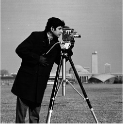
(a) Truth

(b) pAGM

(c) pIPM

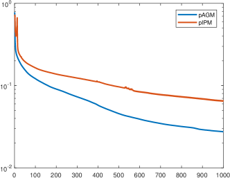
Fig. 2: Truth in (a), recovery images in (b, c) for Model I with pAGM and pIPM, and convergence histories (R-factor denotes the system residual) in (d) . All algorithms stop if $\mathrm{R-factor}^{k}\leq 1.0\times 10^{-6}$ or iteration number reaches $1000.$ $\mathrm{Dist}=16.$ Stepsizes $(\tau^{k}_{1},\tau^{k}_{2})=$ $(1.0\times 10^{-6},1.5\times 10^{-11})$, and $(5.0\times 10^{-6},1.0\times 10^{-6})$ for (b, c) respectively. Set $C_{u}=C_{\omega}=1.0\times 10^{8}.$ $\varepsilon=1.0\times 10^{-8}\times\|f\|_{\infty}.$

Alternatively, the generalized ADMM will be adopted to solve the proposed models, which permits bigger stepsizes by avoiding directly calculating the gradient of the objective functional such that fast convergence speed is gained. By introducing new variables, the proposed optimization problems are decoupled by operator-splitting of ADMM and the resulted subproblems can be easily solved. Additionally, proximal terms in the subproblems are introduced in order to guarantee the sufficient decrease of the augmented Lagrangian, such that the convergence of the proposed algorithm can be derived under mild conditions.

3.1 Generalized ADMM for Model I

An auxiliary variable $z=\mathcal{A}(\omega,u)\in\mathbb{C}^{m}$ is introduced such that an equivalent form of (8) is formulated as follows:

(14) $$\min\limits_{\omega,u,z}\mathcal{G}(z){+\mathbb{I}_{\mathscr{X}_{1}}(\omega)+\mathbb{I}_{\mathscr{X}_{2}}(u),}~{}~{}s.t.~{}~{}~{}z-\mathcal{A}(\omega,u)=0.$$

The corresponding augmented Lagrangian reads

(15) $$\begin{split}\!\!\!\!\Upsilon_{\beta}&(\omega,u,z,\Lambda):=\mathcal{G}(z){+\mathbb{I}_{\mathscr{X}_{1}}(\omega)+\mathbb{I}_{\mathscr{X}_{2}}(u)}+\Re(\langle z-\mathcal{A}(\omega,u),\Lambda\rangle)+\tfrac{\beta}{2}\|z-\mathcal{A}(\omega,u)\|^{2},\!\!\!\!\end{split}$$

with the multiplier $\Lambda\in\mathbb{C}^{m}$ and a positive parameter $\beta,$ where $\langle\cdot,\cdot\rangle$ corresponds to the $L^{2}$ inner product in complex Euclidean space and $\Re(\cdot)$ denotes the real part of a complex number. Consequently, instead of minimizing (8) directly, one seeks a saddle point of the following problem:

(16) $$\max_{\Lambda}\min\limits_{\omega,u,z}\Upsilon_{\beta}(\omega,u,z,\Lambda).$$

A natural scheme to solve the above saddle point problem is to split them, which consists of four-step iterations for the generalized ADMM (only the subproblems w.r.t. $\omega$ or $u$ have proximal terms), as follows:

(17) $$\left\{\begin{aligned} &\mbox{Step 1:\quad}\omega^{k+1}=\arg\min\limits_{\omega}{\Upsilon_{\beta}(\omega,u^{k},z^{k},\Lambda^{k})+\tfrac{\alpha_{1}}{2}\|\omega-\omega^{k}\|^{2}_{M_{1}^{k}}}\\ &\mbox{Step 2:}\quad u^{k+1}=\arg\min\limits_{u}{\Upsilon_{\beta}(\omega^{k+1},u,z^{k},\Lambda^{k})+\tfrac{\alpha_{2}}{2}\|u-u^{k}\|^{2}_{M_{2}^{k}}}\\ &\mbox{Step 3:\quad}z^{k+1}=\arg\min\limits_{z}\Upsilon_{\beta}(\omega^{k+1},u^{k+1},z,\Lambda^{k})\\ &\mbox{Step 4:\quad}\Lambda^{k+1}=\Lambda^{k}+\beta(z^{k+1}-\mathcal{A}(\omega^{k+1},u^{k+1})),\\ \end{aligned}\right.$$

with diagonal positive semidefinite matrices $M^{k}_{1}\in\mathbb{R}_{+}^{\bar{m}\times\bar{m}}$ and $M^{k}_{2}\in\mathbb{R}_{+}^{n\times n}$ (we call them preconditioning matrices as in [47]) and two penalization parameters $\alpha_{1},\alpha_{2}>0,$ where $\|\omega\|^{2}_{M_{1}^{k}}:=\langle M_{1}^{k}\omega,\omega\rangle$ and $\|u\|^{2}_{M_{2}^{k}}:=\langle M_{2}^{k}u,u\rangle$, given the approximated solution $(\omega^{k},u^{k},z^{k},\Lambda^{k})$ in the $k^{\text{th}}$ iteration. Here we remark that these two matrices $M_{1}^{k},M_{2}^{k}$ are assumed to be diagonal so that subproblems in Step 1 and Step 2 have closed form solutions. In practice, these two matrices are chosen heuristically, and a special strategy to guarantee the convergence will be specified in section 4 (See (43)).

3.1.1 Subproblems w.r.t. $\omega$ and $u$

First, we consider the subproblem in Step 1 of (17) w.r.t. the probe $\omega$:

$$\begin{split}&\omega^{k+1}=\arg\min\limits_{\omega\in\mathscr{X}_{1}}\tfrac{1}{2}\|\hat{z}^{k}-\mathcal{A}(\omega,u^{k})\|^{2}{+\tfrac{\alpha_{1}}{2\beta}\|\omega-\omega^{k}\|^{2}_{M_{1}^{k}}}\\ &=\arg\min\limits_{\omega\in\mathscr{X}_{1}}\tfrac{1}{2}{\sum\nolimits_{j}}\|\mathcal{F}^{-1}\hat{z}_{j}^{k}-\omega\circ\mathcal{S}_{j}u^{k}\|^{2}{+\tfrac{\alpha_{1}}{2\beta}\|\omega-\omega^{k}\|^{2}_{M_{1}^{k}}}\\ &=\arg\min\limits_{\omega\in\mathscr{X}_{1}}\sum\limits_{t=0}^{\bar{m}-1}\rho^{k}_{t}(\omega(t)),\text{~{}with~{}}\hat{z}^{k}:=z^{k}+\tfrac{\Lambda^{k}}{\beta},\end{split}$$

and $\rho^{k}_{t}(x):=\tfrac{1}{2}\sum_{j}|(\mathcal{F}^{-1}\hat{z}_{j}^{k})(t)-x\times(\mathcal{S}_{j}u^{k})(t)|^{2}{+\tfrac{\alpha_{1}}{2\beta}\mathrm{diag}(M_{1}^{k})(t)\times|x-\omega^{k}(t)|^{2}}~{}\forall x\in\mathbb{C},$ where $\omega(t)$ denotes the $t^{\text{th}}$ element of $\omega\forall 0\leq t\leq\bar{m}-1.$ Essentially this subproblem w.r.t. each element $\omega(t)$ is independent, such that one just needs to solve the following one-dimension constraint quadratic problem:

$$\omega^{k+1}(t)=\arg\min_{|x|\leq C_{\omega}}\rho_{t}^{k}(x)~{}0\leq t\leq\bar{m}-1.$$

The derivative of $\rho^{k}_{t}(x)$ is calculated as

$$\begin{split}&\quad\nabla\rho^{k}_{t}(x)\\ &=\sum\nolimits_{j}\big{(}x\times\left|\left(\mathcal{S}_{j}u^{k}\right)(t)\right|^{2}-(\mathcal{S}_{j}u^{k})^{*}(t)(\mathcal{F}^{-1}\hat{z}_{j}^{k})(t)\big{)}{+\tfrac{\alpha_{1}}{\beta}\mathrm{diag}(M_{1}^{k})(t)\times(x-\omega^{k}(t))}\\ &=x\times\big{(}\sum\nolimits_{j}\left|\left(\mathcal{S}_{j}u^{k}\right)(t)\right|^{2}+{\tfrac{\alpha_{1}}{\beta}\mathrm{diag}(M_{1}^{k})(t)}\big{)}-\sum\nolimits_{j}\left((\mathcal{S}_{j}u^{k})^{*}(t)(\mathcal{F}^{-1}\hat{z}_{j}^{k})(t)\right)\\ &\hskip 199.16928pt{-\tfrac{\alpha_{1}}{\beta}\mathrm{diag}(M_{1}^{k})(t)\omega^{k}(t)},\end{split}$$

where $\mathrm{diag}(M_{1}^{k})(t)$ denotes the $t^{\text{th}}$ element of $\mathrm{diag}(M_{1}^{k})$. Letting $M_{1}^{k}$ satisfy

(18) $$\min\nolimits_{t}\sum\nolimits_{j}\left|\left(\mathcal{S}_{j}u^{k}\right)(t)\right|^{2}+\tfrac{\alpha_{1}}{\beta}\mathrm{diag}(M_{1}^{k})(t)>0,$$

the close form solution of Step 1 is given as

(19) $$\omega^{k+1}=\mathrm{Proj}\Big{(}\tfrac{\beta\sum\nolimits_{j}(\mathcal{S}_{j}u^{k})^{*}\circ(\mathcal{F}^{-1}\hat{z}_{j}^{k}){+{\alpha_{1}}\mathrm{diag}(M_{1}^{k})\circ\omega^{k}}}{\beta\sum\nolimits_{j}\left|\mathcal{S}_{j}u^{k}\right|^{2}+{\alpha_{1}}\mathrm{diag}(M_{1}^{k})};C_{\omega}\Big{)},$$

with the projection operator onto $\mathscr{X}_{1}$ defined as $\mathrm{Proj}(\omega;C_{\omega}):=\min\{C_{\omega},|\omega|\}\circ\mathrm{sign}(\omega).$

Second, we consider the subproblem in Step 2 of (17) w.r.t. the variable $u$ as

$$u^{k+1}= \arg\min_{u\in\mathscr{X}_{2}}\tfrac{\beta}{2}\sum\nolimits_{j}\|\hat{z}_{j}^{k}\!-\!\mathcal{F}(\omega^{k+1}\circ\mathcal{S}_{j}u)\|^{2}{+{\alpha_{2}}\|u-u^{k}\|^{2}_{M_{2}^{k}}}$$

$$= \arg\min_{u}\tfrac{\beta}{2}\sum\nolimits_{j}\|\mathcal{S}_{j}^{T}\mathcal{F}^{-1}\hat{z}_{j}^{k}-(\mathcal{S}_{j}^{T}\omega^{k+1})\circ u\|^{2}{+{\alpha_{2}}\|u-u^{k}\|^{2}_{M_{2}^{k}}}.$$

Similarly to (19), letting $M_{2}^{k}$ satisfy

(20) $$\min\nolimits_{t}\sum\nolimits_{j}\left|\left(\mathcal{S}_{j}^{T}\omega^{k+1}\right)(t)\right|^{2}+\tfrac{\alpha_{2}}{\beta}\mathrm{diag}(M_{2}^{k})(t)>0,$$

we have

(21) $$u^{k+1}=\mathrm{Proj}\Big{(}\tfrac{\beta\sum_{j}\mathcal{S}_{j}^{T}((\omega^{k+1})^{*}\circ\mathcal{F}^{-1}\hat{z}_{j}^{k})+\alpha_{2}\mathrm{diag}(M_{2}^{k})\circ u^{k}}{\beta\sum_{j}(\mathcal{S}_{j}^{T}|\omega^{k+1}|^{2})+\alpha_{2}\mathrm{diag}(M_{2}^{k})};C_{u}\Big{)}.$$

3.1.2 Subproblem w.r.t. $z$

The subproblem w.r.t. the variable $z$ reads

(22) $$\begin{split}\!\!\!z^{k+1}\!=\arg\min\limits_{z}\mathcal{G}(z)+\tfrac{\beta}{2}\big{\|}z-\mathcal{A}(\omega^{k+1},u^{k+1})+\tfrac{\Lambda^{k}}{\beta}\big{\|}^{2}=\mathrm{Prox}^{\beta}_{\mathcal{G}}\big{(}\mathcal{A}(\omega^{k+1},u^{k+1})-\tfrac{\Lambda^{k}}{\beta}\big{)},\!\!\!\\ \end{split}$$

where the proximal operator [32] $\mathrm{Prox}_{\mathcal{G}}^{\beta}:\mathbb{C}^{m}\rightarrow\mathbb{C}^{m}$ is defined as:

$$\mathrm{Prox}_{\mathcal{G}}^{\beta}(z):=\arg\min_{\hat{z}}\mathcal{G}(\hat{z})+\tfrac{\beta}{2}\|\hat{z}-z\|^{2},$$

and it is simplified by $\mathrm{Prox}_{\mathcal{G}}(z)$ in the case of $\beta=1.$

For the case of pIPM, we have

$$z^{k+1}=\arg\min_{z}\tfrac{1}{2}\langle|z|^{2}+\varepsilon\mathbf{1}_{m}-(f+\varepsilon\mathbf{1}_{m})\circ\log(|z|^{2}+\varepsilon\mathbf{1}_{m}),\mathbf{1}_{m}\rangle+\tfrac{\beta}{2}\|z-z^{+}\|^{2},$$

with $z^{+}=\mathcal{A}(\omega^{k+1},u^{k+1})-\tfrac{\Lambda^{k}}{\beta}.$ The solution can be expressed as

(23) $$z^{k+1}=\rho^{\star}\circ\mathrm{sign}(z^{+}),$$

where

(24) $$\rho^{\star}(t)=\arg\min_{0\leq x\in\mathbb{R}}\tfrac{1}{2}x^{2}-(f(t)+\varepsilon)\log(x^{2}+\varepsilon)+\tfrac{\beta}{2}(x-|z^{+}(t)|)^{2}.$$

The first optimality condition of the above optimization problem without constraints yields a quartic equation, such that it is possible to compare the function values at all non-negative roots. The root with the minimal value is the exact solution to this optimization problem. However, the computation cost to calculate all roots of a quartic equation is still relatively high. Alternatively, the gradient projection scheme can be expressed as:

(25) $$x_{l+1}=\max\left\{0,x_{l}-\delta\big{(}(1+\beta-\tfrac{f(t)+\varepsilon}{|x_{l}|^{2}+\varepsilon})x_{l}-\beta z^{+}(t)\big{)}\right\},\forall~{}l=0,1,\ldots$$

with the stepsize $\delta>0,$ and $x_{0}:=|z^{k}(t)|.$

For the case of pAGM, similarly to the case of pIPM, the solution $z^{k+1}$ can be given by (23), and the iterative scheme for $\rho^{\star}(t)$ is given as:

(26) $$x_{l+1}=\max\left\{0,x_{l}-\delta\big{(}(1+\beta-\tfrac{\sqrt{f(t)+\varepsilon}}{\sqrt{|x_{l}|^{2}+\varepsilon}})x_{l}-\beta z^{+}(t)\big{)}\right\},\forall~{}l=0,1,\ldots$$

Based on the above calculations, the generalized ADMM for Model I is summarized in Algorithm 1.

Algorithm 1     Generalized ADMM for Model I in (8)

0:    Set $\omega^{0},u^{0},z^{0}=\mathcal{A}(\omega^{0},u^{0}),\Lambda^{0}=0,k:=0,$ maximum iteration number $Iter_{Max}$, and parameters $\beta$, $\alpha_{1}$ and $\alpha_{2}$.

0:    $u^{\star}:=u^{Iter_{Max}}$ and $\omega^{\star}:=\omega^{Iter_{Max}}.$

1:  for $k=0$ to $Iter_{Max}-1$ do

2:     Compute $\omega^{k+1}$ by (19) with $\hat{z}^{k}:=z^{k}+\tfrac{\Lambda^{k}}{\beta},$ where $M_{1}^{k}$ satisfies (18).

3:     Compute $u^{k+1}$ by (21), where $M_{2}^{k}$ satisfies (20).

4:     Compute $z^{k+1}$ by (22).

5:     Update the multiplier as Step 4 of (17).

6:  end for

3.2 Generalized ADMM for Model II

By introducing two auxiliary variables $z_{1}\in\mathbb{C}^{m}$ and $z_{2}\in\mathbb{C}^{\bar{m}}$, an equivalent form of (13) can be obtained as:

$$\begin{split}\min\limits_{\omega,u,z_{1},z_{2}}&\qquad\mathcal{G}(z_{1}){+\mathbb{I}_{\mathscr{X}_{1}}(\omega)+\mathbb{I}_{\mathscr{X}_{2}}(u)}+\tau\widehat{\mathcal{G}}(z_{2}),\\ s.t.~{}~{}&\qquad z_{1}-\mathcal{A}(\omega,u)=0,~{}z_{2}-\mathcal{F}\omega=0.\end{split}$$

The corresponding augmented Lagrangian reads

(27) $$\begin{split}&\widehat{\Upsilon}_{\beta_{1},\beta_{2}}(\omega,u,z_{1},z_{2},\Lambda_{1},\Lambda_{2}):=\mathcal{G}(z_{1}){+\mathbb{I}_{\mathscr{X}_{1}}(\omega)+\mathbb{I}_{\mathscr{X}_{2}}(u)}+\Re(\langle z_{1}-\mathcal{A}(\omega,u),\Lambda_{1}\rangle)\\ &\qquad\quad+\tfrac{\beta_{1}}{2}\|z_{1}-\mathcal{A}(\omega,u)\|^{2}+\tau\widehat{\mathcal{G}}(z_{2})+\Re(\langle z_{2}-\mathcal{F}\omega,\Lambda_{2}\rangle)+\tfrac{\beta_{2}}{2}\|z_{2}-\mathcal{F}\omega\|^{2},\end{split}$$

with two multipliers $\Lambda_{1}\in\mathbb{C}^{m},\Lambda_{2}\in\mathbb{C}^{\bar{m}}$ and positive parameters $\beta_{1}$ and $\beta_{2}.$ Consequently, one needs to solve a saddle point problem as follows:

$$\max_{\Lambda_{1},\Lambda_{2}}\min\limits_{\omega,u,z_{1},z_{2}}\widehat{\Upsilon}_{\beta_{1},\beta_{2}}(\omega,u,z_{1},z_{2},\Lambda_{1},\Lambda_{2}).$$

The generalized ADMM is also used to solve the above problem, and in the following discussion, we focus on the subproblems of ADMM. First, we consider the subproblem w.r.t. $\omega$:

$$\!\!\omega^{k+1}=\arg\min\limits_{\omega\in\mathscr{X}_{1}}\tfrac{\beta_{1}}{2}\big{\|}z^{k}_{1}+\tfrac{\Lambda^{k}_{1}}{\beta_{1}}-\mathcal{A}(\omega,u^{k})\big{\|}^{2}+\tfrac{\beta_{2}}{2}\big{\|}\mathcal{F}^{-1}(z^{k}_{2}+\tfrac{\Lambda^{k}_{2}}{\beta_{2}})-\omega\big{\|}^{2}+\tfrac{\bar{\alpha}_{1}}{2}\|\omega-\omega^{k}\|^{2}_{\bar{M}_{1}^{k}},\!\!$$

with the penalization parameter $\bar{\alpha}_{1}>0$ and the preconditioning matrix $\bar{M}_{1}^{k}.$ Similarly to (19), by computing the first-order derivative, one readily obtains the solution:

(28) $${{\omega}^{k+1}=\mathrm{Proj}\Big{(}\tfrac{\beta_{1}\sum\nolimits_{j}(\mathcal{S}_{j}u^{k})^{*}\circ(\mathcal{F}^{-1}\bar{z}^{k}_{1,j})+\beta_{2}\mathcal{F}^{-1}\bar{z}^{k}_{2}+\bar{\alpha}_{1}\bar{M}_{1}^{k}\omega^{k}}{\beta_{1}\sum\limits\nolimits_{j}\left|\mathcal{S}_{j}u^{k}\right|^{2}+\beta_{2}\bm{1}_{\bar{m}}+\bar{\alpha}_{1}\mathrm{diag}(\bar{M}_{1}^{k})};C_{\omega}\Big{)},}$$

with $\bar{z}_{l}^{k}=z_{l}^{k}+\tfrac{\Lambda^{k}_{l}}{\beta_{l}},~{}l=1,2$ and $\bar{z}_{1}^{k}=((\bar{z}_{1,0}^{k})^{T},(\bar{z}_{1,1}^{k})^{T},\cdots,(\bar{z}_{1,J-1}^{k})^{T})^{T}\in\mathbb{C}^{m}$ with $\bar{z}^{k}_{1,j}\in\mathbb{C}^{\bar{m}}~{}\forall 0\leq j\leq J-1.$

Next, we consider the subproblem w.r.t. $u$. According to (21), its solution is directly given below:

(29) $$\min_{t}\beta_{1}\sum_{j}(\mathcal{S}_{j}^{T}|\omega^{k+1}|^{2})(t)+\bar{\alpha}_{2}\mathrm{diag}(\bar{M}_{2}^{k})(t)>0,$$

(30) $$u^{k+1}=\mathrm{Proj}\Big{(}\tfrac{\beta_{1}\sum_{j}(\mathcal{S}_{j}^{T}((\omega^{k+1})^{*}\circ\mathcal{F}^{-1}\bar{z}_{1,j}^{k}))+\bar{\alpha}_{2}\bar{M}_{2}^{k}u^{k}}{{\beta_{1}\sum_{j}(\mathcal{S}_{j}^{T}|\omega^{k+1}|^{2})+\bar{\alpha}_{2}\mathrm{diag}(\bar{M}_{2}^{k})}};C_{u}\Big{)},$$

with the penalization parameter $\bar{\alpha}_{2}>0,$ and the preconditioning matrix $\bar{M}_{2}^{k}.$

Regarding the subproblems w.r.t. $z_{1}$ and $z_{2},$ their closed form solutions can be directly derived as follows:

(31) $$z_{1}^{k+1}=\mathrm{Prox}^{\beta_{1}}_{\mathcal{G}}\big{(}\mathcal{A}(\omega^{k+1},u^{k+1})-\tfrac{\Lambda_{1}^{k}}{\beta_{1}}\big{)},\text{~{}and~{}}z_{2}^{k+1}=\mathrm{Prox}_{\widehat{\mathcal{G}}}^{\beta_{2}/\tau}\big{(}\mathcal{F}\omega^{k+1}-\tfrac{\Lambda_{2}^{k}}{\beta_{2}}\big{)},$$

where the proximal operators can be solved similarly to (23).

The generalized ADMM for Model II is summarized in Algorithm 2.

Algorithm 2       Generalized ADMM for Model II in (13)

0:    Set $\omega^{0},u^{0},z_{1}^{0}=\mathcal{A}(\omega^{0},u^{0}),z_{2}^{0}=\mathcal{F}\omega^{0},\Lambda_{1}^{0}=0,\Lambda_{2}^{0}=0,k:=0,$ maximum iteration number $Iter_{Max}$, and parameters $\beta_{1},\beta_{2},\tau,$ $\bar{\alpha}_{1}$ and $\bar{\alpha}_{2}$.

0:    $u^{\star}:=u^{Iter_{Max}}$ and $\omega^{\star}:=\omega^{Iter_{Max}}.$

1:  for $k=0$ to $Iter_{Max}-1$ do

2:     Compute $\omega^{k+1}$ by (28) with $\bar{z}_{l}^{k}:=z_{l}^{k}+\tfrac{\Lambda_{l}^{k}}{\beta},l=1,2.$

3:     Compute $u^{k+1}$ by (30) where $\bar{M}_{2}^{k}$ satisfies (29).

4:     Compute $z_{1}^{k+1},z_{2}^{k+1}$ by (31).

5:     Update multipliers as

$$\begin{split}&\Lambda_{1}^{k+1}=\Lambda_{1}^{k}+\beta_{1}(z_{1}^{k+1}-\mathcal{A}(\omega^{k+1},u^{k+1})),\\ &\Lambda_{2}^{k+1}=\Lambda_{2}^{k}+\beta_{2}(z_{2}^{k+1}-\mathcal{F}\omega^{k+1}).\end{split}$$

6:  end for

Since $\mathcal{F}$ is an orthogonal operator, and the operator $\mathcal{A}$ is block-wise defined based on element-wise multiplications of the probe and image for Ptycho-PR, their subproblems w.r.t. $\omega$ and $u$ have closed form solutions. We remark that, for the $z-$subproblem, very few iterations are needed to guarantee the convergence of the entire ADMM in practice, due to the error-forgetting property [46].

4 Convergence Analysis

First, we briefly review the framework for the convergence analysis of an iterative algorithm for nonconvex optimization problems. Consider an optimization problem $\min_{v}\Phi(v),$ with the functional $\Phi$ being proper, lower semi-continuous, and bounded below. Let an iterative sequence $\{v^{k}\}_{k=0}^{\infty}$ be generated by some algorithm to solve the above minimization problem. In light of [1, 3, 22, 40, 24, 31, 45], in order to prove that the iterative sequence converges to stationary points of $\Phi$, the following three conditions should be satisfied:

i) Sufficient decrease condition as

(32) $$\Phi(v^{k})-\Phi(v^{k+1})\geq c_{1}\|v^{k+1}-v^{k}\|^{2},\phantom{..}\mbox{with a positive constant $c_{1}$.}$$

ii) Relative error condition as

(33) $$\|p^{k+1}\|\leq c_{2}\|v^{k+1}-v^{k}\|,\mbox{ with some $p^{k+1}\in\partial\Phi(v^{k+1})$, and a positive constant $c_{2}$.}$$

iii) Kurdyka-Łojasiewicz (KL) property [1].

The first two conditions can guarantee that each limiting point of the iterative sequence is a stationary point of $\Phi,$ which demonstrates the subsequence convergence. Furthermore, by the KL property of $\Phi$, the iterative sequence can be proved to be a Cauchy sequence and therefore convergence can be reached. Along this line, the convergence for ADMM was established for noncovex problems [22, 40, 24, 31, 45].

In this section we analyze the convergence of the proposed generalized ADMM algorithm for this nonconvex optimization problem with the bilinear constraint. The sufficient-overlap condition of iterative sequences $\{\omega^{k}\}$ and $\{u^{k}\}$, which will be assumed to be bounded below by a positive constant, the difficulty brought by the bilinear constraint can be overcome. Thanks to the Lipschitz property of pAGM/pIPM based $\mathcal{G}$ (in Lemma 2.1), and the KL property of the objective functional of the proposed models, we shall be able to prove the convergence of the proposed algorithms.

The following notation is used for the successive error of the iterative sequences:

(34) $$E_{\omega}^{k+1}:=\omega^{k+1}\!-\!\omega^{k},E_{u}^{k+1}:=u^{k+1}\!-\!u^{k},E_{z}^{k+1}:=z^{k+1}\!-\!z^{k},E_{\Lambda}^{k+1}:=\Lambda^{k+1}\!-\!\Lambda^{k}.$$

4.1 Convergence of Algorithm 1

We show the first order optimality conditions for subproblems of (17). Letting $X^{k}:=(\omega^{k},u^{k},z^{k},\Lambda^{k})$ be generated by Algorithm 1, the following relations hold:

(35) $$0\in{\omega}^{k+1}\circ{\sum\nolimits_{j}\left|\mathcal{S}_{j}u^{k}\right|^{2}}-{\sum\nolimits_{j}(\mathcal{S}_{j}u^{k})^{*}\circ\mathcal{F}^{-1}(z_{j}^{k}+\tfrac{1}{\beta}\Lambda_{j}^{k})}$$

$$\hskip 85.35826pt+\tfrac{1}{\beta}\partial\mathbb{I}_{\mathscr{X}_{1}}(\omega^{k+1})+\tfrac{\alpha_{1}}{\beta}\mathrm{diag}(M_{1}^{k})\circ E_{\omega}^{k+1};$$

(36) $$0\in u^{k+1}\circ\!\sum\nolimits_{j}\mathcal{S}_{j}^{T}|\omega^{k+1}|^{2}\!-\sum\nolimits_{j}\mathcal{S}_{j}^{T}((\omega^{k+1})^{*}\circ\mathcal{F}^{-1}(z_{j}^{k}\!+\tfrac{1}{\beta}\Lambda_{j}^{k}))$$

$$\hskip 85.35826pt+\tfrac{1}{\beta}\partial\mathbb{I}_{\mathscr{X}_{2}}(u^{k+1})+\tfrac{\alpha_{2}}{\beta}\mathrm{diag}(M_{2}^{k})\circ E_{u}^{k+1};$$

(37) $$0=\nabla\mathcal{G}(z^{k+1})+\beta(z^{k+1}-\mathcal{A}(\omega^{k+1},u^{k+1}))+\Lambda^{k}.$$

Using (37) and the Step 4 of (17), one can derive

(38) $$0=\nabla\mathcal{G}(z^{k+1})+\Lambda^{k+1},~{}\forall k\geq 0.$$

We first estimate the differences of the augmented Lagrangian between two successive iterations to show the sufficient decrease as in (32).

Lemma 4.1 (Sufficient decrease condition).

For all $k\geq 1,$ we have

(39) $$\begin{split}\!\Upsilon_{\beta}(X^{k})\!-\!\Upsilon_{\beta}(X^{k+1})&\geq\tfrac{\beta}{2}I^{k}_{u}\|E_{\omega}^{k+1}\|^{2}\!+\!\tfrac{\beta}{2}I^{k}_{\omega}\|E_{u}^{k+1}\|^{2}\!+\!(\tfrac{\beta\!-\!3L}{2}\!-\!\tfrac{L^{2}}{\beta})\|E_{z}^{k+1}\|^{2},\end{split}$$

where $I^{k}_{u}\in\mathbb{R}_{+}$ and $I^{k}_{\omega}\in\mathbb{R}_{+}$ are defined below:

(40) $$\left\{\begin{split}&I^{k}_{u}:=\min_{0\leq t_{1}\leq\bar{m}-1}\sum\nolimits_{j}|(\mathcal{S}_{j}u^{k})(t_{1})|^{2}{+\tfrac{2\alpha_{1}}{\beta}\mathrm{diag}(M_{1}^{k})(t_{1}),}\\ &I^{k}_{\omega}:=\min_{0\leq t_{2}\leq n-1}\sum\nolimits_{j}|(\mathcal{S}^{T}_{j}\omega^{k+1})(t_{2})|^{2}{+\tfrac{2\alpha_{2}}{\beta}\mathrm{diag}(M_{2}^{k})(t_{2}).}\end{split}\right.$$

The corresponding proof can be found in Appendix B. We show the boundedness of the iterative sequence $\{X^{k}\}$ in the following lemma:

Lemma 4.2.

(Boundedness) Letting $\beta>\tfrac{3+\sqrt{17}}{2}L$, the sequence $\{X^{k}\}$ generated by Algorithm 1 is bounded. Furthermore, the sequence of augmented Lagrangian $\{\Upsilon_{\beta}(X^{k})\}$ is bounded and non-increasing.

The proof can be found in Appendix C. In order to make sure that the decreasing quantity of the augmented Lagrangian is bounded below by $\|X^{k+1}-X^{k}\|^{2}$, we need the following assumption:

Assumption 1 (Sufficient-Overlap).

The sequences $\{I^{k}_{u}\}\subseteq\mathbb{R}_{+},\{I^{k}_{\omega}\}\subseteq\mathbb{R}_{+}$, defined in (40), are bounded below by two constants $C_{1}$ and $C_{2}$, respectively, i.e.

(41) $$\inf\nolimits_{k}I^{k}_{u}\geq C_{1}>0,\qquad\inf\nolimits_{k}I^{k}_{\omega}\geq C_{2}>0.$$

Remark 4.1.

We discuss the above assumption for standard ADMM by setting $M^{k}_{1}=0,M_{2}^{k}=0$ in Algorithm 1, since it can work well in practice (further details can be found in Section 5). Assuming that the iterative sequences $\{\omega^{k}\}$ and $\{u^{k}\}$ converge to the ground truth solutions $\omega^{\star}$ and $u^{\star}$ for (8), which are also assumed to be nonzeros, under Assumption 1, the following inequalities hold:

(42) $$\begin{split}\min_{0\leq t_{1}\leq\bar{m}-1}\sum\nolimits_{j}|(\mathcal{S}_{j}u^{\star})(t_{1})|^{2}\geq C_{1},\qquad\min_{0\leq t_{2}\leq n-1}\sum\nolimits_{j}|(\mathcal{S}^{T}_{j}\omega^{\star})(t_{2})|^{2}\geq C_{2},\end{split}$$

which is a necessary condition for Assumption 1. Equation (42) holds when the sample is scanned with a small enough sliding distance so that each scan position sufficiently overlaps with the next. There must exist a positive number $k_{0}\geq 0$, such that for all $k\geq k_{0}$ the iterative sequences $\{I_{u}^{k}\}_{k\geq k_{0}}$ and $\{I_{\omega}^{k}\}_{k\geq k_{0}}$ are bounded below by some strictly positive constants. That explains the reasonability of Assumption 1. In practice, in order to guarantee the convergence for Ptycho-PR, scanning with smaller enough sliding distances is always needed so that enough redundancy between measurements can be attained. However, such assumption for standard ADMM is difficult to verify.

Due to the introduction of the proximal terms, these matrices can also be given by the following strategy:

(43) $$\mathrm{diag}(M_{1}^{k})(t_{1})=\left\{\begin{split}&s_{1},\qquad\text{if~{}}h_{1}^{k}\leq s_{1}\\ &{r_{1}h_{1}^{k}},\quad\text{otherwise,}\end{split}\right.~{}~{}\mathrm{diag}(M_{2}^{k})(t_{2})=\left\{\begin{split}&s_{2},\qquad\text{if~{}}h_{2}^{k}\leq s_{2}\\ &r_{2}{h_{2}^{k}},\quad\text{otherwise,}\end{split}\right.$$

where $h_{1}^{k}:=\big{\|}\sum\nolimits_{j}|(\mathcal{S}_{j}u^{k})|^{2}\big{\|}_{\infty},$ $h_{2}^{k}:=\big{\|}\sum\nolimits_{j}|(\mathcal{S}^{T}_{j}\omega^{k+1})|^{2}\big{\|}_{\infty},$ $s_{1},s_{2}$ are positive safeguard parameters, and $r_{1},r_{2}$ are positive constants. One readily knows that Assumption 1 holds with $C_{j}=\tfrac{2s_{j}\alpha_{j}}{\beta}\min\left\{1,r_{j}\right\}>0,j=1,2$ in (41). This strategy also guarantees that (18) and (20) hold, and the sequences of these two preconditioning matrices are bounded due to the boundednesses of $\{\omega^{k}\}$ and $\{u^{k}\}$.

The relative error condition, similarly to (33), is derived in the following lemma:

Lemma 4.3 (Relative error condition).

By letting $\beta>\tfrac{3+\sqrt{17}}{2}L$ and letting $\{\mathrm{diag}(M_{1}^{k})\},\{\mathrm{diag}(M_{2}^{k})\}$ be bounded, we have:

$${\mathrm{dist}(0,\partial\Upsilon_{\beta}(X^{k+1}))}\leq C_{3}\|X^{k+1}-X^{k}\|~{}\forall k\geq 0,$$

with a positive constant $C_{3}$.

The corresponding proof can be found in Appendix D. At this point, the convergence of Algorithm 1 can be derived in the following theorem:

Theorem 1.

Under Assumption 1 and $\beta>4L$, and letting $\{\mathrm{diag}(M_{1}^{k})\},$ $\{\mathrm{diag}(M_{2}^{k})\}$ be bounded, the iterative sequence $\{X^{k}\}$ generated by Algorithm 1 converges to a stationary point $X^{\star}$ of the augmented Lagrangian $\Upsilon_{\beta}$ in (15) for Model I in (8) with wIGM, i.e. $\lim_{k\rightarrow+\infty}X^{k}=X^{\star},\mbox{with~{}}{0\in\partial\Upsilon_{\beta}(X^{\star})}.$

The proof can be found in Appendix E. We remark that Assumption 1 can be verified when setting the preconditioning matrices as in (43), as well as the boundedness of the sequences of preconditioning matrices. Therefore, with suitable stepsizes and careful selection of the preconditioning matrices, one can derive the convergence of the proposed algorithms for Model I.

4.2 Convergence of Algorithm 2

Similarly to Assumption 1:

Assumption 2 (Sufficient-Overlap).

There exists a constant $\widehat{C}_{1}$ independent of $k$, such that $I_{\omega}^{k}$ defined in (40) is bounded below, i.e. $I^{k}_{\omega}\geq\widehat{C}_{1}>0.$

Based on the above two assumptions, we list the theorem below without proof, since it directly follows the proof of Theorem 1.

Theorem 2.

Under Assumptions 2, and letting $\{\mathrm{diag}(\bar{M}_{1}^{k})\},$ $\{\mathrm{diag}(\bar{M}_{2}^{k})\}$ be bounded, the iterative sequence generated by Algorithm 2 converges to a stationary point of the augmented Lagrangian $\widehat{\Upsilon}_{\beta_{1},\beta_{2}}$ in (27), provided that the parameters $\beta_{1},\beta_{2}$ are sufficiently large.

In order to derive the convergence of Algorithm 2, only the positive lower bound of $I_{\omega}^{k}$ is assumed. Hence, the convergence analysis of Algorithm 2 needs weaker conditions, compared to Algorithm 1. For the convergence guarantee of Algorithm 2, the boundedness of $I_{\omega}^{k}$ can be verified after the careful selection of the preconditioning matrix $\bar{M}_{2}^{k}$, similarly to (43).

5 Numerical Experiments

In the following experiments we consider that the probe scans the image of interest with periodical boundary condition on square, hexagonal or random lattices. The random lattice is generated based on the square lattice with additional random offsets within one pixel. The ground truth image and probe employed in this experiments can be found in Figure 4 (a) and Figure 13.

In order to evaluate performances of different algorithms, we introduce two criteria. First, the R-factor for Algorithms 1 and 2, defined as:

$$\text{R-factor}^{k}:=\tfrac{\sum\nolimits_{j}\big{\|}|\mathcal{A}_{j}(\omega^{k},u^{k})|-\sqrt{f_{j}}\big{\|}_{1}}{\|\sqrt{f}\|_{1}}.\!$$

If the R-factor of the iteration solutions of Algorithm 1 or 2 tends to zero as $k\rightarrow\infty$ for the noiseless case, they converge to global minimizers of the proposed models, which are also the stationary points. Therefore, in the case of noiseless data, R-factors can be used to verify the convergence. Secondly, the SNR (Signal-to-Noise Ratio) of $u^{k}$ is also employed, denoted as:

$$\mathrm{SNR}(u^{k},u_{g})=-10\log_{10}{\sum\limits_{t=0}^{n-1}|\zeta^{*}u^{k}(t+T^{*})-u_{g}(t)|^{2}}/{\|\zeta^{*}u^{k}\|^{2}},$$

with the ground truth image $u_{g}$, where the error is computed up to the translation $T^{*}$, phase shift and scaling factor $\zeta^{*}$ determined by

$$(\zeta^{*},T^{*}):=\arg\min\limits_{\zeta\in\mathbb{C},T\in\mathbb{Z}}\sum_{t}|\zeta u^{k}(t+T)-u_{g}(t)|^{2}.$$

Similarly, we can denote the $\mathrm{SNR}(\omega^{k},\omega_{g})$ for the probe, with $\omega_{g}$ being the ground truth. We also consider measurements contaminated by Poisson noise. In order to simulate different peak values, a factor $\eta>0$ is introduced [7] on the image, such that the Poisson noise corrupts the clean intensity as $f(t)\stackrel{{\scriptstyle\mathrm{i.d.d.}}}{{\sim}}\mathrm{Poisson}((\bm{a}^{\eta})^{2}(t))$, where $\bm{a}^{\eta}:=|\mathcal{A}(\omega_{g},\eta u_{g})|$ with ground truth $\omega_{g}$ and $u_{g}.$ One readily knows that noise level gets higher if $\eta$ gets smaller. For the noisy measurements, $\mathrm{SNR}_{intensity}$ [6] is used to measure the noise level, which is denoted below:

$$\mathrm{SNR}_{intensity}:=-10\log_{10}{\|f-(\bm{a}^{\eta})^{2}}\|^{2}/{\|(\bm{a}^{\eta})^{2}\|^{2}}.$$

In the following tests, we set $u^{0}=\bm{1}_{n}$ and $\omega^{0}=\tfrac{1}{J}\mathcal{F}^{-1}(\sum_{j}\sqrt{f_{j}})$, where the initial guess of the probe has zero phase for Algorithm 1-2. The parameters $C_{\omega},$ $C_{u}$ need to be sufficiently large, and we employ $C_{\omega}=C_{u}=1.0\times 10^{8}$ for the constraint sets in Models I and II. The same initial values of $u$ and $\omega$ are used for other compared algorithms. Other variables including auxiliary variables and multipliers are initialized as in the initialization stage in Algorithms 1-2. The parameters for the proposed algorithms are problem-dependent, which will be specified for different experiments. The codes are implemented in Matlab.

We remark that no obvious acceleration of the proposed algorithms can be observed when using more inner iterations for the subproblems of $z^{k}$ in Algorithm 1 and $z^{k}_{1},z_{2}^{k}$ in Algorithm 2. Due to the page limit, we do not report further details. Therefore, to reduce the overall computation cost, only one inner iteration is adopted.

5.1 Performance of Algorithm 1

We show the performance of Algorithm 1 with pAGM ($\varepsilon=1.0\times 10^{-8}\times\|f\|_{\infty}$), and then compare it with the state-of-the-art algorithms: DR [37], ePIE [26] and PALM [21]. The comparison algorithms are tuned and executed with the parameters that maximize their performance.

5.1.1 Comparison with DR, ePIE and PALM

We conduct experiments in the case of both noiseless and noisy measurements.

i) Noiseless case. We conduct the experiments with two different sliding distances $D=24,16$. Two different scanning lattices including square and random lattices are considered. We show the performances of Algorithm 1 in the following two cases: the standard ADMM with $M_{1}^{k}=M_{2}^{k}=0$ (referred below as ADMM) and the generalized version (43) with two additional proximal terms (ADMM-Prox), with $r_{1}=1.0\times 10^{-6},r_{2}=1.0\times 10^{-3},s_{1}=s_{2}=1.0\times 10^{-6}$, and $\alpha_{1}=\alpha_{2}=\beta$. First of all, in order to verify the sufficient-overlap condition, we plot the histories of $I^{k}_{u}$ and $I_{\omega}^{k}$ in Figure 3 ($D=24$). One readily knows that they quickly become stable, without approaching infinity or zero. Remarkably, without the proximal terms, the iterative sequences $\{I^{k}_{u}\}$ and $\{I_{\omega}^{k}\}$ by the standard ADMM also quickly tend to non-zero values. With the additional proximal terms, the sequences of ADMM-Prox get stable faster than those of the standard ADMM.

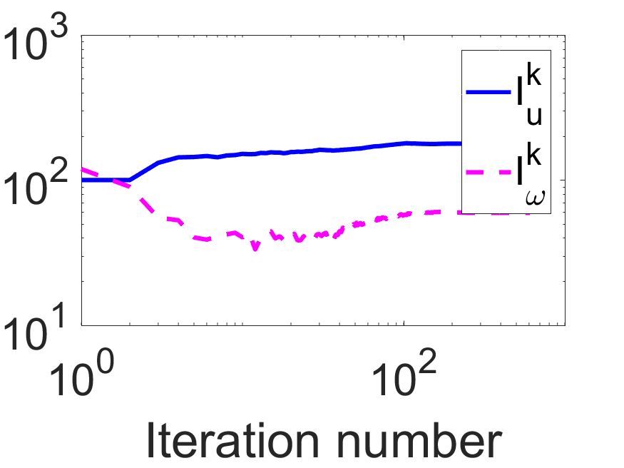
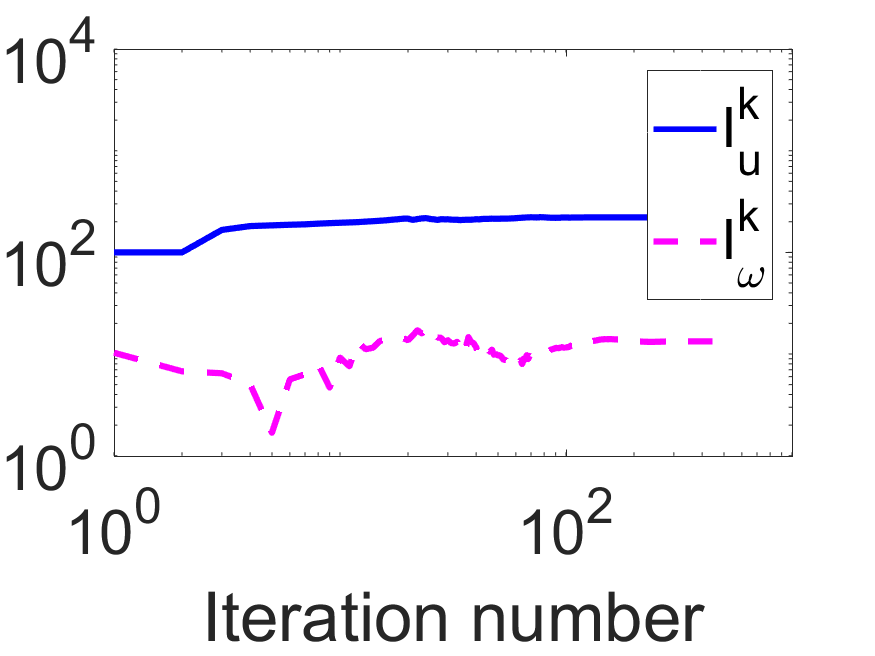
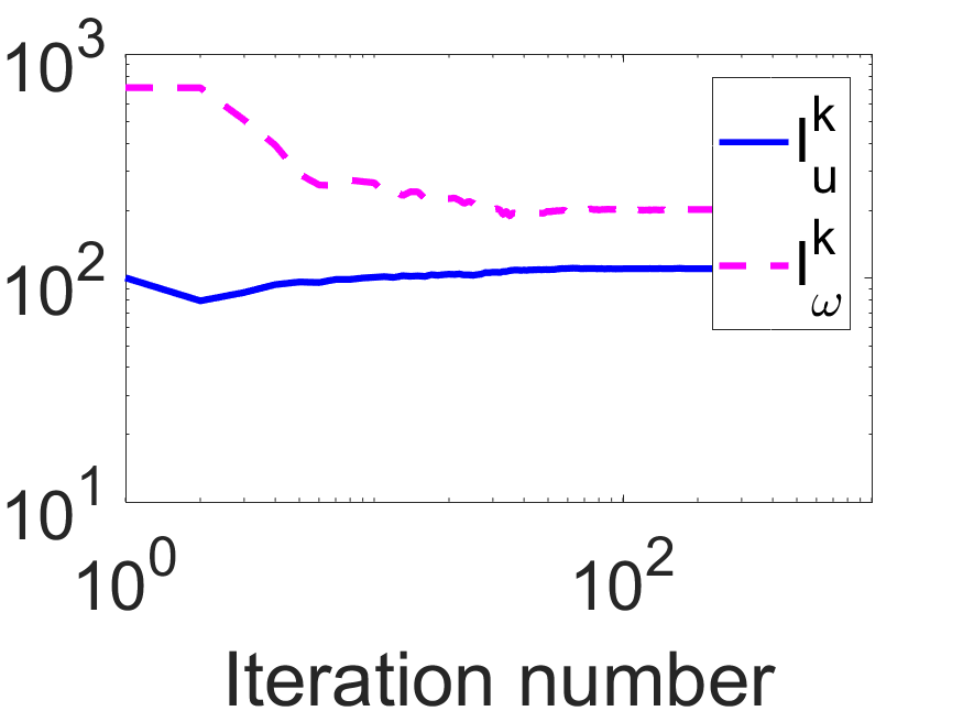
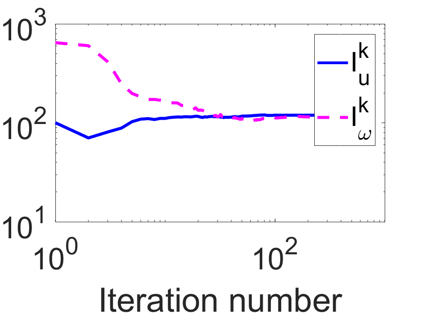
Fig. 3: Histories of $I_{u}^{k}$ and $I_{\omega}^{k}$ for ADMM (a, b) and ADMM-Prox (c, d) scanning on square-lattice (a, c) and random-lattice (b, d). $D=24$.

(a) Truth

(b) DR [37]

(c) PALM [21]

(d) ADMM

(e) ADMM-Prox

(f) DR [37]

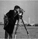
(g) PALM [21]

(h) ADMM

(i) ADMM-Prox

(j) ePIE [26]

(k) DR [37]

(l) PALM [21]

(m) ADMM

(n) ADMM-Prox

(o) ePIE [26]

(p) DR [37]

(q) PALM [21]

(r) ADMM

(s) ADMM-Prox

Fig. 4: Results of recovered images and probes by ePIE [26], DR [37], PALM [21] and ADMM (Algorithm 1) from left to right. D=24 ($m=6.25n$) in the 1st-2nd rows; D=16 ($m=16n$) in 3rd-4th rows. Scanning on square-lattice in 1st and 3rd rows and random-lattice in 2nd and 4th rows. (a): Ground truth for the image and probe with resolutions $n=256\times 256$ and $\bar{m}=64\times 64$ respectively.

(a) Truth

(b) DR [37]

(c) ​​PALM​[21]​​

(d) ADMM

(e) ADMM-Prox

(f) DR [37]

(g) PALM [21]

(h) ADMM

(i) ADMM-Prox

(j) ePIE [26]

(k) DR [37]

(l) PALM [21]

(m) ADMM

(n) ADMM-Prox

(o) ePIE [26]

(p) DR [37]

(q) PALM [21]

(r) ADMM

(s) ADMM-Prox

Fig. 5: Zoom-in views of the recovered images of Figure 4. D=24 in the 1st-2nd rows; D=16 in 3rd-4th rows. Scanning on square-lattice in 1st and 3rd rows and random-lattice in 2nd, 4th rows.

The results of the recovered images and probes are shown in Figure 4, and their corresponding zoom-in views in Figure 5. The recovery results demonstrate how ePIE and PALM are more sensitive to the number of measurements. With $D=24$, ePIE fails due to blow-up of its iterative solutions. The recovered images using PALM (Figure 4 (c, g), and its zoom-in Figure 5 (c, g)) present obvious stripe structures and ringing artifacts. With fewer number of measurements (or larger sliding distances), DR and Algorithm 1 work better than ePIE and PALM. In the first and third rows of Figures 4 and 5 (square-lattice scanning), periodical structural artifacts can be seen in all compared reconstructions. In the case of DR, such artifacts are specially severe. In the case of ADMM, ADMM-Prox, PALM and ePIE, those artifacts can be attenuated with $D=16$ (Figure 4 and 5 third row). The results from Figures 4 and 5 (first row) demonstrate how both ADMM and ADMM-Prox can still attenuate these artifacts with fewer number of measurements ($D=24$). In the case of random-lattice scanning (Figure 4 and 5, fourth row), all algorithms produce higher quality reconstructions. However, it can be noted in Figure 5 (zoom-in views) how ADMM, ADMM-Prox and DR can recover much sharper edges than ePIE and PALM.

The convergence analysis is presented in Figure 6. The R-factor in the case of ADMM and ADMM-Prox decreases faster than with the other compared algorithms w.r.t. the number of iterations. Furthermore, within one thousand iterations, the proposed algorithms reach the given tolerance. Those results experimentally demonstrate the convergence of the proposed algorithms, which is consistent with the previous convergence analysis. Specifically, inferred from the first row of Figure 6, ADMM and ADMM-Prox converge the fastest among all the compared algorithms: neither ePIE, PALM nor DR reach the desired tolerance within one thousand iterations. Due to the property of fast convergence of ADMM and ADMM-Prox, the SNRs of recovered images and probes are much higher than those by other algorithms. Execution times for the compared algorithms can be found in Table 1. Due to the additional update of the multipliers, the single step complexity of ADMM and ADMM-Prox is slightly higher than the compared algorithms. Because the proposed ADMM algorithms require fewer iterations, they achieve considerable lower execution times compared with DR, ePIE and PALM. ADMM and ADMM-Prox are 1.7 and 2 times faster, on average, for square- and random-lattice scanning, respectively.

The recovery images of ADMM-Prox with a careful selection of the preconditioning matrices have higher quality than those of standard ADMM: about 0.6 and 2.0 dB increase of SNRs from the images in Figure 6 (e, g) is gained. For the random-lattice scanning, they have very similar performances. In the following results, we run proposed algorithms simply setting the preconditioning matrices to zeros. Note that ADMM-Prox require more parameters to be tuned to gain the best performance but ADMM produces comparable results by tuning a single parameter.

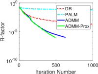
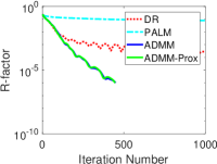
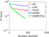
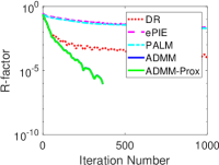
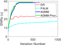
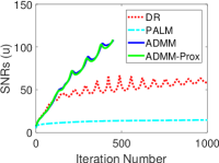
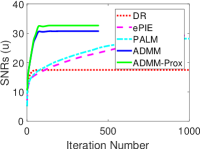
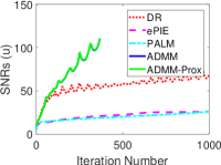
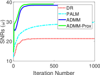
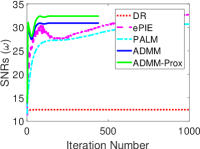
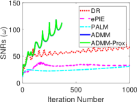
Fig. 6: Convergence histories of R-factor, SNRs of images and probes from up to down, respectively by ePIE [26], DR [37], PALM [21] and ADMM (Algorithm 1). D=24 in the 1st-2nd columns; D=16 in 3rd-4th columns. Scanning on square-lattice in 1st and 3rd columns and random-lattice in 2nd and 4th columns. All compared algorithms stop if $\mathrm{R-factor}^{k}\leq 1.0\times 10^{-6}$ or iteration number reaches $1000.$

Table 1: Runtimes of all compared algorithms. The format of the data “$\cdot/\cdot(\cdot)$” denotes “Elapsed time (in seconds)/Number of iterations (elapsed time per iteration)”. “-/-” means that the iterative solutions blow up. Note that the iteration number of ePIE means the number of cycles.

Cases		DR	ePIE	PALM	ADMM	ADMM-Prox
Square-lattice	D=24	170/1000(0.17)	-/-	115/1000(0.12)	93/633(0.15)	72/492(0.15)
	D=16	218/1000(0.22)	200/1000(0.20)	168/1000(0.17)	124/444(0.28)	124/444(0.28)
Random-lattice	D=24	150/1000(0.15)	-/-	108/1000(0.11)	65/452(0.14)	65/449(0.14)
	D=16	219/1000(0.22)	200/1000(0.20)	169/1000(0.17)	102/368(0.28)	102/368(0.28)

ii) Noisy case. Poisson noisy measurements are considered with peak levels $\eta=0.1$ and $1$, $D=16$, and random-lattice scanning. $\mathrm{SNR}_{intensity}=38.33,58.23$ for $\eta=0.1,1$ respectively. Since the iterative solutions of ePIE blow up, we only show results for ADMM, ADMM-Prox, DR and PALM. The reconstruction results can be found in Figure 7.

One should notice the obvious drift existing in the probe by DR in Figure 7 (a), with peak level $\eta=0.1$. For this reason, the quality of the recovered images of DR is the lowest among all compared algorithms, since DR does not have fixed points for an inconsistent feasibility problem [2]. At this noise level, ADMM and PALM can produce visually acceptable results. When the noise gets weak (peak level $\eta=1$) all algorithms can achieve high quality reconstructions, Figure 7 (second row). The zoom-in views of this experiment are presented in Figure 8. In this view we can see how the proposed ADMM algorithm, Figure 8 (c), presents much weaker ringing artifacts compared to PALM and DR, Figure 8 (a, b). At peak level $\eta=1,$ the recovered image from ADMM is nearly artifact-free, Figure 8 (g), while the results by the other two algorithms contain evident ringing artifacts, Figure 8 (e, f).

Convergence histories for this experiment can be found in Figure 9. The results of Figure 9 (a, c) demonstrate how DR is not stable with strong noise ($\eta=0.1$). The R-factors of ADMM are smaller than those obtained by PALM and DR, and the SNRs of the recovery results of ADMM are also higher than those obtained by PALM, which is consistent with the results shown in Figures 7 and 8. In summary, ADMM and PALM are more stable than DR and ePIE, and ADMM can recover images with higher quality than all the other compared algorithms.

DR [37]                    PALM [21]                           ADMM

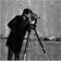
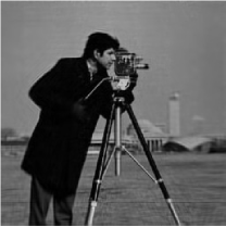
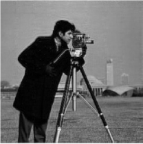
Fig. 7: Results of DR [37], PALM [21] and ADMM (Algorithm 1) with random-lattice scanning for Poisson noisy data. Peak level $\eta=0.1$ (top), $\eta=1$ (bottom). $\beta=0.5,0.2$ for Algorithm 1 with $\eta=0.1,1$, respectively. All compared algorithms stop when the iteration number reaches $Iter_{Max}=300$.

(a) DR [37]

(b) PALM[21]

(c) ADMM

(d) Truth

(e) DR [37]

(f) PALM[21]

(g) ADMM

Fig. 8: Zoom-in views of Figure 7 with random-lattice scanning. (d): zoom-in views of ground truth. (a, c), (e, g) are generated by magnifying Figure 7 (a, c), (d, f), respectively. (a, c) with $\eta=0.1$; (e, g) with $\eta=1.$

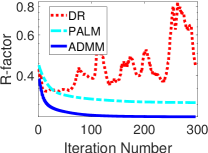
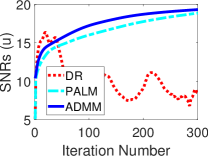
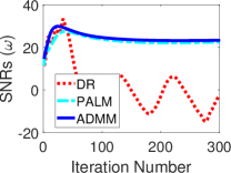
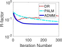
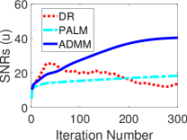
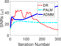
Fig. 9: Convergence histories (random-lattice scanning) of DR [37], PALM [21] and ADMM (Algorithm 1). Histories for R-factor, SNRs for the image and probe from left to right, respectively. $D=16$. Peak level $\eta=0.1$ (top), $\eta=1$ (bottom).

5.1.2 Different metrics

We show the performance of Algorithm 1 with four different metrics: pAGM, pIPM, IGM and wIGM (the latter two are defined in (6)). We conduct these experiments with $D=16$ and random-lattice scanning.

First, noiseless measurements are considered, with convergence histories shown in Figure 10. Within the first 50 iterations, R-factors with four different metrics decrease with almost the same speed. As the iterations go on, Algorithm 1 with IGM converges the slowest, and it is further accelerated with the weighted norm in wIGM. Algorithm 1 with pAGM/pIPM converges faster than when using the other two metrics.

We also consider the noisy measurements. Convergence histories for measurements contaminated by Poisson noise with $\eta=1$ are shown in Figure 10 (second row). It can be seen in Figure 10 (d) how ADMM with IGM converges at the slowest speed. When using pAGM or pIPM the convergence speed is slightly improved. Figure 10 (e, f) shows how the SNRs of the recovered results with pIPM are higher than those with the other metrics, since pIPM derives from the MLE for Poisson noise.

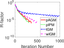
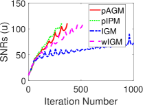
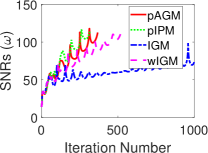
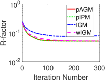
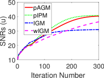
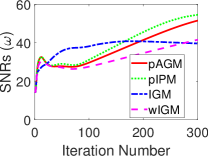
Fig. 10: Convergence histories for Algorithm 1 scanning on random-lattice with different metrics. Histories for R-factor (left), SNRs of the image (center) and probe (right). $D=16$. Noiseless data (top row) and Poisson noisy data with peak level $\eta=1$ (bottom row). For the noiseless data: stopping condition as $\mathrm{R-factor}^{k}\leq 1.0\times 10^{-6}$ or iteration number reaches $Iter_{Max}=1000;$ $\beta=0.04,0.1,0.04$ for pAGM, pIPM and IGM, respectively, and $\varepsilon=\beta=0.1$ for wIGM. For the noisy data: stopping condition as iteration number reaches $Iter_{Max}=300;$ $\beta=0.2,0.3,100,1$ for pAGM, pIPM, IGM and wIGM, respectively, and $\varepsilon=10$ for wIGM.

In summary, when dealing with noiseless measurements, pAGM or pIPM based metrics are recommended in order to gain faster convergence speed. For Poisson noisy data, pIPM should be used instead, in order to obtain higher quality reconstruction results. Due to the existence of noise, the recovered images seem blurry, which can be further improved by considering sparse prior information as in [6]. This study will be considered as future work for this research

5.2 Performance of Algorithm 2

In this section only noiseless data is considered, and experiments are performed with periodical scanning on square and hexagonal lattices. The reconstruction results of Algorithm 2 can be found in Figure 11, and its converge histories are reported in Figure 12.

With additional prior information of the probe, Algorithm 2 reconstructs images with higher SNRs, Figure 11 (b, d), in contrast with the results of Figure 11 (a, c) by Algorithm 1. We can see how Algorithm 2 is able to completely remove the structural artifacts. Figure 12 (a) shows how the R-factors of Algorithm 2 decrease faster compared with those from Algorithm 1, and fewer iterations are needed to reach the given tolerance. It is important to note that, as shown in Figure 12 (b, c), the SNRs of the reconstructed images and probes are greatly increased, which demonstrates the advantage of incorporating the prior information of the probe to the proposed algorithm.

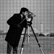
(a) ALG1

(b) ALG2

(c) ALG1

(d) ALG2

Fig. 11: Performance of ALG1 (Algorithm 1) in (a,c) and ALG2 (Algorithm 2) in (b, d). (a, b) with square-lattice, and (c, d) with hexagonal-lattice. Algorithm 2 with AGM stops if $\mathrm{R-factor}^{k}\leq 1.0\times 10^{-6}$ or if the iteration number reaches $Iter_{Max}=1000.$ $\tau=10,\beta_{1}=0.04,\beta_{2}=0.4$ for Algorithm 2.

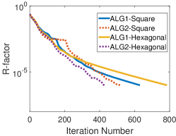
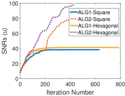
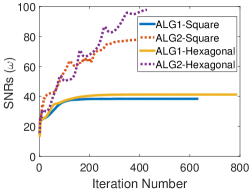
Fig. 12: Convergence histories of ALG1 (Algorithm 1) and ALG2 (Algorithm 2). Histories for R-factor (left), SNRs for the image (center) and probe (right).

5.3 GPU Acceleration

We conduct this experiment using Algorithm 1 with different $D\in\{12,8,6,4,3\}$ to produce large-scale data, since the number of measurements $m$ satisfies $m\approx\tfrac{n}{D^{2}}.$ Table 2 reports the corresponding execution times and GPU speedup ratios (SR) as $SR:={t_{CPU}}/{t_{GPU}}$. The GPU speedup ratios range between $12\sim 17$. Considering that the GPU Matlab implementation has not been optimized, the proposed algorithm shows great potential for large-scale BP-PR problems. The number of iterations ($IterNum$) to reach the given tolerance are about $300\sim 340$ with different $D$, which demonstrates that the convergence speed is not sensitive to the number of measurements for a large-scale problem. Although it is convenient to produce more measurements experimentally, with our algorithms, using fewer number of measurements can save memory and reduce the computation cost. One can also observe the computation cost for CPU (or GPU) is almost linear w.r.t. the number of measurements $m$, which is consistent with the runtime complexity of Algorithm 1 as about $O(m(\log_{2}\bar{m}+\tfrac{n}{\bar{m}})\times IterNum)$.

Table 2: Performances of Algorithm 1 on GPU v.s. CPU. $IterNum$ denotes the iteration number to reach the given tolerance, $t_{CPU}$ and $t_{GPU}$ denote the elapsed time in seconds for CPU and GPU, respectively. SR denotes the speedup ratio. Algorithm 1 stops if the R-factor is less than $1\times 10^{-5}$ or if the maximum iteration number reaches $1000$. The code runs on a desktop with CPU (Intel I7-4820K, 64GB RAM) and GPU (Nvidia TITAN-X with 12 GB GDDR5X) in single precision mode. The GPU version is directly implemented using the build-in functions of Matlab.

$D$	12	8	6	4	3
${m}$	$64^{2}\times 441$	$64^{2}\times 1024$	$64^{2}\times 1764$	$64^{2}\times 4096$	$64^{2}\times 7225$
$IterNum$	297	332	296	334	336
$t_{CPU}$ (s)	46.9	97.1	188.1	373.4	773.7
$t_{GPU}$ (s)	4.0	7.8	10.9	26.4	46.1
SR	11.7	12.4	17.2	14.1	16.8

5.4 Extensive tests: different probe and images

In order to test the robustness of proposed algorithms, we conduct more experiments on a different probe (non-circularly symmetric) with its absolute value shown in Figure 13 (c). Two other images shown in Figure 13 (a)-(b) are considered with scanning on square-lattice and random-lattice. The convergence curves of the R-factor, SNRs of recovered images and probes are reported in Figure 14, where one can readily see that the R-factors by proposed algorithms decrease faster, and the recovery results have better quality (bigger SNRs). Especially the test reported in the first column of Figure 14 shows that ADMM-Prox, with the help of additional proximal terms, becomes more stable and faster compared with standard ADMM.

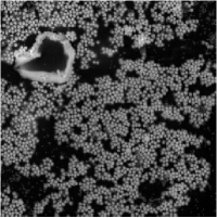
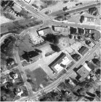
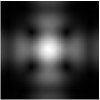
Fig. 13: Two testing images ($256\times 256$ pixels): A complex-valued image with the absolute value in (a), and a real-valued image in (b); A non-circularly symmetric probe in (c) with $64\times 64$ pixels (only show the absolute value)

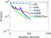
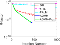
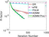
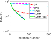
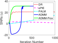
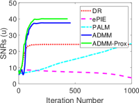
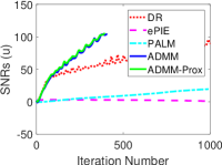
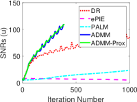
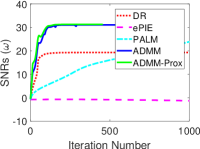
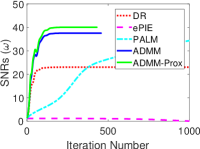
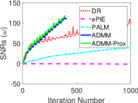
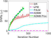
Fig. 14: Convergence histories of R-factor, SNRs of images and probes from up to down, respectively by ePIE [26], DR [37], PALM [21] and ADMM (Algorithm 1), with $D=24$ and scanning on square-lattice in 1st and 2nd columns and random-lattice in 3rd and 4th columns. All compared algorithms stop if $\mathrm{R-factor}^{k}\leq 1.0\times 10^{-6}$ or iteration number reaches $1000.$ Results for the complex-valued image (Figure 13 (a)) are put in the 1st, 3rd columns, and for the real-valued image (Figure 13(b)) in other columns.

6 Conclusions

In this paper we propose different nonlinear optimization models with and without prior information of the probe for the blind phase retrieval ptychography problem. Efficient generalized ADMMs are designed to solve the proposed models, and numerous numerical experiments demonstrate the superior performance of the proposed algorithms in both speed and reconstruction quality compared with the state-of-the-art algorithms. Especially, the performance on GPU reported in this paper have motivated the development of a high performance C++ multi-GPU implementation of the ADMM algorithm proposed in this paper. The multi-GPU implementation of ADMM was reported [16] to process more than 3 million measured samples per second on a single GPU, and it has already been installed and being used on the microscopes of the Advanced Light Source (ALS), at Lawrence Berkeley National Laboratory for real-time analysis [12] and partial coherence analysis [5].

Appendix A PALM or BCD for Model I in (8)

Iterative scheme for PALM or BCD in the $(k+1)^{\text{th}}$ iteration is given below:

$$\left\{\begin{split}&\omega^{k+1}=\arg\min_{\omega}\mathbb{I}_{\mathscr{X}_{1}}(\omega)+\tfrac{1}{2\tau^{k}_{1}}\|\omega-(\omega^{k}-\tau^{k}_{1}\nabla_{\omega}\mathcal{G}(\mathcal{A}(\omega^{k},u^{k})))\|^{2}\\ &u^{k+1}=\arg\min_{u}\mathbb{I}_{\mathscr{X}_{2}}(u)+\tfrac{1}{2\tau^{k}_{2}}\|u-(u^{k}-\tau^{k}_{2}\nabla_{u}\mathcal{G}(\mathcal{A}(\omega^{k+1},u^{k})))\|^{2},\end{split}\right.$$

with stepsizes $\tau^{k}_{1},\tau^{k}_{2}$, where

$$\begin{split}&\nabla_{\omega}\mathcal{G}(\mathcal{A}(\omega,u))=\sum_{j}(\mathcal{S}_{j}u^{*})\circ\mathcal{F}^{*}\big{(}\nabla_{z_{j}}\mathcal{G}(\mathcal{A}(\omega,u))\big{)},\\ &\nabla_{u}\mathcal{G}(\mathcal{A}(\omega,u))=\sum_{j}\mathcal{S}^{T}_{j}\Big{(}\omega^{*}\circ\mathcal{F}^{*}\big{(}\nabla_{z_{j}}\mathcal{G}(\mathcal{A}(\omega,u))\big{)}\Big{)},\end{split}$$

and $\nabla_{z}\mathcal{G}(z)$ is shown in (11).

Appendix B Proof of Lemma 4.1

We need the following estimate:

(44) $$\|v\|^{2}-\|w\|^{2}=\|v-w\|^{2}+2\Re(\langle w,v-w\rangle)~{}\forall v,w\in\mathbb{C}^{m}.$$

Denoting $\mathcal{Q}_{1}(\omega,u,z):=\mathcal{Q}(\omega,u,z)+\mathbb{I}_{\mathscr{X}_{1}}(\omega)+\tfrac{\alpha_{1}}{2\beta}\|\omega-\omega_{0}\|_{M_{1}}^{2}$ and $\mathcal{Q}_{2}(\omega,u,z):=\mathcal{Q}(\omega,u,z)+\mathbb{I}_{\mathscr{X}_{2}}(u)+\tfrac{\alpha_{2}}{2\beta}\|u-u_{0}\|^{2}_{M_{2}}$ with $\mathcal{Q}(\omega,u,z):=\tfrac{1}{2}\|\mathcal{A}(\omega,u)-z\|^{2},$ and two positive definite matrices $M_{1}$ and $M_{2}$, a basic estimate can be given below:

Letting $\omega^{\star}:=\arg\min_{\omega}\mathcal{Q}_{1}(\omega,u,z)$ and $u^{\star}:=\arg\min_{u}\mathcal{Q}_{2}(\omega,u,z)$,

(45) $$\mathcal{Q}(\omega_{0},u,z)-\mathcal{Q}(\omega^{\star},u,z){\geq}\tfrac{1}{2}\|\mathcal{A}(\omega_{0}-\omega^{\star},u)\|^{2}{+\tfrac{\alpha_{1}}{\beta}\|\omega^{\star}-\omega_{0}\|^{2}_{M_{1}},}$$

(46) $$\mathcal{Q}(\omega,u_{0},z)-\mathcal{Q}(\omega,u^{\star},z){\geq}\tfrac{1}{2}\|\mathcal{A}(\omega,u_{0}-u^{\star})\|^{2}{+\tfrac{\alpha_{2}}{\beta}\|u^{\star}-u_{0}\|^{2}_{M_{2}},}$$

for all $\omega_{0}\in\mathscr{X}_{1}$ and $u_{0}\in\mathscr{X}_{2},$ which can be easily derived by calculating the G$\mathrm{\hat{a}}$teaux derivative, (44), $\mathcal{A}(\omega,u)$ being bilinear and two constraint sets $\mathscr{X}_{1},\mathscr{X}_{2}$ being convex.

Proof.

First, we consider the subproblem in Step 1 of (17) as

(47) $$\begin{split}&\Upsilon_{\beta}(X^{k})-\Upsilon_{\beta}(\omega^{k+1},u^{k},z^{k},\Lambda^{k})=\stackrel{{\scriptstyle\eqref{eq13-1}}}{{\geq}}\tfrac{\beta}{2}\|\mathcal{A}(E_{\omega}^{k+1},u^{k})\|^{2}{+{\alpha_{1}}\|E^{k+1}_{\omega}\|^{2}_{M^{k}_{1}}}\\ &=\tfrac{\beta}{2}\sum\nolimits_{j}\|E_{\omega}^{k+1}\circ\mathcal{S}_{j}u^{k}\|^{2}{+{\alpha_{1}}\|E^{k+1}_{\omega}\|^{2}_{M^{k}_{1}}}\\ &=\tfrac{\beta}{2}\big{\langle}|E_{\omega}^{k+1}|^{2},\sum\nolimits_{j}|\mathcal{S}_{j}u^{k}|^{2}\big{\rangle}{+{\alpha_{1}}\|E^{k+1}_{\omega}\|^{2}_{M^{k}_{1}}}\geq\tfrac{\beta}{2}I_{u}^{k}\|E_{\omega}^{k+1}\|^{2}.\end{split}$$

For the subproblem in Step 2 of (17), similarly, we have

(48) $$\Upsilon_{\beta}(\omega^{k+1},u^{k},z^{k},\Lambda^{k})\!-\!\Upsilon_{\beta}(\omega^{k+1},u^{k+1},z^{k},\Lambda^{k})\geq\tfrac{\beta}{2}I_{\omega}^{k}\|E_{u}^{k+1}\|^{2}.$$

For the subproblem in Step 3 of (17), by (44) and (37), we have

$$\begin{split}&\Upsilon_{\beta}(\omega^{k+1},u^{k+1},z^{k},\Lambda^{k})-\Upsilon_{\beta}(\omega^{k+1},u^{k+1},z^{k+1},\Lambda^{k})\\ &=\mathcal{G}(z^{k})-\mathcal{G}(z^{k+1})+\tfrac{\beta}{2}\|E_{z}^{k+1}\|^{2}+\Re(\langle\nabla\mathcal{G}(z^{k+1}),E_{z}^{k+1}\rangle).\\ \end{split}$$

Then, using the Lemma 2.1, and Cauchy’s inequality as $\Re(\langle z_{1},z_{2}\rangle)\geq-\tfrac{L}{2}\|z_{1}\|^{2}-\tfrac{1}{2L}\|z_{2}\|^{2}$ $\forall$ $z_{1},$ $z_{2}$ $\in\mathbb{C}^{m},$ one readily has

(49) $$\begin{split}&\Upsilon_{\beta}(\omega^{k+1},u^{k+1},z^{k},\Lambda^{k})-\Upsilon_{\beta}(\omega^{k+1},u^{k+1},z^{k+1},\Lambda^{k})\\ \geq&\tfrac{\beta-2L}{2}\|E_{z}^{k+1}\|^{2}-\tfrac{1}{2L}\|\nabla\mathcal{G}(z^{k+1})-\nabla\mathcal{G}(z^{k})\|^{2}\geq\tfrac{\beta-3L}{2}\|E_{z}^{k+1}\|^{2}.\end{split}$$

Then we need to estimate the following relation as $\Upsilon_{\beta}(\omega^{k+1},u^{k+1},z^{k+1},\Lambda^{k})\!-\!\Upsilon_{\beta}(X^{k+1})\!\!$ $=-\tfrac{1}{\beta}\|E_{\Lambda}^{k+1}\|^{2},$ that yields the following inequality by (38) and Lemma 2.1

(50) $$\begin{split}&\!\Upsilon_{\beta}(\omega^{k+1},u^{k+1},z^{k+1},\Lambda^{k})\!-\!\Upsilon_{\beta}(\omega^{k+1},u^{k+1},z^{k+1},\Lambda^{k+1})\!\geq\!\!-\tfrac{L^{2}}{\beta}\|E_{z}^{k+1}\|^{2}.\end{split}$$

Finally, summing up (47) and (50) gives the desired lemma. ∎

Appendix C Proof of Lemma 4.2

Proof.

One can readily prove the nonincrease of the augmented Lagrangian with sufficiently large $\beta>\tfrac{3+\sqrt{17}}{2}L$ by Lemma 4.1. On the other hand,

$$\begin{split}&\quad\Upsilon(X^{k+1})\\ &\stackrel{{\scriptstyle\eqref{eqOptC-3-2}}}{{=}}\mathcal{G}(z^{k+1})-\Re(\langle z^{k+1}-\mathcal{A}(\omega^{k+1},u^{k+1}),\nabla\mathcal{G}(z^{k+1})\rangle)+\tfrac{\beta}{2}\|z^{k+1}-\mathcal{A}(\omega^{k+1},u^{k+1})\|^{2}\\ &\stackrel{{\scriptstyle\eqref{eqLipDescent}}}{{\geq}}\tfrac{\beta-L}{2}\|z^{k+1}-\mathcal{A}(\omega^{k+1},u^{k+1})\|^{2}+\mathcal{G}(\mathcal{A}(\omega^{k+1},u^{k+1})).\end{split}$$

Therefore, due to the boundedness of $\omega^{k}$ and $u^{k}$, the sequence $\{z^{k}\}$ is also bounded.

By (38), the boundedness of $\{z^{k}\}$, and $C^{\infty}$ smooth of $\mathcal{G}$, $\{\Lambda^{k}\}$ is also bounded. Therefore $\{X^{k}\}$ is bounded. As a result, the augmented Lagrangian is bounded as well, which completes this lemma. ∎

Appendix D Proof of Lemma 4.3

Proof.

We first estimate the upper bound of the partial derivative w.r.t. to $\omega$. By (35), there exists a variable $\bar{\omega}^{k+1}$ defined as

(51) $$\bar{\omega}^{k+1}:=-{\omega}^{k+1}\circ{\sum\nolimits_{j}\left|\mathcal{S}_{j}u^{k}\right|^{2}}+{\sum\nolimits_{j}(\mathcal{S}_{j}u^{k})^{*}\circ\mathcal{F}^{-1}(z_{j}^{k}+\tfrac{1}{\beta}\Lambda_{j}^{k})}-\tfrac{\alpha_{1}}{\beta}\mathrm{diag}(M_{1}^{k})\circ E_{\omega}^{k+1},$$

such that $\bar{\omega}^{k+1}\in\tfrac{1}{\beta}\partial\mathbb{I}_{\mathscr{X}_{1}}(\omega^{k+1}).$ Immediately,

$$\bar{\omega}^{k+1}+{\omega}^{k+1}\circ{\sum\nolimits_{j}\left|\mathcal{S}_{j}u^{k+1}\right|^{2}}\!-\!{\sum\nolimits_{j}(\mathcal{S}_{j}u^{k+1})^{*}\circ\mathcal{F}^{-1}\hat{z}_{j}^{k+1}}\in\tfrac{1}{\beta}\partial_{\omega}\Upsilon_{\beta}(X^{k+1}).$$

Hence we need to estimate the bound of the left hand side term of the above equation. Readily we have

(52) $$\begin{split}&{\mathrm{dist}(0,\partial_{\omega}\Upsilon_{\beta}(X^{k+1}))\!\leq\!\beta\Big{\|}\bar{\omega}^{k+1}+{\omega}^{k+1}\circ{\sum\nolimits_{j}\left|\mathcal{S}_{j}u^{k+1}\right|^{2}}\!-\!{\sum\nolimits_{j}(\mathcal{S}_{j}u^{k+1})^{*}\circ\mathcal{F}^{-1}\hat{z}_{j}^{k+1}}\Big{\|}}\\ &\stackrel{{\scriptstyle\eqref{eqOptC-1-1}}}{{\leq}}{{\alpha_{1}}\|\mathrm{diag}(M_{1}^{k})\circ E_{\omega}^{k+1}\|}+\beta\Big{\|}{\omega}^{k+1}\circ{\sum\nolimits_{j}\left|\mathcal{S}_{j}u^{k+1}\right|^{2}}\!-\!{\omega}^{k+1}\circ{\sum\nolimits_{j}\left|\mathcal{S}_{j}u^{k}\right|^{2}}\Big{\|}\!\\ &\qquad~{}~{}~{}+\beta\Big{\|}{\sum\nolimits_{j}(\mathcal{S}_{j}u^{k+1})^{*}\circ\mathcal{F}^{-1}\hat{z}_{j}^{k+1}}-{\sum\nolimits_{j}(\mathcal{S}_{j}u^{k})^{*}\circ\mathcal{F}^{-1}\hat{z}_{j}^{k}}\Big{\|}\\ &\!\leq\!{{\alpha_{1}}\|\mathrm{diag}(M_{1}^{k})\|_{\infty}\|E_{\omega}^{k+1}\|}+\beta\|{\omega}^{k+1}\|_{\infty}\big{\|}\sum\nolimits_{j}\mathcal{S}_{j}(|u^{k+1}|^{2}\!-\!|u^{k}|^{2})\big{\|}\!\\ \!&\!+\!\beta\Big{\|}{\sum\nolimits_{j}(\mathcal{S}_{j}E_{u}^{k+1})^{*}\circ\mathcal{F}^{-1}\hat{z}_{j}^{k}}\Big{\|}\!+\beta\Big{\|}{\sum\nolimits_{j}(\mathcal{S}_{j}u^{k+1})^{*}\circ\mathcal{F}^{-1}(z_{j}^{k+1}-z_{j}^{k}+\tfrac{1}{\beta}\Lambda_{j}^{k+1}-\tfrac{1}{\beta}\Lambda_{j}^{k})}\Big{\|},\!\!\end{split}$$

where the first two terms of last inequality are derived by (12). Then we will estimate three terms in the last inequality of (52) one by one. For the first term of the last inequality for (52), we have

(53) $$\begin{split}&\!\!\big{\|}\sum\nolimits_{j}\mathcal{S}_{j}(|u^{k+1}|^{2}-|u^{k}|^{2})\big{\|}\leq\sqrt{\rho(\mathcal{S})}\big{\|}|u^{k+1}|^{2}-|u^{k}|^{2}\big{\|}\\ &\!\!\!\!\stackrel{{\scriptstyle\eqref{eq3}}}{{\leq}}\!\sqrt{\rho(\mathcal{S})}\big{(}\|u^{k+1}\|_{\infty}\!+\!\|u^{k}\|_{\infty}\big{)}\|E_{u}^{k+1}\|,\!\end{split}$$

where the first inequality is derived by $\big{\|}\sum\nolimits_{j}\mathcal{S}_{j}u\big{\|}^{2}=\sum_{0\leq j_{1},j_{2}\leq J-1}\big{\langle}\mathcal{S}_{j_{1}}u,\mathcal{S}_{j_{2}}u\big{\rangle}=\big{\langle}\mathcal{S}u,u\big{\rangle}\leq\rho(S)\|u\|^{2},$ with a positive semi-positive matrix $S:=\sum_{0\leq j_{1},j_{2}\leq J-1}\mathcal{S}_{j_{2}}^{T}\mathcal{S}_{j_{1}}\in\mathbb{R}^{n\times n}$ and its spectral radius $\rho(S).$ For the second term, we have

(54) $$\begin{split}&\big{\|}{\sum\nolimits_{j}(\mathcal{S}_{j}E_{u}^{k+1})^{*}\circ\mathcal{F}^{-1}\hat{z}_{j}^{k}}\big{\|}\leq\sum\nolimits_{j}\big{\|}{(\mathcal{S}_{j}E_{u}^{k+1})^{*}\circ\mathcal{F}^{-1}\hat{z}_{j}^{k}}\big{\|}\\ &\stackrel{{\scriptstyle\eqref{eq3}}}{{\leq}}\sum\nolimits_{j}\|\mathcal{F}^{-1}\hat{z}_{j}^{k}\|_{\infty}\big{\|}\mathcal{S}_{j}E_{u}^{k+1}\big{\|}\leq\max_{j}\|\mathcal{F}^{-1}\hat{z}_{j}^{k}\|_{\infty}\sqrt{J\rho(\tilde{\mathcal{S}})}\|E_{u}^{k+1}\|,\end{split}$$

since $\sum\nolimits_{j}\big{\|}\mathcal{S}_{j}u\big{\|}\leq\sqrt{J}\sqrt{\sum_{j}\|\mathcal{S}_{j}u\|^{2}}\leq\sqrt{J\rho(\tilde{\mathcal{S}})}\|u\|,$ with $\tilde{\mathcal{S}}:=\sum_{j}\mathcal{S}_{j}^{T}\mathcal{S}_{j}\in\mathbb{R}^{n\times n}.$ For the third term, we have

(55) $$\begin{split}&\big{\|}{\sum\nolimits_{j}(\mathcal{S}_{j}u^{k+1})^{*}\circ\mathcal{F}^{-1}(z_{j}^{k+1}-z_{j}^{k}+\tfrac{1}{\beta}\Lambda_{j}^{k+1}-\tfrac{1}{\beta}\Lambda_{j}^{k})}\big{\|}\\ &\!\leq\!\|u^{k+1}\|_{\infty}\sum\nolimits_{j}\big{(}\|z_{j}^{k+1}\!-\!z^{k}_{j}\|+\tfrac{1}{\beta}\|\Lambda_{j}^{k+1}\!-\!\Lambda_{j}^{k}\|\big{)}\leq\sqrt{J}\|u^{k+1}\|_{\infty}\big{(}\|E_{z}^{k+1}\|\!+\!\tfrac{1}{\beta}\|E_{\Lambda}^{k+1}\|\big{)},\!\!\!\!\end{split}$$

where the last inequality is derived by ${\sum_{j}x_{j}}\leq\sqrt{J\sum_{j}x_{j}^{2}}~{}\forall x_{j}\in\mathbb{R}$. By inserting (53) and (55) into (52), we have:

(56) $$\begin{split}&\!\!\!\!\|\nabla_{\omega}\Upsilon_{\beta}(X^{k+1})\|\!\leq\!{{\alpha_{1}}\|\mathrm{diag}(M_{1}^{k})\|_{\infty}\|E_{\omega}^{k+1}\|}+\beta\Big{(}\|\omega^{k+1}\|_{\infty}\sqrt{\rho(\mathcal{S})}(\|u^{k+1}\|_{\infty}\!+\!\|u^{k}\|_{\infty})\!\\ &\qquad\qquad+\max_{j}\|\mathcal{F}^{-1}\hat{z}_{j}^{k}\|_{\infty}\sqrt{J\rho(\tilde{\mathcal{S}})}\Big{)}\!\|E_{u}^{k+1}\|+\beta\sqrt{J}\|u^{k+1}\|_{\infty}\big{(}\|E_{z}^{k+1}\|+\tfrac{1}{\beta}\|E_{\Lambda}^{k+1}\|\big{)}.\end{split}$$

Then consider the derivative w.r.t. $u$. By (36), there exists a variable $\bar{u}^{k+1}$ defined as

(57) $$\!\bar{u}^{k+1}\!:=-u^{k+1}\circ\!\sum\nolimits_{j}\mathcal{S}_{j}^{T}|\omega^{k+1}|^{2}\!+\sum\nolimits_{j}\mathcal{S}_{j}^{T}((\omega^{k+1})^{*}\circ\mathcal{F}^{-1}(z_{j}^{k}\!+\tfrac{1}{\beta}\Lambda_{j}^{k}))-\tfrac{\alpha_{2}}{\beta}\mathrm{diag}(M_{2}^{k})\circ E_{u}^{k+1},\!\!$$

such that $\bar{u}^{k+1}\in\partial\mathbb{I}_{\mathscr{X}_{2}}(u^{k+1}).$ Immediately,

$$\bar{u}^{k+1}+u^{k+1}\circ\sum\nolimits_{j}\mathcal{S}_{j}^{T}|\omega^{k+1}|^{2}\!-\!\sum\nolimits_{j}\mathcal{S}_{j}^{T}((\omega^{k+1})^{*}\circ\mathcal{F}^{-1}\hat{z}_{j}^{k+1})\in\tfrac{1}{\beta}\partial_{u}\Upsilon_{\beta}(X^{k+1}).$$

Similarly to (52), we have

(58) $$\begin{split}&{\mathrm{dist}(0,\partial_{u}\Upsilon_{\beta}(X^{k+1}))}\leq\!\beta\Big{\|}{\bar{u}^{k+1}}+u^{k+1}\circ\sum\nolimits_{j}\mathcal{S}_{j}^{T}|\omega^{k+1}|^{2}\!-\!\sum\nolimits_{j}\mathcal{S}_{j}^{T}((\omega^{k+1})^{*}\circ\mathcal{F}^{-1}\hat{z}_{j}^{k+1})\Big{\|}\\ \!&\!\stackrel{{\scriptstyle\eqref{eqOptC-2-1}}}{{=}}\!\!\beta\Big{\|}\!{-\tfrac{\alpha_{2}}{\beta}\mathrm{diag}(M_{2}^{k})\circ E_{u}^{k+1}}\!+\!\sum\nolimits_{j}\mathcal{S}_{j}^{T}((\omega^{k+1})^{*}\circ\mathcal{F}^{-1}\hat{z}_{j}^{k+1})\!-\!\sum\nolimits_{j}\mathcal{S}_{j}^{T}((\omega^{k+1})^{*}\circ\mathcal{F}^{-1}\hat{z}_{j}^{k})\Big{\|}\!\!\!\!\\ &\leq{{\alpha_{2}}\|\mathrm{diag}(M_{2}^{k})\|_{\infty}\|E_{u}^{k+1}\|}+\beta\sqrt{J}\|\omega^{k+1}\|_{\infty}\big{(}\|E_{z}^{k+1}\|+\tfrac{1}{\beta}\|E_{\Lambda}^{k+1}\|\big{)}.\end{split}$$

For the derivatives w.r.t. $z$ and $\Lambda$, we have

(59) $$\begin{split}&\|\nabla_{z}\Upsilon_{\beta}(X^{k+1})\|\!=\!\|\nabla\mathcal{G}(z^{k+1})\!+\!\Lambda^{k+1}\!+\!\beta(z^{k+1}\!-\!\mathcal{A}(\omega^{k+1},u^{k+1}))\|\!\stackrel{{\scriptstyle\eqref{eqOptC-3}}}{{=}}\!\|E_{\Lambda}^{k+1}\|;\!\end{split}$$

(60) $$\begin{split}&\|\nabla_{\Lambda}\Upsilon_{\beta}(X^{k+1})\|{=}\|z^{k+1}-\mathcal{A}(\omega^{k+1},u^{k+1})\|=\tfrac{1}{\beta}\|E_{\Lambda}^{k+1}\|.\end{split}$$

Set $C_{3}$ as $C_{3}={2}\sup_{k}\max\Big{\{}{{\alpha_{2}}\|\mathrm{diag}(M_{2}^{k})\|_{\infty}}+\beta\Big{(}\|\omega^{k+1}\|_{\infty}\sqrt{\rho(\mathcal{S})}(\|u^{k+1}\|_{\infty}+\|u^{k}\|_{\infty})$ $+\max_{j}\|\mathcal{F}^{-1}\hat{z}_{j}^{k}\|_{\infty}\sqrt{J\rho(\tilde{\mathcal{S}})}\Big{)},{{\alpha_{1}}\|\mathrm{diag}(M_{1}^{k})\|_{\infty}},\beta\sqrt{J}(\|u^{k+1}\|_{\infty}+\|\omega^{k+1}\|_{\infty}),~{}~{}$ $\sqrt{J}(\|u^{k+1}\|_{\infty}+\|\omega^{k+1}\|_{\infty})+1+\tfrac{1}{\beta}\Big{\}}$, which is bounded by Lemma 4.2. Since

$$\begin{split}&\mathrm{dist}(0,\partial\Upsilon_{\beta}(X^{k+1}))\leq\mathrm{dist}(0,\partial_{\omega}\Upsilon_{\beta}(X^{k+1}))\!+\mathrm{dist}(0,\partial_{u}\Upsilon_{\beta}(X^{k+1}))\!\\ &\hskip 99.58464pt+\|\nabla_{z}\Upsilon_{\beta}(X^{k+1})\|\!+\|\nabla_{\Lambda}\Upsilon_{\beta}(X^{k+1})\|,\end{split}$$

by summing up (56)-(60), we finally conclude this lemma with the given $C_{3}$ . ∎

Appendix E Proof of Theorem 1

Proof.

By the Lemma 4.1 and Assumption 1, we have

(61) $$\begin{split}&\Upsilon_{\beta}(X^{k})\!-\!\Upsilon_{\beta}(X^{k+1})\geq\!\tfrac{\beta}{2}\min\{C_{1},C_{2}\}(\|E_{\omega}^{k+1}\|^{2}\!+\!\|E_{u}^{k+1}\|^{2})\!+\!(\tfrac{\beta\!-\!3L}{2}\!-\!\tfrac{L^{2}}{\beta})\|E_{z}^{k+1}\|^{2},\\ &\geq\tfrac{\beta}{2}\min\{C_{1},C_{2}\}(\|E_{\omega}^{k+1}\|^{2}+\|E_{u}^{k+1}\|^{2})+\tfrac{1}{\beta}\|E_{\Lambda}^{k+1}\|^{2}+(\tfrac{\beta-3L}{2}-\tfrac{2L^{2}}{\beta})\|E_{z}^{k+1}\|^{2},\\ \end{split}$$

where the last inequality is derived by $\|E_{\Lambda}^{k+1}\|\stackrel{{\scriptstyle\eqref{eqOptC-3-2}}}{{=}}\|\nabla\mathcal{G}(z^{k+1})-\nabla\mathcal{G}(z^{k})\|\leq L\|E_{z}^{k+1}\|.\!\!$ Therefore, with $\beta>4L,$ we have

(62) $$\Upsilon_{\beta}(X^{k})-\Upsilon_{\beta}(X^{k+1})\geq C_{4}\|X^{k+1}-X^{k}\|^{2},$$

with a positive constant defined as $C_{4}:=\min\Big{\{}\tfrac{\beta}{2}C_{1},\tfrac{\beta}{2}C_{2},\tfrac{1}{\beta},\tfrac{\beta-3L}{2}-\tfrac{2L^{2}}{\beta}\Big{\}}>0.$

According to Proposition 1, there exists at least a stationary point for the proposed Model I in (1) and the corresponding augmented Lagrangian. Readily we have

(63) $$\begin{split}\Upsilon_{\beta}&(\omega,u,z,\Lambda):=\mathcal{G}(z)+\tfrac{\beta}{2}\|z-\mathcal{A}(\omega,u)+\tfrac{\Lambda}{\beta}\|^{2}-\tfrac{1}{2\beta}\|\Lambda\|^{2}+\mathbb{I}_{\mathscr{X}_{1}}(\omega)+\mathbb{I}_{\mathscr{X}_{2}}(u).\end{split}$$

By separating the real and imaginary parts of the variables $\omega,u,z,\Lambda$ and the operator $\mathcal{A}$ as [6], one readily knows that $\mathcal{G}(z)+\tfrac{\beta}{2}\|z-\mathcal{A}(\omega,u)+\tfrac{\Lambda}{\beta}\|^{2}-\tfrac{1}{2\beta}\|\Lambda\|^{2}$ is the semi-algebraic function as well as the indictor functions $\mathbb{I}_{\mathscr{X}_{1}}(\omega)+\mathbb{I}_{\mathscr{X}_{2}}(u)$. Therefore, $\Upsilon_{\beta}$ is semi-algebraic (Example 2 in [1]) such that it satisfies the KL property [1]. For the case of pIPM, the summation of the real-analytic function $\mathcal{G}(z)$ and the semi-algebraic function $\tfrac{\beta}{2}\|z-\mathcal{A}(\omega,u)+\tfrac{\Lambda}{\beta}\|^{2}-\tfrac{1}{2\beta}\|\Lambda\|^{2}+\mathbb{I}_{\mathscr{X}_{1}}(\omega)+\mathbb{I}_{\mathscr{X}_{2}}(u)$ is sub-analytic [44], so the objective functional satisfies the KL property. Furthermore, by combining it with Lemmas 4.2 and 4.3 and (62), we can readily conclude this theorem following [1, 22, 40, 24, 31, 45]. The reminder of the proof is standard, and therefore we omit the details. ∎

References

• [1] Hédy Attouch, Jérôme Bolte, Patrick Redont, and Antoine Soubeyran, Proximal alternating minimization and projection methods for nonconvex problems: An approach based on the kurdyka-łojasiewicz inequality, Mathematics of Operations Research, 35 (2010), pp. 438–457.
• [2] Heinz H Bauschke, Patrick L Combettes, and D Russell Luke, Finding best approximation pairs relative to two closed convex sets in hilbert spaces, Journal of Approximation Theory, 127 (2004), pp. 178–192.
• [3] Jérôme Bolte, Shoham Sabach, and Marc Teboulle, Proximal alternating linearized minimization for nonconvex and nonsmooth problems, Mathematical Programming, 146 (2014), pp. 459–494.
• [4] S. Boyd, N. Parikh, E. Chu, B. Peleato, and J. Eckstein, Distributed optimization and statistical learning via the alternating direction method of multipliers, Foundations and Trends® in Machine Learning, 3 (2011), pp. 1–122.
• [5] H Chang, P Enfedaque, Y Lou, and S Marchesini, Partially coherent ptychography by gradient decomposition of the probe, Acta Crystallographica Section A: Foundations and Advances, 74 (2018), pp. 157–169.
• [6] Huibin Chang, Yifei Lou, Yuping Duan, and Stefano Marchesini, Total variation–based phase retrieval for poisson noise removal, SIAM Journal on Imaging Sciences, 11 (2018), pp. 24–55.
• [7] Huibin Chang and Stefano Marchesini, A general framework for denoising phaseless diffraction measurements, arXiv preprint arXiv:1611.01417, (2016).
• [8] Huibin Chang, Stefano Marchesini, Yifei Lou, and Tieyong Zeng, Variational phase retrieval with globally convergent preconditioned proximal algorithm, SIAM Journal on Imaging Sciences, 11 (2018), pp. 56–93.
• [9] Henry N Chapman, Phase-retrieval x-ray microscopy by wigner-distribution deconvolution, Ultramicroscopy, 66 (1996), pp. 153–172.
• [10] Pengwen Chen and Albert Fannjiang, Fourier phase retrieval with a single mask by douglas–rachford algorithms, Applied and Computational Harmonic Analysis, (2016).
• [11]  , Coded aperture ptychography: uniqueness and reconstruction, Inverse Problems, 34 (2018), p. 025003.
• [12] Benedikt J Daurer, Hari Krishnan, Talita Perciano, Filipe RNC Maia, David A Shapiro, James A Sethian, and Stefano Marchesini, Nanosurveyor: a framework for real-time data processing, Advanced structural and chemical imaging, 3 (2017), p. 7.
• [13] Wei Deng and Wotao Yin, On the global and linear convergence of the generalized alternating direction method of multipliers, Journal of Scientific Computing, 66 (2016), pp. 889–916.
• [14] Martin Dierolf, Andreas Menzel, Pierre Thibault, Philipp Schneider, Cameron M Kewish, Roger Wepf, Oliver Bunk, and Franz Pfeiffer, Ptychographic x-ray computed tomography at the nanoscale, Nature, 467 (2010), pp. 436–439.
• [15] Jonathan Eckstein, Some saddle-function splitting methods for convex programming, Optimization Methods and Software, 4 (1994), pp. 75–83.
• [16] Pablo Enfedaque, Huibin Chang, Hari Krishnan, and Stefano Marchesini, Gpu-based implementation of ptycho-admm for high performance x-ray imaging, in International Conference on Computational Science, Springer, 2018, pp. 540–553.
• [17] E. Esser, X. Zhang, and T. F. Chan, A general framework for a class of first order primal-dual algorithms for convex optimization in imaging science, SIAM J. Imaging Sci., 3 (2010), pp. 1015–1046.
• [18] Maryam Fazel, Ting Kei Pong, Defeng Sun, and Paul Tseng, Hankel matrix rank minimization with applications to system identification and realization, SIAM Journal on Matrix Analysis and Applications, 34 (2013), pp. 946–977.
• [19] Manuel Guizar-Sicairos and James R Fienup, Phase retrieval with transverse translation diversity: a nonlinear optimization approach, Optics express, 16 (2008), pp. 7264–7278.
• [20] Robert Hesse and D Russell Luke, Nonconvex notions of regularity and convergence of fundamental algorithms for feasibility problems, SIAM Journal on Optimization, 23 (2013), pp. 2397–2419.
• [21] Robert Hesse, D Russell Luke, Shoham Sabach, and Matthew K Tam, Proximal heterogeneous block implicit-explicit method and application to blind ptychographic diffraction imaging, SIAM Journal on Imaging Sciences, 8 (2015), pp. 426–457.
• [22] Mingyi Hong, Zhi-Quan Luo, and Meisam Razaviyayn, Convergence analysis of alternating direction method of multipliers for a family of nonconvex problems, SIAM Journal on Optimization, 26 (2016), pp. 337–364.
• [23] Xiaojing Huang, Hanfei Yan, Ross Harder, Yeukuang Hwu, Ian K Robinson, and Yong S Chu, Optimization of overlap uniformness for ptychography, Optics express, 22 (2014), pp. 12634–12644.
• [24] Yifei Lou and Ming Yan, Fast l1–l2 minimization via a proximal operator, Journal of Scientific Computing, (2017).
• [25] D. R. Luke, Relaxed averaged alternating reflections for diffraction imaging, Inverse Probl., 21 (2005), pp. 37–50.
• [26] Andrew M Maiden and John M Rodenburg, An improved ptychographical phase retrieval algorithm for diffractive imaging, Ultramicroscopy, 109 (2009), pp. 1256–1262.
• [27] S. Marchesini, Invited article: A unified evaluation of iterative projection algorithms for phase retrieval, Review of scientific instruments, 78 (2007), p. 011301.
• [28] Stefano Marchesini, Hari Krishnan, David A Shapiro, Talita Perciano, James A Sethian, Benedikt J Daurer, and Filipe RNC Maia, Sharp: a distributed, gpu-based ptychographic solver, Journal of Applied Crystallography, 49 (2016), pp. 1245 C–1252.
• [29] Stefano Marchesini, Andre Schirotzek, Chao Yang, Hau-tieng Wu, and Filipe Maia, Augmented projections for ptychographic imaging, Inverse Problems, 29 (2013), p. 115009.
• [30] S. Marchesini, Y.-C. Tu, and H.-T. Wu, Alternating projection, ptychographic imaging and phase synchronization, Applied and Computational Harmonic Analysis, (2015).
• [31] Jin-Jin Mei, Yiqiu Dong, Ting-Zhu Huang, and Wotao Yin, Cauchy noise removal by nonconvex admm with convergence guarantees, Journal of Scientific Computing, 74 (2018), pp. 743–766.
• [32] Jean-Jacques Moreau, Fonctions convexes duales et points proximaux dans un espace hilbertien, CR Acad. Sci. Paris Ser. A Math., 255 (1962), pp. 2897–2899.
• [33] PD Nellist, BC McCallum, and JM Rodenburg, Resolution beyond the’information limit’in transmission electron microscopy, Nature, 374 (1995), p. 630.
• [34] J. Qian, C. Yang, A. Schirotzek, F. Maia, and S Marchesini, Efficient algorithms for ptychographic phase retrieval, Inverse Problems and Applications, Contemp. Math, 615 (2014), pp. 261–280.
• [35] John M Rodenburg and Helen ML Faulkner, A phase retrieval algorithm for shifting illumination, Applied physics letters, 85 (2004), pp. 4795–4797.
• [36] Y. Shechtman, Y. C. Eldar, O. Cohen, H. N. Chapman, J. Miao, and M. Segev, Phase retrieval with application to optical imaging: a contemporary overview, Signal Processing Magazine, IEEE, 32 (2015), pp. 87–109.
• [37] Pierre Thibault, Martin Dierolf, Oliver Bunk, Andreas Menzel, and Franz Pfeiffer, Probe retrieval in ptychographic coherent diffractive imaging, Ultramicroscopy, 109 (2009), pp. 338–343.
• [38] P Thibault and M Guizar-Sicairos, Maximum-likelihood refinement for coherent diffractive imaging, New Journal of Physics, 14 (2012), p. 063004.
• [39] Lei Tian, Xiao Li, Kannan Ramchandran, and Laura Waller, Multiplexed coded illumination for fourier ptychography with an led array microscope, Biomedical optics express, 5 (2014), pp. 2376–2389.
• [40] Yu Wang, Wotao Yin, and Jinshan Zeng, Global convergence of admm in nonconvex nonsmooth optimization, arXiv preprint arXiv:1511.06324, (2015).
• [41] Z. Wen, C. Yang, X. Liu, and S. Marchesini, Alternating direction methods for classical and ptychographic phase retrieval, Inverse Probl., 28 (2012), p. 115010.
• [42] C. Wu and X.-C. Tai, Augmented Lagrangian method, dual methods and split-Bregman iterations for ROF, vectorial TV and higher order models, SIAM J. Imaging Sci., 3 (2010), pp. 300–339.
• [43] Rui Xu, Mahdi Soltanolkotabi, Justin P Haldar, Walter Unglaub, Joshua Zusman, Anthony FJ Levi, and Richard M Leahy, Accelerated wirtinger flow: A fast algorithm for ptychography, arXiv preprint arXiv:1806.05546, (2018).
• [44] Yangyang Xu and Wotao Yin, A block coordinate descent method for regularized multiconvex optimization with applications to nonnegative tensor factorization and completion, SIAM Journal on imaging sciences, 6 (2013), pp. 1758–1789.
• [45] Lei Yang, Ting Kei Pong, and Xiaojun Chen, Alternating direction method of multipliers for a class of nonconvex and nonsmooth problems with applications to background/foreground extraction, SIAM Journal on Imaging Sciences, 10 (2017), pp. 74–110.
• [46] Wotao Yin and Stanley Osher, Error forgetting of bregman iteration, Journal of Scientific Computing, 54 (2013), pp. 684–695.
• [47] Xiaoqun Zhang, Martin Burger, and Stanley Osher, A unified primal-dual algorithm framework based on bregman iteration, Journal of Scientific Computing, 46 (2011), pp. 20–46.