The Cepheid period – luminosity – metallicity relation based on Gaia DR2 data

Abstract

Aims. We use parallax data from the Gaia second data release (GDR2), combined with parallax data based on Hipparcos and HST data, to derive the period – luminosity – metallicity ($PLZ$) relation for Galactic classical cepheids (CCs) in the $V$, $K$, and Wesenheit $WVK$ bands.

Methods. An initial sample of 452 CCs are extracted from the literature with spectroscopically derived iron abundances. Reddening values, classifications, pulsation periods, and mean $V$- and $K$-band magnitudes are taken from the literature. Based on nine CCs with a goodness-of-fit (GOF) statistic smaller than 8 and with an accurate non-Gaia parallax (${\sigma}_{\pi}$ comparable to that in GDR2), a parallax zero-point offset of $-0.049\pm 0.018$ mas is derived. Selecting a GOF statistic smaller than 8 removes about 40% of the sample most likely related due to binarity. Excluding first overtone and multi-mode cepheids and applying some other criteria reduces the sample to about 200 stars.

Results. The derived $PL(Z)$ relations depend strongly on the parallax zero-point offset. The slope of the $PL$ relation is found to be different from the relations in the LMC at the $3\sigma$ level. Fixing the slope to the value found in the LMC leads to a distance modulus (DM) to the LMC of order 18.7 mag, larger than the canonical distance. The canonical DM of around 18.5 mag would require a parallax zero-point offset of order $-0.1$ mas. Given the strong correlation between zero point, period and metallicity dependence of the $PL$ relation, and the parallax zero-point offset there is no evidence for a metallicity term in the $PLZ$ relation.

Conclusions. The GDR2 release does not allow us to improve on the current distance scale based on CCs. The value of and the uncertainty on the parallax zero-point offset leads to uncertainties of order 0.15 mag on the distance scale. The parallax zero-point offset will need to be known at a level of 3 $\mu$as or better to have a 0.01 mag or smaller effect on the zero point of the $PL$ relation and the DM to the LMC.

1 Introduction

Classical Cepheids (CCs) are considered important standard candles because they are bright and thus the link between the distance scale in the nearby universe and that further out via those galaxies that contain both Cepheids and SNIa (e.g. Riess et al. 2016 for a recent overview on how to get the Hubble constant to 2.4% precision).

Distances to local CCs may be obtained in several ways, for example through direct determination of the parallax (see below) or main-sequence fitting for Cepheids in clusters (e.g. Feast 1999; Turner 2010 for overviews). In addition, distances to CCs can be obtained from the Baade–Wesselink (BW) method. This method relies on the availability of surface-brightness (SB) relations to link variations in colour to variations in angular diameters and an understanding of the projection ($p$-) factor, which links radial velocity to pulsational velocity variations. This method is interesting for more distant cepheids where an accurate direct parallax determination is not possible. The most recent works for 70–120 Galactic and about 40 Magellanic Cloud cepheids are by Storm et al. (2011a, b) and Groenewegen (2013). These papers also investigated the possible metallicity dependence of the period–luminosity ($PL$) relation, which is one of the remaining possible sources of systematic uncertainties in the application of the $PL$ relation to the distance scale. Although the effect is deemed to be subdominant (0.5% on a total uncertainty of 2.4% in the determination of the Hubble constant, as stated by Riess et al. 2016), estimates in the literature for its actual value and error estimate vary considerably and seem to depend on wavelength (see Storm et al. 2011b and Groenewegen 2013 for references) and a closer investigation is certainly in order in the general framework of ‘precision cosmology’ and a 1% accurate Hubble constant.

As accurate direct distances to a sizeable number of Galactic Cepheids were unavalaible pre-Gaia the BW method was the only way to investigate this. Both papers agree that the metallicity dependence in the $K$ band is statistically insignificant with the data they had. Storm et al. found a 2$\sigma$ effect in the classical Wesenheit relation based on $V,I$ [$W(VI)=V-2.55\;(V-I)$)], while Groenewegen found a 2$\sigma$ effect in the $V$ band.

These types of questions can be addressed directly when accurate parallaxes are available for a significant sample of Galactic CCs. The Gaia second data release (GDR2, Gaia Collaboration et al. 2018) extends GDR1 (Gaia Collaboration et al., 2016b, a). The Gaia parallaxes on CCs extend earlier work based on Hipparcos parallaxes (ESA, 1997; van Leeuwen et al., 2007; van Leeuwen, 2007, 2008), and parallel work using the Fine Guidance Sensor (Benedict et al., 2007) and the Wide Field Camera 3 (Riess et al., 2014; Casertano et al., 2016; Riess et al., 2018a) on board the Hubble Space Telescope (HST) for about 20 CCs.

In this paper we aim to investigate the $PL$ relation and its possible metallicity dependence based on a sample of Galactic cepheids available in the Gaia DR2. The paper is structured as follows. In Section 2 the collection of photometric, reddening, metallicity, and other data from the sample is described. Section 3 describes the data taken from GDR2, and compares periods and classifications from the literature with those provided in GDR2. The method used in the analysis in described in Section 4, and tested with simulations in Section 5. Section 6 presents the results which are summarised and discussed in Section 7.

2 Pre-Gaia DR2 preparation

The preparation for this paper started with the collection from the literature of all CCs with individually determined accurate iron abundances from high-resolution spectroscopy (see below for detailed references). This resulted in a sample of 452 stars, and the data described below are listed in Table LABEL:Tab:Targets.

To perform the study on the metallicity dependence of the $PL$ relation, the following data are required: the classification (Cepheids can be fundamental mode (FU) pulsators, first overtone (FO) or second overtone (SO) pulsators, or double-mode (DM) pulsators); the pulsation period; magnitudes (in this paper we concentrate on $V$, and the near-IR magnitudes $JHK$); the reddening $E(B-V)$ to de-redden the photometry; the metallicity (synonymous here with the iron abundance [Fe/H]); and the parallax.

Mean $V$ magnitudes are taken mainly from Mel’nik et al. (2015). This reference provides standard Johnson $V$ magnitudes for a sample of 674 cepheids, the latest extension of the collection of optical photometry following Berdnikov et al. (2000). Only 28 of the stars are not listed there. The footnote to Table LABEL:Tab:Targets contains details on the photometry that was used. In some cases mean magnitudes were derived by fitting Fourier series to time series data using the Period04 software (Lenz & Breger, 2005). From a comparison of the mean magnitudes quoted in different sources, an error in the mean magnitude of 0.008 mag is adopted.

The near-IR (NIR) photometry is more heterogeneous as it comes from a variety of sources, using different photometric systems and ranges from intensity-mean magnitudes from well-sampled light curves to single-epoch photometry in some cases. In order of preference, mean magnitudes are taken from Monson & Pierce (2011), converted to the 2MASS system based on the transformation equations in their Table 1); SAAO-based photometry (mainly Laney & Stobie 1992, and Laney (priv. comm.), as quoted in Genovali et al. (2014) and Feast et al. 2008), converted to the 2MASS system based on the transformation equations in Koen et al. (2007); and CIT-based photometry from Welch et al. (1984) and Barnes et al. (1997), converted to the 2MASS system based on the transformation equations in Monson & Pierce (2011). For the remaining sources the median was taken of the available single-epoch data available in McGonegal et al. (1983), Welch et al. (1984), Schechter et al. (1992), DENIS ($JK$ data transformed to the 2MASS system using Carpenter 2001), and 2MASS.

For the data by Monson & Pierce (2011) and the SAAO-based data an error in the mean magnitude of 0.008 mag was assumed. For the mean magnitudes from CIT-based data an error of 0.01 mag was assumed as they generally appear to be of slightly lower quality. For the photometry based on median filtering of multiple observations an error of 0.025 mag was assumed. If only a single-epoch 2MASS observation was available a typical error of 0.025 mag was assumed, unless the quality flag was not AAA, in which case a typical error of 0.25 mag was assumed.

A special case is Polaris. The 2MASS magnitude is highly uncertain ($K=0.456\pm 0.248$ mag). The COBE-DIRBE flux at 1.25 and 2.2 $\mu$m was taken (Smith et al., 2004) and converted to magnitudes using the 2MASS zero points (ZPs). Including error bars in the flux and in the ZPs we arrives at $J=0.941\pm 0.031$ and $K=0.652\pm 0.028$ mag. As Polaris is hardly variable, this is essentially an estimate of the mean intensity. This value is consistent with the older photometry by Gehrz & Hackwell (1974). Taking the ZP of that system (Gehrz et al., 1974), and converting the flux back to a 2MASS magnitude we arrive at an estimate $K=0.64\pm 0.10$ mag.

Reddening values, $E(B-V)$, and the error therein are primarily taken from the compilation in Fernie et al. (1995) with a scaling factor as indicated below. Only about 50 stars are not listed there.

Tammann et al. (2003) suggested scaling the values in Fernie et al. (1995) by a factor of 0.951 to have consistency between the values listed there and those derived from a period-colour relation. Fouqué et al. (2007) also discussed reddening and adopted the reddening from Laney & Caldwell (2007) based on $BVI$ photometry, which is also adopted here. Fouqué et al. (2007) find a scaling factor of 0.952 $\pm$ 0.010 with respect to the reddenings listed in Fernie et al. (1995). The stars in Fouqué et al. (2007) were compared to those in Laney & Caldwell (2007). Thirty-nine are in overlap, of which 27 have $E(B-V)>0.2$ mag. The ratio of the reddenings lies between 0.91–1.18 and both the median and mean ratio are 1.00 with a dispersion of 0.03. Comparing Fouqué et al. (2007) to Fernie et al. (1995) there are 127 stars with $E(B-V)>0.2$ mag in overlap, with a range in ratios of 0.80–1.42 with mean and median of 0.93–0.94 and dispersion 0.05. Similarly, comparing Tammann et al. (2003) to Fernie et al. (1995) there are 184 stars with $E(B-V)>0.2$ mag in overlap, with a range in ratios of 0.78–1.16 with mean and median of 0.94–0.95 and dispersion 0.05.

In order of preference, reddenings were taken from Fernie et al. (1995) scaled by a factor of 0.94; Acharova et al. (2012) without scaling, Luck & Lambert (2011) scaled by 0.99, Caldwell & Coulson (1987) scaled by 0.987), Kashuba et al. (2016) scaled by 0.94, Martin et al. (2015) scaled by 0.97, and Sziládi et al. (2007) scaled by 0.92. For eight stars no reddening appears to have been published, and these were estimated from several 3D reddening models (Marshall et al., 2006; Drimmel et al., 2003; Arenou et al., 1992) using the parallax from GDR2 (see Groenewegen 2008 for details).

The error in $E(B-V)$ is taken from Fernie et al. (1995) or from the spread among the different 3D reddening estimates. Otherwise it is assumed to be $0.1\,E(B-V)$. The extinction in the visual is assumed to be $A_{V}=3.1E(B-V)$, and extinction ratios $A_{J}/A_{V}$, $A_{H}/A_{V}$, and $A_{K}/A_{V}$ of 0.276, 0.176, and 0.118, respectively, have been adopted.

The iron abundances are taken from several sources and put on the same scale. The main source is the compilation by Genovali et al. (2014), which has data for 434 stars when combined with Genovali et al. (2015). They compared iron abundances from different literature sources and re-scaled all data to a uniform scale. Column 12 in Table LABEL:Tab:Targets lists the iron abundance, if available, from Genovali et al. (2014) or from the follow-up work in Genovali et al. (2015).

Another large compilation is that in Ngeow (2012), which has 329 stars in common with Genovali et al. (2014, 2015). The average difference (in the sense Ngeow - Genovali et al.) = +0.02 $\pm$ 0.06 dex. Ngeow works on the system by Luck, Lambert, and coworkers, and therefore a direct comparison is made to the iron abundances in Luck & Lambert (2011). There are 318 stars in common with Genovali et al. (2014, 2015). The average difference (in the sense Luck & Lambert - Genovali et al.) = +0.03 $\pm$ 0.05 dex. Column 14 in Table LABEL:Tab:Targets lists the iron abundance, if available, from Ngeow (2012) or Luck & Lambert (2011) without further correction.

Some other catalogues were also considered. The large compilation by Acharova et al. (2012) has 277 stars in common with Genovali et al. (2014, 2015). The average difference (in the sense Acharova et al. - Genovali et al.) is $-0.055$ $\pm$ 0.08 dex. Sziládi et al. (2007) has 14 stars in common with Genovali et al. (2014). The average difference (in the sense Sziládi et al. - Genovali et al.) is $-0.032$ $\pm$ 0.07 dex. Martin et al. (2015) has 22 stars in common with Genovali et al. (2014). The average difference (in the sense Martin et al. - Genovali et al.) is $-0.03$ $\pm$ 0.07 dex. Column 16 in Table LABEL:Tab:Targets lists the iron abundance, if available, from these three references, with offsets applied. In the analysis below the value in Col. 12 is preferred over that in Col. 14, which is preferred over that in Col. 16. Based on the comparison between datasets and the scatter between different measurements, an error of 0.08 dex in [Fe/H] is assumed.

Regarding the variability type and pulsation period the Variable Star indeX catalogue (VSX, Watson et al. 2006) was the main source of information, but other sources were also consulted (Berdnikov et al., 2000; Klagyivik & Szabados, 2009; Luck & Lambert, 2011; Ngeow, 2012; Genovali et al., 2014; Mel’nik et al., 2015). Periods agree typically to a high degree, of order $4\cdot 10^{-4}P$ or better. Pulsation types are sometimes less certain. This can be related to the FU or FO classification, or even the classification as CC. The star V473 Lyr is assumed to be a SO CC (Molnár et al., 2017).

The stars BC Aql, TX Del, AU Peg, and SU Sct are classified as (likely) Type-II Cepheids (T2Cs). QQ Per is also marked as an uncertain CC (indicated by the ‘?’) and has been classified as a T2C as well. Two stars have a very different classification. The star EK Del is classified as a possible Above the Horizontal Branch (AHB) star. Its metallicity of [Fe/H]= $-1.57$ dex is by far the lowest among the 452 objects and seems more closely related to that of RR Lyrae. The object V1359 Aql is classified as ‘ROT’, i.e. a spotted star whose variability is due to rotation, with a period of 96.3 days. These stars were kept in the sample, anticipating that the GDR2 would also contain classifications for many variables (see next section and Table 3).

The total number of stars that is potentially used for the analysis of the $PLZ$ relation is 426; the starting sample of 452 listed in Table LABEL:Tab:Targets, minus 2 targets not listed in GDR2 (see next section), minus 6 stars almost certainly not CCs, and minus 18 stars that are SO or DM Cepheids that were also a priori excluded.

3 Gaia DR2 data

The data was obtained by querying the various tables through VizieR. The list of objects was cross-matched with the gaiadr2.gaia_source table using a radius of 1.2″. The largest differences were for CE Cas A (at 0.9″) and Polaris (at 0.6″). The other sources were matched to within 0.3″ or better. Two sources, V340 Nor and IY Cep, were not found (even when a larger search radius was used), and they appear to be missing from GDR2.

From the source table the following parameters were retrieved:

• The unique source identifier source_id for querying other tables (see below);

• The parallax ($\pi$) and parallax_error (${\sigma}_{\pi}$) (both in mas);

• Parameters describing the quality of the astrometric fit, in particular,

  1) the goodness-of-fit (GOF) statistic, astrometric_gof_al, of the astrometric solution for the source in the along-scan direction. For good fits it should approximately follow a normal distribution with zero mean value and unit standard deviation;

  2) the astrometric_excess_noise, $\epsilon_{i}$, which is quadratically added to the assumed observational noise in each observation in order to statistically match the residuals in the astrometric solution and the astrometric_excess_noise_sig, $D$, the significance of $\epsilon_{i}$, where ‘A value $D>2$ indicates that the given $\epsilon_{i}$ is probably significant’.

  We note that the catalogued values for these parameters have not been corrected for the ‘DOF bug’, as discussed in Appendix A in Lindegren et al. (2018).

  The GOF parameter was also given in the Hipparcos data releases, but was not listed in GDR1. The excess noise parameter and its significance were parameters introduced in GDR1.

GDR2 provides additional information, in particular regarding variability (see Holl et al. 2018). Two types of classification and analysis are available. The first is based on at least two transits, the nTransits:2+ classifier, which gives a best_class_name, and a best_class_score, a number between 0 and 1, indicating the confidence of the classification. More useful information is available when more transit data is available and the objects are passed through Specific Objects Studies (SOS) modules. In particular a total of 9575 objects have been classified as a Cepheid by the SOS module on Cepheids and RR Lyrae (Clementini et al., 2018). Based on the source_id the vari_cepheid table was queried to return the following:

• The type_best_classification, which can be DCEP, T2CEP, and ACEP respectively for Classical Cepheids, Type-II Cepheids, and Anomalous Cepheids;

• The mode_best_classification, which can be FUNDAMENTAL, FIRST OVERTONE, or MULTI;

• The pulsation period with error (In the case of a MULTI classification two periods are given);

• The metallicity of the star derived from the Fourier parameters of the light curve, and its error.

Of the sample 257 are classified as FU pulsators, 43 as FO, 6 as multi-mode, and 8 as T2C by the SOS module. The nTransits:2+ classifier lists 5 Anomalous Cepheids, 50 T2C, 300 CCs, and 7 Mira/Semi-regular pulsators.

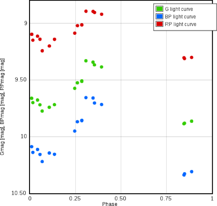
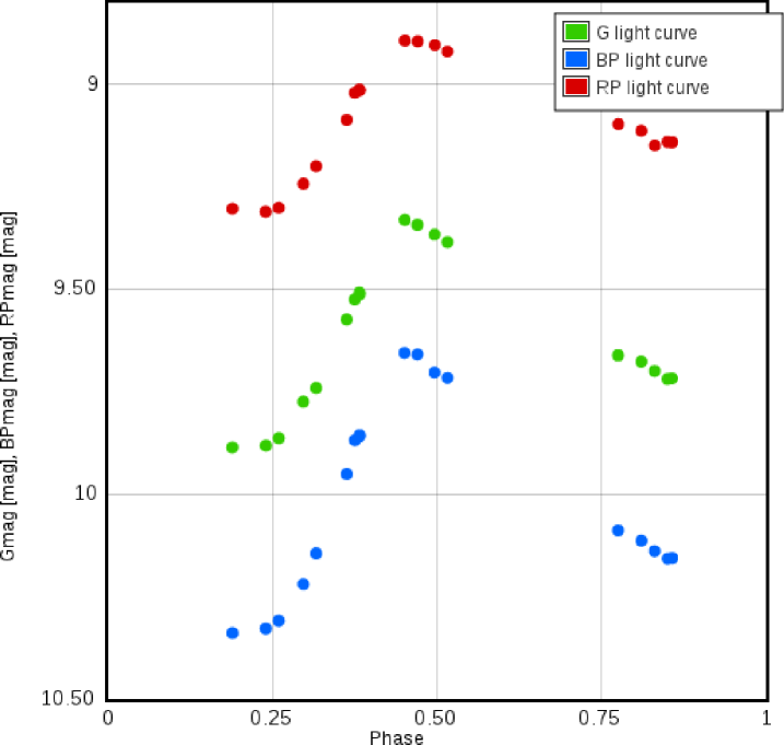
Figure 1: Example of the phased light curve for AD Gem in the Gaia $G$, $Bp$, and $Rp$ bands fitted with the period as given by the SOS (1.895 days, left) and the correct period (3.788 days, right). The plots were made using the tools available through VizieR.

Based on the data in GDR2 some checks were performed against the data that was prepared pre-Gaia. For 279 stars the periods derived by the SOS module compare well to the value in the literature (in Table LABEL:Tab:Targets), with a relative precision better than 0.5% and a median value $\mid\Delta P\mid/P=1.3\cdot 10^{-4}$. Then there is a jump, and for 35 stars the periods are significantly different with $\mid\Delta P\mid/P>0.06$. The most extreme example is V500 Sco with a true period of 9.3 and a derived period of 175.6 days. Other periods differ by a near integer number, for example T Vul (true period of 4.435 and a derived period of 2.217 days) or XX Car (true period of 15.716 and a derived period of 31.449 days). All 35 cases were inspected by folding the Gaia light curve with the period in the literature; the literature period always fits the Gaia light curve better (see Fig. 1 for an example).

In the present sample about 11% of the Cepheids have been assigned an incorrect period. As the paper describing the SOS Cepheid and RR Lyrae module used for GDR2 (Clementini et al., 2018) does not contain any information about the period validation for Cepheids it is unclear how representative this fraction is.

Of interest is also the classification of the objects, and their pulsation mode. Of the 314 stars in the sample analysed by the SOS, 271 classifications agree with the value in the literature. The other 43 cases are listed in Table 3. The most common difference is between the FU and FO pulsations. As noted above some periods are incorrect, and this is indicated as it might have influenced the classification as well.

Table 2: Comparison of pulsation types and modes.

Name	Literature	GDR2	GDR2	Remarks
	(Tab. 1)	SOS	nTran
BG Cru	DCEPS	DCEP-FU	CEP
CI Per	DCEP?	DCEP-FO	T2CEP
CR Cep	DCEP?	DCEP-FU	CEP
CY Aur	DCEP	DCEP-FO	CEP	Period incorrect
DK Vel	DCEP	DCEP-FO	CEP
FM Aql	DCEP	DCEP-FO	CEP	Period incorrect
FO Cas	DCEP	T2CEP	T2CEP
GH Car	DCEPS	DCEP-FU	CEP
IT Car	DCEPS	DCEP-FU	CEP
MY Pup	DCEPS	DCEP-FU	CEP
NT Pup	DCEP	T2CEP	T2CEP
RS Ori	DCEP	DCEP-FO	CEP	Period incorrect
RW Cam	DCEP	T2CEP	CEP
TT Aql	DCEP	DCEP-FO	CEP	Period incorrect
TU Cas	DCEP(B)	DCEP-FU	CEP
TX Del	CWB:	T2CEP	CEP
V1334 Cyg	DCEPS	DCEP-FU	CEP
V350 Sgr	DCEP	DCEP-FO	CEP	Period incorrect
V378 Cen	DCEPS	DCEP-FU	CEP
V482 Sco	DCEP	DCEP-FO	CEP	Period incorrect
V500 Sco	DCEP	T2CEP	CEP	Period incorrect
V636 Cas	DCEPS	DCEP-FU	CEP
V659 Cen	DCEPS	DCEP-FU	CEP
V924 Cyg	DCEPS	DCEP-FU	CEP
X Lac	DCEPS	DCEP-FU	CEP
Y Oph	DCEP?	DCEP-FU	CEP
Y Car	DCEP(B)	DCEP-FO	CEP
GZ Car	DCEP(B)	DCEP-FU	CEP
BK Cen	DCEP(B)	DCEP-FU	CEP
V458 Sct	DCEP(B)	DCEP-FU	CEP	Period incorrect
U TrA	DCEP(B)	DCEP-FU	CEP
V493 Aql	DCEP	MULTI	CEP	Period incorrect
V526 Aql	DCEP	T2CEP	T2CEP	Period incorrect
CO Aur	DCEPS(B)	DCEP-FO	CEP
AC Cam	DCEP	MULTI	-
FW Cas	DCEP	MULTI	-
HK Cas	DCEP	DCEP-FO	ACEP
EK Del	AHB1:	DCEP-FU	ACEP
FQ Lac	CEP:?	DCEP-FU	T2CEP
BE Mon	DCEP	DCEP-FO	CEP
QQ Per	CEP?	T2CEP	T2CEP
CR Ser	DCEP	DCEP-FO	CEP	Period incorrect
V1954 Sgr	DCEP	DCEP-FO	CEP	Period incorrect

Interestingly, the SOS module also provides an iron abundance estimate based on the shape of the $G$-band light curve for 120 objects in the sample. Figure 2 compares the adopted [Fe/H] abundance from the literature listed in Table LABEL:Tab:Targets with the value provided in GDR2. There is a correlation, but with a lot of scatter. A bi-sector fit gives a slope of 0.99 and a zero point of 0.09. The scatter around this relation is 0.26 dex, comparable to the quoted uncertainty of 0.22–0.24 dex (which includes a systematic error of 0.2 dex; see Clementini et al. 2018). This justifies the choice of considering only Cepheids with spectroscopic abundance determinations.

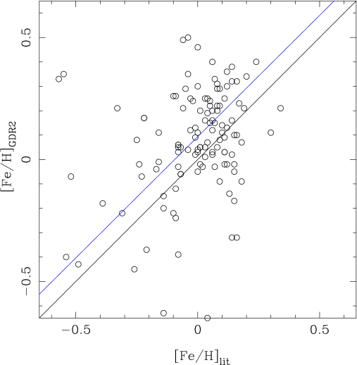
Figure 2: Comparison of the [Fe/H] abundance from the literature to that of the SOS. The black line is the one-to-one relation. The blue line is the bi-sector fit to the data.

Table 4 lists the CCs with accurate external parallaxes (i.e. non-Gaia, non-Hipparcos) and compares them to Gaia DR2, Gaia DR1, and Hipparcos parallaxes. The external parallaxes are mostly based on HST (Benedict et al., 2007; Riess et al., 2014; Casertano et al., 2016; Riess et al., 2018a). Out of interest, the parallax of Polaris B is also listed, with the results from GDR2 and the parallax as recently determined by Bond et al. (2018). Polaris B is thought to be physically related to $\alpha$ UMi (see Anderson 2018 and discussion therein). Another parallax estimate of 10.1 $\pm$ 0.2 mas exists for Polaris A (Turner et al., 2013) based on the claimed membership of a cluster, but this result has been disputed (van Leeuwen, 2013). The photometric parallax of Polaris predicted by the $PL$ relation derived in the present paper is discussed in Appendix B.

What is remarkable in Table 4 is that many of the well-known Cepheids have very poor solutions with very large GOF and excess noise values. There almost seems to be a dichotomy with Cepheids with zero excess noise to have a GOF smaller than 8. Figure 3 shows the relation between these two parameters for the entire sample, and the distribution over the GOF parameter. We note that this distribution is not a Gaussian with mean zero and unit variance, but it is due to the fact that this parameter was not updated after discovery of the DOF bug (Lindegren et al., 2018).

The bottom panel in Figure 3 shows the distribution over the GOF parameter when it is recomputed multiplying the astrometric_chi2_al statistic by a constant for all sources and to force a peak in the histogram near zero. The factor used is 0.7, which is roughly consistent with the information provided in Appendix A in Lindegren et al. (2018).

All nine stars with a GOF smaller than 8 have an accurate external parallax (${\sigma}_{\pi}$ comparable to that in GDR2). The weighted mean difference (in the sense GDR2-external parallax) is $-0.049\pm 0.018$ mas. It is tempting to relate this to the parallax zero-point offset observed for QSO ($-0.029$ mas, Lindegren et al. 2018), based on RGB stars from Kepler and APOGEE data (about $-0.053$ mas, Zinn et al. 2018), eclipsing binaries ($-0.082\pm 0.033$ mas, Stassun & Torres 2018), a sample of 50 CCs ($-0.046\pm 0.013$ mas, Riess et al. 2018b), RR Lyrae stars ($\sim-0.056$ mas, Muraveva et al. 2018), and the value of $-0.0319\pm 0.0008$ mas mentioned for Cepheids in the GDR2 catalogue validation paper (Arenou et al., 2018).

It should be noted that the assumption of a constant parallax zero-point offset is an oversimplification. Lindegren et al. (2018) already show that there are correlations with position on the sky, and trends with magnitude and colour (their Figs. 7, 12, 13).

Binarity is common among Cepheids and has not been discussed so far. Binarity is not considered in solving for the astrometric parameters in GDR2. If binarity has an effect it would express itself in a poor fit when only solving for position, proper motion, and parallax. As noted in Appendix A in Lindegren et al. (2018) the statistical quantities astrometric_chi2_al and the GOF statistic have not been corrected for the DOF bug. The GOF statistic is expected to follow a normal distribution around zero with unit variance, but for the current sample it roughly follows a normal distribution which peaks near 4 and with a clear excess of stars with a GOF $>8$. The models in Appendix A show that selecting on GOF $<8$ removes 40% of the sample. Many of those are known binaries. Riess et al. (2018b) identify three outliers in their sample of 50 CCs, based on the location in a simple ${\sigma}_{\pi}$ versus $\pi$ plot: SV Per, RW Cam, and RY Vel. The GOF statistic of these objects is 84, 85, and 38, respectively, and SV Per and RW Cam show close companions in their HST images. Other known binaries have large GOF statistics and are therefore excluded from the analysis: V1334 Cyg (GOF=37) from Evans (2000) and Gallenne et al. (2013); AX Cir (GOF=387), KN Cen (GOF=8.5), SY Nor (GOF=13), AW Per (GOF=8.6), and SV Per (GOF=85) from Evans (1994), and R Cru (GOF=92) and S Mus (GOF=60) from Evans et al. (2016). It appears that selecting a GOF $<8$ is an effective way of removing binaries from GDR2 data, and suggests that the results are not systematically influenced by binarity in the remaining sample.

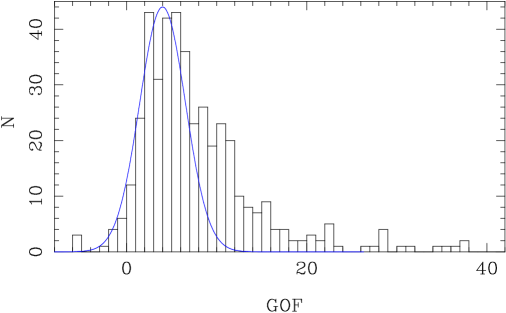
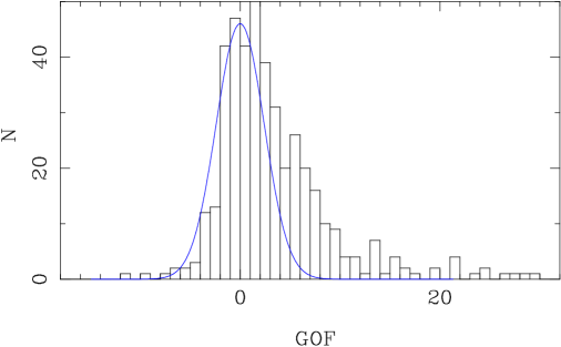
Figure 3: Goodness-of-fit (GOF) parameter plotted against the excess noise, with the inset showing a zoomed-in version. At the extreme end is Polaris with $\epsilon_{i}=7.5$ and GOF= 270 (top panel). For clarity a randomly Gaussian distributed number is added to the excess noise when it is below 0.02 mas in the inset. In the middle panel the histogram of the GOF parameter is shown with a Gaussian distribution (with mean 4.0 and $\sigma=1.8$) overplotted in blue. In the bottom panel the GOF statistic has been recomputed by multiplying the astrometric_chi2_al statistic by 0.7 for all sources to force a peak in the histogram at about zero. The $\sigma$ of the Gaussian is 1.7. The abscissa has been shifted by ten units compared to the plot in the middle panel.

Table 3: Comparison of Gaia data to Hipparcos and HST parallaxes.

Name	$\pi\pm{\sigma}_{\pi}$	GOF	$\epsilon_{i}$	D	$\pi\pm{\sigma}_{\pi}$	$\epsilon_{i}$	R	$\pi\pm{\sigma}_{\pi}$	GOF	R	$\pi\pm{\sigma}_{\pi}$	GOF	R	$\pi\pm{\sigma}_{\pi}$	R	$\pi\pm{\sigma}_{\pi}$	R	$\pi\pm{\sigma}_{\pi}$	R
	(mas)		(mas)		(mas)	(mas)		(mas)			(mas)			(mas)		(mas)		(mas)
$\alpha$ UMi	$\ldots$	271.04	7.46	15200	$\ldots$	$\ldots$	-	7.56 $\pm$ 0.48	1.22	3	7.54 $\pm$ 0.11	1.08	4	7.72 $\pm$ 0.12	5	$\ldots$	-	7.620 $\pm$ 0.080	3,4,5
Polaris B	7.292 $\pm$ 0.028	12.22	0.00	0	$\ldots$	$\ldots$	-	$\ldots$	$\ldots$	-	$\ldots$	$\ldots$	-	$\ldots$	-	6.26 $\pm$ 0.24	10	$\ldots$	-
$\beta$ Dor	3.112 $\pm$ 0.284	170.94	1.62	1340	$\ldots$	$\ldots$	-	3.14 $\pm$ 0.59	$-$0.38	3	3.24 $\pm$ 0.36	13.84	4	3.64 $\pm$ 0.28	5	3.14 $\pm$ 0.16	7	3.256 $\pm$ 0.135	3,5,7
$\delta$ Cep	$-1.172\pm$ 0.468	182.21	2.44	2100	$\ldots$	$\ldots$	-	3.32 $\pm$ 0.58	0.41	3	3.77 $\pm$ 0.16	-2.45	4	3.81 $\pm$ 0.20	5	3.66 $\pm$ 0.15	7	3.723 $\pm$ 0.095	3,4,5,7
FF Aql	1.810 $\pm$ 0.107	65.83	0.49	100	1.64 $\pm$ 0.89	3.14	2	1.32 $\pm$ 0.72	0.43	3	2.11 $\pm$ 0.33	0.77	4	2.05 $\pm$ 0.34	5	2.81 $\pm$ 0.18	7	2.543 $\pm$ 0.143	4,5,7
$l$ Car	0.777 $\pm$ 0.257	171.10	1.67	1190	$\ldots$	$\ldots$	-	2.16 $\pm$ 0.47	$-$0.49	3	2.09 $\pm$ 0.29	5.81	4	2.06 $\pm$ 0.27	5	2.01 $\pm$ 0.20	7	2.042 $\pm$ 0.152	3,5,7
RS Pup	0.584 $\pm$ 0.026	7.74	0.00	0	0.63 $\pm$ 0.26	0.65	2	0.49 $\pm$ 0.68	$-$0.73	3	1.91 $\pm$ 0.65	0.73	4	1.44 $\pm$ 0.51	5	0.524 $\pm$ 0.022	6	$\ldots$	-
RT Aur	1.419 $\pm$ 0.203	52.32	0.77	132	$\ldots$	$\ldots$	-	2.09 $\pm$ 0.89	$-$0.05	3	$-$1.10 $\pm$ 1.41	10.29	4	-0.23 $\pm$ 1.01	5	2.40 $\pm$ 0.19	7	2.40 $\pm$ 0.19	7
SS CMa	0.201 $\pm$ 0.029	4.37	0.00	0	0.69 $\pm$ 0.23	0.35	2	$-$0.37 $\pm$ 1.75	1.32	3	0.40 $\pm$ 1.78	1.81	4	0.35 $\pm$ 1.86	5	0.389 $\pm$ 0.029	9	$\ldots$	-
S Vul	0.305 $\pm$ 0.041	7.98	0.00	0	$-$0.21 $\pm$ 0.43	0.53	2	$\ldots$	$\ldots$	-	$\ldots$	$\ldots$	-	$\ldots$	-	0.322 $\pm$ 0.040	9	$\ldots$	-
SY Aur	0.313 $\pm$ 0.052	3.35	0.00	0	0.69 $\pm$ 0.25	0.48	2	1.15 $\pm$ 1.70	0.27	3	$-$1.84 $\pm$ 1.72	1.31	4	-0.52 $\pm$ 1.44	5	0.428 $\pm$ 0.054	8	$\ldots$	-
T Vul	1.674 $\pm$ 0.089	44.55	0.33	56	$\ldots$	$\ldots$	-	1.95 $\pm$ 0.60	$-$0.24	3	2.71 $\pm$ 0.43	1.37	4	2.31 $\pm$ 0.29	5	1.90 $\pm$ 0.23	7	2.156 $\pm$ 0.166	4,5,7
VX Per	0.330 $\pm$ 0.031	3.81	0.00	0	0.50 $\pm$ 0.27	0.71	2	1.08 $\pm$ 1.48	0.04	3	0.87 $\pm$ 1.52	1.07	4	1.10 $\pm$ 1.62	5	0.420 $\pm$ 0.074	9	$\ldots$	-
VY Car	0.512 $\pm$ 0.041	1.64	0.00	0	0.73 $\pm$ 0.29	0.62	2	1.28 $\pm$ 1.76	2.88	3	0.36 $\pm$ 1.42	4.91	4	1.56 $\pm$ 0.91	5	0.586 $\pm$ 0.044	9	$\ldots$	-
W Sgr	1.180 $\pm$ 0.412	88.20	1.40	371	$\ldots$	$\ldots$	-	1.57 $\pm$ 0.93	0.47	3	3.75 $\pm$ 1.12	10.40	4	2.59 $\pm$ 0.75	5	2.28 $\pm$ 0.20	7	2.28 $\pm$ 0.20	7
WZ Sgr	0.513 $\pm$ 0.077	3.52	0.00	0	$\ldots$	$\ldots$	-	$-$0.75 $\pm$ 1.76	$-$0.40	3	3.50 $\pm$ 1.22	$-$0.12	4	2.46 $\pm$ 1.12	5	0.512 $\pm$ 0.037	9	$\ldots$	-
X Pup	0.302 $\pm$ 0.043	1.20	0.00	0	0.28 $\pm$ 0.29	0.58	2	$-$0.05 $\pm$ 1.10	1.31	3	1.97 $\pm$ 1.26	$-$0.82	4	2.87 $\pm$ 0.92	5	0.277 $\pm$ 0.047	9	$\ldots$	-
X Sgr	3.431 $\pm$ 0.202	73.61	0.78	151	$\ldots$	$\ldots$	-	3.03 $\pm$ 0.94	0.63	3	3.31 $\pm$ 0.26	$-$0.63	4	3.39 $\pm$ 0.21	5	3.00 $\pm$ 0.18	7	3.197 $\pm$ 0.121	4,5,7
XY Car	0.330 $\pm$ 0.027	7.50	0.00	0	0.19 $\pm$ 0.24	0.50	2	$-$0.62 $\pm$ 0.95	$-$0.05	3	$-$1.02 $\pm$ 0.88	0.18	4	$-$0.75 $\pm$ 0.87	5	0.438 $\pm$ 0.047	9	$\ldots$	-
Y Sgr	$-0.470\pm$ 0.280	73.09	0.75	143	$\ldots$	$\ldots$	-	2.52 $\pm$ 0.93	$-$2.19	3	2.64 $\pm$ 0.45	$-$0.92	4	3.73 $\pm$ 0.32	5	2.13 $\pm$ 0.29	7	2.812 $\pm$ 0.194	4,5,7
$\zeta$ Gem	2.250 $\pm$ 0.301	90.10	1.16	389	$\ldots$	$\ldots$	-	2.79 $\pm$ 0.81	$-$0.18	3	2.37 $\pm$ 0.30	1.19	4	2.71 $\pm$ 0.17	5	2.78 $\pm$ 0.18	7	2.689 $\pm$ 0.114	4,5,7

4 Analysis

The fundamental equation between parallax, apparent, and absolute magnitude is

$$\pi=100\cdot 10^{0.2\;(M-m)},$$ (1)

where $\pi$ is the parallax in mas, and $m$ the dereddened apparent magnitude. The absolute magnitude $M$ is parameterised as

$$M=\alpha+\beta\,\log P+\gamma\,{\rm[Fe/H]}$$ (2)

and the aim is to derive the coefficients $\alpha$, $\beta$, and $\gamma$.

Feast & Catchpole (1997) had a similar aim in mind using Hipparcos data. The accuracy of the Hipparcos data was such that only the simpler problem with $\gamma=0$ and known slope $\beta$ (from Cepheids in the Large Magellanic Cloud, LMC) could be tackled. In that case the problem is simplified to $10^{0.2\alpha}=0.01\cdot\pi\cdot 10^{0.2\;(m-\beta\,\log P)}$. The zero point of the $PL$ relation was found by taking the weighted mean of the term on the right-hand side over all 223 Cepheids available to them, and then calculating 5 times the logarithmic value. For an assumed slope of $-2.81$ in the $V$ band they derived $\alpha=-1.43\pm 0.10$ mag. Using the revised Hipparcos parallaxes van Leeuwen et al. (2007) found $\alpha=-2.47\pm 0.03$ mag (the weighted mean of the three values in their Table 6) for fixed $\beta=-3.26$ in the $K$ band, see Table 5.

In the present paper, in principle, we want to solve for all coefficients and therefore the non-linear problem of fitting Eq. 1 is solved directly using the Levenberg–Marquardt algorithm (as implemented in Fortran in Numerical Recipes, Press et al. 1992).

An important advantage of using Eq. 1 in this form is that no selection on positive parallaxes or relative parallax error is required, and therefore the results are not subject to Lutz–Kelker bias (Lutz & Kelker 1973) (see the discussion in Feast & Catchpole 1997; Koen & Laney 1998; Lanoix et al. 1999). It is also one of the methods, known as astrometry-based luminosity (ABL), used in Gaia Collaboration et al. (2017) to analyse GDR1 data (also see Luri et al. 2018) . Another advantage is that the errors in the parallax can be assumed to be symmetric and Gaussian distributed.

Monte Carlo simulations are carried out for an improved understanding of the results. The basic data of the Cepheids (Table LABEL:Tab:Targets) are read in, together with the parameters of the Gaia DR2 (or the external parallax data). Periods of FO pulsators (type DCEPS) are fundamentalised using $P_{0}=P_{1}/(0.716-0.027\,\log P_{1})$ following Feast & Catchpole (1997). Then,

• A new parallax is drawn from a Gaussian with the adopted mean and error. A parallax zero-point offset may be applied;

• A new period is drawn from a Gaussian with the mean input period and an error equal to $1.3\cdot 10^{-4}P$;

• A new [Fe/H] is drawn from a Gaussian with the mean input iron abundance and an error of 0.08 dex;

• A new reddening is drawn from a Gaussian with the mean and error from the input. Negative reddenings are set to zero;

• The input $V,J,H,K$ magnitudes are dereddened (see Sect. 2 for details);

• New $V,J,H,K$ magnitudes are drawn from Gaussians using the dereddened magnitudes and assumed error bars (see Sect. 2 for details);

• The NIR magnitudes are transformed to the 2MASS system if needed;

• To take into account the intrinsic width in the instability strip (see Feast & Catchpole 1997) the value of $(M-m)$ is increased by a value drawn from a Gaussian centred on 0 with error $\delta_{\rm PL}$.

The generated data ($\pi$, ${\sigma}_{\pi}$, magnitude, period, colour, iron abundance) are fed to the minimization routine that returns the parameters ($\alpha$, $\beta$, $\gamma$) with internal error bars. This is repeated $N$ times (typically $N=$1001). The best estimate of the parameters is taken as the median of its distribution with the $1\sigma$ error bar derived from the 2.7% and 93.7% percentiles ($\pm 2\sigma$). This results in realistic error bars that takes into account all likely variations in the data.

Using the best fit parameters ($\alpha,\beta,\gamma$ for each simulation) the photometric parallax is calculated using Eqs. 1 and 2 and compared to the observed parallax. This gives a standard deviation per star and when these values are ordered over all simulations, stars that are systematic outliers can be identified. An rms deviation of the fit to the data is also calculated.

5 Simulations

To test the methodology and the sensitivity to the parameters, simulations were carried out. Parallax and error in the parallax are generated based on the period, reddening, magnitudes of the stars in the sample, and a period-luminosity relation. These observed parameters are then fed to the code and analysed as described above. The results are listed in Table 4. The sample size was chosen to represent the number of FU and FO pulsators in the sample. Solutions 1–4 are idealised: the simulated parallax is exactly 1/distance, and the error in the parallax is based on a fraction of the distance. The input slope and zero point are retrieved almost exactly. In all other simulations the simulated parallax is based on the exact parallax plus a Gaussian distributed error. In solutions 5–8 this is still based on a hypothetical fractional error in the distance. In all other simulations the error in the parallax is based on the observed distribution among the stars with a GOF $<8$. The distribution is not a strong function of $G$-band (or $V$-band) magnitude in the present sample, and ${\sigma}_{\pi}$ is represented by a mean of 0.040 and a Gaussian dispersion of 0.013 with a minimum value of 0.020 mas. Solution 9 is the standard case which returns the input slope and zero point with a slight offset, but still within the error bars. Selecting on parallax error does not influence this (solutions 12 and 13. We note that in the present sample, very few or no negative parallaxes are predicted).

The last part of the simulations investigates the influence of a zero-point offset in the parallax. The all-sky average value derived from QSOs ($-0.029$ mas, Lindegren et al. 2018) and for a sample of 50 CCs ($-0.046$ mas, Riess et al. 2018b) are used to illustrate this.

The impact is significant on both zero point and slope of the $PL$ relation when not considered in the analysis of the data (solutions 14 and 15). The true solution can be partially recovered when the parallax zero-point offset is partially taken into account in the analysis (solutions 16 and 17). Making a strong selection on the relative parallax error or parallax may also recover an unrecognised parallax zero-point offset, but at the expense of a larger error bar in the zero point and slope of the $PL$ relation (solutions 18–21 and 22–24).

The last two entries are for a realistic sample size (see next section), also including an intrinsic width of the instability strip (IS). In both cases this leads to larger error bars in the derived parameters.

Table 4: Simulations of the $PL$ relations of the form $M=\alpha+\beta\log P$ with input values $\alpha=-2.50$ and $\beta=-3.30$; $N$ is the number of stars in the solution.

#	$\alpha$	$\beta$	$N$	Remarks
Using exact distance
1	-2.502 $\pm$ 0.006	-3.296 $\pm$ 0.007	426	1% error on distance
2	-2.502 $\pm$ 0.009	-3.296 $\pm$ 0.011	426	2% error on distance
3	-2.502 $\pm$ 0.018	-3.296 $\pm$ 0.020	426	5% error on distance
4	-2.504 $\pm$ 0.037	-3.294 $\pm$ 0.041	426	10% error on distance
With parallax error
5	-2.499 $\pm$ 0.006	-3.297 $\pm$ 0.007	426	1% error on distance
6	-2.500 $\pm$ 0.009	-3.294 $\pm$ 0.011	426	2% error on distance
7	-2.496 $\pm$ 0.018	-3.293 $\pm$ 0.020	426	5% error on distance
8	-2.488 $\pm$ 0.037	-3.294 $\pm$ 0.041	426	10% error on distance
9	-2.521 $\pm$ 0.021	-3.267 $\pm$ 0.022	426	parallax error based on data
10	-2.518 $\pm$ 0.027	-3.268 $\pm$ 0.030	426	error based on data, another random seed
11	-2.514 $\pm$ 0.023	-3.273 $\pm$ 0.025	426	error based on data, another random seed
12	-2.511 $\pm$ 0.021	-3.276 $\pm$ 0.023	361	error based on data, $\pi>0,{\sigma}_{\pi}/\pi<0.2$
13	-2.514 $\pm$ 0.024	-3.273 $\pm$ 0.027	218	error based on data, $\pi>0,{\sigma}_{\pi}/\pi<0.1$
14	-2.557 $\pm$ 0.022	-3.295 $\pm$ 0.024	426	error based on data, ZPoff= $-0.029$ mas, not in analysis
15	-2.577 $\pm$ 0.022	-3.312 $\pm$ 0.024	426	error based on data, ZPoff= $-0.046$ mas, not in analysis
16	-2.521 $\pm$ 0.022	-3.267 $\pm$ 0.023	426	error based on data, ZPoff= $-0.046$ mas, $-0.046$ in analysis
17	-2.541 $\pm$ 0.022	-3.284 $\pm$ 0.023	426	error based on data, ZPoff= $-0.046$ mas, $-0.029$ in analysis
18	-2.565 $\pm$ 0.023	-3.319 $\pm$ 0.025	310	error based on data, ZPoff= $-0.046$ mas, not in analysis, $\pi>0,{\sigma}_{\pi}/\pi<0.2$
19	-2.562 $\pm$ 0.023	-3.308 $\pm$ 0.024	189	error based on data, ZPoff= $-0.046$ mas, not in analysis, $\pi>0,{\sigma}_{\pi}/\pi<0.1$
20	-2.572 $\pm$ 0.025	-3.271 $\pm$ 0.027	76	error based on data, ZPoff= $-0.046$ mas, not in analysis, $\pi>0,{\sigma}_{\pi}/\pi<0.05$
21	-2.542 $\pm$ 0.040	-3.276 $\pm$ 0.038	13	error based on data, ZPoff= $-0.046$ mas, not in analysis, $\pi>0,{\sigma}_{\pi}/\pi<0.02$
22	-2.575 $\pm$ 0.026	-3.273 $\pm$ 0.028	126	error based on data, ZPoff= $-0.046$ mas, not in analysis, $\pi>0.5$ mas
23	-2.570 $\pm$ 0.030	-3.257 $\pm$ 0.033	50	error based on data, ZPoff= $-0.046$ mas, not in analysis, $\pi>1.0$ mas
24	-2.539 $\pm$ 0.035	-3.279 $\pm$ 0.035	20	error based on data, ZPoff= $-0.046$ mas, not in analysis, $\pi>1.5$ mas
25	-2.515 $\pm$ 0.033	-3.288 $\pm$ 0.039	205	as (9), for realistic sample size and $\delta_{\rm PL}=0$ mag
26	-2.520 $\pm$ 0.058	-3.289 $\pm$ 0.066	205	as (9), for realistic sample size and $\delta_{\rm PL}=0.066$ mag

6 Results

6.1 $PL$ relation

Two sources of parallax data are considered. The first is exclusively based on GDR2 data. However, many bright stars have a very poor astrometric solution and have to be discarded (see Table 4 and the discussion below). In the second sample the poorest GDR2 parallax data (with GOF $>8$) is replaced by external data when available. These are the 11 stars with an entry in the last column of Table 4 (as having a non-Hipparcos based accurate parallax) and 9 stars where the weighted mean of the available Hipparcos parallaxes was used.

For the moment we do not consider the metallicity and concentrate on the classical $PL$ relation in the $V$, $K$, and $WVK$ bands, the Wesenheit reddening-free index defined as $WVK=K-0.13\;(V-K)$ (Ripepi et al., 2012), based on the reddening law of Cardelli et al. (1989). A large number of models was run to investigate the influence of FU versus FO pulsators, period cuts, selection on GOF, the parallax zero-point offset, the intrinsic width of the IS, and to identify systematic outliers. For completeness the model results are reported and briefly discussed in Appendix A. The conclusions are to conservatively use only FU mode pulsators (the FO mode pulsators seem to show a significantly different slope), consider stars between 2.7 and 35 days (mainly for the comparison to SMC and LMC results), and select stars with $\mid$GOF$\mid<8$ and $\epsilon_{i}<0.001$. The stars U Vul, V Vel, V636 Cas, V526 Aql, QQ Per, and HQ Car are also excluded. The last two are likely T2C. The standard values for $\delta_{\rm PL}$ of 0.20, 0.066, and 0.049 mag in the $V$, $K,$ and $WVK$ bands are adopted below (Inno et al., 2016).

Table 5 lists the results for this reduced sample of stars. Solutions 1–9 using only GDR2 parallaxes (marked ‘GDR2’ in the table), solutions 10–12 using external parallaxes when available for the poorest GDR2 data (marked ‘GDR2+Ext’. Any parallax zero-point offset is only applied to the GDR2 objects). In these first solutions zero point and slope of the $PL$ relations are both fitted. For a fixed parallax zero-point offset adding the external parallax data does not have a very big effect (less then 1$\sigma$; solutions 1, 4, 7 versus 10, 11, 12).

The effect of a parallax zero-point offset is larger, and systematic. Increasing the Gaia parallax (making the offset more negative in the convention used by Lindegren et al. 2018) makes the slope less steep and the zero point fainter in all three filters considered.

The slope of the $PL$ relation derived in the $V$, $K$, and $WVK$ filters is different than that in the LMC. Table 6 compiles recent determinations of the $PL(Z)$ relation in these filters in the SMC, LMC, and the Milky Way. They include the zero point and slope derived for Galactic Cepheids using Hipparcos data (Feast & Catchpole, 1997; van Leeuwen et al., 2007), the results by Fouqué et al. (2007) that have been used in the analysis of GDR1 data in Gaia Collaboration et al. (2017). Listed next are the results by Storm et al. (2011a, b) and Groenewegen (2013) from Baade–Wesselink distances to SMC, LMC, and Galactic objects. The solutions for the Galactic and LMC objects are listed, and the solutions for all objects, which then includes a few CCs in the SMC as well. The last sets of entries are based on OGLE data in the $V$ band, sometimes combined with sets of NIR photometry. We note that there is no single slope (and zero point) for the LMC (and SMC) Cepheids. The values depend on the period cut used, but also on more seemingly subtle issues. Inno et al. (2016) discuss the differences with Jacyszyn-Dobrzeniecka et al. (2016) which both use the OGLE-IV catalogue of CCs. In the $I$ band the papers find different slopes ($-3.327\pm 0.001$ versus $-3.313\pm 0.006$) and Inno et al. (2016) trace this back to a difference in the sigma-clipping procedure (removing 3$\sigma$ versus 6$\sigma$ outliers).

In the $V$ band the difference in slope between the LMC ($\sim-2.65$ to $-2.8$) and the GDR2 results ($\sim-2.35$ to $-2.38$) is at the 3–4$\sigma$ level, and larger when applying a parallax zero-point offset. On the other hand, of the three bands considered the $V$ band is the one where the evidence for non-linearity is strongest and where the slope of SMC Cepheids is known to be inconsistent with that of LMC Cepheids (Ngeow et al., 2009, 2015). In the $K$ band the difference in slope between the LMC ($\sim-3.20$ to $-3.35$) and the GDR2 results ($\sim-3.10$ to $-3.15$) is at the 1–2$\sigma$ level, but becomes significant when applying a parallax zero-point offset. In the $WVK$ band the same tendency is seen, the difference in slope between the LMC and the GDR2 results becomes significant when applying a parallax zero-point offset.

In solution 20 and in Table 5 the slope of the $PL$ relation has been fixed to different values found for LMC Cepheids. This has been done for both sources of parallax data, and for different parallax zero-point offsets. For a fixed slope, the difference between the zero points gives the distance modulus (DM) to the LMC, and this is listed in the last column for selected models. The quoted error considers the error in both the Galactic and LMC zero points. The DM depend strongly on the adopted parallax zero-point offset. For an offset of $-0.046$ mas the DM is essentially 18.70 mag based on the $K$ and $WVK$ band (it is 0.1 mag shorter but with a larger error bar in $V$). Adding the external parallax data makes these distances shorter by about 0.02 mag. The current analysis suggests that a DM of $18.493\pm 0.048$ mag (based on the eclipsing binaries; Pietrzyński et al. 2013) or the recommended value of 18.49 $\pm$ 0.09 mag (based on several independent distance indicators; de Grijs et al. 2014) requires a significantly larger offset (in absolute sense) of order $-0.1$ mas. This is comparable to the $-0.118\pm 0.003$ listed in Arenou et al. (2018) for the difference between GDR2 and Hipparcos parallaxes, but larger (in absolute sense) than given by any of the other comparisons listed in their Table 1.

Table 5: $PL$ relations of the form $M=\alpha+\beta\log P$; $N$ is the number of stars in the solution.

	$\alpha$	$\beta$	$N$	Constraints	LMC DM
					(mag)
FU, $2.7<P(d)<35$, $\mid$GOF$\mid<8$, $\epsilon_{i}<0.001$, $\delta_{\rm PL}$ applied.
1	-1.919 $\pm$ 0.119	-2.386 $\pm$ 0.138	194	V, GDR2, ZPoff= $0$ mas
2	-1.875 $\pm$ 0.118	-2.305 $\pm$ 0.136	194	V, GDR2, ZPoff= $-0.029$ mas
3	-1.848 $\pm$ 0.119	-2.260 $\pm$ 0.135	194	V, GDR2, ZPoff= $-0.046$ mas
4	-2.912 $\pm$ 0.058	-3.154 $\pm$ 0.070	194	K, GDR2, ZPoff= $0$ mas
5	-2.866 $\pm$ 0.057	-3.071 $\pm$ 0.068	194	K, GDR2, ZPoff= $-0.029$ mas
6	-2.839 $\pm$ 0.056	-3.028 $\pm$ 0.067	194	K, GDR2, ZPoff= $-0.046$ mas
7	-3.047 $\pm$ 0.055	-3.252 $\pm$ 0.066	194	WVK, GDR2, ZPoff= $0$ mas
8	-2.999 $\pm$ 0.053	-3.170 $\pm$ 0.063	194	WVK, GDR2, ZPoff= $-0.029$ mas
9	-2.972 $\pm$ 0.052	-3.126 $\pm$ 0.063	194	WVK, GDR2, ZPoff= $-0.046$ mas
10	-1.917 $\pm$ 0.118	-2.351 $\pm$ 0.137	205	V, GDR2+Ext, ZPoff= $0$ mas
11	-2.908 $\pm$ 0.057	-3.109 $\pm$ 0.068	205	K, GDR2+Ext, ZPoff= $0$ mas
12	-3.041 $\pm$ 0.053	-3.207 $\pm$ 0.063	205	WVK, GDR2+Ext, ZPoff= $0$ mas
20	-1.728 $\pm$ 0.029	-2.629 fixed	194	V, GDR2, ZPoff= $0$ mas
21	-1.619 $\pm$ 0.029	-2.629 fixed	194	V, GDR2, ZPoff= $-0.029$ mas
22	-1.557 $\pm$ 0.029	-2.629 fixed	194	V, GDR2, ZPoff= $-0.046$ mas
23	-1.690 $\pm$ 0.029	-2.678 fixed	194	V, GDR2, ZPoff= $0$ mas
24	-1.581 $\pm$ 0.030	-2.678 fixed	194	V, GDR2, ZPoff= $-0.029$ mas
25	-1.519 $\pm$ 0.030	-2.678 fixed	194	V, GDR2, ZPoff= $-0.046$ mas
26	-1.589 $\pm$ 0.030	-2.810 fixed	194	V, GDR2, ZPoff= $0$ mas	18.761 $\pm$ 0.030
27	-1.480 $\pm$ 0.030	-2.810 fixed	194	V, GDR2, ZPoff= $-0.029$ mas	18.650
28	-1.418 $\pm$ 0.030	-2.810 fixed	194	V, GDR2, ZPoff= $-0.046$ mas	18.590
29	-1.321 $\pm$ 0.030	-2.810 fixed	194	V, GDR2, ZPoff= $-0.074$ mas	18.493
30	-1.233 $\pm$ 0.030	-2.810 fixed	194	V, GDR2, ZPoff= $-0.100$ mas	18.405
40	-2.879 $\pm$ 0.014	-3.194 fixed	194	K, GDR2, ZPoff= $0$ mas	18.875 $\pm$ 0.017
41	-2.769 $\pm$ 0.014	-3.194 fixed	194	K, GDR2, ZPoff= $-0.029$ mas	18.765
42	-2.707 $\pm$ 0.014	-3.194 fixed	194	K, GDR2, ZPoff= $-0.046$ mas	18.703
43	-2.827 $\pm$ 0.014	-3.260 fixed	194	K, GDR2, ZPoff= $0$ mas	18.880 $\pm$ 0.014
44	-2.717 $\pm$ 0.014	-3.260 fixed	194	K, GDR2, ZPoff= $-0.029$ mas	18.770
45	-2.655 $\pm$ 0.014	-3.260 fixed	194	K, GDR2, ZPoff= $-0.046$ mas	18.708
46	-2.469 $\pm$ 0.013	-3.260 fixed	194	K, GDR2, ZPoff= $-0.100$ mas	18.522
47	-2.800 $\pm$ 0.014	-3.295 fixed	194	K, GDR2, ZPoff= $0$ mas	18.870 $\pm$ 0.022
48	-2.690 $\pm$ 0.014	-3.295 fixed	194	K, GDR2, ZPoff= $-0.029$ mas	18.760
49	-2.628 $\pm$ 0.014	-3.295 fixed	194	K, GDR2, ZPoff= $-0.046$ mas	18.698
50	-2.442 $\pm$ 0.013	-3.295 fixed	194	K, GDR2, ZPoff= $-0.100$ mas	18.512
51	-2.377 $\pm$ 0.013	-3.295 fixed	194	K, GDR2, ZPoff= $-0.120$ mas	18.447
52	-2.745 $\pm$ 0.014	-3.365 fixed	194	K, GDR2, ZPoff= $0$ mas
52	-2.636 $\pm$ 0.014	-3.365 fixed	194	K, GDR2, ZPoff= $-0.029$ mas
53	-2.574 $\pm$ 0.014	-3.365 fixed	194	K, GDR2, ZPoff= $-0.046$ mas
60	-2.997 $\pm$ 0.013	-3.314 fixed	194	WVK, GDR2, ZPoff= $0$ mas
61	-2.887 $\pm$ 0.013	-3.314 fixed	194	WVK, GDR2, ZPoff= $-0.029$ mas
62	-2.825 $\pm$ 0.013	-3.314 fixed	194	WVK, GDR2, ZPoff= $-0.046$ mas
63	-2.793 $\pm$ 0.013	-3.314 fixed	194	WVK, GDR2, ZPoff= $-0.055$ mas
64	-2.988 $\pm$ 0.013	-3.325 fixed	194	WVK, GDR2, ZPoff= $0$ mas	18.858 $\pm$ 0.018
65	-2.878 $\pm$ 0.013	-3.325 fixed	194	WVK, GDR2, ZPoff= $-0.029$ mas	18.748
66	-2.816 $\pm$ 0.013	-3.325 fixed	194	WVK, GDR2, ZPoff= $-0.046$ mas	18.696
67	-2.784 $\pm$ 0.012	-3.325 fixed	194	WVK, GDR2, ZPoff= $-0.055$ mas	18.654
68	-2.714 $\pm$ 0.012	-3.325 fixed	194	WVK, GDR2, ZPoff= $-0.075$ mas	18.584
69	-2.630 $\pm$ 0.012	-3.325 fixed	194	WVK, GDR2, ZPoff= $-0.100$ mas	18.500
70	-1.544 $\pm$ 0.029	-2.629 fixed	205	V, GDR2+Ext, ZPoff= $-0.046$ mas
71	-1.506 $\pm$ 0.030	-2.678 fixed	205	V, GDR2+Ext, ZPoff= $-0.046$ mas
72	-1.404 $\pm$ 0.030	-2.810 fixed	205	V, GDR2+Ext, ZPoff= $-0.046$ mas	18.576 $\pm$ 0.030
73	-2.684 $\pm$ 0.013	-3.194 fixed	205	K, GDR2+Ext, ZPoff= $-0.046$ mas
74	-2.632 $\pm$ 0.013	-3.260 fixed	205	K, GDR2+Ext, ZPoff= $-0.046$ mas	18.685 $\pm$ 0.013
75	-2.604 $\pm$ 0.013	-3.295 fixed	205	K, GDR2+Ext, ZPoff= $-0.046$ mas
76	-2.550 $\pm$ 0.013	-3.365 fixed	205	K, GDR2+Ext, ZPoff= $-0.046$ mas
77	-2.800 $\pm$ 0.012	-3.314 fixed	205	WVK, GDR2+Ext, ZPoff= $-0.046$ mas
78	-2.792 $\pm$ 0.012	-3.325 fixed	205	WVK, GDR2+Ext, ZPoff= $-0.046$ mas	18.662 $\pm$ 0.018

Table 6: $PL(Z)$ relations in the literature of the form $M=\alpha+\beta\log P+\gamma$ [Fe/H] for different galaxies.

Band	Galaxy	N	$\alpha$	$\beta$	$\gamma$	Remarks
Feast & Catchpole (1997)
V	GAL	220	-1.43 $\pm$ 0.10	-2.81 fixed		Hipparcos
van Leeuwen et al. (2007)
K	GAL	220	-2.47 $\pm$ 0.03	-3.26 fixed		Hipparcos
Fouqué et al. (2007)
V	GAL	58	-1.275 $\pm$ 0.023	-2.678 $\pm$ 0.076
K	GAL	58	-2.282 $\pm$ 0.019	-3.365 $\pm$ 0.063
Gaia Collaboration et al. (2017), ABL solutions						GDR1
V	GAL	102	-1.54 $\pm$ 0.10	-2.678 fixed
K	GAL	102	-2.63 $\pm$ 0.10	-3.365 fixed
WVK	GAL	102	-2.87 $\pm$ 0.10	-3.32 fixed
Storm et al. (2011a, b)						Baade–Wesselink distances
V	GAL	70	-1.29 $\pm$ 0.03	-2.67 $\pm$ 0.10
K	GAL	70	-2.33 $\pm$ 0.03	-3.33 $\pm$ 0.09
V	LMC	36	-1.22 $\pm$ 0.03	-2.78 $\pm$ 0.11
K	LMC	36	-2.36 $\pm$ 0.04	-3.28 $\pm$ 0.09
V	ALL	111	-1.24 $\pm$ 0.03	-2.73 $\pm$ 0.07	+0.09 $\pm$ 0.10
K	ALL	111	-2.35 $\pm$ 0.02	-3.30 $\pm$ 0.06	$-0.11$ $\pm$ 0.10
Groenewegen (2013)						Baade–Wesselink distances
V	ALL	160	-1.48 $\pm$ 0.08	-2.40 $\pm$ 0.07
V	GAL	119	-1.68 $\pm$ 0.10	-2.21 $\pm$ 0.09
V	LMC	36	-1.10 $\pm$ 0.17	-2.69 $\pm$ 0.12
V	ALL	160	-1.55 $\pm$ 0.09	-2.33 $\pm$ 0.07	+0.23 $\pm$ 0.11
V	GAL	121	-1.69 $\pm$ 0.10	-2.21 $\pm$ 0.09	+0.17 $\pm$ 0.25
V	LMC	36	-1.09 $\pm$ 0.17	-2.68 $\pm$ 0.12	$-0.14$ $\pm$ 0.35
K	ALL	162	-2.50 $\pm$ 0.08	-3.06 $\pm$ 0.06
K	GAL	121	-2.55 $\pm$ 0.09	-3.03 $\pm$ 0.08
K	LMC	36	-2.26 $\pm$ 0.17	-3.21 $\pm$ 0.13
K	ALL	162	-2.49 $\pm$ 0.08	-3.07 $\pm$ 0.07	$-0.05$ $\pm$ 0.10
K	GAL	121	-2.56 $\pm$ 0.09	-3.03 $\pm$ 0.08	+0.07 $\pm$ 0.20
K	LMC	36	-2.27 $\pm$ 0.18	-3.22 $\pm$ 0.13	+0.19 $\pm$ 0.37
WVK	ALL	158	-2.68 $\pm$ 0.08	-3.12 $\pm$ 0.06
WVK	GAL	120	-2.69 $\pm$ 0.09	-3.12 $\pm$ 0.08
WVK	LMC	36	-2.41 $\pm$ 0.18	-3.27 $\pm$ 0.13
WVK	ALL	158	-2.69 $\pm$ 0.08	-3.11 $\pm$ 0.07	+0.04 $\pm$ 0.10
WVK	GAL	120	-2.72 $\pm$ 0.09	-3.13 $\pm$ 0.08	+0.34 $\pm$ 0.20
WVK	LMC	36	-2.42 $\pm$ 0.18	-3.29 $\pm$ 0.13	+0.23 $\pm$ 0.37
Jacyszyn-Dobrzeniecka et al. (2016)						OGLE-IV, no reddening correction
V	LMC	2365	17.429 $\pm$ 0.004	-2.672 $\pm$ 0.006		all periods
V	LMC	2090	17.399 $\pm$ 0.005	-2.629 $\pm$ 0.007		$\log P>0.4$
V	LMC	280	17.526 $\pm$ 0.010	-2.964 $\pm$ 0.032		$\log P<0.4$
V	SMC	2734	17.984 $\pm$ 0.002	-2.901 $\pm$ 0.005		all periods
V	SMC	978	17.792 $\pm$ 0.006	-2.648 $\pm$ 0.009		$\log P>0.4$
V	SMC	1758	18.001 $\pm$ 0.004	-2.914 $\pm$ 0.015		$\log P<0.4$
Ngeow et al. (2009, 2015)
V	LMC	1675	17.115 $\pm$ 0.015	-2.769 $\pm$ 0.023		all periods
V	LMC	1566	17.143 $\pm$ 0.018	-2.823 $\pm$ 0.031		$\log P<1.0$
V	LMC	109	17.122 $\pm$ 0.195	-2.746 $\pm$ 0.165		$\log P>1.0$
K	LMC	1554	15.996 $\pm$ 0.010	-3.194 $\pm$ 0.015		all periods
V	SMC	912	17.606 $\pm$ 0.028	-2.660 $\pm$ 0.040		all periods
K	SMC	627	16.514 $\pm$ 0.025	-3.213 $\pm$ 0.032		all periods
Ripepi et al. (2012, 2017)
K	LMC	172	16.070 $\pm$ 0.017	-3.295 $\pm$ 0.018
WVK	LMC	172	15.870 $\pm$ 0.013	-3.325 $\pm$ 0.014
K	SMC		16.686 $\pm$ 0.009	-3.513 $\pm$ 0.036		$\log P<0.47$
K	SMC		16.530 $\pm$ 0.018	-3.224 $\pm$ 0.023		$\log P>0.47$
WVK	SMC		16.527 $\pm$ 0.009	-3.567 $\pm$ 0.034		$\log P<0.47$
WVK	SMC		16.375 $\pm$ 0.017	-3.329 $\pm$ 0.021		$\log P>0.47$
Inno et al. (2016)
V	LMC	1526	17.172 $\pm$ 0.001	-2.807 $\pm$ 0.001		all periods
K	LMC	1518	16.053 $\pm$ 0.002	-3.261 $\pm$ 0.003		all periods
WVK	LMC	2170	15.894 $\pm$ 0.002	-3.314 $\pm$ 0.002		all periods

6.2 $PLZ$ relation

In this section the effect of metallicity is considered. Figure 4 shows the histogram over the [Fe/H] abundance of the reduced sample. The abundance ranges from $-0.59$ to $+0.34$ with an average of $+0.03$ and a median of $+0.06$. The mean abundance of CCs in the LMC with individually determined accurate metallicities (22 stars from Luck et al. 1998; Romaniello et al. 2008; Lemasle et al. 2017) is $-0.35\pm 0.05$.

Figure 4: Distribution of the [Fe/H] abundance in the reduced sample of 205 objects.

Table 7 contains the results when fitting the $PLZ$ relation. The content is similar to Table 5; solutions have been derived by either fitting or fixing the slope of the period dependence, for the two sources of parallax data and for various parallax zero-point offsets. For the solutions with fixed slope the DM to the LMC is listed in the last column, using the mean abundance and including the error on the mean abundance for the LMC Cepheids in the error budget.

The parallax zero-point offset again has an important influence on the results. The zero point and slope of the period dependence change only marginally when also fitting for the metallicity dependence, and the metallicity dependence itself is absent to marginal ($\stackrel{{\scriptstyle<}}{{\sim}}$1.5$\sigma$), but there is a degeneracy of the parameters. Adding the external parallax data makes the metallicity effect stronger.

Solutions 120 and higher are calculated for a fixed period dependence to be able to calculate the DM to the LMC. The result is a stronger dependence on metallicity (in an absolute sense) with, depending on the parallax zero-point offset and the filter, a significance that ranges from non-existing to an $\sim 2\sigma$ effect. For a given parallax zero-point offset the LMC DM is found to be smaller by $\sim 0.03-0.08$ mag than when excluding the metallicity term.

Table 7: $PL$ relations of the form $M=\alpha+\beta\log P+\gamma$ [Fe/H]; $N$ is the number of stars in the solution.

	$\alpha$	$\beta$	$\gamma$	$N$	Constraints	LMC DM
						(mag)
FU, $2.7<P(d)<35$, $\mid$GOF$\mid<8$, $\epsilon_{i}<0.001$, $\delta_{\rm PL}$ applied
101	-1.929 $\pm$ 0.120	-2.407 $\pm$ 0.143	0.326 $\pm$ 0.257	194	V, GDR2, ZPoff= $0$ mas
102	-1.879 $\pm$ 0.121	-2.312 $\pm$ 0.142	0.117 $\pm$ 0.254	194	V, GDR2, ZPoff= $-0.029$ mas
103	-1.846 $\pm$ 0.120	-2.259 $\pm$ 0.141	0.001 $\pm$ 0.258	194	V, GDR2, ZPoff= $-0.046$ mas
104	-2.917 $\pm$ 0.060	-3.166 $\pm$ 0.074	0.237 $\pm$ 0.171	194	K, GDR2, ZPoff= $0$ mas
105	-2.865 $\pm$ 0.057	-3.072 $\pm$ 0.072	0.027 $\pm$ 0.164	194	K, GDR2, ZPoff= $-0.029$ mas
106	-2.835 $\pm$ 0.057	-3.020 $\pm$ 0.071	-0.090 $\pm$ 0.159	194	K, GDR2, ZPoff= $-0.046$ mas
107	-3.051 $\pm$ 0.055	-3.266 $\pm$ 0.071	0.223 $\pm$ 0.167	194	WVK, GDR2, ZPoff= $0$ mas
108	-2.999 $\pm$ 0.053	-3.171 $\pm$ 0.067	0.015 $\pm$ 0.161	194	WVK, GDR2, ZPoff= $-0.029$ mas
109	-2.968 $\pm$ 0.052	-3.120 $\pm$ 0.066	-0.102 $\pm$ 0.156	194	WVK, GDR2, ZPoff= $-0.046$ mas
110	-1.916 $\pm$ 0.119	-2.359 $\pm$ 0.136	0.106 $\pm$ 0.239	205	V, GDR2+Ext, ZPoff= $0$ mas
111	-1.834 $\pm$ 0.118	-2.250 $\pm$ 0.136	-0.064 $\pm$ 0.236	205	V, GDR2+Ext, ZPoff= $-0.046$ mas
112	-2.907 $\pm$ 0.058	-3.109 $\pm$ 0.069	-0.003 $\pm$ 0.163	205	K, GDR2+Ext , ZPoff= $0$ mas
113	-2.824 $\pm$ 0.057	-2.999 $\pm$ 0.067	-0.189 $\pm$ 0.139	205	K, GDR2+Ext, ZPoff= $-0.046$ mas
114	-3.041 $\pm$ 0.053	-3.206 $\pm$ 0.065	-0.013 $\pm$ 0.160	205	WVK, GDR2+Ext, ZPoff= $0$ mas
115	-2.976 $\pm$ 0.052	-3.096 $\pm$ 0.062	-0.204 $\pm$ 0.140	205	WVK, GDR2+Ext, ZPoff= $-0.046$ mas
120	-1.617 $\pm$ 0.033	-2.810 fixed	0.388 $\pm$ 0.271	194	V, GDR2, ZPoff= $0$ mas	18.925 $\pm$ 0.102
121	-1.494 $\pm$ 0.033	-2.810 fixed	0.197 $\pm$ 0.278	194	V, GDR2, ZPoff= $-0.029$ mas	18.735 $\pm$ 0.103
122	-1.424 $\pm$ 0.034	-2.810 fixed	0.095 $\pm$ 0.284	194	V, GDR2, ZPoff= $-0.046$ mas	18.629 $\pm$ 0.105
125	-2.846 $\pm$ 0.019	-3.260 fixed	0.252 $\pm$ 0.166	194	K, GDR2, ZPoff= $0$ mas	18.987 $\pm$ 0.062
126	-2.721 $\pm$ 0.017	-3.260 fixed	0.054 $\pm$ 0.162	194	K, GDR2, ZPoff= $-0.029$ mas	18.792 $\pm$ 0.059
127	-2.651 $\pm$ 0.017	-3.260 fixed	-0.053 $\pm$ 0.161	194	K, GDR2, ZPoff= $-0.046$ mas	18.685 $\pm$ 0.059
130	-3.006 $\pm$ 0.018	-3.325 fixed	0.231 $\pm$ 0.166	194	WVK, GDR2, ZPoff= $0$ mas	18.957 $\pm$ 0.063
131	-2.881 $\pm$ 0.016	-3.325 fixed	0.038 $\pm$ 0.156	194	WVK, GDR2, ZPoff= $-0.029$ mas	18.764 $\pm$ 0.058
132	-2.811 $\pm$ 0.016	-3.325 fixed	-0.070 $\pm$ 0.157	194	WVK, GDR2, ZPoff= $-0.046$ mas	18.656 $\pm$ 0.059
140	-1.566 $\pm$ 0.034	-2.810 fixed	0.136 $\pm$ 0.250	205	V, GDR2+Ext, ZPoff= $0$ mas	18.786 $\pm$ 0.094
141	-1.460 $\pm$ 0.034	-2.810 fixed	0.020 $\pm$ 0.254	205	V, GDR2+Ext, ZPoff= $-0.029$ mas	18.639 $\pm$ 0.095
142	-1.400 $\pm$ 0.033	-2.810 fixed	-0.041 $\pm$ 0.260	205	V, GDR2+Ext, ZPoff= $-0.046$ mas	18.558 $\pm$ 0.097
145	-2.789 $\pm$ 0.017	-3.260 fixed	0.013 $\pm$ 0.163	205	K, GDR2+Ext, ZPoff= $0$ mas	18.847 $\pm$ 0.060
146	-2.681$\pm$ 0.016	-3.260 fixed	-0.106 $\pm$ 0.148	205	K, GDR2+Ext, ZPoff= $-0.029$ mas	18.697 $\pm$ 0.055
147	-2.620 $\pm$ 0.016	-3.260 fixed	-0.168 $\pm$ 0.146	205	K, GDR2+Ext, ZPoff= $-0.046$ mas	18.614 $\pm$ 0.054
148	-2.599 $\pm$ 0.016	-3.260 fixed	-0.193 $\pm$ 0.143	205	K, GDR2+Ext, ZPoff= $-0.052$ mas	18.584 $\pm$ 0.053
150	-2.948 $\pm$ 0.017	-3.325 fixed	-0.002 $\pm$ 0.156	205	WVK, GDR2+Ext, ZPoff= $0$ mas	18.817 $\pm$ 0.058
151	-2.840 $\pm$ 0.015	-3.325 fixed	-0.125 $\pm$ 0.146	205	WVK, GDR2+Ext, ZPoff= $-0.029$ mas	18.666 $\pm$ 0.055
152	-2.779 $\pm$ 0.015	-3.325 fixed	-0.188 $\pm$ 0.142	205	WVK, GDR2+Ext, ZPoff= $-0.046$ mas	18.583 $\pm$ 0.058
153	-2.758 $\pm$ 0.015	-3.325 fixed	-0.211 $\pm$ 0.141	205	WVK, GDR2+Ext, ZPoff= $-0.052$ mas	18.554 $\pm$ 0.054
154	-2.713 $\pm$ 0.015	-3.325 fixed	-0.260 $\pm$ 0.140	205	WVK, GDR2+Ext, ZPoff= $-0.065$ mas	18.492 $\pm$ 0.054

Table 8: $PL$ relations of the form $M=\alpha+\beta\log P+\gamma$ [Fe/H] and variation in the parameters; $N$ is the number of stars in the solution.

	$\alpha$	$\beta$	$\gamma$	$N$	Constraints	LMC DM
						(mag)
Standard: FU, $2.7<P(d)<35$, $\mid$GOF$\mid<8$, $\epsilon_{i}<0.001$, $\delta_{\rm PL}$ applied, GDR2+Ext set, ZPoff= $-0.049$ mas
160	$-1.390\pm$ 0.033	$-2.810$ fixed	$-0.051\pm$ 0.260	205	V, standard	18.544 $\pm$ 0.097
161	$-1.470\pm$ 0.060	$-2.810$ fixed	$-0.042\pm$ 0.453	205	V, $\delta_{\rm PL}\cdot 2=0.40$ mag	18.627 $\pm$ 0.170
162	$-1.372\pm$ 0.035	$-2.810$ fixed	$-0.149\pm$ 0.280	205	V, ${\sigma}_{\pi}\cdot 1.5$ for GDR2	18.492 $\pm$ 0.104
163	$-1.442\pm$ 0.032	$-2.810$ fixed	$-0.084\pm$ 0.248	205	V, $E(B-V)\cdot 1.05$	18.585 $\pm$ 0.093
164	$-1.394\pm$ 0.039	$-2.810$ fixed	$-0.005\pm$ 0.264	205	V, other pick of Iron abundance	18.564 $\pm$ 0.100
165	$-1.388\pm$ 0.033	$-2.810$ fixed	$-0.060\pm$ 0.268	205	V, $\sigma_{\rm[Fe/H]}=0.04$ dex	18.539 $\pm$ 0.099
166	$-1.405\pm$ 0.053	$-2.810$ fixed	$-0.230\pm$ 0.443	28	V, ${\sigma}_{\pi}/\pi<0.05$	18.497 $\pm$ 0.164
167	$-1.389\pm$ 0.033	$-2.810$ fixed	$+0.010\pm$ 0.262	208	V, $P>2.7$d	18.565 $\pm$ 0.097
168	$-1.385\pm$ 0.033	$-2.810$ fixed	$-0.047\pm$ 0.243	217	V, $P>2.0$d	18.541 $\pm$ 0.091
170	$-2.610\pm$ 0.016	$-3.260$ fixed	$-0.182\pm$ 0.145	205	K, standard	18.599 $\pm$ 0.054
171	$-2.618\pm$ 0.023	$-3.260$ fixed	$-0.183\pm$ 0.177	205	K, $\delta_{\rm PL}\cdot 2=0.13$ mag	18.607 $\pm$ 0.067
172	$-2.584\pm$ 0.019	$-3.260$ fixed	$-0.279\pm$ 0.164	205	K, ${\sigma}_{\pi}\cdot 1.5$ for GDR2	18.539 $\pm$ 0.062
173	$-2.614\pm$ 0.016	$-3.260$ fixed	$-0.185\pm$ 0.146	205	K, $E(B-V)\cdot 1.05$	18.602 $\pm$ 0.054
174	$-2.591\pm$ 0.016	$-3.260$ fixed	$-0.171\pm$ 0.143	205	K, $A_{K}/A_{V}=0.10$	18.584 $\pm$ 0.053
175	$-2.611\pm$ 0.019	$-3.260$ fixed	$-0.113\pm$ 0.157	205	K, other pick of Iron abundance	18.624 $\pm$ 0.058
176	$-2.604\pm$ 0.016	$-3.260$ fixed	$-0.259\pm$ 0.140	205	K, $\sigma_{\rm[Fe/H]}=0.04$ dex	18.566 $\pm$ 0.053
177	$-2.602\pm$ 0.025	$-3.260$ fixed	$-0.267\pm$ 0.260	28	K, ${\sigma}_{\pi}/\pi<0.05$	18.562 $\pm$ 0.095
178	$-2.609\pm$ 0.017	$-3.260$ fixed	$-0.141\pm$ 0.151	208	K, $P>2.7$d	18.612 $\pm$ 0.056
179	$-2.605\pm$ 0.016	$-3.260$ fixed	$-0.207\pm$ 0.146	217	K, $P>2.0$d	18.586 $\pm$ 0.055
180	$-2.769\pm$ 0.015	$-3.325$ fixed	$-0.200\pm$ 0.141	205	WVK, standard	18.569 $\pm$ 0.054
181	$-2.773\pm$ 0.019	$-3.325$ fixed	$-0.197\pm$ 0.157	205	WVK, $\delta_{\rm PL}\cdot 2=0.09$ mag	18.574 $\pm$ 0.060
182	$-2.741\pm$ 0.018	$-3.325$ fixed	$-0.297\pm$ 0.166	205	WVK, ${\sigma}_{\pi}\cdot 1.5$ for GDR2	18.507 $\pm$ 0.064
183	$-2.769\pm$ 0.015	$-3.325$ fixed	$-0.200\pm$ 0.141	205	WVK, $E(B-V)\cdot 1.05$	18.569 $\pm$ 0.054
184	$-2.748\pm$ 0.015	$-3.325$ fixed	$-0.186\pm$ 0.141	205	WVK, $A_{K}/A_{V}=0.10$	18.553 $\pm$ 0.054
185	$-2.770\pm$ 0.019	$-3.325$ fixed	$-0.126\pm$ 0.155	205	WVK, other pick of Iron abundance	18.596 $\pm$ 0.059
186	$-2.762\pm$ 0.015	$-3.325$ fixed	$-0.285\pm$ 0.133	205	WVK, $\sigma_{\rm[Fe/H]}=0.04$ dex	18.532 $\pm$ 0.053
187	$-2.768\pm$ 0.015	$-3.325$ fixed	$-0.199\pm$ 0.143	205	WVK, $\sigma_{V}\cdot 2$, $\sigma_{K}\cdot 2$	18.568 $\pm$ 0.055
188	$-2.784\pm$ 0.015	$-3.325$ fixed	$-0.191\pm$ 0.145	205	WVK, No NIR transformation	18.587 $\pm$ 0.055
189	$-2.756\pm$ 0.024	$-3.325$ fixed	$-0.273\pm$ 0.247	28	WVK, ${\sigma}_{\pi}/\pi<0.05$	18.530 $\pm$ 0.092
190	$-2.768\pm$ 0.016	$-3.325$ fixed	$-0.158\pm$ 0.147	208	WVK, $P>2.7$d	18.583 $\pm$ 0.056
191	$-2.763\pm$ 0.015	$-3.325$ fixed	$-0.224\pm$ 0.140	217	WVK, $P>2.0$d	18.555 $\pm$ 0.054
200	$-1.840\pm$ 0.118	$-2.243\pm$ 0.137	0.0 fixed	205	V, standard
201	$-2.827\pm$ 0.055	$-3.000\pm$ 0.065	0.0 fixed	205	K, standard
202	$-2.961\pm$ 0.051	$-3.098\pm$ 0.060	0.0 fixed	205	WVK, standard

7 Discussion and summary

From an initial sample of 452 Galactic Cepheids with accurate [Fe/H] abundances, period-luminosity and period-luminosity-metallicity relations have been derived based on parallax data from Gaia DR2, supplemented with accurate non-Gaia parallax data when available, for a final sample of about 200 FU mode Cepheids with good astrometric solutions.

The influence of a parallax zero-point offset on the derived $PL(Z)$ relation is large, which means that the current GDR2 results do not allow us to improve on the existing calibration of the relation or on the distance to the LMC. The zero point, the slope of the period dependence, and any metallicity dependence of the $PL(Z)$ relations are correlated with any assumed parallax zero-point offset.

Based on a comparison for nine CCs with the best non-Gaia parallaxes (mostly from HST data) a parallax zero-point offset of $-0.049\pm 0.018$ mas, consistent with other values that appeared in the literature after the release of GDR2, is derived from RGB stars using Kepler and APOGEE data (about $-0.053$ mas, Zinn et al. 2018), eclipsing binaries ($-0.082\pm 0.033$ mas, Stassun & Torres 2018), a sample of 50 CCs ($-0.046\pm 0.013$ mas, Riess et al. 2018b), and RR Lyrae stars ($\sim-0.056$ mas, Muraveva et al. 2018).

For a parallax zero-point offset of $-0.049$ mas a final list of calculations, investigating the influence of some other parameters is given Table 8. The slope of the period dependence has been fixed (solutions 160–190), and the resulting DM to the LMC is listed in the last column. Variations in the assumed dispersion in the photometry, reddening, or period cuts have a relatively small impact on the results (especially in $K$ and $WVK$). These models address some concerns that might arise when combining many sources of photometry, reddening, and iron abundances from the literature. Increasing the error in the mean $V$ and $K$ magnitude, or not applying a transformation of the different NIR magnitude systems at all has very little impact.

The most noticeable effect is when the parallax errors in GDR2 are underestimated as this changes the weight of the GDR2 sample with respect to the stars with a non-Gaia parallax. Lindegren et al. (2018) in their Appendix A hint at the fact that the errors in the five astrometric parameters may still be underestimated even after correcting for the DOF bug. This issue will likely be resolved in future releases. The next most important effect is the iron abundance. A smaller error in its determination would help, but equally important is a homogeneous metallicity scale (see Proxauf et al. 2018 for new efforts in this direction).

Solutions 200–202 give the current best estimate of the $PL$ relation (for the assumed parallax zero-point offset), without a metallicity dependence as the current data and analysis does not allow us to prove or disprove a dependence. Figure 5 shows these relations in the three bands considered. No additional sigma-clipping in magnitude space has been applied (as is common in deriving $PL$ relations in the LMC). Only stars that were systematic outliers in $\sigma$-space have been removed, as explained in Sect. 6. As noted before, the slopes of the galactic $PL$ relation are shallower than those derived in the LMC by $\sim 3\sigma$ (for the assumed parallax zero-point offset). If the slope is fixed to values that have been derived for LMC Cepheids, the derived parallax zero-point offset suggests a LMC DM that is larger than commonly adopted. Conversely, a LMC DM of around 18.50 requires a zero-point offset closer to $-0.1$ mas.

The results in this paper show that the parallax zero-point offset should be known to a level of $\raisebox{-3.1298pt}{$\stackrel{{\scriptstyle<}}{{\sim}}$}3\leavevmode\nobreak\ \mu$as to have a $\stackrel{{\scriptstyle<}}{{\sim}}$0.01 mag effect on zero point of the $PL$ relation and the DM to the LMC. It will remain important to have accurate non-Gaia based parallaxes as a control sample, like the ongoing programme using HST (Riess et al., 2014; Casertano et al., 2016; Riess et al., 2018a).

Figure 5: $PL$ relations in the $V$, $K$, and $WVK$ bands (solutions 200–202 from Table 8). For each filter the second panel gives the deviation between observed and predicted parallax (limited to $\pm 5\leavevmode\nobreak\ \sigma$).

Appendix A Initial run of models

Table LABEL:Tab:App1 shows the results of fitting period-luminosity relations in the $V$, $K$, and $WVK$ bands based on several selection criteria, which include the goodness of fit, fundamental or overtone pulsators, period cuts, and parallax zero-point offsets. This initial set of models was calculated to investigate the parameter space and arrive at a ‘best’ sample, which is used in the main text.

The table is organised as follows. The models are grouped by the parallax that was used, GDR2-only or GDR2+External values, as outlined in Sect. 6, and by filter ($V$, $K$, or $WVK$). Then the solutions are given applying the various constraints listed in Col. 4.

Inspecting the results shows that the overtone pulsators (using their fundamentalised period) have significantly different $PL$ relations than the FU mode pulsators. This was not investigated further, but led to the conservative choice of using only FU mode Cepheids in the final sample.

A cut on period was investigated and finally implemented (period between 2.7 and 35 days). The exact values are less important, but they were used to avoid a possible contamination by unrecognised overtone pulsators (at the short period end) and to make a fairer comparison to samples in the Magellanic Clouds where such period cuts are typically used.

Stars for the final sample were selected to have $\mid$GOF$\mid<8$ and no excess noise. This is related to the problem of very poor astrometric solutions, which can occur for the brightest stars, but also due to binarity (see main text).

Appendix B The Polaris system

In this appendix we discuss the distance to the Polaris system, the CC $\alpha$ UMi (Polaris A) and its companion Polaris B, located at about 18″. Polaris A is listed in GDR2 with the largest GOF of the CCs in the sample and without parallax. The parallax used is the average of the available Hipparcos parallaxes (Table 4), but as FO pulsators are excluded in the final analysis, Polaris A is not actually used in this paper. Polaris B is listed in GDR2 with a parallax of 7.292 $\pm$ 0.028 mas. The astrometric solution has zero excess noise and a GOF value of about 12, which means it would not make it through the selection criterion of GOF $<8$ that was applied to the CCs in the sample.

Polaris B has a recent HST based parallax of 6.26 $\pm$ 0.26 mas (Bond et al., 2018) which differs by 4$\sigma$ from the GDR2 value. Anderson (2018) showed that adopting the parallax by Bond et al. (2018) for Polaris A a consistent picture emerged of Polaris as a 7 M_⊙ first-overtone CC near the hot boundary of the first IS crossing. This conclusion was based on the Geneva set of rotating stellar evolutionary models (Anderson et al., 2016) and considering various constraints (the rate of period change, the Wesenheit $WVI$ $PL$ relation, the location in the $M_{V}-(B-V)$ colour-magnitude diagram, the interferometrically determined radius, spectroscopic N/C and N/O abundance ratios, and a dynamical mass measurement). Anderson (2018) does not discuss the quality of the model that can be obtained using the larger Hipparcos parallax.

Based on the current best estimates of the $PL$ relations (solutions 200–202 in Table 8) the photometric parallax of Polaris A is predicted using Monte Carlo simulations, that is, taking into account the uncertainty in $V$ and $K$ photometry and reddening value, and the width of the instability strip. A fundamentalised period of 5.673 days is used. The results are listed in Table 9.

For the standard case the predicted parallax distribution based on the $WVK$ relation gives a median and dispersion (based on 1.483 $\times$ the median absolute deviation, which is equivalent to $\sigma$ in the case of a Gaussian distribution) of 6.99 $\pm$ 0.19 mas. The $K$ band gives a consistent result of 7.12 $\pm$ 0.23 mas; the $V$ band also gives a consistent, but more uncertain, value of 8.1 $\pm$ 0.8 mas. Figure 6 shows the distribution in predicted parallax based on the $WVK$ $PL$ relation and compares it to the various estimates in the literature. These parallax estimates depend on the assumed parallax zero-point offset, and Table 9 list values for some other offsets for the Wesenheit $WVK$ magnitude only, as it gives the best precision.

The calculations and the resulting parallax distribution have assumed so far that Polaris A is located in the centre of the IS with the width of the IS represented by a Gaussian with width $\delta_{\rm PL}=0.049$ mag. Anderson (2018) have argued that Polaris A is located at the blue edge (i.e. the hotter end) of the IS (based on the shorter parallax by Bond et al. 2018). Adding +0.1 mag to the $WVK$ colour of Polaris A to simulate the colour it would have at the centre of the IS results in a parallax estimate of 6.69 $\pm$ 0.10 mas (assuming $\delta_{\rm PL}=0$ mag now).

A particular problem for Polaris A is that its $K$-band magnitude is not very well established, and that interferometric observations have revealed a small excess of 0.016 $\pm$ 0.004 mag in $K$ (Mérand et al., 2006) due to the presence of an extended circumstellar envelope. Making the standard adopted value (see the main text) of $K=0.652\pm 0.028$ mag fainter by this amount (and adding the error in quadrature) has a small effect. The actual value has a potentially larger impact. van Leeuwen et al. (2007) also use the COBE-DIRBE flux of Polaris, but adopting a different calibration scheme and magnitudes for Procyon arrive at $J$ = 0.98 mag and $K$ = 0.60 mag on the SAAO system (with no error bars given). Using the transformation formulae in Carpenter (2001), we arrive at $K=0.58$ mag on the 2MASS system. Using this value (with the same error bar of 0.028 mag as we derived) results in a significantly larger parallax.

In summary, the predicted photometric parallax is not conclusive. It is roughly halfway between the Hipparcos parallax estimates for Polaris A and the GDR2 estimate for Polaris B, and the estimate by Bond et al. (2018).

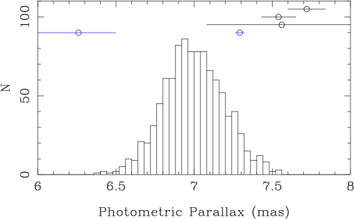
Figure 6: Distribution of the photometric parallax predicted for Polaris based on the $WVK$ $PL$ relation. The blue lines give the parallax and error determined for Polaris B (6.3 mas from Bond et al. 2018, 7.3 mas from GDR2) and the black lines the various estimates from Hipparcos for Polaris A (see Table 4).

Table 9: Photometric parallax predictions for Polaris.

parallax	Remarks
(mas)
6.989 $\pm$ 0.186	WVK (Sol. 200 from Tab. 8)
7.122 $\pm$ 0.234	K (Sol. 201)
8.080 $\pm$ 0.759	V (Sol. 202)
6.484 $\pm$ 0.174	WVK, ZPoff= $0.0$ mas
6.782 $\pm$ 0.181	WVK, ZPoff= $-0.029$ mas
6.989 $\pm$ 0.186	WVK, ZPoff= $-0.049$ mas (Sol. 200)
7.103 $\pm$ 0.189	WVK, ZPoff= $-0.060$ mas
7.310 $\pm$ 0.194	WVK, ZPoff= $-0.080$ mas
7.515 $\pm$ 0.198	WVK, ZPoff= $-0.100$ mas
6.687 $\pm$ 0.102	WVK, ZPoff= $-0.049$ mas, location in the IS, $WVK+0.1$ mag, $\delta_{\rm PL}=0$ mag
6.931 $\pm$ 0.185	WVK, ZPoff= $-0.049$ mas, NIR excess, $\Delta K$= 0.016 $\pm$ 0.004 mag
7.256 $\pm$ 0.194	WVK, ZPoff= $-0.049$ mas, alternative $K$ mag, $K=0.58\pm 0.028$ mag

1]

Table 1: Sample of stars. [TABEL IS AVAILABLE AT THE CDS]

Name	Type	Period	$V$	Ref	$J$	$H$	$K$	Ref	$E(B-V)$	Ref	[Fe/H]1	[Fe/H]2	[Fe/H]3
		(d)	(mag)		(mag)	(mag)	(mag)		(mag)
AA Gem	DCEP	11.302	9.720	1	7.646	7.189	7.086	(1)	0.345 $\pm$ 0.036	(1)	-0.08 2	-0.14 3	-0.22 5
AA Mon	DCEP	3.938	12.740	1	9.729	9.186	8.989	(1)	0.765 $\pm$ 0.017	(1)	-0.12 1	-0.09 3	-0.15 5
AB Cam	DCEP	5.788	11.860	1	9.418	8.936	8.746	(7)	0.622 $\pm$ 0.035	(1)	-0.11 1	-0.07 4	-0.03 5
AC Mon	DCEP	8.014	10.100	1	7.579	7.054	6.885	(1)	0.507 $\pm$ 0.033	(1)	-0.06 1	-0.03 3	-0.17 5
AD Cam	DCEP	11.261	12.560	1	8.988	8.363	8.109	(7)	0.873 $\pm$ 0.012	(1)	-0.28 1	-0.25 4	-0.17 5
AD Cru	DCEP	6.398	11.060	1	8.198	7.661	7.387	(7)	0.640 $\pm$ 0.012	(1)	0.08 1	0.11 3	0.11 5
AD Gem	DCEP	3.788	9.850	1	8.468	8.140	8.066	(1)	0.206 $\pm$ 0.048	(1)	-0.14 1	-0.15 3	-0.11 5
AD Pup	DCEP	13.596	9.920	1	7.723	7.341	7.144	(7)	0.363 $\pm$ 0.020	(1)	-0.06 1	-0.03 3	-0.12 5
AE Tau	DCEP	3.897	11.700	1	9.442	8.949	8.750	(7)	0.568 $\pm$ 0.056	(1)	-0.21 1	-0.18 3	-0.14 5
AE Vel	DCEP	7.134	10.240	1	7.589	7.096	6.867	(7)	0.691 $\pm$ 0.055	(1)	0.11 1	0.14 3	0.11 5
AG Cru	DCEP	3.837	8.220	1	6.629	6.368	6.200	(6)(10) = 5	0.242 $\pm$ 0.020	(1)	0.05 1	0.08 3	-0.08 5
AH Vel	DCEPS	4.227	5.690	1	4.568	4.327	4.235	(3)	0.036 $\pm$ 0.019	(1)	0.09 1	0.19 3	0.11 5
alf UMi	DCEPS	3.970	1.980	1	0.941	0.460	0.652	(13)	0.016 $\pm$ 0.009	(1)			0.15 5
AN Aur	DCEP	10.291	10.450	1	7.932	7.434	7.274	(1)	0.542 $\pm$ 0.040	(1)	-0.13 1	-0.10 3	-0.10 5
AO Aur	DCEP	6.763	10.850	1	8.640	8.188	8.064	(1)	0.437 $\pm$ 0.044	(1)	-0.27 1	-0.26 4	-0.21 5
AO CMa	DCEP	5.816	12.070	1	9.154	8.595	8.366	(3)	0.694 $\pm$ 0.069	(1)	0.01 1		-0.09 5
AP Pup	DCEP	5.084	7.380	1	5.788	5.443	5.322	(3)	0.250 $\pm$ 0.034	(1)	-0.02 1	0.08 3	0.06 5
AP Sgr	DCEP	5.058	6.950	1	5.350	4.970	4.890	(6)	0.184 $\pm$ 0.015	(1)	0.16 1	0.17 3	0.15 5
AQ Car	DCEP	9.769	8.850	1	7.164	6.811	6.573	(10)(11) = 2	0.168 $\pm$ 0.013	(1)	-0.16 1	0.03 3	0.06 5
AQ Pup	DCEP	30.149	8.710	1	6.099	5.481	5.297	(2)	0.531 $\pm$ 0.017	(1)	0.06 1	0.04 3	-0.03 5
AS Per	DCEP	4.973	9.720	1	6.934	6.465	6.295	(1)	0.684 $\pm$ 0.041	(1)	0.11 1	0.14 3	0.15 5
AT Pup	DCEP	6.665	7.980	1	6.289	5.963	5.866	(10)	0.166 $\pm$ 0.011	(1)	-0.08 1	0.05 3	-0.09 5
AV Cir	DCEPS	3.065	7.410	1	5.582	5.236	5.093	(3)	0.374 $\pm$ 0.011	(1)	0.14 1	0.17 3	0.15 5
AV Sgr	DCEP	15.415	11.290	1	6.878	6.089	5.730	(3)	1.238 $\pm$ 0.027	(1)	0.35 1	0.41 3	0.40 5

Table 1: continued.

1]

Table A.1: $PL$ relations of the form $M=\alpha+\beta\log P$; $N$ is the number of stars in the solution.

$\alpha$	$\beta$	$N$	Constraints
GDR2 parallaxes
$V$ band
-1.984 $\pm$ 0.121	-2.326 $\pm$ 0.115	425	all
-1.985 $\pm$ 0.136	-2.321 $\pm$ 0.134	419	$\mid$GOF$\mid<100$
-1.956 $\pm$ 0.043	-2.337 $\pm$ 0.049	376	$\mid$GOF$\mid<20$
-2.033 $\pm$ 0.051	-2.220 $\pm$ 0.061	293	$\mid$GOF$\mid<10$
-2.049 $\pm$ 0.055	-2.201 $\pm$ 0.066	250	$\mid$GOF$\mid<8$
-2.138 $\pm$ 0.074	-2.084 $\pm$ 0.092	197	$\mid$GOF$\mid<6$
-2.134 $\pm$ 0.090	-2.093 $\pm$ 0.110	113	$\mid$GOF$\mid<4$
-2.047 $\pm$ 0.055	-2.202 $\pm$ 0.067	248	$\mid$GOF$\mid<8$, $\epsilon_{i}<0.001$
			$\mid$GOF$\mid<8$, $\epsilon_{i}<0.001$, and …
-1.881 $\pm$ 0.057	-2.416 $\pm$ 0.065	211	FU
-2.661 $\pm$ 0.176	-1.344 $\pm$ 0.247	37	FO
-1.852 $\pm$ 0.060	-2.446 $\pm$ 0.068	205	FU, $P>$2.5d
-1.857 $\pm$ 0.060	-2.441 $\pm$ 0.068	200	FU, $P>$3.0d
-1.869 $\pm$ 0.059	-2.431 $\pm$ 0.070	185	FU, $P>$3.5d
-1.911 $\pm$ 0.080	-2.393 $\pm$ 0.093	159	FU, $P>$2.5d, $\mid$GOF$\mid<6$
-1.882 $\pm$ 0.115	-2.363 $\pm$ 0.131	90	FU, $P>$2.5d, $\mid$GOF$\mid<4$
-1.847 $\pm$ 0.072	-2.457 $\pm$ 0.086	202	FU, $P>$2.5d, $P<$35
-1.886 $\pm$ 0.060	-2.415 $\pm$ 0.068	207	FU, no uncertain types
-1.794 $\pm$ 0.058	-2.385 $\pm$ 0.066	205	FU, $P>$2.5d, ZPoff= $-0.029$ mas
-1.759 $\pm$ 0.057	-2.353 $\pm$ 0.065	205	FU, $P>$2.5d, ZPoff= $-0.046$ mas
-1.883 $\pm$ 0.113	-2.443 $\pm$ 0.126	205	FU, $P>$2.5d, $\delta_{\rm PL}=0.20$
$K$ band
-2.980 $\pm$ 0.031	-3.060 $\pm$ 0.038	425	all
-2.985 $\pm$ 0.029	-3.051 $\pm$ 0.035	419	$\mid$GOF$\mid<100$
-3.008 $\pm$ 0.031	-3.023 $\pm$ 0.036	376	$\mid$GOF$\mid<20$
-3.073 $\pm$ 0.036	-2.929 $\pm$ 0.045	294	$\mid$GOF$\mid<10$
-3.083 $\pm$ 0.039	-2.907 $\pm$ 0.048	250	$\mid$GOF$\mid<8$
-3.171 $\pm$ 0.053	-2.787 $\pm$ 0.067	197	$\mid$GOF$\mid<6$
-3.209 $\pm$ 0.063	-2.769 $\pm$ 0.081	113	$\mid$GOF$\mid<4$
-3.081 $\pm$ 0.039	-2.907 $\pm$ 0.045	248	$\mid$GOF$\mid<8$, $\epsilon_{i}<0.001$
			$\mid$GOF$\mid<8$, $\epsilon_{i}<0.001$, and …
-2.985 $\pm$ 0.041	-3.083 $\pm$ 0.048	211	FU
-3.622 $\pm$ 0.125	-1.974 $\pm$ 0.192	37	FO
-2.953 $\pm$ 0.044	-3.119 $\pm$ 0.051	205	FU, $P>$2.5d
-2.964 $\pm$ 0.044	-3.107 $\pm$ 0.052	200	FU, $P>$3.0d
-2.992 $\pm$ 0.052	-3.079 $\pm$ 0.060	185	FU, $P>$3.5d
-3.017 $\pm$ 0.057	-3.053 $\pm$ 0.069	159	FU, $P>$2.5d, $\mid$GOF$\mid<6$
-3.146 $\pm$ 0.075	-2.869 $\pm$ 0.094	90	FU, $P>$2.5d, $\mid$GOF$\mid<4$
-3.181 $\pm$ 0.091	-2.829 $\pm$ 0.107	76	FU, $P>$3.5d, $\mid$GOF$\mid<4$
-2.957 $\pm$ 0.044	-3.117 $\pm$ 0.053	201	FU, $P>$2.5d, no uncertain
-2.918 $\pm$ 0.047	-3.166 $\pm$ 0.060	202	FU, $P>$2.5d, $P<$35
-2.894 $\pm$ 0.042	-3.055 $\pm$ 0.048	205	FU, $P>$2.5d, ZPoff= $-0.029$ mas
-2.861 $\pm$ 0.040	-3.021 $\pm$ 0.047	205	FU, $P>$2.5d, ZPoff= $-0.046$ mas
-2.957 $\pm$ 0.053	-3.114 $\pm$ 0.061	205	FU, $P>$2.5d, $\delta_{\rm PL}=0.066$
$WVK$ band
-3.114 $\pm$ 0.031	-3.158 $\pm$ 0.038	425	all
-3.118 $\pm$ 0.030	-3.149 $\pm$ 0.036	419	$\mid$GOF$\mid<100$
-3.149 $\pm$ 0.031	-3.113 $\pm$ 0.037	376	$\mid$GOF$\mid<20$
-3.213 $\pm$ 0.035	-3.020 $\pm$ 0.045	293	$\mid$GOF$\mid<10$
-3.221 $\pm$ 0.038	-2.998 $\pm$ 0.048	250	$\mid$GOF$\mid<8$
-3.311 $\pm$ 0.052	-2.876 $\pm$ 0.068	197	$\mid$GOF$\mid<6$
-3.360 $\pm$ 0.063	-2.849 $\pm$ 0.082	113	$\mid$GOF$\mid<4$
-3.221 $\pm$ 0.038	-2.998 $\pm$ 0.045	248	$\mid$GOF$\mid<8$, $\epsilon_{i}<0.001$
			$\mid$GOF$\mid<8$, $\epsilon_{i}<0.001$, and …
-3.136 $\pm$ 0.042	-3.167 $\pm$ 0.049	211	FU
-3.747 $\pm$ 0.134	-2.027 $\pm$ 0.204	37	FO
-3.101 $\pm$ 0.043	-3.203 $\pm$ 0.051	205	FU, $P>$2.5d
-3.113 $\pm$ 0.043	-3.191 $\pm$ 0.052	200	FU, $P>$3.0d
-3.145 $\pm$ 0.051	-3.159 $\pm$ 0.060	200	FU, $P>$3.5d
-3.168 $\pm$ 0.057	-3.133 $\pm$ 0.068	159	FU, $P>$2.5d, $\mid$GOF$\mid<6$
-3.322 $\pm$ 0.075	-2.926 $\pm$ 0.092	90	FU, $P>$2.5d, $\mid$GOF$\mid<4$
-3.374 $\pm$ 0.091	-2.864 $\pm$ 0.106	76	FU, $P>$3.5d, $\mid$GOF$\mid<4$
-3.105 $\pm$ 0.044	-3.202 $\pm$ 0.053	201	FU, $P>$2.5d, no uncertain
-3.062 $\pm$ 0.048	-3.256 $\pm$ 0.060	202	FU, $P>$2.5d, $P<$35
-3.043 $\pm$ 0.041	-3.140 $\pm$ 0.048	205	FU, $P>$2.5d, ZPoff= $-0.029$ mas
-3.009 $\pm$ 0.040	-3.105 $\pm$ 0.046	205	FU, $P>$2.5d, ZPoff= $-0.046$ mas
-3.103 $\pm$ 0.049	-3.201 $\pm$ 0.057	205	FU, $P>$2.5d, $\delta_{\rm PL}=0.049$
-3.064 $\pm$ 0.054	-3.257 $\pm$ 0.066	202	FU, $P>$2.5d, $\delta_{\rm PL}=0.049$, $P<$35
-3.032 $\pm$ 0.058	-3.278 $\pm$ 0.070	157	FU, $P>$2.5d, $\delta_{\rm PL}=0.049$, $P<$35, $\pi>0,{\sigma}_{\pi}/\pi<0.2$
-2.994 $\pm$ 0.065	-3.296 $\pm$ 0.082	85	FU, $P>$2.5d, $\delta_{\rm PL}=0.049$, $P<$35, $\pi>0,{\sigma}_{\pi}/\pi<0.1$
-2.995 $\pm$ 0.118	-3.294 $\pm$ 0.159	23	FU, $P>$2.5d, $\delta_{\rm PL}=0.049$, $P<$35, $\pi>0,{\sigma}_{\pi}/\pi<0.05$
GDR2+external parallaxes
$V$ band
-1.924 $\pm$ 0.046	-2.355 $\pm$ 0.054	426	all
-1.931 $\pm$ 0.045	-2.353 $\pm$ 0.054	425	no Polaris
-1.813 $\pm$ 0.051	-2.490 $\pm$ 0.057	374	FU
-2.417 $\pm$ 0.144	-1.680 $\pm$ 0.197	52	FO
-2.437 $\pm$ 0.139	-1.659 $\pm$ 0.196	51	FO, no Polaris
-1.813 $\pm$ 0.052	-2.490 $\pm$ 0.059	373	FU, GOF $<100$
-1.831 $\pm$ 0.045	-2.464 $\pm$ 0.051	345	FU, GOF $<20$
-1.887 $\pm$ 0.051	-2.379 $\pm$ 0.058	265	FU, GOF $<10$
-1.882 $\pm$ 0.058	-2.380 $\pm$ 0.065	225	FU, GOF $<8$
-1.878 $\pm$ 0.054	-2.384 $\pm$ 0.062	223	FU, GOF $<8$, $\epsilon_{i}<0.001$
			$\mid$GOF$\mid<8$, $\epsilon_{i}<0.001$, and …
-1.856 $\pm$ 0.058	-2.407 $\pm$ 0.068	217	FU, $P>$2.5d
-1.856 $\pm$ 0.060	-2.405 $\pm$ 0.066	212	FU, $P>$3.0d
-1.852 $\pm$ 0.055	-2.411 $\pm$ 0.064	197	FU, $P>$3.5d
-1.858 $\pm$ 0.056	-2.410 $\pm$ 0.065	213	FU, $P>$2.5d, no uncertain
-1.840 $\pm$ 0.070	-2.430 $\pm$ 0.081	213	FU, $P>$2.5d, $P<$35
-1.795 $\pm$ 0.057	-2.361 $\pm$ 0.066	217	FU, $P>$2.5d, ZPoff= $-0.029$ mas
-1.760 $\pm$ 0.056	-2.335 $\pm$ 0.065	217	FU, $P>$2.5d, ZPoff= $-0.046$ mas
-1.882 $\pm$ 0.105	-2.406 $\pm$ 0.117	217	FU, $P>$2.5d, $\delta_{\rm PL}=0.20$
-1.886 $\pm$ 0.056	-2.378 $\pm$ 0.063	221	FU, GOF $<8$, no uncertain
-1.812 $\pm$ 0.054	-2.346 $\pm$ 0.061	221	FU, GOF $<8$, no uncertain, ZPoff= $-0.029$ mas
-1.771 $\pm$ 0.054	-2.328 $\pm$ 0.062	221	FU, GOF $<8$, no uncertain, ZPoff= $-0.046$ mas
-1.767 $\pm$ 0.062	-2.323 $\pm$ 0.069	221	FU, GOF $<8$, no uncertain, ZPoff= $-0.046$ mas, ${\sigma}_{\pi}\cdot 1.3$
-2.14 $\pm$ 0.18	-1.98 $\pm$ 0.27	112	FU, GOF $<8$, $P<6$
-1.81 $\pm$ 0.085	-2.45 $\pm$ 0.085	113	FU, GOF $<8$, $P>6$
-1.87 $\pm$ 0.10	-2.40 $\pm$ 0.14	157	FU, GOF $<8$, $P<8$
-1.68 $\pm$ 0.15	-2.54 $\pm$ 0.13	68	FU, GOF $<8$, $P>8$
-1.870 $\pm$ 0.060	-2.433 $\pm$ 0.069	358	FU, $V>6.3$
-1.884 $\pm$ 0.059	-2.411 $\pm$ 0.068	214	FU, $V>6.3$, GOF $<8$
-1.539 $\pm$ 0.035	-2.81 fixed	1	Polaris
-1.542 $\pm$ 0.015	-2.81 fixed	225	FU, GOF $<8$
$K$ band
-2.912 $\pm$ 0.029	-3.076 $\pm$ 0.035	426	all
-2.907 $\pm$ 0.034	-3.151 $\pm$ 0.040	374	FU
-2.977 $\pm$ 0.042	-3.048 $\pm$ 0.049	225	FU, GOF $<8$
-2.981 $\pm$ 0.039	-3.045 $\pm$ 0.047	221	FU, GOF $<8$, no uncertain
			$\mid$GOF$\mid<8$, $\epsilon_{i}<0.001$, and …
-2.943 $\pm$ 0.042	-3.084 $\pm$ 0.051	217	FU, GOF $<8$, $P>2.5$d
-2.950 $\pm$ 0.042	-3.075 $\pm$ 0.048	212	FU, GOF $<8$, $P>3.0$d
-2.957 $\pm$ 0.049	-3.069 $\pm$ 0.056	197	FU, GOF $<8$, $P>3.5$d
-2.911 $\pm$ 0.048	-3.130 $\pm$ 0.058	213	FU, GOF $<8$, $P>2.5$, $P<$35d
-2.882 $\pm$ 0.040	-3.037 $\pm$ 0.048	217	FU, GOF $<8$, $P>2.5$d, ZPoff= $-0.029$ mas
-2.848 $\pm$ 0.039	-3.011 $\pm$ 0.047	217	FU, GOF $<8$, $P>2.5$d, ZPoff= $-0.046$ mas
-2.946 $\pm$ 0.052	-3.084 $\pm$ 0.060	217	FU, GOF $<8$, $P>2.5$d, $\delta_{\rm PL}=0.066$
-2.976 $\pm$ 0.042	-3.051 $\pm$ 0.050	220	FU, GOF $<8$, no uncertain, $P>2$d
-2.956 $\pm$ 0.042	-3.074 $\pm$ 0.051	209	FU, GOF $<8$, no uncertain, $P>3$d
-2.959 $\pm$ 0.050	-3.070 $\pm$ 0.058	180	FU, GOF $<8$, no uncertain, $P>4$d
-2.805 $\pm$ 0.061	-3.214 $\pm$ 0.066	140	FU, GOF $<8$, no uncertain, $P>5$d
-2.915 $\pm$ 0.076	-3.119 $\pm$ 0.077	110	FU, GOF $<8$, no uncertain, $P>6$d
-2.917 $\pm$ 0.071	-3.012 $\pm$ 0.072	110	FU, GOF $<8$, no uncertain, $P>6$d, ZPoff= $-0.029$ mas
-2.915 $\pm$ 0.071	-2.956 $\pm$ 0.070	110	FU, GOF $<8$, no uncertain, $P>6$d, ZPoff= $-0.046$ mas
-2.897 $\pm$ 0.095	-3.111 $\pm$ 0.096	110	FU, GOF $<8$, no uncertain, $P>6$d, ZPoff= $-0.000$ mas, ${\sigma}_{\pi}\cdot 1.3$
-2.765 $\pm$ 0.008	-3.26 fixed	426	all
-2.484 $\pm$ 0.028	-3.26 fixed	1	Polaris
-2.735 $\pm$ 0.010	-3.26 fixed	269	GOF $<8$
-2.807 $\pm$ 0.010	-3.26 fixed	225	FU, GOF $<8$
$WVK$ band
-3.045 $\pm$ 0.030	-3.174 $\pm$ 0.035	426	all
-3.122 $\pm$ 0.036	-3.026 $\pm$ 0.045	269	GOF $<8$
-3.125 $\pm$ 0.042	-3.133 $\pm$ 0.048	225	GOF $<8$, FU
-3.609 $\pm$ 0.042	-2.093 $\pm$ 0.200	44	GOF $<8$, FO
-3.092 $\pm$ 0.042	-3.166 $\pm$ 0.050	218	GOF $<8$, FU, $P>2.5$d
-3.099 $\pm$ 0.041	-3.161 $\pm$ 0.047	213	GOF $<8$, FU, $P>3.0$d
-3.108 $\pm$ 0.048	-3.151 $\pm$ 0.055	197	GOF $<8$, FU, $P>3.5$d
-3.060 $\pm$ 0.048	-3.210 $\pm$ 0.060	214	GOF $<8$, FU, $P>2.5$, $P<$35d
-3.031 $\pm$ 0.041	-3.119 $\pm$ 0.048	218	GOF $<8$, FU, $P>2.5$d, ZPoff= $-0.029$ mas
-2.996 $\pm$ 0.040	-3.093 $\pm$ 0.048	218	GOF $<8$, FU, $P>2.5$d, ZPoff= $-0.046$ mas
-3.095 $\pm$ 0.047	-3.166 $\pm$ 0.053	218	GOF $<8$, FU, $P>2.5$d, $\delta_{\rm PL}=0.049$

Table A.1: continued.