Multiview Boosting by Controlling the Diversity and the Accuracy of View-specific Voters

Abstract

In this paper we propose a boosting based multiview learning algorithm, referred to as PB-MVBoost, which iteratively learns i) weights over view-specific voters capturing view-specific information; and ii) weights over views by optimizing a PAC-Bayes multiview C-Bound that takes into account the accuracy of view-specific classifiers and the diversity between the views. We derive a generalization bound for this strategy following the PAC-Bayes theory which is a suitable tool to deal with models expressed as weighted combination over a set of voters. Different experiments on three publicly available datasets show the efficiency of the proposed approach with respect to state-of-art models.

1 Introduction

With the tremendous generation of data, there are more and more situations where observations are described by more than one view. This is for example the case with multilingual documents that convey the same information in different languages or images that are naturally described according to different set of features (for example SIFT, HOG, CNN etc). In this paper, we study the related machine learning problem that consists in finding an efficient classification model from different information sources that describe the observations. This topic, called multiview learning Atrey et al. [2010], Sun [2013], has been expanding over the past decade, spurred by the seminal work of Blum and Mitchell on co-training Blum and Mitchell [1998] (with only two views). The aim is to learn a classifier which performs better than classifiers trained over each view separately (called view-specific classifier). Usually, this is done by directly concatenating the representations (early fusion) or by combining the predictions of view-specific classifiers (late fusion) Snoek et al. [2005]. In this work, we stand in the latter situation. Concretely, we study a two-level multiview learning strategy based on the PAC-Bayesian theory (introduced by  McAllester [1999] for monoview learning). This theory provides Probably Approximately Correct (PAC) generalization guarantees for models expressed as a weighted combination over a set of functions/voters (i.e., for a weighted majority vote). In this framework, given a prior distribution over a set of functions (called voters) $\cal H$ and a learning sample, one aims at learning a posterior distribution over $\cal H$ leading to a well-performing majority vote where each voter from $\cal H$ is weighted by its probability to appear according to the posterior distribution. Note that, PAC-Bayesian studies have not only been conducted to characterize the error of such weighted majority votes Catoni [2007], Seeger [2002], Langford and Shawe-Taylor [2002], Germain et al. [2015], but have also been used to derive theoretically grounded learning algorithms (e.g. for supervised learning Germain et al. [2009], Parrado-Hernández et al. [2012], Alquier et al. [2015], Roy et al. [2016], Morvant et al. [2014] or transfer learning Germain et al. [2016]).

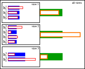
Figure 1: Example of the multiview distributions hierarchy with $3$ views. For all views $v\in\{1,2,3\}$, we have a set of voters ${\cal H}_{v}=\{h_{1}^{v},\ldots,h_{n_{v}}^{v}\}$ on which we consider prior $P_{v}$ view-specific distribution (in blue), and we consider a hyper-prior $\pi$ distribution (in green) over the set of $3$ views. The objective is to learn a posterior $Q_{v}$ (in red) view-specific distributions and a hyper-posterior $\rho$ distribution (in orange) leading to a good model. The length of a rectangle represents the weight (or probability) assigned to a voter or a view.

To tackle multiview learning in a PAC-Bayesian fashion, we propose to define a two-level hierarchy of prior and posterior distributions over the views: i) for each view $v$, we consider a prior $P_{v}$ and a posterior $Q_{v}$ distributions over view-specific voters to capture view-specific information and ii) a hyper-prior $\pi_{v}$ and a hyper-posterior $\rho_{v}$ distributions over the set of views to capture the accuracy of view-specific classifiers and diversity between the views (see Figure 1). Following this distributions’ hierarchy, we define a multiview majority vote classifier where view-specific classifiers are weighted according to posterior and hyper-posterior distributions. By doing so, we extend the classical PAC-Bayesian theory to multiview learning with more than two views and derive a PAC-Bayesian generalization bound for our multiview majority vote classifier.

From a practical point of view, we design an algorithm based on the idea of boosting Freund [1995], Freund and Schapire [1997], Schapire [1999, 2003]. Our boosting-based multiview learning algorithm, called PB-MVBoost, deals with the two-level hierarchical learning strategy. PB-MVBoost is an ensemble method and outputs a multiview classifier that is a combination of view-specific voters. It is well known that controlling the diversity between the view-specific classifiers or the views is a key element in multiview learning Amini et al. [2009], Goyal et al. [2017], Chapelle et al. [2010], Kuncheva [2004], Maillard and Vayatis [2009], Morvant et al. [2014]. Therefore, to learn the weights over the views, we minimize an upper-bound on the error of the majority vote, called the multiview C-bound Germain et al. [2015], Roy et al. [2016], Goyal et al. [2017], allowing us to control a trade-off between accuracy and diversity. Concretely, at each iteration of our multiview algorithm, we learn i) weights over view-specific voters based on their ability to deal with examples on the corresponding view (capturing view-specific informations); and ii) weights over views by minimizing the multiview C-bound. To show the potential of our algorithm, we empirically evaluate our approach on MNIST₁, MNIST₂ and Reuters RCV1/RCV2 collectionsLecun et al. [1998], Amini et al. [2009]. We observe that our algorithm PB-MVBoost, empirically minimizes the multiview C-Bound over iterations, and lead to good performances even when the classes are unbalanced. We compare PB-MVBoost with a previously developed multiview algorithm, denoted by Fusion${}_{\mathtt{all}}^{\mathtt{Cq}}$ Goyal et al. [2017], which first learns the view-specific voters at the base level of the hierarchy, and then, combines the predictions of view-specific voters using a PAC-Bayesian algorithm CqBoost Roy et al. [2016]. From the experimental results, it came out that PB-MVBoost is more stable across different datasets and computationally faster than Fusion${}_{\mathtt{all}}^{\mathtt{Cq}}$.

In the next section, we discuss some related works. In Section 3, we present the PAC-Bayesian multiview learning framework Goyal et al. [2017]. In Section 4, we derive our multiview learning algorithm PB-MVBoost. Before concluding in Section 6, we experiment our algorithm in Section 5.

2 Related Work

Learning a weighted majority vote is closely related to ensemble methods Dietterich [2000], Re and Valentini [2012]. In the ensemble methods literature, it is well known that we desire to combine voters that make errors on different data points Kuncheva [2004]. Intuitively, this means that the voters disagree on some data points. This notion of disagreement (or agreement) is sometimes called diversity between classifiers D ez-Pastor et al. [2015], Brown and Kuncheva [2010], Kuncheva [2004]. Even if there is no consensus on the definition of “diversity”, controlling it while keeping good accuracy is at the heart of a majority of ensemble methods: indeed if all the voters agree on all the points then there is no interest to combine them, only one will be sufficient. Similarly, when we combine multiple views (or representations), it is known that controlling diversity between the views plays a vital role for learning the final majority vote Amini et al. [2009], Goyal et al. [2017], Chapelle et al. [2010], Maillard and Vayatis [2009]. Most of the existing ensemble-based multiview learning algorithms try to exploit either view consistency (agreement between views) Janodet et al. [2009], Koço and Capponi [2011], Xiao and Guo [2012] or diversity between views Xu and Sun [2010], Goyal et al. [2017], Peng et al. [2011, 2017] in different manners. Janodet et al. [2009] proposed a boosting based multiview learning algorithm for 2 views, called 2-Boost. At each iteration, the algorithm learns the weights over the view-specific voters by maintaining a single distribution over the learning examples. Conversely, Koço and Capponi [2011] proposed Mumbo that maintains separate distributions for each view. For each view, the algorithm reduces the weights associated with the examples hard to classify, and increases the weights of those examples in the other views. This trick allows a communication between the views with the objective to maintain view consistency. Compared to our approach, we follow a two-level learning strategy where we learn (hyper-)posterior distributions/weights over view-specific voters and views. In order to take into account accuracy and diversity between the views, we optimize the multiview C-Bound (an upper-bound over the risk of multiview majority vote learned, see e.g.  Germain et al. [2015], Roy et al. [2016], Goyal et al. [2017]).

Xu and Sun [2010] proposed EMV-AdaBoost, an embedded multiview Adaboost algorithm, restricted to two views. At each iteration, an example contributes to the error if it is misclassified by any of the view-specific voters and the diversity between the views is captured by weighting the error by the agreement between the views. Peng et al. [2011, 2017] proposed variants of Boost.SH (boosting with SHared weight distribution) which controls the diversity for more than two views. Similarly than our approach, they maintain a single global distribution over the learning examples for all the views. To control the diversity between the views, at each iteration they update the distribution over the views by casting the algorithm in two ways: i) a multiarmed bandit framework (rBoost.SH) and ii) an expert strategy framework (eBoost.SH) consisting of set of strategies (distribution over views) for weighing views. At the end, their multiview majority vote is a combination of $T$ weighted base voters, where $T$ is the number of iterations for boosting. Whereas, our multiview majority vote is a weighted combination of the view-specific voters over all the weighted views.

Furthermore, our approach encompasses the one of Amini et al. [2009] and Xiao and Guo [2012]. Amini et al. [2009] proposed a Rademacher analysis for expectation of individual risks of each view-specific classifier (for more than two views). Xiao and Guo [2012] derived a weighted majority voting Adaboost algorithm which learns weights over view-specific voters at each iteration of the algorithm. Both of these approaches maintain a uniform distribution over the views whereas our algorithm learns the weights over the views such that they capture diversity between the views. Moreover, it is important to note that Sun et al. [2017] proposed a PAC-Bayesian analysis for multiview learning over the concatenation of views but limited to two views and to a particular kind of voters: linear classifiers. This has allowed them to derive a SVM-like learning algorithm but dedicated to multiview with exactly two views. In our work, we are interested in learning from more than two views and no restriction on the classifier type. Contrary to them, we followed a two-level distributions’ hierarchy where we learn weights over view-specific classifiers and weights over views.

3 The Multiview PAC-Bayesian Framework

3.1 Notations and Setting

In this work, we tackle multiview binary classification tasks where the observations are described with $V\geq 2$ different representation spaces, i.e., views; let ${\cal V}$ be the set of these $V$ views. Formally, we focus on tasks for which the input space is ${\cal X}={\cal X}_{1}\times\dots\times{\cal X}_{V}$, where $\forall v\in{\cal V},\ X_{v}\subseteq\mathbb{R}^{d_{v}}$ is a $d_{v}$-dimensional input space, and the binary output space is ${\cal Y}=\{-1,+1\}$. We assume that ${\cal D}$ is an unknown distribution over ${\cal X}\times{\cal Y}$. We stand in the PAC-Bayesian supervised learning setting where an observation $\mathbf{x}=(x^{1},x^{2},\dots,x^{V})\in{\cal X}$ is given with its label $y\in{\cal Y}$, and is independently and identically drawn (i.i.d.) from ${\cal D}$. A learning algorithm is then provided with a training sample $S$ of $n$ examples i.i.d. from ${\cal D}$: $S=\{(\mathbf{x}_{i},y_{i})\}_{i=1}^{n}\sim({\cal D})^{n}$, where $({\cal D})^{n}$ stands for the distribution of a $n$-sample. For each view $v\in{\cal V}$, we consider a view-specific set ${\cal H}_{v}$ of voters $h:\mathcal{X}_{v}\to{\cal Y}$, and a prior distribution $P_{v}$ on ${\cal H}_{v}$. Given a hyper-prior distribution $\pi$ over the views ${\cal V}$, and a multiview learning sample $S$, our PAC-Bayesian learner objective is twofold: i) finding a posterior distribution $Q_{v}$ over $\mathcal{H}_{v}$ for all views $v\in{\cal V}$; ii) finding a hyper-posterior distribution $\rho$ on the set of the views ${\cal V}$. This defines a hierarchy of distributions illustrated on Figure 1. The learned distributions express a multiview weighted majority vote defined as

$$B_{\rho}(\mathbf{x})=\operatorname{sign}\left[{\displaystyle\operatorname*{\mathbb{E}}_{v\sim\rho}}\ {\displaystyle\operatorname*{\mathbb{E}}_{h\sim Q_{v}}}h(x^{v})\right].$$ (1)

Thus, the learner aims at constructing the posterior and hyper-posterior distributions that minimize the true risk $R_{\mathcal{D}}(B_{\rho})$ of the multiview weighted majority vote

$$R_{\mathcal{D}}(B_{\rho})={\displaystyle\operatorname*{\mathbb{E}}_{(\mathbf{x},y)\sim\mathcal{D}}}\mathds{1}_{[B_{\rho}(\mathbf{x})\neq y]},$$

where $\mathds{1}_{[\pi]}=1$ if the predicate $\pi$ is true and $0$ otherwise. The above risk of the deterministic weighted majority vote is closely related to the Gibbs risk $R_{{\cal D}}(G_{\rho})$ defined as the expectation of the individual risks of each voter that appears in the majority vote. More formally, in our multiview setting, we have

$$R_{\mathcal{D}}(G_{\rho})\ =\ {\displaystyle\operatorname*{\mathbb{E}}_{({\bf x},y)\sim{\cal D}}}\ {\displaystyle\operatorname*{\mathbb{E}}_{v\sim\rho}}\ {\displaystyle\operatorname*{\mathbb{E}}_{h\sim Q_{v}}}\mathds{1}_{[h(x^{v})\neq y]},$$

and its empirical counterpart is

$$R_{S}(G_{\rho}) =\frac{1}{n}\sum_{i=1}^{n}{\displaystyle\operatorname*{\mathbb{E}}_{v\sim\rho}}\ {\displaystyle\operatorname*{\mathbb{E}}_{h\sim Q_{v}}}\mathds{1}_{[h(x_{i}^{v})\neq y_{i}]}.$$

In fact, if $B_{\rho}$ misclassifies ${\bf x}\in{\cal X}$, then at least half of the view-specific voters from all the views (according to hyper-posterior and posterior distributions) makes an error on ${\bf x}$. Then, it is well known (e.g., Shawe-Taylor and Langford [2003], McAllester [2003], Germain et al. [2015]) that $R_{{\cal D}}(B_{\rho})$ is upper-bounded by twice $R_{{\cal D}}(G_{\rho})$:

$$R_{\mathcal{D}}(B_{\rho})\leq 2R_{\mathcal{D}}(G_{\rho}).$$

In consequence, a generalization bound for $R_{\mathcal{D}}(G_{\rho})$ gives rise to a generalization bound for $R_{\mathcal{D}}(B_{\rho})$.

There exist other tighter relations Langford and Shawe-Taylor [2002], Lacasse et al. [2006], Germain et al. [2015], such as the C-Bound Lacasse et al. [2006], Germain et al. [2015] which captures a trade-off between the Gibbs risk $R_{\mathcal{D}}(G_{\rho})$ and the disagreement between pairs of voters. This latter can be seen as a measure of diversity among the voters involved in the majority vote Roy et al. [2011], Morvant et al. [2014], that is a key element to control from a multiview point of view Amini et al. [2009], Atrey et al. [2010], Kuncheva [2004], Maillard and Vayatis [2009], Goyal et al. [2017]. The C-Bound can be extended to our multiview setting as below.

Lemma 1 (Multiview C-Bound)

Let $V\geq 2$ be the number of views. For all posterior $\{Q_{v}\}_{v=1}^{V}$ distributions over $\{{\cal H}_{v}\}_{v=1}^{V}$ and hyper-posterior $\rho$ distribution over views $\mathcal{V}$, if $R_{{\cal D}}(G_{\rho})<\frac{1}{2}$, then we have

$$R_{\mathcal{D}}(B_{\rho}) \leq 1-\frac{\displaystyle\big{(}1-2R_{{\cal D}}(G_{\rho})\big{)}^{2}}{\displaystyle 1-2d_{{\cal D}}(\rho)}$$ (2)

$$\leq 1-\frac{\Big{(}1-2\operatorname*{\mathbb{E}}_{v\sim\rho}R_{{\cal D}}(G_{Q_{v}})\Big{)}^{2}}{1-2\operatorname*{\mathbb{E}}_{v\sim\rho}d_{{\cal D}}(Q_{v})}\,,$$ (3)

where $d_{{\cal D}}(\rho)$ is the expected disagreement between pairs of voters defined as

$$d_{{\cal D}}(\rho)\ =\ \operatorname*{\mathbb{E}}_{{\bf x}\sim\mathcal{D}_{\mathcal{X}}}\operatorname*{\mathbb{E}}_{v\sim\rho}\operatorname*{\mathbb{E}}_{v^{\prime}\sim\rho}\operatorname*{\mathbb{E}}_{h\sim Q_{v}}\operatorname*{\mathbb{E}}_{h^{\prime}\sim Q_{v^{\prime}}}\mathds{1}_{[h(x^{v}){\neq}h^{\prime}(x^{v^{\prime}})]},$$

and $R_{\cal D}(G_{Q_{v}})$ and $d_{{\cal D}}(Q_{v})$ are respectively the true view-specific Gibbs risk and the expected disagreement defined as

$$R_{\mathcal{D}}(G_{Q_{v}}) ={\displaystyle\operatorname*{\mathbb{E}}_{({\bf x},y)\sim{\cal D}}}\ {\displaystyle\operatorname*{\mathbb{E}}_{h\sim Q_{v}}}\mathds{1}_{[h(x^{v})\neq y]}\,,$$

$$d_{{\cal D}}(Q_{v}) =\operatorname*{\mathbb{E}}_{{\bf x}\sim\mathcal{D}_{\mathcal{X}}}\operatorname*{\mathbb{E}}_{h\sim Q_{v}}\operatorname*{\mathbb{E}}_{h^{\prime}\sim Q_{v}}\mathds{1}_{[h(x^{v}){\neq}h^{\prime}(x^{v})]}.$$

Proof.  Similarly than done for the classical C-Bound Lacasse et al. [2006], Germain et al. [2015], Equation (2) follows from the Cantelli-Chebyshev’s inequality (we provide the proof in B).
Equation (3) is obtained by rewriting $R_{\mathcal{D}}(G_{\rho})$ as the $\rho$-average of the risk associated to each view, and the lower-bounding $d_{{\cal D}}(\rho)$ by the $\rho$-average of the disagreement associated to each view. First we notice that in the binary setting where $y\in\{-1,1\}$ and $h:{\cal X}\to\{-1,1\}$, we have $\mathds{1}_{[h(x^{v})\neq y]}=\frac{1}{2}(1-y\,h(x^{v}))$, and

$$R_{\mathcal{D}}(G_{\rho})\ =\ {\displaystyle\operatorname*{\mathbb{E}}_{(\mathbf{x},y)\sim\mathcal{D}}}\ {\displaystyle\operatorname*{\mathbb{E}}_{v\sim\rho}}\ {\displaystyle\operatorname*{\mathbb{E}}_{h\sim Q_{v}}}\mathds{1}_{[h(x^{v})\neq y]}$$

$$=\ \frac{1}{2}\bigg{(}1-{\displaystyle\operatorname*{\mathbb{E}}_{({\bf x},y)\sim\mathcal{D}}}\ {\displaystyle\operatorname*{\mathbb{E}}_{v\sim\rho}}\ {\displaystyle\operatorname*{\mathbb{E}}_{h\sim Q_{v}}}y\,h(x^{v})\bigg{)}$$

$$=\ {\displaystyle\operatorname*{\mathbb{E}}_{v\sim\rho}}R_{\mathcal{D}}(G_{Q_{v}})\,.$$

Moreover, we have

$$d_{{\cal D}}(\rho)\ =\ \operatorname*{\mathbb{E}}_{{\bf x}\sim\mathcal{D}_{\mathcal{X}}}\operatorname*{\mathbb{E}}_{v\sim\rho}\operatorname*{\mathbb{E}}_{v^{\prime}\sim\rho}\operatorname*{\mathbb{E}}_{h\sim Q_{v}}\operatorname*{\mathbb{E}}_{h^{\prime}\sim Q_{v^{\prime}}}\mathds{1}_{[h(x^{v}){\neq}h^{\prime}(x^{v^{\prime}})]}$$

$$=\ \frac{1}{2}\bigg{(}1-\operatorname*{\mathbb{E}}_{{\bf x}\sim\mathcal{D}_{\mathcal{X}}}\operatorname*{\mathbb{E}}_{v\sim\rho}\operatorname*{\mathbb{E}}_{v^{\prime}\sim\rho}\operatorname*{\mathbb{E}}_{h\sim Q_{v}}\operatorname*{\mathbb{E}}_{h\sim Q_{v^{\prime}}}h(x^{v})\times h^{\prime}(x^{v^{\prime}})\bigg{)}$$

$$=\ \frac{1}{2}\bigg{(}1-{\displaystyle\operatorname*{\mathbb{E}}_{{\bf x}\sim\mathcal{D}_{\mathcal{X}}}}\bigg{[}{\displaystyle\operatorname*{\mathbb{E}}_{v\sim\rho}}\,{\displaystyle\operatorname*{\mathbb{E}}_{h\sim Q_{v}}}h(x^{v})\bigg{]}^{2}\bigg{)}\,.$$

From Jensen’s inequality (Theorem 4, in Appendix) it comes

$$d_{{\cal D}}(\rho)\ \geq\ \frac{1}{2}\bigg{(}1-{\displaystyle\operatorname*{\mathbb{E}}_{{\bf x}\sim\mathcal{D}_{\mathcal{X}}}}\,{\displaystyle\operatorname*{\mathbb{E}}_{v\sim\rho}}\bigg{[}{\displaystyle\operatorname*{\mathbb{E}}_{h\sim Q_{v}}}h(x^{v})\bigg{]}^{2}\bigg{)}$$

$$=\ {\displaystyle\operatorname*{\mathbb{E}}_{v\sim\rho}}\Bigg{[}\frac{1}{2}\bigg{(}1-{\displaystyle\operatorname*{\mathbb{E}}_{{\bf x}\sim\mathcal{D}_{\mathcal{X}}}}\bigg{[}{\displaystyle\operatorname*{\mathbb{E}}_{h\sim Q_{v}}}h(x^{v})\bigg{]}^{2}\bigg{)}\Bigg{]}$$

$$=\ {\displaystyle\operatorname*{\mathbb{E}}_{v\sim\rho}}d_{{\cal D}}(Q_{v})\,.$$

By replacing $R_{\mathcal{D}}(G_{\rho})$ and $d_{{\cal D}}(\rho)$ in Equation (2), we obtain

$$1-\frac{\displaystyle\big{(}1-2R_{{\cal D}}(G_{\rho})\big{)}^{2}}{\displaystyle 1-2d_{{\cal D}}(\rho)}\leq 1-\frac{\Big{(}1-2\operatorname*{\mathbb{E}}_{v\sim\rho}R_{{\cal D}}(G_{Q_{v}})\Big{)}^{2}}{1-2\operatorname*{\mathbb{E}}_{v\sim\rho}d_{{\cal D}}(Q_{v})}\,.$$

 

Equation (2) suggests that a good trade-off between the Gibbs risk and the disagreement between pairs of voters will lead to a well-performing majority vote. Equation (3) controls the diversity among the views (important for multiview learning Amini et al. [2009], Goyal et al. [2017], Chapelle et al. [2010], Maillard and Vayatis [2009]) thanks to the disagreement’s expectation over the views $\operatorname*{\mathbb{E}}_{v\sim\rho}d_{{\cal D}}(Q_{v})$.

3.2 The General Multiview PAC-Bayesian Theorem

In this section, we give a general multiview PAC-Bayesian theorem Goyal et al. [2017] that takes the form of a generalization bound for the Gibbs risk in the context of a two-level hierarchy of distributions. A key step in PAC-Bayesian proofs is the use of a change of measure inequality [McAllester, 2003], based on the Donsker-Varadhan inequality [Donsker and Varadhan, 1975]. Lemma 2 below extends this tool to our multiview setting.

Lemma 2

For any set of priors $\{P_{v}\}_{v=1}^{V}$ over $\{{\cal H}_{v}\}_{v=1}^{V}$ and any set of posteriors $\{Q_{v}\}_{v=1}^{V}$ over $\{{\cal H}_{v}\}_{v=1}^{V}$, for any hyper-prior distribution $\pi$ on views ${\cal V}$ and hyper-posterior distribution $\rho$ on ${\cal V}$, and for any measurable function $\phi:\mathcal{H}_{v}\to\mathbb{R}$, we have

$${\displaystyle\operatorname*{\mathbb{E}}_{v\sim\rho}}\ {\displaystyle\operatorname*{\mathbb{E}}_{h\sim Q_{v}}}\phi(h)\leq\ {\displaystyle\operatorname*{\mathbb{E}}_{v\sim\rho}}\operatorname{KL}(Q_{v}\|P_{v})+\operatorname{KL}(\rho\|\pi)+\ln\left({\displaystyle\operatorname*{\mathbb{E}}_{v\sim\pi}}\ {\displaystyle\operatorname*{\mathbb{E}}_{h\sim P_{v}}}e^{\phi(h)}\right).$$

Proof.  Deferred to C   

Based on Lemma 2, the following theorem gives a generalization bound for multiview learning. Note that, as done by Germain et al. [2009, 2015] we rely on a general convex function $D:[0,1]\times[0,1]\to\mathbb{R}$, which measures the “deviation” between the empirical and the true Gibbs risk.

Theorem 1

Let $V\geq 2$ be the number of views. For any distribution ${\cal D}$ on ${\cal X}\times{\cal Y}$, for any set of prior distributions $\{P_{v}\}_{v=1}^{V}$ over $\{{\cal H}_{v}\}_{v=1}^{V}$, for any hyper-prior distributions $\pi$ over ${\cal V}$, for any convex function $D:[0,1]\times[0,1]\to\mathbb{R}$, for any $\delta\in(0,1]$, with a probability at least $1-\delta$ over the random choice of $S\sim({\cal D})^{n}$, for all posterior $\{Q_{v}\}_{v=1}^{V}$ over $\{{\cal H}_{v}\}_{v=1}^{V}$ and hyper-posterior $\rho$ over ${\cal V}$ distributions, we have:

$$D\left(R_{S}(G_{\rho}),R_{\mathcal{D}}(G_{\rho})\right)\leq\frac{1}{m}\bigg{[}{\displaystyle\operatorname*{\mathbb{E}}_{v\sim\rho}}\,\operatorname{KL}(Q_{v}\|P_{v})$$

$$\qquad\qquad\qquad\qquad\qquad+\operatorname{KL}(\rho\|\pi)+\ln\left(\frac{1}{\delta}\,{\displaystyle\operatorname*{\mathbb{E}}_{S\sim({\cal D})^{n}}}\,{\displaystyle\operatorname*{\mathbb{E}}_{v\sim\pi}}\,{\displaystyle\operatorname*{\mathbb{E}}_{h\sim P_{v}}}e^{nD\left(R_{S}(h),R_{\cal D}(h)\right)}\right)\bigg{]}.$$

Proof.  First, note that ${\displaystyle\operatorname*{\mathbb{E}}_{v\sim\pi}}\,{\displaystyle\operatorname*{\mathbb{E}}_{h\sim P_{v}}}e^{nD(R_{S}(h),R_{\cal D}(h))}$ is a non-negative random variable. Using Markov’s inequality, with $\delta\in(0,1]$, and a probability at least $1-\delta$ over the random choice of the multiview learning sample $S\sim({\cal D})^{n}$, we have

$${\displaystyle\operatorname*{\mathbb{E}}_{v\sim\pi}}\ {\displaystyle\operatorname*{\mathbb{E}}_{h\sim P_{v}}}e^{n\,D(R_{S}(h),R_{\cal D}(h))}\leq\ \frac{1}{\delta}{\displaystyle\operatorname*{\mathbb{E}}_{S\sim({\cal D})^{n}}}\ {\displaystyle\operatorname*{\mathbb{E}}_{v\sim\pi}}\ {\displaystyle\operatorname*{\mathbb{E}}_{h\sim P_{v}}}e^{nD(R_{S}(h),R_{\cal D}(h))}.$$

By taking the logarithm on both sides, with a probability at least $1-\delta$ over $S\sim({\cal D})^{n}$, we have

$$\ln\bigg{[}{\displaystyle\operatorname*{\mathbb{E}}_{v\sim\pi}}\ {\displaystyle\operatorname*{\mathbb{E}}_{h\sim P_{v}}}e^{n\,D(R_{S}(h),R_{\cal D}(h))}\bigg{]}\leq\ln\bigg{[}\frac{1}{\delta}{\displaystyle\operatorname*{\mathbb{E}}_{S\sim({\cal D})^{n}}}\ {\displaystyle\operatorname*{\mathbb{E}}_{v\sim\pi}}\ {\displaystyle\operatorname*{\mathbb{E}}_{h\sim P_{v}}}e^{nD(R_{S}(h),R_{\cal D}(h))}\bigg{]}$$ (4)

We now apply Lemma 2 on the left-hand side of the Inequality (4) with $\phi(h)=n\,D(R_{S}(h),R_{\cal D}(h))$. Therefore, for any $Q_{v}$ on $\mathcal{H}_{v}$ for all views $v\in{\cal V}$, and for any $\rho$ on views ${\cal V}$, with a probability at least $1-\delta$ over $S\sim({\cal D})^{n}$, we have

$$\ln\bigg{[}\underset{v\sim\pi}{\mathbb{E}}\ \underset{h\sim P_{v}}{\mathbb{E}}e^{n\,D(R_{S}(h),R_{\cal D}(h))}\bigg{]}$$

$$\geq\ n\,\underset{v\sim\rho}{\mathbb{E}}\ \underset{h\sim Q_{v}}{\mathbb{E}}D(R_{S}(h),R_{\cal D}(h))-\underset{v\sim\rho}{\mathbb{E}}\ \operatorname{KL}(Q_{v}\|P_{v})-\operatorname{KL}(\rho\|\pi)$$

$$\geq\ n\,D\left(\underset{v\sim\rho}{\mathbb{E}}\ \underset{h\sim Q_{v}}{\mathbb{E}}R_{S}(h),\underset{v\sim\rho}{\mathbb{E}}\ \underset{h\sim Q_{v}}{\mathbb{E}}R_{\cal D}(h)\right)-\underset{v\sim\rho}{\mathbb{E}}\ \operatorname{KL}(Q_{v}\|P_{v})-\operatorname{KL}(\rho\|\pi),$$

where the last inequality is obtained by applying Jensen’s inequality on the convex function $D$. By rearranging the terms, we have

$$D\left(\underset{v\sim\rho}{\mathbb{E}}\ \underset{h\sim Q_{v}}{\mathbb{E}}R_{S}(h),\underset{v\sim\rho}{\mathbb{E}}\ \underset{h\sim Q_{v}}{\mathbb{E}}R_{\cal D}(h)\right)\, \leq\,\frac{1}{m}\bigg{[}\underset{v\sim\rho}{\mathbb{E}}\ \operatorname{KL}(Q_{v}\|P_{v})+\operatorname{KL}(\rho\|\pi)$$

$$+\ln\bigg{(}\frac{1}{\delta} \underset{S\sim({\cal D})^{n}}{\mathbb{E}}\ \underset{v\sim\pi}{\mathbb{E}}\ \underset{h\sim P_{v}}{\mathbb{E}}e^{n\,D\left(R_{S}(h),R_{\cal D}(h)\right)}\bigg{)}\bigg{]}$$

Finally, the theorem statement is obtained by rewriting

$$\operatorname*{\mathbb{E}}_{v\sim\rho}\operatorname*{\mathbb{E}}_{h\sim Q_{v}}R_{S}(h) =R_{S}(G_{\rho}),$$ (5)

$$\operatorname*{\mathbb{E}}_{v\sim\rho}\operatorname*{\mathbb{E}}_{h\sim Q_{v}}R_{\cal D}(h) =R_{\cal D}(G_{\rho})\,.$$ (6)

 

Compared to the classical single-view PAC-Bayesian Bound of Germain et al. [2009, 2015], the main difference relies on the introduction of the view-specific prior and posterior distributions, which mainly leads to an additional term $\mathbf{E}_{v\sim\rho}\operatorname{KL}(Q_{v}\|P_{v})$ expressed as the expectation of the view-specific Kullback-Leibler divergence term over the views ${\cal V}$ according to the hyper-posterior distribution $\rho$.

Theorem 1 provides tools to derive PAC-Bayesian generalization bounds for a multiview supervised learning setting. Indeed, by making use of the same trick as Germain et al. [2009, 2015], by choosing a suitable convex function $D$ and upper-bounding ${\displaystyle\operatorname*{\mathbb{E}}_{S\sim({\cal D})^{n}}}\ {\displaystyle\operatorname*{\mathbb{E}}_{v\sim\pi}}{\displaystyle\operatorname*{\mathbb{E}}_{h\sim P_{v}}}e^{n\,D(R_{S}(h),R_{\cal D}(h))}$, we obtain instantiation of Theorem 1 . In the next section we give an example of this kind of deviation through the approach of Catoni [2007], that is one of the three classical PAC-Bayesian Theorems Catoni [2007], McAllester [1999], Seeger [2002], Langford [2005].

3.3 An Example of Instantiation of the Multiview PAC-Bayesian Theorem

To obtain the following theorem which is a generalization bound with the Catoni [2007]’s point of view, we put $D$ as $D(a,b)=\mathcal{F}(b)-C\,a$ where $\cal F$ is a convex function ${\cal F}$ and $C>0$ is a real number [Germain et al., 2009, 2015].

Corollary 1

Let $V\geq 2$ be the number of views. For any distribution $\mathcal{D}$ on ${\cal X}\times{\cal Y}$, for any set of prior distributions $\{P_{v}\}_{v=1}^{V}$ on $\{{\cal H}\}_{v=1}^{V}$, for any hyper-prior distributions $\pi$ over ${\cal V}$, for any $\delta\in(0,1]$, with a probability at least $1-\delta$ over the random choice of $S\sim({\cal D})^{n}$ for all posterior $\{Q_{v}\}_{v=1}^{V}$ and hyper-posterior $\rho$ distributions, we have:

$$R_{\mathcal{D}}(G_{\rho})$$

$$\leq \frac{1}{1\!-\!e^{-C}}\Bigg{(}\!1-\!\exp\bigg{[}-\!\!\bigg{(}C\,R_{S}(G_{\rho})+\frac{1}{n}\Big{[}{\displaystyle\operatorname*{\mathbb{E}}_{v\sim\rho}}\operatorname{KL}(Q_{v}\|P_{v})+\operatorname{KL}(\rho\|\pi)+\ln\tfrac{1}{\delta}\Big{]}\bigg{)}\bigg{]}\Bigg{)}.$$

Proof.  Deferred to D.   

This bound has the advantage of expressing a trade-off between the empirical Gibbs risk and the Kullback-Leibler divergences.

3.4 A Generalization Bound for the C-Bound

From a practical standpoint, as pointed out before, controlling the multiview C-Bound of Equation (3) can be very useful for tackling multiview learning. The next theorem is a generalization bound that justify the empirical minimization of the multiview C-bound (we use in our algorithm PB-MVBoost derived in Section 4).

Theorem 2

Let $V\geq 2$ be the number of views. For any distribution ${\cal D}$ on ${\cal X}\times{\cal Y}$, for any set of prior distributions $\{P_{v}\}_{v=1}^{V}$, for any hyper-prior distributions $\pi$ over views ${\cal V}$, and for any convex function $D:[0,1]\times[0,1]\to\mathbb{R}$, with a probability at least $1-\delta$ over the random choice of $S\sim(D)^{n}$ for all posterior $\{Q_{v}\}_{v=1}^{v}$ and hyper-posterior $\rho$ distributions, we have:

$$R_{\mathcal{D}}(B_{\rho})\leq 1-\frac{\bigg{(}1-2{\displaystyle\operatorname*{\mathbb{E}}_{v\sim\rho}}\mathtt{sup}\ \big{(}\mathbf{r}_{Q_{v},\mathcal{S}}^{\delta/2}\big{)}\bigg{)}^{2}}{1-2{\displaystyle\operatorname*{\mathbb{E}}_{v\sim\rho}}\mathtt{inf}\ \mathbf{d}_{Q_{v},\mathcal{S}}^{\delta/2}}\,,$$

where

$$\mathbf{r}_{Q_{v},\mathcal{S}}^{\delta/2} =\bigg{\{}r:\operatorname{kl}(R_{S}(Q_{v})\|r)\leq\frac{1}{n}\bigg{[}\operatorname{KL}(Q_{v}\|P_{v})+\ln\frac{4\sqrt{m}}{\delta}\bigg{]}\mbox{ and }r\leq\frac{1}{2}\bigg{\}}$$ (7)

$$\mbox{and}\quad\mathbf{d}_{Q_{v},\mathcal{S}}^{\delta/2} =\bigg{\{}d:\operatorname{kl}(d_{Q_{v}}^{S}\|d)\leq\frac{1}{n}\bigg{[}2.\operatorname{KL}(Q_{v}\|P_{v})+\ln\frac{4\sqrt{m}}{\delta}\bigg{]}\bigg{\}}$$ (8)

Proof.  Similarly to Equations $(23)$ and $(24)$ of Germain et al. [2015], we define the sets $\mathbf{r}_{Q_{v},\mathcal{S}}^{\delta/2}$ (Equation (7)) and $\mathbf{d}_{Q_{v},\mathcal{S}}^{\delta/2}$ (Equation (8)) for our setting. Finally, the bound is obtained (from Equation (3) of Lemma 1) by replacing the view-specific Gibbs risk $R_{{\cal D}}(G_{Q_{v}})$ by its upper bound $\mathtt{sup}\ \mathbf{r}_{Q_{v},\mathcal{S}}^{\delta/2}$ and expected disagreement $d_{{\cal D}}(Q_{v})$ by its lower bound $\mathtt{inf}\ \mathbf{d}_{Q_{v},\mathcal{S}}^{\delta/2}$.   

4 The PB-MVBoost algorithm

Algorithm 1 PB-MVBoost

Input: Training set $S=(\mathbf{x}_{i},y_{i}),\dots,(\mathbf{x}_{n},y_{n})$, where $\mathbf{x}_{i}=(x^{1},x^{2},\dots,x^{V})$ and $y_{i}\in\{-1,1\}$.
             For each view $v\in\mathcal{V}$, a view-specific hypothesis set $\mathcal{H}_{v}$.
             Number of iterations $T$.

1:for $\mathbf{x}_{i}\in S$ do

2:     ${\cal D}_{1}(\mathbf{x}_{i})\leftarrow\frac{1}{n}$

3:$\forall v\in{\cal V}$ $\rho_{v}^{1}\leftarrow\frac{1}{V}$

4:for $t=1,\dots,T$ do

5:     $\forall v\in{\cal V},\ h_{v}^{t}\leftarrow\operatorname*{\mathrm{argmin}}_{h\in{\cal H}_{v}}{\displaystyle\operatorname*{\mathbb{E}}_{(\mathbf{x}_{i},y_{i})\sim{\cal D}_{t}}}\left[\mathds{1}_{[h(x_{i}^{v})\neq y_{i}]}\right]$

6:     Compute error: $\forall v\in{\cal V},\ \epsilon_{v}^{t}\leftarrow{\displaystyle\operatorname*{\mathbb{E}}_{(\mathbf{x}_{i},y_{i})\sim{\cal D}_{t}}}\left[\mathds{1}_{[h_{v}^{t}(x_{i}^{v})\neq y_{i}]}\right]$

7:     Compute voter weights (taking into account view specific information):

$$\forall v\in{\cal V},Q_{v}^{t}\leftarrow\frac{1}{2}\bigg{[}\ln\bigg{(}\frac{1-\epsilon_{v}^{t}}{\epsilon_{v}^{t}}\bigg{)}\bigg{]}$$

8:     Optimize the multiview C-Bound to learn weights over the views

$$\mathrm{max}_{\rho} \qquad\frac{\bigg{[}1-2\sum_{v=1}^{V}\rho_{v}^{t}r_{v}^{t}\bigg{]}^{2}}{1-2\sum_{v=1}^{V}\rho_{v}^{t}d_{v}^{t}}$$

$$s.t. \qquad\sum_{v=1}^{V}\rho_{v}^{t}=1,\quad\rho_{v}^{t}\geq 0\quad\forall v\in\{1,...,V\}$$

where $$\forall v\in{\cal V},\ r_{v}^{t}\leftarrow{\displaystyle\operatorname*{\mathbb{E}}_{(\mathbf{x}_{i},y_{i})\sim{\cal D}_{t}}}\ {\displaystyle\operatorname*{\mathbb{E}}_{h\sim\mathcal{H}_{v}}}\left[\mathds{1}_{[h(x_{i}^{v})\neq y_{i}]}\right]$$

$$\forall v\in{\cal V},\ d_{v}^{t}\leftarrow{\displaystyle\operatorname*{\mathbb{E}}_{(\mathbf{x}_{i},y_{i})\sim{\cal D}_{t}}}\ {\displaystyle\operatorname*{\mathbb{E}}_{h,h^{\prime}\sim\mathcal{H}_{v}}}\left[\mathds{1}_{[h(x_{i}^{v})\neq h^{\prime}(x_{i}^{v})]}\right]$$

9:     for $\mathbf{x}_{i}\in S$ do

10:         ${\cal D}_{t+1}(\mathbf{x}_{i})\leftarrow\frac{{\cal D}_{t}(\mathbf{x}_{i})\exp\big{(}{-y_{i}\sum_{v=1}^{V}\rho_{v}^{t}Q_{v}^{t}h_{v}^{t}(x_{i}^{v})}\big{)}}{\sum_{j=1}^{n}{\cal D}_{t}(\mathbf{x}_{j})\exp\big{(}{-y_{j}\sum_{v=1}^{V}\rho_{v}^{t}Q_{v}^{t}h_{v}^{t}(x_{j}^{v})}\big{)}}$      

11:Return: For each view $v\in{\cal V},$ weights over view-specific voters and weights over views i.e. $\rho^{T}$

Following our two-level hierarchical strategy (see Figure 1), we aim at combining the view-specific voters (or views) leading to a well-performing multiview majority vote given by Equation (1). Boosting is a well-known approach which aims at combining a set of weak voters in order to build a more efficient classifier than each of the view-specific classifiers alone. Typically, boosting algorithms repeatedly learn a “weak” voter using a learning algorithm with different probability distribution over the learning sample $S$. Finally, it combines all the weak voters in order to have one single strong classifier which performs better than the individual weak voters. Therefore, we exploit boosting paradigm to derive a multiview learning algorithm PB-MVBoost (see Algorithm 1) for our setting.

For a given training set $S=\{(\mathbf{x}_{i},y_{i}),\dots,(\mathbf{x}_{n},y_{n})\}\in(\mathcal{X}\times\{-1,+1\})^{n}$ of size $n$; the proposed algorithm (Algorithm 1) maintains a distribution over the examples which is initialized as uniform. Then at each iteration, $V$ view-specific weak classifiers are learned according to the current distribution ${\cal D}_{t}$ (Step 5), and their corresponding errors $\epsilon^{t}_{v}$ are estimated (Step 6).

Similarly to the Adaboost algorithm Freund and Schapire [1997], the weights of each view-specific classifier $(Q_{v}^{t})_{1\leq v\leq V}$ are then computed with respect to these errors as

$$\forall v\in{\cal V},Q_{v}^{t}\leftarrow\frac{1}{2}\bigg{[}\ln\bigg{(}\frac{1-\epsilon_{v}^{t}}{\epsilon_{v}^{t}}\bigg{)}\bigg{]}$$

To learn the weights $(\rho_{v})_{1\leq v\leq V}$ over the views, we optimize the multiview C-Bound, given by Equation (3) of Lemma 1 (Step 8 of algorithm), which in our case writes as a constraint minimization problem

$$\mathrm{max}_{\rho} \qquad\frac{\bigg{[}1-2\sum_{v=1}^{V}\rho_{v}^{t}r_{v}^{t}\bigg{]}^{2}}{1-2\sum_{v=1}^{V}\rho_{v}^{t}d_{v}^{t}}$$

$$s.t. \qquad\sum_{v=1}^{V}\rho_{v}^{t}=1,\quad\rho_{v}^{t}\geq 0\quad\forall v\in\{1,...,V\}$$

where, $r_{v}$ is the view-specific Gibbs risk and, $d_{v}$ the expected disagreement over all view-specific voters defined as follows.

$$\ r_{v}^{t}={\displaystyle\operatorname*{\mathbb{E}}_{(\mathbf{x}_{i},y_{i})\sim{\cal D}_{t}}}\ {\displaystyle\operatorname*{\mathbb{E}}_{h\sim\mathcal{H}_{v}}}\mathds{1}_{[h(x_{i}^{v})\neq y_{i}]},$$ (9)

$$\ d_{v}^{t}={\displaystyle\operatorname*{\mathbb{E}}_{(\mathbf{x}_{i},y_{i})\sim{\cal D}_{t}}}\ {\displaystyle\operatorname*{\mathbb{E}}_{h,h^{\prime}\sim\mathcal{H}_{v}}}\mathds{1}_{[h(x_{i}^{v})\neq h^{\prime}(x_{i}^{v})]}.$$ (10)

Intuitively, the multiview C-Bound tries to diversify the view-specific voters and views (Equation (10)) while controlling the classification error of the view-specific classifiers (Equation (9)). This allows us to control the accuracy and the diversity between the views which is an important ingredient in multiview learning Xu and Sun [2010], Goyal et al. [2017], Peng et al. [2011, 2017], Morvant et al. [2014].

In Section 5, we empirically show that our algorithm minimizes the multiview C-Bound over the iterations of the algorithm (this is theoretically justified by the generalization bound of Theorem 2). Finally, we update the distribution over training examples $\mathbf{x}_{i}$ (Step 9), by following the Adaboost algorithm and in a way that the weights of misclassified (resp. well classified) examples by the final weighted majority classifier increase (resp. decrease).

$${\cal D}_{t+1}(\mathbf{x}_{i})\leftarrow\frac{{\cal D}_{t}(\mathbf{x}_{i})\exp\big{(}{-y_{i}\sum_{v=1}^{V}\rho_{v}^{t}Q_{v}^{t}h_{v}^{t}(x_{i}^{v})}\big{)}}{\sum_{j=1}^{n}{\cal D}_{t}(\mathbf{x}_{j})\exp\big{(}{-y_{j}\sum_{v=1}^{V}\rho_{v}^{t}Q_{v}^{t}h_{v}^{t}(x_{j}^{v})}\big{)}}$$

Intuitively, this forces the view-specific classifiers to be consistent with each other, which is important for multiview learning Janodet et al. [2009], Koço and Capponi [2011], Xiao and Guo [2012]. Finally, after $T$ iterations of algorithm, we learn the weights over the view-specific voters and weights over the views leading to a well-performing weighted multiview majority vote

$$B_{\rho}(\mathbf{x})=\operatorname{sign}\left(\sum_{v=1}^{V}\rho_{v}^{T}\sum_{t=1}^{T}Q_{v}^{t}h_{v}^{t}(x^{v})\right).$$

5 Experimental Results

In this section, we present experiments to show the potential of our algorithm PB-MVBoost on the following datasets.

5.1 Datasets

MNIST

MNIST is a publicly available dataset consisting of $70,000$ images of handwritten digits distributed over ten classes Lecun et al. [1998]. For our experiments, we generated $2$ four-view datasets where each view is a vector of $\mathbb{R}^{14\times 14}$. Similarly than done by  Chen and Denoyer [2017], the first dataset ($\mathtt{MNIST}_{1}$) is generated by considering $4$ quarters of image as $4$ views. For the second dataset ($\mathtt{MNIST}_{2}$) we consider $4$ overlapping views around the centre of images: this dataset brings redundancy between the views. These two datasets allow us to check if our algorithm is able to capture redundancy between the views. We reserve $10,000$ of images as test samples and remaining as training samples.

Multilingual, Multiview Text categorization

This dataset is a multilingual text classification data extracted from Reuters RCV1/RCV2 corpus. It consists of more than $110,000$ documents written in five different languages (English, French, German, Italian and Spanish) distributed over six classes. We see different languages as different views of the data. We reserve $30\%$ of documents as test samples and remaining as training data.

Strategy	MNIST1			MNIST2			Reuters
	Accuracy	$F_{1}$		Accuracy	$F_{1}$		Accuracy	$F_{1}$
Mono	$.9034\pm.001^{\downarrow}$	$.5353\pm.006^{\downarrow}$		$.9164\pm.001^{\downarrow}$	$.5987\pm.007^{\downarrow}$		$.8420\pm.002^{\downarrow}$	$.5051\pm.007^{\downarrow}$
Concat	$.9224\pm.002^{\downarrow}$	$.6168\pm.011^{\downarrow}$		$.9214\pm.002^{\downarrow}$	$.6142\pm.013^{\downarrow}$		$.8431\pm.004^{\downarrow}$	$.5088\pm.012^{\downarrow}$
Fusion${}_{\mathtt{dt}}^{\mathtt{}}$	$.9320\pm.001^{\downarrow}$	$.5451\pm.019^{\downarrow}$		$.9366\pm.001^{\downarrow}$	$.5937\pm.020^{\downarrow}$		$.8587\pm.003^{\downarrow}$	$.4128\pm.017^{\downarrow}$
MV-MV	$.9402\pm.001^{\downarrow}$	$.6321\pm.009^{\downarrow}$		$.9450\pm.001^{\downarrow}$	$.6849\pm.008^{\downarrow}$		$.8780\pm.002^{\downarrow}$	$.5443\pm.012^{\downarrow}$
rBoost.SH	$.9256\pm.001^{\downarrow}$	$.5315\pm.009^{\downarrow}$		$.9545\pm.0007$	$.7258\pm.005^{\downarrow}$		$.8853\pm.002$	$.5718\pm.011^{\downarrow}$
MV-AdaBoost	$\textit{.9514}\pm.001$	$.6510\pm.012^{\downarrow}$		$\textit{.9641}\pm.0009$	$.7776\pm.007^{\downarrow}$		${.8942}\pm.006$	$.5581\pm.013^{\downarrow}$
MVBoost	$.9494\pm.003^{\downarrow}$	$\textit{.7733}\pm.009^{\downarrow}$		$.9555\pm.002$	$\textit{.7910}\pm.006^{\downarrow}$		$.8627\pm.007^{\downarrow}$	${.5789}\pm.012^{\downarrow}$
Fusion${}_{\mathtt{Cq}}^{\mathtt{all}}$	$.9418\pm.002^{\downarrow}$	$.6120\pm.040^{\downarrow}$		$.9548\pm.003^{\downarrow}$	$.7217\pm.041^{\downarrow}$		$\textbf{.9001 }\pm.003$	$\textbf{.6279 }\pm.019$
PB-MVBoost	$\textbf{.9661}\pm.0009$	$\textbf{.8066}\pm.005$		$\textbf{.9674}\pm.0009$	$\textbf{.8166}\pm.006$		$\textit{.8953}\pm.002$	$\textit{.5960}\pm.015^{\downarrow}$

Table 1: Test classification accuracy and $F_{1}$-score of different approaches averaged over all the classes and over $20$ random sets of $n=500$ labeled examples per training set. Along each column, the best result is in bold, and second one in italic. ^↓ indicates that a result is statistically significantly worse than the best result, according to a Wilcoxon rank sum test with $p<0.02$.

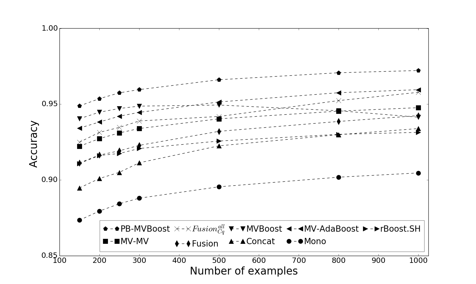
(a) MNIST1
(b) MNIST2
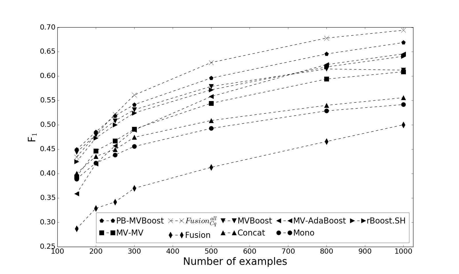
(c) Reuters

Figure 2: Evolution of accuracy and $F_{1}$-measure with respect to the number of labeled examples in the initial labeled training sets on MNIST₁, MNIST₂ and Reuters datasets.

5.2 Experimental Protocol

While the datasets are multiclass, we transformed them as binary tasks by considering one-vs-all classification problems: for each class we learn a binary classifier by considering all the learning samples from that class as positive examples and the others as negative examples. We consider different sizes of learning sample $S$ ($150$, $200$, $250$, $300$, $500$, $800$, $1000$) that are chosen randomly from the training data. Moreover, all the results are averaged over $20$ random runs of the experiments. Since the classes are unbalanced, we report the accuracy along with F1-measure for the methods and all the scores are averaged over all the one-vs-all classification problems.

We consider two multiview learning algorithms based on our two-step hierarchical strategy, and compare the PB-MVBoost algorithm described in Section 4, with a previously developed multiview learning algorithm Goyal et al. [2017], based on classifier late fusion approach Snoek et al. [2005], and referred to as Fusion${}_{\mathtt{Cq}}^{\mathtt{all}}$. Concretely, at the first level, this algorithm trains different view-specific linear SVM models with different hyperparameter $C$ values ($12$ values between $10^{-8}$ and $10^{3}$). And, at the second level, it learns a weighted combination over the predictions of view-specific voters using PAC-Bayesian algorithm CqBoostRoy et al. [2016] with a RBF kernel. Note that, algorithm CqBoost tends to minimize the PAC-Bayesian C-Bound Germain et al. [2015] controlling the trade-off between accuracy and disagreement among voters. The hyperparameter $\gamma$ of the RBF kernel is chosen over a set of $9$ values between $10^{-6}$ and $10^{2}$; and hyperparameter $\mu$ is chosen over a set of $8$ values between $10^{-8}$ and $10^{-1}$. To study the potential of our algorithms (Fusion${}_{\mathtt{Cq}}^{\mathtt{all}}$ and PB-MVBoost), we considered following $7$ baseline approaches:

• Mono: We learn a view-specific model for each view using a decision tree classifier and report the results of the best performing view.

• Concat: We learn one model using a decision tree classifier by concatenating features of all the views.

• Fusion${}_{\mathtt{dt}}^{\mathtt{}}$: This is a late fusion approach where we first learn the view-specific classifiers using $60\%$ of learning sample. Then, we learn a final multiview weighted model over the predictions of the view-specific classifiers. For this approach, we used decision tree classifiers at both levels of learning.

• MV-MV: We compute a multiview uniform majority vote (similar to approach followed by Amini et al. [2009]) over all the view-specific classifiers’ outputs in order to make final prediction. We learn view-specific classifiers using decision tree classifiers.

• rBoost.SH: This is the multiview learning algorithm proposed by Peng et al. [2011, 2017] where a single global distribution is maintained over the learning sample for all the views and the distribution over views are updated using multiarmed bandit framework. At each iteration, rBoost.SH selects a view according to the current distribution and learns the corresponding view-specific voter. For tuning the parameters, we followed the same experimental setting as Peng et al. [2017].

• MV-AdaBoost: This is a majority vote classifier over the view-specific voters trained using Adaboost algorithm. Here, our objective is to see the effect of maintaining separate distributions for all the views.

• MVBoost: This is a variant of our algorithm PB-MVBoost but without learning weights over views by optimizing multiview C-Bound. Here, our objective is to see the effect of learning weights over views on multiview learning.

For all boosting based approaches (rBoost.SH, MV-AdaBoost, MVBoost and PB-MVBoost), we learn the view-specific voters using a decision tree classifier with depth $2$ and $4$ as a weak classifier for MNIST, and Reuters RCV1/RCV2 datasets respectively. For all these approaches, we kept number of iterations $T=100$. For optimization of multiview C-Bound, we used Sequential Least SQuares Programming (SLSQP) implementation provided by SciPy Jones et al. [2001–] and the decision trees implementation from scikit-learn Pedregosa et al. [2011].

5.3 Results

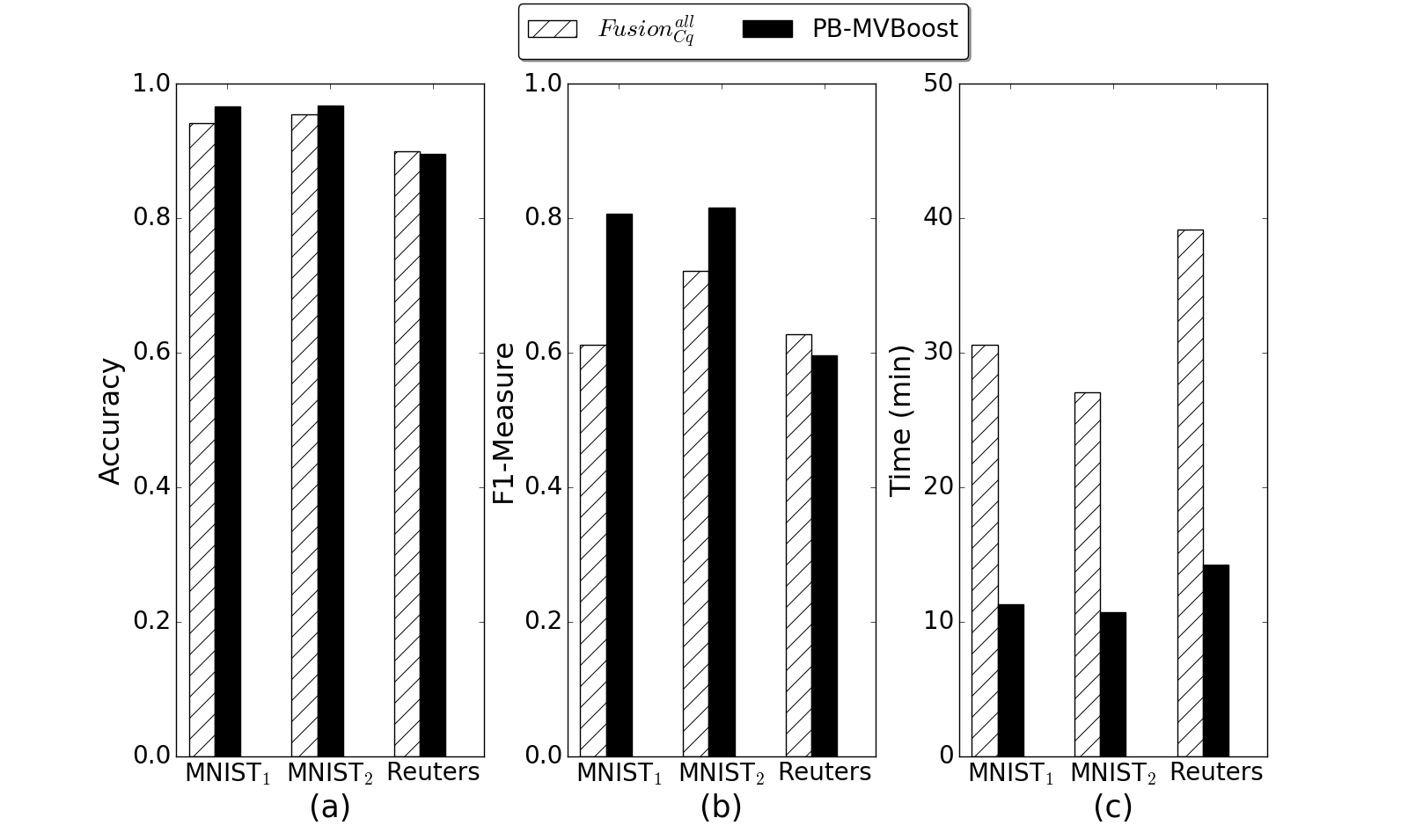
Figure 3: Comparison between Fusion${}_{\mathtt{Cq}}^{\mathtt{all}}$ and PB-MVBoost in terms Accuracy (a), F1-Measure (b) and Time Complexity (c) for $n=500$

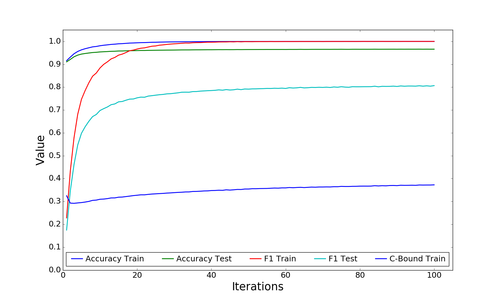
(a) MNIST₁

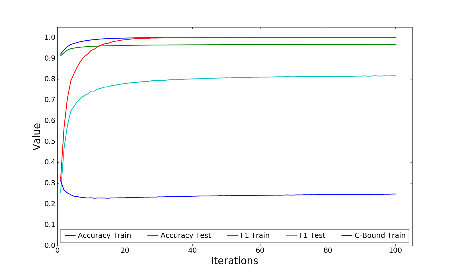
(b) MNIST₂

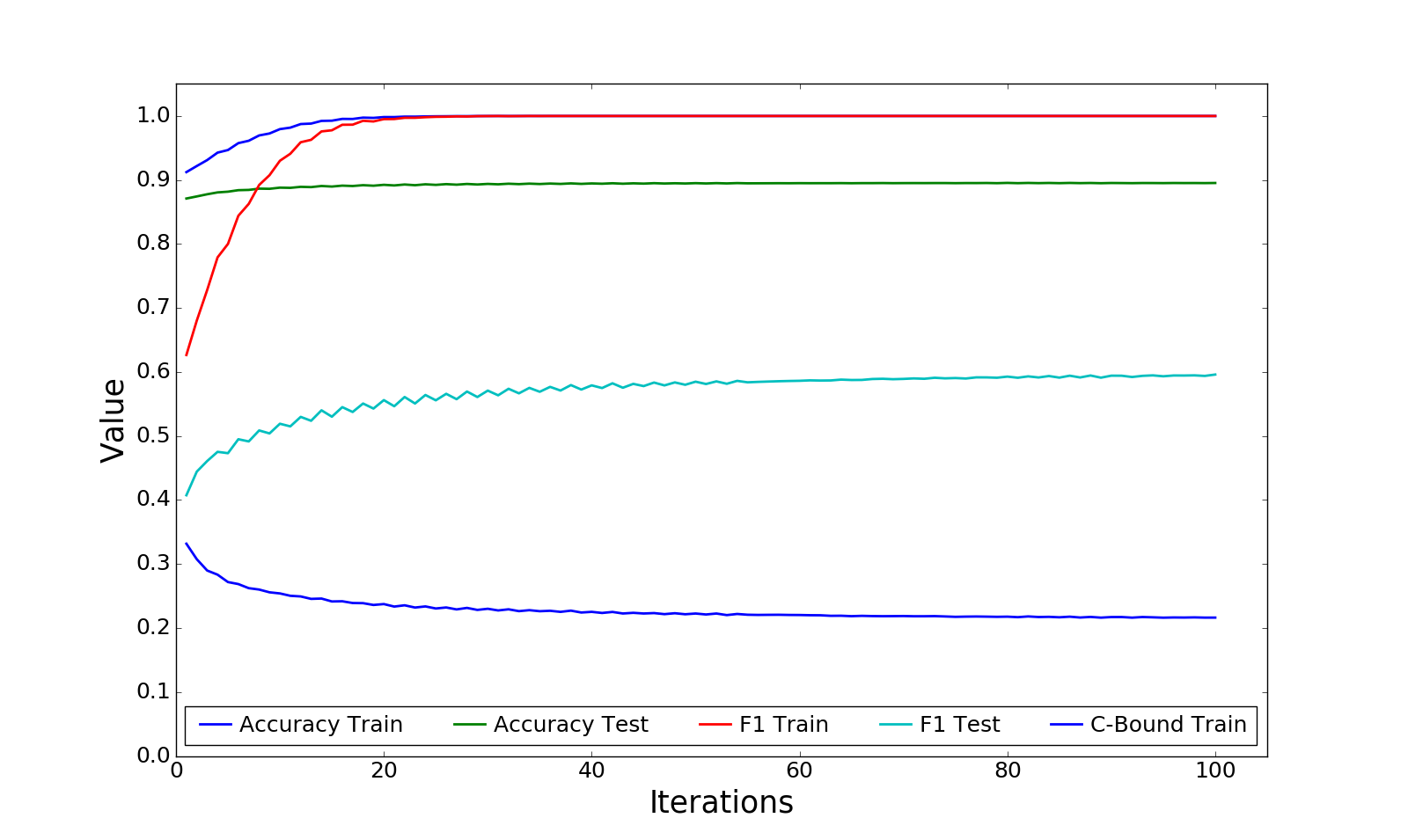
(c) Reuters

Figure 4: Plots for classification error and F1-measure on training and test data; and empirical multiview C-Bound on training data over the iterations for all datasets with $n=500$.

Firstly, we report the comparison of our algorithms Fusion${}_{\mathtt{Cq}}^{\mathtt{all}}$ and PB-MVBoost (for $m=500$) with all the considered baseline methods in Table 1. Secondly, Figure 2, illustrates the evolution of the performances according to the size of the learning sample. From the table, proposed two-step learning algorithm Fusion${}_{\mathtt{Cq}}^{\mathtt{all}}$ is significantly better than the baseline approaches for Reuters dataset. Whereas, our boosting based algorithm PB-MVBoost is significantly better than all the baseline approaches for all the datasets. This shows that considering a two-level hierarchical strategy in a PAC-Bayesian manner is an effective way to handle multiview learning.

In Figure 3, we compare proposed algorithms Fusion${}_{\mathtt{Cq}}^{\mathtt{all}}$ and PB-MVBoost in terms of accuracy, $F_{1}$-score and time complexity for $m=500$ examples. For MNIST datasets, PB-MVBoost is significantly better than Fusion${}_{\mathtt{Cq}}^{\mathtt{all}}$. For Reuters dataset, Fusion${}_{\mathtt{Cq}}^{\mathtt{all}}$ performs better than PB-MVBoost but computation time for Fusion${}_{\mathtt{Cq}}^{\mathtt{all}}$ is much higher than that of PB-MVBoost. Moreover, in Figure 2, we can see that the performance (in terms of $F_{1}$-score) for Fusion${}_{\mathtt{Cq}}^{\mathtt{all}}$ is worse than PB-MVBoost when we have less training examples ($n=150\mbox{ and }200$). This shows the proposed boosting based one-step algorithm PB-MVBoost is more stable and more effective for multiview learning.

From Table 1 and Figure 2, we can observe that MV-AdaBoost (where we have different distributions for each view over the learning sample) provides better results compared to other baselines in terms of accuracy but not in terms of F1-measure. On the other hand, MVBoost (where we have single global distribution over the learning sample but without learning weights over views) is better compared to other baselines in terms of F1-measure. Moreover, the performances of MVBoost first increases with an increase of the quantity of the training examples, then decreases. Whereas our algorithm PB-MVBoost provides the best results in terms of both accuracy and F1-measure, and leads to a monotonically increase of the performances with respect to the addition of labeled examples. This confirms that by maintaining a single global distribution over the views and learning the weights over the views using a PAC-Bayesian framework, we are able to take advantage of different representations (or views) of the data.

Finally, we plot behaviour of our algorithm PB-MVBoost over $T=100$ iterations on Figure 4 for all the datasets. We plot accuracy and F1-measure of learned models on training and test data along with empirical multiview C-Bound on training data at each iteration of our algorithm. Over the iterations, the F1-measure on the test data keeps on increasing for all the datasets even if F1-measure and accuracy on the training data reach the maximal value. This confirms that our algorithm handles unbalanced data well. Moreover, the empirical multiview C-Bound (which controls the trade-off between accuracy and diversity between views) keeps on decreasing over the iterations. This validates that by combining the PAC-Bayesian framework with the boosting one, we can empirically ensure the view specific information and diversity between the views for multiview learning.

6 Conclusion

In this paper, we provide a PAC-Bayesian analysis for a two-level hierarchical multiview learning approach with more than two views, when the model takes the form of a weighted majority vote over a set of functions/voters. We consider a hierarchy of weights modelized by distributions where for each view we aim at learning i) posterior $Q_{v}$ distributions over the view-specific voters capturing the view-specific information and ii) hyper-posterior $\rho_{v}$ distributions over the set of the views. Based on this strategy, we derived a general multiview PAC-Bayesian theorem that can be specialized to any convex function to compare the empirical and true risks of the stochastic multiview Gibbs classifier. We propose a boosting-based learning algorithm, called as PB-MVBoost. At each iteration of the algorithm, we learn the weights over the view-specific voters and the weights over the views by optimizing an upper-bound over the risk of the majority vote (the multiview C-Bound) that has the advantage to allow to control a trade-off between accuracy and the diversity between the views. The empirical evaluation shows that PB-MVBoost leads to good performances and confirms that our two-level PAC-Bayesian strategy is indeed a nice way to tackle multiview learning. Moreover, we compare the effect of maintaining separate distributions over the learning sample for each view; single global distribution over views; and single global distribution along with learning weights over views on results of multiview learning. We show that by maintaining a single global distribution over the learning sample for all the views and learning the weights over the views is an effective way to deal with multiview learning. In this way, we are able to capture the view-specific information and control the diversity between the views. Finally, we compare PB-MVBoost with a two-step learning algorithm Fusion${}_{\mathtt{Cq}}^{\mathtt{all}}$ which is based on PAC-Bayesian theory. We show that PB-MVBoost is more stable and computationally faster than Fusion${}_{\mathtt{Cq}}^{\mathtt{all}}$.

For future work, we would like to specialize our PAC-Bayesian generalization bounds to linear classifiers Germain et al. [2009] which will clearly open the door to derive theoretically founded multiview learning algorithms. We would also like to extend our algorithm to semi-supervised multiview learning where one has access to an additional unlabeled data during training. One possible way is to learn a view-specific voter using pseudo-labels (for unlabeled data) generated from the voters trained from other views (as done for example in Xu et al. [2016]). Another possible direction is to make use of unlabeled data while computing view-specific disagreement for optimizing multiview C-Bound. This clearly opens the door to derive theoretically founded algorithms for semi-supervised multiview learning using PAC-Bayesian theory. We would like to extend our algorithm to transfer learning setting where training and test data are drawn from different distributions. An interesting direction would be to bind the data distribution to the different views of the data, as in some recent zero-shot learning approaches Socher et al. [2013]. Moreover, we would like to extend our work to the case of missing views or incomplete views e.g. Amini et al. [2009] and Xu et al. [2015]. One possible solution is to learn the view-specific voters using available view-specific training examples and adapt the distribution over the learning sample accordingly.

Appendix

Appendix A Mathematical Tools

Theorem 3 (Markov’s ineq.)

For any random variable $X$ s.t. $\mathbb{E}(|X|)\!=\!\mu$, for any $a\!>\!0$, we have $\displaystyle\mathbb{P}(|X|\geq a)\leq\frac{\mu}{a}.$

Theorem 4 (Jensen’s ineq.)

For any random variable $X$, for any concave function $g$, we have $\displaystyle g(\operatorname*{\mathbb{E}}[X])\ \geq\ \operatorname*{\mathbb{E}}[g(X)].$

Theorem 5 (Cantelli-Chebyshev ineq.)

For any random variable $X$ s.t. $\mathbb{E}(X)\!=\!\mu$ and $\mathbf{Var}(X)=\sigma^{2}$, and for any $a\!>\!0$, we have $\mathbb{P}(X-\mu\geq a)\leq\frac{\sigma^{2}}{\sigma^{2}+a^{2}}.$

Appendix B Proof of $\mathcal{C}$-Bound for Multiview Learning (Lemma 1)

In this section, we present the proof of Lemma 1, inspired by the proof provided by Germain et al. [2015]. Firstly, we need to define the margin of the multiview weighted majority vote $B_{\rho}$ and its first and second statistical moments.

Definition 1

Let $M_{\rho}$ is a random variable that outputs the margin of the multiview weighted majority vote on the example $({\bf x},y)$ drawn from distribution $\mathcal{D}$, given by:

$$M_{\rho}({\bf x},y)={\displaystyle\operatorname*{\mathbb{E}}_{v\sim\rho}}\ {\displaystyle\operatorname*{\mathbb{E}}_{h\sim Q_{v}}}y\,h(x^{v}).$$

The first and second statistical moments of the margin are respectively given by

$$\mu_{1}(M_{\rho}^{\mathcal{D}})=\underset{({\bf x},y)\sim\mathcal{D}}{\mathbf{E}}M_{\rho}({\bf x},y).$$ (11)

and,

$$\mu_{2}(M_{\rho}^{\mathcal{D}}) =\underset{({\bf x},y)\sim\mathcal{D}}{\mathbf{E}}\big{[}M_{\rho}({\bf x},y)\big{]}^{2}$$

$$={\displaystyle\operatorname*{\mathbb{E}}_{{\bf x}\sim\mathcal{D}_{X}}}\ y^{2}\,\Big{[}{\displaystyle\operatorname*{\mathbb{E}}_{v\sim\rho}}\ {\displaystyle\operatorname*{\mathbb{E}}_{h\sim Q_{v}}}h(x^{v})\Big{]}^{2}={\displaystyle\operatorname*{\mathbb{E}}_{{\bf x}\sim\mathcal{D}_{X}}}\Big{[}{\displaystyle\operatorname*{\mathbb{E}}_{v\sim\rho}}\ {\displaystyle\operatorname*{\mathbb{E}}_{h\sim Q_{v}}}h(x^{v})\Big{]}^{2}.$$ (12)

According to this definition, the risk of the multiview weighted majority vote can be rewritten as follows:

$$R_{\mathcal{D}}(B_{\rho})=\underset{({\bf x},y)\sim\mathcal{D}}{\mathbb{P}}\big{(}M_{\rho}({\bf x},y)\leq 0\big{)}.$$

Moreover, the risk of the multiview Gibbs classifier can be expressed thanks to the first statistical moment of the margin. Note that in the binary setting where $y\in\{-1,1\}$ and $h:{\cal X}\to\{-1,1\}$, we have $\mathds{1}_{[h(x^{v})\neq y]}=\frac{1}{2}(1-y\,h(x^{v}))$, and therefore

$$R_{\mathcal{D}}(G_{\rho}) ={\displaystyle\operatorname*{\mathbb{E}}_{(\mathbf{x},y)\sim\mathcal{D}}}\ {\displaystyle\operatorname*{\mathbb{E}}_{v\sim\rho}}\ {\displaystyle\operatorname*{\mathbb{E}}_{h\sim Q_{v}}}\mathds{1}_{[h(x^{v})\neq y]}$$

$$=\frac{1}{2}\bigg{(}1-{\displaystyle\operatorname*{\mathbb{E}}_{({\bf x},y)\sim\mathcal{D}}}\ {\displaystyle\operatorname*{\mathbb{E}}_{v\sim\rho}}\ {\displaystyle\operatorname*{\mathbb{E}}_{h\sim Q_{v}}}y\,h(x^{v})\bigg{)}$$ (13)

$$=\frac{1}{2}(1-\mu_{1}(M_{\rho}^{\mathcal{D}}))\,.$$

Similarly, the expected disagreement can be expressed thanks to the second statistical moment of the margin by

$$d_{{\cal D}}(\rho) =\operatorname*{\mathbb{E}}_{{\bf x}\sim\mathcal{D}_{\mathcal{X}}}\operatorname*{\mathbb{E}}_{v\sim\rho}\operatorname*{\mathbb{E}}_{v^{\prime}\sim\rho}\operatorname*{\mathbb{E}}_{h\sim Q_{v}}\operatorname*{\mathbb{E}}_{h^{\prime}\sim Q_{v^{\prime}}}\mathds{1}_{[h(x^{v}){\neq}h^{\prime}(x^{v^{\prime}})]}$$

$$=\frac{1}{2}\bigg{(}1-\operatorname*{\mathbb{E}}_{{\bf x}\sim\mathcal{D}_{\mathcal{X}}}\operatorname*{\mathbb{E}}_{v\sim\rho}\operatorname*{\mathbb{E}}_{v^{\prime}\sim\rho}\operatorname*{\mathbb{E}}_{h\sim Q_{v}}\operatorname*{\mathbb{E}}_{h\sim Q_{v^{\prime}}}h(x^{v})\times h^{\prime}(x^{v^{\prime}})\bigg{)}$$

$$=\frac{1}{2}\bigg{(}1-\operatorname*{\mathbb{E}}_{{\bf x}\sim\mathcal{D}_{\mathcal{X}}}\Big{[}\operatorname*{\mathbb{E}}_{v\sim\rho}\operatorname*{\mathbb{E}}_{h\sim Q_{v}}h(x^{v})\Big{]}\times\Big{[}\operatorname*{\mathbb{E}}_{v^{\prime}\sim\rho}\operatorname*{\mathbb{E}}_{h^{\prime}\sim Q_{v^{\prime}}}h^{\prime}(x^{v^{\prime}})\Big{]}\bigg{)}$$

$$=\frac{1}{2}\bigg{(}1-{\displaystyle\operatorname*{\mathbb{E}}_{{\bf x}\sim\mathcal{D}_{\mathcal{X}}}}\bigg{[}{\displaystyle\operatorname*{\mathbb{E}}_{v\sim\rho}}\,{\displaystyle\operatorname*{\mathbb{E}}_{h\sim Q_{v}}}h(x^{v})\bigg{]}^{2}\bigg{)}$$ (14)

$$=\frac{1}{2}(1-\mu_{2}(M_{\rho}^{\mathcal{D}}))\,.$$

From above, we can easily deduce that $0\leq d_{{\cal D}}(\rho)\leq 1/2$ as $0\leq\mu_{2}(M_{\rho}^{\mathcal{D}})\leq 1$. Therefore, the variance of the margin can be written as:

$$\begin{split}\text{Var}(M_{\rho}^{\mathcal{D}})&=\underset{({\bf x},y)\sim\mathcal{D}}{\textbf{Var}}(M_{\rho}({\bf x},y))\\ &=\mu_{2}(M_{\rho}^{\mathcal{D}})-(\mu_{1}(M_{\rho}^{\mathcal{D}}))^{2}.\end{split}$$ (15)

The proof of the $\mathcal{C}$-bound

Proof.  By making use of one-sided Chebyshev inequality (Theorem 5 of A), with $X=-M_{\rho}({\bf x},y)$, $\mu={\displaystyle\operatorname*{\mathbb{E}}_{({\bf x},y)\sim\mathcal{D}}}(M_{\rho}({\bf x},y))$ and $a={\displaystyle\operatorname*{\mathbb{E}}_{({\bf x},y)\sim\mathcal{D}}}M_{\rho}({\bf x},y)$, we have

$$R_{\mathcal{D}}(B_{\rho}) =\underset{({\bf x},y)\sim\mathcal{D}}{\mathbb{P}}\big{(}M_{\rho}({\bf x},y)\leq 0\big{)}$$

$$=\underset{({\bf x},y)\sim\mathcal{D}}{\mathbb{P}}\bigg{(}-M_{\rho}({\bf x},y)+{\displaystyle\operatorname*{\mathbb{E}}_{({\bf x},y)\sim\mathcal{D}}}M_{\rho}({\bf x},y)\geq{\displaystyle\operatorname*{\mathbb{E}}_{({\bf x},y)\sim\mathcal{D}}}M_{\rho}({\bf x},y)\bigg{)}$$

$$\leq\frac{\underset{({\bf x},y)\sim\mathcal{D}}{\textbf{Var}}(M_{\rho}({\bf x},y))}{\underset{({\bf x},y)\sim\mathcal{D}}{\textbf{Var}}(M_{\rho}({\bf x},y))+\bigg{(}{\displaystyle\operatorname*{\mathbb{E}}_{({\bf x},y)\sim\mathcal{D}}}M_{\rho}({\bf x},y)\bigg{)}^{2}}$$

$$=\frac{\text{Var}(M_{\rho}^{\mathcal{D}})}{\mu_{2}(M_{\rho}^{\mathcal{D}})-\bigg{(}\mu_{1}(M_{\rho}^{\mathcal{D}})\bigg{)}^{2}+\bigg{(}\mu_{1}(M_{\rho}^{\mathcal{D}})\bigg{)}^{2}}$$

$$=\frac{\text{Var}(M_{\rho}^{\mathcal{D}})}{\mu_{2}(M_{\rho}^{\mathcal{D}})}$$

$$=\frac{\mu_{2}(M_{\rho}^{\mathcal{D}})-\bigg{(}\mu_{1}(M_{\rho}^{\mathcal{D}})\bigg{)}^{2}}{\mu_{2}(M_{\rho}^{\mathcal{D}})}$$

$$=1-\frac{\bigg{(}\mu_{1}(M_{\rho}^{\mathcal{D}})\bigg{)}^{2}}{\mu_{2}(M_{\rho}^{\mathcal{D}})}$$

$$=1-\frac{\bigg{(}1-2\,R_{\mathcal{D}}(G_{\rho})\bigg{)}^{2}}{1-2\,d_{{\cal D}}(\rho)}$$

 

Appendix C Proof of Lemma 2

We have

$${\displaystyle\operatorname*{\mathbb{E}}_{v\sim\rho}}\,{\displaystyle\operatorname*{\mathbb{E}}_{h\sim Q_{v}}}\phi(h)\ =\ {\displaystyle\operatorname*{\mathbb{E}}_{v\sim\rho}}\ {\displaystyle\operatorname*{\mathbb{E}}_{h\sim Q_{v}}}\ln e^{\phi(h)}$$

$$=\ {\displaystyle\operatorname*{\mathbb{E}}_{v\sim\rho}}\ {\displaystyle\operatorname*{\mathbb{E}}_{h\sim Q_{v}}}\ln\bigg{(}\frac{Q_{v}(h)}{P_{v}(h)}\frac{P_{v}(h)}{Q_{v}(h)}e^{\phi(h)}\bigg{)}$$

$$=\ {\displaystyle\operatorname*{\mathbb{E}}_{v\sim\rho}}\ \bigg{[}{\displaystyle\operatorname*{\mathbb{E}}_{h\sim Q_{v}}}\ln\bigg{(}\frac{Q_{v}(h)}{P_{v}(h)}\bigg{)}+{\displaystyle\operatorname*{\mathbb{E}}_{h\sim Q_{v}}}\ln\bigg{(}\frac{P_{v}(h)}{Q_{v}(h)}e^{\phi(h)}\bigg{)}\bigg{]}.$$

According to the Kullback-Leibler definition, we have

$${\displaystyle\operatorname*{\mathbb{E}}_{v\sim\rho}}\,{\displaystyle\operatorname*{\mathbb{E}}_{h\sim Q_{v}}}\phi(h)\ =\ {\displaystyle\operatorname*{\mathbb{E}}_{v\sim\rho}}\bigg{[}\operatorname{KL}(Q_{v}\|P_{v})+{\displaystyle\operatorname*{\mathbb{E}}_{h\sim Q_{v}}}\ln\bigg{(}\frac{P_{v}(h)}{Q_{v}(h)}e^{\phi(h)}\bigg{)}\bigg{]}.$$

By applying Jensen’s inequality (Theorem 4, in Appendix) on the concave function $\ln$, we have

$${\displaystyle\operatorname*{\mathbb{E}}_{v\sim\rho}}\,{\displaystyle\operatorname*{\mathbb{E}}_{h\sim Q_{v}}}\phi(h)\ \leq\ {\displaystyle\operatorname*{\mathbb{E}}_{v\sim\rho}}\ \bigg{[}\operatorname{KL}(Q_{v}\|P_{v})+\ln\bigg{(}{\displaystyle\operatorname*{\mathbb{E}}_{h\sim P_{v}}}e^{\phi(h)}\bigg{)}\bigg{]}$$

$$=\ {\displaystyle\operatorname*{\mathbb{E}}_{v\sim\rho}}\operatorname{KL}(Q_{v}\|P_{v})+{\displaystyle\operatorname*{\mathbb{E}}_{v\sim\rho}}\ln\bigg{(}\frac{\rho(v)}{\pi(v)}\frac{\pi(v)}{\rho(v)}{\displaystyle\operatorname*{\mathbb{E}}_{h\sim P_{v}}}e^{\phi(h)}\bigg{)}$$

$$=\ {\displaystyle\operatorname*{\mathbb{E}}_{v\sim\rho}}\operatorname{KL}(Q_{v}\|P_{v})+\operatorname{KL}(\rho\|\pi)+{\displaystyle\operatorname*{\mathbb{E}}_{v\sim\rho}}\ln\bigg{(}\frac{\pi(v)}{\rho(v)}{\displaystyle\operatorname*{\mathbb{E}}_{h\sim P_{v}}}e^{\phi(h)}\bigg{)}.$$

Finally, we apply again the Jensen inequality (Theorem 4) on $\ln$ to obtain the lemma.

Appendix D A Catoni-Like Theorem—Proof of Corollary 1

The result comes from Theorem 1 by taking $D(a,b)\!=\!\mathcal{F}(b)\!-\!Ca$, for a convex $\cal F$ and $C\!>\!0$, and by upper-bounding ${\displaystyle\operatorname*{\mathbb{E}}_{S\sim({\cal D})^{n}}}{\displaystyle\operatorname*{\mathbb{E}}_{v\sim\pi}}{\displaystyle\operatorname*{\mathbb{E}}_{h\sim P_{v}}}e^{nD(R_{S}(h),R_{\cal D}(h))}$. We consider $R_{S}(h)$ as a random variable following a binomial distribution of $n$ trials with a probability of success $R(h)$. We have:

$${\displaystyle\operatorname*{\mathbb{E}}_{S\sim({\cal D})^{n}}}\,{\displaystyle\operatorname*{\mathbb{E}}_{v\sim\pi}}\,{\displaystyle\operatorname*{\mathbb{E}}_{h\sim P_{v}}}e^{n\,D(R_{S}(h),R_{\cal D}(h))}$$

$$=\!{\displaystyle\operatorname*{\mathbb{E}}_{S\sim({\cal D})^{n}}}\,{\displaystyle\operatorname*{\mathbb{E}}_{v\sim\pi}}\,{\displaystyle\operatorname*{\mathbb{E}}_{h\sim P_{v}}}e^{n\,\mathcal{F}(R_{\cal D}(h)-C\,n\,R_{S}(h))}$$

$${\small=\!\!{\displaystyle\operatorname*{\mathbb{E}}_{S\sim({\cal D})^{n}}}{\displaystyle\operatorname*{\mathbb{E}}_{v\sim\pi}}{\displaystyle\operatorname*{\mathbb{E}}_{h\sim P_{v}}}\!\!\!e^{n\,\mathcal{F}(R_{\cal D}(h))}\sum_{k=0}^{n}\underset{S\sim({\cal D})^{n}}{\Pr}\!\!\left(\!R_{S}(h)\!=\!\frac{k}{n}\!\right)\!e^{\!-Ck}}$$

$${\small=\!\!\!\!\!{\displaystyle\operatorname*{\mathbb{E}}_{S\sim({\cal D})^{\!n}}}{\displaystyle\operatorname*{\mathbb{E}}_{v\sim\pi}}\,{\displaystyle\operatorname*{\mathbb{E}}_{h\sim P_{v}}}\!\!\!e^{n\mathcal{F}\!(R_{\cal D}(h))\!}\sum_{k=0}^{n}\!{\textstyle\binom{n}{k}}R_{\cal D}(h)^{k}(1\!-\!R_{\cal D}(h))^{n\!-\!k\!}e^{-Ck}}$$

$${\small=\!\!{\displaystyle\operatorname*{\mathbb{E}}_{S\sim({\cal D})^{n}}}\,{\displaystyle\operatorname*{\mathbb{E}}_{v\sim\pi}}\,{\displaystyle\operatorname*{\mathbb{E}}_{h\sim P_{v}}}\!e^{n\mathcal{F}(R_{\cal D}(h))}\big{(}R_{\cal D}(h)\,e^{-\!\,C}\!\!+\!(1\!-\!R_{\cal D}(h))\big{)}^{n}\!\!.}$$

The corollary is obtained with $\mathcal{F}(p)\!=\!\ln\frac{1}{(1\!-\!p[1\!-\!e^{-C}])}$.

References

• Alquier et al. [2015] Pierre Alquier, James Ridgway, and Nicolas Chopin. On the properties of variational approximations of Gibbs posteriors. ArXiv e-prints, 2015. URL http://arxiv.org/abs/1506.04091.
• Amini et al. [2009] Massih-Reza Amini, Nicolas Usunier, and Cyril Goutte. Learning from Multiple Partially Observed Views - an Application to Multilingual Text Categorization. In NIPS, pages 28–36, 2009.
• Atrey et al. [2010] Pradeep K. Atrey, M. Anwar Hossain, Abdulmotaleb El-Saddik, and Mohan S. Kankanhalli. Multimodal fusion for multimedia analysis: a survey. Multimedia Syst., 16(6):345–379, 2010.
• Blum and Mitchell [1998] Avrim Blum and Tom M. Mitchell. Combining Labeled and Unlabeled Data with Co-Training. In COLT, pages 92–100, 1998.
• Brown and Kuncheva [2010] Gavin Brown and Ludmila I. Kuncheva. “good” and “bad” diversity in majority vote ensembles. In Neamat El Gayar, Josef Kittler, and Fabio Roli, editors, Multiple Classifier Systems, pages 124–133, Berlin, Heidelberg, 2010. Springer Berlin Heidelberg. ISBN 978-3-642-12127-2.
• Catoni [2007] Olivier Catoni. PAC-Bayesian supervised classification: the thermodynamics of statistical learning, volume 56. Inst. of Mathematical Statistic, 2007.
• Chapelle et al. [2010] Olivier Chapelle, Bernhard Schlkopf, and Alexander Zien. Semi-Supervised Learning. The MIT Press, 1st edition, 2010. ISBN 0262514125, 9780262514125.
• Chen and Denoyer [2017] Mickaël Chen and Ludovic Denoyer. Multi-view generative adversarial networks. In Machine Learning and Knowledge Discovery in Databases - European Conference, ECML PKDD 2017, Skopje, Macedonia, September 18-22, 2017, Proceedings, Part II, pages 175–188, 2017. doi: 10.1007/978-3-319-71246-8˙11. URL https://doi.org/10.1007/978-3-319-71246-8_11.
• Dietterich [2000] Thomas G. Dietterich. Ensemble methods in machine learning. In Multiple Classifier Systems, pages 1–15, 2000.
• Donsker and Varadhan [1975] Monroe D Donsker and SR Srinivasa Varadhan. Asymptotic evaluation of certain markov process expectations for large time, i. Communications on Pure and Applied Mathematics, 28(1):1–47, 1975.
• D ez-Pastor et al. [2015] Jos  F. D ez-Pastor, Juan J. Rodr guez, C sar I. Garc a-Osorio, and Ludmila I. Kuncheva. Diversity techniques improve the performance of the best imbalance learning ensembles. Information Sciences, 325:98 – 117, 2015. ISSN 0020-0255. doi: https://doi.org/10.1016/j.ins.2015.07.025. URL http://www.sciencedirect.com/science/article/pii/S0020025515005186.
• Freund [1995] Yoav Freund. Boosting a weak learning algorithm by majority. Inf. Comput., 121(2):256–285, September 1995. ISSN 0890-5401. doi: 10.1006/inco.1995.1136. URL http://dx.doi.org/10.1006/inco.1995.1136.
• Freund and Schapire [1997] Yoav Freund and Robert E Schapire. A decision-theoretic generalization of on-line learning and an application to boosting. J. Comput. Syst. Sci., 55(1):119–139, August 1997. ISSN 0022-0000. doi: 10.1006/jcss.1997.1504. URL http://dx.doi.org/10.1006/jcss.1997.1504.
• Germain et al. [2009] Pascal Germain, Alexandre Lacasse, François Laviolette, and Mario Marchand. PAC-Bayesian learning of linear classifiers. In ICML, pages 353–360, 2009.
• Germain et al. [2015] Pascal Germain, Alexandre Lacasse, François Laviolette, Mario Marchand, and Jean-Francis Roy. Risk bounds for the majority vote: from a PAC-Bayesian analysis to a learning algorithm. JMLR, 16:787–860, 2015.
• Germain et al. [2016] Pascal Germain, Amaury Habrard, François Laviolette, and Emilie Morvant. A new PAC-Bayesian perspective on domain adaptation. In Proceedings of the 33nd International Conference on Machine Learning, ICML 2016, New York City, NY, USA, June 19-24, 2016, pages 859–868, 2016. URL http://jmlr.org/proceedings/papers/v48/germain16.html.
• Goyal et al. [2017] Anil Goyal, Emilie Morvant, Pascal Germain, and Massih-Reza Amini. PAC-Bayesian Analysis for a Two-Step Hierarchical Multiview Learning Approach. In Machine Learning and Knowledge Discovery in Databases - European Conference, ECML PKDD 2017, Skopje, Macedonia, September 18-22, 2017, Proceedings, Part II, pages 205–221, 2017. doi: 10.1007/978-3-319-71246-8˙13. URL https://doi.org/10.1007/978-3-319-71246-8_13.
• Janodet et al. [2009] Jean-Christophe Janodet, Marc Sebban, and Henri-Maxime Suchier. Boosting Classifiers built from Different Subsets of Features. Fundamenta Informaticae, 94(2009):1–21, July 2009. doi: 10.3233/FI-2009-131. URL https://hal.archives-ouvertes.fr/hal-00403242.
• Jones et al. [2001–] Eric Jones, Travis Oliphant, Pearu Peterson, et al. SciPy: Open source scientific tools for Python, 2001–. URL http://www.scipy.org/.
• Koço and Capponi [2011] Sokol Koço and Cécile Capponi. A boosting approach to multiview classification with cooperation. In Dimitrios Gunopulos, Thomas Hofmann, Donato Malerba, and Michalis Vazirgiannis, editors, Machine Learning and Knowledge Discovery in Databases, pages 209–228, Berlin, Heidelberg, 2011. Springer Berlin Heidelberg. ISBN 978-3-642-23783-6.
• Kuncheva [2004] Ludmila I. Kuncheva. Combining Pattern Classifiers: Methods and Algorithms. Wiley-Interscience, 2004. ISBN 0471210781.
• Lacasse et al. [2006] Alexandre Lacasse, Francois Laviolette, Mario Marchand, Pascal Germain, and Nicolas Usunier. PAC-Bayes bounds for the risk of the majority vote and the variance of the Gibbs classifier. In NIPS, pages 769–776, 2006.
• Langford [2005] John Langford. Tutorial on practical prediction theory for classification. JMLR, 6:273–306, 2005.
• Langford and Shawe-Taylor [2002] John Langford and John Shawe-Taylor. PAC-Bayes & margins. In NIPS, pages 423–430. MIT Press, 2002.
• Lecun et al. [1998] Yann Lecun, L on Bottou, Yoshua Bengio, and Patrick Haffner. Gradient-based learning applied to document recognition. In Proceedings of the IEEE, pages 2278–2324, 1998.
• Maillard and Vayatis [2009] Odalric-Ambrym Maillard and Nicolas Vayatis. Complexity versus agreement for many views. In ALT, pages 232–246, 2009.
• McAllester [1999] David A. McAllester. Some PAC-Bayesian theorems. Machine Learning, 37:355–363, 1999.
• McAllester [2003] David A. McAllester. PAC-Bayesian stochastic model selection. In Machine Learning, pages 5–21, 2003.
• Morvant et al. [2014] Emilie Morvant, Amaury Habrard, and Stéphane Ayache. Majority vote of diverse classifiers for late fusion. In Structural, Syntactic, and Statistical Pattern Recognition - Joint IAPR International Workshop, S+SSPR 2014, Joensuu, Finland, August 20-22, 2014. Proceedings, pages 153–162, 2014. doi: 10.1007/978-3-662-44415-3˙16. URL https://doi.org/10.1007/978-3-662-44415-3_16.
• Parrado-Hernández et al. [2012] Emilio Parrado-Hernández, Amiran Ambroladze, John Shawe-Taylor, and Shiliang Sun. PAC-bayes bounds with data dependent priors. JMLR, 13:3507–3531, 2012.
• Pedregosa et al. [2011] F. Pedregosa, G. Varoquaux, A. Gramfort, V. Michel, B. Thirion, O. Grisel, M. Blondel, P. Prettenhofer, R. Weiss, V. Dubourg, J. Vanderplas, A. Passos, D. Cournapeau, M. Brucher, M. Perrot, and E. Duchesnay. Scikit-learn: Machine learning in Python. Journal of Machine Learning Research, 12:2825–2830, 2011.
• Peng et al. [2017] J. Peng, A. J. Aved, G. Seetharaman, and K. Palaniappan. Multiview boosting with information propagation for classification. IEEE Transactions on Neural Networks and Learning Systems, PP(99):1–13, 2017. ISSN 2162-237X. doi: 10.1109/TNNLS.2016.2637881.
• Peng et al. [2011] Jing Peng, Costin Barbu, Guna Seetharaman, Wei Fan, Xian Wu, and Kannappan Palaniappan. Shareboost: Boosting for multi-view learning with performance guarantees. In Machine Learning and Knowledge Discovery in Databases - European Conference, ECML PKDD 2011, Athens, Greece, September 5-9, 2011, Proceedings, Part II, pages 597–612, 2011. doi: 10.1007/978-3-642-23783-6˙38. URL https://doi.org/10.1007/978-3-642-23783-6_38.
• Re and Valentini [2012] M. Re and G. Valentini. Ensemble methods: a review. Advances in machine learning and data mining for astronomy, pages 563–582, 2012.
• Roy et al. [2011] Jean-Francis Roy, François Laviolette, and Mario Marchand. From pac-bayes bounds to quadratic programs for majority votes. In Proceedings of the 28th International Conference on Machine Learning, ICML 2011, Bellevue, Washington, USA, June 28 - July 2, 2011, pages 649–656, 2011.
• Roy et al. [2016] Jean-Francis Roy, Mario Marchand, and François Laviolette. A column generation bound minimization approach with PAC-Bayesian generalization guarantees. In Proceedings of the 19th International Conference on Artificial Intelligence and Statistics, pages 1241–1249, 2016.
• Schapire [1999] Robert E. Schapire. A brief introduction to boosting. In Proceedings of the 16th International Joint Conference on Artificial Intelligence - Volume 2, IJCAI’99, pages 1401–1406, San Francisco, CA, USA, 1999. Morgan Kaufmann Publishers Inc. URL http://dl.acm.org/citation.cfm?id=1624312.1624417.
• Schapire [2003] Robert E. Schapire. The Boosting Approach to Machine Learning: An Overview. Springer New York, New York, NY, 2003. ISBN 978-0-387-21579-2. doi: 10.1007/978-0-387-21579-2˙9. URL https://doi.org/10.1007/978-0-387-21579-2_9.
• Seeger [2002] Matthias W. Seeger. PAC-Bayesian generalisation error bounds for gaussian process classification. JMLR, 3:233–269, 2002.
• Shawe-Taylor and Langford [2003] John Shawe-Taylor and John Langford. PAC-Bayes & margins. Advances in Neural Information Processing Systems, 15:439, 2003.
• Snoek et al. [2005] Cees Snoek, Marcel Worring, and Arnold W. M. Smeulders. Early versus late fusion in semantic video analysis. In ACM Multimedia, pages 399–402, 2005.
• Socher et al. [2013] Richard Socher, Milind Ganjoo, Christopher D Manning, and Andrew Ng. Zero-shot learning through cross-modal transfer. In Advances in Neural Information Processing Systems 26, pages 935–943, 2013.
• Sun [2013] Shiliang Sun. A survey of multi-view machine learning. Neural Comput Appl, 23(7-8):2031–2038, 2013.
• Sun et al. [2017] Shiliang Sun, John Shawe-Taylor, and Liang Mao. PAC-Bayes analysis of multi-view learning. Information Fusion, 35:117–131, 2017.
• Xiao and Guo [2012] Min Xiao and Yuhong Guo. Multi-view adaboost for multilingual subjectivity analysis. In COLING 2012, 24th International Conference on Computational Linguistics, Proceedings of the Conference: Technical Papers, 8-15 December 2012, Mumbai, India, pages 2851–2866, 2012. URL http://aclweb.org/anthology/C/C12/C12-1174.pdf.
• Xu et al. [2015] C. Xu, D. Tao, and C. Xu. Multi-view learning with incomplete views. IEEE Transactions on Image Processing, 24(12):5812–5825, 2015.
• Xu et al. [2016] X. Xu, W. Li, D. Xu, and I. W. Tsang. Co-labeling for multi-view weakly labeled learning. IEEE Transactions on Pattern Analysis and Machine Intelligence, 38(6):1113–1125, June 2016. ISSN 0162-8828.
• Xu and Sun [2010] Zhijie Xu and Shiliang Sun. An algorithm on multi-view adaboost. In Kok Wai Wong, B. Sumudu U. Mendis, and Abdesselam Bouzerdoum, editors, Neural Information Processing. Theory and Algorithms, pages 355–362, Berlin, Heidelberg, 2010. Springer Berlin Heidelberg. ISBN 978-3-642-17537-4.