The scattering of FRBs by the intergalactic medium: variations, strength and dependence on dispersion measures

Abstract

The scattering of fast radio bursts (FRBs) by the intergalactic medium (IGM) is explored using cosmological hydrodynamical simulations. We confirm that the scattering by the clumpy IGM has significant line-of-sight variations. We demonstrate that the scattering by the IGM in the voids and walls of the cosmic web is weak, but it can be significantly enhanced by the gas in clusters and filaments. The observed non-monotonic dependence of the FRB widths on the dispersion measures (DM) cannot determine whether the IGM is an important scattering matter or not. The IGM may dominate the scattering of some FRBs, and the host galaxy dominates others. For the former case, the scattering should be primarily caused by the medium in clusters. A mock sample of 500 sources shows that $\tau_{\rm{IGM}}\propto\rm{DM_{IGM}}^{1.6-2.1}$ at $z<1.5$. Assuming that the turbulence follows Kolmogorov scaling, we find that an outer scale of $L_{0}\sim 5\,$pc is required to make $\tau_{\rm{IGM}}\sim 1-10\,$ms at $\nu=1\,$ GHz. The required $L_{0}\sim 5\,$pc can alleviate the tension in the timescales of turbulent heating and cooling but is still $\sim 4$ orders of magnitude lower than the presumed injection scale of turbulence in the IGM. The gap is expected to be effectively shortened if the simulation resolution is further increased. The mechanisms that may further reduce the gap are shortly discussed. If future observations can justify the role of the IGM in the broadening of FRBs, it can help to probe the gas in clusters and filaments.

1 Introduction

Fast radio bursts (FRBs) are a recently discovered class of millisecond-duration radio transients (e.g., Lorimer et al. 2007; Thornton et al. 2013; Champion et al. 2016; Petroff et al. 2016). The dispersion measures (DMs) of observed FRBs range from 176 to a few thousands (the highest value until now is 2596 ${\rm{pc\,cm^{-3}}}$; see Bhandari et al. 2018). For most observed events, their DMs are much higher than the expected value because of the medium in the Milky Way, which indicates that FRBs are of extra-galactic origin. It is suggested that the DMs of FRBs are substantially contributed by the intergalactic medium (IGM), which can be used in principle to probe the properties of the IGM(Ioka 2003; Inoue 2004; Deng & Zhang 2014; McQuinn 2014).

The broadening of the pulse width because of scattering by the turbulent medium, i.e., $\tau$, is also an important parameter of FRBs. The scattering by the Galaxy is inadequate to explain the broadening of several FRBs at high latitudes. The location of the non-galactic scattering has not been determined because both the host galaxy medium and IGM may play important roles. The host can cause significant broadening that is sufficiently strong to explain the observation (Cordes et al. 2016; Katz 2016; Xu & Zhang 2016, hereafter XZ16). Meanwhile, the contribution of the IGM is under debate. Macquart & Koay (2013, hereafter MK13) estimated that the broadening contributed by the extended, diffuse IGM at $z<3$ was approximately $\tau_{\rm{IGM}}\lesssim 1\,$ms at $\nu\sim 300$ MHz. They showed that the intervening halo gas and intra-cluster medium (ICM) along the LOS might be capable of producing $\tau_{\rm{IGM}}\sim 5\,$ms at $\nu\sim 300$ MHz, but they doubted the probability. Two major concerns were recently raised against the IGM as an important scattering matter: (1) To produce $\tau_{\rm{IGM}}\sim 5\,$ms at $\nu\sim 300$ MHz, the outer scale of turbulence with the Kolmogorov spectrum must be $\sim 10^{-2}\,$pc, which appears too small compared to the often presumed injection scale ($\geq 100\,$kpc) and is incompatible with the cooling rate of the IGM(Luan & Goldreich 2014, XZ16). (2) The non-monotonic dependence of the observed FRB widths on DMs is inconsistent with the expectations for intergalactic scattering(Katz 2016).

However, Yao et al. (2017) argued that the broadening of observed FRBs tended to increase with the DM contributed by the IGM. In fact, the strength of this tendency may have been weakened by the large lines-of-sight(LOS) variations in the scatter measure (SM) caused by the clumpy IGM (MK13). The anisotropic gravitational collapse makes the initially small-amplitude density fluctuations of cosmic matter form a large scale spatial pattern known as the cosmic web, which consists of clusters, filaments, walls and voids (Zel’dovich 1970; Bond et al. 1996). The density perturbation growth in the late nonlinear stages because of gravitational instability can be described by a turbulence model (Shandarin & Zel’dovich 1989). In addition, the accretion of matter to collapsed objects is highly anisotropic and non-homogenous. The gas accreted into dark matter halos occurs in both hot and cold mode, and contains clumps of various size(Dekel et al. 2009). When low mass dark matter halos falling into the gaseous halo of more massive dark matter halos, both thermal and dynamical instabilities, such as the Kelvin-Helmholtz and Rayleigh-Taylor instability, will be triggered and can lead to density fluctuations on scale smaller than the satellite halos(e.g., Mayer et al. 2006; Abramson et al. 2011). Recent cosmological hydrodynamical simulations without a star formation process found considerable density fluctuations of gas on the resolution scale, i.e., tens of kpc, particularly in clusters and filaments(Vazza et al. 2010; Zhu & Feng 2017). Cosmological hydrodynamical simulations of galaxy formation have shown density and temperature fluctuation on their resolution scale of a few kpc in regions within and outside the dark matter halos (e.g., Vogelsberger et al. 2012, Nelson et al. 2013 ).

In this work, we probe the scattering of FRBs by the clumpy IGM using cosmological hydrodynamical simulations and revisit the required outer scales of turbulence that can make the IGM an important contributor to the broadening of FRBs. We present the numerical methodology in Section 2. The DM and SM contributed by the IGM residing in the cosmic web are probed in Section 3. We then probe the scattering of FRBs by the IGM in Section 4. In Section 5, we discuss the required outer scales of turbulence to make the IGM play important roles in the broadening of FRBS. Then we summarize our results in Section 6.

2 methodlogy

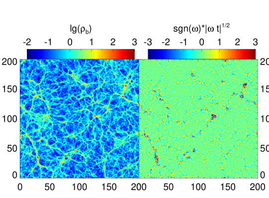
Figure 1: Density (left) and projected vorticity (right) of the IGM in a slice of thickness $0.39h^{-1}$ Mpc at $z=0$. The red/blue color in the right panel indicates that the vorticity is toward/away from the observer.

2.1 simulations

The IGM distributions in periodical boxes were obtained from a fixed-grid cosmological hydrodynamical simulation using the code WIGEON (Feng et al. 2004; Zhu et al. 2013, hereafter Z13) with a $1024^{3}$ grid and an equal number of dark matter particles. We expect that a simulation with higher spatial resolution will tend to have larger density fluctuation and scattering measures. To illustrate such effects, we ran three simulations with box side lengths of 200, 100 and 50 $h^{-1}$ Mpc. The corresponding spatial resolutions are 195, 97.7, and 48.8 $h^{-1}$ kpc. The mass resolution of dark matter particles are $7.7\times 10^{8},9.7\times 10^{7},1.2\times 10^{7}h^{-1}M_{\odot}$ respectively. These simulations will be referred to as B200, B100 and B050 in the following sections. The Planck cosmology was adopted, i.e., $\Omega_{m}=0.317,\Omega_{\Lambda}=0.683,h=0.671,\sigma_{8}=0.834,\Omega_{b}=0.049$, and $n_{s}=0.962$ (Planck Collaboration et al., 2014). Radiative cooling and heating from a uniform ultraviolet background(Haardt & Madau, 2012) were included. The star formation and active galactic nuclei (AGN) were not tracked. At $z\leq 2.5$, we successively stored the distribution of the IGM with the redshift intervals given by the light-crossing time through the box.

Figure 1 shows the density in a slice of thickness $0.39h^{-1}$ Mpc at $z=0$, which exhibits the cosmic web pattern. The vorticity of velocity $\vec{\omega}=\nabla\times\vec{v}$ is a good indicator of the turbulence in the IGM and ICM (e.g., Ryu et al. 2008; Zhu et al. 2010). The projected vorticity is also presented in Figure 1, which is rescaled as $sgn(\vec{\omega})|\vec{\omega}t|^{1/2}$ to increase the contrast, and $t$ is the cosmic time. The turbulence is well developed in the over-dense region, particularly in filaments and clusters/knots. Figure 2 presents the distribution of baryon density in the three simulations mentioned above at $z=1$ and $z=0$, and corresponding cumulative distribution. The number of grid cells that have a baryon density larger than $10$ times of the cosmic mean grows as the redshift decrease. At $z=0$, the volume fraction of cells with $\rho_{b}/\bar{\rho}_{b}>100$ in B200, B100 and B050 is about $3.3,5.9,7.2\times 10^{-4}$ respectively. The mass fraction of baryons residing in over-dense region with $\rho_{b}/\bar{\rho}_{b}>100,1000$ in B050 is around $25\%$ and $5\%$ respectively at $z=0$.

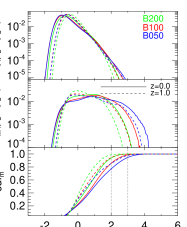
Figure 2: Top: The volume fraction of baryonic matter as a function of density contrast in the three simulations mentioned in section 2 at $z=1$ and $z=0$; the bin width is $\Delta[\mathrm{log(\rho_{b}/<\rho_{b}>)]=0.05}$, and $<\rho_{b}>$ indicates the cosmic mean density of baryon. Middle: The mass fraction of baryonic matter in three simulations. Bottom: The cumulative distribution of baryon mass fraction as a function of density contrast.

2.2 Calculation of DM and scattering

For a source at redshift $z_{s}$, the dispersion measure caused by the IGM and accounting for the frequency shift due to cosmic expansion is(McQuinn 2014; Deng & Zhang 2014)

$${\rm{DM}}(z_{s})=\int_{0}^{z_{s}}\frac{n_{e}(z)}{1+z}dl,$$ (1)

where $n_{e}(z)$ is the number density of electrons at redshift $z$. The effective scattering measure because of the extended IGM is given by (e.g., MK13 and XZ16)

$${\rm{SM}}_{\rm{eff}}(z_{s})=\int_{0}^{z_{s}}\frac{C_{N}^{2}(z)d_{H}(z)}{(1+z)^{3}}dz,$$ (2)

where $d_{H}(z)=cH_{0}^{-1}[\Omega_{\Lambda}+\Omega_{m}(1+z)^{3}]^{-1/2}$ is the Hubble radius, and $C_{N}^{2}(z)$ is related to the variance of electron density $\langle\delta n_{e}^{2}(z)\rangle$ as

$$C_{N}^{2}(z)\approx\frac{\beta-3}{2(2\pi)^{4-\beta}}\langle\delta n_{e}^{2}(z)\rangle L_{0}^{3-\beta}$$ (3)

when the density power spectrum of the turbulence follows a power law with index $\beta>3$(see XZ16 for $\beta<3$) between the outer scale $L_{0}$ and the inner scale $l_{0}$, assuming $l_{0}\ll L_{0}$. Although there are both supersonic and subsonic turbulence in the IGM (Z13, Vazza et al. 2017), we only consider the latter and adopt the Kolmogorov turbulence model, i.e., $\beta=11/3$. Following MK13, we take $\langle\delta n_{e}^{2}(z)\rangle\sim n_{e}^{2}(z)$ , i.e., assuming that the IGM are fully ionized. By and large, the IGM became nearly fully ionized after the reionization era, i.e., $z\lesssim 5.5$. A small fraction of IGM remain neutral, which we will not take into account it in this work for the sake of simplicity. Then, the effective scattering measure is

$${{\rm{SM}}_{\rm{eff}}}(z_{s})\approx 1.42\times 10^{-13}\left(\frac{\Omega_{b}}{0.049}\right)^{2}\left(\frac{L_{0}}{1\rm{pc}}\right)^{-2/3}$$ (4)

$${\rm{m}}^{-20/3}\times\int_{0}^{z_{s}}[\rho_{b}(z)/\bar{\rho}_{b}(z)]^{2}(1+z)^{3}d_{H}(z)dz$$

$$\approx 1.31\times 10^{13}\ {\rm{m}}^{-17/3}\cdot\frac{1}{h}\ \left(\frac{\Omega_{b}}{0.049}\right)^{2}\left(\frac{L_{0}}{1\rm{pc}}\right)^{-2/3}$$

$$\times\int_{0}^{z_{s}}\left[\rho_{b}(z)/\bar{\rho}_{b}(z)\right]^{2}\frac{(1+z)^{3}}{[\Omega_{\Lambda}+\Omega_{m}(1+z)^{3}]^{1/2}}dz.$$

Using conventional methods (e.g., Gnedin & Jaffe 2001; Dolag et al. 2015), we stack the simulation volumes and construct light-cones to calculate ${\rm{DM}}(z_{s})$ and ${\rm{SM_{eff}}}(z_{s})$.

3 Contributions to DM and SM by the IGM in the cosmic web

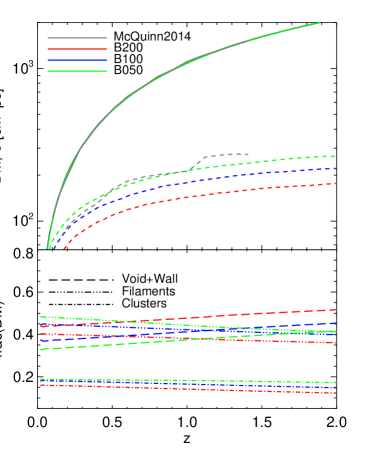
Figure 3: Top: The solid lines indicate the mean values of DM caused by the IGM as a function of the redshift, whereas the dashed lines show the standard deviations. The gray lines represent the result in McQuinn 2014. The red and blue lines are the results in this work based on simulations B200 and B100, respectively. Bottom: The dotted-dashed, triple-dotted-dashed, and long dashed red lines indicate the fractions of DM contributed by the gas in clusters, filaments, and voids and walls, respectively.

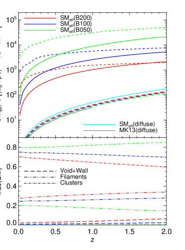
Figure 4: Top: the solid (short dashed) lines indicate the mean values (standard deviations) of ${\rm{SM}_{eff}}(z)$ caused by the IGM as a function of the redshift; the blue, red and green lines indicate the results based on simulations B200, B100 and B050, respectively. The long dashed lines show ${\rm{SM}_{eff}}(z)$ caused by gas in voids and walls. The gray and cyan solid lines indicate ${\rm{SM}_{eff}}(z)$ caused by the diffuse IGM in MK13 and this work, respectively. Bottom: identical to the bottom panel of Figure 3 but for ${\rm{SM}_{eff}}(z)$.

We randomly sampled 10000 lines of sight for each cosmological simulation. The mean value of ${\rm{DM}}$ contributed by the IGM as a function of redshift $z$, i.e., ${\rm{DM_{IGM}}}(z)$, and the corresponding standard dispersion at $z<2$ are shown by solid and short-dashed lines, respectively, in the top panel of Figure 3. Our results for ${\rm{DM_{IGM}}}(z)$ are consistent with McQuinn (2014) in all three simulations. The deviation in B050 is almost consistent with those of McQuinn (2014). However, in the other two simulations, the deviations are relatively smaller, which may be a result of the relatively poorer resolution compared to the simulation sample in McQuinn (2014), which has a mass resolution of dark matter particles of $3\times 10^{7}h^{-1}M_{\odot}$, and a softening length of 1.6 $h^{-1}$ kpc. Increasing the resolution helps to resolve large density fluctuations in the over-dense region.

The baryonic gas resides in different cosmic structures, i.e., voids, walls, filaments and clusters. To probe the contributions to ${\rm{DM_{IGM}}}(z)$ of different structures, the grid cells are assigned to four categories of structures as in Zhu & Feng (2017). As shown in the lower panel of Figure 3, the gas in clusters contributes approximately $\sim 15\%-20\%$ of the total ${\rm{DM}_{eff}}(z)$, the gas in filaments contributes $\sim 35-45\%$, and the gas in voids and walls contribute the remaining $\sim 35-45\%$.These fractions basically trace the mass distribution of baryonic matter in the cosmic web as demonstrated in Zhu & Feng (2017).

MK13 analytically estimated the effective SM due to the extended, diffuse IGM by assuming that the IGM had an isotropic and uniform distribution and concluded that it was weak. We run the identical estimation by taking $\rho_{b}(z)/\bar{\rho}_{b}(z)=1$ in eqn. (4) and denote it as ${\rm{SM}_{eff,diff}}(z)$. As shown in the top panel of Figure 4, our result for ${\rm{SM}_{eff,diff}}(z)$ is $\sim 1.5$ times that in MK13, which should be caused by different cosmological parameters. Then, we derive the mean effective scattering measure as a function of the redshift, i.e., ${\rm{SM}_{eff}}(z)$, based on the IGM distribution in our simulations, which is shown as the red, blue and green solid lines in Figure 4. The mean value of ${\rm{SM}_{eff}}(z)$ in B200 is approximately 20 times larger than ${\rm{SM}_{eff,diff}}(z)$. It is approximately $10^{15}(L_{0}/\rm{1pc})^{-2/3}\,\rm{m}^{-17/3}$, i.e., $3.25\times 10^{-5}(L_{0}/\rm{1pc})^{-2/3}\,\rm{kpc}\,\rm{m}^{-20/3}$, at $z=1$ in B200. The corresponding ${\rm{SM}_{eff}}$ in B100 and B050 increases by a factor of 2.5 and 10, respectively, compared with B200. For an out scale of $L_{0}\sim 100\,$kpc, which was adopted in some previous work(Luan & Goldreich 2014, XZ16), ${\rm{SM}_{eff}}$ in B050 is approximately $5\times 10^{12}\,\rm{m}^{-17/3}$ at $z=1$. Apparently, the outer scale influences whether scattering in the IGM/clusters is important or not. We will probe this effect in the next section.

The short dashed lines in the top panel of Figure 4 indicate the corresponding dispersions of ${\rm{SM}_{eff}}(z)$. Consistent with the speculation in MK13, ${\rm{SM}_{eff}}(z)$ shows significant LOS variations with a larger standard deviation than $2$ times the mean value at $z\leq 0.5$ in all simulations. We also found that a higher simulation resolution corresponds to larger LOS variations in ${\rm{SM}_{eff}}(z)$. These dramatic variations are expected to weaken the dependence of ${\rm{SM}_{\rm{IGM}}}$ on ${\rm{DM}_{\rm{IGM}}}$ if the sample size is small. The excess of ${\rm{SM}_{eff}}(z)$ with respect to ${\rm{SM}_{eff,diff}}(z)$ and the dramatic LOS variations should result from the intervention of filaments and clusters along some LOS. The long dashed lines in the top panel of Figure 4 indicate that the effective SM caused by gas in voids and walls is close to the value of ${\rm{SM}_{eff,diff}}(z)$ and contributes only $\sim 4\%-5\%$ of the total ${\rm{SM}_{eff}}(z)$. The gas in clusters and filaments contributes approximately $65-80\%$ and $20-30\%$, respectively, as shown in the lower panel of Figure 4. The absolute magnitude of the effective SM contributed by the gas in clusters is significantly higher than the estimated value in MK13. Moreover, the contribution by the gas in clusters is relative higher in B050 than in B100 and B200. The increase in ${\rm{SM}_{eff}}$ in B050 should primarily result from the stronger density fluctuation in the cluster region captured by the increased spatial resolution. As Figure 2 demonstrated, there are more cells that have a baryon density $\rho_{b}/\bar{\rho}_{b}>10$ in B050 with respect to B200 and B100. According to eqn. 4., the magnitude of ${\rm{SM}_{eff}}$ would be very sensitive to such cells, for a fixed $L_{0}$. Those cells are likely belong to filaments and clusters, considering the density distribution in the cosmic web (Zhu & Feng 2017).

In short, the gas in clusters contributes only $15\%$ of ${\rm{DM_{IGM}}}$ but dominates the effective SM caused by the IGM.

4 Time broadening of FRBs by the IGM

In this section, we study the time broadening of FRBs due to the reported effective scattering measure of the IGM in the last section. For comparison with observations, we use the information of the observed FRBs with available scattering times. More specifically, we include 17 events compiled in Cordes et al. (2016) and Y17, 4 events reported in Bhandari et al. (2018), event FRB 150807(Ravi et al., 2016) and event FRB 170107(Bannister et al., 2017). Many previous theoretical studies investigated the broadening by the IGM at $\sim 300$ MHz (e.g., MK13 and Luan & Goldreich 2014 ). However, the time broadening of the observed FRBs is commonly measured and provided at approximately $\sim 1$ GHz(Petroff et al. 2016). Thus, for a more accurate comparison between our result and the observational results, we discuss the time broadening at 1 GHz.

4.1 Variations, dependence on DM, and strength

The relation between the temporal broadening and $\rm{SM}_{\rm{eff}}$ for Kolmogorov turbulence is (e.g., MK13)

$$\tau=10^{-4}\ {\rm{ms}}\times(1+z_{L})^{-1}\left(\frac{D_{\rm{eff}}}{1\rm{Gpc}}\right)\times$$ (5)

$$\left\{\large\begin{array}[]{ll}3.32\times\left(\frac{\lambda_{0}}{30\rm{cm}}\right)^{4}\left(\frac{\rm{SM}_{\rm{eff}}}{10^{12}\rm{m}^{-17/3}}\right)\left(\frac{l_{0}}{1\rm{AU}}\right)^{-\frac{1}{3}}&r_{\rm{diff}}<l_{0}\vspace{3mm}\\ 9.50\times\left(\frac{\lambda_{0}}{30\rm{cm}}\right)^{\frac{22}{5}}\left(\frac{\rm{SM}_{\rm{eff}}}{10^{12}\rm{m}^{-17/3}}\right)^{\frac{6}{5}}&r_{\rm{diff}}>l_{0}\end{array}\right.$$

where $z_{L}$ is the redshift of the scattering matter; $\lambda_{0}$ is the wavelength in the observer’s frame; $D_{\rm{eff}}=D_{L}D_{S}/D_{LS}$, with $D_{L}$ and $D_{S}$ being the angular diameter distance of the scattering matter and the source from the observer, respectively; and $D_{LS}$ is the angular diameter distance of the source from the scattering matter. The diffractive length scale $r_{\rm{diff}}$ for $\beta=11/3$ is approximately

$$r_{\rm{diff}}\sim(\pi r^{2}_{e}\lambda^{2}_{0}\rm{SM}_{\rm{eff}}\mathit{l}_{0}^{-\frac{1}{3}})^{-1/2},r_{\rm{diff}}<\mathit{l}_{0},$$ (6a)

$$r_{\rm{diff}}\sim(\pi r^{2}_{e}\lambda^{2}_{0}\rm{SM}_{\rm{eff}})^{-3/5},r_{\rm{diff}}>\mathit{l}_{0}.$$ (6b)

As shown in eqns. (4) and (5), $\tau_{\rm{IGM}}$ highly depends on $L_{0}$ and $l_{0}$. Although significant density fluctuations of gas were found on the resolution scale, i.e., tens of kpc, in many simulations with or without star formation and AGN, it remains a challenge to probe them by observation. Density fluctuations on similar scales in the central region of the Coma and Perseus clusters were recently reported (Churazov et al. 2012; Zhuravleva et al. 2015). However, constrained by resolution, both simulation and observation cannot provide any information between tens of kpc and the Fresnel scale, i.e., $\sim$ 10 AU. Thus, the value of $\tau_{\rm{IGM}}$ discussed here is based on certain assumptions on $L_{0}$ and $l_{0}$.

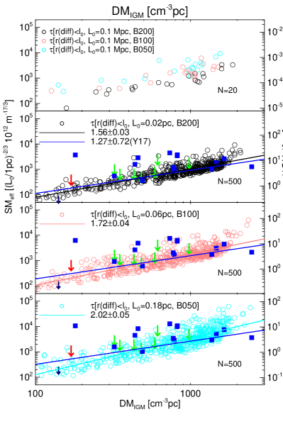
Figure 5: $\rm{SM}_{\rm{eff}}$($\tau_{\rm{IGM}}$) as a function of $\rm{DM_{IGM}}$. Top panel: The left axis shows the $\rm{SM}_{\rm{eff}}$ of 20 mock sources, and the right axis indicate the corresponding $\tau_{\rm{IGM}}$ at $\nu=1\,$ GHz for the case $r_{\rm{diff}}<l_{0}$ and $L_{0}=0.1$Mpc. From the second to fourth panels: The circles indicate the $\rm{SM}_{\rm{eff}}$ and $\tau_{\rm{IGM}}$ of 500 mock sources in B200, B100 and B050(the value of $L_{0}$ is adjusted for each simulation, see the text for details). The solid black, pink and cyan lines indicate the linear fitting results of $\tau_{\rm{IGM}}\propto\rm{DM}_{\rm{IGM}}^{n}$, and the blue solid lines indicate the fitting in Yao et al. (2017). The $\tau$ and $\rm{DM}_{\rm{IGM}}$ of the observed events (filled square and downward arrow) are given by data in relevant references(see Petroff 2016). The red arrow indicates the repeating FRB 121102. The navy blue arrow indicates the event FRB150807, which has been shifted upward by an order of magnitude.

For simplicity, we first consider the case $r_{\rm{diff}}<l_{0}$ with $l_{0}\approx 1$AU and assume that $(1+z_{L})\sim 1,D_{\rm{eff}}\sim 1{\rm{Gpc}}$. For the stacked IGM distribution of each cosmological simulation, we randomly place 20 mock sources in the redshift range $0.10<z<1.50$. The top panel in Figure 5 shows $\rm{SM}_{eff}$ as a function of $\rm{DM}_{\rm{IGM}}$ of these mock sources. The low- and high-redshift ends of mock sources are selected so that ${\rm{DM}}$ $(z_{\rm{low}})$ and ${\rm{DM}}$ $(z_{\rm{high}})$ in section 2 are approximately equal to the smallest and largest $\rm{DM}_{\rm{IGM}}$ of the observed FRBs. In fact, both host galaxies and the IGM can contribute to the DM of the observed events. Various models have been introduced in the literature, but the actual picture remains unclear. So far, it is not straightforward to determine the $\rm{DM}_{\rm{IGM}}$ of observed FRBs using any method. As a beginning, we use a notably simple model following Yao et al. (2017), i.e., assuming that the hosts’ contribution to DM is $\rm{DM}_{host}=100\,\rm{pc\,cm^{-3}}$, except for the repeating event FRB 121102. This simplification can help us to reveal the dependence of $\tau_{\rm{IGM}}$ on factors such as $\rm{DM}_{\rm{IGM}}$ and simulation resolution. The host galaxy’s contribution for FRB 121102 is set to $\rm{DM}_{host}=170\,\rm{pc\,cm^{-3}}$ according to recent observations(Spitler et al. 2016; Chatterjee et al. 2017; Tendulkar et al. 2017; Bassa et al. 2017). The assumption of $\rm{DM}_{host}=100\,\rm{pc\,cm^{-3}}$ is likely oversimplified, so we will consider more realistic models in the next subsection.

The dependence of $\tau$ on ${\rm{DM}}$ is used as an important indicator to determine whether the IGM is an important scattering matter of FRBs. For a given $L_{0}$, the dependence of $\tau_{\rm{IGM}}$ on ${\rm{DM_{IGM}}}$ for these 20 mock sources is weak for all three simulations. The lack of a strong dependence results from the large LOS variations and limited sample size. The variations in $\tau_{\rm{IGM}}$ can be up to $\sim 1$ orders of magnitude at $\rm{DM_{IGM}}\sim 1000\,\rm{pc\,cm^{-3}}$. We then increase the number of randomly distributed mock sources to 500 for the stacked IGM distribution of each simulation, while the redshift range is kept to $0.10<z<1.50$. The second to fourth panels in Figure 5 show that with a largely increased sample size of 500, $\tau_{\rm{IGM}}$ shows a clear positive correlation with ${\rm{DM_{IGM}}}$. The linear least square fitting gives $\tau_{\rm{IGM}}\propto{\rm{DM_{IGM}}}^{1.56\pm 0.03}$, ${\rm{DM_{IGM}}}^{1.72\pm 0.04}$, and ${\rm{DM_{IGM}}}^{2.02\pm 0.05}$ in the three simulations. The linear Pearson correlation coefficient of $\mathrm{log(\tau_{IGM})}$ and $\mathrm{log(DM_{IGM})}$ are $0.90,0.88,0.87$ in B200, B100, and B050 respectively. The scaling relation in our work are steeper than the result in Yao et al. (2017), i.e., $\tau\propto{\rm{DM_{IGM}}}^{1.27\pm 0.72}$, but are within their range of scatter. This discrepancy may be alleviated if the real $\tau$ of those observed FRBs with only upper limits is smaller than the limits. In addition to the large LOS variations of $\rm{SM}_{eff,IGM}$, the dependence of $\tau$ on ${\rm{DM}}$ is also complicated by the mixing contribution to the DM by both the host galaxy and IGM. Meanwhile, the selection effect of observed events is not clear. Thus, in contrast to Katz (2016), the observed non-monotonic dependence of the widths of FRBs on DM cannot be used as solid evidence to rule out the IGM considering the limited number of events.

The magnitude of $\tau_{\rm{IGM}}$ is another important criterion to evaluate the contribution of the IGM to the broadening of FRBs. According to the estimated value of $\rm{SM}_{\rm{eff}}$ in section 2, $\tau_{\rm{IGM}}$ is $\sim 10^{-4}-10^{-3}(10^{-2}-10^{-1})\,$ ms at the frequency of $1\,$ GHz(300MHz) for ${\rm{DM_{IGM}}}\sim 1000\,\rm{pc\,cm^{-3}}$, with an outer scale of $L_{0}\sim 100\$kpc. This level is implausible for explaining the observed events with $\tau\sim 5\,$ms at $\nu\sim 1$ GHz. We then adjust the value of $L_{0}$ in the calculation of $\rm{SM_{eff}}$ for each simulation sample, to make $\tau_{\rm{IGM}}{\rm{(1\,GHz)}}\sim 1-10\,$ms for $\rm{DM_{IGM}}\sim 500-1000\,\rm{pc\,cm^{-3}}$. A significantly smaller $L_{0}$ on the order of $\sim 0.02$pc is required in B200, as shown in the second plot of Figure 4. The required $L_{0}$ can be increased to $\sim 0.06,0.18\$pc in B100 and B050, respectively, because of the stronger density fluctuations captured by the increased resolution. For such values of the outer scale, the distribution of $\tau_{\rm{IGM}}-\rm{DM_{IGM}}$ of mock sources can nearly cover that of the observed events, except for FRB010724 and FRB160102. For the former event, we will revisit it later. The event FRB 160102 with the highest $\rm{DM}_{xg}$ could be covered by an increased high-redshift end.

Figure 6 shows the case with $r_{\rm{diff}}>l_{0}$. For $\rm{DM}_{\rm{IGM}}\sim 500-1000\,\rm{pc\,cm^{-3}}$, the required outer scale $L_{0}$ to produce $\tau_{\rm{IGM}}{\rm{(1\,GHz)}}\sim 1-10\,$ms is $\sim 5\,$pc in B050, which is relatively larger than the case with $r_{\rm{diff}}<l_{0}$. Meanwhile, convergence with increasing resolution is not attained in B050. The demanded outer scale of turbulence is expected to further increase with increasing resolution.

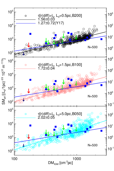
Figure 6: Identical to the bottom three panels in Figure 5 but for $r_{\rm{diff}}>l_{0}$.

4.2 $\tau_{\rm{IGM}}-DM_{\rm{IGM}}$ relation: the key role of the gas in the clusters

Assuming that the mock sources are randomly distributed in a certain redshift range, the dependence of $\tau_{\rm{IGM}}$ on ${\rm{DM_{IGM}}}$ in our simulations tends to steepen when the resolution increases. This trend should be related to the enhanced density fluctuations in simulations with higher resolution, particularly in the clusters. We probe this effect by calculating the broadening time due to the effective measure caused by gas in different structures. We use the same mock sources as in the last subsection. In Figure 7, the horizontal axis indicates the dispersion measure contributed by gas in voids and walls, filaments, and clusters. The vertical axes indicate the corresponding effective scattering measure and broadening time, assuming $r_{\rm{diff}}<l_{0}$. To isolate the impact of resolution on $\rm{SM}_{\rm{eff}}$, as well as the dependence of $\tau_{\rm{IGM}}$ on ${\rm{DM_{IGM}}}$, we use an identical outer scale of $L_{0}=0.18\,$ pc for all the samples from three simulations in this subsection.

The top panel shows that the relation between $\tau$ and DM due to the extended, diffuse IGM in voids and walls is consistent in the three simulations, with $\tau_{\rm{void}}\propto{\rm{DM_{IGM,void}}}^{1.36-1.38}$ with small scatter. Discrepancies appear in the case of gas in filaments, with $\tau_{\rm{filament}}\propto{\rm{DM_{IGM,filament}}}^{1.38}$, $\propto{\rm{DM_{IGM,filament}}}^{1.54}$, and $\propto{\rm{DM_{IGM,filament}}}^{1.68}$ in B200, B100 and B050, respectively. Evident dispersion also appears and is enhanced by the increased resolution. The scaling relation between $\tau$ and $\rm{DM}$ by the baryonic matter in the clusters is the steepest, with $\tau_{\rm{cluster}}\propto{\rm{DM_{IGM,cluster}}}^{1.64}$, $\propto{\rm{DM_{IGM,cluster}}}^{1.76}$, and $\propto{\rm{DM_{IGM,cluster}}}^{2.00}$ in the three simulations.

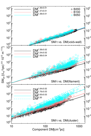
Figure 7: Top: The dispersion measure and effective scattering measure caused by the gas residing in voids and walls and the corresponding $\tau$, assuming $r_{\rm{diff}}<l_{0}$ and $L_{0}=0.18$ pc; the black, pink and cyan circles indicate the mock sources in simulations B200, B100 and B050, respectively. Middle (bottom): identical to the top panel but for those caused by the gas in filaments (clusters).

In section 3, we find that the baryons in the clusters dominates the scattering measure and contributes approximately $15\%$ of the dispersion measure due to the IGM. Hence, the global relation between $\tau_{\rm{IGM}}$ and $\rm{DM}_{\rm{IGM}}$ should be largely determined by the scaling of $\tau_{\rm{cluster}}-{\rm{DM_{IGM,cluster}}}$. Figure 8 presents an example based on simulation B050. This property can explain the result of the global scaling relation obtained in the last subsection. The scaling relation of $\tau\propto{\rm{DM^{2.00}}}$ is consistent with some previous analysis for a homogeneous turbulent scattering medium (e.g., see Cordes et al. 2016 ). Meanwhile, it is shallower than the scaling relation of the observed Galactic pulsars at $\rm{DM}>100\,\rm{pc\,cm^{-3}}$. Cordes et al. (2016) showed that the mean scattering time of the observed pulsars could be fitted by

$$\widehat{\tau}(\rm{DM})=2.98\times 10^{-7}\times{\rm{DM}}^{1.4}\times$$ (7)

$$(1+3.55\times 10^{-5}\times{\rm{DM}}^{3.1})\,{\rm{ms}}.$$

As there are no signs of convergence in our simulations, the dependence may become more steep if the resolution is further increased. On the other hand, the density fluctuations in the clusters are probably more homogeneous than those in the interstellar medium of the Milky Way and result in a relatively shallower scaling relation. Other physical properties, such as the thermal and ionization states, are likely different between the ISM in the Milky Way and IGM, including the baryonic medium in clusters. Hence, the scattering law of Galactic plasma may be not applicable to the scattering in the IGM.

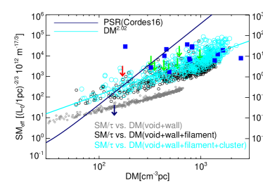
Figure 8: Effective scattering measure and the corresponding $\tau$ as a function of the dispersion measure in simulation B050 with $r_{\rm{diff}}<l_{0}$ and $L_{0}=0.18$ pc. The gray circles indicate the value contributed by gas in the voids and walls. The black circles indicate the value contributed by the IGM, excluding those in clusters. The cyan circles indicate the values contributed by the IGM in all structures.

4.3 Dispersion and scattering by the host galaxy and IGM

The assumption of $\rm{DM}_{\rm{host}}=100\,\rm{pc\,cm^{-3}}$ in section 4.1 is likely oversimplified and may overestimate the redshift of FRB events. Cordes et al. (2016) discussed a set of mixed models in which the dispersion and scattering of FRBs involved both the host galaxy and the IGM and suggested that the extragalactic portion of the FRBs’ DM, i.e., $\rm{DM}_{xg}$, either consisted of mixture contributions or was dominated by the host. The scenario that the host galaxy dominated the broadening was favored in the literature, as the studies mainly considered the diffuse IGM, which has a relatively lower density. Our results based on simulations indicate that the gas in the filaments and clusters may play an important role, which is consistent with the speculation in MK13. Hence, there may be other possible solutions, e.g., the broadening of some events is dominated by the host, whereas other events are dominated by the intervention of clusters and filaments.

In the upper and lower panels of Figure 9, the host’s contributions to the $\rm{DM}_{xg}$ of the observed events are set to $50\%$ and $20\%$, respectively, close to one of the mixed models proposed in Cordes et al. (2016). The cyan lines indicate the expected $\tau_{\rm{host}}$ due to $\rm{DM}_{host}$ according to the scaling law of $\tau_{\rm{host}}-{\rm{DM}_{host}}$, which was derived from the observed pulsars in Cordes et al. 2016. The circles indicate mock sources randomly distributed in the redshift ranges of $0.10<z<0.75$ and $0.10<z<1.35$ based on simulation B050. $\tau_{\rm{IGM}}$ is obtained according to eqn. 5a assuming $L_{0}=0.18\$pc. In the top panel, the expected $\tau_{\rm{host}}$ can well explain several events in the top-left region of the $\tau-\rm{DM}$ space, except for FRB010724. With the fraction of the DM contributed by the host galaxy larger than $50\%$, the scaling law in Cordes et al. 2016 can explain this event. However, the remaining events show an evident scattering deficit with respect to $\tau_{\rm{host}}$. Decreasing the host’s contribution to $\rm{DM}_{xg}$, as in the bottom panel, can resolve the deficit. In other words, both the DM and $\tau$ of those events can be primarily contributed by the IGM if $L_{0}\sim 0.18\$pc for $r_{\rm{diff}}<l_{0}$ or $L_{0}\sim 5\$pc for $r_{\rm{diff}}>l_{0}$. Alternatively, if the host galaxy dominates the scattering while the IGM dominate the DM can also explain those events.

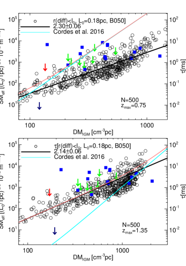
Figure 9: Same as Figure 5, but the $\rm{DM}_{IGM}$ of observed events is set to $50\%$ and $80\%$ of the $\rm{DM}_{xg}$ in the top and bottom panels, respectively. The cyan lines indicate the expected $\tau_{host}$ according to the scaling law given in Cordes et al. (2016). The red lines indicate the sum of $\tau_{host}$ and fitted $\tau_{\rm{IGM}}$.

5 Discussion

To make $\tau_{\rm{IGM}}\sim 5\,$ms at $\nu=1\,$GHz, the required $L_{0}$ here is $\sim 2.5$ orders higher than the value of $10^{-3}-10^{-2}\,$pc in the literature(Luan & Goldreich 2014, XZ16). Moreover, the estimated broadening times in many theoretical works were at the frequency $\nu=0.3$ GHz. To produce $\tau_{\rm{IGM}}\sim 5\,$ms at $\nu=0.3\,$GHz, the required $L_{0}$ in B050 can be as large as 3.6 kpc if $r_{\rm{diff}}>l_{0}$ or 250 pc if $r_{\rm{diff}}<l_{0}$. Namely, the required $L_{0}$ can be $\sim 5$ orders higher than the values reported in previous investigations. The latter were evaluated from the diffuse IGM in voids and walls with $\rho_{b}/\bar{\rho}_{b}\sim 1$, whereas our results are based on the clumpy IGM in simulation, which is mainly contributed by the gas in filaments and clusters. Luan & Goldreich (2014) stated that the dissipation of turbulence with a notably small outer scale might double the temperature of the IGM on an extremely short timescale and would be incompatible with the cooling timescale, which is comparable to the Hubble time $t_{H}$. The heating timescale $\tau_{\rm{heat}}$ is approximately (XZ16)

$$\tau_{heat}\sim\frac{L_{0}}{c_{s}}=200(\frac{L_{0}}{10^{-2}\rm{pc}})(\frac{T}{10^{5}\rm{K}})^{-\frac{1}{2}}\rm{yr},$$ (8)

where $c_{s}$ is the speed of sound. If $L_{0}=10^{-2}$pc, $\tau_{\rm{heat}}$ is $\sim 200\,\rm{yr}$ for gas with $T=10^{5}$K, which is much shorter than $t_{H}$. The required $L_{0}\sim 5\,$pc here can increase $\tau_{\rm{heat}}$ to $\sim 10^{5}\,$yr but remains significantly shorter than $t_{H}$.

This tension may be further alleviated when we consider the distribution of turbulence. The turbulence in the IGM is only well developed in the over-dense region. Hence, the turbulence heating is a local effect and will not change the global thermal history of the IGM, particularly the diffuse IGM in the voids and walls. Moreover, for the warm-hot ($10^{5}<T<10^{7}$K) gas in the over-dense region, the median ratio of turbulent kinetic energy to thermal energy was approximately $\sim 0.3$ in the adaptive mesh refined cosmological hydrodynamic simulations (e.g., Schmidt et al. 2017). Hence, turbulent heating is not expected to dramatically change the temperature. For the cold gas ($T<10^{5}$K) in the over-dense region, the cooling will be largely accelerated by the metal enrichment (Smith et al. 2008).

However, the required $L_{0}\sim 5\,$pc to produce $\tau_{\rm{IGM}}\sim 5\,$ms at $\nu=1\,$GHz is much smaller than the resolution of our simulations, and remains significantly smaller than the turbulence injection scale associated with cosmic structure formation, i.e., $\gtrsim 0.1$ Mpc, according to cosmological simulations(Ryu et al. 2008; Z13). The upper end scale of the inertial range of Kolmogorov turbulence is usually $0.5$ dex smaller than the injection scale (Porter et al. 1998), which may shorten the gap to 4 orders of magnitude. In addition, we find that the effective SM and required $L_{0}$ increase by a factor of $\sim 3$ when the spatial resolution of simulation increases by a factor of 2, because of improved capability to resolve over-dense region. On the other hand, increasing resolution can help to resolve less massive objects and their motions, and inject turbulence on scale smaller than current simulations. Thus, the gap may be significantly reduced if the simulation resolution is further increased, which, however, would require massive computational resources.

While a convergence result is currently unavailable in this work, previous simulations and observations in the literature can provide some hints on the potential capability of shorten the gap by increasing resolution further. Figure 2 indicates that, for a fixed $L_{0}$, the increment on $\rm{SM_{eff}}$ in simulation with higher resolution results mainly from increased fraction of cells with baryonic density $\rho_{b}(z)/\bar{\rho}_{b}(z)>100$. At $z=0$, the mass fraction of baryonic matter with $\rho_{b}/\bar{\rho}_{b}>100$ is $\sim 25\%$ in B050, which is smaller than a fraction of $\sim 35\%$ in Dave et al. (2010) based on a simulation with spatial resolution $\sim 5$ kpc. The mass fraction with $\rho_{b}/\bar{\rho}_{b}>1000$ is about $\sim 2\%$ and $\sim 5\%$ at $z=1$ and $z=0$ respectively in B050, which is smaller than $\sim 9\%$ and $\sim 8\%$ respectively in Vogelsberger et al. (2012) based on a moving-mesh cosmological simulation with resolution of a few kpc. So far, the density fluctuation in the IGM on and below $\sim 10\,$kpc has not resolved by observations. Nevertheless, many observational efforts have been made to probe the properties of multi-phase IGM at low redshifts(e.g., Shull et al. 2012, Werk et al. 2014, Danforth et al. 2016). These studies suggested that about $30\%$ of the cosmic baryonic matter was likely in the state of diffuse photoionized IGM with $\rho_{b}/\bar{\rho}_{b}<100$ and $T<10^{5}$ K, based on observation of low redshift Lyman-$\alpha$ forest. Another $\sim 30\%$ was in the phase of shock heated warm-hot intergalactic medium with $\rho_{b}/\bar{\rho}_{b}<100$ and $T>10^{5}$ K based on observation of O VI and broad Lyman absorbers. The remaining $\sim 40\%$ may reside in collapsed objects and circumgalactic gas with baryon density $\rho_{b}/\bar{\rho}_{b}>100$, and is still under investigation. In short, the mass fraction with $\rho_{b}/\bar{\rho}_{b}>100$ in the highest resolution simulation B050 in our work is lower than the results reported in the literature. The mismatch between the required $L_{0}$ and turbulence injection scale is expected to be alleviated by increasing resolution.

Last but not the least, if future observations find that the IGM indeed plays an important role in the scattering of FRBs, it may help to probe the gas in filaments and clusters.

6 Conclusions

Using cosmological hydrodynamical simulations, we investigate the dispersion and scattering of FRBs caused by the IGM. The mean value of dispersion measure contributed by the IGM as a function of redshift $z$ in our work is in well agreement with the literature(e.g., McQuinn 2014). Moreover, we probe the contribution to $\rm{DM}_{\rm{IGM}}$ by the gas residing in various structures of the cosmic web. We find that the gas in clusters contributes approximately $\sim 15\%-20\%$ of the total dispersion measure caused by the IGM, the gas in filaments contributes $\sim 35-45\%$, and the gas in voids and walls contribute the remaining $\sim 35-45\%$. We confirm that the scattering by the clumpy IGM has significant LOS variations. We show that the scattering of FRBs by the IGM in voids and walls is weak, but the medium in clusters and filaments can enhance the scattering by a factor of 200 in our simulation with the highest resolution. Specifically, the gas in clusters contributes approximately $65-80$% of the total SM caused by the IGM, while gas in filaments contributes $20-30$%. We argue that the observed non-monotonic dependence of the widths of FRBs on DMs cannot determine whether the IGM is an important scattering matter of FRBs or not, considering the significant LOS variations, limited number of observed events and mixing contribution to the DMs by the host galaxy and IGM.

Under the assumption of turbulence following Kolmogorov scaling, an outer scale of $\sim 5$pc is required to make $\tau_{\rm{IGM}}$ reach $\sim 1-10\,$ms at 1 GHz to explain the observed events with $\tau\geq 1\,$ms. This outer scale can significantly alleviate the tension regarding the timescale of turbulent dissipation and IGM cooling but remains approximately 4 orders of magnitude lower than the currently estimated turbulence injection scale due to structure formation. We find that the estimated effective scattering measure in our simulation is notably sensitive to the simulation resolution. With a higher resolution, stronger density fluctuations can be resolved. The gap in the outer scale of turbulence may be effectively shortened if the simulation resolution can be enhanced. With a mock sample of 500 sources evenly distributed in the redshift range of $0.1<z<1.5$, the dependence of $\tau_{\rm{IGM}}$ on $\rm{DM}_{\rm{IGM}}$ is $\tau_{\rm{IGM}}\propto\rm{DM_{IGM}}^{1.56-2.02}$. The upper value of the scaling index, i.e., 2.02, is determined by the gas in clusters.

Factors including feedback from star formation and AGN, and supersonic turbulence may further decrease the gap in the outer scale. Feedback processes can drive the density fluctuations below tens of kpc. The density fluctuation of supersonic turbulence differs from that of subsonic turbulence, which may change the required scales (see XZ16). Meanwhile, effects such as $z_{L}$ and $D_{\rm{eff}}$ have not been considered, which makes our results for $\tau_{{\rm{IGM}}}$ somewhat overestimated. The selection effect and intrinsic redshift distribution of the FRBs remain unclear. Finally, the contributions from both the IGM and host galaxies may play important roles in the scattering of FRBs. Namely, the IGM in filaments and clusters may dominate the scattering of some FRBs, whereas the host galaxy dominates others. As the number of observed events continues increasing, the dependence of $\tau$ on DM may help to ascertain the relative contributions from the host galaxy and IGM. A more comprehensive investigation will be conducted in the future to cover these factors.

References

- Abramson et al. (2011) Abramson, A., Kenney, J. D. P., Crowl, H. H., Chung, A., van Gorkom, J. H., et al., 2011, ApJ, 141, 164
- Bannister et al. (2017) Bannister, K. W., Shannon, R. M., Macquart, J.-P., Flynn, C., Edwards, P. G, et al., 2017, ApJL, 841, 12
- Bassa et al. (2017) Bassa, C. G., Tendulkar, S. P., Adams, E. A. K., Maddox, N., Bogdanov, S., et al., 2017, ApJL, 843, 8
- Bhandari et al. (2018) Bhandari,S., Keane, E. F., Barr, E. D., et al., 2018, MNRAS, 475, 1427
- Bond et al. (1996) Bond J. R., Kofman L., Pogosyan D., 1996, Nature, 380, 603
- Champion et al. (2016) Champion, D. J., Petroff, E., Kramer, M., et al., 2016, MNRAS, 460, L30
- Chatterjee et al. (2017) Chatterjee, S., Law, C. J., Wharton, R. S., Burke-Spolaor, S., Hessels, J. W. T., et al., 2017, Nature, 541, 58
- Churazov et al. (2012) Churazov, E., Vikhlinin, A., Zhuravleva, I, Schekochihin, A., Parrish, I., et al., 2012, MNRAS, 421,1123
- Cordes et al. (2016) Cordes, J. M., Wharton, R. S., Spitler, L. G., Chatterjee, S., & Wasserman, I. 2016, arXiv e-prints: 1605.05890
- Danforth et al. (2016) Danforth, C. W., Keeney, B. A., Tilton, E. M., Shull, J. ., Stocke, J. T., et al., 2016, ApJ, 817, 111
- Dave et al. (2010) Dave, R., Oppenheimer, B. D., Katz, N., Kollmeier, J. A., & Weinberg, D. H. 2010, MNRAS, 408, 2051
- Dekel et al. (2009) Dekel, A., Birnboim, Y., Engel, G., Freundlich, J., Goerdt, T., et al., 2009, Nature, 457, 451
- Deng & Zhang (2014) Deng, W., & Zhang, B. 2014, ApJL, 783, L35
- Dolag et al. (2015) Dolag, K., Gaensler, B. M., Beck, A. M., & Beck, M. C., 2015, MNRAS, 451, 4277
- Feng et al. (2004) Feng, L.L., Shu, C.-W., & Zhang, M.P. 2004, ApJ, 612, 1
- Gnedin & Jaffe (2001) Gnedin, N. Y., & Jaffe, A. 2001, ApJ, 551, 3
- Haardt & Madau (2012) Haardt, F., & Madau, P., 2012, ApJ, 746, 125
- Inoue (2004) Inoue, S. 2004, MNRAS, 348, 999
- Ioka (2003) Ioka, K. 2003, ApJL, 598, L79
- Katz (2016) Katz, J. I. 2016, ApJ, 818, 19
- Luan & Goldreich (2014) Luan, J., & Goldreich, P. 2014, ApJ, 785, L26
- Macquart & Koay (2013) Macquart, J.-P., & Koay, J. Y. 2013, ApJ, 776, 125
- Mayer et al. (2006) Mayer, L., Mastropietro, C., Wadsley, J., Stadel, J., & Moore, B. 2006, MNRAS, 369, 1021
- McQuinn (2014) McQuinn, M. 2014, ApJL, 780, L33
- Nelson et al. (2013) Nelson, D., Vogelsberger, M., Genel, S., et al. 2013, MNRAS, 429, 3353
- Lorimer et al. (2007) Lorimer, D. R., Bailes, M., McLaughlin, M. A., Narkevic, D. J., & Crawford, F. 2007, Science, 318, 777
- Ravi et al. (2016) Ravi, V., Shannon, R. M., Bailes, M., Bannister, K., Bhandari, S., et al., 2016, Science, 354, 6317
- Schmidt et al. (2017) Schmidt, W.; Byrohl, C.; Engels, J. F.; Behrens, C.; Niemeyer, J. C., 2017, MNRAS, 470, 142
- Schmidt et al. (2016) Schmidt W., Engels J. F., Niemeyer J. C., & Almgren A. S., 2016, MNRAS, 459, 701
- Shandarin & Zel’dovich (1989) Shandarin, S. F., & Zel’dovich, Ya. B. 1989, RvMP, 61, 185
- Shull et al. (2012) Shull, J. M., Smith, B. D., & Danforth, C. W. 2012, ApJ, 759, 23
- Smith et al. (2008) Smith B., Sigurdsson S., Abel T., 2008, MNRAS, 385, 1443
- Spitler et al. (2016) Spitler, L. G., Scholz, P., Hessels, J. W. T., Bogdanov, S., et al., 2016, Nature, 531, 202
- Petroff et al. (2016) Petroff, E., Barr, E. D., Jameson, A., et al., 2016, PASA, 33, e045
- Planck Collaboration et al. (2014) Planck Collaboration et al., 2014, A&A, 571, 16
- Porter et al. (1998) Porter, D. H., Woodward, P. R., & Pouquet, A. 1998, PhFl, 10, 237
- Ryu et al. (2008) Ryu D., Kang H., Cho J., & Das S., 2008, Science, 320, 909
- Tendulkar et al. (2017) Tendulkar, S. P., Bassa, C. G., Cordes, J. M., Bower, G. C., Law, C. J., et al., 2017, ApJL, 834, 7
- Thornton et al. (2013) Thornton, D., Stappers, B., Bailes, M., et al. 2013, Science, 341, 53
- Vazza et al. (2010) Vazza F., Brunetti G., Gheller C., Brunino R., 2010, NewA, 15, 695
- Vazza et al. (2017) Vazza, F., Jones, T. W., Bruggen, M., Brunetti, G., & Gheller, C., et al., 2017, MNRAS, 464, 210
- Vogelsberger et al. (2012) Vogelsberger, M., Sijacki, D., Kereš, D., Springel, V., Hernquist, L., 2012, MNRAS, 425, 3024
- Werk et al. (2014) Werk, J. K., Prochaska, J. X., Tumlinson, J., Peeples, M. S., Tripp, T. M., et al., 2014, ApJ, 792, 21
- Xu & Zhang (2016) Xu, S., & Zhang, B. 2016, ApJ, 832, 199
- Yao et al. (2017) Yao, J. M., Manchester, R. N., & Wang, N., 2017, ApJ, 835, 29
- Zel’dovich (1970) Zel’dovich, Y. B. 1970, A&A, 5, 84
- Zhu et al. (2010) Zhu W. S, Feng L. L., & Fang L. Z., 2010, ApJ, 712, 1
- Zhu & Feng (2017) Zhu, W. S., & Feng, L. L., ApJ, 2017, 838, 21
- Zhu et al. (2013) Zhu, W.S., Feng, L. L., Xia, Y. H., Shu, C. W., Gu, Q. S., & Fang, L.Z.,ApJ, 2013, 777, 48
- Zhuravleva et al. (2015) Zhuravleva, I., Churazov, E, et al. 2015, MNRAS, 450, 4184