A Universal Algorithm for Continuous Time Random Walks Limit Distributions

Abstract

In this article, we generalize the recent Discrete Time Random Walk (DTRW) algorithm, which was introduced for the computation of probability densities of fractional diffusion. Although it has the same computational complexity and shares the same desirable features (consistency, conservation of mass, strictly non-negative solutions), it applies to virtually every conceivable Continuous Time Random Walk (CTRW) limit process, which we define broadly as the limit of a sequence of jump processes with renewals at every jump. Our only restrictive assumption is the boundedness and continuity of coefficients of the underlying Langevin proceesses.

We highlight three main novel use-cases: i) CTRWs with spatially varying waiting times, e.g. for interface problems between two differently anomalous media; ii) (varying) temporal drift, which limits the short-time speed of subdiffusive processes; and iii) the computation of probability densities for generalized inverse subordinators.

1 Introduction

Subdiffusive transport processes are characterized via a sublinear growth of the mean squared displacement: $\langle X_{t}\rangle\sim t^{\alpha}$, where $0<\alpha<1$. Such processes are usually modelled either by fractional Brownian motion or Continuous Time Random Walks (CTRWs), depending on whether the auto-correlation of jumps decays slowly or the waiting times between jumps are heavy-tailed with parameter $\alpha$, modelling traps or dead ends (Henry et al. 2010). The CTRW model has proven to be a particularly useful model, predominantly in biophysics (Metzler and Klafter 2000; Tolić-Nørrelykke et al. 2004; Wong et al. 2004; Banks and Fradin 2005; Santamaria et al. 2006; Höfling, Franosch, and Article 2012; Regner et al. 2013), but also in groundwater hydrology (Berkowitz, Emmanuel, and Scher 2008; Schumer et al. 2003) and econophysics (Scalas 2006).

A modelling framework for the evolution of probability densities of random walks is given by the Fokker–Planck equation (Gardiner 2004):

$$\frac{\partial P(y,t)}{\partial t}=\mathcal{L}^{*}(y,t)P(y,t)+\delta_{(0,0)}(y,t),$$ (1)

where

$$\mathcal{L}^{*}g(y,t) =-\frac{\partial}{\partial y}[b(y,t)g(y,t)]+\frac{1}{2}\frac{\partial^{2}}{\partial y^{2}}[a(y,t)g(y,t)]$$ (2)

is called the Fokker–Planck operator. CTRWs generalize random walks by allowing a larger, heavy-tailed class of waiting times before each jump. This translates into a memory kernel $V(y,t)$ acting on the time variable in the equation (Baeumer and Straka 2016):

$$\frac{\partial P(y,t)}{\partial t}=\mathcal{L}^{*}(y,t)\left[\frac{\partial}{\partial t}\int_{0}^{t}P(y,t-s)V(y,s)\,ds\right]+\delta_{(0,0)}(y,t).$$ (3)

The table below gives an overview over frequently studied forms of $V(y,s)$:

	Kernel	Laplace Transform	Reference
no memory	$1$	$\lambda^{-1}$
subdiffusion	$s^{\alpha-1}/\Gamma(\alpha)$	$\lambda^{-\alpha}$	Sokolov and Klafter (2006)
tempered subdiffusion	unknown	$((\lambda+\theta)^{\alpha}-\theta^{\alpha})^{-1}$	Gajda and Magdziarz (2010)

As the table indicates, most researchers have studied spatially constant memory kernels, without any dependence on the space variable $y$. This implies a homogeneous distribution of waiting times throughout the entire medium, i.e. that diffusion is equally anomalous everywhere. This assumption is of course too restrictive for some applications in biophysics (Wong et al. 2004; Straka and Fedotov 2015), e.g. when trapping varies due to locally different compositions of the cellular matrix. Moreover, media with two different anomalous exponents exhibit interesting, paradoxical behaviour (Korabel and Barkai 2010; Straka 2018), and have been studied (analytically) in the physics literature (Stickler and Schachinger 2011; Fedotov and Falconer 2012).

Numerous methods for the computation of solutions to homogeneously anomalous diffusion have been developed, among them explicit methods (Yuste and Acedo 2005), implicit methods (Langlands and Henry 2005), spectral methods (Li and Xu 2009; Hanert and Piret 2014) and Galerkin methods (Mustapha and McLean 2011). In the domain of inhomogeneously anomalous diffusion, several authors have developed computational methods for variable order fractional Fokker–Planck Equations, but only the equation studied by Chen et al. (2010) is consistent with a CTRW scaling limit representation (Straka 2018).

The algorithm we introduce in this paper is an extension of the Semi-Markov approach by Gill and Straka (2016). It computes solutions to all Fokker–Planck equations of type (3) with spatially varying memory. Its only requirement is that the coefficients of the underlying bivariate Langevin process $(Y_{u},Z_{u})$, which tracks the location resp. current time, are bounded and continuous and can be evaluated numerically.

Similarly to the Discrete Time Random Walk (DTRW) method (C. N. Angstmann, Donnelly, Henry, and Nichols 2015; Angstmann et al. 2016), our algorithm calculates the probability distributions of a CTRW whose waiting times are grid-valued, and which approximates the continuum limit process. The advantages of this approach are that mass is necessarily conserved in each timestep; that solutions are guaranteed to be nowhere negative; and that stochastic process convergence implies the consistency of the algorithm. However, we do not rely on discrete Z-transforms, which means that our method remains tractable not just for Shibuya-distributed waiting times.

This paper is organized as follows:

Section 2:

We give a short account of bivariate Langevin dynamics characterizing CTRW limit processes.

Section 3:

We construct a sequence of DTRWs which converges to a CTRW continuum limit process, represented by a general bivariate Langevin equation $(Y_{u},Z_{u})$.

Section 4:

We calculate the probability distributions of the DTRW via genearlized master equations in an extended tate space.

Section 5:

We study three novel use-cases, namely an interface problem, spatially varying temporal drift, and inverse subordinators.

Section 6:

concludes.

2 Stochastic solution to Fokker-Planck equation with memory

The Langevin representation of a stochastic process whose distribution $P(y,t)$ solves a Fokker-Planck equation with memory has been studied in various articles (Weron and Magdziarz 2008; Henry, Langlands, and Straka 2010; Gajda and Magdziarz 2010; Hahn et al. 2011). Recently, a Langevin representation for inhomogeneous anomalous diffusion was given (Straka 2018): Consider the bivariate Langevin process with state space $\mathbb{R}\times[0,\infty)$

$$dY_{u} =b(Y_{u},Z_{u})\,du+\sqrt{a(Y_{u},Z_{u})}\,dW_{u}$$ (4)

$$dZ_{u} =d(Y_{u})\,du+\int_{w>0}w\,n(dw,du)$$ (5)

Here, $u$ is auxiliary time, corresponding to the number of jumps; $b(y,t)$ and $a(y,t)$ are drift and diffusivity coefficients (of units length resp. length² per unit auxiliary time) appearing in (3); $d(y)$ is a temporal drift coefficient (unit physical time per unit auxiliary time). Finally, $n(dw,du)$ denotes Levy noise that can be spatially varying. Recall that Levy noise has a representation as a Counting Measure, where for any rectangle $R=(u_{1},u_{2})\times(w_{1},w_{2})\subset[0,\infty)\times(0,\infty)$ the number of points $n(R)$ in $R$ is Poisson distributed, and independent of any counts in other, disjoint rectangles (Applebaum 2009). The Poisson distribution, and hence the entire Counting Measure, is governed by a unique mean measure $m(dw,du)$ which satisfies $m(R)=\langle n(R)\rangle$. Examples:

• If $m(R)=(u_{2}-u_{1})\times\int_{w_{1}}^{w_{2}}\frac{\beta w^{-1-\beta}}{\Gamma(1-\beta)}\,dw$, then $Z_{u}$ has independent and identically distributed increments, i.e. it is a Levy flight.

• Letting $m(R)=(u_{2}-u_{1})\times\int_{w_{1}}^{w_{2}}\frac{\beta w^{-1-\beta}e^{-\theta w}}{\Gamma(1-\beta)}\,dw$ results in $Z_{u}$ being a tempered stable Levy flight with tempering parameter $\theta\geq 0$.

A dependence of the Levy measure on the position $Y_{u}$ of the walker can be achieved via letting

$$m(R)=\int_{u_{1}}^{u_{2}}\int_{w_{1}}^{w_{2}}\nu(w|Y_{u})\,dw\,du$$

for some Levy measure with density $\nu(w|y)$, which may vary with $y$. Recall that a Levy measure is defined by the requirement

$$\int_{0}^{\infty}\min\{1,w\}\nu(w|y)\,dw<\infty.$$

For instance, letting the fractional exponent $\beta(y)\in(0,1]$ depend on space, choosing $\nu(w|y)=\frac{\beta(y)w^{-1-\beta(y)}}{\Gamma(1-\beta(y))}$ results in $Z_{u}$ having independent increments, which follow the stable distribution with continuously varying exponent $\beta(Y_{u})$ (Straka 2018).

It will be convenient to introduce the space-dependent tail function of the Levy measure

$$\overline{\nu}(w|y):=\int_{w}^{\infty}\nu(w|y)\,dw,\quad w>0.$$

and its Laplace transform

$$\hat{\overline{\nu}}(\lambda|y)=\int_{0}^{\infty}\overline{\nu}(w|y)\,e^{-\lambda w}\,dw.$$

We can then define the renewal function $V(y,s)$ via its Laplace transform

$$\hat{V}(y,\lambda):=\int_{0}^{\infty}V(y,s)\,e^{-\lambda s}\,ds=\frac{1}{\lambda[d(y)+\hat{\overline{\nu}}(\lambda|y)]}$$

The renewal function represents the mean occupation time of $Z_{u}$ conditional on $y$ (Meerschaert and Straka 2012); that is, $V(y,s)$ is the mean amount of auxiliary time ($u$) for which $Z_{u}<s$, if $y$ is frozen.

As shown by Baeumer and Straka (2016), the Fokker–Planck equation with memory (3) has, under certain continuity conditions on the four coefficient functions, a unique solution $P(y,t)$. This solution coincides with the probability distribution at time $t$ of the subordinated process

$$X(t):=Y_{E(t)},\quad E(t):=\inf\{u:Z_{u}>t\}.$$ (6)

$X(t)$ is also called a CTRW limit or the continuum limit of the CTRW.

Coefficient representation

We note that the 4-tuple

$$\left(a(x,t),b(x,t),d(x),\overline{\nu}(w,x)\right)$$ (7)

concisely represents the Langevin process (4)–(5). However, the representation is only unique up to a multiplicative factor: if every element in (7), say, doubled, then the speed of $(Y_{u},Z_{u})$ is doubled. But, this has no effect on the distribution of the points that are traversed by $(Y_{u},Z_{u})$, and hence does not affect the distribution of the trajectories $X(t)$. This would remain true even if the speed varied with the location $(x,t)$ of $(Y_{u},Z_{u})$.

Assuming that the coefficients are all bounded functions in $(x,t)$, we hence divide by a large enough number so that $a(x,t)<1$ for all $(x,t)$. (At $a(x,t)=1$, numerical instabilities may occur, which are smoothed out if e.g. $a(x,t)<0.9$ throughout the domain.) In the derivation of our algorithm, we will transform the tuple (7) as follows: Define $\theta(x)\in[0,1)$ via $d(x)=\theta(x)/(1-\theta(x))$. Then multiply the tuple (7) by $(1-\theta(x))$, to get the transformed tuple

$$\left((1-\theta(x))a(x,t),(1-\theta(x))b(x,t),\theta(x),(1-\theta(x))\overline{\nu}(w,x)\right).$$ (8)

Hence if we assume that $d(y)$ is bounded, then we may also assume WLOG that $0\leq d(x)\leq 1$ and $a(x,t)<1$.

Finally, we add the technical but non-restrictive condition

$$\overline{\nu}(w|y)\leq G(y)\,\frac{w^{-\beta(y)}}{\Gamma(1-\beta(y))},\quad w\downarrow 0,$$ (9)

for some bounded function $G(y)$, which prevents the Levy measure from blowing up in regions where $\beta(y)\uparrow 1$, see Lemma 1.

Remark

So-called Lipschitz and Growth conditions on the coefficients $\left(a(x,t),b(x,t),d(x),\overline{\nu}(w,x)\right)$ guarantee the existence of the Langevin process $(Y_{u},Z_{u})$ (Applebaum 2009, Chapter 6). These entail continuity of the parameters. It is generally difficult to ensure existence of $(Y_{u},Z_{u})$ without these conditions. For a recent approach of constructing the CTRW limit $X(t)$ without this condition, see Orsingher, Ricciuti, and Toaldo (2018).

3 Discrete Langevin Dynamics

Let $c>0$ be a scaling parameter, and define a spatio-temporal grid $\#$ with spacings $\chi\sim c^{-1/2}$ and $\tau=1/c$. Assuming for simplicity that space is one-dimensional, the grid is embedded in space-time $\mathbb{R}\times[0,\infty)$. In this section we define for each $c>0$ a Langevin process $(Y^{(c)}_{u},Z^{(c)}_{u})$ with state space $\#$ such that as $c\to\infty$, $(Y^{(c)}_{u},Z^{(c)}_{u})$ converges to $(Y_{u},Z_{u})$ in the sense of stochastic processes.

It is clear that $(Y^{(c)}_{u},Z^{(c)}_{u})$ must be a jump process hopping on $\#$. Since $Y_{u}$ has continuous sample paths, nothing is gained by allowing $Y^{(c)}_{u}$ to jump to non-neighbouring lattice sites. Also, since $Z_{u}$ is increasing, $Z^{(c)}_{u}$ need not jump backwards. It is helpful to view the sequence of grid points traversed by $(Y^{(c)}_{u},Z^{(c)}_{u})$ as locations and times of a walker performing a DTRW (discrete time random walk), with jumps and waiting times given by the increments of $Y^{(c)}_{u}$ resp. $Z^{(c)}_{u}$.

3.1 Waiting time distribution

We define the discrete waiting time distribution $\psi^{(c)}(j\tau|x)$ as a mixture of a “local” and a “nonlocal” component:

$$\psi^{(c)}(j\tau|x):=\theta(x)\psi^{{(c)}}_{\rm loc}(j\tau|x)+(1-\theta(x))\psi^{(c)}_{\rm nonloc}(j\tau|x),\quad j=1,2,\ldots$$ (10)

where, by definition, $0\leq\theta(x)\leq 1$. The local part is simply deterministic, with all mass at $\tau$, that is $\psi^{(c)}_{\rm loc}(\tau|x)=1$ and $\psi^{(c)}_{\rm loc}(k\tau|x)=0$ for $k=2,3,\ldots$. The nonlocal part is the truncated, normalized and discretized Lévy measure: First, define the function

$$H^{(c)}(w|x)=1\wedge\frac{\overline{\nu}(w|x)}{c},$$

where $a\wedge b:=\min\{a,b\}$. For convenience, we say that $\overline{\nu}(w|x)=\infty$ if $w\leq 0$. Then, define

$$w_{\tau}:=j\tau,\quad\text{ where }\quad j\tau\leq w<(j+1)\tau.$$ (11)

Finally, note that $\Psi^{(c)}_{\rm nonloc}(w|x):=H^{(c)}(w_{\tau}|x)$ is piecewise constant with jumps in $\tau,2\tau,\ldots$, and decreasing from $1$ to $0$. We take this function to be the tail function of $\psi^{(c)}_{\rm nonloc}(w|x)$, that is,

$$\psi^{(c)}_{\rm nonloc}(j\tau|x)=H^{(c)}((j-1)\tau|x)-H^{(c)}(j\tau|x),k=1,2,\ldots.$$ (12)

We then have $\psi^{(c)}(0\tau|y)=0$, meaning that waiting times are always strictly positive.

3.2 Jump distribution

We assume that the DTRW jumps can have one of the three values $\{-\chi,0,+\chi\}$, where $\bar{a}=\sup\{a(x,t)\}$ and $\chi=(\bar{a}/c)^{1/2}$. The probabilities to jump left, to “self-jump” (i.e. jump back to the original location), and to jump right, are given by

$$\ell^{(c)}(x,t)=\frac{a(x,t)-\chi b(x,t)}{2\bar{a}},\quad n(x,t)=1-a(x,t)/\bar{a},\quad r^{(c)}(x,t)=\frac{a(x,t)+\chi b(x,t)}{2\bar{a}}$$

where $x$ is the location of the walker before the jump, and $t$ is the time at which the jump occurs. In order for $r,n$ and $\ell$ to be between $0$ and $1$, we need $\chi$ to be small enough so that

$$\chi|b(x,t)|\leq a(x,t),\quad(x,t)\in\mathbb{R}\times[0,\infty).$$

3.3 Convergence

At scale $c$, the probabilies $\psi^{(c)}(j\tau|y)$ and $\ell^{(c)}(x,t)$, $n(x,t)$ and $r^{(c)}(x,t)$ define a jump kernel on $\#$, which defines the distribution of jump $z$ and waiting time $w$ given the current location of the walker at $x$ at time $t$:

$$\begin{split}&K^{(c)}(z,w|x,t)\\ &=\left[r^{(c)}(x,t+w)\delta_{+\chi}(z)+n(x,t+w)\delta_{0}(z)+\ell^{(c)}(x,t+w)\delta_{-\chi}(z)\right]\psi^{(c)}(w|x).\end{split}$$ (13)

Note that we evaluate the jump probabilities at the end $t+w$ of a waiting time, as is common for CTRWs. Th. 2.1 in (Straka 2018) specifies conditions on $K^{(c)}(z,w|x,t)$ which imply the convergence of $(Y^{(c)}_{u},Z^{(c)}_{u})$ to $(Y_{u},Z_{u})$ and which we repeat here for convenience:

$$\lim_{\epsilon\downarrow 0}\lim_{c\to\infty}\iint\limits_{|z|<\epsilon,\,0<w<\epsilon}zcK^{(c)}(z,w|x,s)\,dz\,dw =b(x,s)$$ (14)

$$\lim_{\epsilon\downarrow 0}\lim_{c\to\infty}\iint\limits_{|z|<\epsilon,\,0<w<\epsilon}z^{2}cK^{(c)}(z,w|x,s)\,dz\,dw =a(x,s)$$ (15)

$$\lim_{\epsilon\downarrow 0}\lim_{c\to\infty}\iint\limits_{|z|<\epsilon,\,0<w<\epsilon}wcK^{(c)}(z,w|x,s)\,dz\,dw =\theta(x)$$ (16)

$$\lim_{c\to\infty}\iint\limits_{z\in\mathbb{R},w\geq 0}g(z,w)cK^{(c)}(z,w|x,s)\,dz\,dw =\int_{w>0}g(0,w)\nu(w|x)\,dw$$ (17)

for any bounded continuous function $g(z,w)$ which vanishes in a neighbourhood of the origin. We give calculations in the appendix which confirm that the above four conditions indeed hold for $K^{(c)}(z,w|x,t)$ as defined in (13).

Remark

The alternative kernel

$$K^{(c)}(z,w|x,t)=\left[r^{(c)}(x,t)\delta_{+\chi}(z)+n(x,t)\delta_{0}(z)+\ell^{(c)}(x,t)\delta_{-\chi}(z)\right]\psi^{(c)}(w|x).$$ (18)

also satisfies (14) – (17). The difference to (13) is that the probabilities $r^{(c)}(x,t),\ell^{(c)}(x,t)$ and $n(x,t)$ are evaluated at the beginning of a waiting time, rather than the end. As investigated by C. N. Angstmann, Donnelly, Henry, Langlands, et al. (2015), this difference vanishes in the limit as $c\to\infty$.

4 Semi-Markov numeric scheme

As described at the beginning of Section 3, the discrete Langevin process $(Y^{(c)}_{u},Z^{(c)}_{u})$ has an embedded DTRW, for which we write $X^{(c)}(t)$. By Theorem 2.2 in Straka (2018),

$$X^{(c)}(t)\text{ converges to the CTRW continuum limit process }X(t)$$ (19)

from (6). (Convergence here means weak convergence with respect to the $J_{1}$ topology of right-continuous sample paths with left-hand limits, see Whitt (2001).) For large $c$, the probability distributions of $X^{(c)}(t)$ may hence be taken as approximations of $P(y,t)$. In this section, we derive master equations for the probability distributions of $X^{(c)}(t)$.

4.1 Semi-Markov property

A DTRW starting at $x$ at time $t$ is defined by the jump kernel (13) as follows: first, a waiting time is drawn from the distribution $\psi^{(c)}(w|x)$; then a jump left or right or a self-jump is drawn from the probabilities $\ell^{(c)}(x,t+w)$, $r^{(c)}(x,t+w)$ and $n(x,t+w)$. The Semi-Markov approach embeds $X^{(c)}(t)$ into a Markov process (Meerschaert and Straka 2014): Define the age of a walker as the time that has passed since he last arrived at his current location. In each timestep $\tau$, either the waiting time has not expired yet, in which case no jump occurs and age is increased by $\tau$; or age is reset to $0$ and a jump occurs. Since this recipe determines the future evolution of position and age based on only the current position and age, the process is Markovian, and it is straightforward to derive master equations.

Recall that a waiting time $W$ at a spatial lattice point $i\chi$ is drawn from $\psi^{(c)}(w|i\chi)$ and thus satisfies

$$\mathbf{P}(W>j\tau)=H^{(c)}(j\tau|i\chi)=:h_{i,j}.$$

Conditional on $W>j\tau$, the probability that $W>(j+1)\tau$ is

$$\mathbf{P}(W>(j+1)\tau|W>j\tau)=h_{i,j+1}/h_{i,j}.$$

That is, if at time $k\tau$, position and age are $(x_{k},v_{k})=(i,j)$, then at time $(k+1)\tau$ the pair $(x_{k+1},v_{k+1})$ is equal to

• $(x_{k},v_{k}+1)$ with probability $h_{i,j+1}/h_{i,j}$, and

• $(x_{k}+\zeta,0)$ with probability $1-h_{i,j+1}/h_{i,j}$,

where $\zeta\in\{-1,0,+1\}$ with probabilities $\ell^{(c)}(i\chi,(k+1)\tau)$, $n(i\chi,(k+1)\tau)$ and $r^{(c)}(i\chi,(k+1)\tau)$.

The above dynamics uniquely determine the stepwise evolution of $(x_{k},v_{k})$. We write $\xi^{k}_{i,j}=\mathbf{P}(x_{k}=i,v_{k}=j)$ for the probability distribution of $(i,j)$ at time $k$. The master equations for $\xi^{k}_{i,j}$ then read:

$$\xi^{k+1}_{i,j} =\frac{h_{i,j}}{h_{i,j-1}}\,\xi^{k}_{i,j-1},\quad 1\leq j<J-1,$$ (20)

$$\xi^{k+1}_{i,0} =\sum_{j=0}^{J}\left(1-\frac{h_{i,j+1}}{h_{i,j}}\right)(\ell^{k}_{i+1}\xi^{k}_{i+1,j}+r^{k}_{i-1}\xi^{k}_{i-1,j}+n^{k}_{i,j}\xi^{k}_{i,j})$$ (21)

The line (20) states that for a walker to have age $j\geq 1$, it must have had age $j-1$ in the previous time step, and not jumped. The line (21) states that for a walker to have age $j=0$, it must have jumped to its location $i$ in the previous time step, from a neighbouring lattice site or from $i$ itself. The probability mass of all walkers jumping from site $i$ during time step $k\to k+1$ is $\sum_{j=0}^{J}\left(1-h_{i,j+1}/h_{i,j}\right)\xi^{k}_{i,j}$, which is redistributed according to the probabilities $r^{k+1}_{i,j}$, $\ell^{k+1}_{i,j}$ and $c^{k+1}_{i,j}$. This interpretation shows that (20)–(21) conserve probability mass.

Iterating the equation pair (20)–(21) from some initial condition computes the evolution of the joint probability distribution of position and age. The marginal distribution of the position is calculated simply via

$$\mathbf{P}(X^{(c)}_{t}=i\chi)=:\rho^{k}_{i}=\sum_{j=0}^{J}\xi^{k}_{i,j},\quad k=\lfloor t/\tau\rfloor.$$

Here we note that $X^{(c)}(t)=X^{(c)}(t_{\tau})=X^{(c)}(\lfloor t/\tau\rfloor\tau)$, where $t_{\tau}$ is the left-nearest lattice point defined exactly as $w_{\tau}$ in (11).

4.2 Boundary conditions

In practice, one can only allocate a finite number $J$ of points to the lattice of ages. If we cannot allocate $\lfloor T/\tau\rfloor$ lattice points, where $T$ is the largest time of interest, then it is possible that the age of walkers may reach the end of the lattice. In this case, and if the walker does not jump in the next time step, we do not increase its age any further, until it eventually does jump:

$$\xi^{k+1}_{i,J}=\frac{h_{i,J}}{h_{i,J-1}}\xi^{k}_{i,J-1}+\frac{h_{i,J+1}}{h_{i,J}}\xi^{k}_{i,J},$$

The first summand being walkers whose age has reached $J$ in the current time step, and the second summand being walkers of age $J$ who do not jump in the current time step. Finally, assuming that the spatial coordinates of the lattice go from $-I$ to $I$, we implement Neumann boundary conditions by placing a walker back on the boundary whenever it would otherwise have jumped off the lattice, that is:

$$\ell^{k}_{-I} =0, n^{k}_{-I} =\ell(-I\chi,k\tau)+n(-I\chi,k\tau), r^{k}_{-I} =r(-I\chi,k\tau),$$ (22)

$$\ell^{k}_{I} =\ell(I\chi,k\tau), n^{k}_{I} =n(I\chi,k\tau)+r(I\chi,k\tau), r^{k}_{I} =0$$ (23)

4.3 Properties of the algorithm

Positivity

From (20)–(21), it is evident that the $\xi^{k}_{i,j}$ are necessarily non-negative, and hence the solution $\rho^{k}_{i}$ cannot be negative.

Consistency of the algorithm

Due to the convergence (19), we have

$$\sum_{i=-I}^{I}f(i\chi)\rho^{\lfloor t/\tau\rfloor}_{i}=\langle f(X^{(c)}_{t})\rangle\longrightarrow\langle f(X_{t})\rangle\quad\text{ as }c\to\infty,$$ (24)

for all bounded continuous real-valued $f$ defined on $\mathbb{R}$. If the distribution of $X_{t}$ has a probability density, then the above convergence also holds if $f$ is an indicator function of an interval $(a,b)$, and reads

$$\sum_{a<i\chi<b}\rho_{i}^{\lfloor t/\tau\rfloor}\longrightarrow\mathbf{P}(a<X_{t}<b)\quad\text{ as }c\to\infty.$$ (25)

Equivalence with DTRW approach

The Discrete Time Random Walk algorithm by C. N. Angstmann, Donnelly, Henry, and Nichols (2015) assumes discrete waiting times with the Sibuya distribution, whose tail function $\Psi(n)$ has the asymptotics $\Psi(n)\sim n^{-\beta}$. In (21), see that we have $\xi^{k}_{i,j}=\xi^{k-j}_{i,0}h_{i,j}$, by telescoping (20) and $h_{i,0}=1$. Hence (21) rewrites to

$$\xi^{k+1}_{i,0}=\sum_{j=0}^{J}(h_{i,j}-h_{i,j+1})(\ell^{k+1}_{i+1}\xi^{k-j}_{i+1,0}+r^{k+1}_{i-1}\xi^{k-j}_{i-1,0}+c^{k+1}_{i,j}\xi^{k-j}_{i,0}),$$

assuming that $h_{i,j}$ is constant in $i$ (homogeneous waiting times). Since $h_{i,j}-h_{i,j+1}$ is the probability of a waiting time being $j+1$, one sees the equivalence of methods by comparing with Equation (16) in C. N. Angstmann, Donnelly, Henry, and Nichols (2015), if we choose $h_{i,j}=\Psi(j)$.

5 Examples

Within our unifying semi-Markov framework, we may approximate probability distributions of a great variety of CTRW limits. We study several examples.

5.1 Continuous interface problem

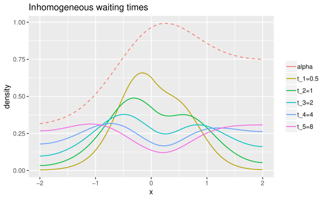
Figure 1: Continuous interface problem. Coefficients are as given in the text, and $c=400$.

Korabel and Barkai (2010) have studied a one-dimensional subdiffusive lattice with exponent $\beta=0.3$ for $x<0$ and $\beta=0.75$ for $x>0$, where at the interface ($x=0$) the waiting time is exponentially distributed. Even if particles are biased to jump to the right at $x=0$ and thus the net drift becomes positive, in the long-time limit all particles end up in the left half.

Here we consider a continuous medium that mimics this setup with the coefficients $(\overline{\nu}(w|x),d(x),a(x,t),b(x))$ chosen as follows:

$$\overline{\nu}(w|x) =\frac{w^{-\alpha(x)}}{\Gamma(1-\alpha(x))}\text{ where }\alpha(x)=0.45e^{-x^{2}}+0.3+0.45/(1+e^{-2x}),$$

$$d(x) \equiv 0,\quad a(x,t)\equiv 1,\quad b(x,t)=0.1*\phi(x|0,0.2)$$

where $\phi(x|\mu,\sigma)$ denotes the probability density of the Gaussian distribution with mean $\mu$ and standard deviation $\sigma$. Note that $\alpha(x,t)$ is chosen so that it approaches $0.3$ for large negative $x$, $0.75$ for large positive x and remains just under $1$ near $x=0$.

Figure 1 shows the evolution of the density $P(y,t)$ with a delta function initial condition. At small times we observe two peaks reflecting the trapping that occurs either side of the interface. For late times, one begins to see the aggregation of all particles towards the left hand side ($x<0$) where trapping is stronger (Savov and Toaldo 2018; Fedotov and Falconer 2012).

Straka (2018) shows that changing time units from $T_{0}=1$ to $T_{0}=2$ results in the the updated diffusivity and drift coefficients

$$a_{\beta(x)}(x,t)=\frac{a(x,t)}{T_{0}^{-\alpha(x)}},\quad b_{\beta(x)}(x,t)=\frac{b(x,t)}{T_{0}^{-\alpha(x)}},$$

leading to spatially inhomogeneous temporal scaling. We confirm this by computing probability densities for the parameter tuple $\left(a_{\alpha(x)}(x,t),b_{\alpha(x)}(x),d(x),\overline{\nu}(w|x)\right)$, at the timestamps multiplied by $T_{0}=2$, and plotting the absolute differences (Figure 2). The absolute values of differences are mostly all below 0.015, and remain stable after 8 units of time, indicating that indeed the same densities are calculated in both cases.

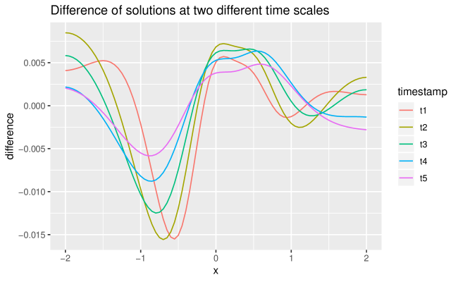
Figure 2: Absolute difference between densities, calculated at corresponding timestamps, for two choices of time scale $T_{0}=1$ and $T_{0}=2$.

5.2 Temporal drift $d(x)$

CTRW limits with positive temporal drift $d(x)$ as per representation (4)–(5) have been studied by Straka (2011): In the case where $Z_{u}$ is a $\beta$ stable Lévy flight, $Z_{u}$ grows superlinearly at the rate $u^{1/\beta}$ both in the short time limit $t\downarrow 0$ and the long time limit $t\uparrow\infty$. Accordingly, the inverse stable subordinator $E(t)$ in (6) grows as $\propto t^{\beta}$, also both in the short time and long time limit. Adding a drift to $Z_{u}$, e.g. $d(x)\equiv d>0$, means that $Z_{u}$ now grows linearly $\propto d\,u$ at short times. Accordingly, its inverse $E(t)$ also grows linearly as $\propto t/d$ at short times. The growth behaviour at late times of $Z_{u}$ and $E(t)$ remains dominated by large jumps resp. long rests, and remains $\propto u^{1/\beta}$ resp. $\propto t^{\beta}$. Hence the addition of the drift $d>0$ means that the slope of $E(t)$ is no longer infinite, and thus the speed of $E(t)$ is tempered at very short times. Figure 3 illustrates the effect of increasing the temporal drift. As can be seen, the jump component of $Z_{u}$ becomes less pronounced as the temporal drift increases, increasing resemblance to a Gaussian process and slowing down the dynamics. Figure 4 shows anomalous diffusion with exponent $0.7$ with spatially varying temporal drift $d(x)$. Particles accumulate in patches of low mobility, corresponding to high $d(x)$.

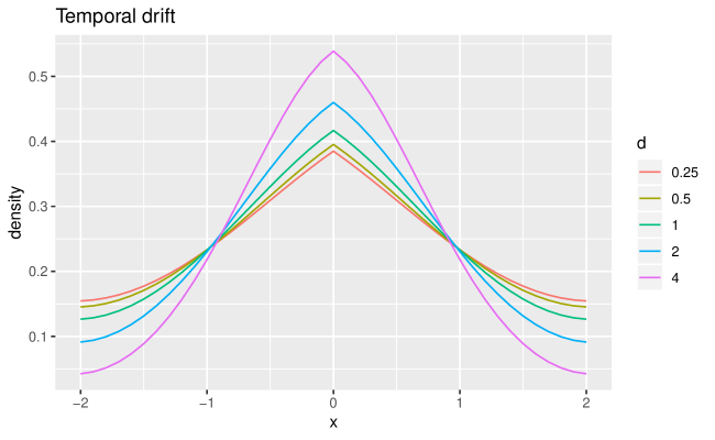
Figure 3: Increasing temporal drift $d(x)$ decreases the speed of the diffusion and increases resemblence to a standard Gaussian process. Parameters: $a(x,t)=0.8,b(x,t)=0,\overline{\nu}(w|x)=w^{-0.7}/\Gamma(1-0.7),c=100,\tau=1/100,\chi=1/10$.

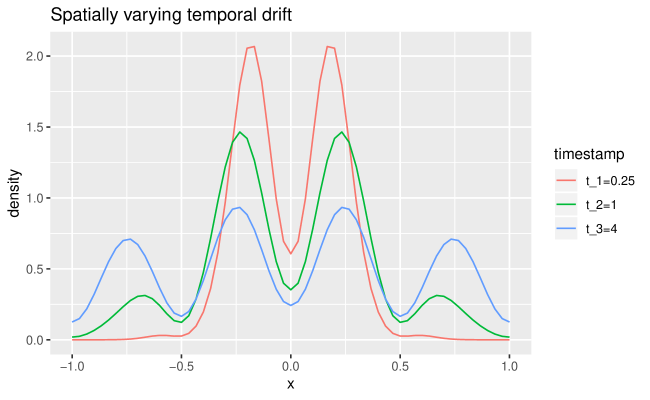
Figure 4: A system with a spatially varying temporal drift $d(x)=10*\sin^{2}(2\pi x)$. Particles accumulate in the slow patches where $d(x)$ is high, while trapping is homogeneous in space. Other parameters: $a(x,t)=0.9$, $b(x,t)=0$, $\overline{\nu}(w|x)=w^{-0.7}/\Gamma(1-0.7)$, $c=900$.

5.3 Variably distributed fractional order

Anomalous diffusion with distributed order assumes a mixing probability distribution of the anomalous parameter $\beta$ with density $p(\beta)$ on the interval $(0,1]$. As illustrated by Sandev et al. (2015), the position of the distributed order fractional operator is decisive for the long-term dynamics. The “natural form” uses the Caputo fractional derivative:

$$\int_{0}^{1}p(\beta)_{C}D_{t}^{\beta}P(y,t)\,d\beta=\frac{1}{2}\frac{\partial^{2}}{\partial y^{2}}P(y,t)$$

Here the mean squared displacement grows proportionally to $t^{\beta_{1}}$ for early times and proportionally to $t^{\beta_{2}}$ for late times, where $\beta_{1}$ is at the left end of the support of $p(\beta)$ and $\beta_{2}$ at the right end. The opposite behaviour occurs for the “modified form”, with Riemann-Liouville fractional derivative:

$$P(y,t)=\int_{0}^{1}p(\beta)_{RL}D_{t}^{1-\beta}\frac{1}{2}\frac{\partial^{2}}{\partial y^{2}}P(y,t)\,d\beta$$

The FFPE for CTRW limits (3) can be rewritten to the natural form, assuming that all coefficients $(a,b,d,\overline{\nu}(w)$ are constant (compare with Eq.(3.8) in Straka 2018 with delta-function initial condition and $\overline{\nu}(t)=t^{-\beta}/\Gamma(1-\beta)$):

$$d\,\frac{\partial}{\partial t}P(y,t)+_{C}D_{t}^{\beta}P(y,t)=\mathcal{L}^{*}P(y,t)$$ (26)

which represents a mixture of the two orders $1$ and $\beta$, with weights $d/(d+1)$ and $1/(d+1)$, after normalization.

We now vary the weights of the two orders in space: Assume a logistic weight $p(y)=1/(1+\exp(-2y)$ with scale $0.5$ for the exponent $1$, and the weight $1-p(y)$ for the exponent $\beta=0.7$. Then the dynamics are diffusive on the far right-hand side, subdiffusive on the far left-hand side, and mixed at the interface near $0$, with continuous interpolation between the two regimes. This is summarized in the coefficient tuple

$$\left(0.9,0,p(y),(1-p(y))w^{-0.7}/\Gamma(1-0.7)\right).$$

Note however that the CTRW limit specified by this tuple is not governed by (26) with weights of $1$ and $\beta$ replaced by $p(y)$ and $1-p(y)$, since the derivation of this equation assumes constant coefficients. We deem it unlikely that a Caputo-type governing equation of the above dynamics exists. The evolution of a system with point mass initial condition at the interface $y=0$ is illustrated in Figure 5.

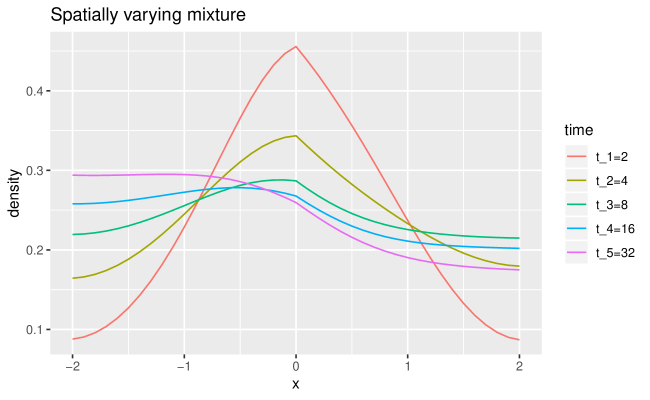
Figure 5: A variable mixture of subdiffusion ($\beta_{1}=0.7$) and diffusion ($\beta_{2}=1$). The two weights add to $1$, and the weight for $\beta_{2}$ equals the logistic function with scale $1/2$, increasing from $0$ on the far left to $1$ on the far right.

5.4 Inverse subordinators

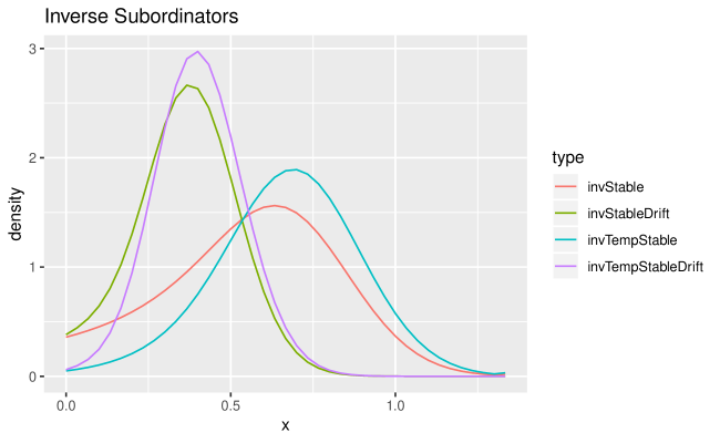
Figure 6: Probability densities for three different types of inverse subordinators, evaluated at time $t=1$, with $c=900$.

The time-changing process $E(t)$ from (6) is well-known in the statistical physics literature as an “inverse subordinator”, and denotes the random crossing time $u$ of a level $t$ by the stable Levy flight $Z_{u}$. Subordination is a widely used method to simulate paths of CTRW limits, see e.g. (Meerschaert and Straka 2013) for an overview. Alrawashdeh et al. (2017) study the “inverse tempered stable subordinator”, i.e. the level crossing time for the tempered stable Levy flight. This process is an important tool for the study of “tempered subdiffusion”, see e.g. Gajda and Magdziarz (2010). Using our algorithm, we may compute probability densities for any inverse subordinator $E(t)$, defined as the level crossing time of any strictly increasing Levy flight.

To this purpose, observe that if $Y_{u}=u$ is linear motion, then we have $X(t)=E(t)$ in (6). In order for $Y_{u}=u$ to hold, we simply let $a(x,t)=0$ and $b(x,t)=1$. In other words, an inverse subordinator is a CTRW limit defined via a coefficient tuple

$$\left(0,1,d,\overline{\nu}(w)\right)$$

A set of jump probabilities which achieves the limits in (14) and (15) is

$$\ell^{(c)}(x,t)=0,\quad n^{(c)}(x,t)=1-\chi,\quad r^{(c)}=\chi.$$

Figure 6 shows probability densities of the inverse stable, inverse tempered stable, inverse stable with drift and inverse tempered stable with drift subordinators. These have coefficient tuples with: $a=0$, $b=1$; in the untempered resp. tempered case, the tail of the Levy measure is

$$\overline{\nu}(w)=\frac{w^{-0.7}}{\Gamma(1-0.7)}\quad\text{ resp.}\quad\overline{\nu}(w)=\frac{w^{-\beta}e^{-\gamma w}-\gamma\Gamma(1-\beta,w)}{\Gamma(1-\beta)}$$

where we set the tempering parameter $\gamma=1$; and for the non-drift resp. drift case, $d=0$ resp. $d=1$. Since tempering makes the Levy flight $Z_{u}$ smaller, $E(t)$ becomes larger. Moreover, a drift $d=1$ introduces the lower bound $u\leq Z_{u}$, which then becomes an upper bound $E(t)\leq t/d$ for the inverse subordinator.

6 Conclusion

We have explored the use of an algorithm which is based on the Semi-Markov property of CTRW limits. To achieve a concise and general representation of CTRW limits, we have identified CTRW limits with a bivariate Langevin process, which in turn is defined via a coefficient tuple $(a(x,t),b(x,t),d(x),\overline{\nu}(w|x))$. Given any such tuple, we can compute probability densities of the CTRW limit at any given time.

The main novel settings to which our algorithm applies are:

• Spatially varying exponents: we have explored two variants of an interface problem, with spatially varying anomalous exponent and spatially varying mixture of two anomalous exponents.

• Temporal drift: a drift added to the Levy flight $Z_{u}$ translates into a “speed limit” for the time evolution $E(t)$, a phenomenon which changes the behaviour at short times of CTRW limits and which is seemingly unknown in the statistical physics literature.

• Inverse subordinators: these are main building blocks for anomalous diffusion problems, and our algorithm computes their densities in great generality.

Contrary to popular knowledge, Semi-Markov processes are not necessarily discontinuous piecewise constant processes with state-dependent holding time distributions. Semi-Markov processes include CTRW limits (with continuous sample trajectories), an idea which we have exploited in this paper. They also include coupled CTRW limits (Straka and Henry 2011) and, in a wider sense, Levy walks (Magdziarz et al. 2015). The main idea from this paper, i.e. leveraging the Semi-Markov property to compute probability densities, can also be applied to these types of processes, which we deem an interesting future extension of the present work.

Acknowledgements

Peter Straka was supported by the Australian Research Council with a Discovery Early Career Researcher Award (DECRA) DE160101147. The authors thank Christopher Angstmann, Bruce Henry and James Nichols for helpful discussions on discrete time random walks.

Reproducibility

All computations and plots of this paper were made using the R programming language (R Core Team 2018) with the rmarkdown (Allaire, Xie, McPherson, et al. 2018) and rticles (Allaire, Xie, R Foundation, et al. 2018) packages. All source code is openly available (Straka and Gill 2018).

Appendix

Appendix A Checking conditions (14) – (17)

The following lemma pertains to the calculations in the waiting times of (14) – (17):

Lemma 1.

Under condition (9), the waiting time distribution (10) satisfies, as $c\to\infty$,

$$\int f(w)\psi^{(c)}(w|y)\,dw=\sum_{j=1}^{\infty}f(j\tau)\psi^{(c)}(j\tau|y) \to f(0),$$ (27)

$$c\int g(w)\psi^{(c)}(w|y)\,dw=c\sum\limits_{j\tau>0}g(j\tau)\psi^{(c)}(j\tau|y) \to\int g(w)\nu(w|y)\,dw,$$ (28)

$$c\int_{0}^{\varepsilon}w\psi^{(c)}(w|y)\,dw=c\sum\limits_{0<j\tau\leq\varepsilon}j\tau\psi^{(c)}(j\tau|y) \to d(y)+\mathcal{O}\left(\frac{\varepsilon^{1-\beta(y)}}{\Gamma(1-\beta(y))}\right),\quad\varepsilon>0.$$ (29)

for any bounded continuous $f$ and $g$, where $g$ vanishes in a neighbourhood of $0$.

Proof. (27) holds since $\psi^{(c)}(w|y)$ is a probability distribution on the positive numbers with tail function

$$\Psi^{(c)}(w|x)=d(x)\mathbf{1}\{w\leq\tau\}+(1-d(x))H^{(c)}(w_{\tau}|x)$$

which for all $w>0$ satisfies $\Psi^{(c)}(w|y)\to 0$ as $c\to\infty$ (recall that $\tau=1/c\downarrow 0$). For (28), we first note that

$$c\Psi^{(c)}(w|y)=cd(y)\mathbf{1}(w\leq\tau)+[c(1-d(y))]\wedge\overline{\nu}(w_{\tau})\to\overline{\nu}(w),\quad c\to\infty,$$ (30)

for every $w>0$. Assume that $g$ is differentiable, and let $\varepsilon>0$ be small enough so that $g(\varepsilon)=0$. Using (Lebesgue-Stieltjes) integration by parts, we may calculate

$$c\int_{0}^{\infty}g(w)\psi^{(c)}(w|y)\,dw=c\int_{\varepsilon}^{\infty}g(w)\psi^{(c)}(w|y)\,dw=c\int_{\varepsilon}^{\infty}g^{\prime}(w)\Psi^{(c)}(w|y)\,dw$$

$$\to\int_{\varepsilon}^{\infty}g^{\prime}(w)\overline{\nu}(w|y)\,dw=\int_{\varepsilon}^{\infty}g(w)\nu(w|y)\,dw=\int_{0}^{\infty}g(w)\nu(w|y)\,dw.$$

But bounded continuous functions can be approximated by differentiable functions with arbitrary accuracy, so (28) follows.

Finally, for (29), we consider the local and nonlocal parts $\psi^{(c)}_{\rm loc}(w|x)$ and $\psi^{(c)}_{\rm nonloc}(w|x)$ separately. For the local part, we have

$$c\int_{0}^{\varepsilon}w\,\psi^{(c)}_{\rm loc}(w|x)\,dw=c\tau\to 1.$$

For the nonlocal part, we use Lebesgue-Stieltjes integration by parts:

$$\int_{0}^{\varepsilon}w\,\psi^{(c)}_{\rm nonloc}(w|x)\,dw=\int_{0}^{\varepsilon}w\,\left(-d\Psi^{(c)}_{\rm nonloc}(w|x)\right)$$

$$=-\left[w\Psi^{(c)}_{\rm nonloc}(w|x)\right]_{0}^{\varepsilon}+\int_{0}^{\varepsilon}\Psi^{(c)}_{\rm nonloc}(w|x)\,dw$$

$$=-\varepsilon\Psi^{(c)}_{\rm nonloc}(\varepsilon|x)+\int_{0}^{\varepsilon}\Psi^{(c)}_{\rm nonloc}(w|x)\,dw$$

Multiplying with $c$ and letting $c\to\infty$, the right hand side converges to

$$-\frac{\varepsilon\overline{\nu}(\varepsilon|x)}{1-d(x)}+\int_{0}^{\varepsilon}\frac{\overline{\nu}(\varepsilon|x)}{1-d(x)}\,dw$$

where both terms are of order $\mathcal{O}\left(\varepsilon^{1-\beta(x)}/\Gamma(1-\beta(x))\right)$ according to the technical assumption (9). (29) now follows from the definition (10) of $\psi^{(c)}(w|x)$. ∎

The final lemma pertains to the jump distributions in (14)–(17):

Lemma 2.

The jump probabilities $\ell^{(c)}(x,t),r^{(c)}(x,t)$ and $n(x,t)$ satisfy

$$c[-\chi\ell^{(c)}(x,t+w)+\chi r^{(c)}(x,t+w)] =b(x,t+w)$$ (31)

$$c\chi^{2}[\ell^{(c)}(x,t+w)+r^{(c)}(x,t+w)] =a(x,t+w)$$ (32)

$$\int_{\mathbb{R}}f(z)\left[r^{(c)}(x,t)\delta_{\chi}(z)+n(x,t)\delta_{0}(z)+\ell^{(c)}(x,t)\delta_{-\chi}(z)\right]\,dz \to f(0)$$ (33)

as $c\to\infty$ for all bounded continuous $f$.

Proof. This follows easily from the definitions of the jump probabilities. ∎

Finally, to see that (14)–(15) hold, use (31)–(32) and (27). To see (16), use (29) and let $\varepsilon\downarrow 0$; and finally, to see (17), use (28) and (33).

References

Allaire, JJ, Yihui Xie, Jonathan McPherson, Javier Luraschi, Kevin Ushey, Aron Atkins, Hadley Wickham, Joe Cheng, and Winston Chang. 2018. Rmarkdown: Dynamic Documents for R. https://CRAN.R-project.org/package=rmarkdown.

Allaire, JJ, Yihui Xie, R Foundation, Hadley Wickham, Journal of Statistical Software, Ramnath Vaidyanathan, Association for Computing Machinery, et al. 2018. Rticles: Article Formats for R Markdown. https://CRAN.R-project.org/package=rticles.

Alrawashdeh, Mahmoud S., James F. Kelly, Mark M Meerschaert, and Hans Peter Scheffler. 2017. “Applications of inverse tempered stable subordinators.” Comput. Math. with Appl. 73 (6). Elsevier Ltd: 892–905. doi:10.1016/j.camwa.2016.07.026.

Angstmann, C.N., I.C. Donnelly, Bruce I Henry, B.A. Jacobs, T.A.M. Langlands, and J.A. Nichols. 2016. “From stochastic processes to numerical methods: A new scheme for solving reaction subdiffusion fractional partial differential equations.” J. Comput. Phys. 307 (February). Elsevier Inc.: 508–34. doi:10.1016/j.jcp.2015.11.053.

Angstmann, Christopher N, Isaac C Donnelly, Bruce I Henry, and James A Nichols. 2015. “A discrete time random walk model for anomalous diffusion.” J. Comput. Phys. 293. Elsevier Inc.: 53–69. doi:10.1016/j.jcp.2014.08.003.

Angstmann, Christopher N, Isaac C Donnelly, Bruce I Henry, T. A. M. Langlands, and Peter Straka. 2015. “Generalized Continuous Time Random Walks, Master Equations, and Fractional Fokker–Planck Equations.” SIAM J. Appl. Math. 75 (4): 1445–68. doi:10.1137/15M1011299.

Applebaum, D. 2009. Lévy Processes and Stochastic Calculus. Book. 2nd ed. Vol. 116. Cambridge Studies in Advanced Mathematics. Cambridge University Press.

Baeumer, Boris, and Peter Straka. 2016. “Fokker–Planck and Kolmogorov Backward Equations for Continuous Time Random Walk scaling limits.” Proc. Am. Math. Soc., 1–14. doi:10.1090/proc/13203.

Banks, Daniel S., and Cécile Fradin. 2005. “Anomalous diffusion of proteins due to molecular crowding.” Biophys. J. 89 (5): 2960–71. doi:10.1529/biophysj.104.051078.

Berkowitz, Brian, Simon Emmanuel, and H. Scher. 2008. “Non-Fickian transport and multiple-rate mass transfer in porous media.” Water Resour. Res. 44 (3): 1–16. doi:10.1029/2007WR005906.

Chen, Chang-Ming, F. Liu, V. Anh, and I. Turner. 2010. “Numerical Schemes with High Spatial Accuracy for a Variable-Order Anomalous Subdiffusion Equation.” SIAM J. Sci. Comput. 32 (4): 1740–60. doi:10.1137/090771715.

Fedotov, Sergei, and Steven Falconer. 2012. “Subdiffusive master equation with space-dependent anomalous exponent and structural instability.” Phys. Rev. E 85 (3): 031132. doi:10.1103/PhysRevE.85.031132.

Gajda, Janusz, and Marcin Magdziarz. 2010. “Fractional Fokker-Planck equation with tempered $\alpha$-stable waiting times: Langevin picture and computer simulation.” Phys. Rev. E 82 (1): 1–6. doi:10.1103/PhysRevE.82.011117.

Gardiner, C.W. 2004. Handbook of Stochastic Methods for Physics, Chemistry, and the Natural Sciences. Springer Complexity. Springer. https://books.google.com.au/books?id=wLm7QgAACAAJ.

Gill, Gurtek, and Peter Straka. 2016. “A Semi-Markov Algorithm for Continuous Time Random Walk Limit Distributions.” Edited by A. Nepomnyashchy and V. Volpert. Math. Model. Nat. Phenom. 11 (3): 34–50. doi:10.1051/mmnp/201611303.

Hahn, Marjorie G, Kei Kobayashi, J. Ryvkina, and Sabir Umarov. 2011. “On time-changed Gaussian processes and their associated Fokker-Planck-Kolmogorov equations.” Electron. Commun. Probab. 16: 150–64. http://www.emis.ams.org/journals/EJP-ECP/_ejpecp/ECP/include/getdocc776.pdf?id=5619&article=2284&mode=pdf.

Hanert, Emmanuel, and Cécile Piret. 2014. “A Chebyshev PseudoSpectral Method to Solve the Space-Time Tempered Fractional Diffusion Equation.” SIAM J. Sci. Comput. 36 (4): A1797–A1812. doi:10.1137/130927292.

Henry, Bruce I, T. A. M. Langlands, and Peter Straka. 2010. “Fractional Fokker-Planck Equations for Subdiffusion with Space- and Time-Dependent Forces.” Journal article. Phys. Rev. Lett. 105 (17). American Physical Society: 170602. doi:10.1103/PhysRevLett.105.170602.

Henry, Bruce I, T. A.M. Langlands, Peter Straka, and T. A. M. Langlands. 2010. “An introduction to fractional diffusion.” Journal article. In Complex Phys. Biophys. Econophysical Syst. World Sci. Lect. Notes Complex Syst., edited by R L. Dewar and F Detering, 9:37–90. World Scientific Lecture Notes in Complex Systems. Singapore: World Scientific. doi:10.1142/9789814277327_0002.

Höfling, Felix, Thomas Franosch, and Review Article. 2012. “Anomalous transport in the crowded world of biological cells,” 1–55.

Korabel, Nickolay, and Eli Barkai. 2010. “Paradoxes of subdiffusive infiltration in disordered systems.” Phys. Rev. Lett. 104 (17): 1–4. doi:10.1103/PhysRevLett.104.170603.

Langlands, T. A. M., and Bruce I Henry. 2005. “The accuracy and stability of an implicit solution method for the fractional diffusion equation.” J. Comput. Phys. 205 (2): 719–36. doi:10.1016/j.jcp.2004.11.025.

Li, Xianjuan, and Chuanju Xu. 2009. “A Space-Time Spectral Method for the Time Fractional Diffusion Equation.” SIAM J. Numer. Anal. 47 (3): 2108–31. doi:10.1137/080718942.

Magdziarz, Marcin, Hans-Peter Scheffler, Peter Straka, and P.d Zebrowski. 2015. “Limit theorems and governing equations for Lévy walks.” Stoch. Process. Their Appl. 125 (11). Elsevier B.V.: 4021–38. doi:10.1016/j.spa.2015.05.014.

Meerschaert, Mark M, and Peter Straka. 2012. “Fractional Dynamics at Multiple Times.” J. Stat. Phys. 149 (5): 878–86. doi:10.1007/s10955-012-0638-z.

———. 2013. “Inverse Stable Subordinators.” Edited by A. Nepomnyashchy and V. Volpert. Math. Model. Nat. Phenom. 8 (2): 1–16. doi:10.1051/mmnp/20138201.

———. 2014. “Semi-Markov approach to continuous time random walk limit processes.” Ann. Probab. 42 (4): 1699–1723. doi:10.1214/13-AOP905.

Metzler, Ralf, and Joseph Klafter. 2000. “The random walk’s guide to anomalous diffusion: a fractional dynamics approach.” Journal article. Phys. Rep. 339 (1). Elsevier: 1–77. doi:10.1016/S0370-1573(00)00070-3.

Mustapha, Kassem, and William McLean. 2011. “Piecewise-linear, discontinuous Galerkin method for a fractional diffusion equation.” Numer. Algorithms 56 (2): 159–84. doi:10.1007/s11075-010-9379-8.

Orsingher, Enzo, Costantino Ricciuti, and Bruno Toaldo. 2018. “On semi-Markov processes and their Kolmogorov’s integro-differential equations.” J. Funct. Anal. 275 (4). Elsevier Inc.: 830–68. doi:10.1016/j.jfa.2018.02.011.

R Core Team. 2018. R: A Language and Environment for Statistical Computing. Vienna, Austria: R Foundation for Statistical Computing. https://www.R-project.org/.

Regner, Benjamin M., Dejan Vučinić, Cristina Domnisoru, Thomas M. Bartol, Martin W. Hetzer, Daniel M. Tartakovsky, and Terrence J. Sejnowski. 2013. “Anomalous diffusion of single particles in cytoplasm.” Biophys. J. 104 (8): 1652–60. doi:10.1016/j.bpj.2013.01.049.

Sandev, Trifce, Aleksei V. Chechkin, Nickolay Korabel, Holger Kantz, Igor M. Sokolov, and Ralf Metzler. 2015. “Distributed-order diffusion equations and multifractality: Models and solutions.” Phys. Rev. E - Stat. Nonlinear, Soft Matter Phys. 92 (4): 1–19. doi:10.1103/PhysRevE.92.042117.

Santamaria, Fidel, Stefan Wils, Erik De Schutter, and George J. Augustine. 2006. “Anomalous diffusion in Purkinje cell dendrites caused by spines.” Neuron 52 (4): 635–48. doi:10.1016/j.neuron.2006.10.025.

Savov, Mladen, and Bruno Toaldo. 2018. “Semi-Markov processes, integro-differential equations and anomalous diffusion-aggregation,” 1–37. http://arxiv.org/abs/1807.07060.

Scalas, Enrico. 2006. “The application of continuous-time random walks in finance and economics.” Phys. A Stat. Mech. Its Appl. 362: 225–39.

Schumer, Rina, David A Benson, Mark M Meerschaert, and Boris Baeumer. 2003. “Fractal mobile/immobile solute transport.” Water Resour. Res. 39 (10). doi:10.1029/2003WR002141.

Sokolov, Igor M, and Joseph Klafter. 2006. “Field-Induced Dispersion in Subdiffusion.” Phys. Rev. Lett. 97 (14): 1–4. doi:10.1103/PhysRevLett.97.140602.

Stickler, B. A., and E. Schachinger. 2011. “Continuous time anomalous diffusion in a composite medium.” Phys. Rev. E - Stat. Nonlinear, Soft Matter Phys. 84 (2): 1–9. doi:10.1103/PhysRevE.84.021116.

Straka, Peter. 2011. “Continuous Time Random Walk Limit Processes: Stochastic Models for Anomalous Diffusion.” PhD thesis, University of New South Wales. http://unsworks.unsw.edu.au/fapi/datastream/unsworks:9800/SOURCE02.

———. 2018. “Variable order fractional Fokker–Planck equations derived from Continuous Time Random Walks.” Physica A: Statistical Mechanics and Its Applications 503 (August): 451–63. doi:10.1016/j.physa.2018.03.010.

Straka, Peter, and Sergei Fedotov. 2015. “Transport equations for subdiffusion with nonlinear particle interaction.” J. Theor. Biol. 366 (February). Elsevier: 71–83. doi:10.1016/j.jtbi.2014.11.012.

Straka, Peter, and Gurtek Gill. 2018. “Strakaps/Varyexp V1.0.” doi:10.5281/zenodo.1346346.

Straka, Peter, and Bruce I Henry. 2011. “Lagging and leading coupled continuous time random walks, renewal times and their joint limits.” Stoch. Process. Their Appl. 121 (2). Elsevier B.V.: 324–36. doi:10.1016/j.spa.2010.10.003.

Tolić-Nørrelykke, Iva Marija, Emilia-Laura Munteanu, Genevieve Thon, Lene Oddershede, and Kirstine Berg-Sørensen. 2004. “Anomalous Diffusion in Living Yeast Cells.” Phys. Rev. Lett. 93 (7): 078102. doi:10.1103/PhysRevLett.93.078102.

Weron, A., and Marcin Magdziarz. 2008. “Modeling of subdiffusion in space-time-dependent force fields beyond the fractional Fokker-Planck equation.” Journal article. Phys. Rev. E 77 (3). APS: 1–6. doi:10.1103/PhysRevE.77.036704.

Whitt, Ward. 2001. Stochastic-Process Limits: An Introduction to Stochastic-Process Limits and their Application to Queues. Book. 1st ed. New York: Springer.

Wong, I Y, M L Gardel, D R Reichman, Eric R Weeks, M T Valentine, A R Bausch, and D A Weitz. 2004. “Anomalous Diffusion Probes Microstructure Dynamics of Entangled F-Actin Networks.” Phys. Rev. Lett. 92 (17): 178101. doi:10.1103/PhysRevLett.92.178101.

Yuste, S B, and L Acedo. 2005. “An Explicit Finite Difference Method and a New von Neumann-Type Stability Analysis for Fractional Diffusion Equations” 42 (5): 1862–74. doi:10.1137/030602666.