Efficient singular-value decomposition of the coupled-cluster triple excitation amplitudes

Abstract

We demonstrate a novel technique to obtain singular-value decomposition (SVD) of the coupled-cluster triple excitations amplitudes, $t_{ijk}^{abc}$. The presented method is based on the Golub-Kahan bidiagonalization strategy and does not require $t_{ijk}^{abc}$ to be stored. The computational cost of the method is comparable to several CCSD iterations. Moreover, the number of singular vectors to be found can be predetermined by the user and only those singular vectors which correspond to the largest singular values are obtained at convergence. We show how the subspace of the most important singular vectors obtained from an approximate triple amplitudes tensor can be used to solve equations of the CC3 method. The new method is tested for a set of small and medium-sized molecular systems in basis sets ranging in quality from double- to quintuple-zeta. It is found that to reach the chemical accuracy ($\approx 1$ kJ/mol) in the total CC3 energies as little as $5-15\%$ of SVD vectors are required. This corresponds to the compression of the $t_{ijk}^{abc}$ amplitudes by a factor of ca. $0.0001-0.005$. Significant savings are obtained also in calculation of interaction energies or rotational barriers, as well as in bond-breaking processes.

Keywords: coupled-cluster theory, singular-value decomposition, electronic structure  

Error in the CC3 correlation energy (in mH) for water molecule (cc-pV5Z basis set) as a function of number of singular vectors ($N_{v}$) included in the expansion of triple excitation amplitudes. The horizontal red dashed line marks the $1$ kJ/mol accuracy threshold (the chemical accuracy).

Introduction

Over the past several decades the coupled cluster (CC) theory ^{1, 2, 3, 4, 5, 6} has established itself as one of the most successful quantum chemical methods (see Ref. 7 for an extended survey). In particular, the CCSD(T) method of Raghavachari et al. ⁸ serves as the gold standard of quantum chemistry ^{9, 10, 11, 12, 13}. In well-behaved systems CCSD(T) is able to consistently deliver results of chemical accuracy (in the complete basis set limit) and thus provide a benchmark for other theoretical models. Some cases when the CCSD(T) method breaks down have also been intensively studied^{14, 15, 16, 17} and various extensions and corrections have been proposed. This includes the so-called externally corrected CC methods ^{18, 19, 20, 21, 22, 23, 24}, renormalized and completely renormalized CC approaches of Piecuch and collaborators ^{25, 26, 27, 28, 29, 30, 31, 32, 33, 34, 35, 36, 17}, the CC(P;Q) hierarchy of techniques introduced recently ^{37, 38, 39, 40, 41, 42}, approaches based on partitioning of a similarity-transformed Hamiltonian ^{43, 44, 45, 46, 47, 48}, the orbital-optimized methods ^{49, 50, 51, 52}, and techniques which incorporate the so-called $\Lambda$ amplitudes ^{53, 54, 55, 56}.

An important observation related to the higher-order clusters ($T_{n}$) in the CC theory is that only a relatively small number of excitations (or linear combinations thereof) contribute significantly to the correlation energy and other results. It is therefore natural to attempt to extract the important information from $T_{n}$, i.e. reduce the rank of a high-rank tensor $T_{n}$, and the singular-value decomposition (SVD) ⁵⁷ is a prominent method for accomplishing such task. It has been successfully used in numerous applications from signal processing ^{58, 59} and data analysis ^{60, 61} to psychometrics ⁶².

In the context of the CC theory the use of SVD has been first considered by Hino at al. ^{63, 64} who have shown how CCSDT-1a equations can be solved in a SVD subspace. However, no efficient methods have been known thus far to compute SVD of a given $t_{ijk}^{abc}$ tensor. In Ref. 64 this was achieved by diagonalization of a certain pseudo-density matrix. Unfortunately, the cost of computation of this matrix scales as $\mathcal{N}^{8}$ with the size of the system, $\mathcal{N}$, which is formally the same (up to a prefactor) as the cost of the complete CCSDT computations. This eliminates all potential gains from the compression of the $T_{3}$ amplitudes. Nonetheless, the results of Ref. 64 are very important as they suggest that the overall idea is sound provided that a more economical method of computing SVD of $t_{ijk}^{abc}$ tensor can be found. The main purpose of this work is to establish such a method.

We have adopted a set of important requirements which must simultaneously be fulfilled for the method to be of any use in quantum chemistry. First, the $T_{3}$ amplitudes need not to be stored in memory; some portion of the $t_{ijk}^{abc}$ tensor can be stored, e.g. after some pre-screening is applied, but this should be an option, not a requirement. Second, the computational cost of the procedure should be smaller than $\mathcal{N}^{8}$, for the reasons explained earlier. Third, the method should be able to selectively find only the most important singular vectors, i.e. those that correspond to the largest singular values, and the desired number of vectors should be set by the user beforehand. Finally, the method should be as close to a black-box as possible and require a minimal user input and intervention.

To test the new method we employ a subspace formed by the most important singular vectors (obtained from SVD of an approximate $T_{3}$ amplitudes) to solve equations of iterative CC methods. It would be natural to apply this idea to the most complete CCSDT model. However, this requires careful consideration of the details of the implementation including factorization of several high-order terms and is beyond the scope of the present work. Instead, we concentrate on the CC3 method ⁶⁵ which is a successful and widely used approximation to the full CCSDT theory.

Theory

Preliminaries

Coupled cluster theory is based on exponential parametrization of the many-electron wavefunction

$$|\Psi\rangle=e^{T}\,|\phi_{0}\rangle,$$ (1)

where $|\phi_{0}\rangle$ is the reference determinant and $T=\sum_{n=1}T_{n}$ are the cluster operators expressed through the creation $a^{\dagger},b^{\dagger},\ldots$, and annihilation operators $i,j,\ldots$ as

$$T_{1}=\sum_{ai}t_{i}^{a}\,a^{\dagger}i,$$ (2)

$$T_{2}=\frac{1}{4}\sum_{abji}t_{ij}^{ab}\,a^{\dagger}b^{\dagger}ji,$$ (3)

$$T_{3}=\frac{1}{36}\sum_{abckji}t_{ijk}^{abc}\,a^{\dagger}b^{\dagger}c^{\dagger}kji,$$ (4)

and so on. The indices $i,j,k,\ldots$ and $a,b,c,\ldots$ denote the occupied and virtual spin-orbitals, respectively. When the occupation of an orbital is not specified we use general indices $p,q,r,\ldots$. Throughout the paper the canonical Hartree-Fock determinant is assumed as the reference wavefunction and the spin-orbital energies are denoted by $\epsilon_{p}$. For further use, we also introduce a shorthand notation $\langle X\rangle\stackrel{{\scriptstyle\mbox{\tiny def}}}{{=}}\langle\phi_{0}|X\phi_{0}\rangle$ and $\langle X|Y\rangle\stackrel{{\scriptstyle\mbox{\tiny def}}}{{=}}\langle X\phi_{0}|Y\phi_{0}\rangle$ for arbitrary operators $X$, $Y$. The electronic Schrödinger Hamiltonian is divided into two parts, $H=F+W$, where $F$ is the Fock operator and $W$ is the fluctuation potential.

The conventional CC equations are obtained by inserting the Ansatz (1) into the electronic Schrödinger equation and projecting onto the manifold of singly, doubly, etc., excited states determinants. The electronic energy is given by the expression $E=\langle e^{-T}He^{T}\rangle$. By truncating the cluster operator at a certain level one obtains approximate CC models. For example, by setting $T=T_{1}+T_{2}$ and projecting onto $\langle\,_{i}^{a}|$, $\langle\,_{ij}^{ab}|$ one recovers the standard CCSD theory ^{66, 67, 68, 69}. An analogous truncation $T=T_{1}+T_{2}+T_{3}$ combined with projection onto $\langle\,_{i}^{a}|$, $\langle\,_{ij}^{ab}|$, $\langle\,_{ijk}^{abc}|$ gives the CCSDT theory ^{70, 71}.

A popular method to reduce the computational burden connected with the inclusion of the $T_{3}$ operator is to invoke a perturbative approach. For example, in the CCSD[T] method ^{72, 73} the amplitudes $T_{3}$ are approximated by the leading-order perturbative expression

$$T_{3}^{[2]}=(\epsilon_{ijk}^{abc})^{-1}\langle\,_{ijk}^{abc}|\big{[}W,T_{2}\big{]}\rangle\,a^{\dagger}b^{\dagger}c^{\dagger}kji,$$ (5)

where $\epsilon_{ijk}^{abc}=\epsilon_{i}+\epsilon_{j}+\epsilon_{k}-\epsilon_{a}-\epsilon_{b}-\epsilon_{c}$ is the three-particle energy denominator. This leads to a relatively simple energy correction which is added on top of CCSD

$$E^{[4]}_{T}=\langle T_{2}|\big{[}W,T_{3}^{[2]}\big{]}\rangle.$$ (6)

Working expressions of the CCSD(T) method are virtually the same apart from one term, $\langle\,T_{1}|\big{[}W,T_{3}^{[2]}\big{]}\rangle$, which involves singly excited configurations ⁸. The computational cost of evaluating $E^{[4]}_{T}$ scales as $\mathcal{N}^{7}$.

A different (non-perturbative) way of simplifying the CCSDT method relies on adopting approximations to the $T_{3}$ amplitudes equations yet retaining the iterative nature of the theory. Several variants such as CCSDT-n, $n=1,2,3$, of Urban et al. ^{74, 75} were proposed but in the present paper we rely on the CC3 method introduced by Koch et al. ⁶⁵ The singles and doubles equations in the CC3 method are exactly the same as in CCSDT but the triples equation is simplified to the form

$$\langle\,_{ijk}^{abc}|\big{[}F,T_{3}\big{]}+\big{[}\widetilde{W},T_{2}\big{]}\rangle=0,$$ (7)

where $\widetilde{W}=e^{-T_{1}}We^{T_{1}}$. The CC3 method scales as $\mathcal{N}^{7}$ which is formally the same as CCSD(T). In practice, CC3 is considerably more expensive than CCSD(T) due to its iterative nature but still orders of magnitude cheaper than the full CCSDT.

For convenience of the readers let us briefly recall the most important properties of the singular-value decomposition. An in-depth discussion of this topic can be found, for example, in Ref. 57. SVD is a factorization of an arbitrary $m\times n$ rectangular matrix ${\bf M}$ to the form

$${\bf M=U\,\Sigma V^{\dagger}},$$ (8)

where the following statements are valid about the matrices $\bf U$, $\bf\Sigma$, and $\bf V$

• ${\bf U}$ is an $m\times m$ unitary matrix collecting orthonormal eigenvectors of ${\bf MM^{\dagger}}$ (left-singular vectors);

• ${\bf V}$ is an $n\times n$ unitary matrix collecting orthonormal eigenvectors of ${\bf M^{\dagger}M}$ (right-singular vectors);

• ${\bf\Sigma}$ is a rectangular $m\times n$ diagonal matrix with non-negative real numbers on the diagonal (singular values).

The singular values are identical to square roots of non-zero eigenvalues of ${\bf MM^{\dagger}}$ (or ${\bf M^{\dagger}M}$). One of the most useful properties of SVD is that the best (in the sense of the square norm) rank-$r$ approximation to a matrix ${\bf M}$ can be obtained by retaining on the diagonal of $\bf\Sigma$ the largest $r$ singular values and neglecting the rest.

Decomposition of the $T_{3}$ amplitudes

Throughout the paper, we treat the triple amplitudes tensor $t_{ijk}^{abc}$ as a three-dimensional tensor with collective indices $ai$, $bj$, and $ck$. Thus, the dimension of a tensor is $OV$, where $O$ is the number of occupied orbitals and $V$ is the number of virtual orbitals. Moreover, the tensor is symmetric with respect to an exchange of all three indices. The ordering of the orbitals $a$, $i$ within the collective index $ai$ is irrelevant as long it is used consistently in all expressions.

Unfortunately, in three dimensions there exists no decomposition which retains all the merits of the two-dimensional SVD like the optimal truncation property. Therefore, many decomposition strategies have been proposed which possess some desirable properties. In the context of quantum chemistry, the canonical product decomposition^{76, 77, 78, 79} or tensor hypercontraction decomposition ^{80, 81, 82, 83, 84} serve as prime examples. However, the decomposition (or compression) of the $T_{3}$ amplitudes tensor employed here relies on the so-called Tucker-3 format ⁸⁵ which in the present case reads

$$t_{ijk}^{abc}\approx\sum_{XYZ}^{N_{v}}t_{XYZ}\,U^{X}_{ai}\,U^{Y}_{bj}\,U^{Z}_{ck},$$ (9)

or equivalently

$$\hat{T}_{3}\approx\sum_{XYZ}^{N_{v}}t_{XYZ}\,\hat{U}^{X}\hat{U}^{Y}\hat{U}^{Z},\;\; \hat{U}^{X}=\sum_{ai}U^{X}_{ai}\,a^{\dagger}i.$$ (10)

One can say that $t_{XYZ}$ is a compressed triple amplitudes tensor in the subspace spanned by all possible combinations of $\hat{U}^{X}$. Let us introduce the compression factor $\rho\in[0,1]$, defined through the relation $N_{v}=\rho OV$, which measures how successful the compression is. Clearly, in the limit $N_{v}\rightarrow OV$ (or $\rho\rightarrow 1$) the decomposition (10) becomes exact. Note that the same decomposition as in Eq. (9) has been employed by Hino at al. ^{63, 64} to solve equations of the CCSDT-1a method.

The advantage of the Tucker format is that it comes with a prescription on how to select the optimal $U^{X}_{ai}$ (see Refs. 86, 87, 88 for an extended discussion). First, one performs “flattening” of the $t_{ijk}^{abc}$ tensor, i.e. rewrites it as a two-dimensional $O^{2}V^{2}\times OV$ matrix, $t_{aibj,ck}$. Next, SVD of the “flattened“ matrix is performed. The right-singular vectors form the desired tensors $U^{X}_{ai}$ whilst the left-singular vectors can be discarded. The optimal truncation is achieved by selecting those tensors $U^{X}_{ai}$ that correspond to the largest singular values of the “flattened“ matrix.

Compressed CC3 method

The main idea of the compressed CC methods is to perform CC iterations with the $T_{3}$ cluster operator given in the form (10). The matrices $U^{X}_{ai}$ required to form the expansion in Eq. (10) are obtained by performing SVD of some approximate $T_{3}$ amplitudes which must be known in advance. They can be obtained by carrying out the CCSD calculations first and evaluating $T_{3}^{[2]}$. This is the choice adopted in this work but many other options are possible, e.g. taking $T_{3}$ from MRCI calculations within some active-orbital space.

A complete algorithm for computing SVD of an arbitrary $t_{ijk}^{abc}$ tensor is presented in Section III. Here we assume that the necessary matrices $U^{X}_{ai}$ are known and discuss an optimal implementation of the compressed CC3 theory. As a by-product of the SVD procedure the matrices $U^{X}_{ai}$ obey the orthonormality condition

$$\sum_{ai}U^{X}_{ai}\,U^{Y}_{ai}=\delta_{XY}.$$ (11)

As argued in Ref. 64 significant simplifications can be achieved if one performs an orthogonal rotation of the matrices $U^{X}_{ai}$ so that the following relation is fulfilled

$$\sum_{ai}U^{X}_{ai}\,U^{Y}_{ai}\,(\epsilon_{i}-\epsilon_{a})=\epsilon_{X}\delta_{XY},$$ (12)

where $\epsilon_{X}$ are some real-valued constants. This rotation preserves the orthonormality condition (11) and is lossless in terms of the information carried by $U^{X}_{ai}$.

In the CC3 theory the $T_{3}$ amplitudes are given by Eq. (7) which can be rewritten to a more explicit form

$$\epsilon_{ijk}^{abc}\,t_{ijk}^{abc}+\langle\,_{ijk}^{abc}|\big{[}\widetilde{W},T_{2}\big{]}\rangle=0.$$ (13)

Upon inserting the compressed form of the amplitudes, Eq. (9), and making use of Eqs. (11) and (12) one arrives at

$$\left(\epsilon_{X}+\epsilon_{Y}+\epsilon_{Z}\right)t_{XYZ}=\sum_{abcijk}U^{X}_{ai}\,U^{Y}_{bj}\,U^{Z}_{ck}\langle\,_{ijk}^{abc}|\big{[}\widetilde{W},T_{2}\big{]}\rangle,$$ (14)

where $\epsilon_{X}$ have been defined through Eq. (12). Explicit expression for the matrix element on the right-hand-side of the above formula is given in Ref. 65. In the closed-shell case it reads

$$\langle\,_{ijk}^{abc}|\big{[}\widetilde{W},T_{2}\big{]}\rangle=P_{ijk}^{abc}\Big{[}\sum_{d}t_{ij}^{ad}(ck\widetilde{|}bd)-\sum_{l}t_{il}^{ab}(ck\widetilde{|}lj)\Big{]},$$ (15)

where $P_{ijk}^{abc}$ is a permutation operator

$$P_{ijk}^{abc}=\left(\,{}_{ijk}^{abc}\right)+\left(\,{}_{ikj}^{acb}\right)+\left(\,{}_{jik}^{bac}\right)+\left(\,{}_{kij}^{cab}\right)+\left(\,{}_{jki}^{bca}\right)+\left(\,{}_{kji}^{cba}\right),$$ (16)

and $(pq\widetilde{|}rs)$ denotes the dressed ($T_{1}$ similarity-transformed) two-electron integrals ⁶⁵. Note that without the compression the computational cost of evaluating Eq. (15) scales as $O^{3}V^{4}$ in the leading-order term. This typically constitutes a bottleneck in the conventional CC3 calculations. In order to evaluate the expression on the right-hand-side of Eq. (14) we define a handful of intermediate quantities

$$I^{X}_{ai}=\sum_{bj}t_{ij}^{ab}\,U^{X}_{bj},$$ (17)

$$J^{X}_{ab}=\sum_{ci}(ab\widetilde{|}ic)\,U^{X}_{ci},$$ (18)

$$K^{X}_{ij}=\sum_{ka}(ij\widetilde{|}ka)\,U^{X}_{ak}.$$ (19)

The computational cost of calculating $I^{X}_{ai}$, $J^{X}_{ab}$, and $K^{X}_{ij}$ tensors scales as $N_{v}O^{2}V^{2}=\rho\,O^{3}V^{3}$, $N_{v}OV^{3}=\rho\,O^{2}V^{4}$, and $N_{v}O^{3}V=\rho\,O^{4}V^{2}$. In practice, their evaluation is implemented as a series of matrix-matrix multiplications using BLAS routines. We have never found this step to be particularly time-consuming, even for large values of $\rho$.

Expressing the right-hand-side of Eq. (14) in terms of the intermediates (17)$-$(19) yields the final relation for the compressed amplitudes $t_{XYZ}$

$$\left(\epsilon_{X}+\epsilon_{Y}+\epsilon_{Z}\right)t_{XYZ}=P_{XYZ}\Big{[}I_{ai}^{X}\,U_{bi}^{Y}\,J_{ba}^{Z}-I_{ai}^{X}\,U_{aj}^{Y}\,K_{ij}^{Z}\Big{]},$$ (20)

where $P_{XYZ}$ is a permutation operator analogous to Eq. (16) but involving a sum over all possible permutations of the indices $X$, $Y$, $Z$. Evaluation of the first term in the square brackets in Eq. (20) limits the efficiency of the algorithm. The second term in Eq. (20) is by a factor of $O/V$ less expensive. For an efficient implementation of Eq. (20) it is critical that the multiplications of the intermediate matrices are performed in two steps, e.g. $I_{ai}^{X}\left(U_{bi}^{Y}\,J_{ba}^{Z}\right)$. In this particular case the first step scales as $\rho^{2}\,O^{3}V^{4}$ whilst the second as $\rho^{3}O^{4}V^{4}$. We found the former step to be the most time-consuming in almost all test calculations reported further in the text. Taking into account that the evaluation of the uncompressed CC3 triple amplitudes, Eq. (13), scales as $O^{3}V^{4}$ in the leading-order term, we can conclude that the compression reduces this effort by a factor of $\rho^{2}$.

It may be disconcerting that the computational cost of the second step in Eq. (20) scales as $\rho^{3}O^{4}V^{4}$. This would be equivalent to $\mathcal{N}^{8}$ if $O$ and $V$ were simultaneously increased, and the value of $\rho$ were kept fixed. However, as shown numerically in the next sections, when $O$ and $V$ are simultaneously doubled, the optimal $\rho$ is approximately halved. As a result, the asymptotic cost of evaluating Eq. (20) under these circumstances is proportional to $\mathcal{N}^{5}$. One can also consider a different scenario where the values of $\rho$ and $O$ are kept fixed and only $V$ is increased. This corresponds to a situation where, e.g. a small basis set is used to determine $\rho$ and then this $\rho$ is subsequently employed in calculations for the same system with larger basis sets. In this case the computational cost of evaluating Eq. (20) scales as $\mathcal{N}^{4}$, formally the same as the most expensive term in CCSD (with $O$ fixed).

With the compressed triple amplitudes calculated from Eq. (20), the remaining task in the CC3 iteration cycle is to compute $T_{3}$ contributions to the $T_{1}$ and $T_{2}$ amplitude equations, see Eqs. (100) and (101) in Ref. 65. In our pilot implementation this is accomplished by reconstructing (on-the-fly) the triples amplitudes tensor by using Eq. (9). Next, it is inserted into Eqs. (100) and (101) in Ref. 65 to give the final result. Despite this approach is not optimal it has never been found to be the limiting factor in the calculations reported in this work.

Efficient SVD of $T_{3}$ amplitudes

Golub-Kahan bidiagonalization

In this section we present an efficient iterative algorithm to find a predefined number of singular vectors of a given $t_{ijk}^{abc}$ amplitudes tensor. We begin by recalling the key expressions of the Golub-Kahan bidiagonalization method ⁸⁹ which forms a backbone of the present SVD algorithm. Any $m\times n$ rectangular matrix $\mathbf{A}$ can be brought into the bidiagonal form

$$\bf A=PBQ^{\dagger},$$ (21)

where $\bf P$ and $\bf Q$ are $m\times m$ and $n\times n$ unitary matrices, and $\bf B$ is a $m\times n$ upper bidiagonal matrix. The proof of this theorem is constructive and based on the following double recursive formulas

$$\alpha_{j}p_{j}={\bf A}q_{j}-\beta_{j-1}p_{j-1},$$ (22)

$$\beta_{j}q_{j+1}={\bf A}^{\dagger}p_{j}-\alpha_{j}q_{j},$$ (23)

where $p_{j}$ and $q_{j}$ are the $j$-th columns of $\bf P$ and $\bf Q$, respectively, and the constants $\alpha_{j}$ and $\beta_{j}$ are chosen so that $p_{j}$ and $q_{j}$ are normalized. It can be shown that the bidiagonal matrix assumes the following form

$${\bf B}=\left[\begin{matrix}\alpha_{1}&\beta_{1}\\ &\alpha_{2}&\beta_{2}&&\\ &&\alpha_{3}&\beta_{3}\\ &&&\ddots&\ddots\\ &&&&\alpha_{n-1}&\beta_{n-1}\\ &&&&&\alpha_{n}\end{matrix}\right]$$ (24)

and can be padded with zeros to match the required rank. There are two major advantages of the Golub-Kahan procedure. First, it is straightforward to calculate SVD of the matrix $\bf B$ and then reconstruct SVD of the full matrix $\bf A$. Indeed, both $\bf BB^{\dagger}$ and $\bf B^{\dagger}B$ are square tridiagonal matrices and several robust techniques are available in the literature to diagonalize a tridiagonal matrix (see Ref. 90 and references therein). Second, the recursive formulas (22) and (23) contain only products of the matrices $\bf A$ and $\bf A^{\dagger}$ with the vectors $q_{j}$ and $p_{j}$, respectively. They can be calculated on-the-fly without explicit storage of the full $\bf A$ matrix. Unfortunately, in order to obtain accurate singular vectors with the help of Eqs. (22) and (23) one would need to perform a complete bidiagonalization. This is both expensive and wasteful since only a small percentage of the dominant singular vectors is typically needed in practice.

Iterative restarted SVD

Assume one wants to find $r$ singular vectors of the matrix ${\bf A}$ which correspond to the largest singular values. One first selects some dimension $k$ of the search space which must be somewhat larger than $r$. In the first step (initiation) $k$ steps of the Golub-Kahan bidiagonalization are performed. In the matrix notation we may write

$${\bf A}{\bf Q}_{k}={\bf P}_{k}{\bf B}_{k},$$ (25)

$${\bf A}^{\dagger}{\bf P}_{k}={\bf Q}_{k}{\bf B}_{k}^{\dagger}+\beta_{k}q_{k+1}e_{k}^{\dagger},$$ (26)

where ${\bf P}_{k}$ and ${\bf Q}_{k}$ are rectangular matrices composed of the first $k$ columns of $\bf P$ and $\bf Q$, respectively, ${\bf B}_{k}$ is the leading $k\times k$ principal sub-matrix of $\bf B$, and $e_{k}$ is a vector of dimension $k$ with unity in the last position. The second term on the right-hand-side of Eq. (26) can be viewed as a remainder which vanishes in the limit of the complete bidiagonalization. In the case of a partial bidiagonalization it allows us to continue the process (restart) by simply employing $q_{k+1}$ in the next step, Eq. (22).

After $k$ steps of the initial bidiagonalization one computes SVD of the ${\bf B}_{k}$ matrix, i.e. , ${\bf B}_{k}={\bf X}_{k}\,{\bf\Sigma}_{k}{\bf Y}_{k}^{\dagger}$. By inserting this formula back into Eqs. (25) and (26) and rearranging we get

$${\bf A}{\bf\bar{Q}}_{k}={\bf\bar{P}}_{k}{\bf\Sigma}_{k},$$ (27)

$${\bf A}^{\dagger}{\bf\bar{P}}_{k}={\bf\bar{Q}}_{k}{\bf\Sigma}_{k}^{\dagger}+\beta_{k}\,q_{k+1}\,e_{k}^{\dagger}{\bf X}_{k},$$ (28)

where ${\bf\bar{Q}}_{k}={\bf Q}_{k}{\bf Y}_{k}$ and ${\bf\bar{P}}_{k}={\bf P}_{k}{\bf X}_{k}$. Now we can select the largest $r$ singular values from ${\bf\Sigma}_{k}$ and shrink the decomposition back to $r$, i.e. temporarily reduce the search space size to $r$ (collapse). This is done by simply sorting the diagonal elements ($\Sigma_{k}$) in the descending order and neglecting all elements $k>r$ together with the corresponding vectors ${\bf\bar{Q}}_{k}$ and ${\bf\bar{P}}_{k}$. The resulting decomposition is given formally by Eqs. (27) and (28), but with $k$ replaced by $r$ in all instances.

The next phase of the procedure consists of performing additional steps of the Golub-Kahan bidiagonalization in order to increase the search size of the space back to $k$ and thus improve the quality of the desired $r$ singular vectors. Unfortunately, the specific form of the remainder has been destroyed in Eq. (28), so that it is no longer proportional to $q_{k+1}\,e_{k}^{\dagger}$ for some vector $q_{k+1}$. As argued earlier, this form must be restored in order to facilitate the search space expansion. For this purpose we adopt the method put forward by Baglama and Reichel ⁹¹. The idea is to expand the search space by one pair of vectors $r\rightarrow r+1$ which are purposefully chosen so that the correct bidiagonal form analogous to Eqs. (25) and (26) is restored. This is accomplished by setting

$${\bf\bar{Q}}_{r+1}=\big{[}\,\bar{q}_{1},\bar{q}_{2},\ldots,\bar{q}_{p},q_{k+1}\big{]},$$ (29)

where $q_{k+1}$ is taken from Eq. (26), and

$${\bf\bar{P}}_{r+1}=\big{[}\,\bar{p}_{1},\bar{p}_{2},\ldots,\bar{p}_{p},\bar{p}_{r+1}\big{]},$$ (30)

where $\bar{p}_{r+1}$ is obtained by normalizing the following vector

$$x=Aq_{r+1}-\sum_{i=1}^{r}\rho_{i}\bar{p}_{i},$$ (31)

where $\rho_{i}$ are numerical constants chosen to make $\bar{p}_{r+1}$ orthogonal to all previous trial vectors, $\bar{p}_{i}$, $i=1,\ldots,r$. This leads us to the following partial decomposition

$${\bf A}{\bf\bar{Q}}_{r+1}={\bf\bar{P}}_{r+1}{\bf B}_{r+1},$$ (32)

$${\bf A}^{\dagger}{\bf\bar{P}}_{r+1}={\bf\bar{Q}}_{r+1}{\bf B}_{r+1}^{\dagger}+\bar{\beta}_{r+1}\,q_{k+2}\,e_{r+1}^{\dagger},$$ (33)

which is suitable for restart. A minor inconvenience connected with the procedure of Ref. 91 is that the matrix ${\bf B}_{r+1}$ is no longer bidiagonal. Indeed, it possesses the following structure

$${\bf B}_{r+1}=\left[\begin{matrix}\sigma_{1}&&&\rho_{1}\\ &\ddots&&\vdots\\ &&\sigma_{r}&\rho_{r}\\ &&&\bar{\alpha}_{r+1}\\ \end{matrix}\right],$$ (34)

where $\bar{\alpha}_{r+1}=||x||$. After restarting the Golub-Kahan bidiagonalization and expanding the search space back to size $k$ we obtain

$${\bf B}_{k}=\left[\begin{matrix}\sigma_{1}&&&\rho_{1}\\ &\ddots&&\vdots\\ &&\sigma_{r}&\rho_{r}\\ &&&\bar{\alpha}_{r+1}&\beta_{r+1}\\ &&&&\ddots&\ddots\\ &&&&&\alpha_{k-1}&\beta_{k-1}\\ &&&&&&\alpha_{k}\\ \end{matrix}\right].$$ (35)

One can see that the above matrix has a ”spike“ composed of the constants $\rho_{i}$ which prevents it from achieving a proper bidiagonal form. This appears somewhat sub-optimal because one has to use general SVD algorithms to decompose ${\bf B}_{k}$ which are typically less effective than dedicated procedures designed with bidiagonal matrices in mind. In practice, however, the matrix ${\bf B}_{k}$ is rather small and we have never found this step to be particularly troublesome.

To summarize, the iterative restarted SVD procedure described here consists of three phases. In the first phase (initiation) one performs $k$ steps of the ordinary Golub-Kahan bidiagonalization achieving the decomposition given by Eqs. (25) and (26). In the second phase (collapse) one computes SVD of the small matrix ${\bf B}_{k}$. This yields approximate singular values and vectors which are then sorted, and only the most significant vectors are retained in the search space reducing its size to $r$. In the third phase (expansion) of the procedure a pair of vectors is added to the search space, enabling to restart the Golub-Kahan procedure, see Eqs. (27)$-$(34). Finally, the size of the search space is increased to $k$ by performing a certain number of bidiagonalization steps. This allows to return to phase two and establishes an iterative procedure which is repeated until the desired number of singular values/vectors have converged to the prescribed tolerance.

Implementation and technical details

Thus far we have not touched upon a very important aspect of the presented algorithm - selection of the initial vector $q_{0}$ for the bidiagonalization (guess). In principle, any non-zero vector can be used to initiate this process, see Eqs. (22) and (23). However, if the starting vector is unsuitably chosen the algorithm tends to give $\beta_{k}=0$ in Eq. (23) after some number of iterations. This prevents the bidiagonalization process from progressing in the standard fashion and a new vector must be provided in order to continue. We have implemented and tested several possible sources of the starting vectors:

• $T_{1}$ amplitudes;

• successive eigenvectors of the $T_{2}$ amplitudes tensor;

• random vector - elements are generated quasi-randomly on the interval $[-\alpha t_{ai},+\alpha t_{ai}]$, where $t_{ai}$ are the respective elements of the single amplitudes tensor, and $\alpha$ is a positive constant.

The first guess is probably the most efficient in terms of number of iterations but has a considerable disadvantage - once $\beta_{k}=0$ is encountered at some step of the bidiagonalization there is no natural way to continue the process. The $T_{2}$ guess performs only marginally poorer but offers a straightforward way to restart after $\beta_{k}=0$ - one simply selects the next eigenvector in the order of increasing eigenvalues. The random vector guess is a reasonable choice and has the advantage of being cheap and having an infinite supply of vectors for restart. Unfortunately, it also typically requires a larger number of iteration cycles to converge to a good accuracy. To sum up, we found that the guess based on the eigenvectors of the $T_{2}$ amplitudes tensor is the best overall and the overhead connected with the diagonalization is manageable.

Another technical problem related to the bidiagonalization process, Eqs. (22) and (23), is the loss of orthogonality amongst the vectors $p_{j}$ and/or $q_{j}$. This occurs solely due to finite precision of the arithmetic. The simplest remedy to this problem is to perform full orthogonalization at each step, i.e. the new vectors $p_{n}$ and $q_{n}$ are orthogonalized to all previous vectors $p_{i}$ and $q_{i}$, $i=1,\ldots,n-1$, respectively, by using the Gram-Schmidt procedure. The main drawback of this procedure is its high cost which grows as the iterations proceed (note that the size of the vectors $p_{n}$ is $O^{2}V^{2}$). A less expensive alternative to full orthogonalization has been proposed by Simon and Zha ⁹² who observed that loss of orthogonality is mitigated to a sufficient extent when orthogonalization is performed only among $q_{n}$. This one-sided orthogonalization variant has been adopted in all calculations reported in this work.

Finally, let us analyze the computational costs and storage requirements of the presented algorithm. A single step of the Golub-Kahan bidiagonalization requires to multiply the matrix ${\bf A}$ separately from the left and from the right by some trial vectors. In the case of the tensor $t_{ijk}^{abc}=t_{aibj,ck}$ the computational cost of this operation asymptotically scales as $2\cdot O^{3}V^{3}$. The initiation phase of the described algorithm requires to perform $k$ bidiagonalization steps and costs $2k\cdot O^{3}V^{3}$. To estimate the remaining workload let us assume that after $n_{\mbox{\scriptsize it}}$ expansion-collapse cycles the desired $p$ singular vectors have converged to the desired precision. Each cycle consists of expanding the search space from $p+1$ to $k$ and thus requires $k-p-1$ bidiagonalization steps. Therefore, the total cost of the procedure is $2k\cdot O^{3}V^{3}+2n_{\mbox{\scriptsize it}}(k-p-1)\cdot O^{3}V^{3}$. In other words, if the search space size $k$ is equal to the dimension of the flattened matrix, $OV$, the procedure described above is equivalent to the approach adopted by Hino et al. and would possess $\mathcal{N}^{8}$ scaling of the computational costs.

The cost analysis from the previous paragraph assumes that the tensor $t_{ijk}^{abc}$ is stored. In our implementation only non-negligible elements of $t_{ijk}^{abc}$ are stored on the disk in a format which allows to read one row/column at the time. We have also developed a fully direct version of the algorithm where the elements of $t_{ijk}^{abc}$ are calculated on-the-fly as needed. The cost of the on-the-fly algorithm are obviously larger - the overhead depends strongly on the system size and on the efficiency of the prescreening, but it typically amounts to a factor of $5-10$.

One can see that the performance of the algorithm depends on a careful choice of $n_{\mbox{\scriptsize it}}$ and $k$ for a given $p$. In fact, larger $k$ typically require a smaller value of $n_{\mbox{\scriptsize it}}$, but increases the cost of the initiation phase. We found that the optimal choice of the search space size is $k\approx p+10-20$. The only exception from this rule occurs where a large number of vectors is requested (half of the SVD total space size or more). In such cases the value of $k$ must be increased somewhat.

The theory presented here, along with the uncompressed CC3 method, was implemented in a locally modified version of the Gamess program package ⁹³. The validity of the new implementation was verified by comparing with independent routines available in the Psi4 program package ⁹⁴. On-the-fly and semi-direct variants of the Golub-Kahan bidiagonalization scheme, as described earlier in the text, are available. The current version of the code is fine-tuned for decomposition of the $T_{3}^{[2]}$ amplitudes, see Eq. (5), but it can easily be adapted for other sources of an approximate $t_{ijk}^{abc}$ tensor. The present implementation is restricted to closed-shell systems.

Numerical examples

Total correlation energies

In order to investigate the performance of the compressed CC3 method for computation of the correlation energies we performed calculations for 15 small and medium-sized molecules composed of the first- and second-row atoms. The geometries of the molecules considered here were taken from the G2$-$1 and G2$-$2 neutral test sets of Curtiss et al. ⁹⁵ available on the World Wide Web ⁹⁶. For all diatomic and three-atomic molecules we used Dunning-type cc-pV$X$Z basis sets ^{97, 98} ranging in quality from $X=2$ to $X=5$. For larger molecules cc-pV$X$Z basis sets up to $X=4$ were employed. In all calculations reported here the threshold for convergence of the SVD vectors was $10^{-6}$ (in the square norm) and the size of the search space was fixed as $N_{v}+10$, where $N_{v}$ is the desired number of vectors to be found. Under these conditions the convergence of the iteration procedure was typically achieved in under 20 iterations and in many cases only $3-5$ cycles were sufficient. Spherical representation of the Gaussian basis set is employed in all calculations reported here.

For each molecule in the test set we performed SVD-CC3 calculations with varying SVD subspace space, $N_{v}$ in Eq. (9). The value of $N_{v}$ was systematically increased (in steps of $10$) and the error in the correlation energy with respect to the exact CC3 result was recorded. In Table 1 we show the compression levels $\rho$ and the number of SVD vectors which allow to reach the chemical accuracy ($1\,\mbox{kJ/mol}\approx 0.4\,\mbox{mH}$) of the total correlation energy.

Since the maximum possible size of the SVD subspace ($O\cdot V$) is different for each basis set/molecule the quantity $N_{v}$ is not transferable between systems. However, we claim that for a fixed basis set the value of $\rho$ should be (to some extent) transferable between systems of a similar size and thus can be used to estimate how many SVD vectors must be included to meet the adopted accuracy criteria. To confirm this the mean value of $\rho$ for each basis set and the corresponding standard deviation are reported in Table 1. One can see that $\rho=15\%$ is sufficient to reach the chemical accuracy in all systems under consideration and $\rho=10\%$ is adequate for a majority of them. According to the analysis undertaken in the previous section $\rho=15\%$ allows to compress the $T_{3}$ amplitudes tensor by a factor of $\approx 0.003$ and reduce the cost of evaluating Eq. (13) by a factor of $\approx 0.02$.

As presented in Table 1 the average value of $\rho$ decreases significantly when passing from cc-pVDZ to cc-pVTZ. For larger basis sets the average $\rho$ is fairly constant. This observation is of practical interest as it allows to estimate the optimal $\rho$ for a given system from calculations in a small basis set. Moreover, it suggests that SVD-CC methods are expected to be equally useful in calculations with small and large basis sets as the efficiency of the compression is not significantly affected by changing the $V/O$ ratio.

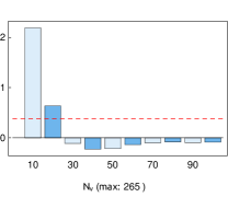
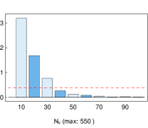
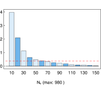
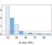
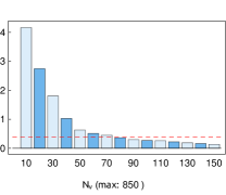
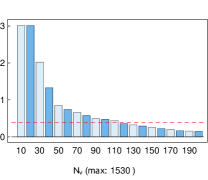
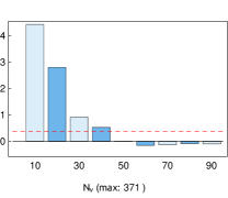
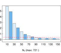
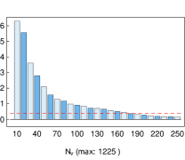
Figure 1: Errors in the SVD-CC3 correlation energies (in mH) as a function of the SVD subspace size ($N_{v}$) with respect to the exact (uncompressed) CC3 method. The results are given for the molecules: water (first row), methane (second row), and carbon monoxide (third row) calculated by using the basis sets cc-pVTZ (first column), cc-pVQZ (second column), and cc-pV5Z (third column). The horizontal red dashed line marks the $1$ kJ/mol accuracy threshold (the chemical accuracy). The maximum possible size of the SVD space is given below each graph.

Another important property of the SVD-CC3 method is the convergence pattern of the correlation energies to the exact results as a function of $N_{v}$. A regular and smooth convergence pattern is a highly desirable property as it allows to verify that the results are saturated with respect to $N_{v}$ and even estimate the error of the calculations. To address this issue we plot the error in the SVD-CC3 correlation energy as a function of $N_{v}$, see Fig. 1. We have selected three test systems: water, methane, and carbon monoxide which represent the best, an average, and the worst performance of the SVD-CC3 method in terms of the value of $\rho$ required to reach the chemical accuracy (based on Table 1). In general, the decay of the error is very regular and, in most cases, the convergence rate is close to exponential. This allows to reach the desired limit in a controllable fashion. The only exception from this rule are the results in small basis sets as illustrated on the left panel of Fig. 1. One can see that in small basis sets the SVD-CC3 method has a tendency to overshoot the correlation energy and then converge to the exact result from below. However, this behavior is not very troublesome as the scale of the overshooting is relatively minor — around $0.1-0.2$ kJ/mol. Moreover, it is not observed in larger basis sets.

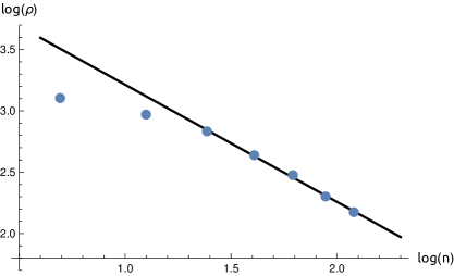
Figure 2: The logarithm of the optimal value of $\rho$ (blue dots) for the chains of equidistant beryllium atoms, $(\mbox{Be})_{n}$, $n=2,3,\ldots,8$, as a function of the logarithm of the chain length, $n$. The black solid line is the least-squares linear fit to the data points $n=4,\ldots,8$.

While the results discussed above prove that the optimal value of $\rho$ is transferable between systems of a similar size, the applicability of SVD-CC methods to larger molecules strongly depends on the asymptotic behavior of $\rho$ for large $\mathcal{N}$. To investigate this issue we performed calculations for linear chains of equidistant beryllium atoms, $(\mbox{Be})_{n}$ with $n=2,3,\ldots,8$, employing the cc-pVDZ basis set. For each $n$ the optimal value of $\rho$ sufficient to reach a constant accuracy of $\approx 1\,$kj/mol per atom was recorded. The distance between the atoms was set to $2.45\,$Å — approximately equal to the equilibrium bond length in $\mbox{Be}_{2}$ molecule ^{99, 100}. Let us assume that the optimal $\rho$ behaves asymptotically as $\mathcal{N}^{-\alpha}$, where $\alpha$ is a parameter independent of $\mathcal{N}$. In other words, on a log-log scale the plot of $\rho$ as a function of $\mathcal{N}$ (and thus the chain length, $n$, since $N\propto n$) should be a straight line. In Fig. 2 we plot $\log\rho$ against $\log n$ for $(\mbox{Be})_{n}$ with $n=2,3,\ldots,8$, together with the corresponding least-squares fit (the outliers $n=2,3$ were eliminated from the fitting procedure). The accuracy of the fit is surprisingly good as measured by the coefficient of determination, $R^{2}=0.998$. From the fit we also empirically determine the value of the parameter $\alpha\approx 0.96$. This proves that the optimal value of $\rho$ decreases with the system size according to an inverse power law. The fact that $\alpha$ determined in this way is so close to the unity also suggests that asymptotically $\rho$ may be simply inversely proportional to $\mathcal{N}$.

In Table 2 we present exemplary timings obtained with our pilot implementation in the Gamess package for methanol molecule in the cc-pVXZ basis sets, X=D,T,Q. We present total timings of the SVD-CC3 calculations that can be compared directly with the uncompressed CC3, but also break down total timings into the most important components (CCSD iterations, Golub-Kahan bidiagonalization etc.). Three typical values of the compression factor, $\rho=5,\,10,\,15\%$, are considered. To allow for a fair comparison all of the aforementioned calculations were performed in the same computational environment (single-core AMD Opteron™Processor 6174) without parallel execution. Moreover, the convergence thresholds and other parameters were kept fixed, and the DIIS convergence accelerator¹⁰¹ was turned off. The timings given in Table 2 show that for cc-pVTZ and cc-pVQZ basis sets some savings with respect to the uncompressed CC3 can be obtained provided that $\rho<10\%$. More importantly, however, one can see that the cost of Golub-Kahan bidiagonalization is comparable to the cost of CCSD iterations. Note that the time spent on diagonalization of the $T_{2}$ amplitudes was not given in Table 2. This is because the cost of this procedure is not significant compared to the other steps of the Golub-Kahan bidiagonalization - for example, in the cc-pVQZ basis set the diagonalization of the $T_{2}$ amplitudes takes only about 3 minutes.

Relative energies

While the results shown in the previous section prove that the compressed CC3 method performs very well in recovering total correlation energies of molecular systems, the energy differences are of principal interest in most applications. Many quantum chemistry methods benefit from a systematic cancellation of errors in evaluation of energy differences. This leads to a significant improvement in their capabilities and thus it is important to determine whether the compressed CC methods also benefit from this phenomenon. To this end, we performed SVD-CC3 calculation of the interaction energies of several molecular complexes and compared the results with the uncompressed CC3 method. The test examples include two hydrogen-bonded complexes (H₂O dimer, HF dimer), a system bound by dispersion forces (CH${}_{4}-$BH₃) and a molecular complex of a mixed induction-dispersion character (CH${}_{4}-$HF). A rather diverse set of model systems were selected to avoid bias towards any particular type of interaction. The geometries were taken from the A24 test set of Řezác̆ and Hobza ¹². The aug-cc-pVTZ basis set ¹⁰² was used in all calculations presented in this section.

Interaction energies calculated for the aforementioned systems are given in Table 3. We list the data starting with $N_{v}=20$ because smaller SVD spaces typically give results which are by an order of magnitude wrong and thus of little practical use. Results given in Table 3 lead to two important conclusions. First, there is a systematic error cancellation in evaluating the energy differences with compressed CC methods. For example, the error of the SVD-CC3 interaction energy for the HF dimer stabilizes below 1 kJ/mol at the compression levels of around $\rho=5\%$. To reach the same level of accuracy in total energies of the HF dimer and of the separated monomers one needs $\rho=10.2\%$ and $\rho=10.9\%$, respectively. Therefore, a significant fraction of the error in raw energies canceled out in evaluation of $E_{\mbox{\scriptsize int}}$. This allows for reliable estimation of the interaction energies with compression factors as small as $5\%$.

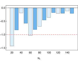
Figure 3: Errors in the interaction energy of the HF dimer (in kJ/mol) calculated with the SVD-CC3 method as a function of the SVD subspace size ($N_{v}$). The horizontal red dashed line marks the $1$ kJ/mol accuracy threshold (the chemical accuracy). The maximum possible size of the SVD space is 1280.

The second conclusion from Table 3 is that the convergence of the SVD-CC3 results towards the exact value as a function of $N_{v}$ is not a smooth as in the case of total energies discussed in the previous section. This is illustrated in Fig. 3 for the HF dimer. While the general convergence pattern is still clear, some accidental cancellations cause the error for several $N_{v}$ to be significantly smaller than the overall trend in the data would suggest. Additionally, the results given in Table 3 suggest that the natural noise level of the SVD-CC3 method is $0.1-0.2$ kJ/mol in the current implementation. This is to be expected due to, e.g. rather loose values of some thresholds set in our program. Nonetheless, this noise level is significantly below the accuracy of the uncompressed CC3 method itself.

As the second illustration of the cancellation of errors in the SVD-CC3 method we consider energy differences between different geometries of the same molecule. The internal rotation of the hydrogen atom around the C$-$O bond in the formic acid is used as a model system. The formic acid has two stable conformers (trans and cis) characterized by H$-$C$-$O$-$H dihedral angle of $0^{\mbox{\scriptsize o}}$ and $180^{\mbox{\scriptsize o}}$, respectively. We calculated energy differences between the trans and cis conformers, height and location of the corresponding rotational barrier. This is achieved by performing potential energy scan varying the H$-$C$-$O$-$H dihedral angle in steps of $15^{\mbox{\scriptsize o}}$ and keeping the remaining internal coordinates of the molecule fixed. The results obtained with SVD-CC3 method are shown in Table 4 and compared with the uncompressed CC3 method. Even with the compression factor as small as $\rho\approx 1\%$ the SVD-CC3 results are wrong only by about $1-2$ kJ/mol. For all intents and purposes the values obtained with $\rho\approx 4\%$ are essentially indistinguishable from the uncompressed CC3 results. This suggest that the cancellation of errors between different geometries of the same molecule is even more substantial than in the calculation of interaction energies. We expect the same conclusion to be valid also in other processes which do not involve breaking of chemical bonds and other drastic rearrangements of electronic densities.

Bond-breaking processes

Let us point out that for a majority of molecules which have been considered thus far in the paper the CCSD(T) method gives acceptable results. In other words, $T_{3}^{[2]}$ is a good approximation to the exact $T_{3}$ cluster operator for these systems and it is reasonable to use it as a source of amplitudes for SVD. However, one can argue that the performance of the SVD-CC methods will be much worse outside the regime of applicability of the $T_{3}^{[2]}$ approximation, e.g. in cases where the CCSD(T) method fails due to significant static correlation effects. Fortunately, the results given in Ref. 64 suggest that this is not true and in this section we provide an additional verification of this claim.

One prominent example of a process where the CCSD(T) method fails both quantitatively and qualitatively is breaking of a chemical bond ^{14, 15, 16, 17}. It is known that CCSD(T) gives nonphysical results even for a relatively simple cleavage of a single bond. To investigate the performance of the SVD-CC3 method in description of this process we performed calculations for bond-breaking reactions in two molecules (F₂ and CH₄). We stretched the F$-$F bond and one of the C$-$H bonds from $0.75\cdot R_{e}$ to $3.00\cdot R_{e}$, where $R_{e}$ is the equilibrium bond length, and calculated the total energies of the system with the following methods:

• conventional CCSD and CCSD(T);

• uncompressed CC3;

• completely renormalized CR-CCSD(T), CR-CC(2,3) methods of Piecuch et al. ¹⁰³;

• SVD-CC3 method with $\rho\approx 5,10,\ldots,25\%$;

• full CCSDT method.

The last method gives negligible errors with respect to FCI for both systems and thus can be used as a reference. The aug-cc-pVTZ basis set is employed in all calculations reported in this section; this is the largest basis set we could use with the CCSDT method. The reference calculations were performed with the AcesII program package ¹⁰⁴.

The results of the calculations are given in Table 5 for the F₂ molecule and in Table 6 for the CH₄ molecule. The first observation is that the standard CCSD(T) method behaves unexpectedly well near the bottom of the potential energy curve. The errors of CCSD(T) for $R=R_{e}$ are one of the smallest among the considered methods, but the accuracy of CCSD(T) deteriorates rapidly when the bond is stretched. As quickly as for $1.25\cdot R_{e}$ SVD-CC3 outperforms CCSD(T). Moreover, for $R>2.0\cdot R_{e}$ the error of CCSD(T) becomes catastrophic while SVD-CC3 retains a fairly constant level of accuracy. Additionally, the SVD-CC3 method with $\rho\approx 10,\,15\%$ offers a considerable improvement over CR-CCSD(T) for nearly all internuclear distances. This behavior is somewhat more pronounced for the F₂ molecule than for CH₄. The performance of CR-CC(2,3) and SVD-CC3 is quite similar – both methods give nearly equivalent results for CH₄, but SVD-CC3 performs somewhat better for F₂. Note that somewhat larger $\rho$ are required here to maintain a satisfactory level of accuracy compared with some of the previous examples given in the paper. However, the $\rho\approx 15\%$ is sufficient for most purposes and the results with $\rho\approx 20\%$ differ insignificantly from the uncompressed CC3 values. To sum up, SVD-CC3 method is able to describe the single-bond breaking process with a consistent accuracy of a few kJ/mol, offering a dramatic improvement over perturbative methods such as CCSD(T) and CR-CCSD(T), and without sacrificing much accuracy for molecules in near-equilibrium geometry.

We have to mention that the comparison between the CR-CCSD(T) (and related methods) and SVD-CC3 is not entirely fair because the latter method is iterative and thus inherently more expensive. In the best case scenario, SVD-CC3 is expected to be twice as expensive as CR-CCSD(T). In practice, we found this ratio to be about 3$-$4 with the compression rates considered here. This overhead is substantial but still acceptable. By comparison, CCSDT computations are hundreds of times more expensive. We could not compare the SVD-CC3 results with $\Lambda$CCSD(T) methods ⁵³ as it is not implemented in any quantum chemistry program available to us.

The results provided in this section show that $T_{3}^{[2]}$ can be used as an initial source of approximate triple excitation amplitudes for SVD even in a non-perturbative regime. It appears that the perturbative expressions manage to correctly identify the important excitations and their rough relative importance but they overestimate the overall effect of the triple excitations. Fortunately, this does not prevent the SVD procedure from extracting the most important information about the exact $T_{3}$ amplitudes.

Summary and conclusions

In this work we have presented a novel method for calculating SVD of the CC triple excitation amplitudes tensor. Our technique is based on the Golub-Kahan bidiagonalization and does not require $T_{3}$ to be stored. Moreover, the cost of the procedure is relatively small - comparable to several CCSD iterations. We have illustrated the usefulness of the new method by computing SVD of an approximate (perturbative) triple excitations amplitudes tensor, and subsequently using the most significant singular vectors as a basis for expansion of the $T_{3}$ cluster operator in the iterative CC3 method.

The resulting SVD-CC3 method has been tested by calculating total correlation energies for a set of small and medium-sized molecules and comparing the results with the exact (uncompressed) CC3 method. We have shown that the compression factors in the range $\rho=5-15\%$ are sufficient to reach the chemical accuracy ($\approx 1$ kJ/mol) of the results. Moreover, we have shown that SVD-CC3 method benefits from a substantial error cancellation in evaluation of, e.g. interaction energies or energy differences between various geometries of the same molecule. It has been found that the compression factors of about $\rho\approx 5\%$ are practically sufficient in evaluation of relative energies.

Finally, we have investigated the performance of the SVD-CC3 method in the processes of breaking of a single bond. The results indicate that SVD-CC3 is free of instabilities found in CCSD(T) and other perturbative methods, and is able to describe single bond-breaking with an accuracy of a few kJ/mol. Let us also point out that SVD-CC3 is a black-box method in the sense that only one input parameter ($\rho$) must be supplied by the user. The remaining internal thresholds and parameters have been kept constant during all calculations reported in this work and no significant technical difficulties have been observed. In particular, there is no need to specify any active orbital space which is both tedious and requires a considerable physical insight into the system being studied.

Since SVD of an approximate triple excitation amplitudes tensor can now be obtained relatively cheaply, i.e. with a cost much lower than $\mathcal{N}^{8}$, the idea of the full SVD-CCSDT method becomes viable. This requires careful factorization of all terms in the CC triples residual, and possibly application of additional decomposition schemes for the $t_{XYZ}$ tensor. However, one can expect the compressed SVD-CCSDT to possess an accuracy level comparable to the full CCSDT, but at a significantly reduced cost. This would provide a relatively inexpensive computational method capable of handling single bond-breaking, biradical species, etc., maintaining the chemical accuracy and the black-box character of single-reference CC methods. To be able to describe double bond-breaking reliably one requires also quadruple excitations to be included in the theoretical model. To this end, various perturbative quadruple corrections ^{105, 72, 106, 107} calculated on top of SVD-CCSDT seem attractive, extending capabilities of the SVD-CC family of methods even further.

Finally, let us point out that in the present work we have avoided using any approximations to the CC equations other than the SVD itself. However, it has been shown that techniques such as density fitting ^{108, 109, 110, 111, 112} or Cholesky decomposition ^{113, 114, 115, 116} are able to reduce the storage and computational requirements of the CC methods without a significant loss in the accuracy ¹¹⁷. Therefore, it would be reasonable to incorporate this techniques in future SVD-CC implementations along with an efficient parallelization. ¹¹⁸

Acknowledgements

I would like to thank Prof. G. Chałasiński and Prof. B. Jeziorski for reading and commenting on the manuscript, and Dr. T. Korona for fruitful discussions concerning the efficiency of coupled-cluster programs. The author is indebted to Prof. P. Piecuch for finding a numerical error in an early version of the manuscript, and to J. Emiliano Deustua, I. Magoulas, and S. H. Yuwono for sharing results of their coupled-cluster calculations which helped to eliminate the problem. This work was supported by the National Science Center, Poland within the project 2017/27/B/ST4/02739.

Table 1: Results of the SVD-CC3 calculations of the total correlation energy. For each basis set the size of the SVD subspace ($N_{v}$) and the corresponding compression factor ($\rho$) are reported which are sufficient to reach the chemical accuracy of the results ($1\,\mbox{kJ/mol}\approx 0.4\,\mbox{mH}$). The values of $\rho$ are given in percents.

	cc-pVDZ		cc-pVTZ		cc-pVQZ		cc-pV5Z
	$N_{v}$	$\rho$	$N_{v}$	$\rho$	$N_{v}$	$\rho$	$N_{v}$	$\rho$
H2O	13	13.0	23	8.5	37	6.7	63	6.4
HCN	13	7.1	47	9.9	97	10.4	188	11.7
CH4	24	16.2	40	9.8	78	9.2	117	7.6
H2CO	32	13.4	61	9.5	151	11.7	—	—
C2H4	43	13.2	115	13.3	219	12.3	—	—
NH3	18	14.9	29	8.7	54	7.7	97	7.7
H2S	34	15.8	52	9.9	66	6.4	210	11.6
C2H2	18	8.2	45	7.9	106	9.3	—	—
CO	19	13.0	43	11.6	88	12.2	178	14.5
CH3OH	47	13.2	83	8.5	200	10.0	—	—
N2H4	49	13.7	78	8.1	240	12.1	—	—
H2O2	36	13.6	62	8.6	179	12.4	—	—
BF3	61	9.4	82	4.9	232	7.1	—	—
NCCN	59	10.6	181	13.0	299	11.1	—	—
LiF	17	12.7	29	8.9	41	6.5	54	5.1
average	—	12.5	—	9.4	—	9.7	—	9.2
std. dev.	—	2.6	—	2.1	—	2.3	—	3.4

Table 2: Single-core timings of the SVD-CC3 method for the methanol molecule in the cc-pVXZ basis sets, X=D,T,Q. The values ”total SVD-CC3“ include timings for all steps of the SVD-CC3 calculations described in the text (CCSD, Golub-Kahan etc.) and can be directly compared with the uncompressed CC3 method (the last row).

task	timings (min)
	cc-pVDZ	cc-pVTZ	cc-pVQZ
Hartree-Fock	0.0	0.7	13.3
four-index trans. (without VVVV)	0.1	0.7	10.9
CCSD (no DIIS)	1.4	30.0	600.0
Golub-Kahan bidiag. ($\rho\approx 5\%$)	0.9	29.8	245.9
CC iterations ($\rho\approx 5\%$)	1.7	33.4	727.4
total SVD-CC3 ($\rho\approx 5\%$)	4.1	94.6	1597.5
Golub-Kahan bidiag. ($\rho\approx 10\%$)	1.2	34.1	318.4
CC iterations ($\rho\approx 10\%$)	2.2	44.4	765.2
total SVD-CC3 ($\rho\approx 10\%$)	4.9	109.9	1707.8
Golub-Kahan bidiag. ($\rho\approx 15\%$)	1.5	58.0	437.3
CC iterations ($\rho\approx 15\%$)	2.9	66.1	845.1
total SVD-CC3 ($\rho\approx 15\%$)	5.9	155.5	1906.6
total uncompressed CC3	4.1	131.8	1704.3

Table 3: SVD-CC3 interaction energies ($E_{\mbox{\scriptsize int}}$) of several molecular complexes and the corresponding absolute errors ($\delta E_{\mbox{\scriptsize int}}$) with respect to the uncompressed CC3 method as a function of the number of singular vectors included in the expansion, $N_{v}$. All results were obtained with the aug-cc-pVTZ basis set. The reference CC3 interaction energies are given in the last line. The values of $\rho$ are given in percents and the interaction energies in kJ/mol.

$N_{v}$	H2O$-$H2O			HF$-$HF			CH${}_{4}-$HF			CH${}_{4}-$BH3
	$\rho$	$E_{\mbox{\scriptsize int}}$	$\delta E_{\mbox{\scriptsize int}}$	$\rho$	$E_{\mbox{\scriptsize int}}$	$\delta E_{\mbox{\scriptsize int}}$	$\rho$	$E_{\mbox{\scriptsize int}}$	$\delta E_{\mbox{\scriptsize int}}$	$\rho$	$E_{\mbox{\scriptsize int}}$	$\delta E_{\mbox{\scriptsize int}}$
20	1.2	28.2	4.3	1.6	20.4	1.4	1.0	8.6	1.1	0.5	7.5	0.3
30	1.7	31.4	7.4	2.3	21.0	0.8	1.5	8.7	1.0	0.9	6.1	1.7
40	2.3	23.9	0.0	3.1	21.6	0.2	2.0	9.6	0.1	1.4	6.8	1.0
50	2.9	24.9	0.9	3.9	21.3	0.5	2.5	9.6	0.1	1.8	6.9	0.9
60	3.5	25.3	1.3	4.7	20.8	1.0	3.0	9.3	0.4	2.3	7.0	0.8
70	4.0	24.3	0.3	5.5	21.0	0.8	3.6	9.1	0.6	2.7	7.2	0.6
80	4.6	23.9	0.1	6.3	21.1	0.7	4.1	9.1	0.6	3.2	7.3	0.5
90	5.2	23.8	0.2	7.0	21.4	0.4	4.6	9.3	0.4	3.6	7.4	0.4
100	5.8	23.8	0.2	7.8	21.5	0.3	5.1	9.3	0.4	4.1	7.5	0.3
110	6.3	23.9	0.1	8.6	21.6	0.2	5.6	9.2	0.5	4.6	7.6	0.2
120	6.9	23.9	0.1	9.4	21.6	0.2	6.1	9.4	0.3	5.0	7.6	0.2
130	7.5	23.9	0.1	10.2	21.6	0.2	6.6	9.5	0.2	5.9	7.6	0.2
140	8.1	23.9	0.1	10.9	21.7	0.2	7.1	9.5	0.2	6.4	7.7	0.1
150	8.6	23.9	0.1	11.7	21.7	0.1	7.6	9.5	0.2	6.8	7.7	0.1
max	—	24.0	—	—	21.8	—	—	9.7	—	—	7.8	—

Table 4: SVD-CC3 results for the internal rotation of the hydrogen atom around the H$-$C$-$O$-$H dihedral angle in the formic acid; $\Delta E_{\mbox{\scriptsize cis/trans}}$ is the energy difference between the cis and trans conformers, $\theta_{\mbox{\scriptsize max}}$ is the value of the dihedral angle corresponding to the height of the barrier, and $\Delta E_{\mbox{\scriptsize barrier}}$ is the energy difference between the trans conformer and the barrier maximum. The energies are given in kJ/mol and the angles are given in degrees.

method	$\Delta E_{\mbox{\scriptsize cis/trans}}$	$\theta_{\mbox{\scriptsize max}}$	$\Delta E_{\mbox{\scriptsize barrier}}$
SVD-CC3, $\rho\approx 1\%$	19.3	92.7	57.5
SVD-CC3, $\rho\approx 2\%$	20.5	93.0	59.2
SVD-CC3, $\rho\approx 3\%$	20.8	92.7	59.7
SVD-CC3, $\rho\approx 4\%$	20.3	92.7	59.6
uncompressed CC3	20.3	92.9	59.5

Table 5: A comparison of total energies of the F₂ molecule calculated with various CC methods at several internuclear distances (aug-cc-pVTZ basis set). The first row shows total CCSDT energies (in the atomic units); absolute errors with respect to the CCSDT values (in mH) are given in the remaining rows. The equilibrium bond length of F₂ is $R_{e}=1.27455\,$Å. The $1s$ core orbitals of the fluorine atoms were kept frozen in all correlated calculations.

method	$0.75\cdot R_{e}$	$R_{e}$	$1.25\cdot R_{e}$	$1.50\cdot R_{e}$	$2.00\cdot R_{e}$	$3.00\cdot R_{e}$
CCSDT	$-198.928\,781$	$-199.297\,867$	$-199.302\,636$	$-199.272\,578$	$-199.253\,853$	$-199.253\,283$
CCSD	11.598	16.697	25.421	38.339	60.492	70.387
CCSD(T)	0.077	0.065	$-$0.268	$-$2.510	$-$19.214	$-$41.951
CR-CCSD(T)	1.648	2.759	5.060	8.947	14.414	14.030
CR-CC(2,3)	0.008	0.218	0.927	2.741	5.504	5.216
CC3	$-$0.444	$-$0.623	$-$0.695	$-$0.701	$-$1.855	$-$4.212
SVD-CC3, $\rho\approx 5\%$	1.289	1.770	2.928	4.711	7.033	6.878
SVD-CC3, $\rho\approx 10\%$	$-$0.326	$-$0.357	0.274	0.772	1.159	$-$0.523
SVD-CC3, $\rho\approx 15\%$	$-$0.613	$-$0.636	$-$0.349	0.102	$-$0.758	$-$2.830
SVD-CC3, $\rho\approx 20\%$	$-$0.567	$-$0.697	$-$0.601	$-$0.428	$-$1.439	$-$3.514
SVD-CC3, $\rho\approx 25\%$	$-$0.537	$-$0.681	$-$0.733	$-$0.696	$-$1.732	$-$4.023

Table 6: A comparison of total energies of the CH₄ molecule calculated with various CC methods at several internuclear distances (aug-cc-pVTZ basis set). The first row shows total CCSDT energies (in the atomic units); absolute errors with respect to the CCSDT values (in mH) are given in the remaining rows. The equilibrium C$-$H bond length is $R_{e}=1.0870\,$Å. The $1s$ core orbital of the carbon atom was kept frozen in all correlated calculations.

method	$0.75\cdot R_{e}$	$R_{e}$	$1.25\cdot R_{e}$	$1.50\cdot R_{e}$	$2.00\cdot R_{e}$	$3.00\cdot R_{e}$
CCSDT	$-40.358\,055$	$-40.441\,301$	$-40.413\,646$	$-40.367\,481$	$-40.295\,998$	$-40.254\,907$
CCSD	6.498	6.932	7.570	8.575	12.652	23.892
CCSD(T)	0.372	0.392	0.437	0.512	0.298	$-$14.054
CR-CCSD(T)	1.114	1.223	1.411	1.744	3.149	5.427
CR-CC(2,3)	0.318	0.308	0.339	0.432	0.934	0.475
CC3	0.190	0.173	0.171	0.203	0.392	0.146
SVD-CC3, $\rho\approx 5\%$	1.437	1.476	1.621	1.932	2.399	3.651
SVD-CC3, $\rho\approx 10\%$	0.338	0.311	0.360	0.497	1.107	1.819
SVD-CC3, $\rho\approx 15\%$	0.265	0.251	0.253	0.348	0.612	0.643
SVD-CC3, $\rho\approx 20\%$	0.227	0.200	0.199	0.242	0.514	0.448
SVD-CC3, $\rho\approx 25\%$	0.203	0.190	0.183	0.218	0.450	0.306

References

- Coester 1958 F. Coester, Nuclear Physics 7, 421 (1958).
- Coester and Kümmel 1960 F. Coester and H. Kümmel, Nuclear Physics 17, 477 (1960).
- Čížek 1969 J. Čížek, Advances in Chemical Physics 14, 35 (1969).
- Čížek 1966 J. Čížek, The Journal of Chemical Physics 45, 4256 (1966), https://doi.org/10.1063/1.1727484.
- Čížek and Paldus 1971 J. Čížek and J. Paldus, International Journal of Quantum Chemistry 5, 359 (1971).
- Paldus et al. 1972 J. Paldus, J. Čížek, and I. Shavitt, Phys. Rev. A 5, 50 (1972).
- Bartlett and Musiał 2007 R. J. Bartlett and M. Musiał, Rev. Mod. Phys. 79, 291 (2007).
- Raghavachari et al. 1989 K. Raghavachari, G. W. Trucks, J. A. Pople, and M. Head-Gordon, Chemical Physics Letters 157, 479 (1989), ISSN 0009-2614.
- Raghavachari and Anderson 1996 K. Raghavachari and J. B. Anderson, The Journal of Physical Chemistry 100, 12960 (1996), https://doi.org/10.1021/jp953749i.
- Scuseria and Lee 1990 G. E. Scuseria and T. J. Lee, The Journal of Chemical Physics 93, 5851 (1990), https://doi.org/10.1063/1.459684.
- Tew et al. 2007 D. P. Tew, W. Klopper, and T. Helgaker, Journal of Computational Chemistry 28, 1307 (2007), https://onlinelibrary.wiley.com/doi/pdf/10.1002/jcc.20581.
- Řezác̆ and Hobza 2013 J. Řezác̆ and P. Hobza, Journal of Chemical Theory and Computation 9, 2151 (2013), https://doi.org/10.1021/ct400057w.
- Řezác̆ et al. 2013 J. Řezác̆, L. Šimová, and P. Hobza, Journal of Chemical Theory and Computation 9, 364 (2013), https://doi.org/10.1021/ct3008777.
- Chandrasekher et al. 1996 C. A. Chandrasekher, K. S. Griffith, and G. I. Gellene, International Journal of Quantum Chemistry 58, 29 (1996).
- Laidig et al. 1987 W. D. Laidig, P. Saxe, and R. J. Bartlett, The Journal of Chemical Physics 86, 887 (1987), https://doi.org/10.1063/1.452291.
- Piecuch et al. 2002a P. Piecuch, K. Kowalski, I. S. O. Pimienta, and M. J. Mcguire, International Reviews in Physical Chemistry 21, 527 (2002a), https://doi.org/10.1080/0144235021000053811.
- Piecuch et al. 2004 P. Piecuch, K. Kowalski, I. S. O. Pimienta, P.-D. Fan, M. Lodriguito, M. J. McGuire, S. A. Kucharski, T. Kuś, and M. Musiał, Theoretical Chemistry Accounts 112, 349 (2004), ISSN 1432-2234.
- Piecuch et al. 1993 P. Piecuch, R. Toboła, and J. Paldus, Chemical Physics Letters 210, 243 (1993), ISSN 0009-2614.
- Stolarczyk 1994 L. Z. Stolarczyk, Chemical Physics Letters 217, 1 (1994), ISSN 0009-2614.
- Piecuch et al. 1996 P. Piecuch, R. Toboła, and J. Paldus, Phys. Rev. A 54, 1210 (1996).
- Li and Paldus 1997 X. Li and J. Paldus, The Journal of Chemical Physics 107, 6257 (1997), https://doi.org/10.1063/1.474289.
- Li and Paldus 1998 X. Li and J. Paldus, The Journal of Chemical Physics 108, 637 (1998), https://doi.org/10.1063/1.475425.
- Li and Paldus 1999 X. Li and J. Paldus, The Journal of Chemical Physics 110, 2844 (1999), https://doi.org/10.1063/1.477926.
- Li and Paldus 2000 X. Li and J. Paldus, The Journal of Chemical Physics 113, 9966 (2000), https://doi.org/10.1063/1.1323260.
- Kowalski and Piecuch 2000a K. Kowalski and P. Piecuch, The Journal of Chemical Physics 113, 18 (2000a), https://doi.org/10.1063/1.481769.
- Kowalski and Piecuch 2000b K. Kowalski and P. Piecuch, The Journal of Chemical Physics 113, 5644 (2000b), https://doi.org/10.1063/1.1290609.
- Kowalski and Piecuch 2001a K. Kowalski and P. Piecuch, Chemical Physics Letters 344, 165 (2001a), ISSN 0009-2614.
- Piecuch et al. 2001a P. Piecuch, S. A. Kucharski, and K. Kowalski, Chemical Physics Letters 344, 176 (2001a), ISSN 0009-2614.
- Piecuch et al. 2001b P. Piecuch, S. A. Kucharski, V. Špirko, and K. Kowalski, The Journal of Chemical Physics 115, 5796 (2001b), https://doi.org/10.1063/1.1400140.
- McGuire et al. 2002 M. J. McGuire, K. Kowalski, and P. Piecuch, The Journal of Chemical Physics 117, 3617 (2002), https://doi.org/10.1063/1.1494797.
- Kowalski and Piecuch 2001b K. Kowalski and P. Piecuch, Journal of Molecular Structure: THEOCHEM 547, 191 (2001b), ISSN 0166-1280.
- Kowalski and Piecuch 2001c K. Kowalski and P. Piecuch, The Journal of Chemical Physics 115, 2966 (2001c), https://doi.org/10.1063/1.1386794.
- Kowalski and Piecuch 2002 K. Kowalski and P. Piecuch, The Journal of Chemical Physics 116, 7411 (2002), https://doi.org/10.1063/1.1465407.
- Pimienta et al. 2002 I. Pimienta, K. Kowalski, and P. Piecuch, International Journal of Molecular Sciences 3 (2002).
- Włoch et al. 2006 M. Włoch, M. D. Lodriguito, P. Piecuch†, and J. R. Gour, Molecular Physics 104, 2149 (2006), https://doi.org/10.1080/00268970600659586.
- Piecuch and Włoch 2005 P. Piecuch and M. Włoch, The Journal of Chemical Physics 123, 224105 (2005), https://doi.org/10.1063/1.2137318.
- Shen and Piecuch 2012a J. Shen and P. Piecuch, Journal of Chemical Theory and Computation 8, 4968 (2012a), https://doi.org/10.1021/ct300762m.
- Shen and Piecuch 2012b J. Shen and P. Piecuch, The Journal of Chemical Physics 136, 144104 (2012b), https://doi.org/10.1063/1.3700802.
- Shen and Piecuch 2012c J. Shen and P. Piecuch, Chemical Physics 401, 180 (2012c), ISSN 0301-0104.
- Shen and Piecuch 2012d J. Shen and P. Piecuch, Journal of Chemical Theory and Computation 8, 4968 (2012d), https://doi.org/10.1021/ct300762m.
- Bauman et al. 2017 N. P. Bauman, J. Shen, and P. Piecuch, Molecular Physics 115, 2860 (2017), https://doi.org/10.1080/00268976.2017.1350291.
- Magoulas et al. 2018 I. Magoulas, N. P. Bauman, J. Shen, and P. Piecuch, The Journal of Physical Chemistry A 122, 1350 (2018), https://doi.org/10.1021/acs.jpca.7b10892.
- Gwaltney and Head-Gordon 2000 S. R. Gwaltney and M. Head-Gordon, Chemical Physics Letters 323, 21 (2000), ISSN 0009-2614.
- Gwaltney et al. 2000 S. R. Gwaltney, C. D. Sherrill, M. Head-Gordon, and A. I. Krylov, The Journal of Chemical Physics 113, 3548 (2000), https://doi.org/10.1063/1.1286597.
- Gwaltney and Head-Gordon 2001 S. R. Gwaltney and M. Head-Gordon, The Journal of Chemical Physics 115, 2014 (2001), https://doi.org/10.1063/1.1383589.
- Gwaltney et al. 2002 S. R. Gwaltney, E. F. Byrd, T. V. Voorhis, and M. Head-Gordon, Chemical Physics Letters 353, 359 (2002), ISSN 0009-2614.
- Hirata et al. 2001 S. Hirata, M. Nooijen, I. Grabowski, and R. J. Bartlett, The Journal of Chemical Physics 114, 3919 (2001), https://doi.org/10.1063/1.1346578.
- Hirata et al. 2004 S. Hirata, P.-D. Fan, A. A. Auer, M. Nooijen, and P. Piecuch, The Journal of Chemical Physics 121, 12197 (2004), https://aip.scitation.org/doi/pdf/10.1063/1.1814932.
- Sherrill et al. 1998 C. D. Sherrill, A. I. Krylov, E. F. C. Byrd, and M. Head-Gordon, The Journal of Chemical Physics 109, 4171 (1998), https://doi.org/10.1063/1.477023.
- Krylov et al. 2000 A. I. Krylov, C. D. Sherrill, and M. Head-Gordon, The Journal of Chemical Physics 113, 6509 (2000), https://doi.org/10.1063/1.1311292.
- Nooijen and Lotrich 2000 M. Nooijen and V. Lotrich, The Journal of Chemical Physics 113, 4549 (2000), https://doi.org/10.1063/1.1288912.
- Bozkaya and Schaefer 2012 U. Bozkaya and H. F. Schaefer, The Journal of Chemical Physics 136, 204114 (2012), https://doi.org/10.1063/1.4720382.
- Kucharski and Bartlett 1998a S. A. Kucharski and R. J. Bartlett, The Journal of Chemical Physics 108, 5243 (1998a), https://doi.org/10.1063/1.475961.
- Musiał and Bartlett 2010 M. Musiał and R. J. Bartlett, The Journal of Chemical Physics 133, 104102 (2010), https://doi.org/10.1063/1.3475569.
- Taube and Bartlett 2008a A. G. Taube and R. J. Bartlett, The Journal of Chemical Physics 128, 044110 (2008a), https://doi.org/10.1063/1.2830236.
- Taube and Bartlett 2008b A. G. Taube and R. J. Bartlett, The Journal of Chemical Physics 128, 044111 (2008b), https://doi.org/10.1063/1.2830237.
- Trefethen and Bau 1997 L. N. Trefethen and D. Bau, Numerical Linear Algebra (SIAM, 1997), ISBN 0898713617.
- Lathauwer and Vandewalle 2004 L. D. Lathauwer and J. Vandewalle, Linear Algebra and its Applications 391, 31 (2004), ISSN 0024-3795.
- Lathauwer and Castaing 2007 L. D. Lathauwer and J. Castaing, Signal Processing 87, 322 (2007), ISSN 0165-1684.
- Alter et al. 2000 O. Alter, P. O. Brown, and D. Botstein, Proceedings of the National Academy of Sciences 97, 10101 (2000), http://www.pnas.org/content/97/18/10101.full.pdf.
- Alter and Golub 2004 O. Alter and G. H. Golub, Proceedings of the National Academy of Sciences 101, 16577 (2004), http://www.pnas.org/content/101/47/16577.full.pdf.
- Eckart and Young 1936 C. Eckart and G. Young, Psychometrika 1, 211 (1936), ISSN 1860-0980.
- Kinoshita et al. 2003 T. Kinoshita, O. Hino, and R. J. Bartlett, The Journal of Chemical Physics 119, 7756 (2003), https://doi.org/10.1063/1.1609442.
- Hino et al. 2004 O. Hino, T. Kinoshita, and R. J. Bartlett, The Journal of Chemical Physics 121, 1206 (2004), https://doi.org/10.1063/1.1763575.
- Koch et al. 1997 H. Koch, O. Christiansen, P. Jørgensen, A. M. Sanchez de Merás, and T. Helgaker, The Journal of Chemical Physics 106, 1808 (1997), https://doi.org/10.1063/1.473322.
- Purvis and Bartlett 1982 G. D. Purvis and R. J. Bartlett, The Journal of Chemical Physics 76, 1910 (1982), https://doi.org/10.1063/1.443164.
- Scuseria et al. 1987 G. E. Scuseria, A. C. Scheiner, T. J. Lee, J. E. Rice, and H. F. Schaefer, The Journal of Chemical Physics 86, 2881 (1987), https://doi.org/10.1063/1.452039.
- Stanton et al. 1991 J. F. Stanton, J. Gauss, J. D. Watts, and R. J. Bartlett, The Journal of Chemical Physics 94, 4334 (1991), https://doi.org/10.1063/1.460620.
- Hampel et al. 1992 C. Hampel, K. A. Peterson, and H.-J. Werner, Chemical Physics Letters 190, 1 (1992), ISSN 0009-2614.
- Noga and Bartlett 1987 J. Noga and R. J. Bartlett, The Journal of Chemical Physics 86, 7041 (1987), https://doi.org/10.1063/1.452353.
- Scuseria and Schaefer 1988 G. E. Scuseria and H. F. Schaefer, Chemical Physics Letters 152, 382 (1988), ISSN 0009-2614, URL http://www.sciencedirect.com/science/article/pii/0009261488801106.
- Bartlett et al. 1990 R. J. Bartlett, J. Watts, S. Kucharski, and J. Noga, Chemical Physics Letters 165, 513 (1990), ISSN 0009-2614.
- Watts et al. 1993 J. D. Watts, J. Gauss, and R. J. Bartlett, The Journal of Chemical Physics 98, 8718 (1993), https://doi.org/10.1063/1.464480.
- Urban et al. 1985 M. Urban, J. Noga, S. J. Cole, and R. J. Bartlett, The Journal of Chemical Physics 83, 4041 (1985), https://doi.org/10.1063/1.449067.
- Noga et al. 1987 J. Noga, R. J. Bartlett, and M. Urban, Chemical Physics Letters 134, 126 (1987), ISSN 0009-2614.
- Carroll and Chang 1970 J. D. Carroll and J.-J. Chang, Psychometrika 35, 283 (1970), ISSN 1860-0980.
- Benedikt et al. 2011 U. Benedikt, A. A. Auer, M. Espig, and W. Hackbusch, The Journal of Chemical Physics 134, 054118 (2011), https://doi.org/10.1063/1.3514201.
- Benedikt et al. 2013 U. Benedikt, K.-H. Böhm, and A. A. Auer, The Journal of Chemical Physics 139, 224101 (2013), https://doi.org/10.1063/1.4833565.
- Böhm et al. 2016 K.-H. Böhm, A. A. Auer, and M. Espig, The Journal of Chemical Physics 144, 244102 (2016), https://doi.org/10.1063/1.4953665.
- Hohenstein et al. 2012a E. G. Hohenstein, R. M. Parrish, and T. J. Martínez, The Journal of Chemical Physics 137, 044103 (2012a), https://doi.org/10.1063/1.4732310.
- Parrish et al. 2012 R. M. Parrish, E. G. Hohenstein, T. J. Martínez, and C. D. Sherrill, The Journal of Chemical Physics 137, 224106 (2012), https://doi.org/10.1063/1.4768233.
- Hohenstein et al. 2012b E. G. Hohenstein, R. M. Parrish, C. D. Sherrill, and T. J. Martínez, The Journal of Chemical Physics 137, 221101 (2012b), https://doi.org/10.1063/1.4768241.
- Hohenstein et al. 2013 E. G. Hohenstein, S. I. L. Kokkila, R. M. Parrish, and T. J. Martínez, The Journal of Chemical Physics 138, 124111 (2013), https://doi.org/10.1063/1.4795514.
- Parrish et al. 2014 R. M. Parrish, C. D. Sherrill, E. G. Hohenstein, S. I. L. Kokkila, and T. J. Martínez, The Journal of Chemical Physics 140, 181102 (2014), https://doi.org/10.1063/1.4876016.
- Tucker 1966 L. R. Tucker, Psychometrika 31, 279 (1966), ISSN 1860-0980.
- De Lathauwer et al. 2000 L. De Lathauwer, B. De Moor, and J. Vandewalle, SIAM Journal on Matrix Analysis and Applications 21, 1253 (2000), https://doi.org/10.1137/S0895479896305696.
- Grasedyck 2010 L. Grasedyck, SIAM Journal on Matrix Analysis and Applications 31, 2029 (2010), https://doi.org/10.1137/090764189.
- Vannieuwenhoven et al. 2012 N. Vannieuwenhoven, R. Vandebril, and K. Meerbergen, SIAM Journal on Scientific Computing 34, A1027 (2012), https://doi.org/10.1137/110836067.
- Golub and Kahan 1965 G. Golub and W. Kahan, Journal of the Society for Industrial and Applied Mathematics Series B Numerical Analysis 2, 205 (1965), https://doi.org/10.1137/0702016.
- Coakley and Rokhlin 2013 E. S. Coakley and V. Rokhlin, Applied and Computational Harmonic Analysis 34, 379 (2013), ISSN 1063-5203.
- Baglama and Reichel 2005 J. Baglama and L. Reichel, SIAM Journal on Scientific Computing 27, 19 (2005), https://doi.org/10.1137/04060593X.
- Simon and Zha 2000 H. Simon and H. Zha, SIAM Journal on Scientific Computing 21, 2257 (2000), https://doi.org/10.1137/S1064827597327309.
- Schmidt et al. 1993 M. W. Schmidt, K. K. Baldridge, J. A. Boatz, S. T. Elbert, M. S. Gordon, J. H. Jensen, S. Koseki, N. Matsunaga, K. A. Nguyen, S. Su, et al., Journal of Computational Chemistry 14, 1347 (1993), https://onlinelibrary.wiley.com/doi/pdf/10.1002/jcc.540141112.
- Parrish et al. 2017 R. M. Parrish, L. A. Burns, D. G. A. Smith, A. C. Simmonett, A. E. DePrince, E. G. Hohenstein, U. Bozkaya, A. Y. Sokolov, R. Di Remigio, R. M. Richard, et al., Journal of Chemical Theory and Computation 13, 3185 (2017), https://doi.org/10.1021/acs.jctc.7b00174.
- Curtiss et al. 1997 L. A. Curtiss, K. Raghavachari, P. C. Redfern, and J. A. Pople, The Journal of Chemical Physics 106, 1063 (1997), https://doi.org/10.1063/1.473182.
- g 02 Cartesian coordinates of the molecules from the g2-1 and g2-2 neutral test sets, http://www.cse.anl.gov/OldCHMwebsiteContent/compmat/, accessed: 2018-08-07.
- Dunning 1989 T. H. Dunning, The Journal of Chemical Physics 90, 1007 (1989), https://doi.org/10.1063/1.456153.
- Woon and Dunning 1994 D. E. Woon and T. H. Dunning, The Journal of Chemical Physics 100, 2975 (1994), https://doi.org/10.1063/1.466439.
- Patkowski et al. 2007 K. Patkowski, R. Podeszwa, and K. Szalewicz, J. Phys. Chem. A 111, 12822 (2007), URL https://doi.org/10.1021/jp076412c.
- Lesiuk et al. 2015 M. Lesiuk, M. Przybytek, M. Musiał, B. Jeziorski, and R. Moszynski, Phys. Rev. A 91, 012510 (2015), URL https://link.aps.org/doi/10.1103/PhysRevA.91.012510.
- Scuseria et al. 1986 G. E. Scuseria, T. J. Lee, and H. F. Schaefer, Chemical Physics Letters 130, 236 (1986), ISSN 0009-2614.
- Kendall et al. 1992 R. A. Kendall, T. H. Dunning, and R. J. Harrison, The Journal of Chemical Physics 96, 6796 (1992), https://doi.org/10.1063/1.462569.
- Piecuch et al. 2002b P. Piecuch, S. A. Kucharski, K. Kowalski, and M. Musiał, Computer Physics Communications 149, 71 (2002b), ISSN 0010-4655.
- Stanton et al. 1994 J. F. Stanton, J. Gauss, J. D. Watts, W. J. Lauderdale, and F. R. J. Bartlett, AcesII Program System Release 2.0 QTP; University of Florida: Gainesville (1994).
- Kucharski and Bartlett 1989 S. A. Kucharski and R. J. Bartlett, Chemical Physics Letters 158, 550 (1989), ISSN 0009-2614.
- Kucharski and Bartlett 1998b S. A. Kucharski and R. J. Bartlett, The Journal of Chemical Physics 108, 9221 (1998b), https://doi.org/10.1063/1.476376.
- Kucharski et al. 2001 S. A. Kucharski, M. Kolaski, and R. J. Bartlett, The Journal of Chemical Physics 114, 692 (2001), https://aip.scitation.org/doi/pdf/10.1063/1.1288917.
- Whitten 1973 J. L. Whitten, The Journal of Chemical Physics 58, 4496 (1973), https://doi.org/10.1063/1.1679012.
- Dunlap et al. 1979 B. I. Dunlap, J. W. D. Connolly, and J. R. Sabin, The Journal of Chemical Physics 71, 3396 (1979), https://doi.org/10.1063/1.438728.
- Vahtras et al. 1993 O. Vahtras, J. Almlöf, and M. Feyereisen, Chemical Physics Letters 213, 514 (1993), ISSN 0009-2614.
- Feyereisen et al. 1993 M. Feyereisen, G. Fitzgerald, and A. Komornicki, Chemical Physics Letters 208, 359 (1993), ISSN 0009-2614.
- Rendell and Lee 1994 A. P. Rendell and T. J. Lee, The Journal of Chemical Physics 101, 400 (1994), https://doi.org/10.1063/1.468148.
- Beebe and Linderberg 1997 N. H. F. Beebe and J. Linderberg, International Journal of Quantum Chemistry 12, 683 (1997), https://onlinelibrary.wiley.com/doi/pdf/10.1002/qua.560120408.
- Røeggen and Wisløff-Nilssen 1986 I. Røeggen and E. Wisløff-Nilssen, Chemical Physics Letters 132, 154 (1986), ISSN 0009-2614.
- Koch et al. 2003 H. Koch, A. Sánchez de Merás, and T. B. Pedersen, The Journal of Chemical Physics 118, 9481 (2003), https://doi.org/10.1063/1.1578621.
- Aquilante et al. 2007 F. Aquilante, T. B. Pedersen, and R. Lindh, The Journal of Chemical Physics 126, 194106 (2007), https://doi.org/10.1063/1.2736701.
- DePrince and Sherrill 2013 A. E. DePrince and C. D. Sherrill, Journal of Chemical Theory and Computation 9, 2687 (2013), https://doi.org/10.1021/ct400250u.
- Prochnow et al. 2010 E. Prochnow, M. E. Harding, and J. Gauss, Journal of Chemical Theory and Computation 6, 2339 (2010), https://doi.org/10.1021/ct1002016.