Why did the shape of your network change?
(On detecting network anomalies via non-local curvatures)

Abstract

Anomaly detection problems (also called change-point detection problems) have been studied in data mining, statistics and computer science over the last several decades (mostly in non-network context) in applications such as medical condition monitoring, weather change detection and speech recognition. In recent days, however, anomaly detection problems have become increasing more relevant in the context of network science since useful insights for many complex systems in biology, finance and social science are often obtained by representing them via networks. Notions of local and non-local curvatures of higher-dimensional geometric shapes and topological spaces play a fundamental role in physics and mathematics in characterizing anomalous behaviours of these higher dimensional entities. However, using curvature measures to detect anomalies in networks is not yet very common. To this end, a main goal in this paper to formulate and analyze curvature analysis methods to provide the foundations of systematic approaches to find critical components and detect anomalies in networks. For this purpose, we use two measures of network curvatures which depend on non-trivial global properties, such as distributions of geodesics and higher-order correlations among nodes, of the given network. Based on these measures, we precisely formulate several computational problems related to anomaly detection in static or dynamic networks, and provide non-trivial computational complexity results for these problems. This paper must not be viewed as delivering the final word on appropriateness and suitability of specific curvature measures. Instead, it is our hope that this paper will stimulate and motivate further theoretical or empirical research concerning the exciting interplay between notions of curvatures from network and non-network domains, a much desired goal in our opinion.

1 Introduction

Useful insights for many complex systems are often obtained by representing them as networks and analyzing them using graph-theoretic and combinatorial algorithmic tools DL16 ; Newman-book ; Albert-Barabasi-2002 . In principle, we can classify these networks into two major classes:

1. Static networks that model the corresponding system by one fixed network. Examples of such networks include biological signal transduction networks without node dynamics, and many social networks.

2. Dynamic networks where elementary components of the network (such as nodes or edges) are added and/or removed as the network evolves over time. Examples of such networks include biological signal transduction networks with node dynamics, causal networks reconstructed from DNA microarray time-series data, biochemical reaction networks and dynamic social networks.

Typically, such networks may have so-called critical (elementary) components whose presence or absence alters some significant non-trivial non-local property of these networks. For example:

1. For a static network, there is a rich history in finding various types of critical components dating back to quantifications of fault-tolerance or redundancy in electronic circuits or routing networks. Recent examples of practical application of determining critical and non-critical components in the context of systems biology include quantifying redundancies in biological networks KW96 ; TSE99 ; ADGGHPSS11 and confirming the existence of central influential neighborhoods in biological networks ADM14 .

2. For a dynamic network, critical components may correspond to a set of nodes or edges whose addition and/or removal between two time steps alters a significant topological property (e.g., connectivity, average degree) of the network. Popularly also known as the anomaly detection or change-point detection AC17 ; KS09 problem, these types of problems have also been studied over the last several decades in data mining, statistics and computer science mostly in the “non-network” context of time series data with applications to areas such as medical condition monitoring Yang06 ; Bosc03 , weather change detection Ducre03 ; Reev07 and speech recognition Chow11 ; Rybach09 .

In this paper we seek to address research questions of the following generic nature:

“Given a static or dynamic network, identify the critical components of the network that “encode” significant non-trivial global properties of the network”.

To identify critical components, one first needs to provide details for following four specific items:

(i)

network model selection,

(ii)

network evolution rule for dynamic networks,

(iii)

definition of elementary critical components, and

(iv)

network property selection (i.e., the global properties of the network to be investigated).

The specific details for these items for this paper are as follows:

(i) Network model selection:

Our network model will be undirected graphs.

(ii) Network evolution rule for dynamic networks:

Our dynamic networks follow the time series model and are given as a sequence of networks over discrete time steps, where each network is obtained from the previous one in the sequence by adding and/or deleting some nodes and/or edges.

(iii) Critical component definition:

Individual edges are elementary members of critical components.

(iv) Network property selection:

The network measure for this paper will be based on one or more well-justified notions of “network curvature”. More specifically, we will use (a) Gromov-hyperbolic curvature based on the properties of exact and approximate geodesics distributions and higher-order connectivities and (b) geometric curvatures based on identifying network motifs with geometric complexes (“geometric motifs” in systems biology jargon) and then using Forman’s combinatorializations.

1.1 Organization of the paper and a summary of our contributions

The rest of the paper is organized as described below.

In Section 2 we introduce some basic definitions and notations and provide a summary list of some other notations that are are used throughout the rest of the paper.

In Section 3 we discuss the relevant background, motivation, and justification for using the curvature measures and provide two illustrative examples in which curvature measures detect anomaly where other simpler measures do not. We also remark on the limitations of our theoretical results that may be useful to future researchers.

In Section 4 we define and motivate the two notions of graph curvature that is used in this paper in the following manner:

1. The Gromov-hyperbolic curvature is introduced in Section 4.1 together with justifications for using them, relevant known results and some clarifying remarks about them.

2. Generic notions of geometric curvatures are introduced in Section 4.2 together with relevant topological concepts necessary to define them and justifications for using them. The precise definition of the geometric curvature used in this paper is given by Equation (1) in Section 4.2.2.

In Section 5 we present our formalizations of anomaly detection problems on networks based on curvature measures. We distinguish two types of anomaly detection problems in the following manner:

1. In Section 5.1 we formalize the Extremal Anomaly Detection Problem (Problem Eadp${}_{\mathfrak{C}}(G,\widetilde{E},\gamma)$) for “static networks” that do not change over time.

2. In Section 5.2 we formalize the Targeted Anomaly Detection Problem (Tadp${}_{\mathfrak{C}}(G_{1},G_{2})$) for “dynamic networks” that do change over time.

In Section 6 we present our results regarding the computational complexity of extremal anomaly detection problems for the two types of curvatures in the following manner:

1. Theorem 6.1 in Section 6.1 states the computational complexity results for geometric curvatures. Some relevant comments regarding Theorem 6.1 and an informal overview of its proof techniques appear in Section 6.1.1, whereas the precise technical proofs for Theorem 6.1 are presented separately in Section 6.1.2.

2. Theorem 6.2 in Section 6.2 states the computational complexity results for Gromov-hyperbolic curvature. An informal overview of the proof techniques for Theorem 6.2 appears in the very beginning of Section 6.2.1, whereas the precise technical proofs for Theorem 6.2 are presented in the remaining part of the same section.

In Section 7 we present our results regarding the computational complexity of targeted anomaly detection problems for the two types of curvatures in the following manner:

1. Theorem 7.1 in Section 7.1 states the computational complexity results for geometric curvatures. An informal overview of the proof techniques for Theorem 7.1 appears in Section 7.1.1, whereas the precise technical proofs for Theorem 7.1 are presented separately in Section 7.1.2.

2. Theorem 7.2 in Section 7.2 states the computational complexity results for Gromov-hyperbolic curvature. Some relevant comments regarding Theorem 7.2 and an informal overview of its proof techniques appear in Section 7.2.1, whereas the precise technical proofs for Theorem 7.2 are presented separately in Section 7.2.2.

Finally, we conclude in Section 8 with a few interesting research problems for future research.

Remarks on the organization of our proofs

Many of our proofs in Sections 6–7 are long, are complicated or involve tedious calculations. For easier understanding and to make the paper more readable, when appropriate we have included a subsection generically titled “Proof techniques and relevant comments regarding Theorem $\dots\dots$” before providing the actual detailed proofs. The reader is cautioned however that these brief subsections are meant to provide some general idea and subtle points behind the proofs and should not be considered as a substitution for more formal proofs.

2 Basic definitions and notations

For an undirected unweighted graph $G=(V,E)$ of $n$ nodes $v_{1},\dots,v_{n}$, the following notations related to $G$ are used throughout:

1. $v_{i_{1}}\leftrightarrow v_{i_{2}}\leftrightarrow v_{i_{3}}\leftrightarrow\dots\leftrightarrow v_{i_{k-1}}\leftrightarrow v_{i_{k}}$ denotes a path of length $k-1$ consisting of the edges $\{v_{i_{1}},v_{i_{2}}\}$, $\{v_{i_{2}},v_{i_{3}}\}$, $\dots$, $\{v_{i_{k-1}},v_{i_{k}}\}$.

2. $\overline{u,v}$ and $\mathrm{dist}_{G}(u,v)$ denote a shortest path and the distance (i.e., number of edges in $\overline{u,v}$) between nodes $u$ and $v$, respectively.

3. $\mathsf{diam}(G)=\max_{v_{i},v_{j}}\{\mathrm{dist}_{G}(v_{i},v_{j})\}$ denotes the diameter of $G$.

4. $G\setminus E^{\prime}$ denotes the graph obtained from $G$ by removing the edges in $E^{\prime}$ from $E$.

A $\varepsilon$-approximate solution (or simply an $\varepsilon$-approximation) of a minimization (resp., maximization) problem is a solution with an objective value no larger than (resp., no smaller than) $\varepsilon$ times (resp., $\nicefrac{{1}}{{\varepsilon}}$ times) the value of the optimum; an algorithm of performance or approximation ratio $\varepsilon$ produces an $\varepsilon$-approximate solution. A problem is $\varepsilon$-inapproximable under a certain complexity-theoretic assumption means that the problem does not admit a polynomial-time $\varepsilon$-approximation algorithm assuming that the complexity-theoretic assumption is true. We will also use other standard definitions from structural complexity theory as readily available in any graduate level textbook on algorithms such as V01 .

Other specialized notations used in the paper are defined when they are first needed. For the benefit of the reader, we provide a list of some such commonly used notations in the paper with brief comments about them in Table 1. Please see the referring section for exact descriptions of these notations.

Nomenclature or brief explanation	Notation	Referring section
path of length $k-1$	$v_{i_{1}}\leftrightarrow\dots\leftrightarrow v_{i_{k}}$	Section 2
shortest path, distance between nodes $u$ and $v$	$\overline{u,v}$, $\mathrm{dist}_{G}(u,v)$	Section 2
diameter of graph $G$	$\mathsf{diam}(G)$	Section 2
the graph $(V,E\setminus E^{\prime})$ where $G=(V,E)$	$G\setminus E^{\prime}$	Section 2
curvature of graph $G$	$\mathfrak{C}$ or $\mathfrak{C}(G)$	Section 4
geodesic triangle	$\Delta_{u,v,w}$	Section 4.1
Gromov-hyperbolic curvature of $\Delta_{u,v,w}$	$\mathfrak{C}_{\mathrm{Gromov}}(\Delta_{u,v,w})$	Section 4.1
Gromov-hyperbolic curvature of graph $G$	$\mathfrak{C}_{\mathrm{Gromov}}$ or $\mathfrak{C}_{\mathrm{Gromov}}(G)$	Section 4.1
$k$-simplex of $k+1$ affinely independent points	$\mathcal{S}\big{(}x_{0},\dots,x_{k}\big{)}$	Section 4.2.1
order $d$ association of $p$-face $f^{p}$ of a $q$-simplex	$f_{d}^{p}$	Section 4.2.2
geometric curvature of graph $G$	$\mathfrak{C}^{p}_{d}$ or $\mathfrak{C}^{p}_{d}(G)$	Section 4.2.2
Extremal Anomaly Detection Problem, value of its optimal solution	Eadp${}_{\mathfrak{C}}(G,\widetilde{E},\gamma)$, $\mathsf{OPT}_{\mbox{{\sc Eadp}}_{\mathfrak{C}}}(G,\widetilde{E},\gamma)$	Section 5.1
Targeted Anomaly Detection Problem, value of its optimal solution	Tadp${}_{\mathfrak{C}}(G_{1},G_{2})$, $\mathsf{OPT}_{\mbox{{\sc Tadp}}_{\mathfrak{C}}}(G_{1},G_{2})$	Section 5.2
densest-$k$-subgraph problem	D$k$S3	Section 6.1.2
minimum node cover problem, cardinality of its optimal solution	Mnc, ${\mathsf{OPT}_{\mbox{\footnotesize{\sc Mnc}}}}$	Section 7.1.2
triangle deletion problem, cardinality of its optimal solution	Tdp, ${\mathsf{OPT}_{\mbox{{\sc Tdp}}}}$	Section 7.1.2
Hamiltonian path problem for cubic graphs	Cubic-Hp	Section 7.2.1

Table 1: A list of some frequently used notations with brief explanations.

3 Background, motivation, justification and illustrative examples

The main purpose of this section is to (somewhat informally) explain to the reader the appropriateness of our curvature measures both from a theoretical and an empirical point of view. We also provide brief comments on the limitations of our theoretical results which may be of use to future researchers.

3.1 Justifications for using network curvature measures

Prior researchers have proposed and evaluated a number of established network measures such as degree-based measures (e.g., degree distribution), connectivity-based measures (e.g., clustering coefficient), geodesic-based measures (e.g., betweenness centrality) and other more novel network measures rich-club ; LM07 ; ADGGHPSS11 ; bassett-et-al-2011 for analyzing networks. The network measures considered in this paper are “appropriate notions” of network curvatures. As demonstrated in published research works such as ADM14 ; WJS16 ; WSJ16 ; SSG18 , these network curvature measures saliently encode non-trivial higher-order correlation among nodes and edges that cannot be obtained by other popular network measures. Some important characteristics of these curvature measures that we consider are (ADM14, , Section (III))JLBB11 :

1. These curvature measures depend on non-trivial global network properties, as opposed to measures such as degree distributions or clustering coefficients that are local in nature or dense subgraphs that use only pairwise correlations.

2. These curvature measures can mostly be computed efficiently in polynomial time, as opposed to $\mathsf{NP}$-complete measures such as cliques GJ79 , densest-$k$-subgraphs GJ79 , or some types of community decompositions such as modularity maximization DD13 .

3. When applied to real-world networks, these curvature measures can explain many phenomena one frequently encounters in real network applications that are not easily explained by other measures such as:

   1. paths mediating up- or down-regulation of a target node starting from the same regulator node in biological regulatory networks often have many small crosstalk paths, and

   2. existence of congestions in a node that is not a hub in traffic networks.

   Further details about the suitability of our curvature measures for real biological or social networks are provided in Section 4.1.1 for Gromov-hyperbolic curvature and at the end of Section 4.2.2 for geometric curvatures.

Curvatures are very natural measures of anomaly of higher dimensional objects in mainstream physics and mathematics book ; Berger12 . However, networks are discrete objects that do not necessarily have an associated natural geometric embedding. Our paper seeks to adapt the definition of curvature from the non-network domains (e.g., from continuous metric spaces or from higher-dimensional geometric objects) in a suitable way for detecting network anomalies. For example, in networks with sufficiently small Gromov-hyperbolicity and sufficiently large diameter a suitably small subset of nodes or edges can be removed to stretch the geodesics between two distinct parts of the network by an exponential amount. Curiously this kind of property can be shown to have extreme implications on the expansion properties of such networks a1 ; DKMY18 , akin to the characterization of singularities (an extreme anomaly) by geodesic incompleteness (i.e., stretching all geodesics passing through the region infinitely) HP96 .

3.2 Justifications for investigating the edge-deletion model

In this paper we add or delete edges from a network while keeping the node set the same. This scenario captures a wide variety of applications such as inducing desired outcomes in disease-related biological networks via gene knockout SWLXLAA11 ; ZA15 , inference of minimal biological networks from indirect experimental evidences or gene perturbation data ADDKSZW07 ; ADDS ; W02 , and finding influential nodes in social and biological networks ADGGHPSS11 , to name a few. However, the node addition/deletion model or a mixture of node/edge addition/deletion model is also significant in many applications; we leave investigations of these models as future research topics.

3.3 Two illustrative examples

It is obviously practically impossible to compare our curvatures measures for anomaly detection with respect to every possible other network measure that has been used in prior research works. However, we do still provide two illustrative examples of comparing our curvature measures to the well-known densest subgraph measure. The densest subgraph measure is defined as follows.

Definition 1 (Densest subgraph measure)

Given a graph $G=(V,E)$, the densest subgraph measure find a subgraph $(S,E_{S})$ induced by a subset of nodes $\emptyset\subset S\subseteq V$ that maximizes the ratio (density) $\rho(S)\stackrel{{\scriptstyle\mathrm{def}}}{{=}}\frac{|E_{S}|}{|S|}$. Let $\rho(G)\stackrel{{\scriptstyle\mathrm{def}}}{{=}}\max_{\emptyset\subset S\subseteq V}\{\rho(S)\}$ denote the density of a densest subgraph of $G$.

An efficient polynomial time algorithm to compute $\rho(G)$ using a max-flow technique was first provided by Goldberg Gold84 . We urge the readers to review the definitions of the relevant curvature measures (in Section 4) and the anomaly detection problems (in Section 5) in case of any confusion regarding the examples we provide.

Extremal anomaly detection for a static network

Consider the extremal anomaly detection problem (Problem Eadp in Section 5.1) for a network $G=(V,E)$ of $10$ nodes and $20$ edges as shown in Fig. 1 using the geometric curvature $\mathfrak{C}^{2}_{3}$ as defined by Equation (1). It can be easily verified that $\mathfrak{C}^{2}_{3}(G)=6$ and $\rho(G)=\nicefrac{{9}}{{4}}$. Let $\widetilde{E}=E$ and suppose that we set our targeted decrease of the curvature or density value to be $75\%$ of the original value, i.e., we set $\gamma=\nicefrac{{3}}{{4}}\times\mathfrak{C}^{2}_{3}(G)=\nicefrac{{9}}{{2}}$ for the geometric curvature measure and $\gamma=\nicefrac{{3}}{{4}}\times\rho(G)=\nicefrac{{27}}{{16}}$ for the densest subgraph measure. It is easily verified that $\mathfrak{C}^{2}_{3}(G\setminus\{e_{1}\})=1<\nicefrac{{9}}{{2}}$, thus showing $\mathsf{OPT}_{\mbox{{\sc Eadp}}_{\mathfrak{C^{2}_{3}}}}(G,\widetilde{E},\gamma)=1$. However, one can verify that more than $4$ edges will need to be deleted from $G$ to bring down the value of $\rho(G)$ to $\nicefrac{{27}}{{16}}$ in the following manner: since the densest subgraph in $G$ is induced by $8$ nodes and $18$ edges, if no more than $4$ edges are deleted then the density of this subgraph in the new graph is at least $\nicefrac{{14}}{{8}}>\nicefrac{{27}}{{16}}$.

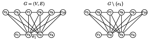
Figure 1: Toy example of extremal anomaly detection discussed in Section 3.3. The given graph $G=(V,E)$ has $|V|=10$ nodes, $|E|=20$ edges and $\alpha=16$ triangles ($3$-cycles) giving $\mathfrak{C}^{2}_{3}(G)=|V|-|E|+\alpha=6$, where the densest subgraph of $G$ is the subgraph node-induced by the nodes $V\setminus\{v_{1},v_{4}\}$ with $8$ nodes and $18$ edges giving $\rho(G)=\nicefrac{{18}}{{8}}=\nicefrac{{9}}{{4}}$. The graph $G\setminus\{e_{1}\}$ has $|E\setminus\{e_{1}\}|=19$ edges and $\alpha^{\prime}=10$ triangles giving $\mathfrak{C}^{2}_{3}(G\setminus\{e_{1}\})=|V|-|E\setminus\{e_{1}\}|+\alpha^{\prime}=1$. However, it can be verified that more than four edges will need to be deleted from $G$ to bring down the value of $\rho(G)$ to at most $\nicefrac{{27}}{{16}}$.

Targeted anomaly detection for a dynamic biological network

Figure 2: Toy example of targeted anomaly detection discussed in Section 3.3. (a) The original dynamical system with four observable output variables. (b) Values of the four output variable over time starting with an all-zero initial condition. (c) The thresholding rules employed to binarize the expression values in (b) as captured by a DNA microarray. (d) The reverse-engineered network for two successive time steps.

Consider the targeted anomaly detection problem (Problem Tadp in Section 5.2) using the Gromov-hyperbolic curvature (Definition 2). Suppose that we have a biological dynamical system of $4$ variables $x_{1},x_{2},x_{3},x_{4}$ generated by a set of recurrence equations as shown in Fig. 2 (a) for $x_{1}(t),x_{2}(t),x_{3}(t)$ and $x_{4}(t)$ as a function of discrete time $t=0,1,2,3,\dots\dots$, with the initial condition of $x_{1}(0)=x_{2}(0)=x_{3}(0)=x_{4}(0)=0$. Note that in this biological system any change in the value of $x_{1}$ affects $x_{4}$ with a delay. These recurrence equations are not known to the observer, but they generate a sequence of real values of the state variables for each successive discrete time units (shown in Fig. 2 (b) for $t=2$ and $t=3$). Suppose that an observer measures a binarized version of these real values of the state variables for each successive discrete time units using a DNA microarray by using thresholds as shown in Fig. 2 (c), and then reverse-engineers a time-varying network by using the hitting-set approach of Krupa (DL16, , Section 5.4.2)Jarrah with a time delay of $2$ (the corresponding network for $t=2$ and $t=3$ is shown in Fig. 2 (d)). Suppose that for our targeted anomaly detection problem we fix our attention to the two graphs $G_{2}$ and $G_{1}$ constructed in the two successive time steps $t=2$ and $t=3$, respectively, where $G_{2}=G_{1}\setminus\big{\{}\{x_{1},x_{4}\},\{x_{3},x_{4}\}\big{\}}$ is the target graph. It can be easily verified that $\mathfrak{C}_{\mathrm{Gromov}}(G_{1})=\rho(G_{1})=1$, $\mathfrak{C}_{\mathrm{Gromov}}(G_{2})=0$, and $\rho(G_{2})=\nicefrac{{1}}{{2}}$. Since $\mathfrak{C}_{\mathrm{Gromov}}(G_{1}\setminus\{x_{1},x_{4}\})=0$ it follows that we only need to delete the edge $\{x_{1},x_{4}\}$ to bring down the value of $\mathfrak{C}_{\mathrm{Gromov}}(G_{1})$ to $\mathfrak{C}_{\mathrm{Gromov}}(G_{2})$. However, both the edges $\{x_{1},x_{4}\}$ and $\{x_{3},x_{4}\}$ need to be deleted from $G_{1}$ to bring down the value of $\rho(G_{1})$ to $\rho(G_{2})$.

3.4 Brief remarks regarding the limitations of our theoretical results

Our theoretical results obviously have some limitations, specially for real-world networks. For example, our inapproximability results for the Gromov-hyperbolic curvature require a high average node degree. Thus, for real-world networks such as scale-free networks the inapproximability bounds may not apply. On another note, for geometric curvatures we only considered the first-order non-trivial measure $\mathfrak{C}^{2}_{d}$, but perhaps more salient non-trivial topological properties could be captured by using $\mathfrak{C}^{p}_{d}$ for $p>2$.

4 Two notions of graph curvature

For this paper, a curvature for a graph $G$ is a function $\mathfrak{C}\stackrel{{\scriptstyle\mathrm{def}}}{{=}}\mathfrak{C}(G):G\mapsto{\mathbb{R}}$. There are several ways in which network curvature can be defined depending on the type of global properties the measure is desired to affect; in this paper we consider two such definitions as described subsequently.

4.1 Gromov-hyperbolic curvature

This measure for a metric space was first suggested by Gromov in a group theoretic context G87 . The measure was first defined for infinite continuous metric space book , but was later also adopted for finite graphs. Usually the measure is defined via geodesic triangles as stated in Definition 2. For this definition, it would be useful to consider the given graph $G$ as a metric graph, i.e., we identify (by an isometry) any edge $\{u,v\}\in E$ with the real interval $[0,1]$ and thus any point in the interior of the edge $\{u,v\}$ can also be thought as a (virtual) node of $G$. Define a geodesic triangle $\Delta_{u,v,w}$ to be an ordered triple of three shortest paths $(\overline{u,v}$, $\overline{u,w}$ and $\overline{v,w})$ for the three nodes $u,v,w$ in $G$.

Definition 2 (Gromov-hyperbolic curvature measure via geodesic triangles)

For a geodesic triangle $\Delta_{u,v,w}$, let $\mathfrak{C}_{\mathrm{Gromov}}(\Delta_{u,v,w})$ be the minimum number such that $\overline{u,v}$ lies in a $\mathfrak{C}_{\mathrm{Gromov}}(\Delta_{u,v,w})$-neighborhood of $\overline{u,w}\,\cup\,\overline{v,w}$, i.e., for every node $x$ on $\overline{u,v}$, there exists a node $y$ on $\overline{u,w}$ or $\overline{v,w}$ such that $\mathrm{dist}_{G}(x,y)\leq\mathfrak{C}_{\mathrm{Gromov}}(\Delta_{u,v,w})$. Then the graph $G$ has a Gromov-hyperbolic curvature (or Gromov hyperbolicity) of $\mathfrak{C}_{\mathrm{Gromov}}\stackrel{{\scriptstyle\mathrm{def}}}{{=}}\mathfrak{C}_{\mathrm{Gromov}}(G)$ where $\mathfrak{C}_{\mathrm{Gromov}}(G)=\min\limits_{u,v,w\in V}\left\{\mathfrak{C}_{\mathrm{Gromov}}(\Delta_{u,v,w})\right\}$.

An infinite collection $\mathcal{G}$ of graphs belongs to the class of $\mathfrak{C}_{\mathrm{Gromov}}$-Gromov-hyperbolic graphs if and only if any graph $G\in\mathcal{G}$ has a Gromov-hyperbolic curvature of $\mathfrak{C}_{\mathrm{Gromov}}$. Informally, any infinite metric space has a finite value of $\mathfrak{C}_{\mathrm{Gromov}}$ if it behaves metrically in the large scale as a negatively curved Riemannian manifold, and thus the value of $\mathfrak{C}_{\mathrm{Gromov}}$ can be related to the other standard curvatures of a hyperbolic manifold. For example, a simply connected complete Riemannian manifold whose sectional curvature is below $\alpha<0$ has a value of $\mathfrak{C}_{\mathrm{Gromov}}=O\big{(}\sqrt{-\alpha}\,\big{)}$ (see R96 ). This is a major justification of using $\mathfrak{C}_{\mathrm{Gromov}}$ as a notion of curvature of any metric space.

Let $\omega$ be the value such that two $n\times n$ matrices can be multiplied in $O(n^{\omega})$ time; the smallest current value of $\omega$ is about $2.373$ VVW12 . Then the following results computational complexity results are known for computing $\mathfrak{C}_{\mathrm{Gromov}}(G)$ for an $n$-node graph $G$.

1. $\mathfrak{C}_{\mathrm{Gromov}}(G)$ can be exactly computed in $O\left(n^{\frac{5+\omega}{2}}\right)=O\left(n^{3.687}\right)$ time ipl15 .

2. $(1+\varepsilon)$-approximation of $\mathfrak{C}_{\mathrm{Gromov}}(G)$ can be computed in
   $\tilde{O}\left(\frac{1}{\varepsilon}n^{1+\omega}\right)=\tilde{O}\left(\frac{1}{\varepsilon}n^{3.373}\right)$ time Du14 , and $(2+\varepsilon)$-approximation of
   $\mathfrak{C}_{\mathrm{Gromov}}(G)$ can be computed in $\tilde{O}\left(\frac{1}{\varepsilon}n^{\omega}\right)=\tilde{O}\left(\frac{1}{\varepsilon}n^{2.373}\right)$ time Du14 .

3. $8$-approximation of $\mathfrak{C}_{\mathrm{Gromov}}(G)$ can be computed in $O\left(n^{2}\right)$ time CCDDMV18 .

It is easy to see that if $G$ is a tree then $\mathfrak{C}_{\mathrm{Gromov}}(G)=0$. Other examples of graph classes for which $\mathfrak{C}_{\mathrm{Gromov}}(G)$ is a small constant include chordal graphs, cactus of cliques, AT-free graphs, link graphs of simple polygons, and any class of graphs with a fixed diameter. A small value of Gromov-hyperbolicity is often crucial for algorithmic designs; for example, several routing-related problems or the diameter estimation problem become easier for networks with small $\mathfrak{C}_{\mathrm{Gromov}}$ values CE07 ; CDEHV08 ; CDEHVX12 ; GL05 . There are many well-known measures of curvature of a continuous surface or other similar spaces (e.g., curvature of a manifold) that are widely used in many branches of physics and mathematics. It is possible to relate Gromov-hyperbolic curvature to such other curvature notions indirectly via its scaled version, e.g., see JLB07 ; NS11 ; JLA11 .

4.1.1 Gromov-hyperbolic curvature and real-world networks

Recently, there has been a surge of empirical works measuring and analyzing the Gromov curvature $\mathfrak{C}_{\mathrm{Gromov}}$ of networks, and many real-world networks (e.g., preferential attachment networks, networks of high power transceivers in a wireless sensor network, communication networks at the IP layer and at other levels) were observed to have a small constant value of $\mathfrak{C}_{\mathrm{Gromov}}$ NS11 ; PKBV10 ; JL04 ; JLB07 ; ALJKZ08 . The authors in ADM14 analyzed $11$ well-known biological networks and $9$ well-known social networks for their $\mathfrak{C}_{\mathrm{Gromov}}$ values and found all but one network had a statistically significant small value of $\mathfrak{C}_{\mathrm{Gromov}}$. These references also describe implications of range of $\mathfrak{C}_{\mathrm{Gromov}}$ on the actual real-world applications of these networks. As mentioned in the following subsection, the Gromov-hyperbolicity measure is fundamentally different from the commonly used topological properties for a graph; for example, it is neither a hereditary nor a monotone property, is not the same as tree-width measure or other standard combinatorial properties that are commonly used in the computer science literature, and not necessarily a measure of closeness to tree topology.

4.1.2 Some clarifying remarks regarding Gromov-hyperbolicity measure

As pointed out in details by the authors in (DKMY18, , Section 1.2.1), the Gromov-hyperbolicity measure $\mathfrak{C}_{\mathrm{Gromov}}$ enjoys many non-trivial topological characteristics. In particular, the authors in (DKMY18, , Section 1.2.1) point out the following:

1. $\mathfrak{C}_{\mathrm{Gromov}}$ is not a hereditary or monotone property since removal of nodes or edges may change the value of $\mathfrak{C}_{\mathrm{Gromov}}$ sharply.

2. $\mathfrak{C}_{\mathrm{Gromov}}$ is not necessarily the same as tree-width measure (see also MSV11 ; ADM14 ), or other standard combinatorial properties (e.g., betweenness centrality, clustering coefficient, dense sub-graphs) that are commonly used in the computer science literature.

3. “Close to hyperbolic topology” is not necessarily the same as “close to tree topology”.

4.2 Geometric curvatures

In this section, we describe geometric curvatures of graphs by using correspondence with topological objects in higher dimension. The approach of using associations of sub-graphs with with topological objects in higher dimension has also been used in some previous papers such as WJS16 but our anomaly detection approach is quite different from them.

4.2.1 Basic topological concepts

We first review some basic concepts from topology; see introductory textbooks such as H94 ; GG99 for further information. Although not absolutely necessary, the reader may find it useful to think of the underlying metric space as the $r$-dimensional real space ${\mathbb{R}}^{r}$ be for some integer $r>1$.

1. A subset $S\subseteq{\mathbb{R}}^{r}$ is convex if and only if for any $x,y\in S$, the convex combination of $x$ and $y$ is also in $S$.

2. A set of $k+1$ points $x_{0},\dots,x_{k}\in{\mathbb{R}}^{r}$ are called affinely independent if and only if for all $\alpha_{0},\dots,\alpha_{k}\in{\mathbb{R}}$ $\sum_{j=0}^{k}\alpha_{j}x_{j}=0$ and $\sum_{j=0}^{k}\alpha_{j}=0$ implies $\alpha_{0}=\dots=\alpha_{k}=0$.

3. The $k$-simplex generated by a set of $k+1$ affinely independent points $x_{0},\dots,x_{k}\in{\mathbb{R}}^{r}$ is the subset $\mathcal{S}\big{(}x_{0},\dots,x_{k}\big{)}$ of ${\mathbb{R}}^{r}$ generated by all convex combinations of $x_{0},\dots,x_{k}$.

   1. Each $(\ell+1)$-subset $\big{\{}x_{i_{0}},\dots,x_{i_{\ell}}\big{\}}\subseteq\big{\{}x_{0},\dots,x_{k}\big{\}}$ defines the $\ell$-simplex $\mathcal{S}\big{(}x_{i_{0}},\dots,x_{i_{\ell}}\big{)}$ that is called a face of dimension $\ell$ (or a $\ell$-face) of $\mathcal{S}\big{(}x_{0},\dots,x_{k}\big{)}$. A $(k-1)$-face, $1$-face and $0$-face is called a facet, an edge and a node, respectively.

4. A (closed) halfspace is a set of points satisfying $\sum_{j=1}^{r}a_{j}x_{j}\leq b$ for some $a_{1},\dots,a_{r},b\in{\mathbb{R}}$. The convex set obtained by a bounded non-empty intersection of a finite number of halfspaces is called a convex polytope (convex polygon in two dimensions).

   1. If the intersection of a halfspace and a convex polytope is a subset of the halfspace then it is called a face of the polytope. Of particular interests are faces of dimensions $r-1$, $1$ and $0$, which are called facets, edges and nodes of the polytope, respectively.

5. A simplicial complex (or just a complex) is a topological space constructed by the union of simplexes via topological associations.

4.2.2 Geometric curvature definitions

Informally, a complex is “glued” from nodes, edges and polygons via topological identification. We first define $k$-complex-based Forman’s combinatorial Ricci curvature for elementary components (such as nodes, edges, triangles and higher-order cliques) as described in Bl14 ; Fo03 ; WJS16 ; WSJ16 , and then obtain a scalar curvature that takes an appropriate linear combination of these values (via Gauss-Bonnet type theorems, see for example (WSJ16, , Sections $4.1$–$4.3$) and the references therein) that correspond to the so-called Euler characteristic of the complex that is topologically associated with the given graph. In this paper, we consider such Euler characteristics of a graph to define geometric curvature.

To begin the topological association, we (topologically) associate a $q$-simplex with a $(q+1)$-clique $\mathcal{K}_{q+1}$; for example, $0$-simplexes, $1$-simplexes, $2$-simplexes and $3$-simplexes are associated with nodes, edges, $3$-cycles (triangles) and $4$-cliques, respectively. Next, we would also need the concept of an “order” of a simplex for more non-trivial topological association. Consider a $p$-face $f^{p}$ of a $q$-simplex. An order $d$ association of such a face, which we will denote by the notation $f_{d}^{p}$ with the additional subscript $d$, is associated with a sub-graph of at most $d$ nodes that is obtained by starting with $\mathcal{K}_{p+1}$ and then optionally replacing each edge by a path between the two nodes. For example,

• $f_{d}^{0}$ is a node of $G$ for all $d\geq 1$.

• $f_{2}^{1}$ is an edge, and $f_{d}^{1}$ for $d>2$ is a path having at most $d$ nodes between two nodes adjacent in $G$.

• $f_{3}^{2}$ is a triangle (cycle of $3$ nodes or a $3$-cycle), and $f_{d}^{2}$ for $d>3$ is obtained from $3$ nodes by connecting every pair of nodes by a path such that the total number of nodes in the sub-graph is at most $d$.

Naturally, the higher the values of $p$ and $q$ are, the more complex are the topological associations. Let $\mathcal{F}_{d}^{k}$ be the set of all $f_{d}^{k}$’s that are topologically associated. With such associations via $p$-faces of order $d$, the Euler characteristics of the graph $G=(V,E)$ and consequently the curvature can be defined as

$$\mathfrak{C}^{p}_{d}(G)\stackrel{{\scriptstyle\mathrm{def}}}{{=}}\sum\limits_{k=0}^{p}(-1)^{k}\,\left|\mathcal{F}_{d}^{k}\right|$$ (1)

It is easy to see that both $\mathfrak{C}^{0}_{d}(G)$ and $\mathfrak{C}^{1}_{d}(G)$ are too simplistic to be of use in practice. Thus, we consider the next higher value of $p$ in this paper, namely when $p=2$. Letting $\mathcal{C}(G)$ denote the number of cycles of at most $d+1$ nodes in $G$, we get the measure

$$\mathfrak{C}^{2}_{d}(G)=|V|-|E|+|\mathcal{C}(G)|$$

Suitability of geometric curvature measures for real-world networks: The usefulness of geometric curvatures for real-world networks was demonstrated in publications such as WJS16 ; WSJ16 ; SSG18 .

5 Formalizations of two anomaly detection problems on networks

In this section, we formalize two versions of the anomaly detection problem on networks. An underlying assumption on the behind these formulations is that the graph adds/deletes edges only while keeping the same set of nodes.

5.1 Extremal anomaly detection for static networks

The problems in this subsection are motivated by a desire to quantify the extremal sensitivity of static networks. The basic decision question is: “is there a subset among a set of prescribed edges whose deletion may change the network curvature significantly?”. This directly leads us to the following decision problem:

Problem name:	Extremal Anomaly Detection Problem
	(Eadp${}_{\mathfrak{C}}(G,\widetilde{E},\gamma)$)
Input:	$\bullet$ A curvature measure $\mathfrak{C}:G\mapsto{\mathbb{R}}$
	$\bullet$ A connected graph $G=(V,E)$,
	an edge subset $\widetilde{E}\subseteq E$ such that $G\setminus\widetilde{E}$ is connected,
	and a real number $\gamma<\mathfrak{C}(G)$ (resp., $\gamma>\mathfrak{C}(G)$)
Decision question :	is there an edge subset $\widehat{E}\subseteq\widetilde{E}$ such that $\mathfrak{C}(G\setminus\widehat{E})\leq\gamma$
	(resp., $\mathfrak{C}(G\setminus\widehat{E})\geq\gamma$) ?
Optimization question :	if the answer to the decision question is “yes”           then minimize $|\widehat{E}|$
Notation:	if the answer to the decision question is “yes” then
	the minimum possible value of $|\widehat{E}|$
	is denoted by $\mathsf{OPT}_{\mbox{{\sc Eadp}}_{\mathfrak{C}}}(G,\widetilde{E},\gamma)$

The following comments regarding the above formulation should be noted:

1. For the case $\gamma<\mathfrak{C}(G)$ (resp., $\gamma>\mathfrak{C}(G)$) we allow $\mathfrak{C}(G\setminus\widetilde{E})>\gamma$ (resp., $\mathfrak{C}(G\setminus\widetilde{E})<\gamma$), thus $\widehat{E}=\widetilde{E}$ need not be a feasible solution at all.

2. The curvature function is only defined for connected graphs, thus we require $G\setminus\widetilde{E}$ to be connected.

3. The edges in $E\setminus\widetilde{E}$ can be thought of as “critical” edges needed for the functionality of the network. For example, in the context of inference of minimal biological networks from indirect experimental evidences ADDKSZW07 ; ADDS , the set of critical edges represent direct biochemical interactions with concrete evidence.

5.2 Targeted anomaly detection for dynamic networks

These problems are primarily motivated by change-point detections between two successive discrete time steps in dynamic networks AC17 ; KS09 , but they can also be applied to static networks when a subset of the final desired network is known. Fig. 2 illustrates targeted anomaly detection for a dynamic biological network.

Problem name :	Targeted Anomaly Detection Problem (Tadp${}_{\mathfrak{C}}(G_{1},G_{2})$)
Input:	$\bullet$ Two connected graphs $G_{1}=(V,E_{1})$ and $G_{2}=(V,E_{2})$
	with $E_{2}\subset E_{1}$
	$\bullet$ A curvature measure $\mathfrak{C}:G\mapsto{\mathbb{R}}$
Valid solution :	an edge subset $E_{3}\subseteq E_{1}\setminus E_{2}$ such that $\mathfrak{C}(G_{1}\setminus E_{3})=\mathfrak{C}(G_{2})$.
Objective:	minimize $|E_{3}|$.
Notation:	the minimum value of $|E_{3}|$         is denoted by $\mathsf{OPT}_{\mbox{{\sc Tadp}}_{\mathfrak{C}}}(G_{1},G_{2})$

6 Computational complexity of extremal anomaly detection problems

6.1 Geometric curvatures: computational complexity of Eadp${}_{\mathfrak{C}^{2}_{d}}$

Theorem 6.1

(a) The following statements hold for Eadp${}_{\mathfrak{C}^{2}_{d}}(G,\widetilde{E},\gamma)$ when $\gamma>\mathfrak{C}^{2}_{d}(G)$:

(a1)

We can decide in polynomial time the answer to the decision question (i.e., if there exists any feasible solution $\widehat{E}$ or not).

(a2)

If a feasible solution exists then the following results hold:

(a2-1)

Computing $\mathsf{OPT}_{\mbox{{\sc Eadp}}_{\mathfrak{C}^{2}_{d}}}(G,\widetilde{E},\gamma)$ is $\mathsf{NP}$-hard for all $d$ that are multiple of $3$.

(a2-2)

If $\gamma$ is sufficient larger than $\mathfrak{C}^{2}_{d}(G)$ then we can design an approximation algorithm that approximates both the cardinality of the minimal set of edges for deletion and the absolute difference between the two curvature values. More precisely, if $\gamma\geq\mathfrak{C}^{2}_{d}(G)+\left(\frac{1}{2}+\varepsilon\right)(2|\widetilde{E}|-|E|)$ for some $\varepsilon>0$, then we can find in polynomial time a subset of edges $E_{1}\subseteq\widetilde{E}$ such that

$$|E_{1}|\leq 2\,\mathsf{OPT}_{\mbox{{\sc Eadp}}_{\mathfrak{C}^{2}_{d}}}(G,\widetilde{E},\gamma)\text{ and }\frac{\mathfrak{C}^{2}_{d}(G\setminus E_{1})-\mathfrak{C}^{2}_{d}(G)}{\gamma-\mathfrak{C}^{2}_{d}(G)}\geq\frac{4\varepsilon}{1+2\varepsilon}$$

(b) The following statements hold for Eadp${}_{\mathfrak{C}^{2}_{d}}(G,\widetilde{E},\gamma)$ when $\gamma<\mathfrak{C}^{2}_{d}(G)$:

(b1)

We can decide in polynomial time the answer to the decision question (i.e., if there exists any feasible solution $\widehat{E}$ or not).

(b2)

If a feasible solution exists and $\gamma$ is not too far below $\mathfrak{C}^{2}_{d}(G)$ then we can design an approximation algorithm that approximates both the cardinality of the minimal set of edges for deletion and the absolute difference between the two curvature values. More precisely, letting $\Delta$ denote the number of cycles of $G$ of at most $d+1$ nodes that contain at least one edge from $\widetilde{E}$, if $\gamma\geq\mathfrak{C}^{2}_{d}(G)-\frac{\Delta}{1+\varepsilon}$ for some $\varepsilon>0$ then we can find in polynomial time a subset of edges $E_{1}\subseteq\widetilde{E}$ such that

$$|E_{1}|\leq 2\,\mathsf{OPT}_{\mbox{{\sc Eadp}}_{\mathfrak{C}^{2}_{d}}}(G,\widetilde{E},\gamma)\text{ and }\frac{\mathfrak{C}^{2}_{d}(G\setminus E_{1})-\mathfrak{C}^{2}_{d}(G)}{\gamma-\mathfrak{C}^{2}_{d}(G)}\leq 1-\varepsilon$$

(b3)

If $\gamma<\mathfrak{C}^{2}_{d}(G)$ then, even if $\gamma=\mathfrak{C}^{2}_{d}(G\setminus\widetilde{E})$ (i.e., a trivial feasible solution exists), computing $\mathsf{OPT}_{\mbox{{\sc Eadp}}_{\mathfrak{C}^{2}_{d}}}(G,\widetilde{E},\gamma)$ is at least as hard as computing Tadp${}_{\mathfrak{C}^{2}_{d}}(G_{1},G_{2})$ and therefore all the hardness results for Tadp${}_{\mathfrak{C}^{2}_{d}}(G_{1},G_{2})$ in Theorem 7.1 also apply to $\mathsf{OPT}_{\mbox{{\sc Eadp}}_{\mathfrak{C}^{2}_{d}}}(G,\widetilde{E},\gamma)$.

6.1.1 Proof techniques and relevant comments regarding Theorem 6.1

(on proofs of (a1) and (b1))

After eliminating a few “easy-to-solve” sub-cases, we prove the remaining cases of (a1) and (b1) by reducing the feasibility questions to suitable minimum-cut problems; the reductions and proofs are somewhat different due to the nature of the objective function. It would of course be of interest if a single algorithm and proof can be found that covers both instances and, more importantly, if a direct and more efficient greedy algorithm can be found that avoids the maximum flow computation.

(on proofs of (a2-2) and (b2))

Our general approach to prove (a2-2) and (b2) is to formulate these problems as a series of (provably $\mathsf{NP}$-hard and polynomially many) “constrained” minimum-cut problems. We start out with two different (but well-known) polytopes for the minimum cut problem (polytopes (10) and (10)^′). Even though the polytope (10)^′ is of exponential size for general graphs, it is of polynomial size for our particular minimum cut version and so we do not need to appeal to separation oracles for its efficient solution. We subsequently add extra constraints corresponding to a parameterized version of the minimization objective and solve the resulting augmented polytopes (polytopes (18) and (18)^′) in polynomial time to get a fractional solution and use a simple deterministic rounding scheme to obtain the desired bounds.

1. Our algorithmic approach uses a sequence of $\lceil\log_{2}(1+|\widetilde{E}|)\rceil=O(\log|E|)$ linear-programming ($\mathsf{LP}$) computations by using an obvious binary search over the relevant parameter range. It would be interesting to see if we can do the same using $O(1)$ $\mathsf{LP}$ computations.

2. Is the factor $2$ in “$|E_{1}|\leq 2\,\mathsf{OPT}_{\mbox{{\sc Eadp}}_{\mathfrak{C}^{2}_{d}}}(G,\widetilde{E},\gamma)$” an artifact of our specific rounding scheme around the threshold of $\nicefrac{{1}}{{2}}$ and perhaps can be improved using a cleverer rounding scheme? This seems unlikely for the case when $\gamma<\mathfrak{C}^{2}_{d}(G)$ since the inapproximability results in (b3) include a $(2-\varepsilon)$-inapproximability assuming the unique games conjecture is true. However, this possibility cannot be ruled out for the case when $\gamma>\mathfrak{C}^{2}_{d}(G)$ since we can only prove $\mathsf{NP}$-hardness for this case.

3. There are subtle but crucial differences between the rounding schemes for (a2-2) and (b2) that is essential to proving the desired bounds. To illustrate this, consider an edge $e$ with a fractional value of $\nicefrac{{1}}{{2}}$ for its corresponding variable. In the rounding scheme (21) of (a2-2) $e$ will only sometimes be designated as a cut edge, whereas in the rounding scheme (21)^′ of (b2) $e$ will always be designated as a cut edge.

(on the bounds over $\boldsymbol{\gamma}$ in (a2-2)

If $|\widetilde{E}|\lessapprox\frac{1}{2}|E|$ then the condition on $\gamma$ is redundant (i.e., always holds). Thus indeed the $2$-approximation is likely to hold unconditionally for practical applications of this problem since anomaly is supposed to be caused by a large change in curvature by a relatively small number of elementary components (edges in our cases).

Furthermore, if $|E|\leq 2|V|$ then the condition on $\gamma$ always holds irrespective of the value of $|\widetilde{E}|$, and the smaller is $|\widetilde{E}|$ with respect to $|E|$ the better is our approximation of the curvature difference. As a general illustration, when $\varepsilon=\nicefrac{{1}}{{5}}$ the assumptions are $\gamma\geq\mathfrak{C}^{2}_{d}(G)+\frac{7}{10}(2|\widetilde{E}|-|E|)$, and the corresponding bounds are $|E_{1}|\leq 2\,\mathsf{OPT}_{\mbox{{\sc Eadp}}_{\mathfrak{C}^{2}_{d}}}(G,\widetilde{E},\gamma)\,\,\,\,\text{and}\,\,\,\,\frac{\mathfrak{C}^{2}_{d}(G\setminus E_{1})-\mathfrak{C}^{2}_{d}(G)}{\gamma-\mathfrak{C}^{2}_{d}(G)}\geq\frac{4}{7}$.

(on the hardness proof in (a2-1))

Our reduction is from the densest-$k$-subgraph (D$k$S₃) problem. We use the reduction from the CLIQUE problem to D$k$S₃ detailed by Feige and Seltser in FS97 which shows that D$k$S₃ is $\mathsf{NP}$-hard even if the degree of every node is at most $3$. For convenience in doing calculations, we use the reduction of Feige and Seltser starting from the still $\mathsf{NP}$-hard version of the CLIQUE problem where the input instances are $(n-4)$-regular $n$-node graphs. Pictorially, the reduction is illustrated in Fig. 3. Note that D$k$S₃ is not known to be $(1+\varepsilon)$-inapproximable assuming P$\neq\mathsf{NP}$ (though it is likely to be), and thus our particular reduction cannot be generalized to $(1+\varepsilon)$-inapproximability assuming P$\neq\mathsf{NP}$.

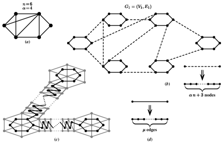
Figure 3: Illustration of the reduction in the proof of Theorem 6.1(a2-1). (a) The original instance of the $\alpha$-CLIQUE problem on an $n$-node graph. (b) Illustration of the $\mathsf{NP}$-hardness reduction from $\alpha$-CLIQUE to D$k$S₃ by Feige and Seltser FS97 . (c) Illustration of associations of nodes with unique $3$-cycles such that an edge between two nodes are adjacent correspond to sharing an unique edge of their associated $3$-cycles. (d) Splitting of every edge of $G_{1}$ into a path of $\mu$ edges for the case when $d=3\mu$ for some integer $\mu>1$.

6.1.2 Proof of Theorem 6.1

Proof of (a1)

Let the notation $\mathcal{C}(H)$ denote the set of cycles having at most $d+1$ nodes in a graph $H$. Assume $\Delta=|\mathcal{C}(G)|$ and let $\mathcal{C}(G)=\{\mathcal{F}_{1},\mathcal{F}_{2},\dots,\mathcal{F}_{\Delta}\}$; thus $\mathfrak{C}^{2}_{d}(G)=n-m+\Delta$ where $|V|=n$ and $|E|=m$. Since $d$ is fixed, $\Delta=O(n^{d})$ and all the cycles in $\mathcal{C}(G)$ can be explicitly enumerated in polynomial ($O(n^{d})$) time. Let $\mathcal{C}^{\prime}(G)=\{\mathcal{F}_{1},\mathcal{F}_{2},\dots,\mathcal{F}_{\Delta^{\prime}}\}\subseteq\mathcal{C}(G)$ be the set of $\Delta^{\prime}\leq\Delta$ cycles in $\mathcal{C}(G)$ that involve one of more edges from $\widetilde{E}$. An overview of the main steps in our proof for (a1) is as follows.

1. We identify sub-cases that are easy to solve.

2. For all remaining sub-cases, we reduce our problem to a standard

(directed) minimum $$s t$$- cut problem such that the following

statements hold:

$$\triangleright$$ The cut network can be constructed in polynomial time.

$$\triangleright {}_{\mathfrak{C}^{2}_{d}}(G,\widetilde{E},\gamma)$$ There exists a feasible solution of Eadp if and

only if the minimum cut value is at most $$\Gamma\stackrel{{\scriptstyle\mathrm{def}}}{{=}}\mathfrak{C}^{2}_{d}(G)-\gamma+|\widetilde{E}|$$.

Step 1. Identifying sub-cases that are easy to solve

We first observe that the following sub-cases are easy to solve:

• If $\gamma>n-(m-|\widetilde{E}|)+\Delta$ then we can assert that there is no feasible solution. This is true because for any $E^{\prime}\subseteq\widetilde{E}$ it is true that $\mathfrak{C}^{2}_{d}(G\setminus E^{\prime})$ is at most $n-(m-|\widetilde{E}|)+\Delta$.

• If $\gamma\leq n-(m-|\widetilde{E}|)+\Delta$ and $\Delta^{\prime}=0$ then there exists a trivial optimal feasible solution of the following form:

  select any set of $m_{1}$ edges from $\widetilde{E}$ where $m_{1}$ is the least positive integer satisfying $n-(m_{1}-|\widetilde{E}|)+\Delta\geq\gamma$.

Step 2. Solving all remaining sub-cases

We assume that $\gamma\leq n-(m-|\widetilde{E}|)+\Delta$ and $\Delta^{\prime}>0$. Consider a subset $E_{1}\subseteq\widetilde{E}$ of $m_{1}=|E_{1}|\leq|\widetilde{E}|$ edges for deletion and suppose that removal of the edges in $E_{1}$ removes $\Delta_{1}\leq\Delta^{\prime}$ cycles from $\mathcal{C}^{\prime}(G)$ (i.e., $|\mathcal{C}^{\prime}(G\setminus E_{1})|=\Delta^{\prime}-\Delta_{1}$). Then,

$$\mathfrak{C}^{2}_{d}(G\setminus E_{1})=n-(m-m_{1})+(\Delta-\Delta_{1})\\ =n-m+\Delta+(m_{1}-\Delta_{1})=\mathfrak{C}^{2}_{d}(G)+(m_{1}-\Delta_{1})$$ (2)

and consequently one can observe that

$$\mathfrak{C}^{2}_{d}(G\setminus E_{1})\geq\gamma\,\equiv\,m_{1}-\Delta_{1}\geq\gamma-\mathfrak{C}^{2}_{d}(G)\,\equiv\,\Delta_{1}-m_{1}\leq\mathfrak{C}^{2}_{d}(G)-\gamma\\ \equiv\,\Delta_{1}+(m-m_{1})\leq\mathfrak{C}^{2}_{d}(G)-\gamma+m\,\equiv\,\Delta_{1}+(|\widetilde{E}|-m_{1})\leq\mathfrak{C}^{2}_{d}(G)-\gamma+|\widetilde{E}|\stackrel{{\scriptstyle\mathrm{def}}}{{=}}\Gamma$$ (3)

Note that $\Gamma=\mathfrak{C}^{2}_{d}(G)-\gamma+|\widetilde{E}|=n-(m-|\widetilde{E}|)+\Delta-\gamma\geq 0$ and $|\widetilde{E}|-m_{1}$ is the number of edges in $\widetilde{E}$ that are not in $E_{1}$ and therefore not selected for deletion. Also, note that $\Gamma$ is a quantity that depends on the problem instance only and does not change if one or more edges are deleted. Based on this interpretation, we construct the following instance (digraph) $\mathcal{G}=(\mathcal{V},\mathcal{E})$ of a (standard directed) minimum $s$-$t$ cut problem (where $\mathrm{cap}(u,v)$ is the capacity of a directed edge $(u,v)$):

• The nodes in $\mathcal{V}$ are as follows: a source node $s$, a sink node $t$, a node (an “edge-node”) $u_{e}$ for every edge $e\in\widetilde{E}$ and a node (a “cycle-node”) $u_{\mathcal{F}_{i}}$ for every cycle $\mathcal{F}_{i}\in\mathcal{C}^{\prime}(G)$. The total number of nodes is therefore $O(|\widetilde{E}|+n^{d})$, i.e., polynomial in $n$.

• The directed edges in $\mathcal{E}$ and their corresponding capacities are as follows:

  • For every edge $e\in\widetilde{E}$, we have a directed edge $(s,u_{e})$ (an “edge-arc”) of capacity $\mathrm{cap}(s,u_{e})=1$.

  • For every cycle $\mathcal{F}_{i}\in\mathcal{C}^{\prime}(G)$, we have a directed edge (a “cycle-arc”) $(u_{\mathcal{F}_{i}},t)$ of capacity $\mathrm{cap}(u_{\mathcal{F}_{i}},t)=1$.

  • For every cycle $\mathcal{F}_{i}\in\mathcal{C}^{\prime}(G)$ and every edge $e\in\widetilde{E}$ such that $e$ is an edge of $\mathcal{F}_{i}$, we have a directed edge (an “ed-cy-arc”, ed-cy-arc for short) $(u_{e},u_{\mathcal{F}_{i}})$ of capacity $\mathrm{cap}(u_{e},u_{\mathcal{F}_{i}})=\infty$.

For an $s$-$t$ cut $(\mathcal{S},\mathcal{V}\setminus\mathcal{S})$ of $\mathcal{G}$ (where $s\in\mathcal{S}$ and $t\notin\mathcal{S}$), let $\mathrm{cut}(\mathcal{S},\mathcal{V}\setminus\mathcal{S})=\{(x,y)\,|\,x\in\mathcal{S},\,y\notin\mathcal{S}\}$ and $\mathrm{cap}(\mathrm{cut}(\mathcal{S},\mathcal{V}\setminus\mathcal{S}))=\sum_{(x,y)\in\mathrm{cut}(\mathcal{S},\mathcal{V}\setminus\mathcal{S})}\mathrm{cap}(x,y)$ denote the edges in the cut and the capacity of the cut, respectively. It is well-known how to compute a minimum $s$-$t$ cut of value
$\Phi\stackrel{{\scriptstyle\mathrm{def}}}{{=}}\min_{\emptyset\subset\mathcal{S}\subset\mathcal{V},\,s\in\mathcal{S},\,t\notin\mathcal{S}}\{\mathrm{cap}(\mathrm{cut}(\mathcal{S},\mathcal{V}\setminus\mathcal{S}))\}$ in polynomial time CCPS97 . The following lemma proves part (a1) of the theorem.

Lemma 1

There exists any feasible solution of Eadp${}_{\mathfrak{C}^{2}_{d}}(G,\widetilde{E},\gamma)$ if and only if $\Phi\leq\Gamma$. Moreover, if $(\mathcal{S},\mathcal{V}\setminus\mathcal{S})$ is a minimum $s$-$t$ cut of $\mathcal{G}$ of value $\Phi\leq\Gamma$ then $\widehat{E}=\{e\,|\,u_{e}\in\mathcal{S}\}$ is a feasible solution for Eadp${}_{\mathfrak{C}^{2}_{d}}(G,\widetilde{E},\gamma)$.

Proof

Suppose that there exists a feasible solution $E_{1}\subseteq\widetilde{E}$ with $m_{1}=|E_{1}|$ edges for Eadp${}_{\mathfrak{C}^{2}_{d}}(G,\widetilde{E},\gamma)$, and suppose that removal of the edges in $E_{1}$ removes $\Delta_{1}$ cycles from $\mathcal{C}^{\prime}(G)$. Consider the cut $(\mathcal{S},\mathcal{V}\setminus\mathcal{S})$ where

$$\mathcal{S}=\{s\}\bigcup\{u_{e}\,|\,e\in E_{1}\}\bigcup\left\{u_{\mathcal{F}_{i}}\,|\,\text{$\mathcal{F}_{i}$ contains at least one edge from $E_{1}$}\right\}$$

Note that no ed-cy-arc belongs to $\mathrm{cut}(\mathcal{S},\mathcal{V}\setminus\mathcal{S})$ and therefore

$$\mathrm{cap}(\mathrm{cut}(\mathcal{S},\mathcal{V}\setminus\mathcal{S}))\\ =|\{(s,u_{e})\,|\,e\notin E_{1}\}|+|\{(u_{\mathcal{F}_{i}},t)\,|\,\text{$\mathcal{F}_{i}$ contains at least one edge from $E_{1}$}\}|\\ =(|\widetilde{E}|-m_{1})+\Delta_{1}$$

and thus by Inequality (3) we can conclude that

$$\mathfrak{C}^{2}_{d}(G\setminus E_{1})\geq\gamma\\ \equiv\,\Delta_{1}+(|\widetilde{E}|-m_{1})\leq\Gamma\,\equiv\,\mathrm{cap}(\mathrm{cut}(\mathcal{S},\mathcal{V}\setminus\mathcal{S}))\leq\Gamma\,\Rightarrow\Phi\leq\mathrm{cap}(\mathrm{cut}(\mathcal{S},\mathcal{V}\setminus\mathcal{S}))\leq\Gamma$$

For the other direction, consider a minimum $s$-$t$ cut $(\mathcal{S},\mathcal{V}\setminus\mathcal{S})$ of $\mathcal{G}$ of value $\Phi\leq\Gamma$. Consider the solution $E_{1}=\{e\,|\,u_{e}\in\mathcal{S}\}\subseteq\widetilde{E}$ for Eadp${}_{\mathfrak{C}^{2}_{d}}(G,\widetilde{E},\gamma)$, and suppose that removal of the edges in $E_{1}$ removes $\Delta_{1}$ cycles from $\mathcal{C}^{\prime}(G)$. Since $\mathcal{G}$ admits a trivial $s$-$t$ cut $(\{s\},\mathcal{V}\setminus\{s\})$ of capacity $m_{1}<\infty$, no ed-cy-arc can be an edge of any minimum $s$-$t$ cut of $\mathcal{G}$, i.e., $\mathrm{cut}(\mathcal{S},\mathcal{V}\setminus\mathcal{S})$ contains only edge-arcs or cycle-arcs. Let $E_{2}=\{\mathcal{F}_{j}\,|\,u_{\mathcal{F}_{j}}\in\mathcal{S}\}$. Consider an edge $e\in E_{1}$ and let $\mathcal{F}_{j}$ be a cycle in $\mathcal{C}^{\prime}(G)$ containing $e$. Since $\mathrm{cut}(\mathcal{S},\mathcal{V}\setminus\mathcal{S})$ contains no ed-cy-arc, it does not contain the arc $(u_{e},u_{\mathcal{F}_{j}})$. It thus follows that the cycle-node $u_{\mathcal{F}_{j}}$ must also belong to $\mathcal{S}$ and thus $|E_{2}|=\Delta_{1}$. Now note that

$$\Phi=|\{u_{e}\,|\,u_{e}\notin\mathcal{S}\}|+|\{u_{\mathcal{F}_{j}}\,|\,u_{\mathcal{F}_{j}}\in\mathcal{S}\}|\\ =(|\widetilde{E}|-|E_{1}|)+\Delta_{1}\leq\Gamma=\mathfrak{C}^{2}_{d}(G)-\gamma+|\widetilde{E}|\\ \equiv\,\mathfrak{C}^{2}_{d}(G\setminus E_{1})=\mathfrak{C}^{2}_{d}(G)+|E_{1}|-\Delta_{1}\geq\gamma$$

This completes a proof for (a1).

Proof of (a2-2) We will reuse the proof of (a1) as appropriate. Let $\widehat{E}\subseteq\widetilde{E}$ be an optimal solution of the optimization version of Eadp${}_{\mathfrak{C}^{2}_{d}}(G,\widetilde{E},\gamma)$ having $\mathsf{OPT}_{\mbox{{\sc Eadp}}_{\mathfrak{C}^{2}_{d}}}(G,\widetilde{E},\gamma)$ nodes. Note that $\mathsf{OPT}_{\mbox{{\sc Eadp}}_{\mathfrak{C}^{2}_{d}}}(G,\widetilde{E},\gamma)\in\{1,2,\dots,|\widetilde{E}|\}$ and thus in polynomial time we can “guess” every possible value of
$\mathsf{OPT}_{\mbox{{\sc Eadp}}_{\mathfrak{C}^{2}_{d}}}(G,\widetilde{E},\gamma)$, solve the corresponding optimization problem with this additional constraint, and take the best of these solutions. In other words, it suffices if we can find, under the assumption that $\mathsf{OPT}_{\mbox{{\sc Eadp}}_{\mathfrak{C}^{2}_{d}}}(G,\widetilde{E},\gamma)=\kappa$ for some $\kappa\in\{1,2,\dots,|\widetilde{E}|\}$, find a solution $E_{1}\subseteq\widetilde{E}$ satisfying the claims in (a2-2). An overview of the main steps in our proof for (a2-2) is as follows (where the comments are enclosed within a pair of $(*$ and $*)$).

1. (* same as in (a1) *)

We identify sub-cases whose optimal solutions are easy to find.

Following steps apply only to all remaining sub-cases.

2. for $$\kappa=1,2,\dots,|\widetilde{E}| \mathsf{OPT}_{\mbox{{\sc Eadp}}_{\mathfrak{C}^{2}_{d}}}(G,\widetilde{E},\gamma)=\kappa$$ do       (* assume *)

2a. (* as in (a1) but with an additional constraint *)

we reduce our problem to a (directed) minimum $$s t$$- cut problem

with the following additional constraint

$$\blacktriangleright \widetilde{E} \kappa$$ the number of edges to be deleted from is

such that the following statements hold:

$$\triangleright$$ The cut network can be constructed in polynomial time.

$$\triangleright {}_{\mathfrak{C}^{2}_{d}}(G,\widetilde{E},\gamma)$$ There exists a feasible solution of Eadp

if and only if the minimum cut value is

at most $$\Gamma\stackrel{{\scriptstyle\mathrm{def}}}{{=}}\mathfrak{C}^{2}_{d}(G)-\gamma+|\widetilde{E}|$$.

2b. find an extreme-point optimal solution for an appropriate

polytope for the constrained minimum cut problem

in polynomial time.

2c. if the optimal objective value is at most $$\Gamma$$ then

2c(i). carefully convert relevant fractional values in the solution

to integral values to get a solution in polynomial time.

3. Return the best among all solutions found in Step 2

as the desired solution.

Step 2b. Formulating an appropriate polytope for the constrained minimum cut problem

We showed in the proof of part (a1) that the feasibility problem can be reduced to finding a minimum $s$-$t$ cut of the directed graph $\mathcal{G}=(\mathcal{V},\mathcal{E})$. Notice that $\mathcal{G}$ is acyclic, and every path between $s$ and $t$ has exactly three directed edges, namely an edge-arc followed by a ed-cy-arc followed by a cycle-arc. The minimum $s$-$t$ cut problem for a graph has a well-known associated convex polytope of polynomial size (e.g., see (V01, , pp. 98-99)). Letting $p_{\beta}$ to be the variable corresponding to each node $\beta\in\mathcal{V}$, and $d_{\alpha}$ to be the variable associated with the edge $\alpha\in\mathcal{E}$, this minimum $s$-$t$ cut polytope for the graph $\mathcal{G}$ is as follows:

minimize $$\sum_{\alpha\in\mathcal{E}}\mathrm{cap}(\alpha)d_{\alpha} =\sum_{{\alpha\in\mathcal{E},\text{\footnotesize$\alpha$ is not ed-cy-arc}}}d_{\alpha}+\sum_{{\alpha\in\mathcal{E},\text{\footnotesize$\alpha$ is ed-cy-arc}}}\infty\times d_{\alpha} d_{\alpha}\geq p_{\beta}-p_{\xi} \alpha=(\beta,\xi)\in\mathcal{E} p_{s}-p_{t}\geq 1 0\leq p_{\beta}\leq 1 \beta\in\mathcal{V} 0\leq d_{\alpha}\leq 1 \alpha\in\mathcal{E}$$ subject to      for every edge         for every node         for every edge (10)

It is well-known that all extreme-point solutions of (10) are integral. An integral solution of (10) generates a $s$-$t$ cut $(\mathcal{S},\mathcal{V}\setminus\mathcal{S})$ by letting $\mathcal{S}=\{\beta\,|\,p_{\beta}=1\}$ and $\mathrm{cut}(\mathcal{S},\mathcal{V}\setminus\mathcal{S})=\{\alpha\,|\,d_{\alpha}=1\}$. For our case, we have an additional constraint in that the number of edges to be deleted from $\widetilde{E}$ is $\kappa$, which motivates us to formulate the following polytope for our problem:

minimize $$\sum_{\alpha\in\mathcal{E}}\mathrm{cap}(\alpha)d_{\alpha} =\sum_{{\alpha\in\mathcal{E},\,\text{\footnotesize$\alpha$ is not ed-cy-arc}}}d_{\alpha}+\sum_{{\alpha\in\mathcal{E},\,\text{\footnotesize$\alpha$ is ed-cy-arc}}}\infty\times d_{\alpha} d_{\alpha}\geq p_{\beta}-p_{\xi} \alpha=(\beta,\xi)\in\mathcal{E} p_{s}-p_{t}\geq 1 0\leq p_{\beta}\leq 1 \beta\in\mathcal{V} 0\leq d_{\alpha}\leq 1 \alpha\in\mathcal{E} \sum_{u_{e}\in\mathcal{V}}p_{u_{e}}=\kappa$$       subject to      for every edge         for every node         for every edge (18)

Let $\mathsf{OPT}_{\eqref{pto2}}$ denote the optimal objective value of (18).

Lemma 2

$\mathsf{OPT}_{\eqref{pto2}}\leq\Gamma$.

Proof

Suppose that removal of the edges in the optimal solution $\widehat{E}$ removes $\widehat{\Delta}\leq\Delta^{\prime}$ cycles from $\mathcal{C}^{\prime}(G)$. We construct the following solution of (18) with respect to the optimal solution $\widehat{E}$ of Eadp${}_{\mathfrak{C}^{2}_{d}}(G,\widetilde{E},\gamma)$ having $|\widehat{E}|=\kappa$ nodes:

$$\mathcal{S}=\{s\}\bigcup\{u_{e}\,|\,e\in\widehat{E}\}\bigcup\left\{u_{\mathcal{F}_{i}}\,|\,\text{$\mathcal{F}_{i}$ contains at least one edge from $\widehat{E}$}\right\}$$

$$p_{\beta}=\left\{\begin{array}[]{r l}1,&\mbox{if $\beta\in\mathcal{S}$}\\ 0,&\mbox{otherwise}\end{array}\right.\,\,\,\,\,\,\,\,\,d_{\alpha}=\left\{\begin{array}[]{r l}1,&\mbox{if $\alpha\in\mathrm{cut}(\mathcal{S},\mathcal{V}\setminus\mathcal{S})$}\\ 0,&\mbox{otherwise}\end{array}\right.$$

It can be verified as follows that this is indeed a feasible solution of (18):

• Since $p_{s}=1$ and $p_{t}=0$, it follows that $p_{s}-p_{t}\geq 1$ is satisfied.

• No ed-cy-arc belongs to $\mathrm{cut}(\mathcal{S},\mathcal{V}\setminus\mathcal{S})$. Thus, if $\alpha=(\beta,\xi)$ is an ed-cy-arc then $d_{\alpha}=0$ and it is not the case that $p_{\beta}=1$ and $p_{\xi}=0$. Thus for every ed-cy-arc $\alpha$ the constraint $d_{\alpha}\geq p_{\beta}-p_{\xi}$ is satisfied.

• Consider an edge-arc $\alpha=(s,u_{e})$; note that $p_{s}=1$. If $u_{e}\in\mathcal{S}$ that $p_{u_{e}}=1$ and $d_{\alpha}=0$, otherwise $p_{u_{e}}=0$ and $d_{\alpha}=1$. In both cases, the constraint $d_{\alpha}\geq p_{\beta}-p_{\xi}$ is satisfied. The case of a cycle-arc is similar.

• The constraint $\sum_{u_{e}\in\mathcal{V}}p_{u_{e}}=\kappa$ is trivially satisfied since $|\widetilde{E}|=\kappa$ by our assumption.

Note that $\mathrm{cut}(\mathcal{S},\mathcal{V}\setminus\mathcal{S})$ does not contain any ed-cy-arcs. Thus, the objective value of this solution is

$$\sum_{a\in\mathcal{E}}d_{a}=\sum_{a\in\mathrm{cut}(\mathcal{S},\mathcal{V}\setminus\mathcal{S})}d_{a}=|\{u_{e}\,|\,u_{e}\notin\mathcal{S}\}|+|\{u_{\mathcal{F}_{j}}\,|\,u_{\mathcal{F}_{j}}\in\mathcal{S}\}|=(|\widetilde{E}|-|\widehat{E}|)+\widehat{\Delta}\leq\Gamma$$

where the last inequality follows by (3) since $\mathfrak{C}^{2}_{d}(G\setminus\widehat{E})\geq\gamma$.

Step 2c. Post-processing fractional values in the polytope solution

Given a polynomial-time obtainable optimal solution values $\big{\{}d_{\alpha}^{\ast},p_{\beta}^{\ast}\,|\,\alpha\in\mathcal{E},\,\beta\in\mathcal{V}\big{\}}$ of the variables in (18), consider the following simple rounding procedure, the corresponding cut $(\mathcal{S},\mathcal{V}\setminus\mathcal{S})$ of $\mathcal{G}$, and the corresponding solution $E_{1}\subseteq\widetilde{E}$ of Eadp${}_{\mathfrak{C}^{2}_{d}}(G,\widetilde{E},\gamma)$:

$$\hat{p}_{\beta}=\left\{\begin{array}[]{r l}1,&\mbox{if $p_{\beta}^{\ast}\geq\nicefrac{{1}}{{2}}$}\\ 0,&\mbox{otherwise}\end{array}\right.\,\,\,\,\,\,\,\,\,\mathcal{S}=\{\beta\in\mathcal{V}\,|\,\hat{p}_{\beta}=1\}\,\,\,\,\,\,\,\,\,E_{1}=\{e\,|\,u_{e}\in\mathcal{S}\}$$ (21)

Note that in inequalities $p_{s}-p_{t}\geq 1$, $0\leq p_{s}\leq 1$ and $0\leq p_{t}\leq 1$ ensures that $p_{s}^{\ast}=1$ and $p_{t}^{\ast}=0$.

Lemma 3

$|E_{1}|\leq 2\,\kappa$.

Proof

$|E_{1}|=|\{u_{e}\,|\,p_{u_{e}}^{\ast}\geq\nicefrac{{1}}{{2}}\}|\leq 2\,\sum_{u_{e}\in\mathcal{V}}p_{u_{e}}^{\ast}=2\,\kappa$.

Lemma 4

$\mathrm{cap}(\mathrm{cut}(\mathcal{S},\mathcal{V}\setminus\mathcal{S}))\leq 2\,\mathsf{OPT}_{\eqref{pto2}}\leq 2\,\Gamma$.

Proof

Since $\mathrm{cap}(\alpha)=\infty$ and $\mathsf{OPT}_{\eqref{pto2}}\leq\Gamma<\infty$, $d_{\alpha}^{\ast}=0$ for any ed-cy-arc $\alpha=(u_{e},u_{\mathcal{F}_{j}})$, and thus $p_{u_{e}}^{\ast}\leq p_{u_{\mathcal{F}_{j}}}^{\ast}$ for such an edge. It therefore follows that

$$p_{u_{e}}^{\ast}\geq\nicefrac{{1}}{{2}}\,\Rightarrow\,p_{u_{\mathcal{F}_{j}}}^{\ast}\geq\nicefrac{{1}}{{2}}\,\,\,\,\,\equiv\,\,\,\,\,\hat{p}_{u_{e}}=1\,\Rightarrow\,\hat{p}_{u_{\mathcal{F}_{j}}}=1$$

Thus, no ed-cy-arc belongs to $\mathrm{cut}(\mathcal{S},\mathcal{V}\setminus\mathcal{S})$. Thus using Lemma 2 it follows that

$$\mathrm{cap}(\mathrm{cut}(\mathcal{S},\mathcal{V}\setminus\mathcal{S}))=|\{(s,u_{e})\,|\,\hat{p}_{u_{e}}=0\}|+|\{(u_{\mathcal{F}_{j}},t)\,|\,\hat{p}_{u_{\mathcal{F}_{j}}}=1\}|\\ =|\{(s,u_{e})\,|\,p_{u_{e}}^{\ast}<\nicefrac{{1}}{{2}}\}|+|\{(u_{\mathcal{F}_{j}},t)\,|\,p_{u_{\mathcal{F}_{j}}}^{\ast}\geq\nicefrac{{1}}{{2}}\}|\\ \leq 2\,\sum_{p_{u_{e}}^{\ast}<\nicefrac{{1}}{{2}}}(p_{s}^{\ast}-p_{u_{e}}^{\ast})+2\,\sum_{p_{\mathcal{F}_{j}}^{\ast}\geq\nicefrac{{1}}{{2}}}(p_{\mathcal{F}_{j}}^{\ast}-p_{t}^{\ast})\\ \leq 2\,\sum_{p_{u_{e}}^{\ast}<\nicefrac{{1}}{{2}}}d_{s,p_{u_{e}}}^{\ast}+2\,\sum_{p_{\mathcal{F}_{j}}^{\ast}\geq\nicefrac{{1}}{{2}}}d_{s,p_{\mathcal{F}_{j}}}^{\ast}<2\,\sum_{\alpha\in\mathcal{E}}\mathrm{cap}(\alpha)d_{\alpha}^{\ast}\leq 2\,\Gamma$$

Since no ed-cy-arc belongs to $\mathrm{cut}(\mathcal{S},\mathcal{V}\setminus\mathcal{S})$, if an edge $e\in E_{1}$ is involved in a cycle $\mathcal{F}_{j}\in\mathcal{C}^{\prime}(G)$ then it must be the case that $(u_{e},u_{\mathcal{F}_{j}})\notin\mathrm{cut}(\mathcal{S},\mathcal{V}\setminus\mathcal{S})$. Thus, letting $m_{1}=|E_{1}|$ and $\Delta_{1}=|\,\{\mathcal{F}_{j}\in\mathcal{C}^{\prime}(G)\,|\,u_{\mathcal{F}_{j}}\in\mathcal{S}\}\,|$, the claimed bound on $\mathfrak{C}^{2}_{d}(G\setminus E_{1})$ can be shown as follows using Lemma 4:

$$\begin{array}[]{r l}&\mathrm{cap}(\mathrm{cut}(\mathcal{S},\mathcal{V}\setminus\mathcal{S}))=(m-m_{1})+\Delta_{1}\leq 2\,\Gamma=2\,\mathfrak{C}^{2}_{d}(G)-2\,\gamma+2\,|\widetilde{E}|\\[3.0pt] \Rightarrow&\mathfrak{C}^{2}_{d}(G\setminus E_{1})=\mathfrak{C}^{2}_{d}(G)+m_{1}-\Delta_{1}\geq 2\,\gamma-\mathfrak{C}^{2}_{d}(G)-(2\,|\widetilde{E}|-m),\,\,\,\,\text{by~{}\eqref{eq-minus-e1}}\\[3.0pt] \Rightarrow&\dfrac{\mathfrak{C}^{2}_{d}(G\setminus E_{1})-\mathfrak{C}^{2}_{d}(G)}{\gamma-\mathfrak{C}^{2}_{d}(G)}\geq 2-\dfrac{2\,|\widetilde{E}|-m}{\gamma-\mathfrak{C}^{2}_{d}(G)}\geq 2-\dfrac{1}{\frac{1}{2}+\varepsilon}=\dfrac{4\varepsilon}{1+2\varepsilon}\end{array}$$

(a2-1) The decision version of computing $\mathsf{OPT}_{\mbox{{\sc Eadp}}_{\mathfrak{C}^{2}_{d}}}(G,\widetilde{E},\gamma)$ is as follows: “given an instance Eadp${}_{\mathfrak{C}^{2}_{d}}(G,\widetilde{E},\gamma)$ and an integer $\kappa>0$, is there a solution $\widehat{E}\subseteq\widetilde{E}$ satisfying $|\widehat{E}|\leq\kappa$ ?”. We first consider the case of $d=3$. We will reduce from the decision version of the D$k$S₃ problem which is defined as follows.

Definition 3 (D$k$S₃ problem)

Given an undirected graph $G_{1}=(V_{1},E_{1})$ where the degree of every node is either $2$ or $3$ and two integers $k$ and $t$, is there a (node-induced) subgraph of $G_{1}$ that has $k$ nodes and at least $t$ edges?

Assuming that their reduction is done from the clique problem on a $(n-4)$-regular $n$-node graph (which is $\mathsf{NP}$-hard CC06 ), the proof of Feige and Seltser in FS97 shows that D$k$S₃ is $\mathsf{NP}$-complete for the following parameter values (for some integer $\sqrt{n}<\alpha\leq n-4$):

$$|V_{1}|=n^{2}+(\alpha\,n+1)\left(\frac{n\,(n-4)}{2}\right),\,\,\,\,\,\,\,\,|E_{1}|=|V_{1}|+\frac{n\,(n-4)}{2}$$

$$k=\alpha\,n+\binom{\alpha}{2}(\alpha\,n+1),\,\,\,\,\,\,\,\,t=\alpha\,n+\binom{\alpha}{2}(\alpha\,n+2)$$

We briefly review the reduction of Feige and Seltser in FS97 as needed from our purpose. Their reduction is from the $\alpha$-CLIQUE problem which is defined as follows.

Definition 4 ($\alpha$-CLIQUE problem)

Given a graph of $n$ nodes, does there exist a clique (complete subgraph) of size $\alpha$?

Given an instance of $\alpha$-CLIQUE, they create an instance $G_{1}=(V_{1},E_{1})$ of D$k$S₃ (with the parameter values shown above) in which every node is replaced by a cycle of $n$ edges and an edge between two nodes is replaces by a path of length $\alpha\,n+3$ between two unique nodes of the two cycles corresponding to the two nodes (see Fig. 3 (a)–(b) for an illustration). Given such an instance of D$k$S₃ with $V_{1}=\{u_{1},\dots,u_{|V_{1}|}\}$ and $E_{1}=\{a_{1},\dots,a_{|E_{1}|}\}$, we create an instance of Eadp${}_{\mathfrak{C}^{2}_{3}}(G,\widetilde{E},\gamma)$ as follows:

• We associate each node $u_{i}\in V_{1}$ with a triangle (the “node triangle”) $\mathcal{L}_{i}$ of $3$ nodes in $V$ such that every edge $\{u_{i},u_{j}\}\in E_{1}$ is mapped to a unique edge (the “shared edge”) $e_{u_{i},u_{j}}\in E$ that is shared by $\mathcal{L}_{i}$ and $\mathcal{L}_{j}$ (see Fig. 3 (c)). Since in the reduction of Feige and Seltser FS97 all nodes have degree $2$ or $3$ and two degree $3$ nodes do not share more than one edge such a node-triangle association is possible. We set $\widetilde{E}$ to be the set of all shared edges; note that $|\widetilde{E}|=|E_{1}|$. Let $\mathcal{L}=\{v_{1},v_{2},\dots\dots\}$ be the set of all nodes in the that appear in any node triangle; note that $|\mathcal{L}|<3\,|V_{1}|$.

• To maintain connectivity after all edges in $\widetilde{E}$ are deleted, we introduce $3|\mathcal{L}|+1$ new nodes $\{w_{0}\}\,\cup\,\big{\{}w_{i,j}\,|\,i\in\{1,2,\dots,|\mathcal{L}|\},\,j\in\{1,2,3\}\big{\}}$ and $4\,|\mathcal{L}|$ new edges

  $$\Big{\{}\{w_{0},w_{j,1}\},\,\{w_{j,1},w_{j,2}\},\,\{w_{j,2},w_{j,3}\},\,\{w_{j,3},v_{j}\}\,|\,j\in\{1,2,\dots,|\mathcal{L}|\}\Big{\}}$$

• We set $\gamma=\mathfrak{C}^{2}_{3}(G)+(t-k)=\mathfrak{C}^{2}_{3}(G)+\binom{\alpha}{2}$.

First, we show that Eadp${}_{\mathfrak{C}^{2}_{3}}(G,\widetilde{E},\gamma)$ indeed has a trivial feasible solution, namely a solution that contains all the edges from $\widetilde{E}$. The number of triangles $\Delta^{\prime}$ that include one or more edges from $\widetilde{E}$ is precisely $|V_{1}|$ and thus using (2) we get:

$$\mathfrak{C}^{2}_{3}(G\setminus\widetilde{E})=\mathfrak{C}^{2}_{3}(G)+|\widetilde{E}|-|\Delta^{\prime}|=\mathfrak{C}^{2}_{3}(G)+|E_{1}|-|V_{1}|\\ =\mathfrak{C}^{2}_{3}(G)+\frac{n(n-4)}{2}>\mathfrak{C}^{2}_{3}(G)+\binom{\alpha}{2}=\gamma$$

where the last inequality follows since $\alpha\leq n-4$. The following lemma completes our proof.

Lemma 5

$G_{1}$ has a subgraph of $k$ nodes and at least $t$ edges if and only if the instance of Eadp${}_{\mathfrak{C}^{2}_{3}}(G,\widetilde{E},\gamma)$ constructed above has a solution $\widehat{E}\subseteq\widetilde{E}$ satisfying $|\widehat{E}|\leq t$.

Proof

Suppose that $G_{1}$ has $k$ nodes $u_{1},u_{2},\dots,u_{k}$ such that the subgraph $H_{1}$ induced by these nodes has $t^{\prime}\geq t$ edges. Remove an arbitrary set of $t^{\prime}-t$ edges from $H_{1}$ to obtain a subgraph $H_{1}^{\prime}=(V_{1}^{\prime},E_{1}^{\prime})$, and let $\widehat{E}=\{e_{u_{i},u_{j}}\,|\,i,j\in\{1,2,\dots,k\},\,\{u_{i},u_{j}\}\in E_{1}^{\prime}\}$. Obviously, $|\widehat{E}|=t$. Consider the triangle $\mathcal{L}_{i}$ corresponding to a node $u_{i}\in\{u_{1},u_{k},\dots,u_{k}\}$, and let $I(\mathcal{L}_{i})$ be the $0$-$1$ indicator variable denoting if $\mathcal{L}_{i}$ is eliminated by removing the edges in $\widehat{E}$, i.e., $I(\mathcal{L}_{i})=1$ (resp., $I(\mathcal{L}_{i})=0$) if and only if $\mathcal{L}_{i}$ is eliminated (resp., is not eliminated) by removing the edges in $\widehat{E}$. Note that the triangle $\mathcal{L}_{i}$ gets removed if and only if there exists another node $u_{j}\in\{u_{1},u_{k},\dots,u_{k}\}$ such that $\{u_{i},u_{j}\}\in E_{1}$. Thus, the total number of triangles eliminated by removing the edges in $\widehat{E}$ is at most $\sum_{i=1}^{k}I(\mathcal{L}_{i})\leq k$ and consequently

$$\mathfrak{C}^{2}_{3}(G\setminus E^{\prime})=\mathfrak{C}^{2}_{3}(G)+|\widehat{E}|-\sum_{i=1}^{k}I(\mathcal{L}_{i})\geq\mathfrak{C}^{2}_{3}(G)+t-k=\gamma$$

Conversely, suppose that the instance of Eadp${}_{\mathfrak{C}^{2}_{3}}(G,\widetilde{E},\gamma)$ has a solution $\widehat{E}\subseteq\widetilde{E}$ satisfying $|\widehat{E}|=\widehat{t}\leq t$. Let
$V_{1}^{\prime}=\{u_{j}\,|\,\mathcal{L}_{j}\text{ is removed by removing one of more edges from }\widehat{E}\}$. Using (2) we get

$$\mathfrak{C}^{2}_{3}(G\setminus\widehat{E})\geq\gamma=\mathfrak{C}^{2}_{3}(G)+t-k\,\Rightarrow\,\widehat{t}-|V_{1}^{\prime}|\geq t-k$$ (22)

Let $H_{1}^{\prime}=(V_{1}^{\prime},E_{1}^{\prime})$ be the subgraph of $G_{1}$ induced by the nodes in $V_{1}^{\prime}$. Clearly, $|E_{1}^{\prime}|\geq\widehat{t}$. If $|V_{1}|<k$ then we use the following procedure to add $k-|V_{1}^{\prime}|$ nodes:

$V_{1}^{\prime\prime}\leftarrow V_{1}^{\prime}$
while $|V_{1}^{\prime\prime}|\neq k$ do
select a node $u_{j}\notin V_{1}^{\prime\prime}$ connected to one or more nodes in $V_{1}^{\prime\prime}$,
and add $u_{j}$ to $V_{1}^{\prime\prime}$

Let $H_{1}^{\prime\prime}=(V_{1}^{\prime\prime},E_{1}^{\prime\prime})$ be the subgraph of $G_{1}$ induced by the nodes in $V_{1}^{\prime\prime}$. Note that $|V_{1}^{\prime\prime}|=k$ and $|E_{1}^{\prime\prime}|\geq|E_{1}^{\prime}|+(k-|V_{1}^{\prime}|)$, and thus using (22) we get

$$|E_{1}^{\prime\prime}|\geq|E_{1}^{\prime}|+(k-|V_{1}^{\prime}|)\geq\widehat{t}+(k-|V_{1}^{\prime}|)\geq t$$

This concludes the proof for $d=3$. For the case when $d=3\mu$ for some integer $\mu>1$, the same reduction can be used provide we split every edge of $G_{1}$ into a path of length $\mu$ by using new $\mu-1$ nodes (see Fig. 3 (d)).

(b1) and (b2) We will reuse the notations used in the proof of (a). We modify the proof and the proof technique in (a1) for the proof of (b1). We now observe that the following sub-cases are easy to solve:

• If $\gamma<n-m+1+\Delta-\Delta^{\prime}$ then we can assert that there is no feasible solution. This is true because for any $E^{\prime}\subseteq\widetilde{E}$ it is true that $\mathfrak{C}^{2}_{d}(G\setminus E^{\prime})$ is at least $n-(m-1)+(\Delta-\Delta^{\prime})$.

• If $\gamma\geq n-m+1+\Delta-\Delta^{\prime}$ and $\Delta^{\prime}=0$ then there exists a trivial optimal feasible solution of the following form: select any set of $m_{1}$ edges from $\widetilde{E}$ where $m_{1}$ is the largest positive integer satisfying $n-m_{1}+1+\Delta\leq\gamma$.

Thus, we assume that $\gamma\geq n-m+1+\Delta-\Delta^{\prime}$ and $\Delta^{\prime}>0$. (2) still holds, but (3) is now rewritten as (note that $\Gamma>0$):

$$\mathfrak{C}^{2}_{d}(G\setminus E_{1})\leq\gamma\,\equiv\,m_{1}-\Delta_{1}\leq\gamma-\mathfrak{C}^{2}_{d}(G)\\ \equiv\,m_{1}+(\Delta^{\prime}-\Delta_{1})\leq\gamma-\mathfrak{C}^{2}_{d}(G)+\Delta^{\prime}\stackrel{{\scriptstyle\mathrm{def}}}{{=}}\Gamma$$ (23)

The nodes in the di-graph $\mathcal{G}=(\mathcal{V},\mathcal{E})$ are same as before, but the directed edges are modified as follows:

• For every edge $e\in\widetilde{E}$, we have an edge $(u_{e},t)$ (an “edge-arc”) of capacity $\mathrm{cap}(u_{e},t)=1$.

• For every cycle $\mathcal{F}_{i}\in\mathcal{C}^{\prime}(G)$, we have an edge (a “cycle-arc”) $(s,u_{\mathcal{F}_{i}})$ of capacity $\mathrm{cap}(s,u_{\mathcal{F}_{i}})=1$.

• For every cycle $\mathcal{F}_{i}\in\mathcal{C}^{\prime}(G)$ and every edge $e\in\widetilde{E}$ such that $e$ is an edge of $\mathcal{F}_{i}$, we have a directed edge (an “cycle-edge-arc”, cy-ed-arc for short) $(u_{\mathcal{F}_{i}},u_{e})$ of capacity $\mathrm{cap}(u_{\mathcal{F}_{i}},u_{e})=\infty$.

Corresponding to a feasible solution $E_{1}$ of $m_{1}$ edges for Eadp${}_{\mathfrak{C}^{2}_{d}}(G,\widetilde{E},\gamma)$ that removes $\Delta_{1}$ cycles, exactly the same cut $(\mathcal{S},\mathcal{V}\setminus\mathcal{S})$ described before includes no cy-ed-arcs and has a capacity of

$$\mathrm{cap}(\mathrm{cut}(\mathcal{S},\mathcal{V}\setminus\mathcal{S})) = |\{(s,u_{\mathcal{F}_{i}})\,|\,\text{$\mathcal{F}_{i}$ does not contain one or mores edges from $E_{1}$}\}|$$

$$\,\,\,+\,|\{(u_{e},t)\,|\,e\in E_{1}\}|$$

$$= (\Delta^{\prime}-\Delta_{1})+m_{1}$$

Therefore $\mathfrak{C}^{2}_{d}(G\setminus E_{1})\leq\gamma$ implies $\mathrm{cap}(\mathrm{cut}(\mathcal{S},\mathcal{V}\setminus\mathcal{S}))\leq\Gamma$, as desired. Conversely, given a minimum $s$-$t$ cut $(\mathcal{S},\mathcal{V}\setminus\mathcal{S})$ of $\mathcal{G}$ of value $\Phi\leq\Gamma$, we consider the solution $E_{1}=\{e\,|\,u_{e}\in\mathcal{S}\}$ for Eadp${}_{\mathfrak{C}^{2}_{d}}(G,\widetilde{E},\gamma)$. Let $\Psi=\{\mathcal{F}_{j}\,|\,u_{\mathcal{F}_{j}}\in\mathcal{S}\}$ and let $\Upsilon$ be the cycles from $\mathcal{C}^{\prime}(G)$ that are removed by deletion of the edges in $E_{1}$. Since no cy-ed-arc (of infinite capacity) can be an edge of the minimum $s$-$t$ cut $(\mathcal{S},\mathcal{V}\setminus\mathcal{S})$, $\Psi$ is a subset of $\Upsilon$. We therefore have

$$\Phi=|\{u_{\mathcal{F}_{j}}\,|\,u_{\mathcal{F}_{j}}\notin\mathcal{S}\}|+|\{u_{e}\,|\,u_{e}\in\mathcal{S}\}|\\ =(\Delta^{\prime}-|\Psi|)+|E_{1}|\leq\Gamma\,\Rightarrow\,(\Delta^{\prime}-|\Upsilon|)+|E_{1}|\leq\Gamma$$

and the last inequality implies $\mathfrak{C}^{2}_{d}(G\setminus E_{1})\leq\gamma$.

This completes a proof for (b1). We now prove (b2). We use an approach similar to that in (a2) but with a different polytope for the minimum $s$-$t$ cut of $\mathcal{G}$. Let $\mathcal{P}$ be the set of all possible $s$-$t$ paths in $\mathcal{G}$. Then, an alternate polytope for the minimum $s$-$t$ cut is as follows (cf. see (20.2) in (V01, , p. 168)):

minimize $$\sum_{\alpha\in\mathcal{E}}\mathrm{cap}(\alpha)d_{\alpha} \sum_{\alpha\in p}d_{\alpha}\geq 1 s t p\in\mathcal{P} 0\leq d_{\alpha}\leq 1 \alpha\in\mathcal{E}$$ subject to      for every - path         for every edge (10)^′

An integral solution of (10)^′ generates a $s$-$t$ cut $(\mathcal{S},\mathcal{V}\setminus\mathcal{S})$ by letting $\mathrm{cut}(\mathcal{S},\mathcal{V}\setminus\mathcal{S})=\{\alpha\,|\,d_{\alpha}=1\}$. Since the capacity of any cy-ed-arc in $\infty$, $\mathrm{cut}(\mathcal{S},\mathcal{V}\setminus\mathcal{S})$ contains only cycle-arcs or edge-arcs, and the number of edge-arcs in $\mathrm{cut}(\mathcal{S},\mathcal{V}\setminus\mathcal{S})$ for an integral solution is precisely the number of edge-nodes in $\mathcal{S}$. This motivates us to formulate the following polytope for our problem to ensure that integral solutions constrain the number of edges to be deleted from $\widetilde{E}$ to be $\kappa$:

minimize $$\sum_{\alpha\in\mathcal{E}}\mathrm{cap}(\alpha)d_{\alpha} \sum_{\alpha\in p}d_{\alpha}\geq 1 s t p\in\mathcal{P} 0\leq d_{\alpha}\leq 1 \alpha\in\mathcal{E} \sum_{e\in\widetilde{E}}d_{(u_{e},t)}=\kappa$$ subject to      for every - path         for every edge (18)^′

For our problem, $|\mathcal{P}|<\binom{|\mathcal{V}|}{3}$ and thus (18)^′ can be solved in polynomial time. Let $\mathsf{OPT}_{\eqref{pto2}^{\prime}}$ denote the optimal objective value of (18)^′. It is very easy to see that $\mathsf{OPT}_{\eqref{pto2}^{\prime}}\leq\Gamma$: assuming that deletion of the $\kappa$ edges in the optimal solution $\widehat{E}$ removes $\widehat{\Delta}$ cycles from $\mathcal{C}^{\prime}(G)$, we set $d_{\alpha}=\left\{\begin{array}[]{r l}1,&\mbox{$\alpha=(u_{\mathcal{F}_{j}},u_{e}),\,e\in\widehat{E}$}\\ 0,&\mbox{otherwise}\end{array}\right.$ to construct a feasible solution of (18)^′ of objective value

$$\sum_{\alpha\in\mathcal{E}}d_{\alpha}=|\{u_{\mathcal{F}_{j}}\,|\,d_{(s,u_{\mathcal{F}_{j}})}=1\}|+|\{u_{e}\,|\,d_{(u_{e},t)}=1\}|=(\Delta^{\prime}-\widehat{\Delta})+|\widetilde{E}|\leq\Gamma$$

where the last inequality follows by (3)^′ since $\mathfrak{C}^{2}_{d}(G\setminus\widehat{E})\leq\gamma$. Note that the constraint $\sum_{e\in\widetilde{E}}d_{(u_{e},t)}=\kappa$ is satisfied since $\sum_{e\in\widetilde{E}}d_{(u_{e},t)}=|\{d_{(u_{e},t)}\,|\,d_{(u_{e},t)}=1\}|=|\{e\,|\,e\in\widehat{E}\}|=\kappa$.

Given a polynomial-time obtainable optimal solution values $\big{\{}d_{\alpha}^{\ast}\,|\,\alpha\in\mathcal{E}\big{\}}$ of the variables in (18)^′, consider the following simple rounding procedure, the corresponding cut $(\mathcal{S},\mathcal{V}\setminus\mathcal{S})$ of $\mathcal{G}$, and the corresponding solution $E_{1}\subseteq\widetilde{E}$ of Eadp${}_{\mathfrak{C}^{2}_{d}}(G,\widetilde{E},\gamma)$:

$$\hat{d}_{\alpha}=\left\{\begin{array}[]{r l}1,&\mbox{if $d_{\alpha}^{\ast}\geq\nicefrac{{1}}{{2}}$}\\ 0,&\mbox{otherwise}\end{array}\right.\,\,\,\,\,\,\,\,\,E^{\prime}=\{\alpha\,|\,\hat{d}_{\alpha}=1\}\,\,\,\,\,\,\,\,\,E_{1}=\{e\,|\,(u_{e},t)\in E^{\prime}\}$$ (21)^′

Lemma 6

$E^{\prime}$ is indeed a $s$-$t$ cut of $\mathcal{G}$ and $E^{\prime}$ does not contain any cy-ed-arc.

Proof

Since the capacity of any cy-ed-arc $\alpha$ in $\infty$, $d_{\alpha}^{\ast}=0$ and therefore $\alpha\notin E^{\prime}$. To see that $E^{\prime}$ is indeed a $s$-$t$ cut, consider any $s$-$t$ path $(s,u_{\mathcal{F}_{j}})$,$(u_{\mathcal{F}_{j}},u_{e})$, $(u_{e},t)$. Since $d_{(u_{\mathcal{F}_{j}},u_{e})}^{\ast}=$, we have $d_{(s,u_{\mathcal{F}_{j}})}+d_{(u_{\mathcal{F}_{j}},u_{e})}+d_{(u_{e},t)}=d_{(s,u_{\mathcal{F}_{j}})}+d_{(u_{e},t)}\geq 1$, which implies $\max\{d_{(s,u_{\mathcal{F}_{j}})},d_{(u_{e},t)}\}\geq\nicefrac{{1}}{{2}}$, putting at least one edge of the path in $E^{\prime}$ for deletion.

Note that $|E_{1}|=|\{e\,|\,d_{(u_{e},t)}^{\ast}\geq\nicefrac{{1}}{{2}}\}|\leq 2\,\sum_{e\in\widetilde{E}}d_{(u_{e},t)}^{\ast}=2\,\kappa$, as desired. Let $(\mathcal{S},\mathcal{V}\setminus\mathcal{S})$ be the $s$-$t$ cut such that $\mathrm{cut}(\mathcal{S},\mathcal{V}\setminus\mathcal{S})=E^{\prime}$. It thus follows that

$$\mathrm{cap}(\mathrm{cut}(\mathcal{S},\mathcal{V}\setminus\mathcal{S}))=|E^{\prime}|=|\{\alpha\,|\,d_{\alpha}^{\ast}\geq\nicefrac{{1}}{{2}}\}|\\ \leq 2\,\sum_{\alpha\in\mathcal{E}}\mathrm{cap}(\alpha)d_{\alpha}^{\ast}=2\,\mathsf{OPT}_{\eqref{pto2}^{\prime}}\leq 2\,\Gamma$$ (33)

Let $\Psi=\{\mathcal{F}_{j}\,|\,u_{\mathcal{F}_{j}}\in\mathcal{S}\}$ and let $\Upsilon$ be the cycles from $\mathcal{C}^{\prime}(G)$ that are removed by deletion of the edges in $E_{1}$. Since no cy-ed-arc (of infinite capacity) can be an edge of the minimum $s$-$t$ cut $(\mathcal{S},\mathcal{V}\setminus\mathcal{S})$, $\Psi$ is a subset of $\Upsilon$. The claimed bound on $\mathfrak{C}^{2}_{d}(G\setminus E_{1})$ can now be shown as follows using (33):

$$\begin{array}[]{r l}&\mathrm{cap}(\mathrm{cut}(\mathcal{S},\mathcal{V}\setminus\mathcal{S}))\\ &\,=|\{u_{\mathcal{F}_{j}}\,|\,u_{\mathcal{F}_{j}}\notin\mathcal{S}\}|+|\{u_{e}\,|\,u_{e}\in\mathcal{S}\}|\\ &\,=(\Delta^{\prime}-|\Psi|)+|E_{1}|\leq 2\,\Gamma\\[3.0pt] \Rightarrow&(\Delta^{\prime}-|\Upsilon|)+|E_{1}|\leq 2\,\Gamma=2\,\gamma-2\,\mathfrak{C}^{2}_{d}(G)+2\,\Delta^{\prime}\\[3.0pt] \Rightarrow&\mathfrak{C}^{2}_{d}(G\setminus E_{1})-\mathfrak{C}^{2}_{d}(G)=|E_{1}|-|\Upsilon|\leq 2\,\gamma-2\,\mathfrak{C}^{2}_{d}(G)+\Delta^{\prime}\\[3.0pt] \Rightarrow&\frac{\mathfrak{C}^{2}_{d}(G\setminus E_{1})-\mathfrak{C}^{2}_{d}(G)}{\gamma-\mathfrak{C}^{2}_{d}(G)}\leq 2+\frac{\Delta^{\prime}}{\gamma-\mathfrak{C}^{2}_{d}(G)}\leq 1-\varepsilon\end{array}$$

(b3) In the proof of Theorem 7.1, set $\widetilde{E}=E_{2}\setminus E_{1}$ and $\gamma=\mathfrak{C}^{2}_{d}(G_{2})$. Note that the proof shows that $\mathfrak{C}^{2}_{d}(G_{2})<\mathfrak{C}^{2}_{d}(G_{1})<$ The proof also shows that $\mathfrak{C}^{2}_{d}(G_{1}\setminus E_{3})\geq\gamma$ for any proper subset of edges $E_{3}\subset\widetilde{E}$, which ensures that for any subset of edges $E_{4}\subseteq\widetilde{E}$ $\mathfrak{C}^{2}_{d}(G_{1}\setminus E_{4})\leq\gamma$ is equivalent to stating $\mathfrak{C}^{2}_{d}(G_{1}\setminus E_{4})=\gamma$.

6.2 Gromov-hyperbolic curvature: computational complexity of Eadp${}_{\mathfrak{C}_{\mathrm{Gromov}}}$

Theorem 6.2

The following statements hold for Eadp${}_{\mathfrak{C}_{\mathrm{Gromov}}}(G,\widetilde{E},\gamma)$ when $\gamma>\mathfrak{C}_{\mathrm{Gromov}}(G)$:

(a)

Deciding if there exists a feasible solution is $\mathsf{NP}$-hard.

(b)

Even if a trivial feasible solution exists, it is $\mathsf{NP}$-hard to design a polynomial-time algorithm to approximate $\mathsf{OPT}_{\mbox{{\sc Eadp}}_{\mathfrak{C}_{\mathrm{Gromov}}}}(G,\widetilde{E},\gamma)$ within a factor of $c\,n$ for some constants $c>0$, where $n$ is the number of nodes in $G$.

6.2.1 Proof of Theorem 6.2

From a high level point of view, Theorem 6.2 is proved by suitably modifying the reductions used in the proof of Theorem 7.2.

To prove (a) we will use a simpler version of the proof of Theorem 7.2 reusing the same notations. Our graph $G$ will be the same as the graph $G_{1}$ in that proof, except that we do not add the complete graph $K_{|V^{\prime\prime}|}$ on the nodes $w_{0},w_{1},\dots,w_{|V^{\prime\prime}|-1}$ and consequently we also do not have the edge $\{u,w_{0}\}$. We set $\widetilde{E}=E^{\prime}$ and $\gamma=\frac{n}{2}+1$. The proof of Theorem 7.2 shows that $\mathfrak{C}_{\mathrm{Gromov}}(G)<\gamma$, $\mathfrak{C}_{\mathrm{Gromov}}(G\setminus E^{\prime})\leq\gamma$ for any subset of edges $E^{\prime}\subseteq\widetilde{E}$, and $\mathfrak{C}_{\mathrm{Gromov}}(G\setminus E^{\prime})=\gamma$ for a subset of edges $\emptyset\subset E^{\prime}\subset\widetilde{E}$ if and only if the given cubic graph has a Hamiltonian path between the two specified nodes, thereby showing $\mathsf{NP}$-hardness of the feasibility problem.

To prove (b) the same construction in the proof of Theorem 7.2 works: $G$ is the same as the graph $G_{1}$ in that proof, $\gamma=\frac{n}{2}+1$, $\widetilde{E}$ is the set of edges whose deletion produced $G_{2}$ from $G_{1}$, and the trivial feasible solution is $G_{2}$. Note that the proof of Theorem 7.2 shows $\mathfrak{C}_{\mathrm{Gromov}}(G)<\gamma$, $\mathfrak{C}_{\mathrm{Gromov}}(G\setminus E^{\prime})\leq\gamma$ for any subset of edges $\emptyset\subset E^{\prime}\subseteq\widetilde{E}$ and $\mathfrak{C}_{\mathrm{Gromov}}(G_{2})=\gamma$.

7 Computational complexity of targeted anomaly detection problems

7.1 Geometric curvatures: computational hardness of Tadp${}_{\mathfrak{C}^{2}_{d}}(G_{1},G_{2})$

For two functions $f(n)$ and $g(n)$ of $n$, we say $f(n)=O^{\ast}(g(n))$ if $f(n)=O(g(n)\,n^{c})$ for some positive constant $c$. In the sequel we will use the following two complexity-theoretic assumptions: the unique games conjecture (Ugc) K02 ; T12 , and the exponential time hypothesis (Eth) IP01 ; IPZ01 ; W03 .

Theorem 7.1

(a) Computing $\mathsf{OPT}_{\mbox{{\sc Tadp}}_{\mathfrak{C}^{2}_{3}}}(G_{1},G_{2})$ is $\mathsf{NP}$-hard.

(b) There are no algorithms of the following type for Tadp${}_{\mathfrak{C}^{2}_{d}}(G_{1},G_{2})$ for $4\leq d\leq o(n)$ when $G_{1}$ and $G_{2}$ are $n$-node graphs:

(b1)

a polynomial time $(2-\varepsilon)$-approximation algorithm for any constant $\varepsilon>0$ assuming Ugc is true,

(b2)

a polynomial time $(10\sqrt{5}-21-\varepsilon)\approx 1.36$-approximation algorithm for any constant $\varepsilon>0$ assuming P$\neq\mathsf{NP}$,

(b3)

a $O^{\ast}\big{(}2^{o(n)}\big{)}$-time exact computation algorithm assuming Eth is true, and

(b4)

a $O^{\ast}\big{(}n^{o(\kappa)}\big{)}$-time exact computation algorithm if $\mathsf{OPT}_{\mbox{{\sc Tadp}}_{\mathfrak{C^{2}_{3}}}}(G_{1},G_{2})\leq\kappa$ assuming Eth is true.

7.1.1 Proof techniques and relevant comments regarding Theorem 7.1

(on proof of (a))

We prove the results by reducing the triangle deletion problem (Tdp) to that of solving Tadp${}_{\mathfrak{C}^{2}_{3}}$. Tdp was shown to be $\mathsf{NP}$-hard by Yannakakis in Yannakakis .

(on proof of (b))

We provide suitable approximation-preserving reductions from Mnc.

(on proofs of (b3) and (b4))

For these proofs, the idea is to start with an instance of $3$-Sat, use “sparsification lemma” in IPZ01 to generate a family of Boolean formulae, reduce each of these formula to Mnc, and finally reduce each such instance of Mnc to a corresponding instance of Tadp${}_{\mathfrak{C}^{2}_{d}}$.

7.1.2 Proof of Theorem 7.1

The minimum node cover problem (Mnc) is defined as follows.

Definition 5 (minimum node cover problem (Mnc))

Given a graph $G$, select a subset of nodes of minimum cardinality such that at least one end-point of every edge has been selected.

Let ${\mathsf{OPT}_{\mbox{\footnotesize{\sc Mnc}}}}(G)$ denote the cardinality of the subset of nodes that is an optimal solution of Mnc. The (standard) Boolean satisfiability problem is denoted by Sat, and its restricted case when every clause has exactly $k$ literals will be denoted by $k$-Sat GJ79 . Consider Sat or $k$-Sat and let $\Phi$ be an input instance (i.e., a Boolean formula in conjunctive normal form) of it. The following inapproximability results are known for Mnc:

($\star_{\text{{\sc Mnc}}}$)

There exists a polynomial time algorithm that transforms a given instance $\Phi$ of Sat to an input instance graph $G=(V,E)$ of Mnc such that the following holds for any constant $0<\varepsilon<\frac{1}{4}$, assuming Ugc to be true KR08 :

$$\begin{array}[]{r l}\text{if $\Phi$ is satisfiable then}&{\mathsf{OPT}_{\mbox{\footnotesize{\sc Mnc}}}}(G)\leq\left(\frac{1}{2}+\varepsilon\right)|V|\\ \\[-10.0pt] \text{if $\Phi$ is not satisfiable then}&{\mathsf{OPT}_{\mbox{\footnotesize{\sc Mnc}}}}(G)\geq\left(1-\varepsilon\right)|V|\end{array}$$

($\star\star_{\text{{\sc Mnc}}}$)

There exists a polynomial time algorithm that transforms a given instance $\Phi$ of Sat to an input instance graph $G=(V,E)$ of Mnc such that the following holds for any constant $0<\varepsilon<16-8\sqrt{5}$ and for some $0<\alpha<2|V|$, assuming P$\neq\!\!\mathsf{NP}$ DS05 :

$$\begin{array}[]{r l}\text{if $\Phi$ is satisfiable then}&{\mathsf{OPT}_{\mbox{\footnotesize{\sc Mnc}}}}(G)\leq\left(\frac{\sqrt{5}-1}{2}+\varepsilon\right)\alpha\\ \\[-10.0pt] \text{if $\Phi$ is not satisfiable then}&{\mathsf{OPT}_{\mbox{\footnotesize{\sc Mnc}}}}(G)\geq\left(\frac{71-31\sqrt{5}}{2}-\varepsilon\right)\alpha\end{array}$$

(note that $\left({\frac{71-31\sqrt{5}}{2}}\right)\,/\,\left({\frac{\sqrt{5}-1}{2}}\right)=10\sqrt{5}-21\approx 1.36$).

($\star\!\star\!\star_{\text{{\sc Mnc}}}$)

There exists a polynomial time algorithm (e.g., see (GJ79, , page 54)) that transforms a given instance $\Phi$ of $3$-Sat of $n$ variable and $m$ clauses to to an input instance graph $G=(V,E)$ of Mnc with $|V|=3n+2m$ nodes and $|E|=n+m$ edges such that such that $\Phi$ is satisfiable if and only if ${\mathsf{OPT}_{\mbox{\footnotesize{\sc Mnc}}}}(G)=n+2m$.

Proof of (a) We will prove the results by reducing the triangle deletion problem to that of computing Tadp${}_{\mathfrak{C}^{2}_{3}}$. The triangle deletion problem (Tdp) can be stated as follows: Given $G$ find the minimum number of edges (which we will denote by ${\mathsf{OPT}_{\mbox{{\sc Tdp}}}}(G)$) to be deleted from $G$ to make it triangle-free. Tdp was shown to be $\mathsf{NP}$-hard by Yannakakis in Yannakakis .

Consider an instance $G=(V,E)$ of Tdp where $V=\{u_{1},\dots,u_{n}\}$ and $E=\{e_{1},\dots,e_{m}\}$. We create an instance $G_{1}=(V^{\prime},E_{1})$ and $G_{2}=(V^{\prime},E_{2})$ (with $\emptyset\subset E_{2}\subset E_{1}$) of Tadp${}_{\mathfrak{C}^{2}_{3}}$ in the following manner:

1. For each $u_{i}\in V$, we create a node $v_{i}\in V^{\prime}$. There are $n$ such nodes in $V^{\prime}$.

2. If $\{u_{i},u_{j}\}\in E$, then we add the edge $\{v_{i},v_{j}\}$ to $E_{1}$. We call these edges as “original” edges. Let $E_{d}$ be the set of all original edges; note that $|E_{d}|=m$.

3. To ensure that $G_{2}$ is a connected graph, we add two new nodes $w_{i}^{1},w_{i}^{2}$ in $V^{\prime}$ corresponding to each node $v_{i}\in V^{\prime}$ for $i=1,2,\dots,n-1$, and add three new edges $\{v_{i},w_{i}^{1}\}$, $\{w_{i}^{1},w_{i}^{2}\}$ and $\{w_{i}^{2},v_{i+1}\}$ in $E_{1}$. This step adds $2n-2$ new nodes and $3n-3$ new edges to $V_{1}$ and $E_{1}$, respectively. We call the new edges added in this step as “connectivity” edges.

4. For each $\{u_{i},u_{j}\})\in E$, we create a new node $v_{i,j}$ in $V^{\prime}$ and add two new edges $\{u_{i},v_{ij}\}$ and $\{v_{ij},u_{j}\}$ to $E_{1}$. This step creates a new triangle corresponding to each original edge. We call the new edges added in this step as “triangle-creation” edges. This step adds $m$ new nodes and $2m$ new edges to $V_{1}$ and $E_{1}$, respectively, and exactly $m$ new triangles.

Define $E_{2}=E_{1}\setminus E_{d}$. Thus, we have $|V^{\prime}|=3n+m-2$, $|E_{1}|=3n+3m-3$, $|E_{2}|=3n+2m-3$, and $G_{2}$ contains no triangles. Let $\Delta$ is the number of triangles in $G_{1}$ created using only original edges (the “original triangles”); note that $\Delta$ is also equal to the number of triangles in $G$. Then, $\mathfrak{C^{2}_{3}}(G_{1})=|V^{\prime}|-(3m+3n-3)+(\Delta+m)$ and $\mathfrak{C^{2}_{3}}(G_{2})=|V^{\prime}|-(2m+3n-3)$. The following lemma completes our $\mathsf{NP}$-hardness proof.

Lemma 7

${\mathsf{OPT}_{\mbox{{\sc Tdp}}}}(G)=\mathsf{OPT}_{\mbox{{\sc Tadp}}_{\mathfrak{C}^{2}_{3}}}(G_{1},G_{2})$.

Proof

Proof of ${\mathsf{OPT}_{\mbox{{\sc Tdp}}}}(G)\geq\mathsf{OPT}_{\mbox{{\sc Tadp}}_{\mathfrak{C}^{2}_{3}}}(G_{1},G_{2})$.

Let $E_{\mathrm{opt}}\subset E$ be an optimum solution of Tdp on $G$,
let $E_{\mathrm{opt}}^{\prime}=\{\{v_{i},v_{j}\}\,|\,\{u_{i},u_{j}\}\in E\}\subseteq E_{d}$, and consider the graph $G_{3}=(V^{\prime},E_{1}\setminus E_{\mathrm{opt}}^{\prime})$. Note that $G_{3}$ has no original triangles and has exactly $m-|E_{\mathrm{opt}}^{\prime}|$ triangles involving triangle-creation edges, and thus

$$\mathfrak{C^{2}_{3}}(G_{3})=|V^{\prime}|-(3n+3m-3-|E_{\mathrm{opt}}^{\prime}|)+(m-|E_{\mathrm{opt}}^{\prime}|)=\mathfrak{C^{2}_{3}}(G_{2})$$

and therefore $\mathsf{OPT}_{\mbox{{\sc Tadp}}_{\mathfrak{C}^{2}_{3}}}(G_{1},G_{2})\leq|E_{\mathrm{opt}}^{\prime}|=|E_{\mathrm{opt}}|={\mathsf{OPT}_{\mbox{{\sc Tdp}}}}(G)$.

Proof of ${\mathsf{OPT}_{\mbox{{\sc Tdp}}}}(G)\leq\mathsf{OPT}_{\mbox{{\sc Tadp}}_{\mathfrak{C}^{2}_{3}}}(G_{1},G_{2})$.

Suppose that $E_{\mathrm{opt}}^{\prime}\subset E_{d}$ is an optimum solution of $q$ edges of Tadp${}_{\mathfrak{C}^{2}_{3}}$ on $G_{1}$ and $G_{2}$, let $G_{3}=(V^{\prime},E_{1}\setminus E_{\mathrm{opt}}^{\prime})$ be the graph obtained from $G_{1}$ by removing the edges in $E_{\mathrm{opt}}^{\prime}$, and let $E^{\prime}=\{\{u_{i},u_{j}\}\,|\,\{v_{i},v_{j}\}\in E_{\mathrm{opt}}^{\prime}\}\subseteq E$. Let $q=|E_{\mathrm{opt}}^{\prime}|$, $e_{1}^{\prime},e_{2}^{\prime},\dots,e_{q}^{\prime}$ be an arbitrary ordering of the edges in $E_{\mathrm{opt}}^{\prime}$ and $\delta_{i}^{\prime}$ (for $i=1,2,\dots,q$) is the number of triangles in $G_{1}$ that contains the edge $e_{i}^{\prime}$ but none of the edges $e_{1}^{\prime},\dots,e_{i-1}^{\prime}$. Note that, for each $i$, exactly $\delta_{i}^{\prime}-1$ triangles out of the $\delta_{i}^{\prime}$ triangles are original triangles. Let $\Delta^{\prime}\leq\Delta$ be the number of original triangles removed by removing the edges in $E_{\mathrm{opt}}^{\prime}$; thus, $\Delta^{\prime}=\sum_{i=1}^{q}\left(\delta_{i}^{\prime}-1\right)$. Simple calculations now show that

$$\mathfrak{C^{2}_{3}}(G_{3})=|V^{\prime}|-(3n+3m-3-|E_{\mathrm{opt}}^{\prime}|)+\left(\Delta+m-\sum_{i=1}^{q}\delta_{i}\right)\\ =|V^{\prime}|-(3n+3m-3-|E_{\mathrm{opt}}^{\prime}|)+\left(\Delta+m-q-\sum_{i=1}^{q}\left(\delta_{i}-1\right)\right)\\ =|V^{\prime}|-(3n+3m-3-|E_{\mathrm{opt}}^{\prime}|)+\left(\Delta+m-|E_{\mathrm{opt}}^{\prime}|-\Delta^{\prime}\right)\\ =|V^{\prime}|-(3n+2m-3)+(\Delta-\Delta^{\prime})$$

Consequently, $\mathfrak{C^{2}_{3}}(G_{3})=\mathfrak{C^{2}_{3}}(G_{2})$ implies $\Delta^{\prime}=\Delta$ and $E^{\prime}$ is a valid solution of Tdp on $G$. This implies ${\mathsf{OPT}_{\mbox{{\sc Tdp}}}}(G)\leq|E^{\prime}|=|E_{\mathrm{opt}}^{\prime}|=\mathsf{OPT}_{\mbox{{\sc Tadp}}_{\mathfrak{C}^{2}_{3}}}(G_{1},G_{2})$.

Proofs of (b1) and (b2)

Consider an instance graph $G=(V,E)$ of Mnc with $n$ nodes and $m$ edges where $V=\{v_{1},v_{2},\dots,v_{n}\}$ and $E=\{e_{1},e_{2},\ldots,e_{m}\}$. Let $\emptyset\subset{V_{\mbox{\footnotesize{\sc Mnc}}}}\subset V$ be an optimal solution of ${\mathsf{OPT}_{\mbox{\footnotesize{\sc Mnc}}}}(G)=|{V_{\mbox{\footnotesize{\sc Mnc}}}}|$ nodes for this instance of Mnc. We then create an instance $G_{1}=(V^{\prime},E_{1})$ and $G_{2}=(V^{\prime},E_{2})$ (with $\emptyset\subset E_{2}\subset E_{1}$) of Tadp${}_{\mathfrak{C}^{2}_{d}}$ for a given $d\geq 4$ in the following manner:

• For each $v_{i}\in V$, we create $d$ new nodes $\{v_{i}^{1},v_{i}^{2},\dots,v_{i}^{d}\}$ in $V^{\prime}$, and a $d$-cycle containing the edges $\{v_{i}^{1},v_{i}^{2}\}$,$\{v_{i}^{2},v_{i}^{3}\}$,$\dots$,$\{v_{i}^{d-1},v_{i}^{d}\},\{v_{i}^{d},v_{i}^{1}\}$ in $E_{1}$. We call the cycles generated in this step as the “node cycles”. This creates a total of $dn$ nodes in $V^{\prime}$ and $dn$ edges in $E_{1}$.

• For each edge $\{v_{i},v_{j}\}\in E$, we do the following:

  • Create $d-4$ new nodes $u_{i,j,1}^{1}$,$u_{i,j,2}^{1}$,$\dots$,$u_{i,j,\left\lceil\frac{d-4}{2}\right\rceil}^{1}$ and
    $u_{i,j,1}^{2}$,$u_{i,j,2}^{2}$,$\dots$,$u_{i,j,\left\lfloor\frac{d-4}{2}\right\rfloor}^{2}$ in $V^{\prime}$.

  • Add $\left\lceil\frac{d-2}{2}\right\rceil$ new edges
    $\{v_{i}^{1},u_{i,j,1}^{1}\}$, $\{u_{i,j,1}^{1}$,$u_{i,j,2}^{1}\}$, $\dots$, $\{u_{i,j,\left\lceil\frac{d-4}{2}\right\rceil-1}^{1},u_{i,j,\left\lceil\frac{d-4}{2}\right\rceil}^{1}\}$, $\{u_{i,j,\left\lceil\frac{d-4}{2}\right\rceil}^{1},v_{j}^{1}\}$ and $\left\lfloor\frac{d-2}{2}\right\rfloor$ new edges
    $\{v_{i}^{2},u_{i,j,1}^{2}\}$, $\{u_{i,j,1}^{2}$,$u_{i,j,2}^{2}\}$, $\dots$, $\{u_{i,j,\left\lfloor\frac{d-4}{2}\right\rfloor-1}^{2},u_{i,j,\left\lfloor\frac{d-4}{2}\right\rfloor}^{2}\}$, $\{u_{i,j,\left\lfloor\frac{d-4}{2}\right\rfloor}^{2},v_{j}^{2}\}$ in $E_{1}$. Note that these edges create a $d$-cycle involving the two edges $\{v_{i}^{1},v_{i}^{2}\}$ and $\{v_{j}^{1},v_{j}^{2}\}$; we refer to this cycle as an “edge cycle”.

  These steps create a total of $(d-4)m$ additional nodes in $V^{\prime}$ and $(d-2)m$ additional edges in $E_{1}$.

• Let $E_{2}=E_{1}\setminus\{\{v_{i}^{1},v_{i}^{2}\}\,|\,1\leq i\leq n\}$.

Thus, $|V^{\prime}|=dn+(d-4)m$, $|E_{1}|=dn+(d-2)m$ and $|E_{2}|=(d-1)n+(d-2)m$. To verify that the reduction is possible for any $d$ in the range of values as claimed in the theorem, note that

$$d\leq o(|V^{\prime}|)\,\equiv\,{d}/{|V^{\prime}|}\leq o(1)\,\Leftarrow\,n^{-1}\leq o(1)$$

and the last inequality is trivially true. By ($\star_{\text{{\sc Mnc}}}$) and ($\star\star_{\text{{\sc Mnc}}}$), the proof is complete once we prove the following lemma.

Lemma 8

${\mathsf{OPT}_{\mbox{\footnotesize{\sc Mnc}}}}(G)=\mathsf{OPT}_{\mbox{{\sc Tadp}}_{\mathfrak{C}^{2}_{d}}}(G_{1},G_{2})$.

Proof

Let $E_{d}=E_{1}\setminus E_{2}$. Let $f$ be the total number of cycles of at most $d$ edges in $G_{1}$; thus

$$\mathfrak{C}^{2}_{d}(G_{1})=|V^{\prime}|-|E_{1}|+f=-2m+f$$

Note that any cycle of at most $d$ edges containing an edge from $E_{d}$ must be either a node cycle or an edge cycle since a cycle containing an edge from $E_{d}$ that is neither a node cycle nor an edge cycle has a number of edges that is at least $2+2\times\left\lfloor\frac{d-2}{2}\right\rfloor+\left\lceil\frac{d-2}{2}\right\rceil=d+\left\lfloor\frac{d-2}{2}\right\rfloor>d$ since $d\geq 4$. Since removing all the edges in $E_{d}$ removes every node and every edge cycle,

$$\mathfrak{C}^{2}_{d}(G_{2})=|V^{\prime}|-|E_{2}|+(f-n-m)=\big{(}|V^{\prime}|-|E_{1}|+f\big{)}-m=\mathfrak{C}^{2}_{d}(G_{1})-m$$

Given an optimal solution ${V_{\mbox{\footnotesize{\sc Mnc}}}}\subset V$ of Mnc on $G$ of ${\mathsf{OPT}_{\mbox{\footnotesize{\sc Mnc}}}}(G)$ nodes, consider the graph $G_{3}=(V^{\prime},E_{3})$ where $E_{3}=E_{1}\setminus E_{d}^{\prime}$ and $E_{d}^{\prime}=\{\{v_{i}^{1},v_{i}^{2}\}\,|\,v_{i}\in{V_{\mbox{\footnotesize{\sc Mnc}}}}\}\subseteq E_{d}$. Since every edge of $G$ is incident on one or more nodes in ${V_{\mbox{\footnotesize{\sc Mnc}}}}$, every edge cycle and exactly $|E_{d}^{\prime}|={\mathsf{OPT}_{\mbox{\footnotesize{\sc Mnc}}}}(G)$ node cycles of $G_{1}$ are removed in $G_{3}$, and thus

$$\mathfrak{C}^{2}_{d}(G_{3})=|V^{\prime}|-(|E_{1}|-{\mathsf{OPT}_{\mbox{\footnotesize{\sc Mnc}}}}(G))+(f-{\mathsf{OPT}_{\mbox{\footnotesize{\sc Mnc}}}}(G)-m)\\ =\mathfrak{C}^{2}_{d}(G_{1})-m=\mathfrak{C}^{2}_{d}(G_{2})$$

This shows that $\mathsf{OPT}_{\mbox{{\sc Tadp}}_{\mathfrak{C}^{2}_{d}}}(G_{1},G_{2})\leq{\mathsf{OPT}_{\mbox{\footnotesize{\sc Mnc}}}}(G)$. Conversely, consider an optimal solution $E_{d}^{\prime}\subseteq E_{d}$ of Tadp${}_{\mathfrak{C}^{2}_{d}}$ for $G_{1}$ and $G_{2}$, and let $G_{3}=(V^{\prime},E_{3})$ where $E_{3}=E_{1}\setminus E_{d}^{\prime}$. Note that exactly $|E_{d}^{\prime}|=\mathsf{OPT}_{\mbox{{\sc Tadp}}_{\mathfrak{C}^{2}_{d}}}(G_{1},G_{2})$ node cycles of $G_{1}$ are removed in $G_{3}$. Let $m^{\prime}$ be the number of edge cycles of $G_{1}$ removed in $G_{3}$. Then,

$$\mathfrak{C}^{2}_{d}(G_{3})=|V^{\prime}|-(|E_{1}|-|E_{d}^{\prime}|)+(f-|E_{d}^{\prime}|-m^{\prime})=\mathfrak{C}^{2}_{d}(G_{1})-m^{\prime}$$

and consequently $m^{\prime}$ must be equal to $m$ to satisfy the constraint $\mathfrak{C}^{2}_{d}(G_{3})=\mathfrak{C}^{2}_{d}(G_{1})-m$, which implies that $G_{3}$ contains no edge cycles. This implies that, for every edge cycle involving the two edges $\{v_{i}^{1},v_{i}^{2}\}$ and $\{v_{j}^{1},v_{j}^{2}\}$ in $G_{1}$, at least one of these two edges must be in $E_{d}^{\prime\prime}$, which in turn implies that the set of nodes $V^{\prime\prime}=\{v_{i}\,|\,\{v_{i}^{1},v_{i}^{2}\}\in E_{d}^{\prime}\}$ in $G$ contains at least one of the nodes $v_{i}$ or $v_{j}$ for every edge $\{v_{i},v_{j}\}\in E$. Thus, $V^{\prime\prime}$ is a valid solution of Mnc on $G$ and ${\mathsf{OPT}_{\mbox{\footnotesize{\sc Mnc}}}}(G)\leq|V^{\prime\prime}|=|E_{d}^{\prime\prime}|=\mathsf{OPT}_{\mbox{{\sc Tadp}}_{\mathfrak{C}^{2}_{d}}}(G_{1},G_{2})$.

Proof of (b3)

We describe the proof for $d=4$ only; the proof for $d>4$ is very similar. Suppose, for the sake of contradiction, that one can in fact compute $\mathsf{OPT}_{\mbox{{\sc Tadp}}_{\mathfrak{C}^{2}_{4}}}(G_{1},G_{2})$ in $O^{\ast}\big{(}2^{o(n)}\big{)}$ time where each of $G_{1}$ and $G_{2}$ has $n$ nodes. We start with an instance $\Phi$ of $3$-Sat having $n$ variables and $m$ clauses. The “sparsification lemma” in IPZ01 proves the following result:

for every constant $\varepsilon>0$, there is a constant $c>0$ such that there exists a $O\big{(}2^{\,\varepsilon n}\big{)}$-time algorithm that produces from $\Phi$ a set of $t$ instances $\Phi_{1},\dots,\Phi_{t}$ of $3$-Sat on these $n$ variables with the following properties:

• $t\leq 2^{\,\varepsilon n}$,

• each $\Phi_{j}$ is an instance of $3$-Sat with $n_{j}\leq n$ variables and $m_{j}\leq cn$ clauses, and

• $\Phi$ is satisfiable if and only if at least one of $\Phi_{1},\dots,\Phi_{t}$ is satisfiable.

For each such above-produced $3$-Sat instance $\Phi_{j}$, we now use the reduction mentioned in ($\star\!\star\!\star_{\text{{\sc Mnc}}}$) to produce an instance $G_{j}=(V_{j},E_{j})$ of Mnc of $|V_{j}|=3n_{j}+2m_{j}\leq(3+2c)\,n$ nodes and $|E_{j}|=n_{j}+m_{j}\leq(1+c)\,n$ edges such that $\Phi_{j}$ is satisfiable if and only if ${\mathsf{OPT}_{\mbox{\footnotesize{\sc Mnc}}}}(G_{j})=n_{j}+2m_{j}$. Now, using the reduction as described in the proof of parts (b1) and (b2) of this theorem and Lemma 8 thereof, we obtain an instance $G_{1,j}=(V_{j}^{\prime},E_{1,j})$ and $G_{2,j}=(V_{j}^{\prime},E_{2,j})$ of Tadp${}_{\mathfrak{C}^{2}_{3}}$ such that $|V_{j}^{\prime}|=4|V_{j}|<(12+8c)n$. By assumption, we can compute $\mathsf{OPT}_{\mbox{{\sc Tadp}}_{\mathfrak{C}^{2}_{3}}}(G_{1,j},G_{2,j})$ in $O^{\ast}\big{(}2^{o(n)}\big{)}$, and consequently ${\mathsf{OPT}_{\mbox{\footnotesize{\sc Mnc}}}}(G_{j})$ in $O^{\ast}\big{(}2^{o(n)}\big{)}$ time, which in turn leads us to decide in $O^{\ast}\big{(}2^{o(n)}\big{)}$ time if $\Phi_{j}$ is satisfiable for every $j$. Since $t\leq 2^{\,\varepsilon n}$ for every constant $\varepsilon>0$, this provides a $O^{\ast}\big{(}2^{o(n)}\big{)}$-time algorithm for $3$-Sat, contradicting Eth.

Proof of (b4)

The proof is very similar to that in (b3) except that now we start with the following lower bound result on parameterized complexity (e.g., see (CygFKLMPPS2015, , Theorem 14.21)):

assuming Eth to be true, if ${\mathsf{OPT}_{\mbox{\footnotesize{\sc Mnc}}}}(G)\leq k$ then there is no $O^{\ast}\big{(}n^{o(k)}\big{)}$-time algorithm for exactly computing ${\mathsf{OPT}_{\mbox{\footnotesize{\sc Mnc}}}}(G)$.

7.2 Gromov-hyperbolic curvature: computational hardness of Tadp${}_{\mathfrak{C}_{\mathrm{Gromov}}}$

Theorem 7.2

It is $\mathsf{NP}$-hard to design a polynomial-time algorithm to approximate Tadp${}_{\mathfrak{C}_{\mathrm{Gromov}}}(G_{1},G_{2})$ within a factor of $c\,{n}$ for some constant $c>0$, where $n$ is the number of nodes in $G_{1}$ or $G_{2}$.

7.2.1 Proof techniques and relevant comments regarding Theorem 7.2

The reduction is from the Hamiltonian path problem for cubic graphs (Cubic-Hp), and shown schematically in Fig. 4. Conceptually, the idea is to amplify the difference between Hamiltonian and non-Hamiltonian paths to a large size difference of “geodesic” triangles (cf. Definition 2) such that application of results such as (RT04, , Lemma 2.1) can lead to a large difference of the corresponding Gromov-hyperbolicity values. To get the maximum possible amplification (maximum gap in lower bound) we need to make very careful and precise arguments regarding the Gromov-hyperbolicities of classes of graphs. Readers should note that Gromov-hyperbolicity value is not necessarily related to the circumference of a graph, and thus the reduction cannot rely simply on presence or absence of long paths or long cycles in the constructed graph.

The inapproximability reduction necessarily requires some nodes with large (close to linear) degrees even though with start with Cubic-Hp in which every node has degree exactly $3$. We conjecture that our large inapproximability bounds do not hold when the given graphs have nodes of bounded degree, but have been unable to prove it so far.

Figure 4: Illustration of the reduction in Theorem 7.2. (a) The input graph $G=(V,E)$ for the Hamiltonian path problem for cubic graphs (Cubic-Hp). (b) and (c) The graphs $G_{1}=(V^{\prime\prime},E_{1})$ and $G_{2}=(V^{\prime\prime},E_{2})$ for the generated instance of Tadp${}_{\mathfrak{C}_{\mathrm{Gromov}}}(G_{1},G_{2})$. The graph $G^{\prime}=(V^{\prime},E^{\prime})$ obtained from the given graph $G^{\prime}$ by adding three extra nodes and three extra edges. (d) An optimal solution $G_{2}^{\prime}$ for Tadp${}_{\mathfrak{C}_{\mathrm{Gromov}}}(G_{1},G_{2})$ if $G$ contains a Hamiltonian path between $v_{1}$ and $v_{n}$.

7.2.2 Proof of Theorem 7.2

We will prove our inapproximability result via a reduction from the Hamiltonian path problem for cubic graphs (Cubic-Hp) which is defined as follows.

Definition 6 (Hamiltonian path problem for cubic graphs (Cubic-Hp))

Given a cubic (i.e., a $3$-regular) graph $G=(V,E)$ and two specified nodes $u,v\in V$, does $G$ contain a Hamiltonian path between $u$ and $v$, i.e., a path between $u$ and $v$ that visits every node of $G$ exactly once?

Cubic-Hp is known to be $\mathsf{NP}$-complete GJT76 . Consider an instance $G=(V,E)$ and $v_{1},v_{n}\in V$ of Cubic-Hp of $n$ nodes and $m=3n/2$ edges where $V=\{v_{1},v_{2},\dots,v_{n}\}$, $E=\{e_{1},e_{2},\dots,e_{m}\}$ and the goal is to determine if there is a Hamiltonian path between $v_{1}$ and $v_{n}$ (see Fig. 4 (a)). We first introduce three new nodes $v_{0}$, $v_{n+1}$ and $v_{n+2}$, and connect them to the nodes in $G$ by adding three new edges $\{v_{0},v_{1}\}$, $\{v_{n},v_{n+1}\}$ and $\{v_{n+1},v_{n+2}\}$, resulting in the graph $G^{\prime}=(V^{\prime},E^{\prime})$ (see Fig. 4 (b)). It is then trivial to observe the following:

• $G$ has a Hamiltonian path between $v_{1}$ and $v_{n}$ if and only if $G^{\prime}$ has a Hamiltonian path between $v_{0}$ and $v_{n+2}$.

• If $G^{\prime}$ does have a Hamiltonian path then such a path must be between the two nodes $v_{0}$ and $v_{n+2}$.

Note that $|V^{\prime}|=n+3$ and $|E^{\prime}|=(3n/2)+3$. We next create the graph $G^{\prime\prime}=(V^{\prime\prime},E^{\prime\prime})$ from $G^{\prime}$ in the following manner (see Fig. 4 (b)):

• We add a set of $1+{(n^{2}+3n)}/{2}$ new nodes $u,v_{0,1}$,$\dots$,$v_{0,{n}/{2}}$, $v_{1,1}$,$\dots$,$v_{1,{n}/{2}}$, $\dots$, $v_{n+2,1}$,$\dots$,$v_{n+2,{n}/{2}}$. For notational convenience, we set $u\stackrel{{\scriptstyle\mathrm{def}}}{{=}}v_{i,0}$ for all $i\in\{0,1,\dots,n+2\}$ and $v_{j}\stackrel{{\scriptstyle\mathrm{def}}}{{=}}v_{j,({n}/{2})+1}$ for all $j\in\{0,1,\dots,n+2\}$.

• We add a set of $n+3$ disjoint paths (each of length $\frac{n}{2}+1$) $\mathcal{P}_{0},\mathcal{P}_{1},\dots,\mathcal{P}_{n+2}$ where $\mathcal{P}_{j}\stackrel{{\scriptstyle\mathrm{def}}}{{=}}v_{j,0}\leftrightarrow v_{j,1}\leftrightarrow v_{j,2}\leftrightarrow\dots\leftrightarrow v_{j,\frac{n}{2}+1}$.

Note that $|V^{\prime\prime}|=n+4+\frac{n^{2}+3n}{2}=\frac{n^{2}+5n}{2}+4$ and $|E^{\prime\prime}|=\frac{3n}{2}+3+(n+3)\left(\frac{n}{2}+1\right)=\frac{n^{2}}{2}+4n+6$. We now create an instance $G_{1}=(V,E_{1})$ and $G_{2}=(V,E_{2})$ (with $\emptyset\subset E_{2}\subset E_{1}$) of Tadp${}_{\mathfrak{C}_{\mathrm{Gromov}}}(G_{1},G_{2})$ from $G^{\prime\prime}$ in the following manner (see Fig. 4 (b)–(c)):

• The graph $G_{1}=(V^{\prime\prime\prime},E_{1})$ is obtained by modifying $G^{\prime\prime}$ as follows:

  • Add a complete graph $K_{|V^{\prime\prime}|}$ on $|V^{\prime\prime}|=\frac{n^{2}+5n}{2}+4$ nodes $w_{0}$,$w_{1}$,$\dots$,$w_{|V^{\prime\prime}|-1}$ and the edge $\{u,w_{0}\}$. This step adds $|V^{\prime\prime}|$ new nodes and $\binom{|V^{\prime\prime}|}{2}+1$ new edges.

  Thus, we have $|V^{\prime\prime\prime}|=2\,|V^{\prime\prime}|=n^{2}+5n+8$, and

  $$|E_{1}|=|E^{\prime\prime}|+\binom{|V^{\prime\prime}|}{2}+1=\frac{n^{4}+10n^{3}+43n^{2}+102n+104}{8}$$

• The graph $G_{2}=(V^{\prime\prime\prime},E_{2})$ is obtained from $G_{1}$ as follows. Let $\mathcal{A}$ be the set of edges of a sub-graph of the graph $K_{|V^{\prime\prime}|}$ (added in the previous step) that is isomorphic to the graph $(V^{\prime\prime},\widehat{E})$ where

  $$\widehat{E}=\big{(}E^{\prime\prime}\setminus E\big{)}\bigcup\big{\{}\{v_{j},v_{j+1}\}\,|\,j\in\{0,1,\dots,n+1\}\big{\}}$$

  and the node $w_{0}$ is mapped to the node $u$ in the isomorphism. Such a sub-graph can be trivially found in polynomial time. For notational convenience we number the nodes in this sub-graph such that the order of the nodes in the largest cycle (having $2n+4$ edges) of this sub-graph is $w_{0},w_{1},\dots,w_{2n+3}$ (see Fig. 4 (c)). We then set $E_{2}=E^{\prime\prime}\cup A\cup\{u,w_{0}\}$. Thus,

  $$|E_{2}|=|E^{\prime\prime}|+|\mathcal{A}|+1=|E^{\prime\prime}|+|\widehat{E}|+1\\ =|E^{\prime\prime}|+\big{(}|E^{\prime\prime}|-|E|+n+2\big{)}+1=n^{2}+\frac{15n}{2}+12$$

We first need to prove some bounds on the hyperbolicities of various graphs and sub-graphs that appear in our reduction. It is trivial to see that $\mathfrak{C}_{\mathrm{Gromov}}(K_{|V^{\prime\prime}|})=0$. Define $\widetilde{\Delta_{u,v,w}}(G)$ be a geodesic triangle which contributes to the minimality of the value of $\mathfrak{C}_{\mathrm{Gromov}}(G)$, i.e., one of the shortest paths, say $\overline{u,v}$, lies in a $\mathfrak{C}_{\mathrm{Gromov}}(\widetilde{\Delta_{u,v,w}}(G))$-neighborhood of the union $\overline{u,w}\,\cup\,\overline{v,w}$ of the other two shortest paths, but $\overline{u,v}$ does not lie in a $\delta$-neighborhood of $\overline{u,w}\,\cup\,\overline{v,w}$ for any $\delta<\mathfrak{C}_{\mathrm{Gromov}}(\widetilde{\Delta_{u,v,w}}(G))$. The following two facts are well-known.

Fact 1

For any geodesic triangle $\Delta_{u,v,w}$, from the definition of $\mathfrak{C}_{\mathrm{Gromov}}(\Delta_{u,v,w})$ (cf. Definition 2) it follows that

$$\mathfrak{C}_{\mathrm{Gromov}}(\Delta_{u,v,w})\leq\max\left\{\left\lfloor\nicefrac{{\mathrm{dist}_{G}(u,v)}}{{2}}\right\rfloor,\left\lfloor\nicefrac{{\mathrm{dist}_{G}(v,w)}}{{2}}\right\rfloor,\left\lfloor\nicefrac{{\mathrm{dist}_{G}(u,w)}}{{2}}\right\rfloor\right\}$$

Fact 2 ((RT04, , Lemma 2.1))

We may assume that $\widetilde{\Delta_{u,v,w}}(G)$ is a simple geodesic triangle, i.e., the three shortest paths $\overline{u,v}$, $\overline{u,w}$ and $\overline{v,w}$ do not share any nodes other than $u$, $v$ or $w$.

Let $H$ denote the (node-induced) sub-graph $(\{w_{0},w_{1},\dots,w_{|V^{\prime\prime}|-1}\},\mathcal{A})$ of $G_{2}$.

Lemma 9

$\mathfrak{C}_{\mathrm{Gromov}}(G_{2})=\mathfrak{C}_{\mathrm{Gromov}}(H)=\frac{n}{2}+1$.

Proof

By Fact 2 $\widetilde{\Delta_{p,q,r}}(G_{2})$ must be a simple geodesic triangle and therefore can only include edges in $\mathcal{A}$. Since the diameter of the sub-graph $H$ is $n+2$, for any geodesic triangle $\Delta_{p,q,r}$ of $H$ we have

$$\max\left\{\left\lfloor\nicefrac{{\mathrm{dist}_{G}(p,q)}}{{2}}\right\rfloor,\left\lfloor\nicefrac{{\mathrm{dist}_{G}(q,r)}}{{2}}\right\rfloor,\left\lfloor\nicefrac{{\mathrm{dist}_{G}(p,r)}}{{2}}\right\rfloor\right\}\leq n+2$$

and thus by Fact 1 we have $\mathfrak{C}_{\mathrm{Gromov}}(G_{2})=\mathfrak{C}_{\mathrm{Gromov}}(H)=\mathfrak{C}_{\mathrm{Gromov}}(\widetilde{\Delta_{p,q,r}}(G_{2}))\leq\frac{n}{2}+1$. Thus, it suffices we provide a simple geodesic triangle $\Delta_{p,q,r}$ of $H$ for some three nodes $p,q,r$ of $H$ such that $\mathfrak{C}_{\mathrm{Gromov}}({\Delta_{p,q,r}}(H))=\frac{n}{2}+1$. Consider the simple geodesic triangle $\Delta_{w_{0},w_{\frac{n}{2}+1},w_{\frac{3n}{2}+3}}$ of $H$ consisting of the three shortest paths $\mathcal{Q}_{1}\stackrel{{\scriptstyle\mathrm{def}}}{{=}}w_{0}\leftrightarrow w_{1}\leftrightarrow w_{2}\leftrightarrow\dots\leftrightarrow w_{\frac{n}{2}}\leftrightarrow w_{\frac{n}{2}+1}$, $\mathcal{Q}_{2}\stackrel{{\scriptstyle\mathrm{def}}}{{=}}w_{\frac{n}{2}+1}\leftrightarrow w_{\frac{n}{2}+2}\leftrightarrow w_{\frac{n}{2}+3}\leftrightarrow\dots\leftrightarrow w_{\frac{3n}{2}+2}\leftrightarrow w_{\frac{3n}{2}+3}$ and $\mathcal{Q}_{3}\stackrel{{\scriptstyle\mathrm{def}}}{{=}}w_{\frac{3n}{2}+3}\leftrightarrow w_{\frac{3n}{2}+4}\leftrightarrow w_{\frac{3n}{2}+5}\leftrightarrow\dots\leftrightarrow w_{2n+3},w_{0}$, and consider the node $w_{n+2}$ that is the mid-point of the shortest path $\mathcal{Q}_{2}$ (see Fig. 4 (c)). It is easy to verify that the distance of the node $w_{n+2}$ from the union of the two shortest paths $\mathcal{Q}_{1}$ and $\mathcal{Q}_{3}$ is $\frac{n}{2}+1$.

Now, suppose that we can prove the following two claims:

$$\begin{array}[]{r l}\text{\bf(completeness)}&\text{if $G$ has a Hamiltonian path between $v_{1}$ and $v_{n}$ then}\\ \\[-10.0pt] &\hskip 72.26999pt\mathsf{OPT}_{\mbox{{\sc Tadp}}_{\mathfrak{C}_{\mathrm{Gromov}}}}(G_{1},G_{2})\leq\frac{n}{2}+1\\ \\[-10.0pt] \text{\bf(soundness)}&\text{if $G$ has no Hamiltonian paths between $v_{1}$ and $v_{n}$ then}\\ \\[-10.0pt] &\hskip 72.26999pt\mathsf{OPT}_{\mbox{{\sc Tadp}}_{\mathfrak{C}_{\mathrm{Gromov}}}}(G_{1},G_{2})\geq\frac{n^{3}+3n^{2}+2n}{2}\end{array}$$

Note that this proves the theorem since $\frac{\frac{n^{3}+3n^{2}+2n}{2}}{\frac{n}{2}+1}>\frac{n^{2}}{5}=\Omega\left({|V^{\prime\prime\prime}|}\right)$.

Proof of completeness

Suppose that $G$ has a Hamiltonian path between $v_{1}$ and $v_{n}$, say $v_{1}\leftrightarrow v_{2}\leftrightarrow v_{3}\leftrightarrow\dots\leftrightarrow v_{n-1}\leftrightarrow v_{n}$. Thus, $G^{\prime\prime}$ has a Hamiltonian path $v_{0}\leftrightarrow v_{1}\leftrightarrow v_{2}\leftrightarrow v_{3}\leftrightarrow\dots\leftrightarrow v_{n-1}\leftrightarrow v_{n}\leftrightarrow v_{n+1}\leftrightarrow v_{n+2}$ between $v_{0}$ and $v_{n+2}$. We remove the $\frac{n}{2}+1$ edges in $E_{d}=E^{\prime\prime}\setminus\big{\{}\,\{v_{j},v_{j+1}\}\,|\,j=0,1,\dots,n+1\big{\}}$ that are not in this Hamiltonian path resulting in the graph $G_{2}^{\prime}=G_{1}\setminus E_{d}$ (see Fig. 4 (d)). To show that $\mathfrak{C}_{\mathrm{Gromov}}(G_{2}^{\prime})=\mathfrak{C}_{\mathrm{Gromov}}(G_{2})$, note that by Fact 2 $\widetilde{\Delta_{p,q,r}}(G_{2}^{\prime})$ must be a simple geodesic triangle and therefore

$$\mathfrak{C}_{\mathrm{Gromov}}(G_{2}^{\prime})=\max\big{\{}\,\mathfrak{C}_{\mathrm{Gromov}}(G^{\prime\prime}\setminus E_{d}),\,\mathfrak{C}_{\mathrm{Gromov}}(K_{|V^{\prime\prime}|})\,\big{\}}\\ =\max\big{\{}\mathfrak{C}_{\mathrm{Gromov}}(G^{\prime\prime}\setminus E_{d}),\,0\big{\}}=\mathfrak{C}_{\mathrm{Gromov}}(G^{\prime\prime}\setminus E_{d})$$

Since $G^{\prime\prime}\setminus E_{d}$ is isomorphic to $H$, by Lemma 9 $\mathfrak{C}_{\mathrm{Gromov}}(G^{\prime\prime}\setminus E_{d})=\mathfrak{C}_{\mathrm{Gromov}}(H)=\mathfrak{C}_{\mathrm{Gromov}}(G_{2})$.

Proof of soundness

Assume that $G$ has no Hamiltonian paths between $v_{1}$ and $v_{n}$, and let $E_{d}\subseteq E_{1}\setminus E_{2}$ be the optimal set of edges that need to be deleted to obtain the graph $G_{2}^{\prime}=(V^{\prime\prime\prime},E_{1}\setminus E_{d})$ such that $\mathfrak{C}_{\mathrm{Gromov}}(G_{2}^{\prime})=\mathfrak{C}_{\mathrm{Gromov}}(G)$. By Fact 2, $\widetilde{\Delta_{p,q,r}}(G_{2}^{\prime})$ must be a simple geodesic triangle and therefore

$$\mathfrak{C}_{\mathrm{Gromov}}(G_{2}^{\prime})=\max\big{\{}\,\mathfrak{C}_{\mathrm{Gromov}}(G^{\prime\prime}\setminus E_{d}),\,\mathfrak{C}_{\mathrm{Gromov}}(K_{|V^{\prime\prime}|}\setminus E_{d})\,\big{\}}\\ =\mathfrak{C}_{\mathrm{Gromov}}(G_{2})=\frac{n}{2}+1$$ (34)

Lemma 10

$\mathfrak{C}_{\mathrm{Gromov}}(G^{\prime\prime}\setminus E_{d})\leq\frac{n}{2}$.

Proof

Since $G$ has no Hamiltonian paths between $v_{1}$ and $v_{n}$, $\mathsf{diam}(G^{\prime}\setminus E_{d})\leq n+1$. Assume, for the sake of contradiction, that $\mathfrak{C}_{\mathrm{Gromov}}(G^{\prime\prime}\setminus E_{d})\geq\frac{n}{2}+1$. By Fact 1, we have

$$\mathfrak{C}_{\mathrm{Gromov}}(G^{\prime\prime}\setminus E_{d})=\mathfrak{C}_{\mathrm{Gromov}}(\widetilde{\Delta_{p,q,r}}(G^{\prime\prime}\setminus E_{d}))\\ \leq\max\left\{\left\lfloor\nicefrac{{\mathrm{dist}_{G^{\prime\prime}\setminus E_{d}}(p,q)}}{{2}}\right\rfloor,\left\lfloor\nicefrac{{\mathrm{dist}_{G^{\prime\prime}\setminus E_{d}}(q,r)}}{{2}}\right\rfloor,\left\lfloor\nicefrac{{\mathrm{dist}_{G^{\prime\prime}\setminus E_{d}}(p,r)}}{{2}}\right\rfloor\right\}$$

and thus at least one of the three distances in the left-hand-side of the above inequality, say $\mathrm{dist}_{G^{\prime\prime}\setminus E_{d}}(p,q)$, must be at least $n+2$. Let $\mathcal{L}(\mathcal{C}(H))$ and $\mathcal{L}(H)$ denote the length (number of edges) of a (simple) cycle $\mathcal{C}$ and the length of the longest (simple) cycle of a graph $H$. Since $\mathfrak{C}_{\mathrm{Gromov}}(\widetilde{\Delta_{p,q,r}}(G^{\prime\prime}\setminus E_{d}))>0$ and $\widetilde{\Delta_{p,q,r}}(G^{\prime\prime}\setminus E_{d})$ must be a simple geodesic triangle, there must be at least one cycle, say $\mathcal{C}$, in $G^{\prime\prime}\setminus E_{d}$ containing $p$, $q$ and $r$. Now, note that

$$\mathcal{L}(\mathcal{C}(G^{\prime\prime}\setminus E_{d}))\leq\mathcal{L}(G^{\prime\prime}\setminus E_{d})\leq 2\,\left(\frac{n}{2}+1\right)+\mathsf{diam}(G^{\prime}\setminus E_{d})\leq 2n+3$$

and therefore $\mathrm{dist}_{G^{\prime\prime}\setminus E_{d}}(p,q)\leq\left\lfloor\frac{2n+3}{2}\right\rfloor=n+1$, which provides the desired contradiction.

By Lemma 10 and Equation (34) it follows that $\mathfrak{C}_{\mathrm{Gromov}}(K_{|V^{\prime\prime}|}\setminus E_{d})=\frac{n}{2}+1$.

Lemma 11

If $\mathfrak{C}_{\mathrm{Gromov}}(K_{|V^{\prime\prime}|}\setminus E_{d})\geq\frac{n}{2}+1$ then $|E_{d}|\geq\frac{n^{3}+3n^{2}+2n}{2}$.

Proof

Since $\mathfrak{C}_{\mathrm{Gromov}}(K_{|V^{\prime\prime}|}\setminus E_{d})=\mathfrak{C}_{\mathrm{Gromov}}(\widetilde{\Delta_{p,q,r}}(K_{|V^{\prime\prime}|}\setminus E_{d}))=\frac{n}{2}+1$, by Fact 1 at least one of the three distances $\mathrm{dist}_{K_{|V^{\prime\prime}|}\setminus E_{d}}(p,q)$, $\mathrm{dist}_{K_{|V^{\prime\prime}|}\setminus E_{d}}(q,r)$ or $\mathrm{dist}_{K_{|V^{\prime\prime}|}\setminus E_{d}}(p,r)$, say $\mathrm{dist}_{K_{|V^{\prime\prime}|}\setminus E_{d}}(p,q)$, must be at least $n+2$. This implies that $K_{|V^{\prime\prime}|}\setminus E_{d}$ must contain a shortest path of length $n+2$, say $\mathcal{Q}\stackrel{{\scriptstyle\mathrm{def}}}{{=}}w_{0}\leftrightarrow w_{1}\leftrightarrow w_{2}\leftrightarrow\dots\leftrightarrow w_{n+1}\leftrightarrow w_{n+2}$. We now claim that no node from the set $W_{1}=\{w_{n+3},w_{n+4},\dots,w_{|V^{\prime\prime}|-1}\}$ is connected to more than $3$ nodes from the set $W_{2}=\{w_{0},w_{1},\dots,w_{n+2}\}$ in $K_{|V^{\prime\prime}|}\setminus E_{d}$. To show this by contradiction, suppose that some node $w_{i}\in W_{1}$ is connected to four nodes $w_{j},w_{k},w_{\ell},w_{r}\in W_{2}$ with $j<k<\ell<r$. Then $r\geq j+3$ which implies $\mathrm{dist}_{K_{|V^{\prime\prime}|}\setminus E_{d}}(w_{j},w_{r})\leq 2$, contradicting the fact that $\mathcal{Q}$ is a shortest path. It thus follows that

$$|E_{d}|\geq\big{(}(n+3)-3\big{)}|W_{1}|=n(|V^{\prime\prime}|-(n+3))\\ =n\left(\frac{n^{2}+3n}{2}+1\right)=\frac{n^{3}+3n^{2}+2n}{2}$$

The above lemma completes the proof of soundness of our reduction.

8 Conclusion and future research

Notions of curvatures of higher-dimensional geometric shapes and topological spaces play a fundamental role in physics and mathematics in characterizing anomalous behaviours of these higher dimensional entities. However, using curvature measures to detect anomalies in networks is not yet very common due to several reasons such as lack of preferred geometric interpretation of networks and lack of experimental evidences that may lead to specific desired curvature properties. In this paper we have attempted to formulate and analyze curvature analysis methods to provide the foundations of systematic approaches to find critical components and anomaly detection in networks by using two measures of network curvatures, namely the Gromov-hyperbolic curvature and the geometric curvature measure. This paper must not be viewed as uttering the final word on appropriateness and suitability of specific curvature measures, but rather should be viewed as a stimulator and motivator of further theoretical or empirical research on the exciting interplay between notions of curvatures from network and non-network domains.

There is a plethora of interesting future research questions and directions raised by the topical discussions and results in this paper. Some of these are stated below.

1. For geometric curvatures, we considered the first-order non-trivial measure $\mathfrak{C}^{2}_{d}$. It would be of interest to investigate computational complexity issues of anomaly detection problems using $\mathfrak{C}^{p}_{d}$ for $p>2$. We conjecture that our algorithmic results for extremal anomaly detection using $\mathfrak{C}^{2}_{d}$ (Theorem 6.1(a2-2)&(b2)) can be extended to $\mathfrak{C}^{3}_{d}$.

2. There are at least two more aspects of geometric curvatures that need further careful investigation. Firstly, the topological association of elementary components to higher-dimensional objects as described in this paper is by no means the only reasonable topological association possible. But, more importantly, other suitable notions of geometric curvatures are quite possible. As a very simple illustration, assuming that smaller dimensional simplexes edges in the discrete network setting correspond to vectors or directions in the smooth context, an analogue of the Bochner-Weitzenböck formula developed by Forman for the curvature for a simplex $s$ can be given by the formula Fo03 ; SSG18 :

   $$\mathfrak{F}(s)=w_{s}\left(\left(\sum_{s\prec s^{\prime}}\frac{w_{s}}{w_{s^{\prime}}}+\sum_{s^{\prime}\prec s}\frac{w_{s^{\prime}}}{w_{s}}\right)\!\!\text{--}\!\!\sum_{s^{\prime}\parallel s}\Big{|}\!\!\sum_{s,s^{\prime}\prec g}\!\!\frac{\sqrt{w_{s}w_{s^{\prime}}}}{w_{g}}+\!\!\sum_{g\prec s,s^{\prime}}\frac{w_{g}}{\sqrt{w_{s}w_{s^{\prime}}}}\Big{|}\right)$$

   where $a\prec b$ means $a$ is a face of $b$, $a\parallel b$ means $a$ and $b$ have either a common higher-dimensional face or a common lower-dimensional face but not both, and $w$ is a function that assigns weights to simplexes. One can then either modify the Euler characteristics as $\sum_{k=0}^{p}(-1)^{k}\,\mathfrak{F}(f_{d}^{k})$ or by combining the individual $\mathfrak{F}(f_{d}^{k})$ values using curvature functions defined by Bloch Bl14 .

3. Our inapproximability results for the Gromov-hyperbolic curvature require a high average node degree. We hypothesize that the anomaly detection problems using Gromov-hyperbolic curvatures is much more computationally tractable than what our results depict for networks with bounded average degree.

Finally, in contrast to the combinatorial/geometric graph-property based approach investigated in this paper, a viable alternate approach for anomaly detection is the algebraic tensor-decomposition based approach studied in the contexts of dynamic social networks STF06 and pathway reconstructions in cellular systems and microarray data integration from several sources AG05 ; OGA07 . This approach is quite different from the ones studied in this paper with its own pros and cons. For computational biology researchers, an useful survey of tensor-based approaches for various kinds of biological networks and systems can be found in reference YDA20 .

References

• (1) R. Albert and A.-L. Barabási. Statistical mechanics of complex networks, Reviews of Modern Physics, 74(1), 47-97, 2002.
• (2) R. Albert, B. DasGupta and N. Mobasheri. Topological implications of negative curvature for biological and social networks, Physical Review E, 89(3), 032811, 2014.
• (3) R. Albert, B. DasGupta, R. Dondi and E. Sontag. Inferring (Biological) Signal Transduction Networks via Transitive Reductions of Directed Graphs, Algorithmica, 51(2), 129-159, 2008.
• (4) R. Albert, B. DasGupta, R. Dondi, S. Kachalo, E. Sontag, A. Zelikovsky and K. Westbrooks. A Novel Method for Signal Transduction Network Inference from Indirect Experimental Evidence, Journal of Computational Biology, 14(7), 927-949, 2007.
• (5) R. Albert, B. DasGupta, A. Gitter, G. Gürsoy, R. Hegde, P. Pal, G. S. Sivanathan and E. D. Sontag. A New Computationally Efficient Measure of Topological Redundancy of Biological and Social Networks, Physical Review E, 84(3), 036117, 2011.
• (6) O. Alter and G. H. Golub. Reconstructing the pathways of a cellular system from genome-scale signals by using matrix and tensor computations, PNAS, 102(49), 17559-17564, 2005.
• (7) S. Aminikhanghahi and D. J. Cook. A Survey of Methods for Time Series Change Point Detection, Knowledge and Information Systems, 51(2), 339-367, 2017.
• (8) F. Ariaei, M. Lou, E. Jonckeere, B. Krishnamachari and M. Zuniga. Curvature of sensor network: clustering coefficient, EURASIP Journal on Wireless Communications and Networking, 213185, 2008.
• (9) D. S. Bassett, N. F. Wymbs, M. A. Porter, P. J. Mucha, J. M. Carlson and S. T. Grafton. Dynamic reconfiguration of human brain networks during learning, PNAS, 108(18), 7641-7646, 2011.
• (10) I. Benjamini. Expanders are not hyperbolic, Israel Journal of Mathematics, 108, 33-36, 1998.
• (11) M. Berger. A Panoramic View of Riemannian Geometry, Springer, 2012.
• (12) E. Bloch. Combinatorial Ricci Curvature for Polyhedral Surfaces and Posets, preprint, arXiv:1406.4598v1 [math.CO], 2014.
• (13) M. Bonk and O. Schramm. Embeddings of Gromov hyperbolic spaces, Geometric and Functional Analysis, 10, 266-306, 2000.
• (14) M. Bosc, F. Heitz, J. P. Armspach, I. Namer, D. Gounot and L. Rumbach. Automatic change detection in multimodal serial MRI: application to multiple sclerosis lesion evolution, Neuroimage, 20(2), 643-656, 2003.
• (15) M. R. Bridson and A. Haefliger. Metric Spaces of Non-Positive Curvature, Springer, 1999.
• (16) J. Chalopin, V. Chepoi, F. F. Dragan, G. Ducoffe, A. Mohammed and Y. Vaxès. Fast approximation and exact computation of negative curvature parameters of graphs, to appear in Discrete and Computational Geometry.
• (17) V. Chepoi, F. F. Dragan, B. Estellon, M. Habib and Y. Vaxès. Diameters, centers, and approximating trees of $\delta$-hyperbolic geodesic spaces and graphs, proceedings of the $24^{\rm th}$ Annual Symposium on Computational geometry, 59-68, 2008.
• (18) V. Chepoi, F. F. Dragan, B. Estellon, M. Habib, Y. Vaxès and Y. Xiang. Additive spanners and distance and routing labeling schemes for $\delta$-hyperbolic graphs, Algorithmica, 62(3-4), 713-732, 2012.
• (19) V. Chepoi and B. Estellon. Packing and covering $\delta$-hyperbolic spaces by balls, in Lecture Notes in Computer Science 4627, M. Charikar, K. Jansen, O. Reingold and J. D. P. Rolim (Eds.), 59-73, Springer, 2007.
• (20) M. Chlebík and J. Chlebíková. Complexity of approximating bounded variants of optimization problems, Theoretical Computer Science, 354, 320-338, 2006.
• (21) M. F. R. Chowdhury, S. A. Selouani and D. O’Shaughnessy. Bayesian on-line spectral change point detection: a soft computing approach for on-line ASR, International Journal of Speech Technology, 15(1), 5-23, 2011.
• (22) V. Colizza, A. Flammini, M. A. Serrano and A. Vespignani. Detecting rich-club ordering in complex networks, Nature Physics, 2, 110-115, 2006.
• (23) W. J. Cook, W. H. Cunningham, W. R. Pulleyblank and A. Schrijver. Combinatorial Optimization, Wiley, 1997.
• (24) M. Cygan, F. Fomin, L. Kowalik, D. Lokshtanov, D. Marx, M. Pilipczuk, M. Pilipczuk and S. Saurabh. Parameterized Algorithms, Springer, 2015.
• (25) B. DasGupta and D. Desai. Complexity of Newman’s Community Finding Approach for Social Networks, Journal of Computer & System Sciences, 79, 50-67, 2013.
• (26) B. DasGupta, M. Karpinski, N. Mobasheri and F. Yahyanejad. Effect of Gromov-hyperbolicity Parameter on Cuts and Expansions in Graphs and Some Algorithmic Implications, Algorithmica, 80(2), 772-800, 2018.
• (27) B. DasGupta and J. Liang. Models and Algorithms for Biomolecules and Molecular Networks, John Wiley & Sons, Inc., 2016.
• (28) R. Duan. Approximation Algorithms for the Gromov Hyperbolicity of Discrete Metric Spaces, in A. Pardo and A. Viola (Eds.), LATIN 2014, LNCS 8392, 285-293, 2014.
• (29) F. de Montgolfier, M. Soto and L. Viennot. Treewidth and Hyperbolicity of the Internet, proceedings of the $10^{\rm th}$ IEEE International Symposium on Networking Computing and Applications, 25-32, 2011.
• (30) I. Dinur and S. Safra. On the hardness of approximating minimum vertex cover, Annals of Mathematics, 162(1), 439-485, 2005.
• (31) J. F. Ducre-Robitaille, L. A. Vincent and G. Boulet. Comparison of techniques for detection of discontinuities in temperature series, International Journal of Climatology, 23(9), 1087-1101, 2003.
• (32) B. Fiedler, A. Mochizuki, G. Kurosawa and D. Saito. Dynamics and control at feedback vertex sets. I: Informative and determining nodes in regulatory networks, Journal of Dynamics and Differential Equations, 25(3), 563-604, 2013.
• (33) U. Feige and M. Seltser, On the densest k-subgraph problems, Technical Report # CS97-16, Faculty of Mathematics and Computer Science, Weizmann Institute of Science, Israel (available online at https://pdfs.semanticscholar.org/eb26/c37ff9da661fdc55a0cb8d31ab323e901b3b.pdf).
• (34) R. Forman. Bochner’s method for cell complexes and combinatorial ricci curvature, Discrete and Computational Geometry, 29(3), 323-374, 2003.
• (35) H. Fournier, A. Ismail, and A. Vigneron. Computing the Gromov hyperbolicity of a discrete metric space, Information Processing Letters, 115, 6-8, 576-579, 2015.
• (36) T. W. Gamelin and R. E. Greene. Introduction to Topology, Dover publications, 1999.
• (37) M. R. Garey and D. S. Johnson. Computers and Intractability: A Guide to the Theory of NP-Completeness, W. H. Freeman, 1979.
• (38) M. R. Garey, D. S. Johnson and R. E. Tarjan. The planar Hamiltonian circuit problem is $\mathsf{NP}$-complete, SIAM Journal of Computing, 5, 704-714, 1976.
• (39) C. Gavoille and O. Ly. Distance labeling in hyperbolic graphs, in Lecture Notes in Computer Science 3827, X. Deng and D.-Z. Du (Eds.), 1071-1079, Springer, 2005.
• (40) A. V. Goldberg. Finding a maximum density subgraph, Technical report, 1984.
• (41) M. Gromov. Hyperbolic groups, Essays in group theory, 8, 75-263, 1987.
• (42) S. Hawking and R. Penrose. The Nature of Space and Time, Princeton University Press, 1996.
• (43) M. Henle. A Combinatorial Introduction to Topology, Dover publications, 1994.
• (44) R. Impagliazzo and R. Paturi. On the Complexity of $k$-Sat, Journal of Computer and System Sciences, 62, 367-375, 2001.
• (45) R. Impagliazzo, R. Paturi and F. Zane. Which problems have strongly exponential complexity?, Journal of Computer and System Sciences, 63(4), 512-530, 2001.
• (46) A. S. Jarrah, R. Laubenbacher, B. Stigler and M. Stillman. Reverse-engineering polynomial dynamical systems, Advances in Applied Mathematics, 39 (4) 477-489, 2007.
• (47) E. A. Jonckheere and P. Lohsoonthorn. Geometry of network security, American Control Conference, 2, 976-981, 2004.
• (48) E. Jonckheere, P. Lohsoonthorn and F. Ariaei. Scaled Gromov Four-Point Condition for Network Graph Curvature Computation, Internet Mathematics, 7(3), 137-177, 2011.
• (49) E. Jonckheere, P. Lohsoonthorn and F. Bonahon. Scaled Gromov hyperbolic graphs, Journal of Graph Theory, 57(2), 157-180, 2007.
• (50) E. Jonckheerea, M. Loua, F. Bonahona and Y. Baryshnikova. Euclidean versus hyperbolic congestion in idealized versus experimental networks, Internet Mathematics, 7(1), 1-27, 2011.
• (51) Y. Kawahara and M. Sugiyama. Sequential Change-Point Detection Based on Direct Density-Ratio Estimation, SIAM International Conference on Data Mining, 389-400, 2009.
• (52) S. Khot. On the power of unique 2-Prover 1-Round games, $34^{\rm th}$ ACM Symposium on Theory of Computing, 767-775, 2002.
• (53) S. Khot and O. Regev. Vertex cover might be hard to approximate to within 2-$\varepsilon$, Journal of Computer and System Sciences, 74(3), 335-349, 2008.
• (54) B. Kolb and I. Q. Whishaw. Fundamentals of Human Neuropsychology, Freeman, New York, 1996.
• (55) V. Latora and M. Marchior. A measure of centrality based on network efficiency, New Journal of Physics, 9, 188, 2007.
• (56) C. T. Lin. Structural controllability, IEEE Transactions on Automatic Control, 19(3), 201-208, 1974.
• (57) Y. Y. Liu, J. J. Slotine and A. L. Barabási. Controllability of complex networks, Nature, 473(7346), 167-173, 2011.
• (58) A. Mochizuki, B. Fiedler, G. Kurosawa and D. Saito. Dynamics and control at feedback vertex sets. II: A faithful monitor to determine the diversity of molecular activities in regulatory networks, Journal of theoretical biology, 335, 130-146, 2013.
• (59) D. Narayan and I. Saniee. Large-scale curvature of networks, Physical Review E, 84, 066108, 2011.
• (60) M. E. J. Newman. Networks: An Introduction, Oxford University Press, 2010.
• (61) L. Omberg, G. H. Golub and O. Alter. A tensor higher-order singular value decomposition for integrative analysis of DNA microarray data from different studies, PNAS, 104(47), 18371-18376, 2007.
• (62) F. Papadopoulos, D. Krioukov, M. Boguna and A. Vahdat. Greedy Forwarding in Dynamic Scale-Free Networks Embedded in Hyperbolic Metric Spaces, IEEE Conference on Computer Communications, 1-9, 2010.
• (63) J. Reeves, J. Chen, X. L. Wang, R. Lund and Q. Q. Lu. A Review and Comparison of Changepoint Detection Techniques for Climate Data, Journal of Applied Meteorological Climatology, 46(6), 900-915, 2007.
• (64) J. M. Rodríguez and E. Tourís. Gromov hyperbolicity through decomposition of metric spaces, Acta Mathematica Hungarica, 103, 53-84, 2004.
• (65) J. Roe. Index Theory, Coarse Geometry, and Topology of Manifolds, Conference Board of the Mathematical Sciences Regional Conference, Series 90, American Mathematical Society, 1996.
• (66) D. Rybach, C. Gollan, R. Schluter and H. Ney. Audio segmentation for speech recognition using segment features, IEEE International Conference on Acoustics, Speech and Signal Processing. 4197-4200, 2009.
• (67) A. Saadatpour, R. S. Wang, A. Liao, X. Liu, T. P. Loughran, I. Albert and R. Albert. Dynamical and structural analysis of a T cell survival network identifies novel candidate therapeutic targets for large granular lymphocyte leukemia, PLoS Computational Biology, 7, e1002267, 2011.
• (68) A. Samal, R. P. Sreejith, J. Gu, S. Liu, E. Saucan and J. Jost. Comparative analysis of two discretizations of Ricci curvature for complex networks, Scientific Reports, 8, Article number: 8650, 2018.
• (69) J. Sun, D. Tao and C. Faloutsos. Beyond Streams and Graphs: Dynamic Tensor Analysis, $12^{\rm th}$ ACM SIGKDD International Conference on Knowledge Discovery and Data Mining, 374-383, 2006.
• (70) G. Tononi, O. Sporns and G. M. Edelman. Measures of degeneracy and redundancy in biological networks, PNAS, 96, 3257-3262, 1999.
• (71) L. Trevisan. On Khot’s Unique Games Conjecture, Bulletin of the American Mathematical Society, 49(1), 91-111, 2012.
• (72) V. Vazirani. Approximation Algorithms, Springer, 2001.
• (73) A. Wagner. Estimating Coarse Gene Network Structure from Large-Scale Gene Perturbation Data, Genome Research, 12, 309-315, 2002.
• (74) S. Wasserman and K. Faust. Social Network Analysis: Methods and Applications, Cambridge University Press, 1994.
• (75) M. Weber, E. Saucan and J. Jost. Can one see the shape of a network?, arXiv:1608.07838v2 [math.CO], 2016.
• (76) M. Weber, J. Jost and E. Saucan. Forman-Ricci flow for change detection in large dynamic data sets, International Conference on Information and Computational Science, 2016.
• (77) V. V. Williams. Multiplying matrices faster than Coppersmith-Winograd, $44^{\rm th}$ ACM Symposium on Theory of Computing, 887-898, 2012.
• (78) G. Woeginger. Exact algorithms for NP-hard problems: A survey, in Combinatorial Optimization – Eureka, You Shrink!, 2570, 185-207, Springer-Verlag, 2003.
• (79) F. Yahyanejad, B. DasGupta and R. Albert. A survey of some tensor analysis techniques for biological systems, to appear in Quantitative Biology.
• (80) P. Yang, G. Dumont and J. M. Ansermino. Adaptive change detection in heart rate trend monitoring in anesthetized children, IEEE Transactions on Biomedical Engineering, 53(11), 2211-2219, 2006.
• (81) M. Yannakakis. Node- and Edge-Deletion NP-Complete Problems, $10^{\rm th}$ Annual ACM Symposium on Theory of Computing, 253-264, 1978.
• (82) J. G. T. Zanudo and R. Albert. Cell Fate Reprogramming by Control of Intracellular Network Dynamics, PLOS Computational Biology, 11, e1004193, 2015.