Convergence and efficiency of angular momentum projection

Abstract

In many so-called “beyond-mean-field” many-body methods, one creates symmetry-breaking states and then projects out states with good quantum number(s); the most important example is angular momentum. Motivated by the computational intensity of symmetry restoration, we investigate the numerical convergence of two competing methods for angular momentum projection with rotations over Euler angles, the textbook-standard projection through quadrature, and a recently introduced projection through linear algebra. We find well-defined patterns of convergence with increasing number of mesh points (for quadrature) and cut-offs (for linear algebra). Because the method of projection through linear algebra requires inverting matrices generated on a mesh of Euler angles, we discuss two methods for robustly reducing the number of required evaluations. Reviewing the literature, we find our inversion involving rotations about the $z$-axis is equivalent to trapezoidal ‘quadrature’ commonly used as well as Fomenko projection used for particle-number projection. The efficiency depends upon the number of angular momentum $J$ to be projected, but in general inversion methods, including Fomenko projection/trapezoidal ‘quadrature’ dramatically improve the efficiency.

The general quantum many-body problem is numerically challenging, and a wide-ranging portfolio of methods have been developed to tackle it [1]. Many, though not all, of these begin with a mean-field or independent-particle picture, including quasi-particle methods, in large part because products of single-particle states are conceptually straightforward. As we restrict ourselves to systems with a finite and well-defined number of fermions, such as nuclei and atoms, we naturally come to antisymmetrized products of single-particle states, or Slater determinants and, using second quantization, their occupation-number representations [1, 2]

While symmetries for isolated many-body systems, such as nuclei and atoms, often dictate exact conservation laws, such as a fixed number of particles and conservation of angular momentum, it can be paradoxically advantageous to disregard these symmetries in the mean-field and restore them later via projection [1, 3]. Examples of these so-called “beyond mean-field” methods include projected Hartree-Fock [4] including variation after projection [5], and Hartree-Fock-Bogoliubov [6, 7, 8, 9] and projected relativistic mean-field calculations [10]; the Monte Carlo Shell Model [11, 12]; the projected shell model [13, 14, 15]; the projected configuration-interaction [16] and related methods [17]; and projected generator coordinate [18, 19, 20, 21, 22, 23, 24, 25].

While some of the above methods also break and then restore particle number and/or isospin, in this paper we will focus exclusively upon projecting good angular momentum. The standard method for projecting out good angular momentum is a three-dimensional numerical integral (quadrature) over the Euler angles $(\alpha,\beta,\gamma)=\Omega$. This requires evaluation of expensive matrix elements at many values of $\Omega$. (There are also methods which apply polynomials in the angular momentum operators $\hat{J}^{2}$ , $\hat{J}_{z}$, and $\hat{J}_{\pm}$, see [26] and related papers, e.g. [27, 28]. Methods involving rotations are nonetheless commonly used.)

In this paper we continue the work of Ref. [29], which showed how one could instead view projection as a simple problem in linear algebra involving rotated states. It also pointed out that the main computational burden is in evaluating the Hamiltonian kernel at different Euler angles. The time of a calculation, and therefore its efficiency, is directly proportional to the number of evaluations needed to reach a given accuracy. In this paper we investigate and compare the efficiency of angular momentum projection by both quadrature and by linear algebra. Quadrature angular momentum projection routinely uses discrete symmetries to reduce the number of evaluations [13, 14, 20, 22], and we show how to adopt certain discrete symmetries into linear algebra projection. We also discuss further development of a need-to-know approach in linear algebra projection to further reduce the required evaluations. Finally, for both methods we investigate the accuracy with respect to the number of evaluations taken. A good test for accuracy is the fraction of the wave function for a given angular momentum value $J$, which takes the form of a trace over the norm kernel, which is cheaper to evaluate than the Hamiltonian kernel.

1 Two methods for angular momentum projection

Projection via quadrature and via linear algebra both start with the rotation operator over the Euler angles

$$\hat{R}(\alpha,\beta,\gamma)=\exp\left(i\gamma\hat{J}_{z}\right)\exp\left(i\beta\hat{J}_{y}\right)\exp\left(i\alpha\hat{J}_{z}\right),$$ (1)

with $\hat{J}_{z}$ and $\hat{J}_{y}$ the generators of rotations about the $z$ and $y$-axes, respectively. The matrix elements of rotation between states of good angular momentum $|J,M\rangle$ are the Wigner $D$-matrices:

$${\cal D}^{(J)}_{M,K}(\alpha,\beta,\gamma)=\langle J,M|\hat{R}(\alpha,\beta,\gamma)|J,K\rangle=e^{i\alpha M}d^{J}_{MK}(\beta)e^{i\gamma K},$$ (2)

where $d^{J}_{MK}(\beta)$ is the Wigner little-$d$ function. Because the Wigner $D$-matrices form a complete, orthogonal set [30], the standard method is to use numerical quadrature to project out states of good angular momentum [1]. In particular, one generates the overlap or norm matrix,

$$N^{J}_{MK}=\frac{2J+1}{8\pi^{2}}\int d\Omega\,{\cal D}^{(J)*}_{M,K}(\Omega)\left\langle\Psi\left|\hat{R}(\Omega)\right|\Psi\right\rangle$$ (3)

as well as the Hamiltonian

$$H^{J}_{MK}=\frac{2J+1}{8\pi^{2}}\int d\Omega\,{\cal D}^{(J)*}_{M,K}(\Omega)\left\langle\Psi\left|\hat{H}\hat{R}(\Omega)\right|\Psi\right\rangle$$ (4)

where $\hat{H}$ is the many-body Hamiltonian. One then solves for each $J$ the generalized eigenvalue problem, with solutions labeled by $r$.

$$\sum_{K}H^{J}_{MK}g^{(J)}_{K,r}=E_{r}\sum_{K}N^{J}_{M,K}g^{(J)}_{K,r},$$ (5)

In these calculations, the norm kernel, which is just the matrix element of the rotation operator $\langle\Psi|\hat{R}(\Omega)|\Psi\rangle$, is significantly cheaper to compute than the Hamiltonian kernel $\langle\Psi|\hat{H}\hat{R}(\Omega)|\Psi\rangle$, especially as the model space increases in size [29].

There is however another way to project [29]. Before the integrals over the Euler angles in Eq. (3,4) are evaluated, notice that

$$\langle\Psi|\hat{R}(\Omega)|\Psi\rangle=\sum_{J,K,M}{\cal D}^{(J)}_{M,K}(\Omega)N^{J}_{MK},$$ (6)

$$\langle\Psi|\hat{H}\hat{R}(\Omega)|\Psi\rangle=\sum_{J,K,M}{\cal D}^{(J)}_{M,K}(\Omega)H^{J}_{MK}.$$ (7)

In other words, the norm kernel $\langle\Psi|\hat{R}(\Omega)|\Psi\rangle$ is a linear combination of the norm matrix elements $N^{J}_{MK}$, and the same for the Hamiltonian kernel relative to the Hamiltonian matrix elements $H^{J}_{MK}$. So instead of using orthogonality of the ${\cal D}$-matrices, one solves Eqn. (6) and (7) as a linear algebra problem. That is, if we label a particular choice of Euler angles $\Omega$ by $i$ and the angular momentum quantum numbers $J,M,K$ by $a$, and define

$$n_{i}\equiv\langle\Psi|\hat{R}(\Omega_{i})|\Psi\rangle,$$

$$D_{ia}\equiv{\cal D}^{(J_{a})}_{M_{a},K_{a}}(\Omega_{i}),$$ (8)

$$N_{a}\equiv N^{J_{a}}_{M_{a}K_{a}},$$

we can rewrite Eq. (6) simply as

$$n_{i}=\sum_{a}D_{ia}N_{a}$$ (9)

which can be easily solved for $N_{a}=N^{J}_{M,K}$, as long as $D_{ia}$ is invertible, with a similar rewriting of Eq. (7) and solution for $H^{J}_{M,K}$. The question of invertibility is not a trivial one, and is an important issue in this paper.

A key idea is that the sums (6), (7) are finite. To justify this, we introduce the fractional ‘occupation’ of the wave function with angular momentum $J$, which is the trace of the fixed-$J$ norm matrix:

$$f_{J}=\sum_{M}N^{J}_{M,M}.$$ (10)

Assuming the original state is normalized, one trivially has

$$\sum_{J}f_{J}=1.$$ (11)

The fractional occupation $f_{J}$ and its sum rule (11) have multiple uses. First, the sum rule is an important check on any calculation. Second, as discussed below, $f_{J}$ acts as an inexpensive measure of convergence with, for example, the quadrature mesh, allowing one to find a ‘right-sized’ mesh. Finally, one can use the exhaustion of the sum rule to determine a maximum angular momentum, $J_{\mathrm{max}}$, in our expansions; in our trials we found Eq. (3,4)and (11) dominated by a finite and relatively small number of terms, far fewer terms than are allowed even in finite model spaces. As discussed in the next section, we found that fractional occupations below $0.001$ could be safely ignored.

2 Projection by quadrature

Because evaluations of the Hamiltonian kernel can be expensive, it is natural to turn to optimized quadrature methods for evaluating integrals on the Euler angles $\alpha,\beta,\gamma$. Throughout the literature the method of choice for $\beta$-integrals (rotations about the $y$-axis) is Gauss-Legendre quadrature. One could choose Gauss-Jacobi quadrature, as the Wigner little-$d$ function in $\beta$ can be written in terms of Jacobi polynomials [30], but the mesh of $\beta_{i}$ depends on specific values of $M,K$, and one would lose any increase in quadrature efficiency through multiple repetitions.

For evaluating integrals over $\alpha$ and $\gamma$ (rotations about the $z$-axis) for triaxial projection, both Gauss-Legendre quadrature [10, 21, 23, 22, 25], and trapezoidal quadrature [13, 20] have been used. At first glance the latter seems odd, as trapezoidal quadrature is usually a less accurate numerical quadrature method. If we write out the trapezoidal rule, however,

$$\frac{1}{2\pi}\int^{2\pi}_{0}d\gamma e^{-i\gamma K}e^{i\gamma\hat{J_{z}}}\approx\frac{1}{N_{\gamma}}\sum_{n=1}^{N_{\gamma}}e^{i\frac{2\pi n}{N_{\gamma}}(\hat{J_{z}}-K)},$$ (12)

one can see this is actually the same as the original mesh for our linear algebra inversion on $\alpha,\gamma$, see below. This method was also proposed by Fomenko [31], as well as independently derived as the ‘Fourier method’ in [32], used primarily for particle number projection [19, 33, 22]. It is based upon the discrete Fourier identity

$$\frac{1}{N}\sum_{k=1}^{N}\exp\left(i\frac{2\pi Mk}{N}\right)=\delta_{M,0}.$$ (13)

Because Fomenko projection is equivalent to an exact inversion, it makes sense it is superior to Gauss-Legendre quadrature, despite its superficial resemblance to trapezoidal quadrature.

Evaluations can be reduced by using various symmetries, as discussed below. If one has time-reversal symmetry in the original state, it is possible to get a $16$-fold reduction [20, 22] , but for the most general time-reversal-violating configurations, with odd numbers of particles, one can get only a factor of two reduction.

3 Solving linear algebra equations for projection and reduced evaluations

The central goal of this paper is to reduce the number of evaluations needed for projection by either quadrature or linear algebra projection. In quadrature projection this has typically been done by use of symmetries.

As noted above, the central task in projection by linear algebra is solving Eq. (9), where the matrix $D_{ia}$, must be invertible (nonsingular). Satisfying this condition is not automatic.

In principle the most efficient method would be to choose the number of Euler angles to be the same as the number of angular momentum quantum numbers. Because finding such a minimal set of Euler angles which leads to an invertible matrix is difficult, we follow a simpler though somewhat less efficient path, where we invert on each Euler angle separately. That is, for the norm we use Eq. (2) and introduce

$$n_{ijk}\equiv\langle\Psi|\exp(i\alpha_{i}\hat{J}_{z})\exp(i\beta_{j}\hat{J}_{y})\exp(i\gamma_{k}\hat{J}_{z})|\Psi\rangle$$ (14)

which is equal to

$$\sum_{JKM}e^{i\alpha_{i}M}d^{J}_{MK}(\beta_{j})e^{i\gamma_{k}K}\,N^{J}_{K,M}.$$ (15)

As proposed previously [29], we first invert on $\alpha,\gamma$, that is, to project out $M,K$, and then on $\beta$ to project $J$. For $\alpha$, $\gamma$ we originally chose as a mesh $\alpha_{i}=(i-1)\frac{2\pi}{2J_{\mathrm{max}}+1}$ for $i=1,\ldots,2J_{\mathrm{max}}+1$ and the same for $\gamma_{k}$. For this set of angles, and if $M_{a}=-J_{\mathrm{max}},\ldots,J_{\mathrm{max}}$ the square matrix

$$\zeta_{i,a}=\exp\left(i\alpha_{i}M_{a}\right)$$ (16)

can be inverted analytically to get $\mathbf{Z}=\mathbf{\zeta}^{-1}$, and then obtain the intermediate result

$$n_{j,MK}=\sum_{ik}Z_{Mi}Z_{Kk}n_{ijk}=\sum_{J}d^{J}_{MK}(\beta_{j})N^{J}_{MK}.$$ (17)

As discusssed in section 2, this is formally the same as Fomenko projection [31] used to project out good particle numbers, and, while arrived at differently, formally the same as trapezoidal quadrature frequently used on $\alpha,\gamma$ [13, 20].

Now one needs to invert on $\beta$ to get $J$. The matrix $A_{j,a}=d^{J_{a}}_{MK}(\beta_{j})$ (which implicitly depends upon $M,K$) is generally non-square. We instead construct the square matrix

$$\Delta^{J^{\prime}J}_{MK}=\sum_{j}d^{J^{\prime}}_{MK}(\beta_{j})d^{J}_{MK}(\beta_{j}),$$ (18)

with $J,J^{\prime}\geq|M|,|K|$. This square matrix must be invertible for all the required values of $M,K$. Note that all these matrices to be inverted are small. If the maximum $J$ is 20, then these matrices are of dimension $41\times 41$, and inversion takes a tiny fraction of time compared to evaluation of the kernels.

Now we would like to reduce the number of evaluations. We do this in two ways. The first is to use symmetries, so that we get some evaluations for free. This strategy is widely used in projection by quadrature, see e.g. [13, 14]. The second is more subtle: if we know $f_{J}$ is zero or very small for some values of $J$, we should not need to include that value of $J$ in our inversion, which in turn can lead to a smaller set of evaluations, a strategy we call ‘need-to-know.’ For example, in some cases for even-even nuclides, the time-reversed-even Hartree-Fock state contains only even values of $J$; for another example, if one cranks the Hartree-Fock state by adding an external field, typically $\hat{J}_{z}$, only some high values of $J$ are occupied. In both cases, however, one has to find a mesh of angles for which the linear algebra problem is solvable, i.e., the matrices are invertible.

3.1 Reduction by symmetries

We start with Eq. (1) and use

$$e^{i\beta\hat{J}_{y}}=e^{-i\pi\hat{J}_{z}}e^{-i\beta\hat{J}_{y}}e^{i\pi\hat{J}_{z}}$$ (19)

so that

$$\hat{R}(\alpha,\beta,\gamma)=\hat{R}(\alpha-\pi,-\beta,\gamma+\pi)=\hat{R}(\alpha-\pi,-\beta,\gamma-\pi)e^{i2\pi\hat{J}_{z}}$$ (20)

Then we use for a Slater determinant $|\Psi\rangle$ of fixed number of particles $A$,

$$e^{i2\pi\hat{J}_{z}}|\Psi\rangle=(-1)^{A}|\Psi\rangle.$$ (21)

This is easy to see. For a state of fixed $M$, $e^{i2\pi\hat{J}_{z}}|M\rangle=\exp(i2\pi M)|M\rangle$. For $M$ integer, the phase is $+1$, and for $M$ half-integer, the phase is $-1$; these correspond to $A$ being even or odd, respectively.

Putting this all together, we have

$$\langle\Psi^{\prime}|\hat{R}(\alpha,\beta,\gamma)|\Psi\rangle = (-1)^{A}\langle\Psi^{\prime}|\hat{R}(\alpha-\pi,-\beta,\gamma-\pi)|\Psi\rangle$$ (22)

$$= (-1)^{A}\langle\Psi|\hat{R}(\pi-\gamma,\beta,\pi-\alpha)|\Psi^{\prime}\rangle^{*}.$$

Now we can apply these relations in 4 cases:

$$\langle\Psi^{\prime}|\hat{R}(\alpha,\beta,\gamma)|\Psi\rangle=$$

$$(-1)^{A}\langle\Psi|\hat{R}(\pi-\gamma,\beta,\pi-\alpha)|\Psi^{\prime}\rangle^{*},\,\,\, 0<\alpha,\gamma<\pi$$ (23)

$$\langle\Psi|\hat{R}(3\pi-\gamma,\beta,\pi-\alpha)|\Psi^{\prime}\rangle^{*},\,\,\, 0<\alpha<\pi<\gamma<2\pi$$ (24)

$$\langle\Psi|\hat{R}(\pi-\gamma,\beta,3\pi-\alpha)|\Psi^{\prime}\rangle^{*},\,\,\, 0<\gamma<\pi<\alpha<2\pi$$ (25)

$$(-1)^{A}\langle\Psi|\hat{R}(3\pi-\gamma,\beta,3\pi-\alpha)|\Psi^{\prime}\rangle^{*},\,\,\, \pi<\alpha,\gamma<2\pi$$ (26)

The next step is to find an invertible mesh, that is, a set of $2J_{\mathrm{max}}$ angles $\{\gamma_{k}\}$ such that the matrix $\zeta_{ka}=\exp(i\gamma_{k}M_{a})$ is numerically invertible, where $M_{a}=-J_{\mathrm{max}},-J_{\mathrm{max}}+1,\ldots,+J_{\mathrm{max}}$. We have found such a mesh:

Case 1: $\mathrm{mod}(2J_{\mathrm{max}}+1,4)=1$, or $J_{\mathrm{max}}=0,2,4,6,\ldots$.

Let $\nu=J_{\mathrm{max}}$. Then choose

$$\gamma_{k}=\left\{\begin{array}[]{l}\pi\frac{k}{\nu+1},\,\,k=1,\nu;\\ \pi+\pi\frac{(k-\nu)}{\nu+1},\,\,k=\nu+1,2\nu\\ \pi,\,\,k=2\nu+1=2J_{\mathrm{max}}+1\end{array}\right.$$

Case 2: $\mathrm{mod}(2J_{\mathrm{max}}+1,4)=2$, or $J_{\mathrm{max}}=1/2,5/2,9/2,\ldots$.

Let $\nu=J_{\mathrm{max}}-\frac{1}{2}$. Then choose

$$\gamma_{k}=\left\{\begin{array}[]{l}\pi\frac{k}{\nu+1},\,\,k=1,\nu;\\ \pi+\pi\frac{(k-\nu)}{\nu+1},\,\,k=\nu+1,2\nu\\ 0,\,\,k=2\nu+1=2J_{\mathrm{max}}\\ \pi,\,\,\,k=2\nu+2=2J_{\mathrm{max}}+1\end{array}\right.$$

Case 3: $\mathrm{mod}(2J_{\mathrm{max}}+1,4)=3$, or $J_{\mathrm{max}}=1,3,5,7,\ldots$.

Let $\nu=J_{\mathrm{max}}-1$. Then choose

$$\gamma_{k}=\left\{\begin{array}[]{l}\pi\frac{k}{\nu+1},\,\,k=1,\nu;\\ \pi+\pi\frac{(k-\nu)}{\nu+1},\,\,k=\nu+1,2\nu\\ 0,\,\,k=2\nu+1\\ \pi/2,\,\,k=2\nu+2=2J_{\mathrm{max}}\\ \pi,\,\,\,k=2\nu+3=2J_{\mathrm{max}}+1\end{array}\right.$$

Case 4: $\mathrm{mod}(2J_{\mathrm{max}}+1,4)=0$, or $J_{\mathrm{max}}=3/2,7/2,11/2,\ldots$.

Let $\nu=J_{\mathrm{max}}+\frac{1}{2}$. Then choose

$$\gamma_{k}=\left\{\begin{array}[]{l}\pi\frac{k}{\nu+1},\,\,k=1,\nu;\\ \pi+\pi\frac{(k-\nu)}{\nu+1},\,\,k=\nu+1,2\nu\end{array}\right.$$

With this mesh, one can get $\mathbf{Z}=\mathbf{\zeta}^{-1}$, albeit numerically. The dimensions are small so inversion is quick.

In principle one could use additional symmetries that include $\beta$. Those symmetries, however, generally require some sort of axial symmetry and work only for even-even nuclides. Because we often work with odd-$A$ or odd-odd nuclides, and our Hartree-Fock code [34] allows for general triaxiality, we did not pursue additional symmetries. We numerically confirmed the above mesh is invertible for all $J_{\mathrm{max}}\leq 30$, including half-integers. We implemented this symmetry and confirmed its accuracy and speed-up. In our results in Section 4, however, we did not use this or any symmetry.

3.2 Reduction by need-to-know

The basic idea of projection by linear algebra is to solve Eq. (9) and related equations, which yields the norm and Hamiltonian matrices in Eq. (5). If, however, $f_{J}\approx 0$, then there is no need to solve for the matrices for that $J$. Thus we can consider reducing the number of $J$-values in $\Delta^{J^{\prime},J}$, which in turn allows one to reduce the mesh on $\beta$.

Previously we found empirically a simple invertible mesh if one includes all $J\leq J_{\mathrm{max}}$:

$$\beta_{j}=(j-1/2)\frac{\pi}{N},\,\,\ j=1,N$$ (27)

where $N=J_{\mathrm{max}}+1$ if an even system and $=J_{\mathrm{max}}+1/2$ if an odd number of nucleons. By eliminating some values of $J$ one should be able to also reduce the number of points on $\beta$ one evaluates. This turned out to be nontrivial: simply eliminating some of the $\beta_{j}$, or rescaling, led to singular or near-singular matrices $\Delta^{J^{\prime},J}$.

With some experimentation, however, we found a procedure which for most cases yielded a mesh which led to invertible $\Delta^{J^{\prime},J}$ for all the values of $K,M$. The criterion for invertibility is that the eigenvalues of $\Delta^{J^{\prime}J}_{MK}$ are nonzero for all desired values of $M,K$ (remember we only treat $J^{\prime},J$ as the indices of the matrix). We started with (27), except that $N=$ the number of “occupied” $J$ values (given by some critical value of $f_{J}$). We then looped over all $M,K$ and found the eigenvalues of $\Delta^{J^{\prime}J}_{MK}$; because the dimensions are small this is extremely fast. We then counted how many eigenvalues were below a threshhold $\epsilon$, and also computed the sum of these near-singular eigenvalues. We then swept through the $\beta_{j}$, randomly perturbing their values. If the number of near-singular eigenvalues decreases, or the sum of near-singular eigenvalues increased (without increasing the number of near-singular eigenvalues), the change in $\beta_{j}$ is accepted.

While this process can take several dozen sweeps, the overall time burden is small. In some cases, however, our simple Monte Carlo procedure failed to find invertible solutions. To date we do not have a theory as to when solutions can and cannot be found. We also emphasize that if we do not insist on need-to-know and simply use a $J_{\mathrm{max}}$, our meshes have always been invertible.

4 Results

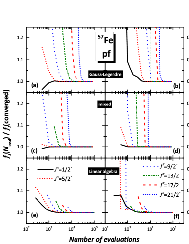
Figure 1: (Color online) Convergence, as a function of the number of evaluations, of projection via Gauss-Legendre quadrature (upper panels), via mixed quadrature, that is, inversion in the $\alpha,\gamma$ angles, equivalent to Fomenko projection/trapezoidal quadrature, as discussed in Section 2, and Gauss-Legendre quadrature on $\beta$ (middle panels), and via linear algebra (lower panels) of the fractional occupation $f_{J}$ (left panels) and the yrast energies (right panels) for ⁵⁷Fe in the $0f$-$1p$ space.

We remind the reader that our criterion for efficiency is the number of evaluations at different Euler angles required for a converged result (i.e., does not change with increased number of evaluations), and that evaluation of the norm (overlap) kernel is computationally much cheaper than for the Hamiltonian kernel. With that in mind, we broadly found that projection by linear algebra requires significantly fewer evaluations than quadrature. Furthermore, we found that convergence of the norm kernel, represented by the fractional occupation $f_{J}$, tracks the convergence of the Hamiltonian kernel and the resulting energies.

This we illustrate with three nuclides in different model spaces with different semi-phenomenological interactions in Figs. 1, 3, and 4, showing the convergence of $f_{J}$ and the yrast energies as a function of the number of evaluations, $N_{\mathrm{eval}}$. Specifically, we show the ratio $f_{J}(N_{\mathrm{eval}})/f_{J}(\mathrm{converged})$ in the left-hand panels, and the difference in the yrast energies $E^{J}(N_{\mathrm{eval}})-E^{J}(\mathrm{converged})$ in the right-hand panels. In Fig. 4 we also show the convergence of $J^{2}$, which we obtained by replacing the Hamiltonian matrix elements with those of $J^{2}$.

Figure 2: (Color online) Low-lying levels of ⁵⁷Fe in the $0f$-$1p$ space, comparing experimental and full configuration-interaction (CI) calculations with results from projected Hartree-Fock (PHF).

Our specific examples are: Fig. 1, ⁵⁷Fe in the $0f$-$1p$ shell with frozen ⁴⁰Ca core and the monopole-modified $G$-matrix interaction GX1A [35]; Fig. 3, ⁶⁸Ga in the $0f_{5/2}$-$1p$-$0g_{9/2}$ space with a frozen ⁵⁶Ni core, and the interaction JUN45 [36]; and finally Fig. 4, ⁴⁸Cr in the $1s$-$0d$-$0f$-$1p$ shells with frozen ¹⁶O core, with the interaction of [37]. Results for other nuclides are similar and not sensitive to the model space; for example, results for ⁴⁸Cr in $0f$-$1p$ shell are qualitatively indistinguishable from Fig. 4. Calculations with other nuclides, in these spaces and others, behave in very similar fashion. This includes preliminary results in even larger, multi-shell spaces.

We also show, in Fig. 2, the low-lying levels of ⁵⁷Fe from experiment [38], from full configuration-interaction shell model calculations, and using projected Hartree-Fock, with the latter two both using GX1A in the $pf$ space. In general we find projected Hartree-Fock does well in reproducing spectra of even-even nuclei, especially those which are strong rotors, poorly for odd-odd nuclei, and mixed quality for odd-$A$ nuclei. ⁵⁷Fe happens to be reasonably well-reproduced, and we speculate this may be due to being a simple particle plus rotor. In general one would want to go to configuration-mixing via, for example, the generator-coordinate method [18, 19, 20, 21, 22, 23, 24, 25]. Our purpose here is primarily to investigate the convergence of the projection method.

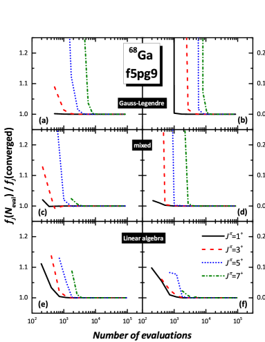
Figure 3: (Color online) Convergence, as a function of the number of evaluations, of projection via Gauss-Legendre quadrature (upper panels), via mixed quadrature, that is, inversion in the $\alpha,\gamma$ angles, equivalent to Fomenko projection/trapezoidal quadrature, as discussed in Section 2, and Gauss-Legendre quadrature on $\beta$ (middle panels), and via linear algebra (lower panels) of the fractional occupation $f_{J}$ (left panels) and the yrast energies (right panels) for ⁶⁸Ga in the $0f_{5/2}$-$1p$-$0g_{9/2}$ space. .

In Figs. 1, 3, and 4, we show three projection methods. For projection by Gauss-Legendre quadrature, we assumed the same number of mesh points $N_{\Omega}$ for all three Euler angles, so that the number of evaluations is $N_{\Omega}^{3}$. We found $N_{\Omega}=44$ (or $N_{\mathrm{eval}}=85,184$) produced reliably converged results. Smaller values of $J$ converge faster with $N_{\Omega}$ than larger values, which makes sense: one expects the large $J$ wave functions to have more nodes in $\alpha,\beta,\gamma$. For projection by linear algebra, we increased $J_{\mathrm{max}}$ until we got no change in results; increasing $J_{\mathrm{max}}$ further made no difference. The number of evaluations is roughly $4J_{\mathrm{max}}^{3}+8J_{\mathrm{max}}^{2}$. We also show a ‘mixed’ projection, where the $\beta$-integral, for rotations about the $y$-axis, is done by Gauss-Legendre quadrature, while the $\alpha$- and $\gamma$-integrals, for rotations about the $z$ axis, is done by linear algebra inversion; as discussed in section 2 this is equivalent to so-called ‘trapezoidal’ quadrature in the literature as well as Fomenko projection [31]. In these results we did not use symmetries to reduce the number of evaluations in either method.

In Figs. 1 and 3, we oriented the plots so that, reading downward, one can see the improved convergence as one goes from full Gauss-Legendre quadrature, to mixed projection, to linear algebra inversion. For Fig. 4, we changed the orientation, so that, reading down, one can compare the convergence of the fractional occupation $f_{J}$, the yrast energies, and of $J^{2}$. The latter we treated by simply replacing the Hamiltonian with the matrix elements for $J^{2}$. One sees that all three quantities converge at similar points, although the yrast energies converge with a slightly larger number of evaluations. All our other results, not only for ⁵⁷Fe and ⁶⁸Ga but many other nuclides, exhibit qualitatively the same behavior.

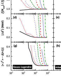
Figure 4: (Color online) Note: orientation and content differ from Figs. 1,3. Convergence, as a function of the number of evaluations, of projection via Gauss-Legendre quadrature (left-hand panels), via mixed quadrature, that is, inversion in the $\alpha,\gamma$ angles, equivalent to Fomenko discretization/trapezoidal quadrature, as discussed in Section 2, and Gauss-Legendre quadrature on $\beta$ (middle column panels), and via linear algebra (right-hand panels) of the fractional occupation $f_{J}$ (top row panels), yrast energies (middle row panels), and expectation values of $J^{2}$ (bottom row panels) for ⁴⁸Cr in the $0d$-$1s$-$0f$-$1p$ space.

Our results are summarized in Table 1, which shows the number of evaluations needed to get specific energies to within 1 keV of the converged results. This table clearly shows the advantage of projection by linear algebra, which includes for us the ‘mixed’ case of trapezoidal ‘quadrature’/Fomenko projection. For low $J$ the advantage is small, largely because in projection by quadrature one can target a specific value of $J$, say $J=0$, while in projection by linear algebra one needs to solve for all, or at least the most important (as measured by $f_{J}$) values of $J$. For larger $J$, however, projection by linear algebra robustly requires a factor of 3 fewer evaluations, or better, than pure Gauss-Legendre quadrature. Note that $J$ in Table 1 is not $J_{\mathrm{max}}$; $J_{\mathrm{max}}$ is determined by the criterion of convergence to within 1 keV.

For comparison, consider some typical number of evaluations in the literature. For projection up to $J=6$, we found reported meshes of 20,000 evaluations for mixed projection [20], and for pure Gauss-Legendre quadrature 18,000 [22] to 32,000 [10]. In a case for up to only $J=2$, Gauss-Legendre only required 3,500 evaluations [10]. It has also been reported that larger deformations, mixing in higher $J$-levels, require significantly more evaluations [22]. Note: all these calculations considered triaxially deformed but time-reversed-even states, and so used symmetries to reduce the number of actual evaluations; we multiplied by 16 in order to compare. These numbers are not too different from our values in Table 1, although we found our mixed calculations required a factor of 2 fewer evaluations to get to $J=6$.

We also experimented with our implemented need-to-know algorithm, which, by knowing that some values of $f_{J}\approx 0$, we can reduce the number of values of $\beta_{j}$ at which we need to evaluation. In some cases we could reduce the number of evaluations by a factor of two, but we found these to be rather specialized cases.

To be specific: for some even-even nuclides, the Slater determinant is time-reversal even, and only even values of $J$ are occupied (have non-zero $f_{J}$). In the $0f$-$1p$ shell, for example, both ⁴⁸Cr and ⁶⁰Fe are prolate, and we were able to reduce the number of evaluations from 12,615 to 6,728 with a change in energies by less than 0.4 keV. ⁶²Ni is oblate; using need-to-know we reduced the number of evaluations from 18,513 to 9,801, with a change in energies less than 0.6 keV. In all these cases our Monte Carlo algorithm quickly found a mesh of $\beta_{j}$ which was invertible.

We also tried need-to-know with cranked wave functions: by adding $-\omega\hat{J}_{x}$ (or any other component of angular momentum) the solution Slater determinant contains higher fractions of components at higher $J$, and smaller fractions at smaller $J$. The saving in evaluations, however, is generally small, except for large values of $\omega$. In contrast to the time-reversed even cases, with only even values of $J$, our empirical experience is that it is more difficult to find invertible meshes when deleting small values of $J$ and keeping large values; the reason remains unclear to us.

Table 1: The minimum number of evaluations needed for ⁵⁷Fe, ⁶⁸Ga, and ⁴⁸Cr when $|\Delta E^{J}|=|E^{J}(N_{\mathrm{eval}})-E^{J}(\mathrm{converged})|$ to be smaller than 1 keV. Here ‘Gauss-Legendre’ is Gaussian quadrature in all three Euler angles, ‘lin. alg.’ inverts in all three Euler angles, and ‘mixed’ means inversion in the $\alpha,\gamma$ angles, equivalent to Fomenko discretization/trapezoidal quadrature, as discussed in Section 2, with Gauss-Legendre quadrature in the $\beta$ angle.

Nuclide	$J^{\pi}$	$N_{\mathrm{eval}}$
		($|\Delta E^{J}|<1$ keV)
		Gauss-Legendre	mixed	lin. alg.
57Fe	$1/2^{+}$	5832	1000	4000
	$5/2^{+}$	8000	1728	4000
	$9/2^{+}$	13824	2744	5324
	$13/2^{+}$	13824	5832	5324
	$17/2^{+}$	27000	8000	8788
	$21/2^{+}$	32768	10648	13500
68Ga	$1^{+}$	1728	1000	1800
	$3^{+}$	5832	1728	1800
	$5^{+}$	10648	2744	2601
	$7^{+}$	13824	4096	3610
48Cr	$0^{+}$	13824	5832	8125
	$2^{+}$	13824	5832	8125
	$4^{+}$	13824	8000	8125
	$6^{+}$	21952	10648	8125
	$8^{+}$	46656	17576	12615
	$10^{+}$	64000	21952	12615
	$12^{+}$	85184	32768	18513

5 Conclusions and acknowledgements.

We have investigated two related approaches for projection of good angular momentum, projection by quadrature and projection by linear algebra. In both methods one samples matrix elements on a mesh of Euler angles; because evaluation of Hamiltonian matrix elements, is computationally expensive we want to use a minimal mesh. In particular we investigated the convergence of $f_{J}$, the fraction of the wave function with angular momentum $J$, because the sum of $f_{J}$ must be 1, and because it is cheaper to compute overlaps than energies. Therefore $f_{J}$ is our suggested key criterion for convergence, for both methods.

The situation is somewhat complicated by the fact that many papers cite a trapezoidal ‘quadrature’ method. Although justification for this method is hard to find in the literature, in our analysis this method is equivalent to our linear algebra inversion, as well as to the Fomenko projection cited in particle-number projection based upon an exact finite Fourier sum rule [31, 32]. In all cases, however, using linear algebra inversion methods, including trapezoidal ‘quadrature’ / Fomenko projection, dramatically reduce the number of evaluations required; If one is interested in projecting out states with all or most values of $J$, the reduction is as much as three-fold, i.e., only as third as many evaluations are required over Gauss-Legendre quadrature.

In all methods one can reduce the number of evaluations by using discrete symmetries. Because we do not impose axial symmetry upon our Hartree-Fock solutions, we only considered symmetries in the Euler angles $\alpha,\gamma$ (rotations about the $z$-axis). We found meshes which met the symmetry but still lead to invertible matrices. If one imposed axial symmetry, there are additional possible savings, which we did not explore.

In some cases it is possible to get additional gains by eliminating unoccupied values of $J$ and to reduce simultaneously the number of evaluations on the Euler angle $\beta$ (rotation about the $y$-axis). Aside from time-reversed-even cases, however, the gains were generally not large.

This material is based upon work supported by the U.S. Department of Energy, Office of Science, Office of Nuclear Physics, under Award Number DE-FG02-03ER41272. We are grateful to the anonymous referee who nudged us towards Fomenko projection, which led us a better understanding of the literature.

References

- [1] Peter Ring and Peter Schuck. The nuclear many-body problem. Springer Science & Business Media, 2004.
- [2] Jouni Suhonen. From Nucleons to Nucleus: Concepts of Microscopic Nuclear Theory. Springer Science & Business Media, 2007.
- [3] Aage Bohr and Ben R Mottelson. Nuclear structure, volume 2. World Scientific, 1998.
- [4] M. R. Gunye and Chindhu S. Warke. Projected hartree-fock spectra of -shell nuclei. Phys. Rev., 156:1087–1093, Apr 1967.
- [5] Tomás R. Rodríguez, J. L. Egido, L. M. Robledo, and R. Rodríguez-Guzmán. Quality of the restricted variation after projection method with angular momentum projection. Phys. Rev. C, 71:044313, Apr 2005.
- [6] K Hara, A Hayashi, and P Ring. Exact angular momentum projection of cranked hartree-fock-bogoliubov wave functions. Nuclear Physics A, 385(1):14–28, 1982.
- [7] K. Enami, K. Tanabe, and N. Yoshinaga. Microscopic description of high-spin states: Quantum-number projections of the cranked hartree-fock-bogoliubov self-consistent solution. Phys. Rev. C, 59:135–153, Jan 1999.
- [8] Javid A Sheikh and Peter Ring. Symmetry-projected hartree–fock–bogoliubov equations. Nuclear Physics A, 665(1):71–91, 2000.
- [9] M. Borrajo and J. L. Egido. A symmetry-conserving description of odd nuclei with the gogny force. The European Physical Journal A, 52(9):277, Sep 2016.
- [10] J. M. Yao, J. Meng, P. Ring, and D. Pena Arteaga. Three-dimensional angular momentum projection in relativistic mean-field theory. Phys. Rev. C, 79:044312, Apr 2009.
- [11] Michio Honma, Takahiro Mizusaki, and Takaharu Otsuka. Nuclear shell model by the quantum monte carlo diagonalization method. Phys. Rev. Lett., 77:3315–3318, Oct 1996.
- [12] T Abe, P Maris, T Otsuka, N Shimizu, Y Tsunoda, Y Utsuno, JP Vary, and T Yoshida. Recent development of monte carlo shell model and its application to no-core calculations. In Journal of Physics: Conference Series, volume 454, page 012066. IOP Publishing, 2013.
- [13] Kenji Hara and Yang Sun. Projected shell model and high-spin spectroscopy. International Journal of Modern Physics E, 4(04):637–785, 1995.
- [14] Yang Sun and Kenji Hara. Fortran code of the projected shell model: feasible shell model calculations for heavy nuclei. Computer physics communications, 104(1):245–258, 1997.
- [15] J. A. Sheikh and K. Hara. Triaxial projected shell model approach. Phys. Rev. Lett., 82:3968–3971, May 1999.
- [16] Zao-Chun Gao and Mihai Horoi. Angular momentum projected configuration interaction with realistic hamiltonians. Phys. Rev. C, 79:014311, Jan 2009.
- [17] KW Schmid. On the use of general symmetry-projected hartree–fock–bogoliubov configurations in variational approaches to the nuclear many-body problem. Progress in Particle and Nuclear Physics, 52(2):565–633, 2004.
- [18] R. Rodríguez-Guzmán, J. L. Egido, and L. M. Robledo. Quadrupole collectivity in nuclei with the angular momentum projected generator coordinate method. Phys. Rev. C, 65:024304, Jan 2002.
- [19] T. Nikšić, D. Vretenar, and P. Ring. Beyond the relativistic mean-field approximation. ii. configuration mixing of mean-field wave functions projected on angular momentum and particle number. Phys. Rev. C, 74:064309, Dec 2006.
- [20] Michael Bender and Paul-Henri Heenen. Configuration mixing of angular-momentum and particle-number projected triaxial hartree-fock-bogoliubov states using the skyrme energy density functional. Phys. Rev. C, 78:024309, Aug 2008.
- [21] J. M. Yao, J. Meng, P. Ring, and D. Vretenar. Configuration mixing of angular-momentum-projected triaxial relativistic mean-field wave functions. Phys. Rev. C, 81:044311, Apr 2010.
- [22] Tomás R. Rodríguez and J. Luis Egido. Triaxial angular momentum projection and configuration mixing calculations with the gogny force. Phys. Rev. C, 81:064323, Jun 2010.
- [23] J. M. Yao, H. Mei, H. Chen, J. Meng, P. Ring, and D. Vretenar. Configuration mixing of angular-momentum-projected triaxial relativistic mean-field wave functions. ii. microscopic analysis of low-lying states in magnesium isotopes. Phys. Rev. C, 83:014308, Jan 2011.
- [24] Marta Borrajo, Tomás R Rodríguez, and J Luis Egido. Symmetry conserving configuration mixing method with cranked states. Physics Letters B, 746:341–346, 2015.
- [25] Tomás R. Rodríguez. Precise description of nuclear spectra with gogny energy density functional methods. The European Physical Journal A, 52(7):190, Jul 2016.
- [26] Per-Olov Löwdin. Angular momentum wavefunctions constructed by projector operators. Rev. Mod. Phys., 36:966–976, Oct 1964.
- [27] Nazakat Ullah. New method for the angular-momentum projection. Phys. Rev. Lett., 27:439–442, Aug 1971.
- [28] Feng Pan, Bo Li, Yao-Zhong Zhang, and Jerry P. Draayer. Heine-stieltjes correspondence and a new angular momentum projection for many-particle systems. Phys. Rev. C, 88:034305, Sep 2013.
- [29] Calvin W. Johnson and Kevin D. O’Mara. Projection of angular momentum via linear algebra. Phys. Rev. C, 96:064304, Dec 2017.
- [30] Alan Robert Edmonds. Angular momentum in quantum mechanics. Princeton University Press, 1996.
- [31] V. N. Fomenko. Projection in the occupation-number space and the canonical transformation. Journal of Physics A: General Physics, 3(1):8, 1970.
- [32] W. E. Ormand, D. J. Dean, C. W. Johnson, G. H. Lang, and S. E. Koonin. Demonstration of the auxiliary-field monte carlo approach for sd-shell nuclei. Phys. Rev. C, 49:1422–1427, Mar 1994.
- [33] J. Dobaczewski, M. V. Stoitsov, W. Nazarewicz, and P.-G. Reinhard. Particle-number projection and the density functional theory. Phys. Rev. C, 76:054315, Nov 2007.
- [34] Ionel Stetcu and Calvin W. Johnson. Random phase approximation vs exact shell-model correlation energies. Phys. Rev. C, 66:034301, Sep 2002.
- [35] M Honma, T Otsuka, BA Brown, and T Mizusaki. Shell-model description of neutron-rich pf-shell nuclei with a new effective interaction gxpf 1. Eur. Phys. J. A, 25(1):499–502, 2005.
- [36] M. Honma, T. Otsuka, T. Mizusaki, and M. Hjorth-Jensen. New effective interaction for -shell nuclei. Phys. Rev. C, 80:064323, Dec 2009.
- [37] Y. Iwata, N. Shimizu, T. Otsuka, Y. Utsuno, J. Menéndez, M. Honma, and T. Abe. Large-scale shell-model analysis of the neutrinoless decay of . Phys. Rev. Lett., 116:112502, Mar 2016.
- [38] National nuclear data center. http://www.nndc.bnl.gov, October 2018.