The past and future dynamics of quintom dark energy models

Genly Leon genly.leon@ucn.cl Departamento de Matemáticas, Universidad Católica del Norte, Avda. Angamos 0610, Casilla 1280 Antofagasta, Chile    Andronikos Paliathanasis anpaliat@phys.uoa.gr Instituto de Ciencias Físicas y Matemáticas, Universidad Austral de Chile, Valdivia, Chile Department of Mathematics and Natural Sciences, Core Curriculum Program, Prince Mohammad Bin Fahd University, Al Khobar 31952, Kingdom of Saudi Arabia Institute of Systems Science, Durban University of Technology, PO Box 1334, Durban 4000, South Africa    Jorge Luis Morales-Martínez jorge.morales@cimat.mx Dpto. de Geomática e Hidráulica, División de Ingeniería, Universidad de Guanajuato, Guanajuato, México
Abstract

We study the phase space of the quintom cosmologies for a class of exponential potentials. We combine normal forms expansions and the center manifold theory in order to describe the dynamics near equilibrium sets. Furthermore, we construct the unstable and center manifold of the massless scalar field cosmology motivated by the numerical results given in Lazkoz and Leon (Phys Lett B 638:303. arXiv:astro-ph/0602590, 2006). We study the role of the curvature on the dynamics. Several monotonic functions are defined on relevant invariant sets for the quintom cosmology. Finally, conservation laws of the cosmological field equations and algebraic solutions are determined by using the symmetry analysis and the singularity analysis.

I Introduction

Recent observations coming from type I-a Supernovae (SNIa), large scale structure (LSS) formation, and the cosmic microwave background (CMBR) Radiation 1 ; 2 ; 3 ; 4 ; 5 ; 6 ; 7 ; 8 ; 9 ; 10 ; 11 ; 12 ; 13 ; 14 ; 15 ; 16 , indicates the universe is expanding with an accelerated rate without been settled until now a definitive model to account for this phenomena. One of the current alternatives models for such acceleration of the expansion is the yet unknown form of matter named dark energy. Several models of dark energy use a single scalar field, e.g., the so called phantom field and the quintessence field 17 ; 18 . Furthermore, one can consider models with two fields, in particular combining quintessence and phantom fields one can built up the so-called quintom models 19 ; 20 ; 21 ; 22 ; 23 ; 24 ; 25 ; 26 ; 27 ; 28 ; 29 ; 30 ; 31 ; 32 ; 33 ; 34 ; 35 ; 36 ; 37 ; 38 ; 39 ; 40 ; 41 ; 42 ; 43 ; 44 ; 45 . These models admits the crossing of the boundary w=1𝑤1w=-1 with w𝑤w being the equation of state parameter of the cosmic fluid. This behavior has been investigated in several cosmological theories, for example: h-essence cosmologies28 ; 29 ; holographic dark energy 46 ; 47 ; 48 ; 49 ; inspired by string theory 33 ; by considering spinor matter 37 ; 38 ; for arbitrary potentials 40 ; 41 ; 42 ; 43 ; 44 ; using isomorphic models consisting of coupled oscillators 50 ; Pais–Uhlenbeck oscillator 51 ; inspired in scalar tensor theories 52 ; 53 ; 54 ; 55 ; 56 as well as in modified theories of gravity 57 ; 58 . Furthermore, interacting quintom in nonminimal coupling has been studied in 59 , and quintom with nonminimal derivative coupling was studied in 60 . An extension of the quintom scenario, in which the scalar fields are coupled through a kinetic interaction, have been studied in 61 ; 62 while an interacting quintom model was recently constructed by the application of the generalized uncertainty principle (GUP) in the scalar field Lagrangian [63]. In particular, the second scalar field of the quintom model in 63 corresponds to higher-order derivatives given by the GUP. Furthermore, one of the particularly exciting solutions of quintom type models is that they can provide a classically stable bouncing solution. This was first pointed out in 61 and two important extensions were made in 62 and 63 , which discussed the Lee-Wick and Horndeski realizations, respectively. The cosmology of the quintom model with exponential potentials was investigated in 30 and 31 ; 32 . More specifically, 31 ; 32 the potential accounts for the interaction between the conventional scalar field and the phantom field. In contrary with 30 where no such interaction was assumed. In 31 was found that the interaction term dominates over the mixed terms of the potential.This simplification has important consequences such that the existence of scaling attractors excludes the existence of phantom attractors, as a difference with the results in 32 . Some of these results were extended in 40 , for arbitrary potentials. In the recent years still there an special interest in this kind of models with the phantom crossing behavior 67 ; 68 ; 69 ; 70 ; 71 ; 72 ; 73 . In line with this interest, we stress in this paper a deep insight about the model proposed in 31 . The plan of the paper it follows. In Section II we make a general description of the model under study and we present the field equations. In Section II.1 are presented several monotonic functions defined on invariant sets of the phase space using the results summarized in the Appendix A. The equilibrium points of the model for any curvature choice using H𝐻H-normalization are discussed in Section II.2. In Section II.2.1 we make the analysis of zero-curvature models with two scalar fields, one a linear function of the other. Furthermore, in section II.3 we present some improvements of the results from reference 31 . In particular, in Section II.3.1 we discuss the normal expansion with undetermined coefficients of arbitrary order that is used to construct the unstable and center manifold up to fourth order in Leon:2008aq for flat FRW metric. We explicitly state in the Appendix B the main techniques to use, following the approach of arrowsmith ; wiggins ; wiggins2 . In section II.4 we introduce an alternative of the variables used in 31 for flat FRW models that renders the phase space in compact form. In this new variables we find static universe configurations that cannot by discussed in the framework of 31 . This illustrates the applicability of this formulation in compact variables. Moreover, in Section III we propose several normalization procedures for investigating models with flat and non flat spatial curvature, that allows to circumvent some technical problems that arises, for example when the crossing through H=0𝐻0H=0, where H𝐻H is the Hubble factor, happens. The integrability of the quintom cosmological model is studied in Section IV. In particular we apply two different methods to determine the integrability, the symmetry analysis and the singularity analysis. Finally, in Section V we discuss our results and draw our conclusions.

II The quintom model

In this work we consider the so-called two-field quintom with Lagrangian 31 :

=12μϕμϕ12μψμψV(ϕ,ψ),12subscript𝜇italic-ϕsuperscript𝜇italic-ϕ12subscript𝜇𝜓superscript𝜇𝜓𝑉italic-ϕ𝜓\displaystyle\mathcal{L}=\frac{1}{2}\partial_{\mu}\phi\partial^{\mu}\phi-\frac{1}{2}\partial_{\mu}\psi\partial^{\mu}\psi-V(\phi,\psi), (1)
V(ϕ,ψ)=V0e6(mϕ+nψ),𝑉italic-ϕ𝜓subscript𝑉0superscript𝑒6𝑚italic-ϕ𝑛𝜓\displaystyle V(\phi,\psi)=V_{0}e^{-\sqrt{6}(m\phi+n\psi)}, (2)

where the scalar field ϕitalic-ϕ\phi represents quintessence and ψ𝜓\psi represents a phantom field, and we include a co-moving perfect fluid in the gravitational action. We use the Friedmann-Robertson-Walker (FRW) line element given in spherical coordinates by:

ds2=dt2+a(t)2(dr21kr2+r2dθ2+r2sin2θdϑ2).𝑑superscript𝑠2𝑑superscript𝑡2𝑎superscript𝑡2dsuperscript𝑟21𝑘superscript𝑟2superscript𝑟2dsuperscript𝜃2superscript𝑟2superscript2𝜃dsuperscriptitalic-ϑ2ds^{2}=-dt^{2}+a(t)^{2}\left(\frac{\mathrm{d}r^{2}}{1-kr^{2}}+r^{2}\mathrm{d}\theta^{2}+r^{2}\sin^{2}\theta\mathrm{d}\vartheta^{2}\right). (3)

The scalar curvature of the 3-metric induced on the space-like surfaces orthogonal to 𝐞0=tsubscript𝐞0subscript𝑡{\bf e}_{0}=\partial_{t} is given by R3=6ka2,k=1,0,1,formulae-sequencesuperscript𝑅36𝑘superscript𝑎2𝑘101{}^{3}\!R=\frac{6k}{a^{2}},\quad k=1,0,-1, where k𝑘k identifies the three types of FRW universes: closed, flat, and open, respectively.

The field equations derived for the line element (3) in the context of General Relativity, are given by

H216(ϕ˙2ψ˙2)13V(ϕ,ψ)13ρ=R36,superscript𝐻216superscript˙italic-ϕ2superscript˙𝜓213𝑉italic-ϕ𝜓13𝜌superscript𝑅36\displaystyle H^{2}-{\textstyle{1\over 6}}\left(\dot{\phi}^{2}-\dot{\psi}^{2}\right)-{\textstyle{1\over 3}}V(\phi,\psi)-{\textstyle{1\over 3}}\rho=-{\textstyle{{}^{3}\!R\over 6}},
H˙=H213(ϕ˙2ψ˙2)+13V(ϕ,ψ)16(3γ2)ρ,˙𝐻superscript𝐻213superscript˙italic-ϕ2superscript˙𝜓213𝑉italic-ϕ𝜓163𝛾2𝜌\displaystyle\dot{H}=-H^{2}-{\textstyle{1\over 3}}\left(\dot{\phi}^{2}-\dot{\psi}^{2}\right)+{\textstyle{1\over 3}}V(\phi,\psi)-{\textstyle{1\over 6}}(3\gamma-2)\rho,
ρ˙=3γHρ,˙𝜌3𝛾𝐻𝜌\displaystyle\dot{\rho}=-3\gamma H\rho,
ϕ¨+3Hϕ˙6mV(ϕ,ψ)=0,¨italic-ϕ3𝐻˙italic-ϕ6𝑚𝑉italic-ϕ𝜓0\displaystyle\ddot{\phi}+3H\dot{\phi}-\sqrt{6}mV(\phi,\psi)=0,
ψ¨+3Hψ˙+6nV(ϕ,ψ)=0,¨𝜓3𝐻˙𝜓6𝑛𝑉italic-ϕ𝜓0\displaystyle\ddot{\psi}+3H\dot{\psi}+\sqrt{6}nV(\phi,\psi)=0, (4)

where H=a˙(t)a(t)𝐻˙𝑎𝑡𝑎𝑡H=\frac{\dot{a}(t)}{a(t)} denotes the Hubble function, while the dot denotes differentiation with respect to variable t𝑡t. Moreover, the barotropic index of the background matter, γ,𝛾\gamma, is assumed to take values on the interval 0<γ<2.0𝛾20<\gamma<2.

For the stability analysis of cosmological models one can apply linearization around fixed points, Monotonic Principle LeBlanc:1994qm , the Invariant Manifold Theorem reza ; arrowsmith ; wiggins ; wiggins2 ; aulbach , the Center Manifold Theorem arrowsmith ; carr ; wiggins ; wiggins2 , and Normal Forms (NF) theory arrowsmith ; wiggins ; wiggins2 .

Introducing the following normalized variables

xϕ=ϕ˙6H,xψ=ψ˙6H,y=V3H,z=ρ3H,formulae-sequencesubscript𝑥italic-ϕ˙italic-ϕ6𝐻formulae-sequencesubscript𝑥𝜓˙𝜓6𝐻formulae-sequence𝑦𝑉3𝐻𝑧𝜌3𝐻x_{\phi}=\frac{\dot{\phi}}{\sqrt{6}H},\;x_{\psi}=\frac{\dot{\psi}}{\sqrt{6}H},\;y=\frac{\sqrt{V}}{\sqrt{3}H},\;z=\frac{\sqrt{\rho}}{\sqrt{3}H}, (5)

the Friedmann equation becomes

1+xϕ2xψ2+y2+z2=R36H2,1superscriptsubscript𝑥italic-ϕ2superscriptsubscript𝑥𝜓2superscript𝑦2superscript𝑧2superscript𝑅36superscript𝐻2-1+x_{\phi}^{2}-x_{\psi}^{2}+y^{2}+z^{2}={\textstyle{{}^{3}\!R\over 6H^{2}}}, (6)

and the deceleration factor qa¨a/a˙2𝑞¨𝑎𝑎superscript˙𝑎2q\equiv-\ddot{a}a/\dot{a}^{2} can be expressed in terms of the new variables as

q=12(3γ2)z2+2(xϕ2xψ2)y2.𝑞123𝛾2superscript𝑧22superscriptsubscript𝑥italic-ϕ2superscriptsubscript𝑥𝜓2superscript𝑦2q={\textstyle{1\over 2}}(3\gamma-2)z^{2}+2\left(x_{\phi}^{2}-x_{\psi}^{2}\right)-y^{2}. (7)

The new variables (5) can be used to rewrite the system (4) as a system of first-order ordinary differential equations (ODEs):

xϕ=13(3my2+(q2)xϕ),superscriptsubscript𝑥italic-ϕ133𝑚superscript𝑦2𝑞2subscript𝑥italic-ϕ\displaystyle x_{\phi}^{\prime}={\textstyle{1\over 3}}\left(3my^{2}+(q-2)x_{\phi}\right), (8)
xψ=13(3ny2(q2)xψ),superscriptsubscript𝑥𝜓133𝑛superscript𝑦2𝑞2subscript𝑥𝜓\displaystyle x_{\psi}^{\prime}=-{\textstyle{1\over 3}}\left(3ny^{2}-(q-2)x_{\psi}\right), (9)
y=13(1+q3(mxϕ+nxψ))y,superscript𝑦131𝑞3𝑚subscript𝑥italic-ϕ𝑛subscript𝑥𝜓𝑦\displaystyle y^{\prime}={\textstyle{1\over 3}}(1+q-3(mx_{\phi}+nx_{\psi}))y, (10)
z=16(1+2q3γ)z,superscript𝑧1612𝑞3𝛾𝑧\displaystyle z^{\prime}={\textstyle{1\over 6}}(1+2q-3\gamma)z, (11)

where the primes denote derivative with respect to τ=loga3.𝜏superscript𝑎3\tau=\log a^{3}.

II.1 Invariant set and monotonic functions

By following the procedures in the Appendix A, we can find the invariant sets.

Remark 1.

The sets {𝐱4|xϕ2xψ2+y2+z21}conditional-set𝐱superscript4less-than-or-equals-or-greater-thansuperscriptsubscript𝑥italic-ϕ2superscriptsubscript𝑥𝜓2superscript𝑦2superscript𝑧21\left\{\mathbf{x}\in\mathbb{R}^{4}|x_{\phi}^{2}-x_{\psi}^{2}+y^{2}+z^{2}\lesseqqgtr 1\right\}, {𝐱4|nxϕ+mxψ0}conditional-set𝐱superscript4less-than-or-equals-or-greater-than𝑛subscript𝑥italic-ϕ𝑚subscript𝑥𝜓0\left\{\mathbf{x}\in\mathbb{R}^{4}|nx_{\phi}+mx_{\psi}\lesseqqgtr 0\right\}, {𝐱4|y0}conditional-set𝐱superscript4less-than-or-equals-or-greater-than𝑦0\left\{\mathbf{x}\in\mathbb{R}^{4}|y\lesseqqgtr 0\right\}, and {𝐱4|z0}conditional-set𝐱superscript4less-than-or-equals-or-greater-than𝑧0\left\{\mathbf{x}\in\mathbb{R}^{4}|z\lesseqqgtr 0\right\} are invariant sets of (8-11).

By using the equations ddτln(1+xϕ2xψ2+y2+z2)=23q𝑑𝑑𝜏1superscriptsubscript𝑥italic-ϕ2superscriptsubscript𝑥𝜓2superscript𝑦2superscript𝑧223𝑞\frac{d}{d\tau}\ln(-1+x_{\phi}^{2}-x_{\psi}^{2}+y^{2}+z^{2})=\frac{2}{3}q, and ddτln(nxϕ+mxψ)=13(q2)𝑑𝑑𝜏𝑛subscript𝑥italic-ϕ𝑚subscript𝑥𝜓13𝑞2\frac{d}{d\tau}\ln(nx_{\phi}+mx_{\psi})=\frac{1}{3}(q-2), it follows from Proposition 10 that the sign of R3superscript𝑅3{}^{3}\!R and the sign of nxϕ+mxψ𝑛subscript𝑥italic-ϕ𝑚subscript𝑥𝜓nx_{\phi}+mx_{\psi} are invariant. From equations (8-11) it is obvious that any combination of signs for y𝑦y and z𝑧z is an invariant set for the flow.

Remark 2.

For R3=0superscript𝑅30{}^{3}\!R=0, {𝐱3|xϕ2xψ2+y21}conditional-set𝐱superscript3superscriptsubscript𝑥italic-ϕ2superscriptsubscript𝑥𝜓2superscript𝑦21\left\{\mathbf{x}\in\mathbb{R}^{3}|x_{\phi}^{2}-x_{\psi}^{2}+y^{2}\leqq 1\right\} are invariant sets of the flow of (8-11).

Defining on this sets the function Z=xϕ2xψ2+y21𝑍superscriptsubscript𝑥italic-ϕ2superscriptsubscript𝑥𝜓2superscript𝑦21Z=x_{\phi}^{2}-x_{\psi}^{2}+y^{2}-1 that has directional derivative along the flow given by Z=αZsuperscript𝑍𝛼𝑍Z^{\prime}=\alpha Z where α𝛼\alpha is a continuous real-valued non-vanishing function on 3superscript3\mathbb{R}^{3} given by α=xϕ2xψ2y2𝛼superscriptsubscript𝑥italic-ϕ2superscriptsubscript𝑥𝜓2superscript𝑦2\alpha=x_{\phi}^{2}-x_{\psi}^{2}-y^{2}. Hence, by applying Proposition 10, the desired result follows. In the same way it is proved that y=0𝑦0y=0 is an invariant set of the flow by defining α=1+q3(mxϕ+nxψ)𝛼1𝑞3𝑚subscript𝑥italic-ϕ𝑛subscript𝑥𝜓\alpha=1+q-3\left(mx_{\phi}+nx_{\psi}\right). Combining the former results we can prove that the 2-dimensional set Γ={𝐱3:0<xϕ2xψ2<1,y=0}Γconditional-set𝐱superscript3formulae-sequence0superscriptsubscript𝑥italic-ϕ2superscriptsubscript𝑥𝜓21𝑦0\Gamma=\left\{\mathbf{x}\in\mathbb{R}^{3}:0<x_{\phi}^{2}-x_{\psi}^{2}<1,y=0\right\} is invariant under the flow. Notice that the equilibrium points O𝑂O and C±subscript𝐶plus-or-minusC_{\pm} studied in 31 are in the boundary of ΓΓ\Gamma.

Below: Φ(𝐱0,t)Φsubscript𝐱0𝑡\Phi({\bf x}_{0},t) is the unique solution of the system satisfying Φ(𝐱0,0)=𝐱0Φsubscript𝐱00subscript𝐱0\Phi({\bf x}_{0},0)={\bf x}_{0}; O(𝐱0)𝑂subscript𝐱0O({\bf x}_{0}) denotes the unique orbit passing through 𝐱0subscript𝐱0{\bf x}_{0}; α(𝐱0)𝛼subscript𝐱0\alpha({\bf x}_{0}) means the past attractor or α𝛼\alpha-limit of 𝐱0subscript𝐱0{\bf x}_{0}, defined by α(𝐱0)={𝐲:{tn}n1,tn,limn+Φ(𝐱0,tn)=𝐲}𝛼subscript𝐱0conditional-set𝐲formulae-sequencesubscriptsubscript𝑡𝑛𝑛1subscript𝑡𝑛subscript𝑛Φsubscript𝐱0subscript𝑡𝑛𝐲\alpha({\bf x}_{0})=\{{\bf y}:\exists\{t_{n}\}_{n\geq 1},t_{n}\rightarrow-\infty,\lim_{n\rightarrow+\infty}\Phi({\bf x}_{0},t_{n})={\bf y}\}; and ω(𝐱0)𝜔subscript𝐱0\omega({\bf x}_{0}) means the future attractor or ω𝜔\omega-limit of 𝐱0subscript𝐱0{\bf x}_{0}, defined by ω(𝐱0)={𝐲:{tn}n1,tn+,limn+Φ(𝐱0,tn)=𝐲}𝜔subscript𝐱0conditional-set𝐲formulae-sequencesubscriptsubscript𝑡𝑛𝑛1subscript𝑡𝑛subscript𝑛Φsubscript𝐱0subscript𝑡𝑛𝐲\omega({\bf x}_{0})=\{{\bf y}:\exists\{t_{n}\}_{n\geq 1},t_{n}\rightarrow+\infty,\lim_{n\rightarrow+\infty}\Phi({\bf x}_{0},t_{n})={\bf y}\}.

Proposition 1.

Let 𝐱0S1:={𝐱:nxϕ+mxψ0,xϕ2xψ2+y2+z21}subscript𝐱0subscript𝑆1assignconditional-set𝐱formulae-sequence𝑛subscript𝑥italic-ϕ𝑚subscript𝑥𝜓0superscriptsubscript𝑥italic-ϕ2superscriptsubscript𝑥𝜓2superscript𝑦2superscript𝑧21{\bf x}_{0}\in S_{1}:=\{{\bf x}:nx_{\phi}+mx_{\psi}\neq 0,x_{\phi}^{2}-x_{\psi}^{2}+y^{2}+z^{2}\neq 1\} such that O(𝐱0)𝑂subscript𝐱0O({\bf x}_{0}) is bounded. Then, α(𝐱0){𝐱:xϕ2xψ2+y2+z2=1}𝛼subscript𝐱0conditional-set𝐱superscriptsubscript𝑥italic-ϕ2superscriptsubscript𝑥𝜓2superscript𝑦2superscript𝑧21\alpha({\bf x}_{0})\subset\{{\bf x}:x_{\phi}^{2}-x_{\psi}^{2}+y^{2}+z^{2}=1\} and ω(𝐱0){𝐱:nxϕ+mxψ=0}.𝜔subscript𝐱0conditional-set𝐱𝑛subscript𝑥italic-ϕ𝑚subscript𝑥𝜓0\omega({\bf x}_{0})\subset\{{\bf x}:nx_{\phi}+mx_{\psi}=0\}.

Proof. Let W1=(nxϕ+mxψ)4(xϕ2xψ2+y2+z21)2,W1=83W1.formulae-sequencesubscript𝑊1superscript𝑛subscript𝑥italic-ϕ𝑚subscript𝑥𝜓4superscriptsubscript𝑥italic-ϕ2superscriptsubscript𝑥𝜓2superscript𝑦2superscript𝑧212superscriptsubscript𝑊183subscript𝑊1W_{1}=\frac{\left(nx_{\phi}+mx_{\psi}\right)^{4}}{\left(x_{\phi}^{2}-x_{\psi}^{2}+y^{2}+z^{2}-1\right){2}},W_{1}^{\prime}=-{\textstyle{8\over 3}}W_{1}. Thus, W1subscript𝑊1W_{1} is positive and strictly monotone along orbits of the invariant set S1subscript𝑆1S_{1}. The boundary of S1subscript𝑆1S_{1} is the invariant set S1¯S1={𝐱:nxϕ+mxψ=0}{𝐱:xϕ2xψ2+y2+z2=1}¯subscript𝑆1subscript𝑆1conditional-set𝐱𝑛subscript𝑥italic-ϕ𝑚subscript𝑥𝜓0conditional-set𝐱superscriptsubscript𝑥italic-ϕ2superscriptsubscript𝑥𝜓2superscript𝑦2superscript𝑧21\bar{S_{1}}\setminus S_{1}=\{{\bf x}:nx_{\phi}+mx_{\psi}=0\}\cup\{{\bf x}:x_{\phi}^{2}-x_{\psi}^{2}+y^{2}+z^{2}=1\}. Let be any initial state 𝐱0S1subscript𝐱0subscript𝑆1{\bf x}_{0}\in S_{1} such that O(𝐱0)𝑂subscript𝐱0O({\bf x}_{0}) remains bounded. Therefore, a:=inf𝐱S1W1(𝐱)=0assign𝑎subscriptinfimum𝐱subscript𝑆1subscript𝑊1𝐱0a:=\inf_{{\bf x}\in S_{1}}W_{1}({\bf x})=0 is attained at {𝐱:nxϕ+mxψ=0}conditional-set𝐱𝑛subscript𝑥italic-ϕ𝑚subscript𝑥𝜓0\{{\bf x}:nx_{\phi}+mx_{\psi}=0\} and b:=sup𝐱S1W1(𝐱)=assign𝑏subscriptsupremum𝐱subscript𝑆1subscript𝑊1𝐱b:=\sup_{{\bf x}\in S_{1}}W_{1}({\bf x})=\infty is attained at {𝐱:xϕ2xψ2+y2+z2=1}conditional-set𝐱superscriptsubscript𝑥italic-ϕ2superscriptsubscript𝑥𝜓2superscript𝑦2superscript𝑧21\{{\bf x}:x_{\phi}^{2}-x_{\psi}^{2}+y^{2}+z^{2}=1\}. By the Monotonicity Principle (Theorem 1), α(𝐱0){𝐱:xϕ2xψ2+y2+z2=1}𝛼subscript𝐱0conditional-set𝐱superscriptsubscript𝑥italic-ϕ2superscriptsubscript𝑥𝜓2superscript𝑦2superscript𝑧21\alpha({\bf x}_{0})\subset\{{\bf x}:x_{\phi}^{2}-x_{\psi}^{2}+y^{2}+z^{2}=1\}, ω(𝐱0){𝐱:nxϕ+mxψ=0}.𝜔subscript𝐱0conditional-set𝐱𝑛subscript𝑥italic-ϕ𝑚subscript𝑥𝜓0\omega({\bf x}_{0})\subset\{{\bf x}:nx_{\phi}+mx_{\psi}=0\}. \blacksquare

Proposition 2.

Consider 𝐱0S2:={𝐱:z>0,nxϕ+mxψ0}subscript𝐱0subscript𝑆2assignconditional-set𝐱formulae-sequence𝑧0𝑛subscript𝑥italic-ϕ𝑚subscript𝑥𝜓0{\bf x}_{0}\in S_{2}:=\{{\bf x}:z>0,\;nx_{\phi}+mx_{\psi}\neq 0\} such that O(𝐱0)𝑂subscript𝐱0O({\bf x}_{0}) is bounded. Then α(𝐱0){𝐱:z=0}𝛼subscript𝐱0conditional-set𝐱𝑧0\alpha({\bf x}_{0})\subset\{{\bf x}:z=0\} and ω(𝐱0){𝐱:nxϕ+mxψ=0}.𝜔subscript𝐱0conditional-set𝐱𝑛subscript𝑥italic-ϕ𝑚subscript𝑥𝜓0\omega({\bf x}_{0})\subset\{{\bf x}:nx_{\phi}+mx_{\psi}=0\}.

Proof. Let W2=(nxϕ+mxψ)2z2,W2=(γ2)W2.formulae-sequencesubscript𝑊2superscript𝑛subscript𝑥italic-ϕ𝑚subscript𝑥𝜓2superscript𝑧2superscriptsubscript𝑊2𝛾2subscript𝑊2W_{2}=\frac{\left(nx_{\phi}+mx_{\psi}\right)^{2}}{z^{2}},W_{2}^{\prime}=(\gamma-2)W_{2}. Thus, W2subscript𝑊2W_{2} is positive and strictly monotone along orbits of the invariant set S2subscript𝑆2S_{2}. Hence, the boundary of S2subscript𝑆2S_{2} is the invariant set S2¯S2={𝐱:nxϕ+mxψ=0}{𝐱:z=0}¯subscript𝑆2subscript𝑆2conditional-set𝐱𝑛subscript𝑥italic-ϕ𝑚subscript𝑥𝜓0conditional-set𝐱𝑧0\bar{S_{2}}\setminus S_{2}=\{{\bf x}:nx_{\phi}+mx_{\psi}=0\}\cup\{{\bf x}:z=0\}. Let be any initial state 𝐱0S1subscript𝐱0subscript𝑆1{\bf x}_{0}\in S_{1} such that O(𝐱0)𝑂subscript𝐱0O({\bf x}_{0}) remains bounded. By Theorem 1, α(𝐱0){𝐱:z=0}𝛼subscript𝐱0conditional-set𝐱𝑧0\alpha({\bf x}_{0})\subset\{{\bf x}:z=0\}, ω(𝐱0){𝐱:nxϕ+mxψ=0}.𝜔subscript𝐱0conditional-set𝐱𝑛subscript𝑥italic-ϕ𝑚subscript𝑥𝜓0\omega({\bf x}_{0})\subset\{{\bf x}:nx_{\phi}+mx_{\psi}=0\}. \blacksquare

Proposition 3.

Let 𝐱0S3:={𝐱:xϕ2xψ2+y2+z21,z>0}subscript𝐱0subscript𝑆3assignconditional-set𝐱formulae-sequencesuperscriptsubscript𝑥italic-ϕ2superscriptsubscript𝑥𝜓2superscript𝑦2superscript𝑧21𝑧0{\bf x}_{0}\in S_{3}:=\{{\bf x}:x_{\phi}^{2}-x_{\psi}^{2}+y^{2}+z^{2}\neq 1,\;z>0\} such that O(𝐱0)𝑂subscript𝐱0O({\bf x}_{0}) is bounded. Then:

  • if γ>23𝛾23\gamma>{\textstyle{2\over 3}}, α(𝐱0){𝐱:xϕ2xψ2+y2+z2=1}𝛼subscript𝐱0conditional-set𝐱superscriptsubscript𝑥italic-ϕ2superscriptsubscript𝑥𝜓2superscript𝑦2superscript𝑧21\alpha({\bf x}_{0})\subset\{{\bf x}:x_{\phi}^{2}-x_{\psi}^{2}+y^{2}+z^{2}=1\} and ω(𝐱0){𝐱:z=0}𝜔subscript𝐱0conditional-set𝐱𝑧0\omega({\bf x}_{0})\subset\{{\bf x}:z=0\}.

  • if γ<23𝛾23\gamma<{\textstyle{2\over 3}}, α(𝐱0){𝐱:z=0}𝛼subscript𝐱0conditional-set𝐱𝑧0\alpha({\bf x}_{0})\subset\{{\bf x}:z=0\} and ω(𝐱0){𝐱:xϕ2xψ2+y2+z2=1}𝜔subscript𝐱0conditional-set𝐱superscriptsubscript𝑥italic-ϕ2superscriptsubscript𝑥𝜓2superscript𝑦2superscript𝑧21\omega({\bf x}_{0})\subset\{{\bf x}:x_{\phi}^{2}-x_{\psi}^{2}+y^{2}+z^{2}=1\}.

Proof. Let W3=z4(xϕ2xψ2+y2+z21)2,W3=23(3γ2)W3.formulae-sequencesubscript𝑊3superscript𝑧4superscriptsuperscriptsubscript𝑥italic-ϕ2superscriptsubscript𝑥𝜓2superscript𝑦2superscript𝑧212superscriptsubscript𝑊3233𝛾2subscript𝑊3W_{3}=\frac{z^{4}}{\left(x_{\phi}^{2}-x_{\psi}^{2}+y^{2}+z^{2}-1\right)^{2}},W_{3}^{\prime}=-{\textstyle{2\over 3}}(3\gamma-2)W_{3}. W3subscript𝑊3W_{3} is positive monotonic decreasing (increasing) in the invariant set S3subscript𝑆3S_{3} for non-zero curvature models provided γ>23𝛾23\gamma>{\textstyle{2\over 3}} (γ<23𝛾23\gamma<{\textstyle{2\over 3}}). S3¯S3={𝐱:z=0}{𝐱:xϕ2xψ2+y2+z2=1}¯subscript𝑆3subscript𝑆3conditional-set𝐱𝑧0conditional-set𝐱superscriptsubscript𝑥italic-ϕ2superscriptsubscript𝑥𝜓2superscript𝑦2superscript𝑧21\bar{S_{3}}\setminus S_{3}=\{{\bf x}:z=0\}\cup\{{\bf x}:x_{\phi}^{2}-x_{\psi}^{2}+y^{2}+z^{2}=1\}. Let be 𝐱0S3subscript𝐱0subscript𝑆3{\bf x}_{0}\in S_{3} such that O(𝐱0)𝑂subscript𝐱0O({\bf x}_{0}) is bounded. By Theorem 1 we conclude. \blacksquare

Proposition 4.

Let 𝐱0S4:={(xϕ,xψ,y):0<xϕ2xψ2<1,y=0}subscript𝐱0subscript𝑆4assignconditional-setsubscript𝑥italic-ϕsubscript𝑥𝜓𝑦formulae-sequence0superscriptsubscript𝑥italic-ϕ2superscriptsubscript𝑥𝜓21𝑦0{\bf x}_{0}\in S_{4}:=\left\{(x_{\phi},\,x_{\psi},y):0<x_{\phi}^{2}-x_{\psi}^{2}<1,y=0\right\}, such that O(𝐱0)𝑂subscript𝐱0O({\bf x}_{0}) is bounded. Then, α(𝐱0)C:={𝐱:xϕ2xψ2=1}𝛼subscript𝐱0𝐶assignconditional-set𝐱superscriptsubscript𝑥italic-ϕ2superscriptsubscript𝑥𝜓21\alpha({\bf x}_{0})\subset C:=\{{\bf x}:x_{\phi}^{2}-x_{\psi}^{2}=1\} and ω(𝐱0){𝐱:nxϕ+mxψ=0}.𝜔subscript𝐱0conditional-set𝐱𝑛subscript𝑥italic-ϕ𝑚subscript𝑥𝜓0\omega({\bf x}_{0})\subset\{{\bf x}:nx_{\phi}+mx_{\psi}=0\}.

Proof. Let be W4=(nxϕ+mxψ)4(1xϕ2+xψ2)2,W4=4(q2)3(1xϕ2+xψ2)W4.formulae-sequencesubscript𝑊4superscript𝑛subscript𝑥italic-ϕ𝑚subscript𝑥𝜓4superscript1superscriptsubscript𝑥italic-ϕ2superscriptsubscript𝑥𝜓22superscriptsubscript𝑊44𝑞231superscriptsubscript𝑥italic-ϕ2superscriptsubscript𝑥𝜓2subscript𝑊4W_{4}=\frac{(nx_{\phi}+mx_{\psi})^{4}}{(1-x_{\phi}^{2}+x_{\psi}^{2})^{2}},W_{4}^{\prime}=\frac{4(q-2)}{3(1-x_{\phi}^{2}+x_{\psi}^{2})}W_{4}. Notice q=12(3(xϕ2xψ2)+1)<2𝑞123superscriptsubscript𝑥italic-ϕ2superscriptsubscript𝑥𝜓212q={\textstyle{1\over 2}}\left(3(x_{\phi}^{2}-x_{\psi}^{2})+1\right)<2 since y=0𝑦0y=0 and 0<xϕ2xψ2<1.0superscriptsubscript𝑥italic-ϕ2superscriptsubscript𝑥𝜓210<x_{\phi}^{2}-x_{\psi}^{2}<1. Then, W4subscript𝑊4W_{4} is positive and strictly monotone along orbits of the invariant set S4subscript𝑆4S_{4}. S4¯S4={𝐱:nxϕ+mxψ=0}{𝐱:xϕ2xψ2=1}¯subscript𝑆4subscript𝑆4conditional-set𝐱𝑛subscript𝑥italic-ϕ𝑚subscript𝑥𝜓0conditional-set𝐱superscriptsubscript𝑥italic-ϕ2superscriptsubscript𝑥𝜓21\bar{S_{4}}\setminus S_{4}=\{{\bf x}:nx_{\phi}+mx_{\psi}=0\}\cup\{{\bf x}:x_{\phi}^{2}-x_{\psi}^{2}=1\}. Let be any initial state 𝐱0S4subscript𝐱0subscript𝑆4{\bf x}_{0}\in S_{4} such that O(𝐱0)𝑂subscript𝐱0O({\bf x}_{0}) remains bounded. By Theorem 1 we find α(𝐱0)C:={𝐱:xϕ2xψ2=1}𝛼subscript𝐱0𝐶assignconditional-set𝐱superscriptsubscript𝑥italic-ϕ2superscriptsubscript𝑥𝜓21\alpha({\bf x}_{0})\subset C:=\{{\bf x}:x_{\phi}^{2}-x_{\psi}^{2}=1\} and ω(𝐱0){𝐱:nxϕ+mxψ=0}.𝜔subscript𝐱0conditional-set𝐱𝑛subscript𝑥italic-ϕ𝑚subscript𝑥𝜓0\omega({\bf x}_{0})\subset\{{\bf x}:nx_{\phi}+mx_{\psi}=0\}. \blacksquare

Remark 3.

In 31 it was devised the monotonic function W5=xϕ4(1xϕ2+xψ2)2,W5=2W5,formulae-sequencesubscript𝑊5superscriptsubscript𝑥italic-ϕ4superscript1superscriptsubscript𝑥italic-ϕ2superscriptsubscript𝑥𝜓22superscriptsubscript𝑊52subscript𝑊5W_{5}=\frac{x_{\phi}^{4}}{(1-x_{\phi}^{2}+x_{\psi}^{2})^{2}},{W_{5}}^{\prime}=-2{W_{5}}, defined in the invariant set of zero-curvature models with dust matter. There it was argued that the orbits initially near the hyperbolas (representing massless scalar field cosmologies) tends asymptotically to the flat FRW universe. On the other hand, from the monotonic function W4subscript𝑊4W_{4} we can conclude that (for zero-curvature models) the orbits which initially near the hyperbolas tends asymptotically to either the matter scaling (MS) solutions (equilibrium points like T𝑇T) or (in the absence of scaling solutions) to powerlaw solutions (equilibrium points like P𝑃P).

Remark 4.

The previous gallery of monotonic functions can be used to ruled out, according to Proposition 11, the existence of homoclinic orbits, recurrent orbits and more complex behavior in several invariant sets. The dynamics is dominated by equilibrium points and heteroclinic orbits joining it. Therefore, some global results can be found from the linear (local) analysis of equilibrium points.

II.2 The equilibrium points

The system (8-11) admits six types of equilibrium points (with both z𝑧z and y𝑦y non-negative) denoted by M,F,C±,P,MS,𝑀𝐹subscript𝐶plus-or-minus𝑃𝑀𝑆M,\;F,\;C_{\pm},\;P,\;MS, and CS.𝐶𝑆CS. In tables 1 and 2 we offer some partial information of these equilibrium points like the location, conditions for existence, dynamical character and some additional information. For zero-curvature models (with dust background, i.e., γ=1𝛾1\gamma=1), the equilibrium point MS𝑀𝑆MS and P𝑃P reduces respectively to the points T𝑇T and P,𝑃P, investigated in 31 .

The equilibrium point M𝑀M represents the Milne universe, it has negative curvature. It is no hyperbolic if γ=23.𝛾23\gamma={\textstyle{2\over 3}}. F𝐹F denotes the flat FRW universe and it is no hyperbolic if γ=23𝛾23\gamma={\textstyle{2\over 3}} or γ=2.𝛾2\gamma=2. For γ<2/3𝛾23\gamma<2/3 (resp. γ>2/3𝛾23\gamma>2/3) the eigenvalues of M𝑀M (resp. F𝐹F) are (,,+,+)(-,-,+,+) and the eigenvalues of F𝐹F (resp. M𝑀M) are (,,+,)(-,-,+,-). In this case both equilibrium points act locally as saddles. The 3-dimensional stable subspace of F𝐹F (resp. M𝑀M) intersects the 2-dimensional unstable subspace of M𝑀M (resp. F𝐹F) at the z𝑧z axis. This means that the orbits initially at this axis are asymptotic to the past to the Milne (resp. flat FRW) universe and to the flat FRW (resp. Milne) universe toward the future.

The equilibrium sets given by the hyperbolas C±subscript𝐶plus-or-minusC_{\pm} were investigated in 31 , the same analysis done in that reference is valid in our more general context. In the former section we conjecture that they are local sources for the quintom phase-space. In fact, if δ>1𝛿1\delta>1 then part of the hyperbola is a local attractor to the past, and part of it is a saddle. If δ<1𝛿1\delta<1 then the entire hyperbola is a local attractor to the past.

The equilibrium point P𝑃P denotes a zero-curvature power-law inflationary model if δ<1/3𝛿13\delta<1/3, corresponding to the equilibrium point with the same label investigated in 31 . It is worth noticing that the results of 31 concerning to this equilibrium point applies here only in the case of zero-curvature models with a dust background. It is non hyperbolic if δ=13𝛿13\delta={\textstyle{1\over 3}} or δ=γ2.𝛿𝛾2\delta={\textstyle{\gamma\over 2}}. P𝑃P is a local inflationary attractor if either 0<γ<2/3,δ<γ/2formulae-sequence0𝛾23𝛿𝛾20<\gamma<2/3,\;\delta<\gamma/2 or 2/3<γ<2,δ<1/3.formulae-sequence23𝛾2𝛿132/3<\gamma<2,\;\delta<1/3. If 2/3<γ<223𝛾22/3<\gamma<2 and 1/3<δ<γ/213𝛿𝛾21/3<\delta<\gamma/2 then it is no longer a local inflationary solution nor an attractor for non-zero curvature models. However in this case the eigenvalues are (+,,,)(+,-,-,-) and then, the equilibrium point has a 3-dimensional stable subspace. If 0<γ<2/30𝛾230<\gamma<2/3 and γ/2<δ<1/3𝛾2𝛿13\gamma/2<\delta<1/3 the eigenvalues of P𝑃P are (,,,+).(-,-,-,+). Hence, although an inflationary solution, P𝑃P is not longer a local attractor. In this case the stable subspace is 3-dimensional.

The equilibrium point MS𝑀𝑆MS represents a matter scaling model. It is no hyperbolic if γ=0𝛾0\gamma=0 or γ=2/3𝛾23\gamma={2}/{3} or γ=2.𝛾2\gamma=2. If 2/3<γ<223𝛾22/3<\gamma<2 the eigenvalues are (,+,,).(-,+,-,-). In this case the equilibrium point behaves like a saddle, the stable subspace being 3-dimensional. Otherwise the equilibrium point is stable. If either 0<γ2/9,δ>γ/2formulae-sequence0𝛾29𝛿𝛾20<\gamma\leq{2}/{9},\;\delta>{\gamma}/{2} or if 2/9<γ2/3,γ/2<δ4γ2/(9γ2)formulae-sequence29𝛾23𝛾2𝛿4superscript𝛾29𝛾2{2}/{9}<\gamma\leq{2}/{3},\;{\gamma}/{2}<\delta\leq{4\gamma^{2}}/{(9\gamma-2)}, the equilibrium point behaves as an stable node. If 2/9<γ<2/3,δ>4γ2/(9γ2)formulae-sequence29𝛾23𝛿4superscript𝛾29𝛾2{2}/{9}<\gamma<{2}/{3},\;\delta>{4\gamma^{2}}/{(9\gamma-2)} there are two complex eigenvalues and the orbits spiral-in toward MS𝑀𝑆MS in a 2-dimensional subspace.

As stated in 31 , point P𝑃P is the local attractor for zero-curvature models provided there are not scaling regimes. As we have seen, for some region in the parameters space the equilibrium points P𝑃P and MS𝑀𝑆MS exist in the same phase portrait with P𝑃P having eigenvalues (,,,+)(-,-,-,+) (i.e, a saddle) and MS𝑀𝑆MS being a local attractor (i.e., all its eigenvalues having positive real part). If 0<γ2/3, 1/3<δ<1formulae-sequence0𝛾2313𝛿10<\gamma\leq 2/3,\;1/3<\delta<1 or 2/3<γ<2,γ/2<δ<1formulae-sequence23𝛾2𝛾2𝛿12/3<\gamma<2,\;\gamma/2<\delta<1 the eigenvalues of P𝑃P are (+,,,+).(+,-,-,+). In the latter case, the stable subspace of P𝑃P is 2 dimensional and then it is the local attractor for zero-curvature models without matter.

Furthermore, the equilibrium point CS𝐶𝑆CS denotes curvature scaling models. It is no hyperbolic if γ=2/3𝛾23\gamma={2}/{3} or δ=3/7.𝛿37\delta={3}/{7}. It is stable if 2/3<γ<2,δ>3/7,formulae-sequence23𝛾2𝛿37{2}/{3}<\gamma<2,\;\delta>{3}/{7}, and then, with negative curvature. If 2/3<γ<2, 3/7<δ4/9,formulae-sequence23𝛾237𝛿49{2}/{3}<\gamma<2,\;{3}/{7}<\delta\leq{4}/{9}, then the eigenvalues are negative real and CS𝐶𝑆CS behaves as a stable node. If 2/3<γ<2,δ>4/9formulae-sequence23𝛾2𝛿49{2}/{3}<\gamma<2,\;\delta>{4}/{9} the orbits spiral-in toward CS𝐶𝑆CS in a 2-dimensional subspace (since in this case two eigenvalues are complex conjugated). Otherwise, CS𝐶𝑆CS is unstable. Its stable subspace is 3-dimensional if either γ>2/3, 0<δ<3/7formulae-sequence𝛾23 0𝛿37\gamma>2/3,\;0<\delta<3/7 or 0<γ<2/3, 3/7<δ4/9formulae-sequence0𝛾2337𝛿490<\gamma<2/3,\;3/7<\delta\leq 4/9. This subspace is 2-dimensional if 0<γ<2/3, 0<δ<3/7.formulae-sequence0𝛾23 0𝛿370<\gamma<2/3,\;0<\delta<3/7.

II.2.1 A flat FRW model with one scalar field a linear function of the other

Consider the 2-dimensional invariant set nxϕ+mxψ=0,xϕ2xψ2+y2+z2=1formulae-sequence𝑛subscript𝑥italic-ϕ𝑚subscript𝑥𝜓0superscriptsubscript𝑥italic-ϕ2superscriptsubscript𝑥𝜓2superscript𝑦2superscript𝑧21nx_{\phi}+mx_{\psi}=0,x_{\phi}^{2}-x_{\psi}^{2}+y^{2}+z^{2}=1. Let m0𝑚0m\neq 0 such that xψ=nxϕ/msubscript𝑥𝜓𝑛subscript𝑥italic-ϕ𝑚x_{\psi}=-nx_{\phi}/m. Therefore, (1n2m2)xϕ2+y2+z2=11superscript𝑛2superscript𝑚2superscriptsubscript𝑥italic-ϕ2superscript𝑦2superscript𝑧21\left(1-\frac{n^{2}}{m^{2}}\right)x_{\phi}^{2}+y^{2}+z^{2}=1. The dynamics is governed by the equations:

xϕsuperscriptsubscript𝑥italic-ϕ\displaystyle x_{\phi}^{\prime} =(1γ2)xϕ((1n2m2)xϕ21)+(mγ2xϕ)y2,absent1𝛾2subscript𝑥italic-ϕ1superscript𝑛2superscript𝑚2superscriptsubscript𝑥italic-ϕ21𝑚𝛾2subscript𝑥italic-ϕsuperscript𝑦2\displaystyle=\left(1-{\textstyle{\gamma\over 2}}\right)x_{\phi}\left(\left(1-{\textstyle{n^{2}\over m^{2}}}\right)x_{\phi}^{2}-1\right)+\left(m-{\textstyle{\gamma\over 2}}x_{\phi}\right)y^{2}, (12)
ysuperscript𝑦\displaystyle y^{\prime} =12y[xϕ(2m+xϕ(γ2))(1n2m2)+(y21)γ],absent12𝑦delimited-[]subscript𝑥italic-ϕ2𝑚subscript𝑥italic-ϕ𝛾21superscript𝑛2superscript𝑚2superscript𝑦21𝛾\displaystyle=-\frac{1}{2}y\Big{[}x_{\phi}(2m+x_{\phi}(\gamma-2))\left(1-{\textstyle{n^{2}\over m^{2}}}\right)+\left(y^{2}-1\right)\gamma\Big{]}, (13)

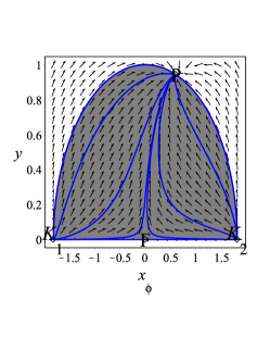
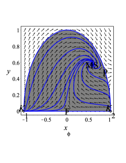
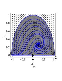
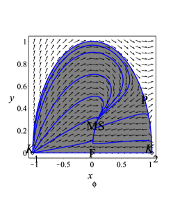
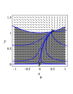
defined on the phase plane: Ψ={(xϕ,y):0(1n2m2)xϕ2+y21,y0}.Ψconditional-setsubscript𝑥italic-ϕ𝑦formulae-sequence01superscript𝑛2superscript𝑚2superscriptsubscript𝑥italic-ϕ2superscript𝑦21𝑦0\Psi=\left\{(x_{\phi},y):0\leq\left(1-\frac{n^{2}}{m^{2}}\right)x_{\phi}^{2}+y^{2}\leq 1,\;y\geq 0\right\}. We have two cases: Case i) if m2n2,superscript𝑚2superscript𝑛2m^{2}\geq n^{2}, the phase plane ΨΨ\Psi is the half of the ellipse 0(1n2/m2)xϕ2+y2101superscript𝑛2superscript𝑚2superscriptsubscript𝑥italic-ϕ2superscript𝑦210\leq(1-{n^{2}}/{m^{2}})x_{\phi}^{2}+y^{2}\leq 1. Case ii) if m2<n2,superscript𝑚2superscript𝑛2m^{2}<n^{2}, the phase space is half of the hyperbola 0(1n2/m2)xϕ2+y21.01superscript𝑛2superscript𝑚2superscriptsubscript𝑥italic-ϕ2superscript𝑦210\leq(1-{n^{2}}/{m^{2}})x_{\phi}^{2}+y^{2}\leq 1. The conditions for existence and the dynamical behavior of the equilibrium points are presented in Table 3.

In figure 1 it is shown some orbits of the system (12)-(13) for (a) m=0.6,n=0.5,γ=1formulae-sequence𝑚0.6formulae-sequence𝑛0.5𝛾1m=0.6,n=0.5,\gamma=1, (b) m=0.9,n=0.2,γ=1formulae-sequence𝑚0.9formulae-sequence𝑛0.2𝛾1m=0.9,n=0.2,\gamma=1, (c) m=2.0,n=0.5,γ=1formulae-sequence𝑚2.0formulae-sequence𝑛0.5𝛾1m=2.0,n=0.5,\gamma=1, (d) m=0.9,n=0.2,γ=0.1formulae-sequence𝑚0.9formulae-sequence𝑛0.2𝛾0.1m=0.9,n=0.2,\gamma=0.1 and (e) m=0.5,n=0.6,γ=1formulae-sequence𝑚0.5formulae-sequence𝑛0.6𝛾1m=0.5,n=0.6,\gamma=1. The shadowed region represents the physical portion of the phase plane which is either half ellipse or half hyperbola.

Label (xϕ,xψ,y,z)subscript𝑥italic-ϕsubscript𝑥𝜓𝑦𝑧(x_{\phi},x_{\psi},y,z) Existence Deceleration q𝑞q Curvature Solution
M𝑀M (0,0,0,0)0000(0,0,0,0) All m𝑚m and n𝑛n q=0𝑞0q=0 R3<0superscript𝑅30{}^{3}\!R<0 Milne
F𝐹F (0,0,0,1)0001(0,0,0,1) All m𝑚m and n𝑛n q=1+3γ2𝑞13𝛾2q=-1+\frac{3\gamma}{2} R3=0superscript𝑅30{}^{3}\!R=0 Flat FRW
C±subscript𝐶plus-or-minusC_{\pm} (±1+xψ2,xψ,0,0)plus-or-minus1superscriptsuperscriptsubscript𝑥𝜓2superscriptsubscript𝑥𝜓00\left(\pm\sqrt{1+{x_{\psi}^{*}}^{2}},x_{\psi}^{*},0,0\right) All m𝑚m and n𝑛n q=2𝑞2q=2 R3=0superscript𝑅30{}^{3}\!R=0 Massless Scalar Field
P𝑃{P} (m,n,1δ,0)𝑚𝑛1𝛿0(m,-n,\sqrt{1-\delta},0) δ<1𝛿1\delta<1 q=1+3δ𝑞13𝛿q=-1+3\delta R3=0superscript𝑅30{}^{3}\!R=0 Powerlaw
MS𝑀𝑆{MS} (mγ2δ,nγ2δ,(2γ)γ2δ,1γ2δ)𝑚𝛾2𝛿𝑛𝛾2𝛿2𝛾𝛾2𝛿1𝛾2𝛿\left(\displaystyle\frac{\displaystyle m\gamma}{\displaystyle 2\delta},-\displaystyle\frac{\displaystyle n\gamma}{\displaystyle 2\delta},\displaystyle\frac{\sqrt{(2-\gamma)\gamma}}{2\sqrt{\delta}},\displaystyle\sqrt{1-\displaystyle\frac{\displaystyle\gamma}{\displaystyle 2\delta}}\right) δ>γ2𝛿𝛾2\delta>\displaystyle\frac{\displaystyle\gamma}{\displaystyle 2} q=1+3γ2𝑞13𝛾2q=-1+\frac{3\gamma}{2} R3=0superscript𝑅30{}^{3}\!R=0 Matter Scaling
CS𝐶𝑆{CS} (m3δ,n3δ,23δ,0)𝑚3𝛿𝑛3𝛿23𝛿0\left(\displaystyle\frac{\displaystyle m}{\displaystyle 3\delta},-\displaystyle\frac{\displaystyle n}{\displaystyle 3\delta},\displaystyle\frac{\sqrt{2}}{3\sqrt{\delta}},0\right) δ>0𝛿0\delta>0 q=0𝑞0q=0 R3{<0ifδ>13=0ifδ=13>0if 0<δ<13superscript𝑅3casesabsent0if𝛿13absent0if𝛿13absent0if 0𝛿13{}^{3}\!R\;\left\{\begin{array}[]{cc}<0&\text{if}\;\delta>{\textstyle{1\over 3}}\\[5.69046pt] =0&\text{if}\;\delta={\textstyle{1\over 3}}\\[5.69046pt] >0&\text{if}\;0<\delta<{\textstyle{1\over 3}}\\[5.69046pt] \end{array}\right. Curvature Scaling
Table 1: Location, existence and some properties of the equilibrium points of the system (8), (9), (10) and (11) for z0𝑧0z\geq 0, and y0.𝑦0y\geq 0. We use the notation δ=m2n2.𝛿superscript𝑚2superscript𝑛2\delta=m^{2}-n^{2}.
Name Eigenvalues Dynamical character
M𝑀M (23,23,13,16(23γ))2323131623𝛾\displaystyle\left(-{\textstyle{2\over 3}},-{\textstyle{2\over 3}},{\textstyle{1\over 3}},{\textstyle{1\over 6}}(2-3\gamma)\right) no hyperbolic if γ=23;𝛾23\gamma={\textstyle{2\over 3}}; unstable otherwise
F𝐹F (1+γ2,1+γ2,γ2,13(23γ))1𝛾21𝛾2𝛾21323𝛾\displaystyle\left(-1+{\textstyle{\gamma\over 2}},-1+{\textstyle{\gamma\over 2}},{\textstyle{\gamma\over 2}},-{\textstyle{1\over 3}}(2-3\gamma)\right) no hyperbolic if γ=23𝛾23\gamma={\textstyle{2\over 3}} or γ=2;𝛾2\gamma=2; unstable otherwise
C±subscript𝐶plus-or-minusC_{\pm} (0,43,1γ2,1nxψm1+xψ2)0431𝛾2minus-or-plus1𝑛superscriptsubscript𝑥𝜓𝑚1superscriptsuperscriptsubscript𝑥𝜓2\displaystyle\left(0,{\textstyle{4\over 3}},1-{\textstyle{\gamma\over 2}},1-nx_{\psi}^{*}\mp m\sqrt{1+{x_{\psi}^{*}}^{2}}\right) no hyperbolic
P𝑃{P} (23+2δ,1+δ,1+δ,γ2+δ)232𝛿1𝛿1𝛿𝛾2𝛿\left(-{\textstyle{2\over 3}}+2\delta,-1+\delta,-1+\delta,-{\textstyle{\gamma\over 2}}+\delta\right) no hyperbolic if δ=13𝛿13\delta={\textstyle{1\over 3}} or δ=γ2;𝛿𝛾2\delta={\textstyle{\gamma\over 2}};
stable if 0<γ230𝛾23\displaystyle 0<\gamma\leq{\textstyle{2\over 3}} and δ<γ2𝛿𝛾2\displaystyle\delta<{\textstyle{\gamma\over 2}}, or 23<γ<223𝛾2\displaystyle{\textstyle{2\over 3}}<\gamma<2 and δ<13;𝛿13\displaystyle\delta<{\textstyle{1\over 3}};
unstable otherwise
MS𝑀𝑆{MS} (1+γ2,23+γ,14(2+γ±(2γ)(29γ+4γ2δ)))1𝛾223𝛾14plus-or-minus2𝛾2𝛾29𝛾4superscript𝛾2𝛿\left(\displaystyle-1+\frac{\gamma}{2},-\displaystyle\frac{2}{3}+\gamma,\displaystyle\frac{1}{4}\left(-2+\gamma\pm\sqrt{(2-\gamma)\left(2-9\gamma+\frac{4\gamma^{2}}{\delta}\right)}\right)\right) non hyperbolic if γ=0𝛾0\gamma=0 or γ=23𝛾23\gamma={\textstyle{2\over 3}} or γ=2;𝛾2\gamma=2;
unstable (saddle) if 23<γ<2;23𝛾2\frac{2}{3}<\gamma<2; stable otherwise.
CS𝐶𝑆{CS} (23,16(23γ),13±43δ3)231623𝛾plus-or-minus1343𝛿3\left(\displaystyle-\frac{2}{3},\displaystyle\frac{1}{6}(2-3\gamma),-\displaystyle\frac{1}{3}\pm\sqrt{\frac{4}{3\delta}-3}\right) non hyperbolic if γ=23𝛾23\gamma={\textstyle{2\over 3}} or δ=37;𝛿37\delta={\textstyle{3\over 7}};
stable when 23<γ<2,δ>37;formulae-sequence23𝛾2𝛿37\frac{2}{3}<\gamma<2,\;\delta>\frac{3}{7}; unstable otherwise.
Table 2: Eigenvalues, and dynamical character of the fixed points of the system (8), (9), (10) and (11) for y0𝑦0y\geq 0 and z0.𝑧0z\geq 0.
(y,xϕ)𝑦subscript𝑥italic-ϕ(y,x_{\phi}) Existence Eigenvalues Dynamical character
Case i) m2n2superscript𝑚2superscript𝑛2m^{2}\geq n^{2} Case ii) m2<n2superscript𝑚2superscript𝑛2m^{2}<n^{2}
K1,2subscript𝐾12K_{1,2} (0,mδ)0minus-or-plus𝑚𝛿\left(0,\mp\frac{m}{\sqrt{\delta}}\right) δ>0𝛿0\delta>0 not-exists\nexists (1δ,2γ)minus-or-plus1𝛿2𝛾\left(1\mp\sqrt{\delta},2-\gamma\right) K1::subscript𝐾1absentK_{1}: non-hyperbolic if δ=1𝛿1\delta=1
saddle if δ>1𝛿1\delta>1
source otherwise
K2::subscript𝐾2absentK_{2}: source.
F𝐹F (0,0)00(0,0) mnfor-all𝑚for-all𝑛\forall m\forall n (γ21,γ2)𝛾21𝛾2\left({\textstyle{\gamma\over 2}}-1,{\textstyle{\gamma\over 2}}\right) saddle
P𝑃P (1δ,m)1𝛿𝑚\left(\sqrt{1-\delta},m\right) δ1𝛿1\delta\leq 1 mnfor-all𝑚for-all𝑛\forall m\forall n (δ1,2δγ)𝛿12𝛿𝛾\left(\delta-1,2\delta-\gamma\right) non-hyperbolic if δ=1𝛿1\delta=1 or δ=γ2𝛿𝛾2\delta={\textstyle{\gamma\over 2}}
a sink if δ<γ2𝛿𝛾2\delta<{\textstyle{\gamma\over 2}}
saddle otherwise
MS𝑀𝑆MS (12(2γ)γδ,mγ2δ)122𝛾𝛾𝛿𝑚𝛾2𝛿\left(\frac{1}{2}\sqrt{{\textstyle{(2-\gamma)\gamma\over\delta}}},{\textstyle{m\gamma\over 2\delta}}\right) δγ2>0𝛿𝛾20\delta\geq{\textstyle{\gamma\over 2}}>0 not-exists\nexists 14(2+γ±(2γ)(29γ+4γ2δ))14plus-or-minus2𝛾2𝛾29𝛾4superscript𝛾2𝛿{\textstyle{1\over 4}}\left(-2+\gamma\pm\sqrt{(2-\gamma)(2-9\gamma+{\textstyle{4\gamma^{2}\over\delta}})}\right) non-hyperbolic if δ=γ2𝛿𝛾2\delta={\textstyle{\gamma\over 2}}
stable node if 0<γ290𝛾290<\gamma\leq{\textstyle{2\over 9}} or
if 29<γ23,δ4γ2(9γ2)formulae-sequence29𝛾23𝛿4superscript𝛾29𝛾2{\textstyle{2\over 9}}<\gamma\leq{\textstyle{2\over 3}},\delta\leq{\textstyle{4\gamma^{2}\over(9\gamma-2)}}
stable spiral if
29<γ<2,δ>4γ2(9γ2)formulae-sequence29𝛾2𝛿4superscript𝛾29𝛾2{\textstyle{2\over 9}}<\gamma<2,\delta>{\textstyle{4\gamma^{2}\over(9\gamma-2)}}
Table 3: The equilibrium points of the system (19)-(20). We use the notation δ=m2n2.𝛿superscript𝑚2superscript𝑛2\delta=m^{2}-n^{2}. It is assumed 0<γ<20𝛾20<\gamma<2.
Refer to caption
(a)   m=0.6,n=0.5,γ=1formulae-sequence𝑚0.6formulae-sequence𝑛0.5𝛾1m=0.6,n=0.5,\gamma=1.
Refer to caption
(b)   m=0.9,n=0.2,γ=1formulae-sequence𝑚0.9formulae-sequence𝑛0.2𝛾1m=0.9,n=0.2,\gamma=1.
Refer to caption
(c)   m=2,n=0.5,γ=1formulae-sequence𝑚2formulae-sequence𝑛0.5𝛾1m=2,n=0.5,\gamma=1.
Refer to caption
(d)   m=0.9,n=0.2,γ=0.1formulae-sequence𝑚0.9formulae-sequence𝑛0.2𝛾0.1m=0.9,n=0.2,\gamma=0.1.
Refer to caption
(e)   m=0.5,n=0.6,γ=1formulae-sequence𝑚0.5formulae-sequence𝑛0.6𝛾1m=0.5,n=0.6,\gamma=1.
Figure 1: Some orbits in the phase plane of the system (12)-(13) for five choices of the parameters.
Refer to caption
(a)   m=0.5,n=0.6,γ=1formulae-sequence𝑚0.5formulae-sequence𝑛0.6𝛾1m=0.5,n=0.6,\gamma=1.
Refer to caption
(b)   m=0.6,n=0.5,γ=1formulae-sequence𝑚0.6formulae-sequence𝑛0.5𝛾1m=0.6,n=0.5,\gamma=1.
Refer to caption
(c)   m=0.2,n=0.2,γ=1formulae-sequence𝑚0.2formulae-sequence𝑛0.2𝛾1m=0.2,n=0.2,\gamma=1.
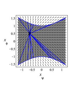
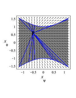
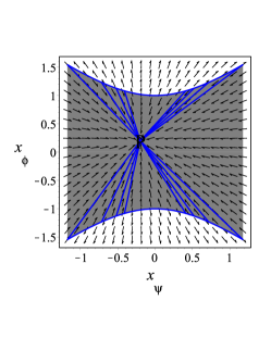
Figure 2: Some orbits in the phase plane of the system (19)-(20) for three choices of the parameters.

II.3 Flat FRW geometry and dust matter

For the flat FRW geometry and dust matter dynamics is governed by the vector field 31 :

xϕ=13(3my2+(q2)xϕ)superscriptsubscript𝑥italic-ϕ133𝑚superscript𝑦2𝑞2subscript𝑥italic-ϕ\displaystyle x_{\phi}^{\prime}=\frac{1}{3}\left(3my^{2}+(q-2)x_{\phi}\right) (14)
xψ=13(3ny2(q2)xψ)superscriptsubscript𝑥𝜓133𝑛superscript𝑦2𝑞2subscript𝑥𝜓\displaystyle x_{\psi}^{\prime}=-\frac{1}{3}\left(3ny^{2}-(q-2)x_{\psi}\right) (15)
y=13(1+q3(mxϕ+nxψ))y,superscript𝑦131𝑞3𝑚subscript𝑥italic-ϕ𝑛subscript𝑥𝜓𝑦\displaystyle y^{\prime}=\frac{1}{3}(1+q-3(mx_{\phi}+nx_{\psi}))y, (16)

where the deceleration factor is

q=12(3(xϕ2xψ2y2)+1),𝑞123superscriptsubscript𝑥italic-ϕ2superscriptsubscript𝑥𝜓2superscript𝑦21q=\frac{1}{2}\left(3\left(x_{\phi}^{2}-x_{\psi}^{2}-y^{2}\right)+1\right), (17)

defined in the phase space given by

Ψ={𝐱=(xϕ,xψ,y):0xϕ2xψ2+y21}.Ψconditional-set𝐱subscript𝑥italic-ϕsubscript𝑥𝜓𝑦0superscriptsubscript𝑥italic-ϕ2superscriptsubscript𝑥𝜓2superscript𝑦21\Psi=\{{\bf x}=(x_{\phi},x_{\psi},y):0\leq x_{\phi}^{2}-x_{\psi}^{2}+y^{2}\leq 1\}. (18)
Name xϕsubscript𝑥italic-ϕx_{\phi} xψsubscript𝑥𝜓x_{\psi} y𝑦y Existence q𝑞q
O𝑂O 00 00 00 All m𝑚m and n𝑛n 1212{\textstyle{1\over 2}}
C±subscript𝐶plus-or-minusC_{\pm} ±1+xψ2plus-or-minus1superscriptsuperscriptsubscript𝑥𝜓2\pm\sqrt{1+{x_{\psi}^{*}}^{2}} xψsuperscriptsubscript𝑥𝜓x_{\psi}^{*} 00 All m𝑚m and n𝑛n 222
P𝑃{P} m𝑚m n𝑛-n 1δ1𝛿\sqrt{1-\delta} δ<1𝛿1\delta<1 1+3δ13𝛿-1+3\delta
T𝑇{T} m2δ𝑚2𝛿\displaystyle\frac{\displaystyle m}{\displaystyle{2}{\delta}} n2δ𝑛2𝛿-\displaystyle\frac{\displaystyle n}{\displaystyle{2}{\delta}} 12δ12𝛿\displaystyle\frac{1}{2\sqrt{\delta}} δ1/2𝛿12\delta\geq 1/2 1212\displaystyle\frac{1}{2}
Table 4: Location, existence and deceleration factor of the equilibrium points for m>0𝑚0m>0, n>0𝑛0n>0 and y>0𝑦0y>0 31 .

In table 4 it is presented some information of the equilibrium points O,C±,T,P𝑂subscript𝐶plus-or-minus𝑇𝑃O,C_{\pm},T,P from 31 . We have the following cases 31 : Case i) If m<n2+1/2,𝑚superscript𝑛212m<\sqrt{n^{2}+1/2}, the point P𝑃P is an stable node and T𝑇T does not exists. Case ii) For n2+1/2<mn2+4/7,superscript𝑛212𝑚superscript𝑛247\sqrt{n^{2}+1/2}<m\leq\sqrt{n^{2}+4/7}, the point T𝑇T is a stable node and P𝑃P is a saddle point. Case iii) For n2+4/7<m<1+n2,superscript𝑛247𝑚1superscript𝑛2\sqrt{n^{2}+4/7}<m<\sqrt{1+n^{2}}, point T is a spiral node and the point P is a saddle. Case iv) For m>1+n2𝑚1superscript𝑛2m>\sqrt{1+n^{2}} the point T𝑇T is a spiral node whereas the point P𝑃P does not exist.

For R3=0,z=0formulae-sequencesuperscript𝑅30𝑧0{}^{3}\!R=0,z=0, that is, the quintom cosmological model (1) with potential (2) in the spatially flat geometry and without any other matter source, the dynamical system is reduced to

xϕ=(xϕm)(xϕ2xψ21),superscriptsubscript𝑥italic-ϕsubscript𝑥italic-ϕ𝑚superscriptsubscript𝑥italic-ϕ2superscriptsubscript𝑥𝜓21\displaystyle x_{\phi}^{\prime}=(x_{\phi}-m)\left(x_{\phi}^{2}-x_{\psi}^{2}-1\right), (19)
xψ=(n+xψ)(xϕ2xψ21),superscriptsubscript𝑥𝜓𝑛subscript𝑥𝜓superscriptsubscript𝑥italic-ϕ2superscriptsubscript𝑥𝜓21\displaystyle x_{\psi}^{\prime}=(n+x_{\psi})\left(x_{\phi}^{2}-x_{\psi}^{2}-1\right), (20)

defined on the phase plane

{(xϕ,xψ)2:xϕ2xψ21}.conditional-setsubscript𝑥italic-ϕsubscript𝑥𝜓superscript2superscriptsubscript𝑥italic-ϕ2superscriptsubscript𝑥𝜓21\{(x_{\phi},x_{\psi})\in\mathbb{R}^{2}:x_{\phi}^{2}-x_{\psi}^{2}\leq 1\}. (21)

In the figure 2 are presented some orbits in the phase plane of the system (19)-(20) for three choices of the parameters. This figures depict the typical behavior of the quintom model with exponential potential and no other matter component (vacuum quintom), where the P𝑃P is always an stable node. The shadowed region corresponds to the physical region. The region w<1𝑤1w<-1 is reached provided m2n2<0superscript𝑚2superscript𝑛20m^{2}-n^{2}<0, so the crossing does indeed occur in the case m=0.5,n=0.6formulae-sequence𝑚0.5𝑛0.6m=0.5,n=0.6 whence P𝑃P is a phantom-like solution. For m=0.6,n=0.5formulae-sequence𝑚0.6𝑛0.5m=0.6,n=0.5 the equation of state remains above w=1𝑤1w=-1 and P𝑃P is a quintessence-like solution, and for m=n=0.2𝑚𝑛0.2m=n=0.2, w=1𝑤1w=-1, such that P𝑃P represents a de Sitter solution.

Remark 5.

For R3=0,z=0formulae-sequencesuperscript𝑅30𝑧0{}^{3}\!R=0,z=0, the sets {𝐱2:mxϕ+nxψ=0}conditional-set𝐱superscript2𝑚subscript𝑥italic-ϕ𝑛subscript𝑥𝜓0\{{\bf x}\in\mathbb{R}^{2}:mx_{\phi}+nx_{\psi}=0\} and {𝐱2:xϕxψm+n1=0}conditional-set𝐱superscript2subscript𝑥italic-ϕsubscript𝑥𝜓𝑚𝑛10\{{\bf x}\in\mathbb{R}^{2}:\frac{x_{\phi}-x_{\psi}}{m+n}-1=0\} are invariant sets of the flow of (19)-(20).

Defining Ψ1=mxϕ+nxψsubscriptΨ1𝑚subscript𝑥italic-ϕ𝑛subscript𝑥𝜓\Psi_{1}=mx_{\phi}+nx_{\psi}, we show that Ψ1=Ψ1(xϕ2xψ21)superscriptsubscriptΨ1subscriptΨ1superscriptsubscript𝑥italic-ϕ2superscriptsubscript𝑥𝜓21\Psi_{1}^{\prime}=\Psi_{1}\left(x_{\phi}^{2}-x_{\psi}^{2}-1\right). Such that {𝐱:Ψ1=0}conditional-set𝐱subscriptΨ10\{{\bf x}:\Psi_{1}=0\} is an invariant set. Defining Ψ2=xϕxψm+n1subscriptΨ2subscript𝑥italic-ϕsubscript𝑥𝜓𝑚𝑛1\Psi_{2}=\frac{x_{\phi}-x_{\psi}}{m+n}-1, we show that Ψ2=Ψ2(xϕ2xψ21)superscriptsubscriptΨ2subscriptΨ2superscriptsubscript𝑥italic-ϕ2superscriptsubscript𝑥𝜓21\Psi_{2}^{\prime}=\Psi_{2}\left(x_{\phi}^{2}-x_{\psi}^{2}-1\right). Such that {𝐱:Ψ2=0}conditional-set𝐱subscriptΨ20\{{\bf x}:\Psi_{2}=0\} is an invariant set.

II.3.1 Normal expansion up to arbitrary order

In this section we obtain the normal form expansion for an arbitrary point lying on the curve Csubscript𝐶C_{-} Leon:2008aq .

Proposition 5.

Let be the vector field 𝐗𝐗{\bf X} given by (14-16) which is Csuperscript𝐶C^{\infty} in a neighborhood of 𝐱=(xϕ,xψ,y)TC.superscript𝐱superscriptsuperscriptsubscript𝑥italic-ϕsuperscriptsubscript𝑥𝜓superscript𝑦𝑇subscript𝐶{\bf x}^{*}=(x_{\phi}^{*},x_{\psi}^{*},y^{*})^{T}\in C_{-}. Let mn>0,𝑚𝑛0m\geq n>0, and xψ,superscriptsubscript𝑥𝜓x_{\psi}^{*}\in\mathbb{R}, such that λ3=1nxψ+m1+xψ2subscript𝜆31𝑛superscriptsubscript𝑥𝜓𝑚1superscriptsuperscriptsubscript𝑥𝜓2\lambda_{3}=1-nx_{\psi}^{*}+m\sqrt{1+{x_{\psi}^{*}}^{2}}\notin\mathbb{Z}, then, there exist constants ar,br,cr,r2subscript𝑎𝑟subscript𝑏𝑟subscript𝑐𝑟𝑟2a_{r},\,b_{r},\,c_{r},\;r\geq 2 (non necessarily different from zero) and a transformation of coordinates 𝐱𝐲,𝐱𝐲{\bf x}\rightarrow{\bf y}, such that (14-16) has normal form

y1superscriptsubscript𝑦1\displaystyle y_{1}^{\prime} =\displaystyle= r=2Nary1r+O(|𝐲|N+1),superscriptsubscript𝑟2𝑁subscript𝑎𝑟superscriptsubscript𝑦1𝑟𝑂superscript𝐲𝑁1\displaystyle\sum_{r=2}^{N}a_{r}y_{1}^{r}+{O}(|{\bf y}|^{N+1}), (22)
y2superscriptsubscript𝑦2\displaystyle y_{2}^{\prime} =\displaystyle= y2(1+r=2Nbry1r1)+O(|𝐲|N+1),subscript𝑦21superscriptsubscript𝑟2𝑁subscript𝑏𝑟superscriptsubscript𝑦1𝑟1𝑂superscript𝐲𝑁1\displaystyle y_{2}\left(1+\sum_{r=2}^{N}b_{r}y_{1}^{r-1}\right)+{O}(|{\bf y}|^{N+1}), (23)
y3superscriptsubscript𝑦3\displaystyle y_{3}^{\prime} =\displaystyle= y3(λ3+r=2Ncry1r1)+O(|𝐲|N+1),subscript𝑦3subscript𝜆3superscriptsubscript𝑟2𝑁subscript𝑐𝑟superscriptsubscript𝑦1𝑟1𝑂superscript𝐲𝑁1\displaystyle y_{3}\left(\lambda_{3}+\sum_{r=2}^{N}c_{r}y_{1}^{r-1}\right)+{O}(|{\bf y}|^{N+1}), (24)

defined in neighborhood of 𝐲=(0,0,0).𝐲000{\bf y}=(0,0,0).

Proof. Applying a linear coordinate transformation the linear part of 𝐗𝐗{\bf X} is reduced to

𝐗1(𝐱)=(00001000λ3)(x1x2x3)=𝐉𝐱.subscript𝐗1𝐱00001000subscript𝜆3subscript𝑥1subscript𝑥2subscript𝑥3𝐉𝐱{\bf X}_{1}({\bf x})=\left(\begin{array}[]{ccc}0&0&0\\ 0&1&0\\ 0&0&\lambda_{3}\end{array}\right)\left(\begin{array}[]{c}x_{1}\\ x_{2}\\ x_{3}\end{array}\right)={\bf J}{\bf x}.

By the hypothesis mn>0λ3>1xψ.𝑚𝑛0superscriptsubscript𝜆31for-allsuperscriptsubscript𝑥𝜓m\geq n>0\implies\lambda_{3}^{-}>1\;\forall x_{\psi}^{*}\in\mathbb{R}. Therefore, the eigenvalues of 𝐉𝐉{\bf J} are different and 𝐉𝐉{\bf J} is diagonal; then, the corresponding eigenvectors B={𝐱𝐦𝐞i:=x1m1x2m2x3m3𝐞i|mj,mj=r,i,j=1,2,3}𝐵conditional-setassignsuperscript𝐱𝐦subscript𝐞𝑖superscriptsubscript𝑥1subscript𝑚1superscriptsubscript𝑥2subscript𝑚2superscriptsubscript𝑥3subscript𝑚3subscript𝐞𝑖formulae-sequencesubscript𝑚𝑗formulae-sequencesubscript𝑚𝑗𝑟𝑖𝑗123B=\left\{{\bf x}^{\bf m}{\bf e}_{i}:=x_{1}^{m_{1}}x_{2}^{m_{2}}x_{3}^{m_{3}}{\bf e}_{i}|m_{j}\in\mathbb{N},\sum m_{j}=r,i,j=1,2,3\right\} form a basis of Hr.superscript𝐻𝑟H^{r}. Let denote λ1=0,λ2=1,λ3=1nxψ+m1+xψ2formulae-sequencesubscript𝜆10formulae-sequencesubscript𝜆21subscript𝜆31𝑛superscriptsubscript𝑥𝜓𝑚1superscriptsuperscriptsubscript𝑥𝜓2\lambda_{1}=0,\lambda_{2}=1,\lambda_{3}=1-nx_{\psi}^{*}+m\sqrt{1+{x_{\psi}^{*}}^{2}}. Let 𝐋𝐉subscript𝐋𝐉{\bf L_{J}} be the linear operator that assigns to 𝐡(𝐲)Hr𝐡𝐲superscript𝐻𝑟{\bf h(y)}\in H^{r} the Lie bracket of the vector fields 𝐉𝐲𝐉𝐲{\bf Jy} and 𝐡(𝐲)𝐡𝐲{\bf h(y)}:

𝐋𝐉:Hr:subscript𝐋𝐉superscript𝐻𝑟\displaystyle{\bf L_{J}}:H^{r} Hrabsentsuperscript𝐻𝑟\displaystyle\rightarrow H^{r}
𝐡𝐡\displaystyle{\bf h} 𝐋𝐉𝐡(𝐲)=𝐃𝐡(𝐲)𝐉𝐲𝐉𝐡(𝐲).absentsubscript𝐋𝐉𝐡𝐲𝐃𝐡𝐲𝐉𝐲𝐉𝐡𝐲\displaystyle\rightarrow{\bf L_{J}}{\bf h(y)}={\bf Dh(y)}{\bf Jy}-{\bf Jh(y)}. (25)

Applying this operator to monomials 𝐱𝐦𝐞isuperscript𝐱𝐦subscript𝐞𝑖{\bf x}^{\bf m}{\bf e}_{i}, where m𝑚m is a multiindex of order r and 𝐞isubscript𝐞𝑖{\bf e}_{i} basis vector of 3superscript3\mathbb{R}^{3}, we find

𝐋𝐉𝐱𝐦𝐞i={(𝐦λ)λi}𝐱𝐦𝐞i.subscript𝐋𝐉superscript𝐱𝐦subscript𝐞𝑖𝐦𝜆subscript𝜆𝑖superscript𝐱𝐦subscript𝐞𝑖{\bf L}_{\bf J}{\bf x}^{\bf m}{\bf e}_{i}=\left\{({\bf m}\cdot{\bf\lambda})-\lambda_{i}\right\}{\bf x}^{\bf m}{\bf e}_{i}.

The eigenvectors in B𝐵B for which Λ𝐦,i(𝐦λ)λi0subscriptΛ𝐦𝑖𝐦𝜆subscript𝜆𝑖0\Lambda_{{\bf m},i}\equiv({\bf m}\cdot{\bf\lambda})-\lambda_{i}\neq 0 form a basis of Br=𝐋𝐉(Hr)superscript𝐵𝑟subscript𝐋𝐉superscript𝐻𝑟B^{r}={\bf L}_{\bf J}(H^{r}) and those such that Λ𝐦,i=0,subscriptΛ𝐦𝑖0\Lambda_{{\bf m},i}=0, associated to the resonant eigenvalues, form a basis for the complementary subspace, Gr,superscript𝐺𝑟G^{r}, of Brsuperscript𝐵𝑟B^{r} in Hr.superscript𝐻𝑟H^{r}.
Since λ1=0,subscript𝜆10\lambda_{1}=0, and λ3subscript𝜆3\lambda_{3}\notin\mathbb{Z} by hypothesis, the resonant equations of order r𝑟r has a unique solution:

m2+λ3m3=0m1=r,m2=m3=0,formulae-sequencesubscript𝑚2subscript𝜆3subscript𝑚30subscript𝑚1𝑟subscript𝑚2subscript𝑚30\displaystyle m_{2}+\lambda_{3}m_{3}=0\Rightarrow m_{1}=r,m_{2}=m_{3}=0, (26)
m2+λ3m3=1m1=r1,m2=1,m3=0,formulae-sequencesubscript𝑚2subscript𝜆3subscript𝑚31subscript𝑚1𝑟1formulae-sequencesubscript𝑚21subscript𝑚30\displaystyle m_{2}+\lambda_{3}m_{3}=1\Rightarrow m_{1}=r-1,m_{2}=1,m_{3}=0, (27)
m2+λ3m3=λ3m1=r1,m2=0,m3=1.formulae-sequencesubscript𝑚2subscript𝜆3subscript𝑚3subscript𝜆3subscript𝑚1𝑟1formulae-sequencesubscript𝑚20subscript𝑚31\displaystyle m_{2}+\lambda_{3}m_{3}=\lambda_{3}\Rightarrow m_{1}=r-1,m_{2}=0,m_{3}=1. (28)

Then, {x1r𝐞1,x1r1x2𝐞2,x1r1x3𝐞3},superscriptsubscript𝑥1𝑟subscript𝐞1superscriptsubscript𝑥1𝑟1subscript𝑥2subscript𝐞2superscriptsubscript𝑥1𝑟1subscript𝑥3subscript𝐞3\left\{x_{1}^{r}{\bf e}_{1},x_{1}^{r-1}x_{2}{\bf e}_{2},x_{1}^{r-1}x_{3}{\bf e}_{3}\right\}, form a basis for Grsuperscript𝐺𝑟G^{r} in Hr.superscript𝐻𝑟H^{r}.

By applying theorem 2, we have that there exists a coordinate transformation 𝐱𝐲,𝐱𝐲{\bf x}\rightarrow{\bf y}, such that (14-16) has normal form (22-24) where ar,brsubscript𝑎𝑟subscript𝑏𝑟a_{r},b_{r} and crsubscript𝑐𝑟c_{r} are some real constants. The values of of all these constants can be uniquely determined, up to the desired order, by inductive construction in r.𝑟r. \blacksquare
Now we integrate the truncated system (22), (23) (24) up to order N𝑁N with initial condition (y1(t0),y2(t0),y3(t0))=(y10,y20,y30).subscript𝑦1subscript𝑡0subscript𝑦2subscript𝑡0subscript𝑦3subscript𝑡0subscript𝑦10subscript𝑦20subscript𝑦30\left(y_{1}(t_{0}),y_{2}(t_{0}),y_{3}(t_{0})\right)=(y_{10},y_{20},y_{30}).

  1. 1.

    If y10=0,subscript𝑦100y_{10}=0, then y1(t)=0,subscript𝑦1𝑡0y_{1}(t)=0, y2(t)=y20eττ0subscript𝑦2𝑡subscript𝑦20superscript𝑒𝜏subscript𝜏0y_{2}(t)=y_{20}e^{\tau-\tau_{0}} and y3(t)=y30eλ3(ττ0)subscript𝑦3𝑡subscript𝑦30superscript𝑒subscript𝜆3𝜏subscript𝜏0y_{3}(t)=y_{30}e^{\lambda_{3}\left(\tau-\tau_{0}\right)} for all t.𝑡t\in\mathbb{R}. Then, the orbit approach the origin as τ𝜏\tau\rightarrow-\infty provided λ3>0.subscript𝜆30\lambda_{3}>0.

  2. 2.

    If y100,subscript𝑦100y_{10}\neq 0, we obtain the quadratures

    ττ0=y10y1(r=2Narζr)1dζ,𝜏subscript𝜏0superscriptsubscriptsubscript𝑦10subscript𝑦1superscriptsuperscriptsubscript𝑟2𝑁subscript𝑎𝑟superscript𝜁𝑟1differential-d𝜁\displaystyle\tau-\tau_{0}=\int_{y_{10}}^{y_{1}}\left(\sum_{r=2}^{N}a_{r}\zeta^{r}\right)^{-1}\mathrm{d}\zeta, (29)
    y2(τ)=y20eττ0r=2Nexp[brτ0τy1(t)r1dt],subscript𝑦2𝜏subscript𝑦20superscript𝑒𝜏subscript𝜏0superscriptsubscriptproduct𝑟2𝑁subscript𝑏𝑟superscriptsubscriptsubscript𝜏0𝜏subscript𝑦1superscript𝑡𝑟1differential-d𝑡\displaystyle y_{2}(\tau)=y_{20}e^{\tau-\tau_{0}}\prod_{r=2}^{N}\exp\left[b_{r}\int_{\tau_{0}}^{\tau}y_{1}(t)^{r-1}\mathrm{d}t\right], (30)
    y3(τ)=y30eλ3(ττ0)r=2Nexp[crτ0τy1(t)r1dt].subscript𝑦3𝜏subscript𝑦30superscript𝑒subscript𝜆3𝜏subscript𝜏0superscriptsubscriptproduct𝑟2𝑁subscript𝑐𝑟superscriptsubscriptsubscript𝜏0𝜏subscript𝑦1superscript𝑡𝑟1differential-d𝑡\displaystyle y_{3}(\tau)=y_{30}e^{\lambda_{3}\left(\tau-\tau_{0}\right)}\prod_{r=2}^{N}\exp\left[c_{r}\int_{\tau_{0}}^{\tau}y_{1}(t)^{r-1}\mathrm{d}t\right]. (31)

The y1subscript𝑦1y_{1}-component of the orbit passing through (y10,y20,y30)subscript𝑦10subscript𝑦20subscript𝑦30(y_{10},y_{20},y_{30}) at τ=τ0𝜏subscript𝜏0\tau=\tau_{0} with y100subscript𝑦100y_{10}\neq 0 is obtained by inverting the quadrature (29).

The other components are given by

y2=y20exp[y10y11+r=2Nbrζr1r=2Narζrdζ],subscript𝑦2subscript𝑦20superscriptsubscriptsubscript𝑦10subscript𝑦11superscriptsubscript𝑟2𝑁subscript𝑏𝑟superscript𝜁𝑟1superscriptsubscript𝑟2𝑁subscript𝑎𝑟superscript𝜁𝑟differential-d𝜁\displaystyle y_{2}=y_{20}\exp\left[\int_{y_{10}}^{y_{1}}\frac{1+\sum_{r=2}^{N}b_{r}\zeta^{r-1}}{\sum_{r=2}^{N}a_{r}\zeta^{r}}\mathrm{d}\zeta\right], (32)
y3=y30exp[y10y11+r=2Ncrζr1r=2Narζrdζ].subscript𝑦3subscript𝑦30superscriptsubscriptsubscript𝑦10subscript𝑦11superscriptsubscript𝑟2𝑁subscript𝑐𝑟superscript𝜁𝑟1superscriptsubscript𝑟2𝑁subscript𝑎𝑟superscript𝜁𝑟differential-d𝜁\displaystyle y_{3}=y_{30}\exp\left[\int_{y_{10}}^{y_{1}}\frac{1+\sum_{r=2}^{N}c_{r}\zeta^{r-1}}{\sum_{r=2}^{N}a_{r}\zeta^{r}}\mathrm{d}\zeta\right]. (33)

II.3.2 Normal expansion to third order for Csubscript𝐶C_{-}

In this section we show normal form expansions for the vector field (14-16) defined in a vicinity of Csubscript𝐶C_{-} expressed in the form of proposition 6 (see Leon:2008aq )

Proposition 6.

Let be the vector field 𝐗𝐗{\bf X} given by (14-16) which is Csuperscript𝐶C^{\infty} in a neighborhood of 𝐱=(xϕ,xψ,y)TC.superscript𝐱superscriptsuperscriptsubscript𝑥italic-ϕsuperscriptsubscript𝑥𝜓superscript𝑦𝑇subscript𝐶{\bf x}^{*}=(x_{\phi}^{*},x_{\psi}^{*},y^{*})^{T}\in C_{-}. Let mn>0,𝑚𝑛0m\geq n>0, xψ,superscriptsubscript𝑥𝜓x_{\psi}^{*}\in\mathbb{R}, such that λ3=1nxψ+m1+xψ2superscriptsubscript𝜆31𝑛superscriptsubscript𝑥𝜓𝑚1superscriptsuperscriptsubscript𝑥𝜓2\lambda_{3}^{-}=1-nx_{\psi}^{*}+m\sqrt{1+{x_{\psi}^{*}}^{2}}\notin\mathbb{Z}, then, there exist a transformation to new coordinates xz,𝑥𝑧x\rightarrow z, such that (14-16), defined in a vicinity of 𝐱,superscript𝐱{\bf x}^{*}, has normal form

z1superscriptsubscript𝑧1\displaystyle z_{1}^{\prime} =\displaystyle= O(|z|4),𝑂superscript𝑧4\displaystyle O(|z|^{4}), (34)
z2superscriptsubscript𝑧2\displaystyle z_{2}^{\prime} =\displaystyle= z2+O(|z|4),subscript𝑧2𝑂superscript𝑧4\displaystyle z_{2}+O(|z|^{4}), (35)
z3superscriptsubscript𝑧3\displaystyle z_{3}^{\prime} =\displaystyle= (λ3+c2z1+c3z12)z3+O(|z|4),subscriptsuperscript𝜆3subscript𝑐2subscript𝑧1subscript𝑐3superscriptsubscript𝑧12subscript𝑧3𝑂superscript𝑧4\displaystyle\left(\lambda^{-}_{3}+c_{2}z_{1}+c_{3}z_{1}^{2}\right)z_{3}+O(|z|^{4}), (36)

where c2=n+mxψ1+xψ2subscript𝑐2𝑛𝑚superscriptsubscript𝑥𝜓1superscriptsuperscriptsubscript𝑥𝜓2c_{2}=-n+\frac{mx_{\psi}^{*}}{\sqrt{1+{x_{\psi}^{*}}^{2}}} and c3=nxψ2(1+xψ2)+m21+xψ2.subscript𝑐3𝑛superscriptsubscript𝑥𝜓21superscriptsuperscriptsubscript𝑥𝜓2𝑚21superscriptsuperscriptsubscript𝑥𝜓2c_{3}=-\frac{nx_{\psi}^{*}}{2\left(1+{x_{\psi}^{*}}^{2}\right)}+\frac{m}{2\sqrt{1+{x_{\psi}^{*}}^{2}}}.

Proof.

First step: transforming to the Jordan form

Using a linear coordinate transformation the system (14-16) is transformed to

𝐱=𝐉𝐱+𝐗2(𝐱)+𝐗3(𝐱)superscript𝐱𝐉𝐱subscript𝐗2𝐱subscript𝐗3𝐱{\bf x}^{\prime}={\bf J}{\bf x}+{\bf X}_{2}({\bf x})+{\bf X}_{3}({\bf x}) (37)

where 𝐱𝐱{\bf x} stands for the phase vector 𝐱=(x1,x2,x3)T,𝐱superscriptsubscript𝑥1subscript𝑥2subscript𝑥3𝑇{\bf x}=\left(x_{1},\,x_{2},\,x_{3}\right)^{T},

𝐉=(000010001nxψ+m1+xψ2),𝐉000010001𝑛superscriptsubscript𝑥𝜓𝑚1superscriptsuperscriptsubscript𝑥𝜓2{\bf J}=\left(\begin{array}[]{ccc}0&0&0\\ 0&1&0\\ 0&0&1-n{x_{\psi}^{*}}+m\sqrt{1+{x_{\psi}^{*}}^{2}}\end{array}\right), (38)

𝐗2(𝐱)=(X(1,1,0),1x1x2+X(0,0,2),1x32X(2,0,0),2x12+X(0,2,0),2x22+X(0,0,2),2x32X(1,0,1),3x1x3+X(0,1,1),3x2x3),subscript𝐗2𝐱subscript𝑋1101subscript𝑥1subscript𝑥2subscript𝑋0021superscriptsubscript𝑥32subscript𝑋2002superscriptsubscript𝑥12subscript𝑋0202superscriptsubscript𝑥22subscript𝑋0022superscriptsubscript𝑥32subscript𝑋1013subscript𝑥1subscript𝑥3subscript𝑋0113subscript𝑥2subscript𝑥3{\bf X}_{2}({\bf x})=\left(\begin{array}[]{c}X_{(1,1,0),1}{x_{1}\,x_{2}}+X_{(0,0,2),1}x_{3}^{2}\vspace{10pt}\\ X_{(2,0,0),2}x_{1}^{2}+X_{(0,2,0),2}x_{2}^{2}+X_{(0,0,2),2}x_{3}^{2}\vspace{10pt}\\ X_{(1,0,1),3}x_{1}x_{3}+X_{(0,1,1),3}x_{2}x_{3}\end{array}\right), (39)

with
X(1,1,0),1=1xψsubscript𝑋11011superscriptsubscript𝑥𝜓{X}_{(1,1,0),1}=\frac{1}{{x_{\psi}^{*}}}, X(0,0,2),1=mxψ1+xψ2n(1+xψ2)subscript𝑋0021𝑚superscriptsubscript𝑥𝜓1superscriptsuperscriptsubscript𝑥𝜓2𝑛1superscriptsuperscriptsubscript𝑥𝜓2{X}_{(0,0,2),1}=m{x_{\psi}^{*}}\sqrt{1+{x_{\psi}^{*}}^{2}}-n\left(1+{x_{\psi}^{*}}^{2}\right), X(2,0,0),2=xψ2(xψ2+1)subscript𝑋2002superscriptsubscript𝑥𝜓2superscriptsuperscriptsubscript𝑥𝜓21{X}_{(2,0,0),2}=-\frac{{x_{\psi}^{*}}}{2\left({x_{\psi}^{*}}^{2}+1\right)}, X(0,2,0),2=32xψsubscript𝑋020232superscriptsubscript𝑥𝜓{X}_{(0,2,0),2}=\frac{3}{2{x_{\psi}^{*}}}, X(0,0,2),2=12xψ(2m1+xψ2+2nxψ1)subscript𝑋002212superscriptsubscript𝑥𝜓2𝑚1superscriptsuperscriptsubscript𝑥𝜓22𝑛superscriptsubscript𝑥𝜓1{X}_{(0,0,2),2}=\frac{1}{2}{x_{\psi}^{*}}\left(-2m\sqrt{1+{x_{\psi}^{*}}^{2}}+2n{x_{\psi}^{*}}-1\right), X(1,0,1),3=n+mxψ1+xψ2,subscript𝑋1013𝑛𝑚superscriptsubscript𝑥𝜓1superscriptsuperscriptsubscript𝑥𝜓2{X}_{(1,0,1),3}=-n+\frac{m{x_{\psi}^{*}}}{\sqrt{1+{x_{\psi}^{*}}^{2}}}, X(0,1,1),3=(m1+xψ2+nxψ1)xψsubscript𝑋0113𝑚1superscriptsuperscriptsubscript𝑥𝜓2𝑛superscriptsubscript𝑥𝜓1superscriptsubscript𝑥𝜓{X}_{(0,1,1),3}=-\frac{\left(-m\sqrt{1+{x_{\psi}^{*}}^{2}}+n{x_{\psi}^{*}}-1\right)}{{x_{\psi}^{*}}};
and

𝐗3(𝐱)=(X(3,0,0),1x13+X(1,2,0),1x1x22+X(1,0,2),1x1x32X(2,1,0),2x12x2+X(0,3,0),2x23+X(0,1,2),2x2x32X(2,0,1),3x12x3+X(0,2,1),3x22x3+X(0,0,3),3x33),subscript𝐗3𝐱subscript𝑋3001superscriptsubscript𝑥13subscript𝑋1201subscript𝑥1superscriptsubscript𝑥22subscript𝑋1021subscript𝑥1superscriptsubscript𝑥32subscript𝑋2102superscriptsubscript𝑥12subscript𝑥2subscript𝑋0302superscriptsubscript𝑥23subscript𝑋0122subscript𝑥2superscriptsubscript𝑥32subscript𝑋2013superscriptsubscript𝑥12subscript𝑥3subscript𝑋0213superscriptsubscript𝑥22subscript𝑥3subscript𝑋0033superscriptsubscript𝑥33{\bf X}_{3}({\bf x})=\left(\begin{array}[]{c}X_{(3,0,0),1}{x_{1}^{3}}+X_{(1,2,0),1}x_{1}x_{2}^{2}+X_{(1,0,2),1}x_{1}x_{3}^{2}\vspace{10pt}\\ X_{(2,1,0),2}x_{1}^{2}x_{2}+X_{(0,3,0),2}x_{2}^{3}+X_{(0,1,2),2}x_{2}x_{3}^{2}\vspace{10pt}\\ X_{(2,0,1),3}x_{1}^{2}x_{3}+X_{(0,2,1),3}x_{2}^{2}x_{3}+X_{(0,0,3),3}x_{3}^{3}\end{array}\right), (40)

with
X(3,0,0),1=12(xψ2+1)subscript𝑋300112superscriptsuperscriptsubscript𝑥𝜓21{X}_{(3,0,0),1}=-\frac{1}{2\left({x_{\psi}^{*}}^{2}+1\right)}, X(1,2,0),1=12xψ2subscript𝑋120112superscriptsuperscriptsubscript𝑥𝜓2{X}_{(1,2,0),1}=\frac{1}{2{x_{\psi}^{*}}^{2}}, X(1,0,2),1=12subscript𝑋102112{X}_{(1,0,2),1}=-\frac{1}{2}, X(2,1,0),2=12(xψ2+1)subscript𝑋210212superscriptsuperscriptsubscript𝑥𝜓21{X}_{(2,1,0),2}=-\frac{1}{2\left({x_{\psi}^{*}}^{2}+1\right)}, X(0,3,0),2=12xψ2subscript𝑋030212superscriptsuperscriptsubscript𝑥𝜓2{X}_{(0,3,0),2}=\frac{1}{2{x_{\psi}^{*}}^{2}}, X(0,1,2),2=12subscript𝑋012212{X}_{(0,1,2),2}=-\frac{1}{2}, X(2,0,1),3=12(xψ2+1)subscript𝑋201312superscriptsuperscriptsubscript𝑥𝜓21{X}_{(2,0,1),3}=-\frac{1}{2\left({x_{\psi}^{*}}^{2}+1\right)}, X(0,2,1),3=12xψ2subscript𝑋021312superscriptsuperscriptsubscript𝑥𝜓2{X}_{(0,2,1),3}=\frac{1}{2{x_{\psi}^{*}}^{2}}, X(0,0,3),3=12subscript𝑋003312{X}_{(0,0,3),3}=-\frac{1}{2}.

Second step: simplifying the quadratic part

By the hypotheses the eigenvalues λ1=0,λ2=1,λ3=1nxψ+m1+xψ2formulae-sequencesubscript𝜆10formulae-sequencesubscript𝜆21superscriptsubscript𝜆31𝑛superscriptsubscript𝑥𝜓𝑚1superscriptsuperscriptsubscript𝑥𝜓2\lambda_{1}=0,\lambda_{2}=1,\lambda_{3}^{-}=1-n{x_{\psi}^{*}}+m\sqrt{1+{x_{\psi}^{*}}^{2}} of 𝐉𝐉{\bf J} are different. Hence, its eigenvectors form a basis of 3.superscript3\mathbb{R}^{3}. The linear operator

𝐋𝐉(2):H2H2:subscriptsuperscript𝐋2𝐉superscript𝐻2superscript𝐻2{\bf L}^{(2)}_{\bf J}:H^{2}\rightarrow H^{2}

has eigenvectors 𝐱𝐦𝐞isuperscript𝐱𝐦subscript𝐞𝑖{\bf x}^{\bf m}{\bf e}_{i} with eigenvalues Λ𝐦,i=m1λ1+m2λ2+λ3m3λi,subscriptΛ𝐦𝑖subscript𝑚1subscript𝜆1subscript𝑚2subscript𝜆2subscript𝜆3subscript𝑚3subscript𝜆𝑖\Lambda_{{\bf m},i}=m_{1}\lambda_{1}+m_{2}\lambda_{2}+\lambda_{3}m_{3}-\lambda_{i}, i=1,2,3,𝑖123i=1,2,3, m1,m2,m30,subscript𝑚1subscript𝑚2subscript𝑚30m_{1},m_{2},m_{3}\geq 0, m1+m2+m3=2.subscript𝑚1subscript𝑚2subscript𝑚32m_{1}+m_{2}+m_{3}=2. The eigenvalues Λ𝐦,isubscriptΛ𝐦𝑖\Lambda_{{\bf m},i} for the allowed 𝐦,i𝐦𝑖{\bf m},i are Λ(1,1,0),1=1subscriptΛ11011\Lambda_{(1,1,0),1}=1, Λ(0,0,2),1=2(1nxψ+m1+xψ2)subscriptΛ002121𝑛superscriptsubscript𝑥𝜓𝑚1superscriptsuperscriptsubscript𝑥𝜓2\Lambda_{(0,0,2),1}=2\left(1-n{x_{\psi}^{*}}+m\sqrt{1+{x_{\psi}^{*}}^{2}}\right), Λ(2,0,0),2=1subscriptΛ20021\Lambda_{(2,0,0),2}=-1, Λ(0,2,0),2=1subscriptΛ02021\Lambda_{(0,2,0),2}=1, Λ(0,0,2),2=12nxψ+2m1+xψ2subscriptΛ002212𝑛superscriptsubscript𝑥𝜓2𝑚1superscriptsuperscriptsubscript𝑥𝜓2\Lambda_{(0,0,2),2}=1-2n{x_{\psi}^{*}}+2m\sqrt{1+{x_{\psi}^{*}}^{2}}, Λ(1,0,1),3=0subscriptΛ10130\Lambda_{(1,0,1),3}=0, Λ(0,1,1),3=1subscriptΛ01131\Lambda_{(0,1,1),3}=1.

To obtain the normal form of (34-36) wee must look for resonant terms, i.e., those terms of the form 𝐱𝐦𝐞isuperscript𝐱𝐦subscript𝐞𝑖{\bf x}^{\bf m}{\bf e}_{i} with 𝐦𝐦{\bf m} and i𝑖i such that Λ𝐦,i=0subscriptΛ𝐦𝑖0\Lambda_{{\bf m},i}=0 for the available 𝐦,i.𝐦𝑖{\bf m},i. Only one term of second order is resonant : Λ(1,0,1),3=0c2y1y3𝐞3.subscriptΛ10130subscript𝑐2subscript𝑦1subscript𝑦3subscript𝐞3\Lambda_{(1,0,1),3}=0\rightarrow c_{2}y_{1}y_{3}{\bf e}_{3}.

The required function

𝐡2:H2H2:subscript𝐡2superscript𝐻2superscript𝐻2{\bf h}_{2}:H^{2}\rightarrow H^{2}

to eliminate the non-resonant quadratic terms is given by

𝐡2(𝐲)=(X(1,1,0),1Λ(1,1,0),1y1y2+X(0,0,2),1Λ(0,0,2),1y32X(2,0,0),2Λ(2,0,0),2y12+X(0,2,0),2Λ(0,2,0),2y22+X(0,0,2),2Λ(0,0,2),2y32X(0,1,1),3Λ(0,1,1),3y2y3),subscript𝐡2𝐲subscript𝑋1101subscriptΛ1101subscript𝑦1subscript𝑦2subscript𝑋0021subscriptΛ0021superscriptsubscript𝑦32subscript𝑋2002subscriptΛ2002superscriptsubscript𝑦12subscript𝑋0202subscriptΛ0202superscriptsubscript𝑦22subscript𝑋0022subscriptΛ0022superscriptsubscript𝑦32subscript𝑋0113subscriptΛ0113subscript𝑦2subscript𝑦3{\bf h}_{2}({\bf y})=\left(\begin{array}[]{c}\frac{X_{(1,1,0),1}}{\Lambda_{(1,1,0),1}}{y_{1}\,y_{2}}+\frac{X_{(0,0,2),1}}{\Lambda_{(0,0,2),1}}y_{3}^{2}\vspace{10pt}\\ \frac{X_{(2,0,0),2}}{\Lambda_{(2,0,0),2}}y_{1}^{2}+\frac{X_{(0,2,0),2}}{\Lambda_{(0,2,0),2}}y_{2}^{2}+\frac{X_{(0,0,2),2}}{\Lambda_{(0,0,2),2}}y_{3}^{2}\vspace{10pt}\\ \frac{X_{(0,1,1),3}}{\Lambda_{(0,1,1),3}}y_{2}y_{3}\end{array}\right), (41)

The quadratic transformation

𝐱𝐲+𝐡2(𝐲)𝐱𝐲subscript𝐡2𝐲{\bf x}\rightarrow{\bf y}+{\bf h}_{2}(\bf y) (42)

with 𝐡2subscript𝐡2{\bf h}_{2} defined as in (41) is the coordinate transformation required in theorem 2. By applying this theorem we prove the existence of the required constant c2.subscript𝑐2c_{2}. Now, let us calculate the value of c2.subscript𝑐2c_{2}.

By applying the transformation (42) the vector field (37) transforms to

𝐲=𝐉𝐲𝐋𝐉(2)𝐡2(𝐲)+𝐗2(𝐲)+𝐗~𝟑(𝐲)+𝐎(|𝐲|𝟒),superscript𝐲𝐉𝐲subscriptsuperscript𝐋2𝐉subscript𝐡2𝐲subscript𝐗2𝐲subscript~𝐗3𝐲𝐎superscript𝐲4{\bf y}^{\prime}={\bf Jy}-{\bf L}^{(2)}_{\bf J}{\bf h}_{2}({\bf y})+{\bf X}_{2}(\bf y)+\tilde{{\bf X}}_{3}(\bf y)+{O}(|{\bf y}|^{4}), (43)

Since

𝐋𝐉(2)𝐡2(𝐲)+𝐗2(𝐲)=X(1,0,1),3y1y3𝐞3,subscriptsuperscript𝐋2𝐉subscript𝐡2𝐲subscript𝐗2𝐲subscript𝑋1013subscript𝑦1subscript𝑦3subscript𝐞3-{\bf L}^{(2)}_{\bf J}{\bf h}_{2}({\bf y})+{\bf X}_{2}({\bf y})=X_{(1,0,1),3}y_{1}y_{3}{\bf e}_{3}, (44)

we have

𝐲=𝐉𝐲+X(1,0,1),3y1y3𝐞3+𝐗~3(𝐲)+𝐎(|𝐲|𝟒),superscript𝐲𝐉𝐲subscript𝑋1013subscript𝑦1subscript𝑦3subscript𝐞3subscript~𝐗3𝐲𝐎superscript𝐲4{\bf y}^{\prime}={\bf Jy}+X_{(1,0,1),3}y_{1}y_{3}{\bf e}_{3}+\tilde{{\bf X}}_{3}(\bf y)+{O}(|{\bf y}|^{4}), (45)

i.e., c2=X(1,0,1),3=n+mxψ1+xψ2.subscript𝑐2subscript𝑋1013𝑛𝑚superscriptsubscript𝑥𝜓1superscriptsuperscriptsubscript𝑥𝜓2c_{2}=X_{(1,0,1),3}=-n+\frac{m{x_{\psi}^{*}}}{\sqrt{1+{{x_{\psi}^{*}}}^{2}}}.

The vector field 𝐗~3(𝐲)subscript~𝐗3𝐲\tilde{{\bf X}}_{3}(\bf y) introduced above has the coefficients:

X~(2,0,1),3=m2xψ2+1nxψ2(xψ2+1),subscript~𝑋2013𝑚2superscriptsuperscriptsubscript𝑥𝜓21𝑛superscriptsubscript𝑥𝜓2superscriptsuperscriptsubscript𝑥𝜓21\displaystyle{\tilde{X}}_{{(2,0,1),3}}=\frac{m}{2\sqrt{{x_{\psi}^{*}}^{2}+1}}-\frac{n{x_{\psi}^{*}}}{2\left({x_{\psi}^{*}}^{2}+1\right)},
X~(1,2,0),1=3xψ2,subscript~𝑋12013superscriptsuperscriptsubscript𝑥𝜓2\displaystyle{\tilde{X}}_{{(1,2,0),1}}=\frac{3}{{x_{\psi}^{*}}^{2}},
X~(1,0,2),1=n2δ2+m(δ+m(δ21))nxψ[2mδ+1]+1λ3,subscript~𝑋1021superscript𝑛2superscript𝛿2𝑚𝛿𝑚superscript𝛿21𝑛superscriptsubscript𝑥𝜓delimited-[]2𝑚𝛿11superscriptsubscript𝜆3\displaystyle{\tilde{X}}_{{(1,0,2),1}}=-\frac{n^{2}\delta^{2}+m\left(\delta+m\left(\delta^{2}-1\right)\right)-n{x_{\psi}^{*}}[2m\delta+1]+1}{\lambda_{3}^{-}},
X~(1,0,2),2=xψ[2xψm2+(xψ2(2(δ21)n+n))mδ+n(2nxψ1)]2λ3,subscript~𝑋1022superscriptsubscript𝑥𝜓delimited-[]2superscriptsubscript𝑥𝜓superscript𝑚2superscriptsubscript𝑥𝜓22superscript𝛿21𝑛𝑛𝑚𝛿𝑛2𝑛superscriptsubscript𝑥𝜓12superscriptsubscript𝜆3\displaystyle{\tilde{X}}_{{(1,0,2),2}}=\frac{{x_{\psi}^{*}}\left[2{x_{\psi}^{*}}m^{2}+\frac{\left({x_{\psi}^{*}}-2\left(2\left(\delta^{2}-1\right)n+n\right)\right)m}{\delta}+n\left(2n{x_{\psi}^{*}}-1\right)\right]}{2{\lambda_{3}^{-}}},
X~(0,3,0),2=5xψ2,subscript~𝑋03025superscriptsuperscriptsubscript𝑥𝜓2\displaystyle{\tilde{X}}_{{(0,3,0),2}}=\frac{5}{{x_{\psi}^{*}}^{2}},
X~(0,2,1),3=(mδ+nxψ2)(2mδ+2nxψ3)2xψ2,subscript~𝑋0213mδ𝑛superscriptsubscript𝑥𝜓22mδ2𝑛superscriptsubscript𝑥𝜓32superscriptsuperscriptsubscript𝑥𝜓2\displaystyle{\tilde{X}}_{{(0,2,1),3}}=\frac{\left(-\text{m$\delta$}+n{x_{\psi}^{*}}-2\right)\left(-2\text{m$\delta$}+2n{x_{\psi}^{*}}-3\right)}{2{x_{\psi}^{*}}^{2}},
X~(0,1,2),1=δ(4δ2xψm3+4δΔ1m2+Δ2m+nδΔ3)2λ3xψ,subscript~𝑋0121𝛿4superscript𝛿2superscriptsubscript𝑥𝜓superscript𝑚34𝛿subscriptΔ1superscript𝑚2subscriptΔ2𝑚nδsubscriptΔ32superscriptsubscript𝜆3superscriptsubscript𝑥𝜓\displaystyle{\tilde{X}}_{{(0,1,2),1}}=\frac{\delta\left(4\delta^{2}{x_{\psi}^{*}}m^{3}+4\delta\Delta_{1}m^{2}+\Delta_{2}m+\text{n$\delta$}\Delta_{3}\right)}{2{\lambda_{3}^{-}}{x_{\psi}^{*}}},
X~(0,1,2),2=2(δ21)n2+xψ[4mδ+3]nmδ(2mδ+3)3,subscript~𝑋01222superscript𝛿21superscript𝑛2superscriptsubscript𝑥𝜓delimited-[]4mδ3𝑛mδ2mδ33\displaystyle{\tilde{X}}_{{(0,1,2),2}}=-2\left(\delta^{2}-1\right)n^{2}+{x_{\psi}^{*}}[4\text{m$\delta$}+3]n-\text{m$\delta$}(2\text{m$\delta$}+3)-3,
X~(0,0,3),3=4nxψ[nxψ2]5,subscript~𝑋00334𝑛superscriptsubscript𝑥𝜓delimited-[]𝑛superscriptsubscript𝑥𝜓25\displaystyle{\tilde{X}}_{{(0,0,3),3}}=-4n{x_{\psi}^{*}}\left[n{x_{\psi}^{*}}-2\right]-5, (46)

where δ=xψ2+1,𝛿superscriptsuperscriptsubscript𝑥𝜓21\delta=\sqrt{{x_{\psi}^{*}}^{2}+1}, Δ1=2xψn(3xψ2+1),subscriptΔ12superscriptsubscript𝑥𝜓𝑛3superscriptsuperscriptsubscript𝑥𝜓21{\Delta}_{{1}}=2{x_{\psi}^{*}}-n\left(3{x_{\psi}^{*}}^{2}+1\right), Δ2=4n(4xψ2+n(3xψ2+2)xψ2)+5xψ,subscriptΔ24𝑛4superscriptsuperscriptsubscript𝑥𝜓2𝑛3superscriptsuperscriptsubscript𝑥𝜓22superscriptsubscript𝑥𝜓25superscriptsubscript𝑥𝜓{\Delta}_{{2}}=4n\left(-4{x_{\psi}^{*}}^{2}+n\left(3{x_{\psi}^{*}}^{2}+2\right){x_{\psi}^{*}}-2\right)+5{x_{\psi}^{*}}, Δ3=4nxψ[nxψ2]5.subscriptΔ34𝑛superscriptsubscript𝑥𝜓delimited-[]𝑛superscriptsubscript𝑥𝜓25{\Delta}_{{3}}=-4n{x_{\psi}^{*}}\left[n{x_{\psi}^{*}}-2\right]-5.

Third step: simplifying the cubic part

After the last two steps, the equation (37) is transformed to

𝐲=𝐉𝐲+c2y1y3𝐞3+𝐗~3(𝐲)+𝐎(|𝐲|4).superscript𝐲𝐉𝐲subscript𝑐2subscript𝑦1subscript𝑦3subscript𝐞3subscript~𝐗3𝐲𝐎superscript𝐲4{\bf y}^{\prime}={\bf Jy}+c_{2}y_{1}y_{3}{\bf e}_{3}+\tilde{{\bf X}}_{3}({\bf y})+{\bf O}(|{\bf y}|^{4}). (47)

As we will see later on, there is only one term of order three which is resonant: Λ(2,0,1),3=0c3z12z3𝐞3.subscriptΛ20130subscript𝑐3superscriptsubscript𝑧12subscript𝑧3subscript𝐞3\Lambda_{(2,0,1),3}=0\rightarrow c_{3}z_{1}^{2}z_{3}{\bf e}_{3}. Therefore, as in the last step, in order to eliminate non-resonant terms of third order we will consider the coordinate transformation 𝐲𝐳𝐲𝐳{\bf y}\rightarrow{\bf z} given by

𝐲=𝐳+𝐡3(𝐳)𝐲𝐳subscript𝐡3𝐳{\bf y}={\bf z}+{\bf h}_{3}({\bf z}) (48)

where

𝐡3:H3H3:subscript𝐡3superscript𝐻3superscript𝐻3{\bf h}_{3}:H^{3}\rightarrow H^{3}

is defined by

𝐡3(𝐳)=(X~(1,2,0),1Λ(1,2,0),1z1z22+X~(1,0,2),1Λ(1,0,2),1z1z32+X~(0,1,2),1Λ(0,1,2),1z2z32X~(1,0,2),2Λ(1,0,2),2z1z32+X~(0,3,0),2Λ(0,3,0),2z23+X~(0,1,2),2Λ(0,1,2),2z2z32X~(0,2,1),3Λ(0,2,1),3z22z3+X~(0,0,3),3Λ(0,0,3),3z33),subscript𝐡3𝐳subscript~𝑋1201subscriptΛ1201subscript𝑧1subscriptsuperscript𝑧22subscript~𝑋1021subscriptΛ1021subscript𝑧1subscriptsuperscript𝑧23subscript~𝑋0121subscriptΛ0121subscript𝑧2subscriptsuperscript𝑧23subscript~𝑋1022subscriptΛ1022subscript𝑧1subscriptsuperscript𝑧23subscript~𝑋0302subscriptΛ0302subscriptsuperscript𝑧32subscript~𝑋0122subscriptΛ0122subscript𝑧2subscriptsuperscript𝑧23subscript~𝑋0213subscriptΛ0213subscriptsuperscript𝑧22subscript𝑧3subscript~𝑋0033subscriptΛ0033subscriptsuperscript𝑧33{\bf h}_{3}({\bf z})=\left(\begin{array}[]{l}\frac{{\tilde{X}}_{{\rm(1,2,0),1}}}{{\Lambda}_{{\rm(1,2,0),1}}}z_{{\rm 1}}z^{{\rm 2}}_{{\rm 2}}{\rm+}\frac{{\tilde{X}}_{{\rm(1,0,2),1}}}{{\Lambda}_{{\rm(1,0,2),1}}}z_{{\rm 1}}z^{{\rm 2}}_{{\rm 3}}{\rm+}\frac{{\tilde{X}}_{{\rm(0,1,2),1}}}{{\Lambda}_{{\rm(0,1,2),1}}}z_{{\rm 2}}z^{{\rm 2}}_{{\rm 3}}\\ \frac{{\tilde{X}}_{{\rm(1,0,2),2}}}{{\Lambda}_{{\rm(1,0,2),2}}}z_{{\rm 1}}z^{{\rm 2}}_{{\rm 3}}{\rm+}\frac{{\tilde{X}}_{{\rm(0,3,0),2}}}{{\Lambda}_{{\rm(0,3,0),2}}}z^{{\rm 3}}_{{\rm 2}}{\rm+}\frac{{\tilde{X}}_{{\rm(0,1,2),2}}}{{\Lambda}_{{\rm(0,1,2),2}}}z_{{\rm 2}}z^{{\rm 2}}_{{\rm 3}}\\ \frac{{\tilde{X}}_{{\rm(0,2,1),3}}}{{\Lambda}_{{\rm(0,2,1),3}}}z^{{\rm 2}}_{{\rm 2}}z_{{\rm 3}}{\rm+}\frac{{\tilde{X}}_{{\rm(0,0,3),3}}}{{\Lambda}_{{\rm(0,0,3),3}}}z^{{\rm 3}}_{{\rm 3}}\end{array}\right), (49)

where Λ(1,2,0),1=2subscriptΛ12012\Lambda_{(1,2,0),1}=2, Λ(1,0,2),1=2(m1+xψ2nxψ+1)subscriptΛ10212𝑚1superscriptsuperscriptsubscript𝑥𝜓2𝑛superscriptsubscript𝑥𝜓1\Lambda_{(1,0,2),1}=2\left(m\sqrt{1+{x_{\psi}^{*}}^{2}}-n{x_{\psi}^{*}}+1\right), Λ(0,1,2),1=2m1+xψ22nxψ+3subscriptΛ01212𝑚1superscriptsuperscriptsubscript𝑥𝜓22𝑛superscriptsubscript𝑥𝜓3\Lambda_{(0,1,2),1}=2m\sqrt{1+{x_{\psi}^{*}}^{2}}-2n{x_{\psi}^{*}}+3, Λ(1,0,2),2=2m1+xψ22nxψ+1subscriptΛ10222𝑚1superscriptsuperscriptsubscript𝑥𝜓22𝑛superscriptsubscript𝑥𝜓1\Lambda_{(1,0,2),2}=2m\sqrt{1+{x_{\psi}^{*}}^{2}}-2n{x_{\psi}^{*}}+1, Λ(0,3,0),2=2subscriptΛ03022\Lambda_{(0,3,0),2}=2, Λ(0,1,2),2=2(m1+xψ2nxψ+1)subscriptΛ01222𝑚1superscriptsuperscriptsubscript𝑥𝜓2𝑛superscriptsubscript𝑥𝜓1\Lambda_{(0,1,2),2}=2\left(m\sqrt{1+{x_{\psi}^{*}}^{2}}-n{x_{\psi}^{*}}+1\right), Λ(2,0,1),3=0subscriptΛ20130\Lambda_{(2,0,1),3}=0, Λ(0,2,1),3=2subscriptΛ02132\Lambda_{(0,2,1),3}=2, Λ(0,0,3),3=2(m1+xψ2nxψ+1)subscriptΛ00332𝑚1superscriptsuperscriptsubscript𝑥𝜓2𝑛superscriptsubscript𝑥𝜓1\Lambda_{(0,0,3),3}=2\left(m\sqrt{1+{x_{\psi}^{*}}^{2}}-n{x_{\psi}^{*}}+1\right), are the eigenvalues of the operator linear operator

𝐋𝐉(3):H3H3:subscriptsuperscript𝐋3𝐉superscript𝐻3superscript𝐻3{\bf L}^{(3)}_{\bf J}:H^{3}\rightarrow H^{3}

associated to the eigenvectors 𝐱𝐦𝐞i.superscript𝐱𝐦subscript𝐞𝑖{\bf x}^{{\bf m}}{\bf e}_{i}. The associated eigenvectors form a basis of H3superscript𝐻3H^{3} (the space of vector fields with polynomial components of third degree) because the eigenvalues of 𝐉𝐉{\bf J} are different.

The transformation (48) is the required by theorem (2). By using this theorem we prove the existence of the required constant c3.subscript𝑐3c_{3}. To find its we must to calculate

𝐋𝐉(3)𝐡3(𝐳)+𝐗~3(𝐳)=X~(2,0,1),3z13𝐞3subscriptsuperscript𝐋3𝐉subscript𝐡3𝐳subscript~𝐗3𝐳subscript~𝑋2013superscriptsubscript𝑧13subscript𝐞3-{\bf L}^{(3)}_{\bf J}{\bf h}_{3}({\bf z})+\tilde{{\bf X}}_{3}({\bf z})=\tilde{X}_{(2,0,1),3}z_{1}^{3}{\bf e}_{3}

where 𝐞i,i=1,2,3,formulae-sequencesubscript𝐞𝑖𝑖123{\bf e}_{i},\;i=1,2,3, is the canonical basis in n.superscript𝑛\mathbb{R}^{n}. Then,

c3=m21+xψ2nxψ2(xψ2+1).subscript𝑐3𝑚21superscriptsuperscriptsubscript𝑥𝜓2𝑛superscriptsubscript𝑥𝜓2superscriptsuperscriptsubscript𝑥𝜓21c_{3}=\frac{m}{2\sqrt{1+{x_{\psi}^{*}}^{2}}}-\frac{n{x_{\psi}^{*}}}{2\left({x_{\psi}^{*}}^{2}+1\right)}.

Observe that the transformation 𝐡3subscript𝐡3{\bf h}_{3} does not affect the value of the coefficient of the resonant term of order r=2.𝑟2r=2. Then, the result of the proposition follows. \blacksquare

Using the normal form (34), (35), (36) one can calculate approximated invariant manifolds of the origin Leon:2008aq .

If λ3>0superscriptsubscript𝜆30\lambda_{3}^{-}>0, the unstable manifold of the origin is, up to order O(|𝐳|4)𝑂superscript𝐳4{O}(|{\bf z}|^{4}), is Wlocu(𝟎)={(z1,z2,z3)3:z1=0,z22+z32<δ2}subscriptsuperscript𝑊𝑢𝑙𝑜𝑐0conditional-setsubscript𝑧1subscript𝑧2subscript𝑧3superscript3formulae-sequencesubscript𝑧10superscriptsubscript𝑧22superscriptsubscript𝑧32superscript𝛿2W^{u}_{{loc}}({\mathbf{0}})=\{\left(z_{1},z_{2},z_{3}\right)\in\mathbb{R}^{3}:z_{1}=0,z_{2}^{2}+z_{3}^{2}<\delta^{2}\} where δ𝛿\delta is a real value small enough. Therefore, the dynamics of (34-36) restricted to the unstable manifold, is given, up to order 𝐎(|𝐳|4),𝐎superscript𝐳4{\bf O}(|{\bf z}|^{4}), by z10,z2(τ)=eτz20,z2(τ)=eλ3τz30,formulae-sequencesubscript𝑧10formulae-sequencesubscript𝑧2𝜏superscript𝑒𝜏subscript𝑧20subscript𝑧2𝜏superscript𝑒superscriptsubscript𝜆3𝜏subscript𝑧30z_{1}\equiv 0,\,z_{2}(\tau)=e^{\tau}z_{20},\,z_{2}(\tau)=e^{\lambda_{3}^{-}\tau}z_{30}, where z202+z302<δ2.superscriptsubscript𝑧202superscriptsubscript𝑧302superscript𝛿2z_{20}^{2}+z_{30}^{2}<\delta^{2}. This means that limτ(z1(τ),z2(τ),z3(τ))=(0,0,0).subscript𝜏subscript𝑧1𝜏subscript𝑧2𝜏subscript𝑧3𝜏000\lim_{\tau\to-\infty}\left(z_{1}(\tau),\,z_{2}(\tau),\,z_{3}(\tau)\right)=\left(0,0,0\right). Then, the origin is the past attractor for an open set of orbits of (34-36).

For λ3>0superscriptsubscript𝜆30\lambda_{3}^{-}>0, the center manifold of the origin is, up to order O(|𝐳|4)𝑂superscript𝐳4{O}(|{\bf z}|^{4}), Wlocc(𝟎)={(z1,z2,z3)3:z2=z3=0,|z1|<δ}subscriptsuperscript𝑊𝑐𝑙𝑜𝑐0conditional-setsubscript𝑧1subscript𝑧2subscript𝑧3superscript3formulae-sequencesubscript𝑧2subscript𝑧30subscript𝑧1𝛿W^{c}_{{loc}}({\mathbf{0}})=\{\left(z_{1},z_{2},z_{3}\right)\in\mathbb{R}^{3}:z_{2}=z_{3}=0,|z_{1}|<\delta\} where δ𝛿\delta is a real value small enough. Or as a graph in the original variables defined by

x1xϕ+xψ2+1=z1(z1+2xψ)2xψ2+1+O(|z1|4),subscript𝑥1subscript𝑥italic-ϕsuperscriptsuperscriptsubscript𝑥𝜓21subscript𝑧1subscript𝑧12superscriptsubscript𝑥𝜓2superscriptsuperscriptsubscript𝑥𝜓21𝑂superscriptsubscript𝑧14\displaystyle x_{1}\equiv x_{\phi}+\sqrt{{x_{\psi}^{*}}^{2}+1}=-\frac{z_{1}\left(z_{1}+2{x_{\psi}^{*}}\right)}{2\sqrt{{x_{\psi}^{*}}^{2}+1}}+O\left({|z_{1}|^{4}}\right), (50)
x2xψxψ=xψz122xψ2+2+z1+O(|z1|4),subscript𝑥2subscript𝑥𝜓superscriptsubscript𝑥𝜓superscriptsubscript𝑥𝜓superscriptsubscript𝑧122superscriptsuperscriptsubscript𝑥𝜓22subscript𝑧1𝑂superscriptsubscript𝑧14\displaystyle x_{2}\equiv x_{\psi}-{x_{\psi}^{*}}=\frac{{x_{\psi}^{*}}z_{1}^{2}}{2{x_{\psi}^{*}}^{2}+2}+z_{1}+O\left({|z_{1}|^{4}}\right), (51)
x3y=O(|z1|4).subscript𝑥3𝑦𝑂superscriptsubscript𝑧14\displaystyle x_{3}\equiv y=O\left({|z_{1}|^{4}}\right). (52)

By taking the inverse, up to fourth order, of (51) we have the expression for z1subscript𝑧1z_{1}:

z1=xψ2x232(xψ2+1)2xψx222(xψ2+1)+x2+O(|x2|4).subscript𝑧1superscriptsuperscriptsubscript𝑥𝜓2superscriptsubscript𝑥232superscriptsuperscriptsuperscriptsubscript𝑥𝜓212superscriptsubscript𝑥𝜓superscriptsubscript𝑥222superscriptsuperscriptsubscript𝑥𝜓21subscript𝑥2𝑂superscriptsubscript𝑥24z_{1}=\frac{{x_{\psi}^{*}}^{2}x_{2}^{3}}{2\left({x_{\psi}^{*}}^{2}+1\right)^{2}}-\frac{{x_{\psi}^{*}}x_{2}^{2}}{2\left({x_{\psi}^{*}}^{2}+1\right)}+x_{2}+O\left({|x_{2}|^{4}}\right). (53)

Substituting (53) in (50-52) we have that the center manifold of the origin is given by the graph: {(x1,x2,x3)3:x1=xψx232(xψ2+1)5/2x222(xψ2+1)3/2xψx2xψ2+1+O(|x2|4),x3=O(|x2|4),|x2|<δ}\{(x_{1},x_{2},x_{3})\in\mathbb{R}^{3}:x_{1}=\frac{{x_{\psi}^{*}}x_{2}^{3}}{2\left({x_{\psi}^{*}}^{2}+1\right){}^{5/2}}-\frac{x_{2}^{2}}{2\left({x_{\psi}^{*}}^{2}+1\right){}^{3/2}}-\frac{{x_{\psi}^{*}}x_{2}}{\sqrt{{x_{\psi}^{*}}^{2}+1}}+O\left({|x_{2}|^{4}}\right),x_{3}=O\left({|x_{2}|^{4}}\right),|x_{2}|<\delta\} for δ>0𝛿0\delta>0 small enough.

II.4 Compact variables formulation

The Friedman equation for k=0𝑘0k=0 can be written as

H2+16ψ˙2+23V(ϕ,ψ)=16ϕ˙2+V(ϕ,ψ)+13ρsuperscript𝐻216superscript˙𝜓223𝑉italic-ϕ𝜓16superscript˙italic-ϕ2𝑉italic-ϕ𝜓13𝜌H^{2}+{\textstyle{1\over 6}}\dot{\psi}^{2}+{\textstyle{2\over 3}}V(\phi,\psi)={\textstyle{1\over 6}}\dot{\phi}^{2}+V(\phi,\psi)+{\textstyle{1\over 3}}\rho (54)

It is clear that when H2+16ψ˙2+23V(ϕ,ψ)=0superscript𝐻216superscript˙𝜓223𝑉italic-ϕ𝜓0H^{2}+{\textstyle{1\over 6}}\dot{\psi}^{2}+{\textstyle{2\over 3}}V(\phi,\psi)=0 we obtain for nonnegative potential the trivial solution. Therefore, we consider H2+16ψ˙2+23V(ϕ,ψ)>0superscript𝐻216superscript˙𝜓223𝑉italic-ϕ𝜓0H^{2}+{\textstyle{1\over 6}}\dot{\psi}^{2}+{\textstyle{2\over 3}}V(\phi,\psi)>0.

We introduce the new formulation

Xϕ=ϕ˙6D¯,Xψ=ψ˙6D¯,Y=VD¯,formulae-sequencesubscript𝑋italic-ϕ˙italic-ϕ6¯𝐷formulae-sequencesubscript𝑋𝜓˙𝜓6¯𝐷𝑌𝑉¯𝐷\displaystyle X_{\phi}=\frac{\dot{\phi}}{\sqrt{6}\bar{D}},\;X_{\psi}=\frac{\dot{\psi}}{\sqrt{6}\bar{D}},\;Y=\frac{\sqrt{V}}{\bar{D}},
Ω¯=ρ3D¯2,H¯=HD¯,formulae-sequence¯Ω𝜌3superscript¯𝐷2¯𝐻𝐻¯𝐷\displaystyle\bar{\Omega}=\frac{\rho}{3\bar{D}^{2}},\;\bar{H}=\frac{H}{\bar{D}}, (55)

where D¯:=H2+16ψ˙2+23V(ϕ,ψ)assign¯𝐷superscript𝐻216superscript˙𝜓223𝑉italic-ϕ𝜓\bar{D}:=\sqrt{H^{2}+{\textstyle{1\over 6}}\dot{\psi}^{2}+{\textstyle{2\over 3}}V(\phi,\psi)}. They satisfy

Xϕ2+Y2+Ω¯=1,H¯2+Xψ2+23Y2=1formulae-sequencesuperscriptsubscript𝑋italic-ϕ2superscript𝑌2¯Ω1superscript¯𝐻2superscriptsubscript𝑋𝜓223superscript𝑌21\displaystyle X_{\phi}^{2}+Y^{2}+\bar{\Omega}=1,\quad\bar{H}^{2}+X_{\psi}^{2}+\frac{2}{3}Y^{2}=1 (56)

That is, we have five variables and two constraints.

Therefore, we can study the reduced system

Xϕ=13Y2(2mXϕ2+m+3nXψXϕ)superscriptsubscript𝑋italic-ϕ13superscript𝑌22𝑚superscriptsubscript𝑋italic-ϕ2𝑚3𝑛subscript𝑋𝜓subscript𝑋italic-ϕ\displaystyle X_{\phi}^{\prime}=\frac{1}{3}Y^{2}\left(2mX_{\phi}^{2}+m+3nX_{\psi}X_{\phi}\right)
+16Xϕ(Xϕ2Y21)ε99Xψ26Y2,16subscript𝑋italic-ϕsuperscriptsubscript𝑋italic-ϕ2superscript𝑌21𝜀99superscriptsubscript𝑋𝜓26superscript𝑌2\displaystyle+\frac{1}{6}X_{\phi}\left(X_{\phi}^{2}-Y^{2}-1\right)\varepsilon\sqrt{9-9X_{\psi}^{2}-6Y^{2}}, (57)
Xψ=13Y2(2mXψXϕ+n(3Xψ21))superscriptsubscript𝑋𝜓13superscript𝑌22𝑚subscript𝑋𝜓subscript𝑋italic-ϕ𝑛3superscriptsubscript𝑋𝜓21\displaystyle X_{\psi}^{\prime}=\frac{1}{3}Y^{2}\left(2mX_{\psi}X_{\phi}+n\left(3X_{\psi}^{2}-1\right)\right)
+16Xψ(Xϕ2Y21)ε99Xψ26Y2,16subscript𝑋𝜓superscriptsubscript𝑋italic-ϕ2superscript𝑌21𝜀99superscriptsubscript𝑋𝜓26superscript𝑌2\displaystyle+\frac{1}{6}X_{\psi}\left(X_{\phi}^{2}-Y^{2}-1\right)\varepsilon\sqrt{9-9X_{\psi}^{2}-6Y^{2}}, (58)
Y=13mXϕY(2Y23)+nXψY(Y21)superscript𝑌13𝑚subscript𝑋italic-ϕ𝑌2superscript𝑌23𝑛subscript𝑋𝜓𝑌superscript𝑌21\displaystyle Y^{\prime}=\frac{1}{3}mX_{\phi}Y\left(2Y^{2}-3\right)+nX_{\psi}Y\left(Y^{2}-1\right)
+16Y(Xϕ2Y2+1)ε99Xψ26Y2,16𝑌superscriptsubscript𝑋italic-ϕ2superscript𝑌21𝜀99superscriptsubscript𝑋𝜓26superscript𝑌2\displaystyle+\frac{1}{6}Y\left(X_{\phi}^{2}-Y^{2}+1\right)\varepsilon\sqrt{9-9X_{\psi}^{2}-6Y^{2}}, (59)

defined in the compact phase space

{(Xϕ,Xψ,Y)3:Xϕ2+Y21,Xψ2+23Y21}conditional-setsubscript𝑋italic-ϕsubscript𝑋𝜓𝑌superscript3formulae-sequencesuperscriptsubscript𝑋italic-ϕ2superscript𝑌21superscriptsubscript𝑋𝜓223superscript𝑌21\{(X_{\phi},X_{\psi},Y)\in\mathbb{R}^{3}:X_{\phi}^{2}+Y^{2}\leq 1,X_{\psi}^{2}+\frac{2}{3}Y^{2}\leq 1\} (60)

where the prime means derivative

ddτ¯=13D¯ddt.{}^{\prime}\equiv\frac{d}{d\bar{\tau}}=\frac{1}{3\bar{D}}\frac{d}{dt}. (61)

and ε=±1𝜀plus-or-minus1\varepsilon=\pm 1 appears due to (56) cannot be solved globally for H¯¯𝐻\bar{H}, but H¯=±33Xψ22Y23¯𝐻plus-or-minus33superscriptsubscript𝑋𝜓22superscript𝑌23\bar{H}=\pm\frac{\sqrt{3-3X_{\psi}^{2}-2Y^{2}}}{\sqrt{3}}, and it corresponds to the sign of H𝐻H, where ε=+1𝜀1\varepsilon=+1 corresponds to ever expanding universe and ε=1𝜀1\varepsilon=-1 corresponds to ever contracting universes.
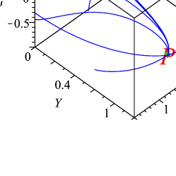
Refer to caption
(a)   m=0.5,n=0.6,γ=1formulae-sequence𝑚0.5formulae-sequence𝑛0.6𝛾1m=0.5,n=0.6,\gamma=1.
Refer to caption
(b)   m=0.75,n=0.05,γ=1formulae-sequence𝑚0.75formulae-sequence𝑛0.05𝛾1m=0.75,n=0.05,\gamma=1.
Refer to caption
(c)   m=0.9,n=0.4,γ=1formulae-sequence𝑚0.9formulae-sequence𝑛0.4𝛾1m=0.9,n=0.4,\gamma=1.
Refer to caption
(d)   m=2.0,n=0.5,γ=1formulae-sequence𝑚2.0formulae-sequence𝑛0.5𝛾1m=2.0,n=0.5,\gamma=1.
Refer to caption
(e)   m=0.3,n=0.5,γ=1formulae-sequence𝑚0.3formulae-sequence𝑛0.5𝛾1m=0.3,n=0.5,\gamma=1.
Figure 3: Some orbits in the phase plane of the system (57), (58), (59) for the five choices of the parameters and ε=+1𝜀1\varepsilon=+1.

The equilibrium points/lines of the system (57), (58), (59) (for a fixed sign of ε𝜀\varepsilon) have coordinates (Xϕ,Xψ,Y)subscript𝑋italic-ϕsubscript𝑋𝜓𝑌(X_{\phi},X_{\psi},Y):

  1. 1.

    O±:=(0,0,0)assignsubscript𝑂plus-or-minus000O_{\pm}:=(0,0,0).

    For ε=+1𝜀1\varepsilon=+1 we obtain a representation of the point O𝑂O referred in table 4.

  2. 2.

    C±:=(±1,Xψ,0)assignsubscript𝐶plus-or-minusplus-or-minus1superscriptsubscript𝑋𝜓0C_{\pm}:=(\pm 1,X_{\psi}^{\star},0) referred in table 4.

  3. 3.

    P±:=(mε2m2+3n2+3,nε2m2+3n2+3,P_{\pm}:=\Big{(}\frac{m\varepsilon}{\sqrt{-2m^{2}+3n^{2}+3}},-\frac{n\varepsilon}{\sqrt{-2m^{2}+3n^{2}+3}},
    3m2n212m23n23)\sqrt{3}\sqrt{\frac{m^{2}-n^{2}-1}{2m^{2}-3n^{2}-3}}\Big{)}. The point P𝑃P referred in table 4 is recovered by setting ε=+1𝜀1\varepsilon=+1.

  4. 4.

    T±:=(mε4(m2n2)2+2m2n2,nε4(m2n2)2+2m2n2,T_{\pm}:=\Big{(}\frac{m\varepsilon}{\sqrt{4\left(m^{2}-n^{2}\right)^{2}+2m^{2}-n^{2}}},-\frac{n\varepsilon}{\sqrt{4\left(m^{2}-n^{2}\right)^{2}+2m^{2}-n^{2}}},
    3m2n24(m2n2)2+2m2n2)\frac{\sqrt{3}\sqrt{m^{2}-n^{2}}}{\sqrt{4\left(m^{2}-n^{2}\right)^{2}+2m^{2}-n^{2}}}\Big{)}. The point T𝑇T referred in table 4 is recovered by setting ε=+1𝜀1\varepsilon=+1.

  5. 5.
    1. (a)

      S1:=(m3n22m2,n3n22m2,3m2n22m23n2)assignsubscript𝑆1𝑚3superscript𝑛22superscript𝑚2𝑛3superscript𝑛22superscript𝑚23superscript𝑚2superscript𝑛22superscript𝑚23superscript𝑛2S_{1}:=\left(-\frac{m}{\sqrt{3n^{2}-2m^{2}}},\frac{n}{\sqrt{3n^{2}-2m^{2}}},\sqrt{3}\sqrt{\frac{m^{2}-n^{2}}{2m^{2}-3n^{2}}}\right).

    2. (b)

      S2:=(m3n22m2,n3n22m2,3m2n22m23n2)assignsubscript𝑆2𝑚3superscript𝑛22superscript𝑚2𝑛3superscript𝑛22superscript𝑚23superscript𝑚2superscript𝑛22superscript𝑚23superscript𝑛2S_{2}:=\left(\frac{m}{\sqrt{3n^{2}-2m^{2}}},-\frac{n}{\sqrt{3n^{2}-2m^{2}}},\sqrt{3}\sqrt{\frac{m^{2}-n^{2}}{2m^{2}-3n^{2}}}\right). The static solutions S1subscript𝑆1S_{1} and S2subscript𝑆2S_{2} exists for n>0,nmnformulae-sequence𝑛0𝑛𝑚𝑛n>0,-n\leq m\leq n.

    3. (c)

      S3±:=(Xϕ,±1,0)assignsubscriptsubscript𝑆3plus-or-minussuperscriptsubscript𝑋italic-ϕplus-or-minus10{}_{\pm}S_{3}:=(X_{\phi}^{\star},\pm 1,0). The lines S3±subscriptsubscript𝑆3plus-or-minus{}_{\pm}S_{3} exists for 1Xϕ11superscriptsubscript𝑋italic-ϕ1-1\leq X_{\phi}^{\star}\leq 1.

    located at the curve S:=3Xψ2+2Y23=0assign𝑆3superscriptsubscript𝑋𝜓22superscript𝑌230S:=3X_{\psi}^{2}+2Y^{2}-3=0. They represent static universes H¯=H=0¯𝐻𝐻0\bar{H}=H=0.

In figure 3 (a), (b), (c), and (d) and (e) are presented some orbits in the phase plane of the system (57), (58), and (59) for ε=+1𝜀1\varepsilon=+1, that resembles the results found in 31 . The static universe configurations cannot by found in the framework of 31 . This illustrates the applicability of this formulation in compact variables.

III Alternative normalization

Due the negative sign of the kinetic energy of the phantom field, it is possible that H can be zero in a finite time. If so, the variables in 31 are not well defined as H0𝐻0H\rightarrow 0. They can diverge in a finite parameter time, whence the resulting system is not a dynamical system. To avoid this difficulty we will use an alternative set of dynamical variables, albeit non compact, similar to those introduced in Coley:2003mj section III.E, instead of the ones used in 31 , for investigating negative (and zero curvature models). For investigating positive curvature models we shall make use of similar variables to those defined in Coley:2003mj section VI.A.

III.1 Negative and zero curvature models

In this section we extent the analysis presented in Leon:2009ce , since now it is included the possibility of the crossing through H=0𝐻0H=0.

Let us introduce the following set of normalized variables: (D,Uϕ,Uψ,W,Ω)𝐷subscript𝑈italic-ϕsubscript𝑈𝜓𝑊Ω(D,\,U_{\phi},\,U_{\psi},\,W,\,\Omega), given by

D=3H1+9H2,Uϕ=32ϕ˙1+9H2,Uψ=32ψ˙1+9H2,formulae-sequence𝐷3𝐻19superscript𝐻2formulae-sequencesubscript𝑈italic-ϕ32˙italic-ϕ19superscript𝐻2subscript𝑈𝜓32˙𝜓19superscript𝐻2\displaystyle D=\frac{3H}{\sqrt{1+9H^{2}}},\;U_{\phi}=\sqrt{\frac{3}{2}}\frac{\dot{\phi}}{\sqrt{1+9H^{2}}},\;U_{\psi}=\sqrt{\frac{3}{2}}\frac{\dot{\psi}}{\sqrt{1+9H^{2}}},
W=3V1+9H2,Ω=3ρ1+9H2.formulae-sequence𝑊3𝑉19superscript𝐻2Ω3𝜌19superscript𝐻2\displaystyle W=\frac{\sqrt{3}V}{\sqrt{1+9H^{2}}},\,\Omega=\frac{3\rho}{1+9H^{2}}. (62)

This choice of phase-space variables renders the Friedmann equation as

D2(Uϕ2Uψ2+W2+Ω)=ΩkD20,superscript𝐷2superscriptsubscript𝑈italic-ϕ2superscriptsubscript𝑈𝜓2superscript𝑊2ΩsubscriptΩ𝑘superscript𝐷20\displaystyle D^{2}-\left(U_{\phi}^{2}-U_{\psi}^{2}+W^{2}+\Omega\right)=\Omega_{k}D^{2}\geq 0,
Ωk=ka2H2,k=1, 0.formulae-sequencesubscriptΩ𝑘𝑘superscript𝑎2superscript𝐻2𝑘1 0\displaystyle\Omega_{k}=-\frac{k}{a^{2}H^{2}},\;k=-1,\,0. (63)

By definition 1D1.1𝐷1-1\leq D\leq 1. Then,

0Uϕ2Uψ2+W2+ΩD21.0superscriptsubscript𝑈italic-ϕ2superscriptsubscript𝑈𝜓2superscript𝑊2Ωsuperscript𝐷210\leq U_{\phi}^{2}-U_{\psi}^{2}+W^{2}+\Omega\leq D^{2}\leq 1. (64)

From the requirement of the non-negativeness of the energy densities of quintom and matter, follows Ω=ΩmD20ΩsubscriptΩ𝑚superscript𝐷20\Omega=\Omega_{m}D^{2}\geq 0 and ΩdeD2Uϕ2Uψ2+W20subscriptΩ𝑑𝑒superscript𝐷2superscriptsubscript𝑈italic-ϕ2superscriptsubscript𝑈𝜓2superscript𝑊20\Omega_{de}D^{2}\equiv U_{\phi}^{2}-U_{\psi}^{2}+W^{2}\geq 0. Ωm,Ωde,ΩksubscriptΩ𝑚subscriptΩ𝑑𝑒subscriptΩ𝑘\Omega_{m},\,\Omega_{de},\,\Omega_{k} denotes the fractional energy densities of dark matter, dark energy and “curvature”. Then, from (64) follows that ΩΩ\Omega is bounded as ΩdesubscriptΩ𝑑𝑒\Omega_{de} is. However, we cannot guaranteed that the variables Uϕ,Uψ,subscript𝑈italic-ϕsubscript𝑈𝜓U_{\phi},\,U_{\psi}, W𝑊W are bounded. In this sense, the dynamical system constructed from the variables (62) is unbounded (then, non-compact). Hence, we cannot guaranteed that the system admits both future and past attractors. Numerical experience (see for instance 31 ) supports the conjecture that past and future attractors can exists depict unboundedness.

For D0𝐷0D\neq 0 (i.e., H0𝐻0H\neq 0) the variables (62) are related with those in 31 via

(xϕ2,xψ2,y2,z2)=(Uϕ2,Uψ2,W2,Ω)/D2.superscriptsubscript𝑥italic-ϕ2superscriptsubscript𝑥𝜓2superscript𝑦2superscript𝑧2superscriptsubscript𝑈italic-ϕ2superscriptsubscript𝑈𝜓2superscript𝑊2Ωsuperscript𝐷2\left(x_{\phi}^{2},\,x_{\psi}^{2},\,y^{2},\,z^{2}\right)=\left(U_{\phi}^{2},\,U_{\psi}^{2},\,W^{2},\,\Omega\right)/D^{2}. (65)

The equation of state (EoS) parameter, w,𝑤w, and the deceleration parameter, q,𝑞q, can be stated in terms of our variables as

w=Uϕ2Uψ2W2Uϕ2Uψ2+W2,q=1+Q/D2,formulae-sequence𝑤superscriptsubscript𝑈italic-ϕ2superscriptsubscript𝑈𝜓2superscript𝑊2superscriptsubscript𝑈italic-ϕ2superscriptsubscript𝑈𝜓2superscript𝑊2𝑞1𝑄superscript𝐷2w=\frac{U_{\phi}^{2}-U_{\psi}^{2}-W^{2}}{U_{\phi}^{2}-U_{\psi}^{2}+W^{2}},\,q=-1+Q/D^{2}, (66)

where

Q=D2+2(Uϕ2Uψ2)W2+12(3γ2)Ω.𝑄superscript𝐷22superscriptsubscript𝑈italic-ϕ2superscriptsubscript𝑈𝜓2superscript𝑊2123𝛾2ΩQ=D^{2}+2\left(U_{\phi}^{2}-U_{\psi}^{2}\right)-W^{2}+\frac{1}{2}\left(3\gamma-2\right)\Omega. (67)

The evolution equations for (62) are

D=13(1D2)Q,superscript𝐷131superscript𝐷2𝑄\displaystyle D^{\prime}=-\frac{1}{3}\left(1-D^{2}\right)Q,
Uϕ=D(1Q3)Uϕ+mW2,superscriptsubscript𝑈italic-ϕ𝐷1𝑄3subscript𝑈italic-ϕ𝑚superscript𝑊2\displaystyle U_{\phi}^{\prime}=-D\,\left(1-\frac{Q}{3}\right)\,U_{\phi}+m\,W^{2},
Uψ=D(1Q3)UψnW2,superscriptsubscript𝑈𝜓𝐷1𝑄3subscript𝑈𝜓𝑛superscript𝑊2\displaystyle U_{\psi}^{\prime}=-D\,\left(1-\frac{Q}{3}\right)\,U_{\psi}-n\,W^{2},
W=(13DQ+mUϕ+nUψ)W,superscript𝑊13𝐷𝑄𝑚subscript𝑈italic-ϕ𝑛subscript𝑈𝜓𝑊\displaystyle W^{\prime}=-\left(-\frac{1}{3}\,D\,Q+m\,U_{\phi}+n\,U_{\psi}\right)\,W,
Ω=D(23Q+γ)Ω,superscriptΩ𝐷23𝑄𝛾Ω\displaystyle\Omega^{\prime}=-D\,\left(-\frac{2}{3}\,Q+\gamma\right)\,\Omega, (68)

where we have defined the new independent variable

ddτ=11+9H2ddt.{}^{\prime}\equiv\frac{d}{d\tau}=\frac{1}{\sqrt{1+9H^{2}}}\frac{d}{dt}. (69)

The ODEs (68) define a flow on the state space

Ψ=Ψabsent\displaystyle\Psi= {(D,Uϕ,Uψ,W,Ω)5:\displaystyle\{\left(D,U_{\phi},U_{\psi},W,\Omega\right)\in\mathbb{R}^{5}: (70)
0Uϕ2Uψ2+W2+ΩD2,1D1,formulae-sequence0superscriptsubscript𝑈italic-ϕ2superscriptsubscript𝑈𝜓2superscript𝑊2Ωsuperscript𝐷21𝐷1\displaystyle 0\leq U_{\phi}^{2}-U_{\psi}^{2}+W^{2}+\Omega\leq D^{2},-1\leq D\leq 1,
Uϕ2Uψ2+W20,W0,Ω0}.\displaystyle U_{\phi}^{2}-U_{\psi}^{2}+W^{2}\geq 0,W\geq 0,\Omega\geq 0\}.

Observe that the variable D𝐷D does not decouples from the other variables. Hence, the system is of higher dimension (5-dimensional) that the system we can obtain by using the variables defined in 31 (4-dimensional in the case of negative curvature).

Remark 6.

In the case D=0𝐷0D=0 we find from (64) and from the requirement of non-negativeness of the energy densities of the sources, that Ω=0Ω0\Omega=0 and Uϕ2Uψ2+W2=0.superscriptsubscript𝑈italic-ϕ2superscriptsubscript𝑈𝜓2superscript𝑊20U_{\phi}^{2}-U_{\psi}^{2}+W^{2}=0. Then, Q|D=0=3W20D|D=0=13Q|D=0=W20.evaluated-at𝑄𝐷03superscript𝑊20evaluated-atsuperscript𝐷𝐷0evaluated-at13𝑄𝐷0superscript𝑊20Q|_{D=0}=-3W^{2}\leq 0\Rightarrow D^{\prime}|_{D=0}=-\frac{1}{3}Q|_{D=0}=W^{2}\geq 0. From the last inequality we can conclude that the submanifold D=0𝐷0D=0 is not invariant for models with W>0,𝑊0W>0, but acts as a membrane. For massless scalar field (MSF) cosmologies, the submanifold D=0𝐷0D=0 is invariant and is equivalent to the set Ω=0,Uϕ2Uψ2=0formulae-sequenceΩ0superscriptsubscript𝑈italic-ϕ2superscriptsubscript𝑈𝜓20\Omega=0,U_{\phi}^{2}-U_{\psi}^{2}=0.

The dynamical system (68) is invariant under the transformation of coordinates

(τ,D,Uϕ,Uψ,W,Ω)(τ,D,Uϕ,Uψ,W,Ω).𝜏𝐷subscript𝑈italic-ϕsubscript𝑈𝜓𝑊Ω𝜏𝐷subscript𝑈italic-ϕsubscript𝑈𝜓𝑊Ω\left(\tau,D,U_{\phi},U_{\psi},W,\Omega\right)\rightarrow\left(-\tau,-D,-U_{\phi},-U_{\psi},W,\Omega\right). (71)

Thus, it is sufficient to discuss the behavior in one part of the phase space. The dynamics in the other part being obtained via the transformation (71).

Remark 7.

Let be defined in the interior of the phase space the function

M=(nUϕ+mUψ)2Ω3(1D2)(D2Uϕ2+Uψ2W2Ω)3,𝑀superscript𝑛subscript𝑈italic-ϕ𝑚subscript𝑈𝜓2superscriptΩ31superscript𝐷2superscriptsuperscript𝐷2superscriptsubscript𝑈italic-ϕ2superscriptsubscript𝑈𝜓2superscript𝑊2Ω3\displaystyle M=\frac{{\left(n\,U_{\phi}+m\,U_{\psi}\right)}^{2}\,{\Omega}^{3}}{\left(1-D^{2}\right)\,{\left(D^{2}-{U_{\phi}}^{2}+{U_{\psi}}^{2}-W^{2}-\Omega\right)}^{3}},
M=3γDM.superscript𝑀3𝛾𝐷𝑀\displaystyle M^{\prime}=-3\gamma DM. (72)

This function is a monotonic function in the regions 0<D<10𝐷10<D<1 and 1<D<01𝐷0-1<D<0 for Ω>0Ω0\Omega>0 and nUϕ+mUψ0.𝑛subscript𝑈italic-ϕ𝑚subscript𝑈𝜓0n\,U_{\phi}+m\,U_{\psi}\neq 0. From the expression of M𝑀M we can see immediately that either D21superscript𝐷21D^{2}\rightarrow 1 or Ω0,Ω0\Omega\rightarrow 0, or nUϕ+mUψ0𝑛subscript𝑈italic-ϕ𝑚subscript𝑈𝜓0n\,U_{\phi}+m\,U_{\psi}\rightarrow 0 or |nUϕ+mUψ|+𝑛subscript𝑈italic-ϕ𝑚subscript𝑈𝜓\left|n\,U_{\phi}+m\,U_{\psi}\right|\rightarrow+\infty (which means that Uϕsubscript𝑈italic-ϕU_{\phi} or Uψsubscript𝑈𝜓U_{\psi} or both diverge) or Ωk0subscriptΩ𝑘0\Omega_{k}\rightarrow 0 asymptotically. Particularly, M𝑀M is a monotonic decreasing function for models with 0<D<10𝐷10<D<1 (i.e., for ever expanding models) and takes values in the interval (0,+).0(0,+\infty). Since M0𝑀0M\rightarrow 0 as Ω0Ω0\Omega\rightarrow 0 or as nUϕ+mUψ0𝑛subscript𝑈italic-ϕ𝑚subscript𝑈𝜓0n\,U_{\phi}+m\,U_{\psi}\rightarrow 0 (since its denominator is always bounded), then, the future asymptotic state of the system for ever expanding models corresponds to models with Ω=0Ω0\Omega=0 or to models where nUϕ+mUψ=0.𝑛subscript𝑈italic-ϕ𝑚subscript𝑈𝜓0n\,U_{\phi}+m\,U_{\psi}=0. Since M+𝑀M\rightarrow+\infty as |nUϕ+mUψ|+𝑛subscript𝑈italic-ϕ𝑚subscript𝑈𝜓\left|n\,U_{\phi}+m\,U_{\psi}\right|\rightarrow+\infty or as D1𝐷1D\rightarrow 1 or as Ωk0subscriptΩ𝑘0\Omega_{k}\rightarrow 0, then the past asymptotic state of the system for ever expanding models corresponds to models where at least one of the variables Uϕsubscript𝑈italic-ϕU_{\phi} or Uψsubscript𝑈𝜓U_{\psi} diverges, or to models with H𝐻H large, or to flat models.

The asymptotic dynamics for contracting models can determined from the asymptotic dynamics of ever expanding models by means of the coordinate transformation (71).

Remark 8.

The existence of the monotonic function (72) in our state space rules out any periodic, recurrent, or homoclinic orbit in the interior of the phase space. Therefore, some global results can be found from the linear (local) analysis of equilibrium points.

In the table 5 it is displayed the conditions for existence and the eigenvalues of the linearized system around each equilibrium point of the system (68). In table 6 we give the cosmological parameters associated to the equilibrium points. In the following we will characterize them.

Label (D,Uϕ,Uψ,W,Ω)𝐷subscript𝑈italic-ϕsubscript𝑈𝜓𝑊Ω(D,U_{\phi},U_{\psi},W,\Omega) Existence Eigenvalues
V1subscript𝑉1V_{1} (0,Uψ,Uψ,0,0)0superscriptsubscript𝑈𝜓superscriptsubscript𝑈𝜓00(0,-U_{\psi}^{\star},U_{\psi}^{\star},0,0) All m𝑚m and n𝑛n 0[×4],(mn)Uψ0[\times 4],(m-n)U_{\psi}^{\star}
V2subscript𝑉2V_{2} (0,Uψ,Uψ,0,0)0superscriptsubscript𝑈𝜓superscriptsubscript𝑈𝜓00(0,U_{\psi}^{\star},U_{\psi}^{\star},0,0) All m𝑚m and n𝑛n 0[×4],(m+n)Uψ0[\times 4],-(m+n)U_{\psi}^{\star}
K±±subscriptsubscript𝐾plus-or-minusplus-or-minus{}_{\pm}K_{\pm} (ϵ,±1+Uψ2,Uψ,0,0)italic-ϵplus-or-minus1superscriptsuperscriptsubscript𝑈𝜓2superscriptsubscript𝑈𝜓00(\epsilon,\pm\sqrt{1+{U_{\psi}^{\star}}^{2}},U_{\psi}^{\star},0,0) All m𝑚m and n𝑛n 2ϵ,43ϵ,0,ϵnUψmUϕ,ϵ(2γ)2italic-ϵ43italic-ϵ0italic-ϵ𝑛subscript𝑈𝜓𝑚subscript𝑈italic-ϕitalic-ϵ2𝛾2\epsilon,\frac{4}{3}\epsilon,0,\epsilon-nU_{\psi}-mU_{\phi},\epsilon(2-\gamma)
M±subscript𝑀plus-or-minus{}_{\pm}M (ϵ,0,0,0,0)italic-ϵ0000(\epsilon,0,0,0,0) All m𝑚m and n𝑛n 23,23,23ϵ,13ϵ,(γ23)ϵ232323italic-ϵ13italic-ϵ𝛾23italic-ϵ\frac{2}{3},-\frac{2}{3},-\frac{2}{3}\epsilon,\frac{1}{3}\epsilon,-\left(\gamma-\frac{2}{3}\right)\epsilon
F±subscript𝐹plus-or-minus{}_{\pm}F (ϵ,0,0,0,1)italic-ϵ0001(\epsilon,0,0,0,1) All m𝑚m and n𝑛n γϵ,γ2ϵ,(γ21)ϵ[×2],(γ23)ϵ\gamma\epsilon,\frac{\gamma}{2}\epsilon,\left(\frac{\gamma}{2}-1\right)\epsilon[\times 2],\left(\gamma-\frac{2}{3}\right)\epsilon
S±Fsubscript𝑆plus-or-minus𝐹{}_{\pm}SF (ϵ,mϵ,nϵ,1δ,0)italic-ϵ𝑚italic-ϵ𝑛italic-ϵ1𝛿0(\epsilon,m\epsilon,-n\epsilon,\sqrt{1-\delta},0) δ<1𝛿1\delta<1 2δϵ,2(13δ)ϵ,(1δ)ϵ[×2],(2δγ)ϵ2\delta\epsilon,-2\left(\frac{1}{3}-\delta\right)\epsilon,-\left(1-\delta\right)\epsilon[\times 2],\left(2\delta-\gamma\right)\epsilon
C±Ssubscript𝐶plus-or-minus𝑆{}_{\pm}CS (ϵ,mϵ3δ,nϵ3δ,23δ,0)italic-ϵ𝑚italic-ϵ3𝛿𝑛italic-ϵ3𝛿23𝛿0(\epsilon,\frac{m\epsilon}{3\delta},-\frac{n\epsilon}{3\delta},\frac{\sqrt{2}}{3\sqrt{\delta}},0) δ>13𝛿13\delta>\frac{1}{3} 23ϵ,23ϵ,(23γ)ϵ,13(1±43δ3)ϵ23italic-ϵ23italic-ϵ23𝛾italic-ϵ13plus-or-minus143𝛿3italic-ϵ\frac{2}{3}\epsilon,-\frac{2}{3}\epsilon,\left(\frac{2}{3}-\gamma\right)\epsilon,-\frac{1}{3}\left(1\pm\sqrt{\frac{4}{3\delta}-3}\right)\epsilon
M±Ssubscript𝑀plus-or-minus𝑆{}_{\pm}MS (ϵ,mγϵ2δ,nγϵ2δ,(2γ)γ2δ,1γ2δ)italic-ϵ𝑚𝛾italic-ϵ2𝛿𝑛𝛾italic-ϵ2𝛿2𝛾𝛾2𝛿1𝛾2𝛿(\epsilon,\frac{m\gamma\epsilon}{2\delta},-\frac{n\gamma\epsilon}{2\delta},\frac{\sqrt{(2-\gamma)\gamma}}{2\sqrt{\delta}},\sqrt{1-\frac{\gamma}{2\delta}}) δ>γ2𝛿𝛾2\delta>\frac{\gamma}{2} γϵ,(23γ)ϵ,(1+γ2)ϵ,λ±ϵ𝛾italic-ϵ23𝛾italic-ϵ1𝛾2italic-ϵsuperscript𝜆plus-or-minusitalic-ϵ\gamma\epsilon,-\left(\frac{2}{3}-\gamma\right)\epsilon,\left(-1+\frac{\gamma}{2}\right)\epsilon,\lambda^{\pm}\epsilon
Table 5: equilibrium points of quintom model with k=0,1𝑘01k=0,-1. We use the notations δ=m2n2𝛿superscript𝑚2superscript𝑛2\delta={m}^{2}-{n}^{2} and λ±=14(2γ±(2γ)(29γ+4γ2δ)).superscript𝜆plus-or-minus14plus-or-minus2𝛾2𝛾29𝛾4superscript𝛾2𝛿\displaystyle\lambda^{\pm}=-\frac{1}{4}\left(2-\gamma\pm\sqrt{(2-\gamma)\left(2-9\gamma+\frac{4\gamma^{2}}{\delta}\right)}\right). [×s][\times s] means multiplicity s. The subscripts on the label have the following significance. The left subscript gives the sign of D𝐷D (denoted by ϵ=±1italic-ϵplus-or-minus1\epsilon=\pm 1) and indicates whether the corresponding model is expanding (++) or contracting (-). The right subscript gives the sign of Uϕsubscript𝑈italic-ϕU_{\phi} (i.e., the sign of ϕ˙˙italic-ϕ\dot{\phi}) and is denoted by the sign ±plus-or-minus\pm. When the flow is restricted to the invariant sets D=±1,𝐷plus-or-minus1D=\pm 1, the eigenvalues associated to the equilibrium points M±,subscript𝑀plus-or-minus{}_{\pm}{M}, F±,subscript𝐹plus-or-minus{}_{\pm}{F}, S±Fsubscript𝑆plus-or-minus𝐹{}_{\pm}{SF} and M±Ssubscript𝑀plus-or-minus𝑆{}_{\pm}{MS} an to the equilibrium sets K^±±,subscriptsubscript^𝐾plus-or-minusplus-or-minus{}_{\pm}\hat{K}_{\pm}, are, in each case, the same as those displayed, but the first from the left.

The sets of equilibrium points V1,2subscript𝑉12V_{1,2} and K±±subscriptsubscript𝐾plus-or-minusplus-or-minus{}_{\pm}K_{\pm} and the isolated equilibrium points M±subscript𝑀plus-or-minus{}_{\pm}M are located in the invariant set of MSF cosmologies without matter. The isolated equilibrium point F±subscript𝐹plus-or-minus{}_{\pm}F is located in the invariant set of MSF cosmologies with matter.

V1,2subscript𝑉12V_{1,2} are degenerated equilibrium points. They represent flat vacuum static solutions (Ωde0,Ωm0,Ωk0).formulae-sequencesubscriptΩ𝑑𝑒0formulae-sequencesubscriptΩ𝑚0subscriptΩ𝑘0\left(\Omega_{de}\rightarrow 0,\Omega_{m}\rightarrow 0,\Omega_{k}\rightarrow 0\right).

The arcs K±±subscriptsubscript𝐾plus-or-minusplus-or-minus{}_{\pm}K_{\pm} denotes cosmological models dominated by dark energy (Ωde1subscriptΩ𝑑𝑒1\Omega_{de}\rightarrow 1) particularly by its kinetic energy. The DE mimics a stiff fluid solution. The stable (resp., unstable) manifold of K±subscriptsubscript𝐾plus-or-minus{}_{-}K_{\pm} (resp., K±+subscriptsubscript𝐾plus-or-minus{}_{+}K_{\pm} ) is at least 3-dimensional in the full phase space.

The equilibrium points M±subscript𝑀plus-or-minus{}_{\pm}M denotes the Milne’s universe. They are non hyperbolic for γ=23.𝛾23\gamma=\frac{2}{3}. The equilibrium points F±subscript𝐹plus-or-minus{}_{\pm}F represent the flat FRW universe. They are non-hyperbolic if γ=23𝛾23\gamma=\frac{2}{3} or γ=2.𝛾2\gamma=2. For γ>23,𝛾23\gamma>\frac{2}{3}, both M±subscript𝑀plus-or-minus{}_{\pm}M and P±subscript𝑃plus-or-minus{}_{\pm}P acts locally as saddles. The unstable (resp., stable) manifold of Msubscript𝑀{}_{-}M (resp. M+subscript𝑀{}_{+}M) is 3-dimensional in the full phase space. The equilibrium point M+subscript𝑀{}_{+}M (resp. Msubscript𝑀{}_{-}M) is unstable (resp. stable) to perturbations in D𝐷D and in W.𝑊W. The stable (resp., stable) manifold of Fsubscript𝐹{}_{-}F (resp. F+subscript𝐹{}_{+}F) is 3-dimensional. Whereas, the unstable (resp. stable) manifold Fsubscript𝐹{}_{-}F (resp. F+subscript𝐹{}_{+}F) is 2-dimensional in the full phase space. If we restrict the dynamics to the invariant sets with D2=1superscript𝐷21D^{2}=1 the dimensionality of all the above invariant sets reduces in one unity.

The isolated equilibrium points S±Fsubscript𝑆plus-or-minus𝐹{}_{\pm}SF and C±Ssubscript𝐶plus-or-minus𝑆{}_{\pm}CS denotes scalar field dominated solutions and curvature scaling solutions, respectively. They are located in the invariant set W>0,Ω=0.formulae-sequence𝑊0Ω0W>0,\Omega=0. The equilibrium points M±Ssubscript𝑀plus-or-minus𝑆{}_{\pm}MS (belonging to the invariant set W>0,Ω>0formulae-sequence𝑊0Ω0W>0,\Omega>0) represents flat matter scaling solutions. Observe that the equilibrium points M±Ssubscript𝑀plus-or-minus𝑆{}_{\pm}MS and S±Fsubscript𝑆plus-or-minus𝐹{}_{\pm}SF coincide as δγ2+𝛿superscript𝛾2\delta\rightarrow\frac{\gamma}{2}^{+} and C±Ssubscript𝐶plus-or-minus𝑆{}_{\pm}CS and S±Fsubscript𝑆plus-or-minus𝐹{}_{\pm}SF coincide as δ13+.𝛿superscript13\delta\rightarrow\frac{1}{3}^{+}. Additionally, S+Fsubscript𝑆𝐹{}_{+}SF (resp., SFsubscript𝑆𝐹{}_{-}SF) coincides with a point in the arc K++subscriptsubscript𝐾{}_{+}K_{+} (resp., Ksubscriptsubscript𝐾{}_{-}K_{-}) as δ1.𝛿superscript1\delta\rightarrow 1^{-}. These values of δ𝛿\delta where equilibrium points coincide corresponds to bifurcations.

Due the symmetry (71) it is sufficient to characterize the behavior of the equilibrium points S+F,subscript𝑆𝐹{}_{+}SF, C+S,subscript𝐶𝑆{}_{+}CS, and M+S.subscript𝑀𝑆{}_{+}MS. The dynamical character of their counterparts in the “negative” branch SF,subscript𝑆𝐹{}_{-}SF, CS,subscript𝐶𝑆{}_{-}CS, and MSsubscript𝑀𝑆{}_{-}MS is determined by the symmetry (71).

Label w𝑤w q𝑞q Ωm,Ωde,ΩksubscriptΩ𝑚subscriptΩ𝑑𝑒subscriptΩ𝑘\Omega_{m},\Omega_{de},\Omega_{k}
V1,2subscript𝑉12V_{1,2} indeterminate indeterminate indeterminate
K±±subscriptsubscript𝐾plus-or-minusplus-or-minus{}_{\pm}K_{\pm} 111 222 0,1,00100,1,0
M±subscript𝑀plus-or-minus{}_{\pm}M indeterminate 00 0,0,10010,0,1
F±subscript𝐹plus-or-minus{}_{\pm}F indeterminate 1+3γ213𝛾2-1+\frac{3\gamma}{2} 1,0,01001,0,0
S±Fsubscript𝑆plus-or-minus𝐹{}_{\pm}SF 1+2δ12𝛿-1+2\delta 1+3δ13𝛿-1+3\delta 0,1,00100,1,0
C±Ssubscript𝐶plus-or-minus𝑆{}_{\pm}CS 1313-\frac{1}{3} 00 0,13δ,113δ013𝛿113𝛿0,\frac{1}{3\delta},1-\frac{1}{3\delta}
M±Ssubscript𝑀plus-or-minus𝑆{}_{\pm}MS 1+γ1𝛾-1+\gamma 1+3γ213𝛾2-1+\frac{3\gamma}{2} 1γ2δ,γ2δ,01𝛾2𝛿𝛾2𝛿01-\frac{\gamma}{2\delta},\frac{\gamma}{2\delta},0
Table 6: Cosmological parameters associated to the equilibrium points.

The equilibrium point S+Fsubscript𝑆𝐹{}_{+}SF is non hyperbolic in the full phase space if either δ=13𝛿13\delta={\textstyle{1\over 3}} or δ=γ2𝛿𝛾2\delta={\textstyle{\gamma\over 2}} or δ=0.𝛿0\delta=0. However, if we restrict our attention to the flow in the invariant set D=1,𝐷1D=1, the eigenvalue 2δ2𝛿2\delta plays no role in the dynamics (it appears due the “extra” dimension, D𝐷D). In fact, if δ=0,𝛿0\delta=0, the eigenvalues of the system restricted to D=1𝐷1D=1 are (2/3,1[×2],γ(-2/3,-1[\times 2],-\gamma). Then, S+Fsubscript𝑆𝐹{}_{+}SF represents a de Sitter solution, and it is the attractor in the invariant set D=1.𝐷1D=1. If δ<0𝛿0\delta<0 and 23<γ<223𝛾2{\textstyle{2\over 3}}<\gamma<2 then, S+Fsubscript𝑆𝐹{}_{+}SF is the future attractor (in the full phase space) for (ever) expanding models and it represents a phantom field. Using the symmetry (71) we find that, if δ<0𝛿0\delta<0 and 23<γ<223𝛾2{\textstyle{2\over 3}}<\gamma<2 then, SFsubscript𝑆𝐹{}_{-}SF is the past attractor for contracting models and it represents a phantom field. If 0<δ<130𝛿130<\delta<{\textstyle{1\over 3}} and 23<γ<2,23𝛾2{\textstyle{2\over 3}}<\gamma<2, then S+Fsubscript𝑆𝐹{}_{+}SF represents a solution dominated by a quintessence field, and it is the future attractor for the flow restricted to the invariant set D=1𝐷1D=1. If 0<δ<130𝛿130<\delta<{\textstyle{1\over 3}} and 23<γ<2,23𝛾2{\textstyle{2\over 3}}<\gamma<2, then SFsubscript𝑆𝐹{}_{-}SF represents a solution dominated by a quintessence field, and it is the past attractor for the flow restricted to the invariant set D=1𝐷1D=-1.

The equilibrium point C+Ssubscript𝐶𝑆{}_{+}CS represents a solution with negative curvature. It is non hyperbolic if δ=13.𝛿13\delta={\textstyle{1\over 3}}. It is a saddle point for the full phase space, since it have always at least a positive eigenvalue. It is never a source (all the eigenvalues are not simultaneously with positive real parts) for the class of ever expanding models. By using the symmetry argument we find that CSsubscript𝐶𝑆{}_{-}CS is never a global attractor (or sink) for contracting models. But, if we restrict our attention to the flow in the invariant set D=1𝐷1D=1 we find that in this case C+Ssubscript𝐶𝑆{}_{+}CS is the future attractor provided δ>13𝛿13\delta>{\textstyle{1\over 3}} and 23<γ<2.23𝛾2{\textstyle{2\over 3}}<\gamma<2. In other words, one can say that if 23<γ<223𝛾2{\textstyle{2\over 3}}<\gamma<2 the spatial curvature destabilizes S+Fsubscript𝑆𝐹{}_{+}SF at the bifurcation value δ=13𝛿13\delta={\textstyle{1\over 3}} and that the stability is transferred to the equilibrium point C+Ssubscript𝐶𝑆{}_{+}CS (of course, this argument is valid only in the invariant set D=1𝐷1D=1).

The equilibrium point M+Ssubscript𝑀𝑆{}_{+}MS represents a cosmological solution where DE tracks DM (it means that the DE EoS parameter scales as the DM EoS parameter). It is non hyperbolic for γ=2/3𝛾23\gamma={2}/{3} or γ=2.𝛾2\gamma=2. It is in general a saddle point. However, when the dynamics is restricted to the invariant set D=1𝐷1D=1 it can be the future attractor (for ever expanding models) provided 0<γ<230𝛾230<\gamma<{\textstyle{2\over 3}} and δ>γ2.𝛿𝛾2\delta>{\textstyle{\gamma\over 2}}. From our hypothesis, this is not a region of physical interest. However, if we do not restrict the value of γ𝛾\gamma to be >23absent23>{\textstyle{2\over 3}} the above fact can be interpreted as follows. If 0<γ<230𝛾230<\gamma<{\textstyle{2\over 3}} the matter destabilizes S+Fsubscript𝑆𝐹{}_{+}SF at the bifurcation value δ=γ2𝛿𝛾2\delta={\textstyle{\gamma\over 2}} and that the stability is transferred to the equilibrium point M+S.subscript𝑀𝑆{}_{+}MS. Otherwise, whenever 0<γ<230𝛾230<\gamma<{\textstyle{2\over 3}} and δ<γ2𝛿𝛾2\delta<{\textstyle{\gamma\over 2}} the late time attractor in the invariant set D=1𝐷1D=1 is the equilibrium point S+F.subscript𝑆𝐹{}_{+}SF.

These equilibrium points are such that nUϕ+mUψ=0.𝑛subscript𝑈italic-ϕ𝑚subscript𝑈𝜓0n\,U_{\phi}+m\,U_{\psi}=0. Hence, by the structure of the function (72), for ever expanding models (i.e., for 0<D<10𝐷10<D<1), the late time behavior is determined by the local behavior of either S+Fsubscript𝑆𝐹{}_{+}SF or C+Ssubscript𝐶𝑆{}_{+}CS or M+S.subscript𝑀𝑆{}_{+}MS. By making use of the symmetry (71) it is possible to determine the early time behavior of contracting models (i.e, for 1<D<01𝐷0-1<D<0) from the local behavior of either SFsubscript𝑆𝐹{}_{-}SF or CSsubscript𝐶𝑆{}_{-}CS or MS.subscript𝑀𝑆{}_{-}MS. Combining the above linear analysis, with the information we have using monotonic functions we have the following

Proposition 7.

The past and future attractors of the quintom model with k=0,1𝑘01k=0,-1 are as follows:

  1. 1.

    For D=1𝐷1D=-1:

    1. (a)

      The past attractors are:

      1. i.

        SFsubscript𝑆𝐹{}_{-}SF if 23γ2, 0δ<13formulae-sequence23𝛾2 0𝛿13\frac{2}{3}\leq\gamma\leq 2,\,0\leq\delta<{\textstyle{1\over 3}} or
        0γ23, 0δ<γ2formulae-sequence0𝛾23 0𝛿𝛾20\leq\gamma\leq{\textstyle{2\over 3}},\,0\leq\delta<{\textstyle{\gamma\over 2}}.

      2. ii.

        CSsubscript𝐶𝑆{}_{-}CS if 23<γ<2,δ>13formulae-sequence23𝛾2𝛿13{\textstyle{2\over 3}}<\gamma<2,\,\delta>{\textstyle{1\over 3}}.

      3. iii.

        MSsubscript𝑀𝑆{}_{-}MS if 0<γ<23,δ>γ2formulae-sequence0𝛾23𝛿𝛾20<\gamma<{\textstyle{2\over 3}},\,\delta>{\textstyle{\gamma\over 2}}.

    2. (b)

      The future attractor is K±ifnUψ±m1+Uψ2>1plus-or-minussubscriptsubscript𝐾plus-or-minusif𝑛superscriptsubscript𝑈𝜓𝑚1superscriptsuperscriptsubscript𝑈𝜓21{}_{-}K_{\pm}\,\text{if}\;\,nU_{\psi}^{\star}\pm m\sqrt{1+{U_{\psi}^{\star}}^{2}}>-1.

  2. 2.

    For 1<D<01𝐷0-1<D<0

    1. (a)

      The past attractor is SFsubscript𝑆𝐹{}_{-}SF if 0γ2,δ<0formulae-sequence0𝛾2𝛿00\leq\gamma\leq 2,\,\delta<0.

    2. (b)

      The future attractor lies on K±ifnUψ±m1+Uψ2>1plus-or-minussubscriptsubscript𝐾plus-or-minusif𝑛superscriptsubscript𝑈𝜓𝑚1superscriptsuperscriptsubscript𝑈𝜓21{}_{-}K_{\pm}\,\text{if}\;\,nU_{\psi}^{\star}\pm m\sqrt{1+{U_{\psi}^{\star}}^{2}}>-1.

  3. 3.

    For 0<D<10𝐷10<D<1

    1. (a)

      The past attractor is K±+subscriptsubscript𝐾plus-or-minus{}_{+}K_{\pm} if nUψ±m1+Uψ2<1plus-or-minus𝑛superscriptsubscript𝑈𝜓𝑚1superscriptsuperscriptsubscript𝑈𝜓21nU_{\psi}^{\star}\pm m\sqrt{1+{U_{\psi}^{\star}}^{2}}<1.

    2. (b)

      The future attractor is S+Fsubscript𝑆𝐹{}_{+}SF if 0γ2,δ<0formulae-sequence0𝛾2𝛿00\leq\gamma\leq 2,\,\delta<0.

  4. 4.

    For D=1𝐷1D=1

    1. (a)

      The past attractor is K±+subscriptsubscript𝐾plus-or-minus{}_{+}K_{\pm} if nUψ±m1+Uψ2<1plus-or-minus𝑛superscriptsubscript𝑈𝜓𝑚1superscriptsuperscriptsubscript𝑈𝜓21nU_{\psi}^{\star}\pm m\sqrt{1+{U_{\psi}^{\star}}^{2}}<1.

    2. (b)

      The future attractors are

      1. i.

        S+Fsubscript𝑆𝐹{}_{+}SF if 23γ2, 0δ<13formulae-sequence23𝛾2 0𝛿13\frac{2}{3}\leq\gamma\leq 2,\,0\leq\delta<{\textstyle{1\over 3}} or 0γ23, 0δ<γ2formulae-sequence0𝛾23 0𝛿𝛾20\leq\gamma\leq{\textstyle{2\over 3}},\,0\leq\delta<{\textstyle{\gamma\over 2}}

      2. ii.

        C+Ssubscript𝐶𝑆{}_{+}CS if 23<γ<2,δ>13formulae-sequence23𝛾2𝛿13{\textstyle{2\over 3}}<\gamma<2,\,\delta>{\textstyle{1\over 3}}.

      3. iii.

        M+Ssubscript𝑀𝑆{}_{+}MS if 0<γ<23,δ>γ2formulae-sequence0𝛾23𝛿𝛾20<\gamma<{\textstyle{2\over 3}},\,\delta>{\textstyle{\gamma\over 2}}.

III.2 Positive curvature models (k=+1𝑘1k=+1)

In this section we reproduce the results found by one of us in Leon:2009ce . Introducing the normalization factor

D^=3H2+a2.^𝐷3superscript𝐻2superscript𝑎2\hat{D}=3\sqrt{H^{2}+a^{-2}}. (73)

we have

D^0H0,a+^𝐷0formulae-sequence𝐻0𝑎\hat{D}\rightarrow 0\Leftrightarrow H\rightarrow 0,\,a\rightarrow+\infty

(i.e., at a singularity). This means that it is not possible that D^^𝐷\hat{D} vanishes at a finite time. Now, using the normalized variables

Q0=3HD^,U^ϕ=32ϕ˙D^,U^ψ=32ψ˙D^,formulae-sequencesubscript𝑄03𝐻^𝐷formulae-sequencesubscript^𝑈italic-ϕ32˙italic-ϕ^𝐷subscript^𝑈𝜓32˙𝜓^𝐷\displaystyle Q_{0}=\frac{3H}{\hat{D}},\;\hat{U}_{\phi}=\sqrt{\frac{3}{2}}\frac{\dot{\phi}}{\hat{D}},\;\hat{U}_{\psi}=\sqrt{\frac{3}{2}}\frac{\dot{\psi}}{\hat{D}},
W^=3VD^,Ω=3ρD^.formulae-sequence^𝑊3𝑉^𝐷Ω3𝜌^𝐷\displaystyle\hat{W}=\frac{\sqrt{3}V}{\hat{D}},\,\Omega=\frac{3\rho}{\hat{D}}. (74)

From the Friedmann equation we find

0U^ϕ2U^ψ2+W^2=1Ω^10superscriptsubscript^𝑈italic-ϕ2superscriptsubscript^𝑈𝜓2superscript^𝑊21^Ω10\leq\hat{U}_{\phi}^{2}-\hat{U}_{\psi}^{2}+\hat{W}^{2}=1-\hat{\Omega}\leq 1 (75)

and by definition

1Q01.1subscript𝑄01-1\leq Q_{0}\leq 1. (76)

By the restrictions (75, 76), the state variables are in the state space

Ψ^=^Ψabsent\displaystyle\hat{\Psi}= {(Q0,U^ϕ,U^ψ,W^):0U^ϕ2U^ϕ2+W^21,\displaystyle\Big{\{}\left(Q_{0},\hat{U}_{\phi},\hat{U}_{\psi},\hat{W}\right):0\leq\hat{U}_{\phi}^{2}-\hat{U}_{\phi}^{2}+\hat{W}^{2}\leq 1,
1Q01}.\displaystyle-1\leq Q_{0}\leq 1\Big{\}}. (77)

As before, this state space is not compact.

Let us introduce the time coordinate

ddτ^=3D^ddt.{}^{\prime}\equiv\frac{d}{d\hat{\tau}}=\frac{3}{\hat{D}}\frac{d}{dt}.

D^^𝐷\hat{D} has the evolution equation

D^=3Q0D^(U^ϕ2U^ψ2+γ2Ω^)superscript^𝐷3subscript𝑄0^𝐷superscriptsubscript^𝑈italic-ϕ2superscriptsubscript^𝑈𝜓2𝛾2^Ω\hat{D}^{\prime}=-3Q_{0}\hat{D}\left(\hat{U}_{\phi}^{2}-\hat{U}_{\psi}^{2}+\frac{\gamma}{2}\hat{\Omega}\right)

where

Ω^=1(U^ϕ2U^ψ2+W^).^Ω1superscriptsubscript^𝑈italic-ϕ2superscriptsubscript^𝑈𝜓2^𝑊\hat{\Omega}=1-\left(\hat{U}_{\phi}^{2}-\hat{U}_{\psi}^{2}+\hat{W}\right).

This equation decouples from the other evolution equations. Thus, a reduced set of evolution equations is obtained.

Q0=(1Q02)(13(U^ϕ2U^ψ2+γ2Ω^)),superscriptsubscript𝑄01superscriptsubscript𝑄0213superscriptsubscript^𝑈italic-ϕ2superscriptsubscript^𝑈𝜓2𝛾2^Ω\displaystyle Q_{0}^{\prime}={\left(1-Q_{0}^{2}\right)\,\left(1-3\,\left({\hat{U}_{\phi}}^{2}-{\hat{U}_{\psi}}^{2}+\frac{\gamma}{2}\,\hat{\Omega}\right)\right)}, (78)
U^ϕ=3mW^2+3Q0U^ϕ(1+U^ϕ2U^ψ2+γ2Ω^),superscriptsubscript^𝑈italic-ϕ3𝑚superscript^𝑊23subscript𝑄0subscript^𝑈italic-ϕ1superscriptsubscript^𝑈italic-ϕ2superscriptsubscript^𝑈𝜓2𝛾2^Ω\displaystyle\hat{U}_{\phi}^{\prime}=3\,m\,\hat{W}^{2}+3\,Q_{0}\,\hat{U}_{\phi}\,\left(-1+{\hat{U}_{\phi}}^{2}-{\hat{U}_{\psi}}^{2}+\frac{\gamma}{2}\,\hat{\Omega}\right), (79)
U^ψ=3nW^2+3Q0U^ψ(1+U^ϕ2U^ψ2+γ2Ω^),superscriptsubscript^𝑈𝜓3𝑛superscript^𝑊23subscript𝑄0subscript^𝑈𝜓1superscriptsubscript^𝑈italic-ϕ2superscriptsubscript^𝑈𝜓2𝛾2^Ω\displaystyle\hat{U}_{\psi}^{\prime}=-3\,n\,\hat{W}^{2}+3\,Q_{0}\,\hat{U}_{\psi}\,\left(-1+{\hat{U}_{\phi}}^{2}-{\hat{U}_{\psi}}^{2}+\frac{\gamma}{2}\,\hat{\Omega}\right), (80)
W^=3W^(mU^ϕ+nU^ψQ0(U^ϕ2U^ψ2+γ2Ω^)).superscript^𝑊3^𝑊𝑚subscript^𝑈italic-ϕ𝑛subscript^𝑈𝜓subscript𝑄0superscriptsubscript^𝑈italic-ϕ2superscriptsubscript^𝑈𝜓2𝛾2^Ω\displaystyle\hat{W}^{\prime}=-3\,\hat{W}\left(m\,\hat{U}_{\phi}+n\,\hat{U}_{\psi}-Q_{0}\,\left({\hat{U}_{\phi}}^{2}-{\hat{U}_{\psi}}^{2}+\frac{\gamma}{2}\,\hat{\Omega}\right)\right). (81)

There is also an auxiliary evolution equation

Ω^=Q0(2(U^ϕ2U^ψ2)+γ(1Ω^))Ω^.superscript^Ωsubscript𝑄02superscriptsubscript^𝑈italic-ϕ2superscriptsubscript^𝑈𝜓2𝛾1^Ω^Ω\hat{\Omega}^{\prime}=-Q_{0}\,\left(-2\,\left({\hat{U}_{\phi}}^{2}-{\hat{U}_{\psi}}^{2}\right)+\gamma\,\left(1-\hat{\Omega}\right)\right)\,\hat{\Omega}. (82)

It is useful to express some cosmological parameters in terms of our state variables.

(Ωm,Ωde,Ωk)=(Ω^,1Ω^,Q021)/Q02.subscriptΩ𝑚subscriptΩ𝑑𝑒subscriptΩ𝑘^Ω1^Ωsuperscriptsubscript𝑄021superscriptsubscript𝑄02\left(\Omega_{m},\Omega_{de},\Omega_{k}\right)=\left(\hat{\Omega},1-\hat{\Omega},Q_{0}^{2}-1\right)/Q_{0}^{2}.

Observe that the system (81, 82) is invariant under the transformation of coordinates

(τ^,Q0,U^ϕ,U^ψ,W^,Ω^)(τ^,Q0,U^ϕ,U^ψ,W^,Ω^).^𝜏subscript𝑄0subscript^𝑈italic-ϕsubscript^𝑈𝜓^𝑊^Ω^𝜏subscript𝑄0subscript^𝑈italic-ϕsubscript^𝑈𝜓^𝑊^Ω\left(\hat{\tau},Q_{0},\hat{U}_{\phi},\hat{U}_{\psi},\hat{W},\hat{\Omega}\right)\rightarrow\left(-\hat{\tau},-Q_{0},-\hat{U}_{\phi},-\hat{U}_{\psi},\hat{W},\hat{\Omega}\right). (83)

Thus, it is sufficient to discuss the behavior in one part of the phase space. The dynamics in the other part being obtained via the transformation (83).

Remark 9.

The function

N=(nU^ϕ+mU^ψ)2Ω^2(1Q02)3,N=6γQ0Nformulae-sequence𝑁superscript𝑛subscript^𝑈italic-ϕ𝑚subscript^𝑈𝜓2superscript^Ω2superscript1superscriptsubscript𝑄023superscript𝑁6𝛾subscript𝑄0𝑁N=\frac{\left(n\,\hat{U}_{\phi}+m\,\hat{U}_{\psi}\right)^{2}\,\hat{\Omega}^{2}}{\left(1-Q_{0}^{2}\right)^{3}},\;N^{\prime}=-6\gamma\,Q_{0}\,N (84)

is monotonic in the regions Q0<0subscript𝑄00Q_{0}<0 and Q0>0subscript𝑄00Q_{0}>0 for Q021,nU^ϕ+nU^ψ0,Ω^>0.formulae-sequencesuperscriptsubscript𝑄021formulae-sequence𝑛subscript^𝑈italic-ϕ𝑛subscript^𝑈𝜓0^Ω0Q_{0}^{2}\neq 1,\,n\,\hat{U}_{\phi}+n\,\hat{U}_{\psi}\neq 0,\,\hat{\Omega}>0. Hence, there can be no periodic orbits or recurrent orbits in the interior of the phase space. Furthermore, it is possible to obtain global results. From the expression N𝑁N we can immediately see that asymptotically Q021superscriptsubscript𝑄021Q_{0}^{2}\rightarrow 1 or nU^ϕ+mU~ψ0𝑛subscript^𝑈italic-ϕ𝑚subscript~𝑈𝜓0n\hat{U}_{\phi}+m\tilde{U}_{\psi}\rightarrow 0 or Ω^0.^Ω0\hat{\Omega}\rightarrow 0.

In the table 7 it is summarize the location, existence conditions and the eigenvalues of the linearized system around each equilibrium point. In the following we will characterize the dynamical behavior of the cosmological solutions associated with them.

The equilibrium points K^±,F^±,SF^±subscript^𝐾plus-or-minussubscript^𝐹plus-or-minussubscript^𝑆𝐹plus-or-minus{}_{\pm}\hat{K},{}_{\pm}\hat{F},{}_{\pm}\hat{SF} and MS^±subscript^𝑀𝑆plus-or-minus{}_{\pm}\hat{MS} represents flat FRW solutions. They corresponds to the same cosmological solutions as the not hatted ones. We submit the reader to the early sections for the physical interpretation of them. Although CS^±subscript^𝐶𝑆plus-or-minus{}_{\pm}\hat{CS} represent a curvature scaling solution, it is different from C±Ssubscript𝐶plus-or-minus𝑆{}_{\pm}{CS} in the sense that it represents a positive curvature model.

By the above discussion, we will focus here on the dynamical character of the equilibrium points, not in its physical interpretation. As before, due the symmetry (83), we will characterize the equilibrium points corresponding to the “positive” branch. The dynamical behavior of the equilibrium points in the “negative” branch is determined by the transformation (83).

Observe that the equilibrium points MS^±subscript^𝑀𝑆plus-or-minus{}_{\pm}\hat{MS} and SF^±subscript^𝑆𝐹plus-or-minus{}_{\pm}\hat{SF} coincide as δγ2+𝛿superscript𝛾2\delta\rightarrow\frac{\gamma}{2}^{+} and CS^±subscript^𝐶𝑆plus-or-minus{}_{\pm}\hat{CS} and SF^±subscript^𝑆𝐹plus-or-minus{}_{\pm}\hat{SF} coincide as δ13.𝛿superscript13\delta\rightarrow\frac{1}{3}^{-}. Additionally, SF^+subscript^𝑆𝐹{}_{+}\hat{SF} (resp., SF^subscript^𝑆𝐹{}_{-}\hat{SF}) coincides with a point in the arc K^++subscriptsubscript^𝐾{}_{+}\hat{K}_{+} (resp., K^subscriptsubscript^𝐾{}_{-}\hat{K}_{-}) as δ1.𝛿superscript1\delta\rightarrow 1^{-}. These values of δ𝛿\delta where equilibrium points coincide corresponds to bifurcations. Combining the above linear analysis, with the information we have using monotonic functions we have the following

Proposition 8.

The past and future attractors for the quintom model with k=1𝑘1k=1 are as follows:

  1. 1.

    For Q0=1subscript𝑄01Q_{0}=-1

    1. (a)

      The past attractors are:

      1. i.

        SF^subscript^𝑆𝐹{}_{-}\hat{SF} if 0γ2,δ<γ2formulae-sequence0𝛾2𝛿𝛾20\leq\gamma\leq 2,\,\delta<{\textstyle{\gamma\over 2}}.

      2. ii.

        MS^subscript^𝑀𝑆{}_{-}\hat{MS} if 0<γ<2,δ>γ2formulae-sequence0𝛾2𝛿𝛾20<\gamma<2,\,\delta>{\textstyle{\gamma\over 2}}.

    2. (b)

      The future attractor is K^±subscriptsubscript^𝐾plus-or-minus{}_{-}\hat{K}_{\pm} if nUψ±m1+Uψ2>1plus-or-minus𝑛superscriptsubscript𝑈𝜓𝑚1superscriptsuperscriptsubscript𝑈𝜓21nU_{\psi}^{\star}\pm m\sqrt{1+{U_{\psi}^{\star}}^{2}}>-1.

  2. 2.

    For 1<Q0<01subscript𝑄00-1<Q_{0}<0

    1. (a)

      The past attractor are:

      1. i.

        SF^subscript^𝑆𝐹{}_{-}\hat{SF} if 23γ2,δ<13formulae-sequence23𝛾2𝛿13\frac{2}{3}\leq\gamma\leq 2,\,\delta<{\textstyle{1\over 3}} or 0γ23,δ<γ2formulae-sequence0𝛾23𝛿𝛾20\leq\gamma\leq{\textstyle{2\over 3}},\,\delta<{\textstyle{\gamma\over 2}}.

      2. ii.

        MS^subscript^𝑀𝑆{}_{-}\hat{MS} if 0<γ<23,δ>γ2formulae-sequence0𝛾23𝛿𝛾20<\gamma<{\textstyle{2\over 3}},\,\delta>{\textstyle{\gamma\over 2}}.

    2. (b)

      The future attractor is K^±subscriptsubscript^𝐾plus-or-minus{}_{-}\hat{K}_{\pm} if nUψ±m1+Uψ2>1plus-or-minus𝑛superscriptsubscript𝑈𝜓𝑚1superscriptsuperscriptsubscript𝑈𝜓21nU_{\psi}^{\star}\pm m\sqrt{1+{U_{\psi}^{\star}}^{2}}>-1.

  3. 3.

    For 0<Q0<10subscript𝑄010<Q_{0}<1

    1. (a)

      The past attractor is K^±+ifnUψ±m1+Uψ2<1plus-or-minussubscriptsubscript^𝐾plus-or-minusif𝑛superscriptsubscript𝑈𝜓𝑚1superscriptsuperscriptsubscript𝑈𝜓21{}_{+}\hat{K}_{\pm}\,\text{if}\;nU_{\psi}^{\star}\pm m\sqrt{1+{U_{\psi}^{\star}}^{2}}<1.

    2. (b)

      The future attractor is

      1. i.

        SF^+subscript^𝑆𝐹{}_{+}\hat{SF} if 23γ2,δ<13formulae-sequence23𝛾2𝛿13\frac{2}{3}\leq\gamma\leq 2,\,\delta<{\textstyle{1\over 3}}
        or 0γ23,δ<γ2formulae-sequence0𝛾23𝛿𝛾20\leq\gamma\leq{\textstyle{2\over 3}},\,\delta<{\textstyle{\gamma\over 2}}.

      2. ii.

        MS^+subscript^𝑀𝑆{}_{+}\hat{MS} if 0<γ<23,δ>γ2formulae-sequence0𝛾23𝛿𝛾20<\gamma<{\textstyle{2\over 3}},\,\delta>{\textstyle{\gamma\over 2}}.

  4. 4.

    For Q0=1subscript𝑄01Q_{0}=1

    1. (a)

      The past attractor is K^±+subscriptsubscript^𝐾plus-or-minus{}_{+}\hat{K}_{\pm} if nUψ±m1+Uψ2<1plus-or-minus𝑛superscriptsubscript𝑈𝜓𝑚1superscriptsuperscriptsubscript𝑈𝜓21nU_{\psi}^{\star}\pm m\sqrt{1+{U_{\psi}^{\star}}^{2}}<1.

    2. (b)

      The future attractors are:

      1. i.

        SF^+subscript^𝑆𝐹{}_{+}\hat{SF} if 0γ2,δ<γ2formulae-sequence0𝛾2𝛿𝛾20\leq\gamma\leq 2,\,\delta<{\textstyle{\gamma\over 2}}.

      2. ii.

        MS^+subscript^𝑀𝑆{}_{+}\hat{MS} if 0<γ<2,δ>γ2formulae-sequence0𝛾2𝛿𝛾20<\gamma<2,\,\delta>{\textstyle{\gamma\over 2}}.

Label (Q0,U^ϕ,U^ψ,W^)subscript𝑄0subscript^𝑈italic-ϕsubscript^𝑈𝜓^𝑊(Q_{0},\hat{U}_{\phi},\hat{U}_{\psi},\hat{W}) Existence Eigenvalues
S±subscript𝑆plus-or-minusS_{\pm} (0,U^ϕ,U^ψ,0),0subscript^𝑈italic-ϕsubscript^𝑈𝜓0(0,{\hat{U}_{\phi}},{\hat{U}_{\psi}},0), U^ϕ2U^ψ2=23γ3(2γ)superscriptsubscript^𝑈italic-ϕ2superscriptsubscript^𝑈𝜓223𝛾32𝛾{\hat{U}_{\phi}}^{2}-{\hat{U}_{\psi}}^{2}=\frac{2-3\gamma}{3(2-\gamma)} 0γ230𝛾230\leq\gamma\leq{\textstyle{2\over 3}} 0,±2(23γ),3nU~ψ3mU^ϕ0plus-or-minus223𝛾3𝑛subscript~𝑈𝜓3𝑚subscript^𝑈italic-ϕ0,\pm\sqrt{2(2-3\gamma)},-3n\tilde{U}_{\psi}-3m\hat{U}_{\phi}
K^±±subscriptsubscript^𝐾plus-or-minusplus-or-minus{}_{\pm}\hat{K}_{\pm} (ϵ,±1+Uψ2,Uψ,0)italic-ϵplus-or-minus1superscriptsuperscriptsubscript𝑈𝜓2superscriptsubscript𝑈𝜓0(\epsilon,\pm\sqrt{1+{U_{\psi}^{\star}}^{2}},U_{\psi}^{\star},0) All m𝑚m and n𝑛n 4ϵ,0,3(ϵnUψmUϕ),3(2γ)ϵ4italic-ϵ03italic-ϵ𝑛subscript𝑈𝜓𝑚subscript𝑈italic-ϕ32𝛾italic-ϵ4\epsilon,0,3\left(\epsilon-nU_{\psi}-mU_{\phi}\right),3(2-\gamma)\epsilon
F^±subscript^𝐹plus-or-minus{}_{\pm}\hat{F} (ϵ,0,0,0)italic-ϵ000(\epsilon,0,0,0) All m𝑚m and n𝑛n (3γ2)ϵ,32γϵ,3(γ21)ϵ[×2]\left(3\gamma-2\right)\epsilon,\frac{3}{2}\gamma\epsilon,3\left(\frac{\gamma}{2}-1\right)\epsilon[\times 2]
SF^±subscript^𝑆𝐹plus-or-minus{}_{\pm}\hat{SF} (ϵ,mϵ,nϵ,1δ)italic-ϵ𝑚italic-ϵ𝑛italic-ϵ1𝛿(\epsilon,m\epsilon,-n\epsilon,\sqrt{1-\delta}) δ<1𝛿1\delta<1 2(13δ)ϵ,3(1δ)ϵ[×2],3(2δγ)ϵ-2\left(1-3\delta\right)\epsilon,-3\left(1-\delta\right)\epsilon[\times 2],3\left(2\delta-\gamma\right)\epsilon
CS^±subscript^𝐶𝑆plus-or-minus{}_{\pm}\hat{CS} (3δϵ,mϵ3δ,nϵ3δ,23)3𝛿italic-ϵ𝑚italic-ϵ3𝛿𝑛italic-ϵ3𝛿23(\sqrt{3\delta}\epsilon,\frac{m\epsilon}{\sqrt{3\delta}},-\frac{n\epsilon}{\sqrt{3\delta}},\sqrt{\frac{2}{3}}) 0<δ<130𝛿130<\delta<\frac{1}{3} 3δϵ±49δ,23δϵ,(23γ)3δϵplus-or-minus3𝛿italic-ϵ49𝛿23𝛿italic-ϵ23𝛾3𝛿italic-ϵ-\sqrt{3\delta}\epsilon\pm\sqrt{4-9\delta},-2\sqrt{3\delta}\epsilon,(2-3\gamma)\sqrt{3\delta}\epsilon
MS^±subscript^𝑀𝑆plus-or-minus{}_{\pm}\hat{MS} (ϵ,mγ2δ,nγ2δ,(2γ)γ2δ,1γ2δ)italic-ϵ𝑚𝛾2𝛿𝑛𝛾2𝛿2𝛾𝛾2𝛿1𝛾2𝛿(\epsilon,\frac{m\gamma}{2\delta},-\frac{n\gamma}{2\delta},\frac{\sqrt{(2-\gamma)\gamma}}{2\sqrt{\delta}},\sqrt{1-\frac{\gamma}{2\delta}}) δ>γ2𝛿𝛾2\delta>\frac{\gamma}{2} (23γ)ϵ,3(1+γ2)ϵ,3λ±ϵ23𝛾italic-ϵ31𝛾2italic-ϵ3superscript𝜆plus-or-minusitalic-ϵ-\left(2-3\gamma\right)\epsilon,3\left(-1+\frac{\gamma}{2}\right)\epsilon,3\lambda^{\pm}\epsilon
Table 7: equilibrium points in the quintom model with k=+1.𝑘1k=+1. We use the same notation as in table 5. If γ=23,𝛾23\gamma=\frac{2}{3}, the set of equilibrium points, S,𝑆S, (corresponding to static solutions) reduces to two sets of equilibrium points analogous to V1,2subscript𝑉12V_{1,2} (see table 5). When the flow is restricted to the invariant sets Q0=±1,subscript𝑄0plus-or-minus1Q_{0}=\pm 1, the eigenvalues associated to the equilibrium points F^±,subscript^𝐹plus-or-minus{}_{\pm}\hat{F}, SF^±subscript^𝑆𝐹plus-or-minus{}_{\pm}\hat{SF} and MS^±subscript^𝑀𝑆plus-or-minus{}_{\pm}\hat{MS} an to the equilibrium sets K^±±,subscriptsubscript^𝐾plus-or-minusplus-or-minus{}_{\pm}\hat{K}_{\pm}, are, in each case, the same as those displayed, but the first from the left.

IV Integrability and algebraic solution

In this section we examine the integrability for the gravitational field equations of the quintom model by using two methods for the study of the integrability of dynamical systems. In particular we apply the symmetry analysis, we determine point transformations which leaves invariants the differential equations which provide also conservation laws. The second method that we assume is the singularity analysis where we are able to write the algebraic solution for the cosmological quintom model of our consideration.

IV.1 Symmetry analysis

The symmetry analysis has an important role for the study of the integrability and the determination of analytical solutions in gravitational theories Maharaj1 ; Maharaj2 ; Maharaj3 . There is a plethora of applications in the literature of the symmetry analysis in cosmological studies, in the dark energy models and in the modified theories of gravity, for instance see ns01 ; ns02 ; ns03 ; ns04 ; ns05 and references therein.

Consider now the point-like Lagrangian for the quintom cosmological model (1) with potential (2) in the spatially flat geometry and without any other matter source

L(a,a˙,ϕ,ϕ˙,ψ,ψ˙)=𝐿𝑎˙𝑎italic-ϕ˙italic-ϕ𝜓˙𝜓absent\displaystyle L\left(a,\dot{a},\phi,\dot{\phi},\psi,\dot{\psi}\right)=
3aa˙2+12a3(ϕ˙2ψ˙2)V0a3e6(mϕ+nψ).3𝑎superscript˙𝑎212superscript𝑎3superscript˙italic-ϕ2superscript˙𝜓2subscript𝑉0superscript𝑎3superscript𝑒6𝑚italic-ϕ𝑛𝜓\displaystyle-3a\dot{a}^{2}+\frac{1}{2}a^{3}\left(\dot{\phi}^{2}-\dot{\psi}^{2}\right)-V_{0}a^{3}e^{-\sqrt{6}(m\phi+n\psi)}. (85)

The field equations are the Euler-Lagrange equations of the later point-like Lagrangian plus the Hamiltonian constraint

3aa˙2+12a3(ϕ˙2ψ˙2)V0a3e6(mϕ+nψ)=0.3𝑎superscript˙𝑎212superscript𝑎3superscript˙italic-ϕ2superscript˙𝜓2subscript𝑉0superscript𝑎3superscript𝑒6𝑚italic-ϕ𝑛𝜓0\mathcal{H}\equiv-3a\dot{a}^{2}+\frac{1}{2}a^{3}\left(\dot{\phi}^{2}-\dot{\psi}^{2}\right)-V_{0}a^{3}e^{-\sqrt{6}(m\phi+n\psi)}=0. (86)

which is the first Friedmann equation.

By following the Noether symmetry analysis, for a recent review on the approach and more details for the method we refer the reader to ns04 , we find that the Lagrangian (85) admits the following two Noether symmetries, except the trivial autonomous symmetry,

X1=nϕmψ,X2=23aa+263(m+n)(ϕ+ψ),formulae-sequencesubscript𝑋1𝑛subscriptitalic-ϕ𝑚subscript𝜓subscript𝑋223𝑎subscript𝑎263𝑚𝑛subscriptitalic-ϕsubscript𝜓X_{1}=n\partial_{\phi}-m\partial_{\psi}~{},~{}X_{2}=\frac{2}{3}a\partial_{a}+\frac{2\sqrt{6}}{3\left(m+n\right)}\left(\partial_{\phi}+\partial_{\psi}\right), (87)

where the corresponding Noetherian conservation laws

Φ1=a3(nϕ˙+mψ˙),subscriptΦ1superscript𝑎3𝑛˙italic-ϕ𝑚˙𝜓\displaystyle\Phi_{1}=a^{3}\left(n\dot{\phi}+m\dot{\psi}\right), (88)
Φ2=4a2a˙+263(m+n)a3(ϕ˙ψ˙).subscriptΦ24superscript𝑎2˙𝑎263𝑚𝑛superscript𝑎3˙italic-ϕ˙𝜓\displaystyle\Phi_{2}=-4a^{2}\dot{a}+\frac{2\sqrt{6}}{3\left(m+n\right)}a^{3}\left(\dot{\phi}-\dot{\psi}\right). (89)

The three conservation laws, \mathcal{H}Φ1subscriptΦ1\ \Phi_{1} and Φ2subscriptΦ2\Phi_{2} are linear independent, and in-involution, that is {Φ1,Φ2}=0,{Φ1,}=0formulae-sequencesubscriptΦ1subscriptΦ20subscriptΦ10\left\{\Phi_{1},\Phi_{2}\right\}=0,~{}\left\{\Phi_{1},\mathcal{H}\right\}=0 and {Φ2,}=0subscriptΦ20\left\{\Phi_{2},\mathcal{H}\right\}=0, where {,}\left\{,\right\} denotes the Poisson bracket. Thus, we can refer that the gravitational field equations described by the Lagrangian (86) form a Liouville integrable dynamical system arnold .

Notice that the above conservation laws can be written in terms of the phase plane variables as

Φ16a˙a=nxϕ+mxψ,subscriptΦ16˙𝑎𝑎𝑛subscript𝑥italic-ϕ𝑚subscript𝑥𝜓\displaystyle\frac{\Phi_{1}}{\sqrt{6}\dot{a}a}=nx_{\phi}+mx_{\psi}, (90)
Φ24a˙a=xϕxψm+n1,subscriptΦ24˙𝑎𝑎subscript𝑥italic-ϕsubscript𝑥𝜓𝑚𝑛1\displaystyle\frac{\Phi_{2}}{4\dot{a}a}=\frac{x_{\phi}-x_{\psi}}{m+n}-1, (91)

such that at the invariant set {𝐱2:nxϕ+mxψ=0}conditional-set𝐱superscript2𝑛subscript𝑥italic-ϕ𝑚subscript𝑥𝜓0\{{\bf x}\in\mathbb{R}^{2}:nx_{\phi}+mx_{\psi}=0\} we have the trivial charge Φ1=0subscriptΦ10\Phi_{1}=0, whereas in the invariant set {𝐱2:xϕxψm+n=1}conditional-set𝐱superscript2subscript𝑥italic-ϕsubscript𝑥𝜓𝑚𝑛1\{{\bf x}\in\mathbb{R}^{2}:\frac{x_{\phi}-x_{\psi}}{m+n}=1\} we have the trivial charge Φ2=0subscriptΦ20\Phi_{2}=0.

Because of the nonlinearity of the differential equations it is not possible to write the analytical solution in closed-form by using well-known functions. Hence, we continue our analysis with the singularity analysis where the solution can be written by using Laurent expansions.

IV.2 Singularity analysis

Except from the symmetry analysis, singularity analysis is another approach to study the integrability of a given dynamical system. In singularity analysis integrability is not concerned with the display of explicit functions but with the demonstration of  a specific property, such that: the existence of a Laurent series for each of the dependent variables. The series may not be summable to an explicit form, but does represent an analytic function apart from any singular points. Moreover, the essential feature of this Laurent series is that it is an expansion about a particular type of movable critical point, a pole.

While the symmetry analysis is related with the existence of closed-form solutions or solutions expressed in terms of well-known first-order differential equations. There is a choice of the type of definitions for the symmetries which can be applied in the symmetry analysis, where different conclusions can be occurs. On the other hand, singularity analysis is straightforward in its application as it does not offer so many choices. Both methods are complementary leachrev .

The main steps for the application of the singularity analysis for a given differential equation are described by the ARS algorithm (from the initial of Ablowitz, Ramani and Segur) Abl1 ; Abl2 ; Abl3 . The latter algorithm has been used in various cosmological models to determine the integrability and write algebraic solutions, for instance see sig1 ; cots ; sig2 ; sig3 ; sig4 ; sig5 and references therein. For a demonstration on the application of the ARS algorithm we refer the reader in the review of Ramani et al. Ramani89 .

Consider the dynamical system (14), (15) and (16) which describes the evolution of the universe in a spatially flat FRW universe. We search for singular behaviour of the form

xϕ(t)subscript𝑥italic-ϕ𝑡\displaystyle x_{\phi}\left(t\right) =\displaystyle= xϕ0(tt0)p1,subscript𝑥italic-ϕ0superscript𝑡subscript𝑡0subscript𝑝1\displaystyle x_{\phi 0}\left(t-t_{0}\right)^{p_{1}}~{}\ ,~{} (92)
xψ(t)subscript𝑥𝜓𝑡\displaystyle x_{\psi}\left(t\right) =\displaystyle= xψ0(tt0)p2,subscript𝑥𝜓0superscript𝑡subscript𝑡0subscript𝑝2\displaystyle x_{\psi 0}\left(t-t_{0}\right)^{p_{2}}~{},~{} (93)
y(t)𝑦𝑡\displaystyle y\left(t\right) =\displaystyle= y0(tt0)p3subscript𝑦0superscript𝑡subscript𝑡0subscript𝑝3\displaystyle y_{0}\left(t-t_{0}\right)^{p_{3}} (94)

where t0subscript𝑡0t_{0} is an arbitrary constant and denotes the position of the singularity. Thus we find the unique leading-order behavior to be

xϕ(t)subscript𝑥italic-ϕ𝑡\displaystyle x_{\phi}\left(t\right) =\displaystyle= xϕ0(tt0)12,subscript𝑥italic-ϕ0superscript𝑡subscript𝑡012\displaystyle x_{\phi 0}\left(t-t_{0}\right)^{-\frac{1}{2}}\ ,~{} (95)
xψ(t)subscript𝑥𝜓𝑡\displaystyle x_{\psi}\left(t\right) =\displaystyle= xψ0(tt0)12,subscript𝑥𝜓0superscript𝑡subscript𝑡012\displaystyle x_{\psi 0}\left(t-t_{0}\right)^{-\frac{1}{2}}~{},~{} (96)
y(t)𝑦𝑡\displaystyle y\left(t\right) =\displaystyle= y0(tt0)12subscript𝑦0superscript𝑡subscript𝑡012\displaystyle y_{0}\left(t-t_{0}\right)^{-\frac{1}{2}} (97)

with constraint equation

1(xϕ0)2+(xψ0)2(y0)2=0.1superscriptsubscript𝑥italic-ϕ02superscriptsubscript𝑥subscript𝜓02superscriptsubscript𝑦0201-\left(x_{\phi 0}\right)^{2}+\left(x_{\psi_{0}}\right)^{2}-\left(y_{0}\right)^{2}=0. (98)

From the latter it follows that two of the coefficients of the leading-order terms are arbitrary constants. In particular are the two constants of integrations, recall that t0subscript𝑡0t_{0} is the third integration constant. Hence, we can conclude that equations (14), (15) and (16) form an integrable dynamical system. However, in order to verify it we proceed with the next steps of the ARS algorithm.

In order to determine the resonances, we substitute in the dynamical system 14), (15) and (16)  the following expressions

xϕ(t)subscript𝑥italic-ϕ𝑡\displaystyle x_{\phi}\left(t\right) =\displaystyle= xϕ0(tt0)12+ε1(tt0)12+ssubscript𝑥italic-ϕ0superscript𝑡subscript𝑡012subscript𝜀1superscript𝑡subscript𝑡012𝑠\displaystyle x_{\phi 0}\left(t-t_{0}\right)^{-\frac{1}{2}}+\varepsilon_{1}\left(t-t_{0}\right)^{-\frac{1}{2}+s}\ (99)
xψ(t)subscript𝑥𝜓𝑡\displaystyle~{}x_{\psi}\left(t\right) =\displaystyle= xψ0(tt0)12+ε2(tt0)12+ssubscript𝑥𝜓0superscript𝑡subscript𝑡012subscript𝜀2superscript𝑡subscript𝑡012𝑠\displaystyle x_{\psi 0}\left(t-t_{0}\right)^{-\frac{1}{2}}+\varepsilon_{2}\left(t-t_{0}\right)^{-\frac{1}{2}+s}~{} (100)
y(t)𝑦𝑡\displaystyle~{}y\left(t\right) =\displaystyle= y0(tt0)12+ε3(tt0)12+ssubscript𝑦0superscript𝑡subscript𝑡012subscript𝜀3superscript𝑡subscript𝑡012𝑠\displaystyle y_{0}\left(t-t_{0}\right)^{-\frac{1}{2}}+\varepsilon_{3}\left(t-t_{0}\right)^{-\frac{1}{2}+s} (101)

in which ε1,ε2,ε3subscript𝜀1subscript𝜀2subscript𝜀3\varepsilon_{1},~{}\varepsilon_{2},~{}\varepsilon_{3} are infinitesimal parameters. We follow the steps described in Ramani89 for the determination of the resonances in systems of differential equations we find the three resonances to be

s1=1,s2=0and s3=0.formulae-sequencesubscript𝑠11subscript𝑠20and subscript𝑠30s_{1}=-1~{},~{}s_{2}=0~{}\text{and }s_{3}=0.

Resonance s1=1subscript𝑠11s_{1}=-1 is important to exist in order the singularity analysis to succeed. In particular it is related with the movable singularity. On the other hand, the values zero of the other two resonances tell us that two of the coefficient terms for the leading-order behavior are integration constants of the problem. Moreover, because s2,s3=0subscript𝑠2subscript𝑠30s_{2},~{}s_{3}=0, the solution of the dynamical system is expressed by Right Painlevé series, that is,

xϕ(t)=xϕ0(tt0)12+xϕ1(tt0)+i=2xϕi(tt0)12+i2,subscript𝑥italic-ϕ𝑡subscript𝑥italic-ϕ0superscript𝑡subscript𝑡012subscript𝑥subscriptitalic-ϕ1𝑡subscript𝑡0subscript𝑖2subscript𝑥subscriptitalic-ϕ𝑖superscript𝑡subscript𝑡012𝑖2x_{\phi}\left(t\right)=x_{\phi 0}\left(t-t_{0}\right)^{-\frac{1}{2}}+x_{\phi_{1}}\left(t-t_{0}\right)+\sum\limits_{i=2}x_{\phi_{i}}\left(t-t_{0}\right)^{-\frac{1}{2}+\frac{i}{2}}, (102)
xψ(t)=xψ0(tt0)12+xψ1(tt0)+j=2xψj(tt0)12+j2,subscript𝑥𝜓𝑡subscript𝑥𝜓0superscript𝑡subscript𝑡012subscript𝑥subscript𝜓1𝑡subscript𝑡0subscript𝑗2subscript𝑥subscript𝜓𝑗superscript𝑡subscript𝑡012𝑗2x_{\psi}\left(t\right)=x_{\psi 0}\left(t-t_{0}\right)^{-\frac{1}{2}}+x_{\psi_{1}}\left(t-t_{0}\right)+\sum\limits_{j=2}x_{\psi_{j}}\left(t-t_{0}\right)^{-\frac{1}{2}+\frac{j}{2}}, (103)
y(t)=y0(tt0)12+y1(tt0)+k=2yk(tt0)12+k2,𝑦𝑡subscript𝑦0superscript𝑡subscript𝑡012subscript𝑦1𝑡subscript𝑡0subscript𝑘2subscript𝑦𝑘superscript𝑡subscript𝑡012𝑘2y\left(t\right)=y_{0}\left(t-t_{0}\right)^{-\frac{1}{2}}+y_{1}\left(t-t_{0}\right)+\sum\limits_{k=2}y_{k}\left(t-t_{0}\right)^{-\frac{1}{2}+\frac{k}{2}}, (104)

where the first coefficient constants xϕ1,xψ2subscript𝑥subscriptitalic-ϕ1subscript𝑥subscript𝜓2x_{\phi_{1}},~{}x_{\psi_{2}} and y1subscript𝑦1y_{1} are calculated to be

xϕ1subscript𝑥subscriptitalic-ϕ1\displaystyle x_{\phi_{1}} =\displaystyle= 23m(3+4(xϕ0)2)(y0),2\displaystyle\frac{2}{3}m\left(3+4\left(x_{\phi_{0}}\right)^{2}\right)\left(y_{0}\right)~{}^{2},~{} (105)
xψ1subscript𝑥subscript𝜓1\displaystyle x_{\psi_{1}} =\displaystyle= 23(3n4mxϕ0xψ0)(y0)2,233𝑛4𝑚subscript𝑥subscriptitalic-ϕ0subscript𝑥subscript𝜓0superscriptsubscript𝑦02\displaystyle-\frac{2}{3}\left(3n-4mx_{\phi_{0}}x_{\psi_{0}}\right)\left(y_{0}\right)^{2}~{},~{} (106)
y1=y03(mxϕ0((y0)21)3nxψ0).subscript𝑦1subscript𝑦03𝑚subscript𝑥subscriptitalic-ϕ0superscriptsubscript𝑦0213𝑛subscript𝑥subscript𝜓0y_{1}=\frac{y_{0}}{3}\left(mx_{\phi_{0}}\left(\left(y_{0}\right)^{2}-1\right)-3nx_{\psi_{0}}\right). (107)

Thus we can conclude that the dynamical system (14), (15) and (16) passes the singularity test and its algebraic solution is given by the Right Painlevé Series (102), (103), (103). From the latter we can infer that the leading-order term (95), i.e. the dominant behavior close to the singularity is an unstable solution.

We perform the same analysis for the complete dynamical system (8), (9), (10) and (11), where we find similar results. In particular the leading-order behavior is

xϕ(t)subscript𝑥italic-ϕ𝑡\displaystyle x_{\phi}\left(t\right) =\displaystyle= xϕ0(tt0)12,xψ(t)=xψ0(tt0)12,subscript𝑥italic-ϕ0superscript𝑡subscript𝑡012subscript𝑥𝜓𝑡subscript𝑥𝜓0superscript𝑡subscript𝑡012\displaystyle x_{\phi 0}\left(t-t_{0}\right)^{-\frac{1}{2}}\ ,~{}x_{\psi}\left(t\right)=x_{\psi 0}\left(t-t_{0}\right)^{-\frac{1}{2}}~{}, (108)
y(t)𝑦𝑡\displaystyle~{}y\left(t\right) =\displaystyle= y0(tt0)12,z(t)=z0(tt0)12subscript𝑦0superscript𝑡subscript𝑡012𝑧𝑡subscript𝑧0superscript𝑡subscript𝑡012\displaystyle y_{0}\left(t-t_{0}\right)^{-\frac{1}{2}}~{},~{}z\left(t\right)=z_{0}\left(t-t_{0}\right)^{-\frac{1}{2}} (109)

with constraint equation

1((xϕ0)2(xψ0)2)(y0)2+(z0)23(3γ2)=0.1superscriptsubscript𝑥italic-ϕ02superscriptsubscript𝑥subscript𝜓02superscriptsubscript𝑦02superscriptsubscript𝑧0233𝛾201-\left(\left(x_{\phi 0}\right)^{2}-\left(x_{\psi_{0}}\right)^{2}\right)-\left(y_{0}\right)^{2}+\frac{\left(z_{0}\right)^{2}}{3}\left(3\gamma-2\right)=0. (110)

and resonances s1=1subscript𝑠11s_{1}=-1, s2=0subscript𝑠20s_{2}=0, s3=0subscript𝑠30s_{3}=0 and s4=0subscript𝑠40s_{4}=0. Hence, we have the following proposition.

Proposition 9.

The dynamical system described the four first-order equations (8), (9), (10) and (11), passes the singularity test with leading-order terms given by (108). The algebraic solution is given by the Right Painlevé Series

𝐱(t)=𝐱0(tt0)12+𝐱1(tt0)+i=2𝐱i(tt0)12+i2,𝐱𝑡subscript𝐱0superscript𝑡subscript𝑡012subscript𝐱1𝑡subscript𝑡0subscript𝑖2subscript𝐱𝑖superscript𝑡subscript𝑡012𝑖2\mathbf{x}\left(t\right)=\mathbf{x}_{0}\left(t-t_{0}\right)^{-\frac{1}{2}}+\mathbf{x}_{1}\left(t-t_{0}\right)+\sum\limits_{i=2}\mathbf{x}_{i}\left(t-t_{0}\right)^{-\frac{1}{2}+\frac{i}{2}}, (111)

where 𝐱=(xϕ,xψ,y,z)𝐱subscript𝑥italic-ϕsubscript𝑥𝜓𝑦𝑧\mathbf{x=}\left(x_{\phi},x_{\psi},y,z\right) and constraint equation (110). From the form of the Laurent expansions we refer that the leading-order term describe a past attractor for the dynamical system.

V Concluding Remarks

We discussed some results concerning the asymptotic dynamics of quintom cosmologies with exponential potential. Using in a combined way several tools of the dynamical systems theory such as the linear stability analysis, Normal Forms calculations, Center manifold and Invariant Manifold Theorems, by developing Monotonic functions and implementing numerical solutions, one can find information bout the early time and late time behavior and at the intermediate stages of the evolution.

We have divided the analysis of the negative curvature and zero curvature models from the analysis of positive curvature models.

For negative or zero curvature models the physical behavior of a typical quintom cosmology as as follow. For ever expanding cosmologies, near the big-bang a typical model behaves like a flat FL model with stiff fluid (i.e. the dark energy mimics a stiff fluid) represented by the equilibrium set K++subscriptsubscript𝐾{}_{+}K_{+} or by K+subscriptsubscript𝐾{}_{+}K_{-} (parameterized by the real value Uψsuperscriptsubscript𝑈𝜓U_{\psi}^{\star}) depending if nUψ+m1+Uψ2𝑛superscriptsubscript𝑈𝜓𝑚1superscriptsuperscriptsubscript𝑈𝜓2nU_{\psi}^{\star}+m\sqrt{1+{U_{\psi}^{\star}}^{2}} or nUψm1+Uψ2𝑛superscriptsubscript𝑈𝜓𝑚1superscriptsuperscriptsubscript𝑈𝜓2nU_{\psi}^{\star}-m\sqrt{1+{U_{\psi}^{\star}}^{2}} is less than 1.11. If 23<γ<223𝛾2{\textstyle{2\over 3}}<\gamma<2 and δ<0𝛿0\delta<0 the late time dynamics is determined by S+Fsubscript𝑆𝐹{}_{+}SF, i.e. the model is accelerating, close to flatness (Ωk0subscriptΩ𝑘0\Omega_{k}\rightarrow 0) and dominated by phantom dark energy (Ωde1subscriptΩ𝑑𝑒1\Omega_{de}\rightarrow 1). This means, that typically, ever expanding quintom model crosses the phantom divide (it EoS parameter takes values less than 11-1). The intermediate dynamics is will be governed to a large extent by the fixed points C+S,subscript𝐶𝑆{}_{+}CS, M+S,subscript𝑀𝑆{}_{+}MS, and M+,subscript𝑀{}_{+}M, which have a lower dimensional stable manifold. For H𝐻H large and positive (i.e., in the invariant set D=1𝐷1D=1), the late time dynamics is determined by the equilibrium point S+Fsubscript𝑆𝐹{}_{+}SF provided δ<13𝛿13\delta<{\textstyle{1\over 3}} which represents quintessence (1<q<01𝑞0-1<q<0, i.e. 1<w<131𝑤13-1<w<-{\textstyle{1\over 3}} ) or a phantom field (q<1𝑞1q<-1, i.e. w<1𝑤1w<-1) if δ>0𝛿0\delta>0 or δ<0𝛿0\delta<0 respectively. If δ=0𝛿0\delta=0 it represents a de Sitter cosmological model. Curvature dominates the late time evolution in the invariant set D=1𝐷1D=1 whenever 23<γ<223𝛾2{\textstyle{2\over 3}}<\gamma<2 and δ>13.𝛿13\delta>{\textstyle{1\over 3}}.

On the other hand, for contracting models, the typical behavior is, in one sense, the reverse of the above, that is, if 23<γ<223𝛾2{\textstyle{2\over 3}}<\gamma<2 and δ<0𝛿0\delta<0 the early time dynamics is determined by SFsubscript𝑆𝐹{}_{-}SF, i.e. the model is accelerating, close to flatness (Ωk0subscriptΩ𝑘0\Omega_{k}\rightarrow 0) and dominated by phantom dark energy (Ωde1subscriptΩ𝑑𝑒1\Omega_{de}\rightarrow 1). The intermediate dynamics is will be governed to a large extent by the fixed points CS,subscript𝐶𝑆{}_{-}CS, MS,subscript𝑀𝑆{}_{-}MS, and F,subscript𝐹{}_{-}F, which have a lower dimensional stable manifold. For H𝐻H large and negative (i.e., in the invariant set D=1𝐷1D=-1), the early time dynamics is determined by the equilibrium point S+Fsubscript𝑆𝐹{}_{+}SF provided δ<13.𝛿13\delta<{\textstyle{1\over 3}}. Curvature dominates the early time evolution in the invariant set D=1𝐷1D=1 whenever 23<γ<223𝛾2{\textstyle{2\over 3}}<\gamma<2 and δ>13.𝛿13\delta>{\textstyle{1\over 3}}. A typical model behaves at late times like a flat FL model with stiff fluid (i.e. the dark energy mimics a stiff fluid) represented by the equilibrium set K+subscriptsubscript𝐾{}_{-}K_{+} or by Ksubscriptsubscript𝐾{}_{-}K_{-} (parameterized by the real value Uψsuperscriptsubscript𝑈𝜓U_{\psi}^{\star}) depending if nUψ+m1+Uψ2𝑛superscriptsubscript𝑈𝜓𝑚1superscriptsuperscriptsubscript𝑈𝜓2nU_{\psi}^{\star}+m\sqrt{1+{U_{\psi}^{\star}}^{2}} or nUψm1+Uψ2𝑛superscriptsubscript𝑈𝜓𝑚1superscriptsuperscriptsubscript𝑈𝜓2nU_{\psi}^{\star}-m\sqrt{1+{U_{\psi}^{\star}}^{2}} is greater than 1.1-1.

The physical interpretation of the equilibrium points corresponding to positive curvature models was given in Leon:2009ce . The physical behavior of a typical closed quintom cosmology is as follows Leon:2009ce . For ever expanding cosmologies, near the big-bang a typical model behaves like a flat FRW model with stiff fluid represented by the equilibrium set K^++subscriptsubscript^𝐾{}_{+}\hat{K}_{+} or by K^+subscriptsubscript^𝐾{}_{+}\hat{K}_{-}, depending on the choice of the values of the free parameters m,n𝑚𝑛m,n and xψsuperscriptsubscript𝑥𝜓x_{\psi}^{\star}. If δ<1/3𝛿13\delta<1/3 and 0<Q0<10subscript𝑄010<Q_{0}<1 the late time dynamics is determined by SF^+subscript^𝑆𝐹{}_{+}\hat{SF}, (with the same physical properties as S+Fsubscript𝑆𝐹{}_{+}{SF}). The intermediate dynamics will be governed to a large extent by the fixed points CS^+subscript^𝐶𝑆{}_{+}\hat{CS}, MS^+subscript^𝑀𝑆{}_{+}\hat{MS} and F^+subscript^𝐹{}_{+}\hat{F} which have the highest lower-dimensional stable manifold. For flat models (i.e., in the invariant set Q0=1subscript𝑄01Q_{0}=1), the late time dynamics is determined by the equilibrium point SF^+subscript^𝑆𝐹{}_{+}\hat{SF} provided δ<1/2𝛿12\delta<1/2 or MS^+subscript^𝑀𝑆{}_{+}\hat{MS} provided δ>1/2𝛿12\delta>1/2 .

For contracting models, the typical behavior is, in one sense, the reverse of the above. If δ<1/3𝛿13\delta<1/3 and 1<Q0<01subscript𝑄00-1<Q_{0}<0 the early time dynamics is determined by SF^subscript^𝑆𝐹{}_{-}\hat{SF}. The intermediate dynamics will be governed to a large extent by the fixed points CS^subscript^𝐶𝑆{}_{-}\hat{CS}, MS^subscript^𝑀𝑆{}_{-}\hat{MS}, F^subscript^𝐹{}_{-}\hat{F} which have the highest lower-dimensional stable manifold. For flat models (i.e., in the invariant set Q0=1subscript𝑄01Q_{0}=-1), the early time dynamics is determined by the equilibrium point SF^subscript^𝑆𝐹{}_{-}\hat{SF} (or MF^subscript^𝑀𝐹{}_{-}\hat{MF} ) provided δ<1/2𝛿12\delta<1/2 (δ>1/2𝛿12\delta>1/2). A typical model behaves at late times like a flat FRW model with stiff fluid (i.e. the dark energy mimics a stiff fluid) represented by the equilibrium set K^+subscriptsubscript^𝐾{}_{-}\hat{K}_{+} or by K^subscriptsubscript^𝐾{}_{-}\hat{K}_{-} depending on the choice of the values of the free parameters m,n𝑚𝑛m,n and xψsuperscriptsubscript𝑥𝜓x_{\psi}^{\star}.

Furthermore, we applied the symmetry analysis and the singularity analysis to determine the integrability of the quintom model. By using the Noether point symmetries in the case of the flat FRW geometry without any matter source we found that the point-like Lagrangian admits three linear-independent conservations laws which are in involution. Therefore, the field equations form a Liouville integrable dynamical system. However, because of the nonlinearity of the field equations that analytical solution can not be written in close-form expression.

On the other hand, by using the singularity analysis we were able to prove the integrability either when matter source exists and also the spatial curvature is not zero. We wrote the analytic solution of the field equations by using Painlevé Series by starting from a unstable singular solution.

The two methods, symmetries and singularities, are complementary, while in a future analysis will be of special interest to determine new analytical solutions for other kind of potentials.

Acknowledgments GL thanks to Department of Mathematics and to Vicerrectoría de Investigación y Desarrollo Tecnológico at Universidad Católica del Norte for financial support. AP acknowledges financial support of FONDECYT grant No. 3160121. JLM acknowledges to Consejo Nacional de Ciencia y Tecnología (CONACYT) of Mexico for financial support throughout the Phd program on Water Sciences and Technology, Grant No. 003497.

Appendix A Invariant sets and monotonic functions

In the following we shall investigate some invariant sets that can be trivially identified and we construct properly monotonic functions defined on them.

Recall the definition and results:

Definition 1 (Invariant set).

Let Sn𝑆superscript𝑛S\subset\mathbb{R}^{n} be a set. S𝑆S is called an invariant set under the vector field

𝐱=𝐗(𝐱)superscript𝐱𝐗𝐱\mathbf{x}^{\prime}={\bf X}(\mathbf{x}) (112)

if 𝐲S𝐲𝑆\mathbf{y}\in S implies 𝐱(τ,𝐲)S𝐱𝜏𝐲𝑆\mathbf{x}(\tau,\mathbf{y})\in S (where 𝐱(0,𝐲)=𝐲𝐱0𝐲𝐲\mathbf{x}(0,\mathbf{y})=\mathbf{y}) for all τ.𝜏\tau\in\mathbb{R}. If we consider the property valid for τ0𝜏0\tau\geq 0 we say that S𝑆S is positively invariant. On the other hand, if the property is valid for τ0𝜏0\tau\leq 0 we say that S𝑆S is negatively invariant.

Proposition 10 (Proposition 4.1, reza p. 92).

Consider the autonomous vector field (112) with flow 𝐠τ.superscript𝐠𝜏\mathbf{g}^{\tau}. Let be defined a C1superscript𝐶1C^{1} function Z:n:𝑍superscript𝑛Z:\mathbb{R}^{n}\rightarrow\mathbb{R} which satisfies ZZ𝐗(𝐱)=αZsuperscript𝑍𝑍𝐗𝐱𝛼𝑍Z^{\prime}\equiv\nabla Z\cdot{\bf X}(\mathbf{x})=\alpha Z where α:n:𝛼superscript𝑛\alpha:\mathbb{R}^{n}\rightarrow\mathbb{R} is a continuous function. Then, the subsets of nsuperscript𝑛\mathbb{R}^{n} defined by {𝐱n|Z(𝐱)0}conditional-set𝐱superscript𝑛less-than-or-equals-or-greater-than𝑍𝐱0\left\{\mathbf{x}\in\mathbb{R}^{n}|Z(\mathbf{x})\lesseqqgtr 0\right\} are invariant sets for the flow 𝐠τ.superscript𝐠𝜏\mathbf{g}^{\tau}.

Definition 2 (Definition 4.8 reza , p. 93).

Let 𝐠τ(𝐱)superscript𝐠𝜏𝐱\mathbf{g}^{\tau}(\mathbf{x}) be a flow on n,superscript𝑛\mathbb{R}^{n}, let S𝑆S be an invariant set of 𝐠τ(𝐱)superscript𝐠𝜏𝐱\mathbf{g}^{\tau}(\mathbf{x}) and let Z:S:𝑍𝑆Z:S\rightarrow\mathbb{R} be a continuous function. Z𝑍Z is monotonic decreasing (increasing) function for the flow 𝐠τ(𝐱)superscript𝐠𝜏𝐱\mathbf{g}^{\tau}(\mathbf{x}) means that for all 𝐱S,𝐱𝑆\mathbf{x}\in S, Z(𝐠τ(𝐱))𝑍superscript𝐠𝜏𝐱Z(\mathbf{g}^{\tau}(\mathbf{x})) is a monotonic decreasing (increasing) function of τ.𝜏\tau.

The existence of a continuous monotone function on an invariant set S𝑆S simplifies the orbits in S𝑆S significantly. As states the following proposition.

Proposition 11 (Proposition 4.2 (reza , pp 93)).

The existence of a continuous monotone function on an invariant set S𝑆S implies that S𝑆S contains no equilibrium points, periodic orbits, recurrent orbits or homoclinic orbits.

Theorem 1 (Monotonicity Principle (Proposition A.I in LeBlanc:1994qm developed in collaboration with M Glaum, cited as Theorem 4.12 in reza )).

Let 𝐠τ(𝐱)superscript𝐠𝜏𝐱\mathbf{g}^{\tau}(\mathbf{x}) be a flow on nsuperscript𝑛\mathbb{R}^{n} with S𝑆S an invariant set. Let Z:S:𝑍𝑆Z:S\rightarrow\mathbb{R} be a C1(n)superscript𝐶1superscript𝑛C^{1}\left(\mathbb{R}^{n}\right) function whose range is the interval (a,b)𝑎𝑏(a,\;b) where a{},𝑎a\in\mathbb{R}\cup\{-\infty\}, b{+},𝑏b\in\mathbb{R}\cup\{+\infty\}, and a<b.𝑎𝑏a<b. If Z𝑍Z is decreasing on orbits in S,𝑆S, then for all 𝐱S𝐱𝑆\mathbf{x}\in S, ω(𝐱){𝐬S¯S|lim𝐲𝐬Z(𝐲)b}𝜔𝐱conditional-set𝐬¯𝑆𝑆𝑙𝑖subscript𝑚𝐲𝐬𝑍𝐲𝑏\omega(\mathbf{x})\subset\{\mathbf{s}\in\bar{S}\setminus S|lim_{\mathbf{y}\rightarrow\mathbf{s}}Z(\mathbf{y})\neq b\} and α(𝐱){𝐬S¯S|lim𝐲𝐬Z(𝐲)a}.𝛼𝐱conditional-set𝐬¯𝑆𝑆𝑙𝑖subscript𝑚𝐲𝐬𝑍𝐲𝑎\alpha(\mathbf{x})\subset\{\mathbf{s}\in\bar{S}\setminus S|lim_{\mathbf{y}\rightarrow\mathbf{s}}Z(\mathbf{y})\neq a\}.

Appendix B Normal Forms for vector fields

Let 𝐗:nn:𝐗superscript𝑛superscript𝑛{\bf X}:\mathbb{R}^{n}\rightarrow\mathbb{R}^{n} be a smooth vector field satisfying 𝐗(𝟎)=𝟎.𝐗00{\bf X}({\bf 0})={\bf 0}. We can formally construct the Taylor expansion of 𝐱𝐱{\bf x} about 𝟎,0{\bf 0}, namely, 𝐗=𝐗1+𝐗2++𝐗k+O(|𝐱|k+1),𝐗subscript𝐗1subscript𝐗2subscript𝐗𝑘𝑂superscript𝐱𝑘1{\bf X}={\bf X}_{1}+{\bf X}_{2}+\ldots+{\bf X}_{k}+{O}(|{\bf x}|^{k+1}), where 𝐗rHr,subscript𝐗𝑟superscript𝐻𝑟{\bf X}_{r}\in H^{r}, the real vector space of vector fields whose components are homogeneous polynomials of degree r𝑟r. For r=1𝑟1r=1 to k𝑘k we write

𝐗r(𝐱)=m1=1rmn=1rj=1n𝐗𝐦,j𝐱𝐦𝐞j,subscript𝐗𝑟𝐱superscriptsubscriptsubscript𝑚11𝑟superscriptsubscriptsubscript𝑚𝑛1𝑟superscriptsubscript𝑗1𝑛subscript𝐗𝐦𝑗superscript𝐱𝐦subscript𝐞𝑗\displaystyle{\bf X}_{r}({\bf x})=\sum_{m_{1}=1}^{r}\ldots\sum_{m_{n}=1}^{r}\sum_{j=1}^{n}{\bf X}_{{\bf m},j}{{\bf x}}^{{\bf m}}{\bf e}_{j},
imi=r,subscript𝑖subscript𝑚𝑖𝑟\displaystyle\sum_{i}m_{i}=r, (113)

Observe that 𝐗1=𝐃𝐗(𝟎)𝐱𝐀𝐱,subscript𝐗1𝐃𝐗0𝐱𝐀𝐱{\bf X}_{1}={\bf DX(\mathbf{0})}{\bf x}\equiv{\bf A}{\bf x}, i.e., the matrix of derivatives.

We have the following result

Theorem 2 (theorem 2.3.1 in arrowsmith ).

Given a smooth vector field 𝐗(𝐱)𝐗𝐱\bf X({\bf x}) on nsuperscript𝑛\mathbb{R}^{n} with 𝐗(𝟎)=𝟎,𝐗00{\bf X(0)=0}, there is a polynomial transformation to new coordinates, 𝐲,𝐲{\bf y}, such that the differential equation 𝐱=𝐗(𝐱)superscript𝐱𝐗𝐱{\bf x}^{\prime}={\bf X}({\bf x}) takes the form 𝐲=𝐉𝐲+r=1N𝐰r(𝐲)+O(|𝐲|N+1),superscript𝐲𝐉𝐲superscriptsubscript𝑟1𝑁subscript𝐰𝑟𝐲𝑂superscript𝐲𝑁1{\bf y}^{\prime}={\bf J}{\bf y}+\sum_{r=1}^{N}{\bf w}_{r}({\bf y})+{O}(|{\bf y}|^{N+1}), where 𝐉𝐉{\bf J} is the real Jordan form of 𝐀=𝐃𝐗(𝟎)𝐀𝐃𝐗0{\bf A}={\bf DX}({\bf 0}) and 𝐰rGr,subscript𝐰𝑟superscript𝐺𝑟{\bf w}_{r}\in G^{r}, a complementary subspace of Hrsuperscript𝐻𝑟H^{r} on Br=𝐋𝐀(Hr),superscript𝐵𝑟subscript𝐋𝐀superscript𝐻𝑟B^{r}={\bf L_{A}}(H^{r}), where 𝐋𝐀subscript𝐋𝐀{\bf L_{A}} is the linear operator that assigns to 𝐡(𝐲)Hr𝐡𝐲superscript𝐻𝑟{\bf h(y)}\in H^{r} the Lie bracket of the vector fields 𝐀𝐲𝐀𝐲{\bf Ay} and 𝐡(𝐲)𝐡𝐲{\bf h(y)}:

𝐋𝐀:Hr:subscript𝐋𝐀superscript𝐻𝑟\displaystyle{\bf L_{A}}:H^{r} Hrabsentsuperscript𝐻𝑟\displaystyle\rightarrow H^{r}
𝐡𝐡\displaystyle{\bf h} 𝐋𝐀𝐡(𝐲)=𝐃𝐡(𝐲)𝐀𝐲𝐀𝐡(𝐲).absentsubscript𝐋𝐀𝐡𝐲𝐃𝐡𝐲𝐀𝐲𝐀𝐡𝐲\displaystyle\rightarrow{\bf L_{A}}{\bf h(y)}={\bf Dh(y)}{\bf Ay}-{\bf Ah(y)}. (114)

References

  • (1) A. G. Riess et al. [Supernova Search Team], Astron. J.  116, 1009 (1998) [astro-ph/9805201].
  • (2) B. P. Schmidt et al. [Supernova Search Team], Astrophys. J.  507, 46 (1998) [astro-ph/9805200].
  • (3) W. L. Freedman et al. [HST Collaboration], Astrophys. J.  553, 47 (2001) [astro-ph/0012376].
  • (4) J. R. Mould et al., Astrophys. J.  529, 786 (2000) [astro-ph/9909260].
  • (5) P. Astier, J. Phys. Conf. Ser. 110, 012005 (2008)
  • (6) P. Astier et al. [SNLS Collaboration], Astron. Astrophys.  447, 31 (2006) [astro-ph/0510447].
  • (7) A. G. Riess et al. [Supernova Search Team], Astrophys. J.  607, 665 (2004) [astro-ph/0402512].
  • (8) J. Dunkley et al. [WMAP Collaboration], Astrophys. J. Suppl.  180, 306 (2009) [arXiv:0803.0586 [astro-ph]].
  • (9) D. N. Spergel et al. [WMAP Collaboration], Astrophys. J. Suppl.  170, 377 (2007) [astro-ph/0603449].
  • (10) D. N. Spergel et al. [WMAP Collaboration], Astrophys. J. Suppl.  148, 175 (2003) [astro-ph/0302209].
  • (11) A. C. S. Readhead et al., Astrophys. J.  609, 498 (2004) [astro-ph/0402359].
  • (12) J. H. Goldstein et al., Astrophys. J.  599, 773 (2003) [astro-ph/0212517].
  • (13) . J. K. Adelman-McCarthy et al. [SDSS Collaboration], Astrophys. J. Suppl.  175, 297 (2008) [arXiv:0707.3413 [astro-ph]].
  • (14) J. K. Adelman-McCarthy et al. [SDSS Collaboration], Astrophys. J. Suppl.  162, 38 (2006) [astro-ph/0507711].
  • (15) M. Tegmark et al. [SDSS Collaboration], Phys. Rev. D 74, 123507 (2006) [astro-ph/0608632].
  • (16) M. Tegmark et al. [SDSS Collaboration], Phys. Rev. D 69, 103501 (2004) [astro-ph/0310723].
  • (17) V. Sahni and A. Starobinsky, Int. J. Mod. Phys. D 15, 2105 (2006) [astro-ph/0610026].
  • (18) E. J. Copeland, M. Sami and S. Tsujikawa, Int. J. Mod. Phys. D 15, 1753 (2006) [hep-th/0603057].
  • (19) B. Feng, X. L. Wang and X. M. Zhang, Phys. Lett. B 607, 35 (2005) doi:10.1016/j.physletb.2004.12.071 [astro-ph/0404224].
  • (20) H. Wei and R. G. Cai, Phys. Lett. B 634, 9 (2006) [astro-ph/0512018].
  • (21) H. M. Sadjadi, M. Alimohammadi, Phys. Rev. D 74, 043506 (2006). arXiv:gr-qc/0605143.
  • (22) Z. K. Guo, Phys. Lett. B 608, 177 (2005).
  • (23) M. -Z. Li, B. Feng, X.-M. Zhang, JCAP 0512, 002 (2005).
  • (24) B. Feng, M. Li, Y.-S. Piao, X. Zhang, Phys. Lett. B 634, 101 (2006).
  • (25) M. R. Setare, Phys. Lett. B 641, 130 (2006).
  • (26) W. Zhao, Y. Zhang, Phys. Rev. D 73, 123509 (2006).
  • (27) M. R. Setare, E.N. Saridakis, Phys. Lett. B 671, 331 (2009). arXiv:0810.0645 [hep-th].
  • (28) H. Wei, R.G. Cai, Phys. Rev. D 72, 123507 (2005). arXiv:astro-ph/0509328.
  • (29) H. Wei, R.G. Cai, D.F. Zeng, Class. Quant. Gravit. 22, 3189 (2005). arXiv:hep-th/0501160.
  • (30) Z.K. Guo, Y.S. Piao, X.M. Zhang, Y.Z. Zhang, Phys. Lett. B 608, 177 (2005). arXiv:astro-ph/0410654.
  • (31) R. Lazkoz, G. Leon, Phys. Lett. B 638, 303 (2006). arXiv:astro-ph/0602590.
  • (32) X. F. Zhang, H. Li, Y.S. Piao, X.M. Zhang, Mod. Phys. Lett. A 21, 231 (2006). arXiv:astro-ph/0501652.
  • (33) Y. F. Cai, M. Z. Li, J. X. Lu, Y. S. Piao, T. T. Qiu, X. M. Zhang, Phys. Lett. B 651, 1 (2007). arXiv:hep-th/0701016.
  • (34) S. Zhang, B. Chen, arXiv:0806.4435 [hep-ph].
  • (35) S. Zhang, B. Chen, Phys. Lett. B 669, 4 (2008). arXiv:0806.4435 [hep-ph].
  • (36) J. Sadeghi, M. R. Setare, A. Banijamali, F. Milani, Phys. Lett. B 662, 92 (2008). arXiv:0804.0553 [hep-th].
  • (37) Y.F. Cai, J. Wang, Class. Quant. Gravit. 25, 165014 (2008). arXiv:0806.3890 [hep-th].
  • (38) E. Dil, Adv. High Energy Phys. 2016, 3740957 (2016). arXiv:1610.07870 [physics.gen-ph].
  • (39) E. N. Saridakis, P.F. Gonzalez-Diaz, C.L. Siguenza, Class. Quant. Gravit. 26, 165003 (2009). arXiv:0901.1213 [astro-ph].
  • (40) R. Lazkoz, G. Leon, I. Quiros, Phys. Lett. B 649, 103 (2007). arXiv:astro-ph/0701353.
  • (41) M. Alimohammadi, H. M. Sadjadi, Phys. Lett. B 648, 113 (2007). arXiv:gr-qc/0608016.
  • (42) M. Alimohammadi, Gen. Relat. Gravit. 40, 107 (2008). arXiv:0706.1360 [gr-qc].
  • (43) M.R. Setare, E. N. Saridakis, Int. J. Mod. Phys. D 18, 549 (2009). arXiv:0807.3807 [hep-th].
  • (44) G. Leon, Y. Leyva, J. Socorro, Phys. Lett. B 732, 285 (2014). arXiv:1208.0061 [gr-qc].
  • (45) Y.F. Cai, E. N. Saridakis, M.R. Setare, J.Q. Xia, Phys. Rep. 493, 1 (2010). arXiv:0909.2776 [hep-th].
  • (46) X. Zhang, Int. J. Mod. Phys. D 14, (1597). arXiv:astro-ph/0504586.
  • (47) X. Zhang, F. Q. Wu , Phys. Rev. D 72, 043524. arXiv:astro-ph/0506310.
  • (48) X. Zhang, Phys. Rev. D 74, 103505. arXiv:astro-ph/0609699
  • (49) E. N. Saridakis, Phys. Lett. B 661, 335 (2008). arXiv:0712.3806 [gr-qc].
  • (50) M. R. Setare, E. N. Saridakis, Phys. Lett. B 668, 177 (2008). arXiv:0802.2595 [hep-th].
  • (51) G. Pulgar, J. Saavedra, G. Leon, Y. Leyva, JCAP 1505,046(2015). arXiv:1408.5885 [gr-qc].
  • (52) E. Elizalde, S. Nojiri, S. D. Odintsov, Phys. Rev. D 70, 043539 (2004). arXiv:hep-th/0405034.
  • (53) P. S. Apostolopoulos, N. Tetradis, Phys. Rev. D 74, 064021(2006). arXiv:hep-th/0604014.
  • (54) K. Bamba, S. Nojiri, S. D. Odintsov, Phys. Rev. D 77, 123532 (2008). arXiv:0803.3384 [hep-th].
  • (55) K. Bamba, C. Q. Geng, S. Nojiri, S. D. Odintsov, Phys. Rev. D 79, 083014 (2009). arXiv:0810.4296 [hep-th].
  • (56) M. R. Setare, E. N. Saridakis, JCAP 0903, 002 (2009). arXiv:0811.4253 [hep-th].
  • (57) S. Nojiri, S.D. Odintsov, eConf. C 0602061, 06 (2006). [Int. J. Geom. Meth. Mod. Phys. 4, 115 (2007)] [arXiv:hep-th/0601213].
  • (58) S. Bahamonde, M. Marciu, P. Rudra, JCAP 1804 (04), 056(2018). arXiv:1802.09155 [gr-qc].
  • (59) M. Marciu, Phys. Rev. D 93 (12), 123006 (2016).
  • (60) N. Behrouz, K. Nozari, N. Rashidi, Phys. Dark Univ. 15, 72 (2017).
  • (61) E.N. Saridakis, J.M. Weller, Phys. Rev. D 81, 123523 (2010). arXiv:0912.5304 [hep-th].
  • (62) A. Paliathanasis, M. Tsamparlis, Phys. Rev. D 90(4), 043529 (2014). arXiv:1408.1798 [gr-qc].
  • (63) A. Paliathanasis, S. Pan, S. Pramanik, Class. Quant. Gravit. 32 (24), 245006 (2015). arXiv:1508.06543 [gr-qc].
  • (64) Y. F. Cai, T. Qiu, Y. S. Piao, M. Li, X. Zhang, JHEP 0710, 071 (2007). arXiv:0704.1090 [gr-qc].
  • (65) Y. F. Cai, T. t. Qiu, R. Brandenberger and X. m. Zhang, Phys.Rev. D 80, 023511 (2009). arXiv:0810.4677 [hep-th].
  • (66) Y. F. Cai, D. A. Easson, R. Brandenberger, JCAP 1208, 020(2012). arXiv:1206.2382 [hep-th].
  • (67) T. Qiu, Mod. Phys. Lett. A 25, 909(2010). arXiv:1002.3971[hep- th].
  • (68) J. Sadeghi, M. R. Setare, A. Banijamali, Phys. Lett. B 678, 164 (2009). arXiv:0903.4073 [hep-th].
  • (69) A. R. Amani, Int. J. Theor. Phys. 50, 3078 (2011).
  • (70) M. R. Setare, A. Rozas-Fernandez, Int. J. Mod. Phys. D 19, 1987 (2010). arXiv:0906.1936 [hep-th].
  • (71) M. Shen, L. Zhao, Chin. Phys. Lett. 31 (1), 010401 (2014).
  • (72) J. Sadeghi, B. Pourhassan, Z. Nekouee, M. Shokri, Int. J. Mod. Phys. D 27 (03), 1850025 (2017). arXiv:1708.04319 [hep-th].
  • (73) J. Socorro, P. Romero, L. O. Pimentel, M. Aguero, Int. J. Theor. Phys. 52, 2722 (2013). arXiv:1305.1640 [gr-qc].
  • (74) G. Leon, R. Cardenas and J. L. Morales, arXiv:0812.0830 [gr-qc].
  • (75) S. Wiggins, Introduction to Applied Nonlinear Dynamical Sys- tems and Chaos (Springer, New York, 1990).
  • (76) S. Wiggins, Introduction to Applied Nonlinear Dynamical Sys- tems and Chaos (Springer, New York, 2003).
  • (77) Arrowsmith D. K. and Place C. M., 1990, “An introduction to Dynamical Systems”, Cambridge University Press.
  • (78) V. G. LeBlanc, D. Kerr and J. Wainwright, Class. Quant. Grav.  12, 513 (1995), cited in reza .
  • (79) R. Tavakol, “Introduction to dynamical systems,” ch. 4,  Part one, pp. 84–98, Cambridge University Press, Cambridge, England, 1997.
  • (80) Aulbach B., 1984, “Continuous and Discrete Dynamics near Manifolds of Equilibria”, Lecture Notes in Mathematics, N0. 1058, Springer-Verlag, cited in “Dynamical Systems in Cosmology”, edited by Wainwright J. and Ellis G.F.R. (Cambridge University Press, Cambridge).
  • (81) Carr J., 1981, “Applications of Center Manifold Theory”, Springer-Verlag, cited in “Dynamical Systems in Cosmology”, edited by Wainwright J. and Ellis G.F.R. (Cambridge University Press, Cambridge).
  • (82) Coley A. A. , 2003, Dynamical systems and cosmology, Dordrecht, Netherlands: Kluwer.
  • (83) G. Leon, Y. Leyva, E. N. Saridakis, O. Martin and R. Cardenas, Falsifying Field-based Dark Energy Models, in Dark Energy: Theories, Developments and Implications, Space Science, Exploration and Policies, ed. by Lefebvre K, Garcia R (Nova Science Publishers, New York, 2010). ISBN: 978-1-61668-271-2. arXiv:0912.0542 [gr-qc].
  • (84) S. D. Maharaj, P. G. L. Leach and R. Maartens, Gen. Relativ. Gravit. 23, 261 (1991).
  • (85) P. G. L. Leach, R. Maartens and S. D. Maharaj, Int. J. Non. Mech. 24, 575 (1992).
  • (86) M. C. Kewyama, K. S. Govinder, and S. D. Maharaj, J. Math. Phys. 53 033707 (2012).
  • (87) S. Basilakos, M. Tsamparlis and A. Paliathanasis, Phys. Rev. D 83, 103512 (2011).
  • (88) L. Karpathopoulos, S. Basilakos, G. Leon, A. Paliathanasis and M. Tsamparlis, Gen. Rel. Gravit. 50, 79 (2018).
  • (89) Petros A. Terzis, N. Dimakis and T. Christodoulakis, Phys. Rev. D 90, 123543 (2014).
  • (90) M. Tsamparlis and A. Paliathanasis, Symmetry 10, 233 (2018).
  • (91) A. Borowiec, S. Capozziello, M. De Laurentis, F.S.N. Lobo, A. Paliathanasis, M. Paolella and A. Wojnar, Phys. Rev. D 91, 023517 (2015).
  • (92) V. I. Arnold, Mathematical Methods of Classical Mechanics, Second edition, Springer-Verlag, New York (1989).
  • (93) A. Paliathanasis and P.G.L. Leach, IJGMMP 13, 1630009 (2016).
  • (94) M. J. Ablowitz, A. Ramani and H. Segur,  Lettere al Nuovo Cimento 23 333 (1978).
  • (95) M. J. Ablowitz, A. Ramani and H. Segur, J. Math. Phys. 21 715 (1980).
  • (96) M. J. Ablowitz, A. Ramani and H. Segur, J. Math. Phys. 21 1006 (1980).
  • (97) S. Cotsakis and P.G.L. Leach, J. Phys. A 27, 1625 (1993).
  • (98) S. Cotsakis, J. Demaret, Y. De Rop and L. Querella, Phys. Rev. D 48, 4595 (1993).
  • (99) P. G. L. Leach, S. Cotsakis and J. Miritzis, Grav. Cosm. 7, 311 (2001).
  • (100) A. Paliathanasis and P.G.L. Leach, Phys. Lett. A 380, 2815 (2016).
  • (101) A. Paliathanasis, J.D. Barrow and P.G.L. Leach, Phys. Rev. D 94, 023525 (2016).
  • (102) A. Paliathanasis, EPJC 77, 438 (2017).
  • (103) A. Ramani, B. Grammaticos and T. Bountis, Phys. Rep. 180, 159 (1989).