The Power Spectrum of the Lyman-$\alpha$ Forest at $z<0.5$

Abstract

We present new measurements of the flux power-spectrum $P(k)$ of the $z<0.5$ H i Lyman-$\alpha$ forest spanning scales $k\sim 0.001-0.1\,\mathrm{s\,km}^{-1}$. These results were derived from 65 far ultraviolet quasar spectra (resolution $R\sim 18000$) observed with the Cosmic Origin Spectrograph (COS) on board the Hubble Space Telescope. The analysis required careful masking of all contaminating, coincident absorption from H i and metal-line transitions of the Galactic interstellar medium and intervening absorbers as well as proper treatment of the complex COS line-spread function. From the $P(k)$ measurements, we estimate the H i photoionization rate ($\Gamma_{\rm HI}$) in the $z<0.5$ intergalactic medium. Our results confirm most of the previous $\Gamma_{\rm HI}$ estimates. We conclude that previous concerns of a photon underproduction crisis are now resolved by demonstrating that the measured $\Gamma_{\rm HI}$ can be accounted for by ultraviolet emission from quasars alone. In a companion paper, we will present constraints on the thermal state of the $z<0.5$ intergalactic medium from the $P(k)$ measurements presented here.

1 Introduction

The intergalactic medium (IGM), being the largest reservoir of the baryons in the Universe, plays an important role in the formation of cosmic structures. The ultraviolet (UV) radiation emanating from this cosmic structure photoionizes and heats the IGM. The trace amount of neutral hydrogen in the highly-ionized IGM imprints a swath of absorption lines on the spectra of background quasars known as the Lyman-$\alpha$ forest. Observations of the Lyman-$\alpha$ forest in a large sample of background quasar sightlines can probe the underlying density fluctuations in the IGM, measure its thermal state, and determine the amplitude of the UV ionizing background.

The temperature and density of the photoionized IGM follow a tight power-law relation over two decades in the density, $T(\Delta)=T_{0}\,\Delta^{\gamma-1}$, where $\Delta=\rho/\bar{\rho}$ is the overdensity, $T_{0}$ is the temperature at mean density $\Delta=1$, and $\gamma$ is the power-law index. This power-law relation quantifies the thermal state of the IGM (Hui & Gnedin, 1997; Theuns et al., 1998; McQuinn, 2016). While a wide variety of statistics have been applied to Lyman-$\alpha$ forest spectra with the goal of measuring its thermal state (Haehnelt & Steinmetz, 1998; Schaye et al., 1999; Theuns et al., 2000; Zaldarriaga et al., 2001; McDonald et al., 2006; Lidz et al., 2010; Becker et al., 2011; Bolton et al., 2012; Rorai et al., 2017; Hiss et al., 2018), the power spectrum of the transmitted flux is appealing for several reasons: 1) it is sensitive to a broad range of scales, in particular, the small-scales that encode information about the IGM thermal state, 2) it is thus capable of breaking strong parameter degeneracies, 3) systematics due to noise, metal-line contamination, resolution effects, and continuum errors impact it in well-understood ways, and 4) it can be described by a simple multivariate Gaussian likelihood enabling straightforward principled statistical analysis and parameter inference (Irsic et al., 2017b; Walther et al., 2018, 2019). For these reasons, the power-spectrum has been used to constrain parameters such as the UV ionizing background intensity (Gaikwad et al., 2017a), alternate cosmology models with warm and fuzzy dark matter (Viel et al., 2008, 2013; Garzilli et al., 2017; Irsic et al., 2017b), and cosmological parameters including neutrino masses (McDonald et al., 2006; Palanque-Delabrouille et al., 2013, 2015; Yèche et al., 2017; Irsic et al., 2017a).

There are many measurements of the flux power-spectrum at high redshifts (e.g McDonald et al., 2000; Croft et al., 2002; Kim et al., 2004; Palanque-Delabrouille et al., 2013; Irsic et al., 2017b; Yèche et al., 2017; Walther et al., 2018) where ground-based telescopes with medium or high resolution spectrographs were used to observe the Lyman-$\alpha$ forest redshifted to optical wavelengths. However to date, there are no measurements at low-redshifts $z<1.6$ (but see Gaikwad et al., 2017a) where space-based observations are required because the redshifted Lyman-$\alpha$ transition lies in the UV below the atmospheric cutoff. Recently, large surveys (e.g, Tumlinson et al., 2013; Danforth et al., 2016; Burchett et al., 2015; Borthakur et al., 2015) have gathered a significant amount of Lyman-$\alpha$ forest spectra using the Cosmic Origin Spectrograph (COS) on-board the Hubble Space Telescope (HST) that can be used to measure the Lyman-$\alpha$ forest power-spectrum at low redshifts.

The power spectrum at low redshifts is of particular interest since it provides another method for measuring the UV ionizing background, whereas previous work based on fitting the distribution of column densities argued for a ‘photon underproduction crisis’ (Kollmeier et al., 2014; Wakker et al., 2015). Also, it can measure the thermal state of the low redshift IGM where long after the impulsive photoheating from reionization events is complete, theory robustly predicts the IGM should have cooled down to temperatures of $T_{0}\simeq 5000$ K at $z=0$ (see e.g McQuinn, 2016; Upton Sanderbeck et al., 2016). Constraints on the low-redshift thermal state would thus provide an important check on our theoretical understanding of the IGM and shed light on the degree to which any other processes such as blazar heating, feedback from galaxy formation, or any other exotic physics can inject heat into the IGM. In an earlier study using the Space Telescope Imaging Spectrograph, Davé & Tripp (2001) obtained preliminary evidence that the $T_{0}$ is indeed about $5000$ K at $z\sim 0$, but they also found that the observed low-$z$ Lyman-$\alpha$ lines are not consistent with pure thermal broadening and may therefore also be broadened by some additional processes such as some type of feedback. Similar issues with line broadening are also reported by Gaikwad et al. (2017b); Viel et al. (2017) and Nasir et al. (2017). We can now revisit these issues with much larger sample.

In this paper, we present new measurements of the Lyman-$\alpha$ forest flux power spectrum at $z<0.5$ in five redshift bins. We use high quality Lyman-$\alpha$ forest spectra (S/N per pixel $>10$) observed in 65 background quasars from the sample of Danforth et al. (2016). Combining these power spectrum measurements with state-of-the-art cosmological hydrodynamical simulations run with the Nyx code (Almgren et al., 2013; Lukić et al., 2015), we constrain the intensity of UV background $\Gamma_{\mathrm{HI}}$ at $z<0.5$. Our UV background measurements are consistent with recent studies (Shull et al., 2015; Gaikwad et al., 2017a, b; Fumagalli et al., 2017) which confirm that there is no crisis with UV photon production at $z<0.5$ and that the primary contributors to the UV background are quasars. In a companion paper (Walther et al. in prep.), we will use these power-spectrum measurements to constrain the thermal state of the IGM at $z<0.5$.

The paper is organized as follows. In Section 2, we discuss the Lyman-$\alpha$ forest data. In Section 3, we describe our method to compute the power spectrum and present the resulting measurements. In Section 4, we discuss the implications of our power spectrum regarding the UV ionizing background and compare with previous work. In Section 5, we present our conclusions and discuss future directions. Throughout the paper, we adopt a flat $\Lambda$CDM cosmology with parameters $\Omega_{m}=0.319181$, $\Omega_{b}h^{2}=0.022312$, $h=0.670386$, $n_{s}=0.96$, and $\sigma_{8}=0.8288$ consistent with Planck Collaboration et al. (2018). This cosmology is used both for our power spectrum measurements as well as for our cosmological hydrodynamical simulations. All of the distances quoted are comoving.

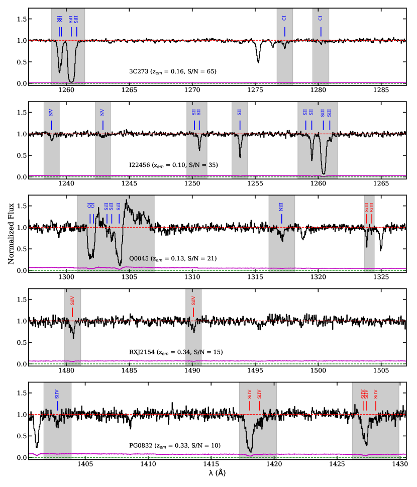
Figure 1: Illustration of our masking procedure. Different panels show random 30 Å regions of five quasar spectra with different S/N per pixel as denoted in panels, in decreasing order from top to bottom panel. The red and green dash lines indicate continuum ($y=1$ line) and zero level ($y=0$ line). Magenta curve shows the error in the normalized flux. The shaded regions show our masks. Blue and red ticks indicate the metal absorption from the ISM of the Milky Way and from intervening absorbers, respectively. We also mask geocoronal airglow emissions as shown in middle panel associated with O i ($\lambda\sim 1305$ Å).

2 Data and Masking

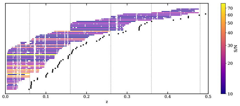
Figure 2: Redshift path covered by the Lyman-$\alpha$ forest used for our power-spectrum calculations. Horizontal lines indicate the Lyman-$\alpha$ redshift path (rest frame 1050 to 1180 Å), filled circles show the emission redshift of quasars, and vertical dashed lines demarcate the redshift bins used (i.e, 0.005-0.06, 0.06-0.16, 0.16-0.26, 0.26-0.36 and 0.36-0.48). The gaps in the horizontal lines are the masked regions of spectra (see e.g Fig. 1) containing metal lines, emission lines, spectral-gaps, and bad data. This is a subsample of spectra from Danforth et al. (2016) where the the unmasked Lyman-$\alpha$ forest has S/N (per COS pixel) $\geq 10$, as indicated with a colorbar.

We use high-quality medium-resolution ($R\sim 18000$, $\Delta v\sim 17$ km s^-1) quasar spectra obtained from HST/COS as a part of the large low-$z$ IGM survey by Danforth et al. (2016). This survey contains 82 quasar spectra at $z_{\rm em}<0.72$ observed in the wavelength range from $1130-1800$ Å, which covers the Lyman-$\alpha$ forest at $z<0.48$. The observations were obtained with the G130M and G160M gratings between year 2009 and 2013. Danforth et al. (2016) co-added individual spectra (combining both gratings whenever available), fitted continua, and identified nearly all individual absorption and emission lines. We use these continuum-fitted spectra along with the line catalog made publicly available by Danforth et al. (2016) as a high-level science product at Mikulski Archive for Space Telescopes.

To calculate the Lyman-$\alpha$ forest flux power spectrum, P$(k)$, we mask all absorption lines arising from higher Lyman series transitions than Lyman-$\alpha$, the metal lines arising from intervening systems and the interstellar medium (ISM) of the Milky Way, all emission lines including geocoronal airglow emission, low quality data having S/N $<5$ per pixel, and all gaps in the spectral coverage. To illustrate our masking procedure, we show five random chunks of spectra with different S/N in Fig. 1. The shaded regions in Fig. 1 show our masks. In the Lyman-$\alpha$ forest, masking is critical to removing metal contamination and estimating the power spectrum correctly (see, e.g, Walther et al., 2018). We discuss the effect of not masking metals on the power spectrum in Appendix A.

After masking, we restrict our further analysis to the rest-frame wavelength range between 1050 and 1180 Å in each quasar spectrum to avoid proximity zones of quasars ($\lambda>1180$ Å) and the excessive masking of data due to the presence of higher Lyman series forest lines ($\lambda<1050$Å). The redshift path covered by the unmasked Lyman-$\alpha$ forest data is shown in Fig. 2 where the quasars are ordered vertically by increasing redshift. Gaps in the horizontal lines show our masking. Vertically aligned gaps indicate masking due to strong Milky Way metal lines. A large gap at 1305 Å ($z\sim 0.07$) is due to a combination of an O i geocoronal airglow emission line and strong Si ii and O i absorption lines from the Milky Way (see e.g the middle panel of Fig. 1).

After masking and choosing the relevant wavelength range, we calculate the median S/N per pixel in the unmasked regions and impose a median S/N $>10$ (per pixel) cut to the 82 quasar spectra. Although in our power spectrum calculation we subtract the noise (see Section 3), we choose this S/N cut to ensure that we are not sensitive to systematic errors associated with how well we know the properties of the noise. Note that our S/N estimate is different than the default values provided in Danforth et al. (2016) who computed the S/N per resolution element over the entire spectrum. After applying our S/N cut, we are left with the Lyman-$\alpha$ forest of 66 quasars out of the initial 82. Individual values of this S/N per pixel are indicated in Fig. 2 via different colors.

We then split the total redshift path covered by these 66 high S/N Lyman-$\alpha$ forest spectra into five redshift bins as illustrated by the vertical dashed lines in Fig. 2 and summarized in Table 1. The first bin is chosen from $z=0.005$ to $0.06$ to remove any systematics arising from the extended wings of geocoronal Lyman-$\alpha$ emission line, which sets the lower limit of this redshift bin. The next three bins ($z=0.06-0.16$, $z=0.16-0.26$ and $z=0.26-0.36$) are chosen to have the same width ($\Delta z=0.1$) and also because the mean redshifts of the Lyman-$\alpha$ forests in these bins are nicely centered at $z=0.1,\,0.2$, and $0.3$ where we can compare our UV background measurements with previous studies (e.g Shull et al., 2015; Gaikwad et al., 2017a, b). The last redshift bin ($z=0.36-0.48$) encloses the remaining redshift-path covered by the data. Finally, in each redshift bin we removed short spectra that span less than 10% of the redshift bin-width. This criterion removes one more spectrum from the last bin and we are left with a total of 65 quasar spectra shown in Fig. 2.

Table 1: Details of the data and comparison simulation

Redshift	${\bar{z}}^{a}$	Number	Simulation	Simulation
bin		of quasars	redshift	T0 (K) and $\gamma$
0.005 - 0.06	0.03	39	0.03	5033   1.73
0.06 - 0.16	0.10	34	0.10	5288   1.72
0.16 - 0.26	0.20	19	0.20	5652   1.71
0.26 - 0.36	0.30	13	0.30	6010   1.69
0.36 - 0.48	0.41	9	0.40	6368   1.68

^aMean redshift of the unmasked Lyman-$\alpha$ forest in the bin.

3 Power Spectrum

In this section we discuss our method for measuring the power spectrum and present the measurement.

3.1 Method

Once the data are prepared, we calculate the P($k$) following the method presented in Walther et al. (2018). A brief description of the method is as follows. We first calculate the flux contrast of each spectrum in a redshift bin $\delta_{F}=(F-\bar{F})/\bar{F}$ where $\bar{F}$ is the mean flux of that spectral chunk in the bin. Then we use a Lomb-Scargle periodogram (Lomb, 1976; Scargle, 1982) to calculate the raw power spectrum $P_{\rm raw}(k)$. We subtract off the noise power $P_{\rm noise}(k)$ from $P_{\rm raw}(k)$ and divide the difference by the square of the window function $W(k,R)$ corresponding to the appropriate COS line spread function (LSF) to correct for finite resolution and pixelization (for more details see Palanque-Delabrouille et al., 2013; Walther et al., 2018). Therefore, our final power spectrum is

$$P(k)=\bigg{\langle}\,\frac{P_{\rm raw}(k)-P_{\rm noise}(k)}{W^{2}(k,R)}\,\bigg{\rangle}.$$ (1)

We use the same logarithmic binning used in Walther et al. (2018), and the average is performed over individual Lomb-Scargle periodograms of all Lyman-$\alpha$ forest chunks in each bin. We follow the standard normalization of the power spectrum, i.e. the variance in the flux contrast is $\sigma^{2}_{\delta_{F}}=\int_{-\infty}^{\infty}{dk\,P(k)/2\pi}$. The noise power within a bin is calculated using many realizations of Gaussian random noise generated from the error vector of each spectrum of the bin. For estimating the window function, we used the COS LSFs corresponding to the different gratings and lifetime positions depending on the observational parameters for each spectrum. In particular, spectra at $\bar{z}=0.2$ bin have overlapping contribution from both the G130M and the 160M grating. In this redshift bin, motivated by the co-addition routine used by Danforth et al. (2016) we take 1460 Å as the wavelength where the transition between the gratings happen.

The COS LSF is quite different from the typical Gaussian LSFs that govern ground based spectroscopic observations and exhibits broad wings. In Appendix C, we discuss the effect of incorrectly assuming a Gaussian LSF on the obtained $P(k)$ instead of using the correct non-Gaussian COS LSF. Finally, we calculate the uncertainties in P$(k)$, the diagonal elements of covariance matrix $C_{ii}\equiv\sigma_{i}^{2}$, by bootstrap resampling using $10^{4}$ random realizations of the dataset. Note that we do not have enough data to estimate the full covariance matrix $C_{ij}$. We recommend that researchers attempting to fit our power spectrum calculate the full covariance matrix by computing the correlation matrix $R_{ij}=C_{ij}/\sigma_{i}\sigma_{j}$ from their models, which can then be scaled by our diagonal elements to determine the full covariance matrix (see e.g. Walther et al., 2018, for details). Our P($k$) measurements and the diagonal elements of covariance matrix are given in Table 2.

3.2 Results

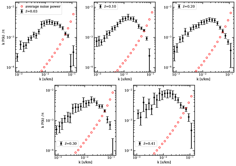
Figure 3: Our Lyman-$\alpha$ forest flux power spectrum ($k$ versus $kP(k)/\pi$) in different redshift bins (black points; see Table 1 for more details) at $k=8\times 10^{-4}$ to 0.15 s km^-1. The complete measurements are provided in Table 2. Red points show average noise power $\langle\,\frac{P_{\rm noise}(k)}{W^{2}(k,R)}\rangle$ that we subtract from raw power to obtain the power spectrum measurements (see Eq. 1). The average noise power is always less than 5% of the final power at $k<0.01$ s/km.

In Fig 3, we show our power spectrum measurement in different redshift bins, which reliably probes the power over the range $k\sim 5\times 10^{-4}$ to 0.15 s km^-1 (see Table 2). In contrast to $z>2$, the relative ease of identifying and masking metal absorption lines at these low redshifts allows us to probe the small-scale (high-$k$) power-spectrum with negligible systematics due to non-Lyman-$\alpha$ absorption. We discuss the effect of not masking metals on the power spectrum in Appendix A.

At all redshifts, our measured power spectrum shows a clear small scale cut-off at $k>0.03$ s km^-1. This cut-off is a signature of pressure smoothing and Doppler broadening of the Lyman-$\alpha$ forest. At small scales, the Lyman-$\alpha$ forest is supported by the thermal-pressure and does not follow the dark-matter density fluctuations (Hui & Gnedin, 1997; Kulkarni et al., 2015; Oñorbe et al., 2017; Rorai et al., 2017; Nasir et al., 2017). This pressure support, in addition to the Doppler broadening, smooths out the fluctuations in the Lyman-$\alpha$ forest flux and gives rise to the small-scale cut-off seen in the power spectrum (see e.g, Peeples et al., 2010; Rorai et al., 2013). This cut-off is an important feature that probes the thermal state of the IGM (Zaldarriaga et al., 2001; Walther et al., 2019).

The amplitude of the power spectra at all $k$ is significantly smaller than that obtained at high-$z$ (see, e.g, Walther et al., 2018). This is because the density evolution of the Universe results in lower overall opacity in the low-z IGM giving rise to a thinner low-z Lyman-$\alpha$ forest. This reduced opacity also reduces the power at all scales. Nevertheless, we have obtained high precision measurements (15% at $z<0.2$, 25% at $z=0.3$ and 30% at $z=0.41$ over $0.001<k<0.1$ s km^-1 scale) of the power spectrum because of the large sample size. In contrast to high-$z$, the redshift evolution of the amplitude of the power appears quite shallow. This evolution is so weak that it is challenging to identify; for example, our large scale power ($k<0.02$ s km^-1) measurement at $\bar{z}=0.2$ is only slightly lower than that at $\bar{z}=0.1$. Such non-monotonic redshift evolution is unexpected but likely results from a combination of noise fluctuations and very shallow redshift evolution. Indeed, extremely shallow evolution in the power spectrum amplitude is not unexpected at low-$z$. The power spectrum $P(k,z)\propto\langle FF^{\ast}\rangle\propto e^{-2\tau(z)}$ scales with the evolution of the optical depth $\tau(z)$. Following the fluctuating Gunn-Peterson approximation (FGPA), we can write (Gunn & Peterson, 1965; Croft et al., 1998)

$$\tau(z)\propto\,\Gamma_{\rm HI}^{-1}\,T_{0}^{-0.7}\,n_{\rm H}^{2},$$ (2)

where $\Gamma_{\rm HI}$ is the photoionization rate of H i from the UV background (UVB) and $n_{\rm H}$ is the hydrogen density. Using $\Gamma_{\rm HI}(z)\propto(1+z)^{5}$ (from Shull et al., 2015; Gaikwad et al., 2017a), $n_{\rm H}(z)\propto(1+z)^{3}$ from cosmological density evolution, and assuming a power law redshift evolution for $T_{0}(z)\propto(1+z)^{\beta}$, the opacity of the IGM should scale as $\tau\propto(1+z)^{1-0.7{\beta}}$. In the absence of any non-standard heating processes, theory predicts a cool-down of the IGM at low redshift suggesting $\beta>0$ (see e.g, Upton Sanderbeck et al., 2016). This suggests that $\tau(z)$ and the resulting amplitude of the power spectrum evolve slowly at low redshifts. However, note that the FGPA is not a good approximation for the low-$z$ IGM, at least for the power spectrum at large scales (small $k$), because it does not include the effects of shock-heated gas, as explained in Section 4 and Fig. 4. Therefore, the redshift evolution of the amplitude of the large scale power is likely to be more complicated than the simple picture presented here.

The flux power spectrum at redshifts $0.1\leq z\leq 0.4$ was also presented by Gaikwad et al. (2017a), however they split observed spectra into chunks of size 50 cMpc/h to compare with their simulation box size for the specific purpose of only evaluating the UV background. Also their method of calculating the power spectrum and the normalization is quite different from ours. For example, they fill the masks with added continuum and random noise and estimate the power spectrum of the flux ($F$) rather than the flux-contrast ($\delta F$). For these reasons, we are unable to compare with the Gaikwad et al. (2017a) power spectrum measurements directly. However, we can compare with their UV background measurements, which use not only the power-spectrum but also the flux probability density function (PDF) and column-density distribution function (CDDF; Gaikwad et al., 2017b).

Table 2: Power spectrum measurement

${\bar{z}}$	$k(s/km)$	$kP(k)/\pi$	$\sigma_{kP(k)/\pi}$	${\bar{z}}$	$k(s/km)$	$kP(k)/\pi$	$\sigma_{kP(k)/\pi}$
0.03	3.937$\times 10^{-4}$	1.874$\times 10^{-4}$	7.550$\times 10^{-5}$	0.20	2.794$\times 10^{-3}$	1.298$\times 10^{-3}$	2.129$\times 10^{-4}$
0.03	4.390$\times 10^{-4}$	1.228$\times 10^{-4}$	5.164$\times 10^{-5}$	0.20	3.551$\times 10^{-3}$	1.892$\times 10^{-3}$	2.949$\times 10^{-4}$
0.03	7.825$\times 10^{-4}$	3.137$\times 10^{-4}$	9.136$\times 10^{-5}$	0.20	4.466$\times 10^{-3}$	2.219$\times 10^{-3}$	4.231$\times 10^{-4}$
0.03	8.805$\times 10^{-4}$	2.267$\times 10^{-4}$	6.759$\times 10^{-5}$	0.20	5.636$\times 10^{-3}$	2.348$\times 10^{-3}$	3.451$\times 10^{-4}$
0.03	1.170$\times 10^{-3}$	5.812$\times 10^{-4}$	1.833$\times 10^{-4}$	0.20	7.117$\times 10^{-3}$	2.612$\times 10^{-3}$	5.248$\times 10^{-4}$
0.03	1.528$\times 10^{-3}$	5.083$\times 10^{-4}$	1.726$\times 10^{-4}$	0.20	8.969$\times 10^{-3}$	3.162$\times 10^{-3}$	5.229$\times 10^{-4}$
0.03	1.874$\times 10^{-3}$	5.534$\times 10^{-4}$	1.232$\times 10^{-4}$	0.20	1.130$\times 10^{-2}$	3.278$\times 10^{-3}$	5.957$\times 10^{-4}$
0.03	2.322$\times 10^{-3}$	8.393$\times 10^{-4}$	1.814$\times 10^{-4}$	0.20	1.420$\times 10^{-2}$	3.584$\times 10^{-3}$	6.451$\times 10^{-4}$
0.03	2.915$\times 10^{-3}$	9.651$\times 10^{-4}$	1.717$\times 10^{-4}$	0.20	1.788$\times 10^{-2}$	3.943$\times 10^{-3}$	5.999$\times 10^{-4}$
0.03	3.670$\times 10^{-3}$	1.265$\times 10^{-3}$	2.399$\times 10^{-4}$	0.20	2.255$\times 10^{-2}$	3.809$\times 10^{-3}$	5.501$\times 10^{-4}$
0.03	4.523$\times 10^{-3}$	1.161$\times 10^{-3}$	2.277$\times 10^{-4}$	0.20	2.838$\times 10^{-2}$	3.695$\times 10^{-3}$	5.647$\times 10^{-4}$
0.03	5.691$\times 10^{-3}$	1.576$\times 10^{-3}$	2.837$\times 10^{-4}$	0.20	3.576$\times 10^{-2}$	2.974$\times 10^{-3}$	4.456$\times 10^{-4}$
0.03	7.217$\times 10^{-3}$	2.721$\times 10^{-3}$	6.823$\times 10^{-4}$	0.20	4.503$\times 10^{-2}$	2.129$\times 10^{-3}$	2.573$\times 10^{-4}$
0.03	9.028$\times 10^{-3}$	2.958$\times 10^{-3}$	5.895$\times 10^{-4}$	0.20	5.667$\times 10^{-2}$	1.648$\times 10^{-3}$	2.354$\times 10^{-4}$
0.03	1.137$\times 10^{-2}$	3.248$\times 10^{-3}$	5.704$\times 10^{-4}$	0.20	7.131$\times 10^{-2}$	1.138$\times 10^{-3}$	2.070$\times 10^{-4}$
0.03	1.431$\times 10^{-2}$	3.343$\times 10^{-3}$	6.273$\times 10^{-4}$	0.20	8.975$\times 10^{-2}$	7.136$\times 10^{-4}$	1.244$\times 10^{-4}$
0.03	1.792$\times 10^{-2}$	3.142$\times 10^{-3}$	4.820$\times 10^{-4}$	0.20	1.130$\times 10^{-1}$	3.709$\times 10^{-4}$	2.719$\times 10^{-4}$
0.03	2.250$\times 10^{-2}$	2.907$\times 10^{-3}$	4.776$\times 10^{-4}$	0.30	5.576$\times 10^{-4}$	4.136$\times 10^{-4}$	2.045$\times 10^{-4}$
0.03	2.837$\times 10^{-2}$	2.966$\times 10^{-3}$	3.903$\times 10^{-4}$	0.30	8.690$\times 10^{-4}$	5.103$\times 10^{-4}$	1.624$\times 10^{-4}$
0.03	3.578$\times 10^{-2}$	2.438$\times 10^{-3}$	3.273$\times 10^{-4}$	0.30	1.126$\times 10^{-3}$	6.460$\times 10^{-4}$	2.556$\times 10^{-4}$
0.03	4.503$\times 10^{-2}$	2.045$\times 10^{-3}$	2.542$\times 10^{-4}$	0.30	1.406$\times 10^{-3}$	8.403$\times 10^{-4}$	3.366$\times 10^{-4}$
0.03	5.666$\times 10^{-2}$	1.349$\times 10^{-3}$	1.670$\times 10^{-4}$	0.30	1.786$\times 10^{-3}$	1.175$\times 10^{-3}$	3.081$\times 10^{-4}$
0.03	7.133$\times 10^{-2}$	1.137$\times 10^{-3}$	1.502$\times 10^{-4}$	0.30	2.330$\times 10^{-3}$	1.396$\times 10^{-3}$	5.073$\times 10^{-4}$
0.03	8.982$\times 10^{-2}$	1.082$\times 10^{-4}$	1.681$\times 10^{-4}$	0.30	2.846$\times 10^{-3}$	1.315$\times 10^{-3}$	4.777$\times 10^{-4}$
0.03	1.131$\times 10^{-1}$	3.235$\times 10^{-4}$	2.101$\times 10^{-4}$	0.30	3.575$\times 10^{-3}$	2.593$\times 10^{-3}$	9.301$\times 10^{-4}$
0.10	2.397$\times 10^{-4}$	2.721$\times 10^{-4}$	1.521$\times 10^{-4}$	0.30	4.537$\times 10^{-3}$	2.771$\times 10^{-3}$	9.136$\times 10^{-4}$
0.10	2.861$\times 10^{-4}$	1.436$\times 10^{-4}$	4.891$\times 10^{-5}$	0.30	5.706$\times 10^{-3}$	2.767$\times 10^{-3}$	7.532$\times 10^{-4}$
0.10	3.521$\times 10^{-4}$	1.093$\times 10^{-4}$	5.191$\times 10^{-5}$	0.30	7.137$\times 10^{-3}$	2.966$\times 10^{-3}$	7.580$\times 10^{-4}$
0.10	4.724$\times 10^{-4}$	5.567$\times 10^{-4}$	4.046$\times 10^{-4}$	0.30	8.992$\times 10^{-3}$	4.268$\times 10^{-3}$	1.529$\times 10^{-3}$
0.10	5.742$\times 10^{-4}$	3.166$\times 10^{-4}$	8.959$\times 10^{-5}$	0.30	1.131$\times 10^{-2}$	3.695$\times 10^{-3}$	9.241$\times 10^{-4}$
0.10	7.142$\times 10^{-4}$	3.239$\times 10^{-4}$	1.059$\times 10^{-4}$	0.30	1.424$\times 10^{-2}$	3.936$\times 10^{-3}$	8.243$\times 10^{-4}$
0.10	9.321$\times 10^{-4}$	7.483$\times 10^{-4}$	2.526$\times 10^{-4}$	0.30	1.793$\times 10^{-2}$	5.021$\times 10^{-3}$	1.199$\times 10^{-3}$
0.10	1.139$\times 10^{-3}$	8.075$\times 10^{-4}$	2.949$\times 10^{-4}$	0.30	2.256$\times 10^{-2}$	4.804$\times 10^{-3}$	7.301$\times 10^{-4}$
0.10	1.417$\times 10^{-3}$	6.968$\times 10^{-4}$	1.449$\times 10^{-4}$	0.30	2.842$\times 10^{-2}$	3.819$\times 10^{-3}$	6.866$\times 10^{-4}$
0.10	1.812$\times 10^{-3}$	9.472$\times 10^{-4}$	2.221$\times 10^{-4}$	0.30	3.576$\times 10^{-2}$	2.999$\times 10^{-3}$	4.241$\times 10^{-4}$
0.10	2.265$\times 10^{-3}$	1.291$\times 10^{-3}$	3.512$\times 10^{-4}$	0.30	4.499$\times 10^{-2}$	2.994$\times 10^{-3}$	3.940$\times 10^{-4}$
0.10	2.841$\times 10^{-3}$	1.423$\times 10^{-3}$	2.675$\times 10^{-4}$	0.30	5.664$\times 10^{-2}$	2.110$\times 10^{-3}$	2.131$\times 10^{-4}$
0.10	3.590$\times 10^{-3}$	1.917$\times 10^{-3}$	3.613$\times 10^{-4}$	0.30	7.130$\times 10^{-2}$	1.101$\times 10^{-3}$	2.666$\times 10^{-4}$
0.10	4.511$\times 10^{-3}$	2.127$\times 10^{-3}$	3.669$\times 10^{-4}$	0.30	8.975$\times 10^{-2}$	7.149$\times 10^{-4}$	2.101$\times 10^{-4}$
0.10	5.677$\times 10^{-3}$	2.735$\times 10^{-3}$	4.798$\times 10^{-4}$	0.41	1.118$\times 10^{-3}$	1.717$\times 10^{-3}$	5.549$\times 10^{-4}$
0.10	7.151$\times 10^{-3}$	3.390$\times 10^{-3}$	5.174$\times 10^{-4}$	0.41	1.395$\times 10^{-3}$	1.287$\times 10^{-3}$	5.887$\times 10^{-4}$
0.10	8.990$\times 10^{-3}$	4.109$\times 10^{-3}$	7.895$\times 10^{-4}$	0.41	1.801$\times 10^{-3}$	3.991$\times 10^{-3}$	2.017$\times 10^{-3}$
0.10	1.130$\times 10^{-2}$	4.269$\times 10^{-3}$	6.702$\times 10^{-4}$	0.41	2.259$\times 10^{-3}$	2.333$\times 10^{-3}$	1.102$\times 10^{-3}$
0.10	1.423$\times 10^{-2}$	4.864$\times 10^{-3}$	1.069$\times 10^{-3}$	0.41	2.870$\times 10^{-3}$	3.762$\times 10^{-3}$	1.463$\times 10^{-3}$
0.10	1.792$\times 10^{-2}$	4.292$\times 10^{-3}$	5.291$\times 10^{-4}$	0.41	3.616$\times 10^{-3}$	2.445$\times 10^{-3}$	8.784$\times 10^{-4}$
0.10	2.255$\times 10^{-2}$	4.104$\times 10^{-3}$	7.505$\times 10^{-4}$	0.41	4.516$\times 10^{-3}$	5.841$\times 10^{-3}$	2.415$\times 10^{-3}$
0.10	2.839$\times 10^{-2}$	3.489$\times 10^{-3}$	3.827$\times 10^{-4}$	0.41	5.687$\times 10^{-3}$	4.887$\times 10^{-3}$	2.170$\times 10^{-3}$
0.10	3.573$\times 10^{-2}$	2.375$\times 10^{-3}$	3.648$\times 10^{-4}$	0.41	7.172$\times 10^{-3}$	8.052$\times 10^{-3}$	3.469$\times 10^{-3}$
0.10	4.497$\times 10^{-2}$	2.027$\times 10^{-3}$	2.117$\times 10^{-4}$	0.41	9.012$\times 10^{-3}$	7.250$\times 10^{-3}$	2.318$\times 10^{-3}$
0.10	5.663$\times 10^{-2}$	1.736$\times 10^{-3}$	1.238$\times 10^{-4}$	0.41	1.133$\times 10^{-2}$	7.995$\times 10^{-3}$	1.968$\times 10^{-3}$
0.10	7.131$\times 10^{-2}$	9.309$\times 10^{-4}$	1.217$\times 10^{-4}$	0.41	1.427$\times 10^{-2}$	8.106$\times 10^{-3}$	2.493$\times 10^{-3}$
0.10	8.977$\times 10^{-2}$	2.450$\times 10^{-4}$	1.744$\times 10^{-4}$	0.41	1.793$\times 10^{-2}$	8.183$\times 10^{-3}$	2.148$\times 10^{-3}$
0.20	2.666$\times 10^{-4}$	9.025$\times 10^{-5}$	2.044$\times 10^{-5}$	0.41	2.252$\times 10^{-2}$	7.539$\times 10^{-3}$	2.298$\times 10^{-3}$
0.20	5.359$\times 10^{-4}$	2.741$\times 10^{-4}$	8.676$\times 10^{-5}$	0.41	2.835$\times 10^{-2}$	6.100$\times 10^{-3}$	1.462$\times 10^{-3}$
0.20	7.364$\times 10^{-4}$	1.893$\times 10^{-4}$	5.990$\times 10^{-5}$	0.41	3.576$\times 10^{-2}$	4.826$\times 10^{-3}$	9.621$\times 10^{-4}$
0.20	8.586$\times 10^{-4}$	3.430$\times 10^{-4}$	1.778$\times 10^{-4}$	0.41	4.502$\times 10^{-2}$	3.285$\times 10^{-3}$	6.987$\times 10^{-4}$
0.20	1.078$\times 10^{-3}$	4.733$\times 10^{-4}$	1.528$\times 10^{-4}$	0.41	5.666$\times 10^{-2}$	2.789$\times 10^{-3}$	2.951$\times 10^{-4}$
0.20	1.394$\times 10^{-3}$	8.696$\times 10^{-4}$	1.969$\times 10^{-4}$	0.41	7.131$\times 10^{-2}$	2.367$\times 10^{-3}$	3.749$\times 10^{-4}$
0.20	1.767$\times 10^{-3}$	9.598$\times 10^{-4}$	2.439$\times 10^{-4}$	0.41	8.977$\times 10^{-2}$	1.319$\times 10^{-3}$	3.876$\times 10^{-4}$
0.20	2.200$\times 10^{-3}$	1.607$\times 10^{-3}$	4.047$\times 10^{-4}$	0.41	1.131$\times 10^{-1}$	4.726$\times 10^{-4}$	3.530$\times 10^{-4}$

A machine readable version is available on ArXiv ancillary files and on MNRAS webpage.

4 Implications for the UV background

The amplitude of the Lyman-$\alpha$ forest power spectrum is sensitive to the UV background; therefore, it can be used to measure the UV background quantified by the H i photoionization rate $\Gamma_{{\mbox{\scriptsize H$\,${\sc i}}}}$. The basic idea behind the measurement is to compare the power-spectrum with cosmological hydrodynamical simulations of the IGM where $\Gamma_{{\mbox{\scriptsize H$\,${\sc i}}}}$ is one of the free parameters. In this section, we first discuss our IGM simulations and then the $\Gamma_{{\mbox{\scriptsize H$\,${\sc i}}}}$ measurements obtained from them.

4.1 Simulations

For comparing our power spectrum measurements with the simulated IGM, we ran an Nyx cosmological hydrodynamic simulation (Almgren et al., 2013; Lukić et al., 2015) from $z=159$ to $z=0.03$. This is an Eulerian hydrodynamical simulation of box size 20 cMpc/h and 1024³ cells. The initial conditions were generated using MUSIC code (Hahn & Abel, 2011) along with the transfer function from CAMB (Lewis et al., 2000; Howlett et al., 2012). We evolve baryon hydrodynamics in Eulerian approach on a fixed Cartesian grid with 1024³ cells, and follow the evolution of dark matter using 1024³ Lagrangian (N-body) particles. This simulation resolves 19.5 ckpc/h scales (i.e, $\Delta v<2$ km s^-1 at $z<0.5$). In this simulation, we used the photoheating rates from the Puchwein et al. (2019) non-equilibrium models (the equivalent-equilibrium rates since our code assumes ionization equilibrium). We stored simulation outputs at different redshifts corresponding to our $\bar{z}$ at the measured P($k$). We determined T₀ and $\gamma$ by fitting the distribution of densities and temperatures in the simulation following the linear least squares method described in Lukić et al. (2015). The simulation redshifts, T₀, and $\gamma$ are provided in Table 1. The values of T₀ and $\gamma$ are also consistent with the theoretical models presented in McQuinn (2016) and obtained in the simulations presented by Shull et al. (2015) and Gaikwad et al. (2017a).

For our current purposes, the only free parameter in this simulation is $\Gamma_{\rm H\,I}$. We vary $\Gamma_{\rm H\,I}$ and generate the simulated Lyman-$\alpha$ forest as follows. First, we calculate the ionization fractions of hydrogen and helium under the assumption of ionization equilibrium including both photoionization and collisional ionization. For this we have used updated cross-sections and recombination rates from Lukić et al. (2015). Then, we extract a large number ($5\times 10^{4}$) of random lines-of-sight (skewers) parallel to the (arbitrarily chosen) $z-$axis of the simulation cube. Along these lines-of-sight, we store the ionization densities, temperatures and $z$-component of the velocities. As our procedure does not include radiative transfer, we model the self-shielding of dense cells using the prescription described in Rahmati et al. (2013). We generate the simulated Lyman-$\alpha$ optical depth for each cell along the line of sight, which we will refer to as $\tau$-skewers, by summing all the real space contributions to the redshift space optical depth using the full Voigt profile resulting from each (real-space) cell following the approximations used in Tepper-García (2006). The flux $F=e^{-\tau}$ gives us the continuum normalized Lyman-$\alpha$ forest flux along these skewers. These constitute our ‘perfect skewers’ from the simulation. We calculate and store 5$\times$10⁴ simulated skewers from each box for different values of $\Gamma_{\rm H\,I}$.

Note that every-time we change the $\Gamma_{\rm H\,I}$ we recalculate the skewers following the procedure described above. We do not simply rescale the $\tau$ values along the skewers when we change the $\Gamma_{\rm H\,I}$, as is typically applied to simulations of the Lyman-$\alpha$ forest at higher redshifts following the FGPA. According to the FGPA, $\tau\propto\Gamma_{\rm H\,I}^{-1}$ (from Eq. 2), which is a good approximation at high-$z$ when most of the gas in the IGM is photoionized. However, a large amount of gas in the low-$z$ Universe is collisionally ionized because it is heated to $T>10^{5}\,{\rm K}$ by structure formation shocks (see Davé et al., 2010; Shull et al., 2012). In this regime, the simple rescaling of $\tau$ following the FGPA leads to erroneous results, because the contribution of collisional ionization implies that the true optical depth is no longer linearly proportional to $\Gamma_{\rm H\,I}$ (see also Lukić et al., 2015). This is illustrated in Fig. 4 where we show the power-spectrum for $\tau$-skewers generated with a fiducial value of $\Gamma_{\rm H\,I\,Fid}=1.75\times 10^{-13}$ s^-1 (black-curve) and three more power-spectra where the $\tau$-skewers were initially calculated for $\Gamma_{\rm H\,I\,Fid}\times 4$, $\Gamma_{\rm H\,I\,Fid}/3.5$ and $\Gamma_{\rm H\,I,Fid}/2$ values and then rescaled to get the $\tau$-skewers corresponding to $\Gamma_{\rm H\,I\,Fid}$ following FGPA. The latter three deviate significantly from the fiducial power-spectrum on large scales (low $k<0.04$ s km^-1values). The bottom panel of Fig. 4 shows the percentage differences in the correct calculation versus the ones obtained by using the FGPA. The differences are large (of the order of 10 to 25%) when the FGPA is applied for larger difference in $\Gamma_{\rm H\,I}$ (of factor 2 to 4). Given that the reported low-$z$ $\Gamma_{\rm H\,I}$ measurements vary over factors of $2-5$, the results obtained by incorrectly using FGPA can give large systematic differences in the derived $\Gamma_{\rm H\,I}$ values.

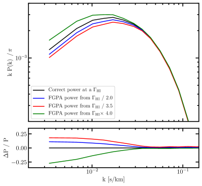
Figure 4: The effect of using the FGPA on power-spectra. Top panel shows $z=0.2$ power-spectrum estimated for $\Gamma_{\rm H\,I\,Fid}=1.75\times 10^{-13}$ s^-1 (black-curve) by correctly calculating the $\tau$-skewers. The green, blue and red curves show power-spectra estimated when $\tau$-skewers, which were initially calculated for $\Gamma_{\rm H\,I\,Fid}\times 4$, $\Gamma_{\rm H\,I}/2$ and $\Gamma_{\rm H\,I\,Fid}/3.5$ values, were rescaled to $\Gamma_{\rm H\,I\,Fid}$ values by following FGPA. At $k<0.04$ s km^-1 the power-spectra obtained using FGPA deviates from the correct power-spectrum (black-curve) and the percentage deviation are shown in the bottom panel with the same colors. The deviation is large for large differences in the initial and final $\Gamma_{\rm H\,I}$ values.

Once the perfect-skewers are constructed, we adopt a forward modeling approach to make them look like realistic spectra. To this end, we follow the procedure developed in Walther et al. (2018) but for the HST COS data. We first stitch randomly drawn skewers together to cover the Lyman-$\alpha$ forest redshift path of each quasar. Then, we convolve these skewers with the finite COS LSFs corresponding to the same gratings and lifetime positions as the data for each quasar. Then, we rebin these to match the pixels of the actual data, and we add Gaussian random noise at each pixel generated with the standard deviation of the error-vector from the observed spectra. Finally, we mask these spectra in exactly same manner as the data and follow the same procedure to calculate the power-spectrum (see Section 3.1). We calculate $P(k)$ from these forward models created for a large number of $\Gamma_{\rm H\,I}$ values and estimate the $\Gamma_{\rm H\,I}$ by comparing with the $P(k)$ measurements as explained in the next sub-section.

4.2 Constraints on the UV background

The power spectrum is not only sensitive to $\Gamma_{\rm H\,I}$ but also to the thermal state of the IGM quantified by $T_{0}$ and $\gamma$. Therefore, to correctly measure the $\Gamma_{\rm H\,I}$ using our power spectrum, we need a large ensemble of simulations of different IGM thermal state models stored at the redshifts where we have measured the power spectrum. We have the THERMAL grid (Hiss et al., 2018; Walther et al., 2019) available with $>70$ Nyx simulations (with box size 20 cMpc/h and 1024³ particles) of different IGM thermal models but only a single redshift $z=0.2$ overlaps with our dataset presented here. We use 50 simulations from this suite and follow the Bayesian inference approach presented in Walther et al. (2019), where the likelihood of the model is given by

$$\mathcal{L}\equiv P(\mathrm{data}|\mathrm{model})$$ (3)

$$\propto \prod_{\mathrm{datasets}}\frac{1}{\sqrt{\det(C)}}\exp\left(-\frac{\mathbf{\Delta}^{\mathrm{T}}C^{-1}\mathbf{\Delta}}{2}\right)$$

$$\mathbf{\Delta}= \mathbf{P}_{\mathrm{data}}-\mathbf{P}_{\mathrm{model}}$$

Here $C$ is the covariance matrix of the measurements where the diagonal elements are taken from the uncertainties obtained here (see Table 2), and the off-diagonal elements are estimated from the forward model which is closest in the parameter space to the model in question. Using this $\mathcal{L}$, we perform a Bayesian inference at $z=0.2$ using Markov Chain Monte Carlo methods (MCMC) and jointly estimate the $T_{0}$, $\gamma$, and $\Gamma_{\rm H\,I}$ at $z=0.2$ (Walther et al. in prep.). We then marginalize the joint posterior distribution over parameters $T_{0}$ and $\gamma$ to determine $\Gamma_{\rm H\,I}$ and its 68% confidence interval.

At other redshifts, we do not yet have such a large simulation grid. However the analysis at $z=0.2$ provides a clear indication of how much the degeneracies in the thermal state of the low-z IGM propagate into uncertainties on the $\Gamma_{\rm H\,I}$ measurements. To estimate the $\Gamma_{\rm H\,I}$ at other redshifts but using only one thermal model rather than a large grid of thermal models, we simply assume that the scaling between uncertainties at these redshifts behave similarly to our $z=0.2$ $\Gamma_{\rm H\,I}$ measurement. To quantify the amount by which the uncertainties on the $\Gamma_{\rm H\,I}$ can be underestimated if one uses only a single simulation instead of the full grid, we repeat the analysis mentioned above at $z=0.2$ but using only one simulation with $\Gamma_{\rm H\,I}$ being the only free parameter. In this analysis, we are using the same simulation for which we have stored outputs at other redshifts as well (as described in Section 3 and Table 1). Also, for this $\Gamma_{\rm HI}$ estimate, we opt to use only the diagonal elements of the covariance matrix because the shape of power spectrum does not vary widely in this single parameter model where the IGM thermal state is fixed. We found that fitting with the full covariance led to spurious bad fits resulting from the rigidity of the model of the power spectrum shape if the thermal state is fixed. In this case, where we use only one simulation (and hence one thermal model) and the diagonal elements of covariances, we calculate the $\Gamma_{\rm H\,I}$ and its uncertainties represented by 68% confidence intervals by performing a maximum likelihood analysis. We find that these uncertainties are underestimated by a factor of 5.75 as compared to the one obtained using full simulation grid and covariances.

We repeat this calculation at other redshifts and obtain the $\Gamma_{\rm H\,I}$ and the 68% confidence interval using only the diagonal elements. Next, we multiply this confidence interval by factor of 5.75 so that it correctly represents the uncertainties arising from degeneracies in the thermal state of the low-$z$ IGM. We believe that this approach of obtaining uncertainties at redshifts other than $z=0.2$, although approximate, is nevertheless a significant improvement over previous estimates of $\Gamma_{\rm H\,I}$ that are based on IGM simulation outputs which effectively assume perfect knowledge of the thermal state of the IGM. Nevertheless, in a companion paper (Walther et al. in prep.), we will present joint constraints on $T_{0}$, $\gamma$, and $\Gamma_{\rm H\,I}$. For all $\Gamma_{\rm H\,I}$ estimates discussed here, we have fit our power spectrum measurements over the range $0.03<k<0.1$ s km^-1, where the smallest $k$ is chosen to minimize the box size effects and largest $k$ corresponds to scales where we have reliable uncertainties on the power spectrum measurements. However, note that our results are not sensitive to the choice of the smallest $k$ value ($k_{\rm min}$) as long as $0.03>k_{\rm min}>0.01$ s km^-1.

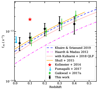
Figure 5: Our estimated $\Gamma_{\rm H\,I}$ values (black circles) compared with previous measurements by Gaikwad et al. (2017a, green diamonds), Kollmeier et al. (2014, red star), a fitting form by Shull et al. (2015, orange curve) and upper limits from Fumagalli et al. (2017, downward arrow). Prediction from a new UV background model of Khaire & Srianand (2019, blue-dash curve) is consistent with our measurements. Also, the UV background predictions using updated QLF from Kulkarni et al. (2018, red dotted curve) give consistent results with the measurements (see Section 4.2 for more details). The UV background from Haardt & Madau (2012, magenta dot-dash curve) is factor of $\sim 2$ smaller than the measurements.

Table 3: $\Gamma_{\rm H\ I}$ measurements

${\bar{z}}$	$\Gamma_{\rm H\ I}$ (10-13s-1)
0.03	0.585 ${}^{+0.17}_{-0.18}$
0.10	0.756 ${}^{+0.17}_{-0.18}$
0.20	1.135 ${}^{+0.32}_{-0.32}$
0.30	1.479 ${}^{+0.44}_{-0.52}$
0.41	1.418 ${}^{+0.53}_{-0.57}$

Our $\Gamma_{\rm H\,I}$ measurements and the 68% confidence interval on them obtained following the method mentioned above are provided in Table 3 and shown in Fig. 5. We also show the previous measurements reported in the literature at $z<0.5$ for comparison (however, see Davé & Tripp, 2001, for an early attempt). The upper limit at $z\sim 0$ by Fumagalli et al. (2017) was obtained from the H$\alpha$ and 21-cm observations of a nearby galaxy. All other measurements have used the Lyman-$\alpha$ forest from Danforth et al. (2016). The measurement by Kollmeier et al. (2014) at $z\sim 0.1$ and the fit resulting from the analysis by Shull et al. (2015) at $z<0.5$ were obtained by modeling the CDDF, whereas measurements of Gaikwad et al. (2017a) were obtained using the flux PDF and power-spectrum (and later confirmed with the CDDF in Gaikwad et al. 2017b). Our measurements are consistent with the previous studies except for Kollmeier et al. (2014), which is $\sim 2.5$ times higher. As compared to previous studies, we have independent measurements obtained only from the Lyman-$\alpha$ forest power spectrum extending down to $z=0.03$.

In Fig. 5, we also show predictions from the UV background models by Haardt & Madau (2012) and Khaire & Srianand (2019). Ours as well as the other $\Gamma_{\rm H\,I}$ measurements (except for Kollmeier et al., 2014) are consistent with the Khaire & Srianand (2019) UV background and are a factor of $\sim 2$ higher than Haardt & Madau (2012). The Khaire & Srianand (2019) UV background at $z<0.5$ is mostly contributed by quasars since it has been obtained with a negligible contribution from galaxies (at $z<2$; see their Eq. 13). Therefore, we argue that quasar emission is sufficient to produce the low-z UV background (Khaire & Srianand, 2015a, see also). The factor of five discrepancy between the measurement from Kollmeier et al. (2014) and the prediction from Haardt & Madau (2012) was argued to represent a photon-underproduction crisis at low-$z$. Soon after the Kollmeier et al. (2014) study, Khaire & Srianand (2015a) showed that the UV background models that include an updated quasar emissivity predict a factor of two higher $\Gamma_{\rm H\,I}$, without requiring any additional contribution from galaxies. This model later turned out to be consistent with many new $\Gamma_{\rm H\,I}$ measurements (Shull et al., 2015; Gaikwad et al., 2017a, b; Gurvich et al., 2017; Viel et al., 2017; Fumagalli et al., 2017). As shown in Fig 5, this is also consistent with our new measurements. Other recent updates to UV background models (Madau & Haardt, 2015; Khaire & Srianand, 2019; Puchwein et al., 2019) also came to the same conclusion using more recent estimates for the quasar emissivity similar to Khaire & Srianand (2015a).

Recently, Kulkarni et al. (2018) updated the fits to the quasar luminosity functions (QLF) and emissivity across a large redshift range and claim that the quasar contribution to the low-$z$ UV background is factor of $\sim 2$ smaller than the predictions by these recent UV background models (Madau & Haardt, 2015; Khaire & Srianand, 2019; Puchwein et al., 2019) and most of the measurements. However, the Kulkarni et al. (2018) calculation uses the CDDF of the IGM from tabulated fits by Haardt & Madau (2012) and an ionizing spectral slope of quasars $f_{\nu}\propto\nu^{-1.7}$ (Lusso et al., 2015). Instead, using the Inoue et al. (2014) CDDF results in a 40-60% higher UV background at $z<0.5$ (see, for e.g., Figure 16 of Gaikwad et al., 2017a). This along with including the recombination emissivities in the UV background calculations should easily increase the $\Gamma_{\rm H\,I}$ estimates of Kulkarni et al. (2018) by factor of $\sim 1.8$ as shown in Fig. 5. For this calculation we used the UV background code presented in Khaire & Srianand (2019) but with the updated quasar emissivity determined by Kulkarni et al. (2018), with the same limiting magnitude at 1450 Å ($M_{\rm 1450,lim}=-18$) and the same spectral slope $f_{\nu}\propto\nu^{-1.7}$ that they adopted, but using the Inoue et al. (2014) CDDF instead of the Haardt & Madau (2012) fits used by Kulkarni et al. (2018). We note that adopting a flatter spectral slope for quasars can further increase the $\Gamma_{\rm H\,I}$. For example, redoing the calculation mentioned above using the Kulkarni et al. (2018) emissivity and the Khaire & Srianand (2019) UV background model, but changing the quasar spectra slope to $f_{\nu}\propto\nu^{-1.4}$ consistent with the harder slope measured by Shull et al. (2012) and Stevans et al. (2014), results in a further increase of the $\Gamma_{\rm H\,I}$ by a factor of 1.3.

Finally, note that even if the $\Gamma_{\rm H\,I}$ is as high as that purported by Kollmeier et al. (2014), there is no crisis associated with photon production since a negligible contribution from galaxies, along with updated cosmic star formation histories (Madau & Dickinson, 2014; Khaire & Srianand, 2015b), can easily reproduce such a large $\Gamma_{\rm H\,I}$ (see for more details Khaire & Srianand, 2015a).

5 Summary and conclusions

We present a new high precision high resolution power spectrum measurement in five different redshift bins at $z<0.5$. For this measurement, we have used high-quality medium resolution Lyman-$\alpha$ forest data from HST/COS from the largest low-$z$ IGM survey published by Danforth et al. (2016). We applied the procedure developed in Walther et al. (2018), which takes into account masked metal-line absorptions, noise in the data and the finite resolution of the instrument. The data allow us to reliably probe the power spectrum up to small scales $k<0.1$ s km^-1 and our measurements show the expected thermal cut-off in the power at small scales $k>0.03$ s km^-1, resulting from pressure smoothing of IGM gas and thermal Doppler broadening of absorption lines. Our power spectrum measurements are provided in Table 2.

We compare these with cosmological hydrodynamical simulations and obtain constraints of the UV background at $z<0.5$. Our measured hydrogen photoionization rates (Table 3) are consistent with the previous estimates (Shull et al., 2015; Gaikwad et al., 2017a, b; Fumagalli et al., 2017) and recent UV background models (Khaire & Srianand, 2019; Puchwein et al., 2019). This suggests that the low-$z$ UV background is dominated by ionizing photons emitted by quasars without requiring any significant contribution from galaxies.

The power-spectrum measurements presented here, in principle, can probe the thermal state of the low-$z$ IGM. At low-$z$, theoretical calculations using standard heating and cooling rates show that the IGM loses memory of the previous heating episodes caused by the hydrogen and helium reionization. This makes understanding and predicting the structure of the low-$z$ IGM relatively simple, as it is independent of the physics associated with hydrogen and helium reionization heating, which complicate modeling at higher redshifts ($z\gtrsim 2$). In the absence of any other heating processes, theory predicts that the diffuse low-density photoionized IGM cools down after $z\sim 2$ and asymptotes toward a single temperature-density relation with $\gamma$ close to 1.6 and T${}_{0}\sim 5000$ K (McQuinn, 2016) at $z=0$. Such a predicted cool-down of the IGM at low-$z$ has not yet been observationally confirmed. Indeed, there are no reliable measurements of the thermal state of the IGM at $z<1.6$ (but see Ricotti & Shull, 2000) where the atmospheric cut-off does not allow us to observe Lyman-$\alpha$ forest from ground based telescopes.

In a companion paper (Walther et al. in prep.) we will use the power spectrum measurements presented here to jointly constrain the IGM thermal state (T₀, $\gamma$) and the UV background ($\Gamma_{\rm H\,I}$). These measurements will help us understand the physics of IGM and address important questions such as whether feedback processes associated with galaxy formation modify the thermal state of the IGM at low-$z$ (Viel et al., 2017; Nasir et al., 2017) and/or if there is any room for the existence of non-standard heating processes powered by TeV Blazars (Puchwein et al., 2012; Lamberts et al., 2015) or decaying dark matter (Furlanetto et al., 2006; Araya & Padilla, 2014).

In contrast with the high-$z$ Universe, the much lower opacity of Lyman series absorption arising in the low-$z$ IGM results in dramatically reduced line blanketing, making it relatively straightforward to identify all lines as either resulting from the Lyman-series or metal absorption. This results in a large redshift path length where Lyman series absorption can be studied, data analysis and preparation are simplified, and important systematics from metal-line contamination arising at small-scales (high-$k$; see section 4.1 of Walther et al., 2018) are mitigated. Furthermore, our measurements demonstrate that COS resolution is sufficient to obtain high-quality power-spectrum measurements even at the small-scales (high-$k$, $k\sim 0.1\,{\rm s\,km^{-1}}$) required for probing the thermal state of the IGM and demonstrate the important role that HST/UV spectroscopy can play in our understanding of the low-$z$ IGM. We conclude by noting that, owing to the paucity of archival near-UV spectra covering the Lyman-$\alpha$ transition at $0.5<z<1.6$, there are essentially no constraints on the physical state of IGM gas in this redshift interval, representing 5 Gyr of the Universe’s history. It is critical that HST UV spectroscopy fill this gap in our understanding of the Universe before HST’s mission is complete, otherwise we could remain in the dark for decades.

Appendix A Power spectrum without masking metal absorption lines

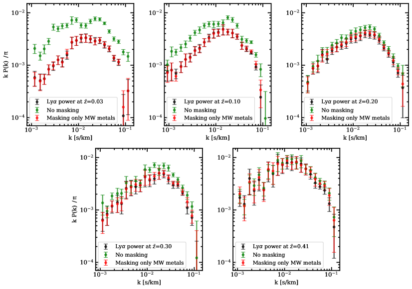
Figure 6: Illustrating the effect of masking different metal lines on the power spectrum. Black points show our power spectrum measurements as also shown in Fig. 3. Power without masking any metals (green points) is systematically higher at all scales. At lower-$z$, difference arises mainly because of Milky-way metals. This is illustrated by power spectrum shown in red points which is obtained by masking only the Milky-way metals. A small difference between red and black points shows the effect of masking intervening metals. The intervening metals have insignificant impact on the Lyman-$\alpha$ power spectrum at low-$z$. On the other hand, Milky-way metal lines are easy to identify which makes any incompleteness in intervening metal identification unimportant for calculating the power spectrum.

While preparing data for the power spectrum calculation, we have properly masked the metal lines originating from Milky-way and intervening metals as well as other contaminations (see Section 2). This is an important procedure to correctly calculate the power spectrum. However, to estimate the relevance of different metal contamination, in Fig. 6 we show the power spectrum calculated without masking any metal absorption lines (green points) and masking only Milky-way metal lines (red points) in the Lyman-$\alpha$ forest. However, note that we mask the spectral gaps and all other emission lines, which appear mainly in our lowest redshift bin ($\bar{z}=0.03$). As expected, when metal lines are not masked the power is systematically higher because of the extra fluctuations in the flux introduced by metal lines. However the difference in power is larger at lower redshift mostly because of strong metal contamination arising from the ISM of the Milky-way and many of the absorption lines are correlated as they originate from the same source and with same wavelength separation. The intervening metals have insignificant impact on the Lyman-$\alpha$ power spectrum at low-$z$ (the difference between red and black points in Fig 6). On the other hand, Milky-way metal lines are easy to identify which makes any incompleteness in intervening metal identification unimportant for calculating the power spectrum.

Appendix B Effect of masking on the power-spectrum

To check if the spectral masking is introducing any significant contamination in the power-spectrum we calculate the power spectrum from our forward models (using $\Gamma_{\rm H\,I}$ values consistent with our measurements) but without using any masking on the Lyman-$\alpha$ forest. In these forward models for the purpose of only studying the effect of masking, we are using infinite resolution noiseless spectra. In Fig. 7 we compare the resulting power spectrum with and without masking the Lyman-$\alpha$ forest. The bottom panel shows a fractional difference between these. The maximum change in relevant $k<0.1$ s km^-1 values is no more than 5% at any redshift. For comparing with the actual uncertainties in the power spectrum, we also plot the fractional errors in the bottom panel. The figure clearly shows that the fractional change in the power-spectrum because of masking is less than the errors on the actual power spectrum measurements. This motivates us not to perform the masking corrections on the measurements as done in Walther et al. (2018).

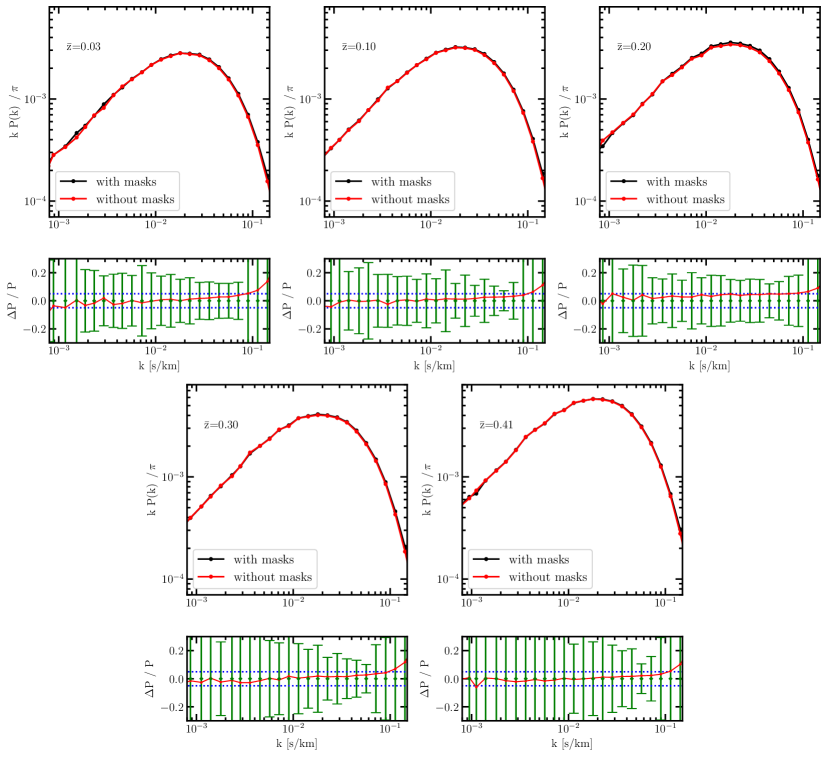
Figure 7: Effect of masking on the power spectrum. We use mock spectra generated from our forward models (infinite signal and resolution) and calculate the power spectrum for two cases. First by applying exactly same masks as in data to the forward model spectra (black-curves) and second where no masks are applied (red curves). The both curves match with each other with $<5\%$ difference as shown in the bottom panels where 5% change is marked with blue dotted line. The green error-bars show out fractional errors from the measurements. The difference is small enough to ignore and opt out of the masking correction.

Appendix C Effect of the COS LSF on the power-spectrum

The COS LSF is quite different from a Gaussian as it exhibits strong non-Gaussian wings. In the power spectrum calculation the LSF appears in the window function correction (see Eq. 1) and it is also important to generate the forward models. To see how much the power spectrum can be affected if one uses a Gaussian LSF with a similar resolution to COS we perform the following analysis. We use mock spectra generated from our forward models (at $\Gamma_{\rm H\,I}$ values consistent with our measurements) generated using the correct COS LSF but while calculating the power spectrum we use a Gaussian LSF. The resulting power spectrum (red curves) is shown in the Fig 8 along with that obtained by using the correct COS LSF (black curves). The amplitude of the power spectrum in the former is smaller at large $k$ values and the differences, as shown in the bottom panels, can be as large as 80%. This is much too large as compared to the actual uncertainties from our measurements. Although the differences decrease at higher redshifts, because of small sample sizes, the discrepancy is too significant to ignore. This exercise shows that it is never a sound choice to approximate the COS LSF as a Gaussian.

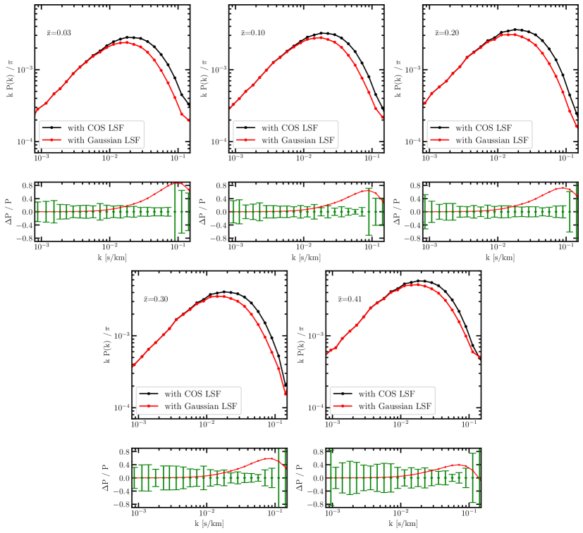
Figure 8: Effect on the power spectrum of incorrectly using the Gaussian LSF instead of COS LSF that has broad non-Gaussian wings. We use our forward models generated using the COS LSF and calculate the power spectrum with a Gaussian approximated to the COS LSF (red curves). This power spectrum is compared with that calculated using correct COS LSF (black curves). The bottom panels show the percentage difference between these compared with the fractional errors estimated from our measurements. The differences are too large to ignore. Therefore, it is never recommended to approximate the COS LSF with a Gaussian, at least for power spectrum calculations.

References

- Almgren et al. (2013) Almgren A. S., Bell J. B., Lijewski M. J., Lukić Z., Van Andel E., 2013, ApJ, 765, 39
- Araya & Padilla (2014) Araya I. J., Padilla N. D., 2014, MNRAS, 445, 850
- Becker et al. (2011) Becker G. D., Bolton J. S., Haehnelt M. G., Sargent W. L. W., 2011, MNRAS, 410, 1096
- Bolton et al. (2012) Bolton J. S., Becker G. D., Raskutti S., Wyithe J. S. B., Haehnelt M. G., Sargent W. L. W., 2012, MNRAS, 419, 2880
- Borthakur et al. (2015) Borthakur S., et al., 2015, ApJ, 813, 46
- Burchett et al. (2015) Burchett J. N., et al., 2015, ApJ, 815, 91
- Croft et al. (1998) Croft R. A. C., Weinberg D. H., Katz N., Hernquist L., 1998, ApJ, 495, 44
- Croft et al. (2002) Croft R. A. C., Weinberg D. H., Bolte M., Burles S., Hernquist L., Katz N., Kirkman D., Tytler D., 2002, ApJ, 581, 20
- Danforth et al. (2016) Danforth C. W., et al., 2016, ApJ, 817, 111
- Davé & Tripp (2001) Davé R., Tripp T. M., 2001, ApJ, 553, 528
- Davé et al. (2010) Davé R., Oppenheimer B. D., Katz N., Kollmeier J. A., Weinberg D. H., 2010, MNRAS, 408, 2051
- Fumagalli et al. (2017) Fumagalli M., Haardt F., Theuns T., Morris S. L., Cantalupo S., Madau P., Fossati M., 2017, MNRAS, 467, 4802
- Furlanetto et al. (2006) Furlanetto S. R., Oh S. P., Pierpaoli E., 2006, Phys. Rev. D, 74, 103502
- Gaikwad et al. (2017a) Gaikwad P., Khaire V., Choudhury T. R., Srianand R., 2017a, MNRAS, 466, 838
- Gaikwad et al. (2017b) Gaikwad P., Srianand R., Choudhury T. R., Khaire V., 2017b, MNRAS, 467, 3172
- Garzilli et al. (2017) Garzilli A., Boyarsky A., Ruchayskiy O., 2017, Physics Letters B, 773, 258
- Gunn & Peterson (1965) Gunn J. E., Peterson B. A., 1965, ApJ, 142, 1633
- Gurvich et al. (2017) Gurvich A., Burkhart B., Bird S., 2017, ApJ, 835, 175
- Haardt & Madau (2012) Haardt F., Madau P., 2012, ApJ, 746, 125
- Haehnelt & Steinmetz (1998) Haehnelt M. G., Steinmetz M., 1998, MNRAS, 298, L21
- Hahn & Abel (2011) Hahn O., Abel T., 2011, MNRAS, 415, 2101
- Hiss et al. (2018) Hiss H., Walther M., Hennawi J. F., Oñorbe J., O’Meara J. M., Rorai A., Lukić Z., 2018, ApJ, 865, 42
- Howlett et al. (2012) Howlett C., Lewis A., Hall A., Challinor A., 2012, J. Cosmology Astropart. Phys., 4, 027
- Hui & Gnedin (1997) Hui L., Gnedin N. Y., 1997, MNRAS, 292, 27
- Inoue et al. (2014) Inoue A. K., Shimizu I., Iwata I., Tanaka M., 2014, MNRAS, 442, 1805
- Irsic et al. (2017a) Irsic V., et al., 2017a, Physical Review D, 96, 023522
- Irsic et al. (2017b) Irsic V., Viel M., Haehnelt M. G., Bolton J. S., Becker G. D., 2017b, Physical Review Letters, 119, 031302
- Khaire (2017) Khaire V., 2017, MNRAS, 471, 255
- Khaire & Srianand (2015a) Khaire V., Srianand R., 2015a, MNRAS, 451, L30
- Khaire & Srianand (2015b) Khaire V., Srianand R., 2015b, ApJ, 805, 33
- Khaire & Srianand (2019) Khaire V., Srianand R., 2019, MNRAS, 484, 4174
- Kim et al. (2004) Kim T.-S., Viel M., Haehnelt M. G., Carswell R. F., Cristiani S., 2004, MNRAS, 347, 355
- Kollmeier et al. (2014) Kollmeier J. A., et al., 2014, ApJ, 789, L32
- Kulkarni et al. (2015) Kulkarni G., Hennawi J. F., Oñorbe J., Rorai A., Springel V., 2015, ApJ, 812, 30
- Kulkarni et al. (2018) Kulkarni G., Worseck G., Hennawi J. F., 2018, preprint, (arXiv:1807.09774)
- Lamberts et al. (2015) Lamberts A., Chang P., Pfrommer C., Puchwein E., Broderick A. E., Shalaby M., 2015, ApJ, 811, 19
- Lewis et al. (2000) Lewis A., Challinor A., Lasenby A., 2000, ApJ, 538, 473
- Lidz et al. (2010) Lidz A., Faucher-Giguère C.-A., Dall’Aglio A., McQuinn M., Fechner C., Zaldarriaga M., Hernquist L., Dutta S., 2010, ApJ, 718, 199
- Lomb (1976) Lomb N. R., 1976, Ap&SS, 39, 447
- Lukić et al. (2015) Lukić Z., Stark C. W., Nugent P., White M., Meiksin A. A., Almgren A., 2015, MNRAS, 446, 3697
- Lusso et al. (2015) Lusso E., Worseck G., Hennawi J. F., Prochaska J. X., Vignali C., Stern J., O’Meara J. M., 2015, MNRAS, 449, 4204
- Madau & Dickinson (2014) Madau P., Dickinson M., 2014, ARA&A, 52, 415
- Madau & Haardt (2015) Madau P., Haardt F., 2015, ApJ, 813, L8
- McDonald et al. (2000) McDonald P., Miralda-Escudé J., Rauch M., Sargent W. L. W., Barlow T. A., Cen R., Ostriker J. P., 2000, ApJ, 543, 1
- McDonald et al. (2006) McDonald P., et al., 2006, ApJS, 163, 80
- McQuinn (2016) McQuinn M., 2016, ARA&A, 54, 313
- Nasir et al. (2017) Nasir F., Bolton J. S., Viel M., Kim T.-S., Haehnelt M. G., Puchwein E., Sijacki D., 2017, MNRAS, 471, 1056
- Oñorbe et al. (2017) Oñorbe J., Hennawi J. F., Lukić Z., 2017, ApJ, 837, 106
- Palanque-Delabrouille et al. (2013) Palanque-Delabrouille N., et al., 2013, A&A, 559, A85
- Palanque-Delabrouille et al. (2015) Palanque-Delabrouille N., et al., 2015, J. Cosmology Astropart. Phys., 11, 011
- Peeples et al. (2010) Peeples M. S., Weinberg D. H., Davé R., Fardal M. A., Katz N., 2010, MNRAS, 404, 1281
- Planck Collaboration et al. (2018) Planck Collaboration et al., 2018, preprint, (arXiv:1807.06209)
- Puchwein et al. (2012) Puchwein E., Pfrommer C., Springel V., Broderick A. E., Chang P., 2012, MNRAS, 423, 149
- Puchwein et al. (2019) Puchwein E., Haardt F., Haehnelt M. G., Madau P., 2019, MNRAS, 485, 47
- Rahmati et al. (2013) Rahmati A., Pawlik A. H., Raicevic M., Schaye J., 2013, MNRAS, 430, 2427
- Ricotti & Shull (2000) Ricotti M., Shull J. M., 2000, ApJ, 542, 548
- Rorai et al. (2013) Rorai A., Hennawi J. F., White M., 2013, ApJ, 775, 81
- Rorai et al. (2017) Rorai A., et al., 2017, Science, 356, 418
- Scargle (1982) Scargle J. D., 1982, ApJ, 263, 835
- Schaye et al. (1999) Schaye J., Theuns T., Leonard A., Efstathiou G., 1999, MNRAS, 310, 57
- Shull et al. (2012) Shull J. M., Harness A., Trenti M., Smith B. D., 2012, ApJ, 747, 100
- Shull et al. (2015) Shull J. M., Moloney J., Danforth C. W., Tilton E. M., 2015, ApJ, 811, 3
- Stevans et al. (2014) Stevans M. L., Shull J. M., Danforth C. W., Tilton E. M., 2014, ApJ, 794, 75
- Tepper-García (2006) Tepper-García T., 2006, MNRAS, 369, 2025
- Theuns et al. (1998) Theuns T., Leonard A., Efstathiou G., Pearce F. R., Thomas P. A., 1998, MNRAS, 301, 478
- Theuns et al. (2000) Theuns T., Schaye J., Haehnelt M. G., 2000, MNRAS, 315, 600
- Tumlinson et al. (2013) Tumlinson J., et al., 2013, ApJ, 777, 59
- Upton Sanderbeck et al. (2016) Upton Sanderbeck P. R., D’Aloisio A., McQuinn M. J., 2016, MNRAS, 460, 1885
- Viel et al. (2008) Viel M., Becker G. D., Bolton J. S., Haehnelt M. G., Rauch M., Sargent W. L. W., 2008, Physical Review Letters, 100, 041304
- Viel et al. (2013) Viel M., Becker G. D., Bolton J. S., Haehnelt M. G., 2013, Phys. Rev. D, 88, 043502
- Viel et al. (2017) Viel M., Haehnelt M. G., Bolton J. S., Kim T.-S., Puchwein E., Nasir F., Wakker B. P., 2017, MNRAS, 467, L86
- Wakker et al. (2015) Wakker B. P., Hernandez A. K., French D. M., Kim T.-S., Oppenheimer B. D., Savage B. D., 2015, ApJ, 814, 40
- Walther et al. (2018) Walther M., Hennawi J. F., Hiss H., Oñorbe J., Lee K.-G., Rorai A., 2018, ApJ, 852, 22
- Walther et al. (2019) Walther M., Oñorbe J., Hennawi J. F., Lukić Z., 2019, ApJ, 872, 13
- Yèche et al. (2017) Yèche C., Palanque-Delabrouille N., Baur J., du Mas des Bourboux H., 2017, J. Cosmology Astropart. Phys., 6, 047
- Zaldarriaga et al. (2001) Zaldarriaga M., Hui L., Tegmark M., 2001, ApJ, 557, 519