Broad-band spectral evolution and temporal variability of IGR J17091$-$3624 during its 2016 outburst : SWIFT and NuSTAR results

Abstract

We report on the 2016 outburst of the transient Galactic Black Hole candidate IGR J17091$-$3624 based on the observation campaign carried out with SWIFT and NuSTAR. The outburst profile, as observed with SWIFT-XRT, shows a typical ‘q’-shape in the Hardness Intensity Diagram (HID). Based on the spectral and temporal evolution of the different parameters, we are able to identify all the spectral states in the q-profile of HID and the Hardness-RMS diagram (HRD). Both XRT and NuSTAR observations show an evolution of low frequency Quasi periodic oscillations (QPOs) during the low hard and hard intermediate states of the outburst rising phase. We also find mHz QPOs along-with distinct coherent class variabilities (heartbeat oscillations) with different timescales, similar to the $\rho$-class (observed in GRS 1915$+$105). Phenomenological modelling of the broad-band XRT and NuSTAR spectra also reveals the evolution of high energy cut-off and presence of reflection from ionized material during the rising phase of the outburst. Further, we conduct the modelling of X-ray spectra of SWIFT and NuSTAR in 0.5 - 79 keV to understand the accretion flow dynamics based on two component flow model. From this modelling, we constrain the mass of the source to be in the range of 10.62 - 12.33 M_☉ with 90% confidence, which is consistent with earlier findings.

Keywords accretion, accretion disks – black hole physics – X-rays: binaries – ISM: jets and outflows – stars: individual: IGR J17091-3624

1 Introduction

Galactic Black Hole (GBH) X-ray binaries (XRBs) are mostly observed in low mass X-ray binary (LMXB) systems. Only a few of the BH XRBs (Cyg X-1, LMC X-1 and LMC X-3) are found in high mass X-ray binary (HMXB) systems (McClintock & Remillard, 2006). These X-ray binaries are observed to exist as either persistent or transient (Chen et al., 1997; Tetarenko et al., 2016; Corral-Santana et al., 2016) in nature. The persistent sources usually show consistently high X-ray luminosity ($\sim 10^{37}$ erg sec^-1;Kuznetsov et al. (1997)) for a long duration (Tanaka & Shibazaki, 1996), except for sources like GRS 1915$+$105 which has aperiodic variability. Transient/outbursting sources remain quiescent for a long time and exhibit a sudden increase in X-ray flux (from mCrabs to 12 Crab; Tsunemi et al. (1989)). The transients remain active for tens of days to a few months or a few years before returning back to quiescent phase where the X-ray flux becomes non-detectable (McClintock & Remillard, 2006).

A detailed understanding of the X-ray emission features (i.e., spectral and temporal characteristics) of the transient BH source during its outburst, is very essential to know about the accretion dynamics around the vicinity of BH XRB. Most of the BH transients usually exhibit thermal and non-thermal emission in their X-ray spectra. Thermal emission arises from the different radii of the Keplerian accretion disc which results in a multi-color blackbody spectrum at lower energies (i.e. soft spectrum) (Shakura & Sunyaev, 1973). The non-thermal emission is due to Comptonization of disc photons by a static or dynamic hot corona existing in the innermost regions. This will result in a powerlaw spectral shape at higher energies (i.e. hard spectrum) usually with a cut-off (Tanaka & Lewin, 1995; Chakrabarti & Titarchuk, 1995). Sometimes due to the illumination of the disc by this non-thermal emission, a reflection component is also observed at higher energies (Ross & Fabian, 1993). In general, the ratio of flux in a higher energy band (say 6 - 20 keV) to lower energy band (e.g. 2 - 6 keV) defines the hardness ratio (Belloni et al., 2005; Nandi et al., 2012; Radhika & Nandi, 2014). During the outburst, the source intensity (i.e. X-ray flux) is observed to change with hardness ratio resulting in a ‘q’-shape plot which is well known as Hardness-Intensity Diagram (HID) (see Homan et al. 2001; Belloni et al. 2005; Nandi et al. 2012; Corral-Santana et al. 2016 and references therein). Temporal analysis of the observations usually suggest that the GBH sources exhibit an evolution of the fractional rms variability during the outburst. Some times there are presence of low frequency QPOs which are classified into types A, B, C, C* based on their Q-factor, significance and amplitude (Casella et al., 2004; McClintock & Remillard, 2006; Belloni et al., 2011).

Depending upon the variation of the above mentioned spectral and temporal properties, the transient GBH sources occupy different spectral states in their HID. These states are classified as low hard (LHS), hard intermediate (HIMS), soft intermediate (SIMS) and high soft state (HSS). For details we refer to Homan et al. 2001; Fender et al. 2004; Homan & Belloni 2005; Belloni et al. 2005; Remillard & McClintock 2006; Nandi et al. 2012; Motta et al. 2012 and references therein. Several works have been done based on the above spectral state classification, which has helped immensely to understand the spectral and temporal properties of BH sources and the evolution of their HID (Homan et al., 2001; Fender et al., 2004, 2009; Belloni et al., 2005; McClintock & Remillard, 2006; Nandi et al., 2012; Radhika & Nandi, 2014; Radhika et al., 2016b). In this paper, we refer to this general understanding of spectral state classification.

In addition to these characteristics which are generally observed in BH LMXBs, some sources show different types of variabilities/oscillations. These are usually referred to as coherent variabilities which may appear in the form of quasi-periodic flares or dips which occur for time period of seconds to minutes. The BH binaries GRS 1915$+$105 (Belloni et al., 2001) and IGR J17091-3624 (Altamirano et al., 2011) exhibit these oscillations/variabilities. They are usually segregated into different classes because of the difference in X-ray flux, periodicity etc. The GBH transient source IGR J17091$-$3624 was discovered by International Gamma-ray Astrophysics Laboratory (INTEGRAL) (Kuulkers et al., 2003) during 2003. Prior to this it appeared as a moderately bright transient during the period of 1994 to 2001 (in’t Zand et al., 2003). Thus the source has undergone multiple outbursts (2003, 2007 and 2011) till date. Detailed study of the spectral and temporal properties of the source suggests that it is similar to GRS 1915$+$105 (Altamirano et al., 2011). Both sources exhibit coherent X-ray variability classes (heartbeat oscillations) at lower flux values, spectral state transitions and high frequency QPOs (Muno et al., 1999; Belloni et al., 2001; Altamirano et al., 2011; Altamirano & Belloni, 2012; Capitanio et al., 2012; Zhang et al., 2014).

IGR J17091$-$3624 had undergone state transitions during its 2011 outburst, and variabilities/oscillations in timescales of 100 sec were observed in the light curves. These X-ray variability signatures were classified into $\nu$, $\rho$, $\alpha$, $\lambda$, $\beta$, $\mu$, $\gamma$ and $\chi$ (Altamirano et al., 2011; Zhang et al., 2014; Court et al., 2017) and observed to be similar with GRS 1915$+$105. During the time when the light curve displayed variabilities in IGR J17091$-$3624, the source had a softer spectra but exhibited high rms variability. The evolution of the spectral states and the oscillations observed in 2011 are not similar to the previous outbursts in 2003 and 2007 where the source characteristics resembled with typical BH sources (Capitanio et al., 2012; Capitanio et al., 2013). Although there is no published literature which discusses about a complete HID of the source in 2011 outburst, the observations by Pahari et al. 2012a, b (ATEL 4282 and 4283) have shown a decline in source flux towards the quiescence. Since the XRT observations had weak signal-to-noise ratio, Pahari et al. 2012a could not perform the detailed spectral analysis.

Recently Xu et al. 2017 have studied the rising phase of 2016 outburst of this source and looked into the spectral and temporal characteristics. They have discussed about reflection features and QPOs from the NuSTAR spectra for the rising phase of the outburst.

Even though IGR J17091$-$3624 is being considered as similar to GRS 1915$+$105, an estimate of its dynamical mass has not yet been obtained unlike GRS 1915$+$105. Likewise, the distance to the source IGR 17091$-$3624 and the disc inclination could not be determined due to lack of observational evidence of the nature of its binary companion. Previous attempts to estimate the mass of the source suggest the value to vary between 3 M_☉ and 15 M_☉ (Altamirano et al., 2011; Rao & Vadawale, 2012; Rebusco et al., 2012; Altamirano & Belloni, 2012; Pahari et al., 2014). A recent estimate points out a probable range for the mass as 8.7 M_☉ to 15.6 M_☉ (Iyer et al., 2015) based on spectral and temporal modelling, and 11.8 M_☉ to 13.7 M_☉ by modelling the broad-band energy spectra alone. The source is estimated to be at a distance of 10 kpc to 20 kpc by Altamirano et al. (2011). A better constraint of 11 kpc to 17 kpc is given by Rodriguez et al. (2011) for a black hole of mass 10 M_☉ using estimated luminosity at the hard to soft state transition. The inclination of IGR J17091$-$3624 has been proposed to be between 50$\arcdeg$ to 70$\arcdeg$ by King et al. (2012) as disc-winds are present only in systems with high inclination angles. But it has to be noted that the inclination cannot exceed 70$\arcdeg$ due to the absence of any signature of eclipses. Most of the mass estimates depend on the assumptions of inclination and distance. This leads to the large spread in the range of possible values. Thus it is difficult to know a precise value of mass from these methods unless the inclination and distance are known accurately. However, as stated in section 4.4.2 the mass modelling method based on two component flow has little dependency on inclination or distance.

The source IGR J17091$-$3624 went into outburst during early 2016 and was detected by SWIFT-Burst Alert Telescope (BAT) (Miller et al., 2016). The BAT light-curve shows a fast rise and exponential decay profile, extending from MJD 57445 (27th Feb 2016) to 57615 (15th August 2016). The INTEGRAL observations (Grinberg et al., 2016) indicated the source to be in its hard state during the rising phase of the outburst. Spectral transition to the intermediate state was observed during 22nd March i.e. MJD 57469 (Court et al., 2016) based on SWIFT observations. During 13th April 2016 (MJD 57491), ‘heartbeat’ oscillations have been detected with frequency of $\sim$ 0.027 Hz, using SWIFT-X-ray Telescope (XRT) observations (Reynolds et al., 2016). The corresponding X-ray spectrum has been understood to consist of emission due to both Keplerian disc (thermal) and Comptonized emission from the corona (non-thermal). Optical observation has found the source magnitude to be brighter by 1.5 in all the bands (Greiner et al., 2016) in comparison to the magnitude value in 2011 outburst. There has been no detection of any jet ejection in the radio band from this source during the 2016 outburst (Egron et al., 2016).

In this paper, we consider SWIFT-XRT and Nuclear Spectroscopic Telescope Array (NuSTAR) observations for the 2016 outburst of the source IGR J17091$-$3624. We explore the spectral and temporal characteristics of the source, so as to look for the spectral state transitions during this outburst. The evolution of HID of the source is studied based on the phenomenological models to understand the contribution of the soft and hard components separately. We search for the evidence of coherent oscillations/variabilities in the light-curve, and how they evolve as the outburst progresses. Then we attempt to see whether these variabilities have any correlation with the different spectral states. The characteristics of PDS are also being looked into so as to understand the evolution of low frequency QPOs during the rising phase of the outburst. Finally, based on the two component accretion flow paradigm, we model the energy spectra of the four quasi-simultaneous broad-band (0.5 - 79 keV) observations using SWIFT and NuSTAR. Rest of the XRT data (51 in number, spanning over 172 days) and the two NuSTAR data which are not taken simultaneously with SWIFT are also modelled separately in the same way. The procedure for modelling is based on Iyer et al. 2015. From this, we understand the variations of the model parameters during the different spectral states. We generate the HID from phenomenological fits and perform a comparative study with respect to the results obtained from two component model fits. We also constrain the mass of the source from the two component model fitting of energy spectrum from different spectral states. We also construct the probability distribution function of the source mass, for having a better constrain on the mass.

A summary of the procedures followed for data reduction has been given in section 2. The methodology considered for analysis of data from XRT and NuSTAR are discussed in section 3. The results obtained from the spectral and temporal analysis using phenomenological and two component flow model are presented in section 4. These results have been discussed in section 5.

2 Observations and data reduction

We have analysed the public archival data of the SWIFT satellite, available through the HEASARC database. Data are obtained for 51 observations beginning from the first day of outburst i.e. MJD 57445 (27th Feb 2016) and up-to MJD 57617 (17th August 2016) when the source is in its decay phase. Six Target Of Opportunity (TOO) observations of NuSTAR among which four are quasi-simultaneous with SWIFT are also considered. An observation log has been tabulated as part of the appendix (see Table LABEL:tab:obs). In this paper, we refer to MJD 57445.0 as day 0, and all the other observations follow accordingly. The standard ftools provided by HEASOFT v 6.20 are used for the purpose of data reduction and analysis.

2.1 XRT data reduction

SWIFT-XRT (Burrows et al., 2005) has observed the source IGR J17091$-$3624 using window-timing mode. This has data covering the energy range of 0.2 - 10 keV. The cleaned XRT event products are obtained through the xrtpipeline and events are selected corresponding to grades of 0-2 using XSELECT v 2.4.

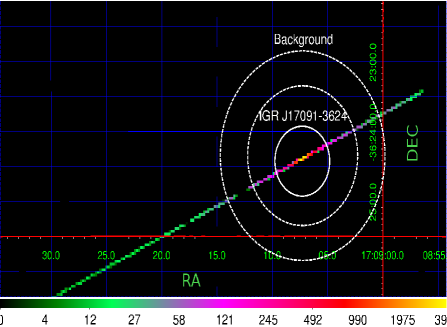
As per the XRT threads , if the Window-timing mode data has more than 100 counts/sec then pile-up may occur in the imaging. For the observations of this source the count rate is less than 30. Hence the image is completely devoid of pile-up effect. We choose a circle of radius 30$\arcsec$ for the source region and an annular region is taken far away from the source for the background, as shown in Figure 1. The x-axis is Right Ascension (RA) and y-axis is Declination (DEC). We have also provided a color-bar at the bottom of the figure indicating the intensity. We apply a scaling factor by editing the BACKSCAL keyword for both source and background regions (see Radhika et al. 2016b for details).

Uncertainty in position of the source has been taken care of, by applying the position dependent rmfs for the grade 0-2. The ARF files are obtained by making use of the exposure map with xrtmkarf. We re-bin the source spectral data to contain a minimum of 25 counts per bin with the ftool grppha.

Fig. 1 : Image of the source IGR J17091$-$3624 taken with SWIFT-XRT and displayed in logarithmic scale. The dotted annular region has inner radius 60$\arcsec$ and outer radius of 90$\arcsec$ while the circular source region has a radius of 30$\arcsec$. Both regions are centred at the RA and Dec of the source.

The extraction of XRT timing data is performed by following the procedure mentioned in the XRT analysis guide . We consider the event data of XRT and select the source and background regions. For the respective regions, we generate source and background light curves. A time bin resolution of 0.018 sec is chosen as multiple of the minimum XRT time resolution of 1.8 msec, while obtaining the light curves. With the help of lcmath, we subtract the background light curve from the source. Thus we obtain the background subtracted light curve, which is used for further analysis. Detailed procedures maybe referred to in Radhika et al. 2016b.

2.2 NuSTAR data reduction

The NuSTAR mission (Harrison et al., 2013) consists of two independent grazing incidence telescopes operating in the high energy X-rays (3 - 79 keV). It has two Focal Plane Modules (FPM) referred to as FPMA and FPMB. NuSTAR has six TOO observations of IGR J17091$-$3624 which are carried out over different phases of the outburst. Since four NuSTAR observations are quasi-simultaneous with SWIFT, we could obtain broad-band spectra for the energy range of 0.5 - 79 keV. We have got statistically sufficient counts for these broad-band spectra, in all the states of the source as illustrated in Table LABEL:tab:obs of appendix.

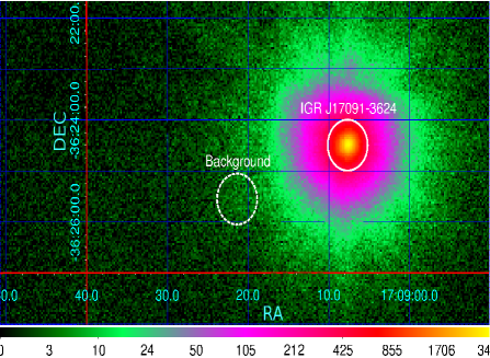
Data from both FPM detectors of the NuSTAR observatory is used for obtaining spectra between 3 - 79 keV. We follow the procedures mentioned in the NuSTAR guide and extract the level 2 data using the ftools command nupipeline. The source spectrum and light curve are extracted using a circular region of 30$\arcsec$ centred at the source RA and DEC with the $ds9$ tool. For background spectrum, we use another source free circular region of 30$\arcsec$ (see Figure 2) taken from the same detector on which the source is seen. The ftool command nuproducts is used to extract the spectrum, light curve, response and arf files. The spectrum so obtained is re-binned to contain a minimum of 30 counts per bin using $grppha$ in order to use $\chi^{2}$ statistics while fitting the data.

Fig. 2 : Image shows IGR J17091$-$3624 captured with NuSTAR displayed in logarithmic scale. The source region is a circle of radius 30$\arcsec$ centred at the RA and Dec of the source while the background is a dashed circle of 30$\arcsec$ radius chosen slightly away from the source as is suggested in the NuSTAR quickstart guide.

3 Methodologies for ‘spectro-temporal’ analysis and phenomenological modelling

Using the spectral package of XSpec v 12.9 (Arnaud, 1996), we do spectral analysis of both XRT and NuSTAR data. We consider the energy ranges of 0.5 - 10 keV (XRT) and 3 - 79 keV (NuSTAR) respectively for the entire observation, as the optimum energy range with statistically significant photon counts. In this section we summarize the methodologies used to analyze spectral and temporal data, from both XRT and NuSTAR.

3.1 Analysis and modelling of XRT observations

We perform the spectral modelling using the diskbb (Mitsuda et al., 1984; Makishima et al., 1986) and powerlaw models. These models take into account the low-energy thermal emission from the Keplerian accretion disc and the Comptonization of the disc photons by the corona respectively. The phabs model (Wilms et al., 2000) is used to consider the interstellar absorption. From the spectral fits to all the data sets, the hydrogen column density (n_H) is found to be of the order of 1.1$\times$10²² cm^-2. This value is similar to the estimates of Krimm et al. 2011; Capitanio et al. 2012.

With the cflux model, we obtain the unabsorbed X-ray flux from the source in the XRT energy band of 0.5 - 10 keV. The XRT hardness ratio is estimated by calculating the ratio of fluxes in 4 - 10 keV and 0.5 - 4 keV. It is used to plot the HID along-with the total flux in the energy range of 0.5 - 10 keV. Using the err command of XSpec, we find the error limits for the flux values and different spectral parameters at 90 percent confidence interval. Here, the parameter for which error limits are to be obtained varies within a specific already assigned limit. This continues until the value of fit statistic becomes greater than the fit statistic obtained in the preceding step by a specific amount (Arnaud, 1996).

The package XRONOS v 5.22 is used for generating temporal XRT data with time resolution of 0.018 sec and bin size of 8192. This corresponds to a frequency range of 0.007 - 27.8 Hz for the PDS. Using powspec v 1.0, we generate PDS for the background subtracted light-curves so as to search for the presence of very low frequency QPOs. The PDS are normalized so that the integral gives the squared fractional rms variability. We also subtract the Poisson noise which is found to be a flat spectra with a power value of $\sim$2. Thus the resulting PDS is expressed as rms power (in units of rms²/Hz) variation with frequency.

The fractional rms variability is estimated for the frequency range of 0.007 - 1 Hz, since the noise is dominant above 1 Hz for most of the observations. As an example let us consider the initial observation of the source on day 0. The rms variability obtained for the frequency range of 0.007 - 1 Hz gives a value 39.3%. For 0.007 - 2 Hz the variability increases to 48%, while for 0.007 - 10 Hz it is $>$ 100%. Thus we find that above 1 Hz the rms variability is significantly dominated by band-limited noise. The rms value is calculated using the rectangle rule integration method, following the procedure given in RXTE cookbook .

As the count rates are low ($<$ 30 counts/sec), we divide the entire light curves into intervals of 2048 bins to obtain individual power spectrum. Then we co-add all these power spectra and average them to get statistically significant detection of QPOs. The different components of the PDS are fitted with multiple Lorentzians or else with a constant factor for noise dominated frequency range. The centroid of this Lorentzian ($\nu$) gives QPO frequency. Coherence of a QPO is defined by the Q-factor which is the ratio of centroid frequency ($\nu$) to width ($\lambda$). The QPO significance is calculated as the ratio of Lorentzian normalization to its negative error. QPO amplitude refers to the integrated rms power in the Lorentzian which is estimated using the rectangle rule integration method as mentioned earlier. For detailed procedure see Belloni & Hasinger 1990; Casella et al. 2004; McClintock & Remillard 2006.

3.2 Analysis and modelling of NuSTAR observations

The source IGR J17091$-$3624 during its 2016 outburst has been observed by NuSTAR on MJDs 57454, 57459, 57461, 57476, 57508 and 57534. We analyze all the six NuSTAR observations using both FPMA and FPMB detectors. The spectral fit parameters for data with both detectors is found to be similar. Hence, we present in this paper the analysis based on FPMA data only. It has to be also noted that the entire NuSTAR analysis has been done without inclusion of the fluorescent Fe line emission.

Four among the six TOO observations aid in the broad-band study of state evolution of the source. The broad-band spectrum in the energy range of 0.5 - 79 keV from SWIFT-XRT and NuSTAR is well fitted by the phenomenological models consisting of diskbb, ireflect and cutoffpl. The NuSTAR has excellent timing capability with a temporal resolution of 0.1 ms (Harrison et al., 2013). Since we intend to search for the presence of low frequency QPOs, background subtracted light curves of resolution 0.5 sec are generated. The light curves are then divided into 8192 intervals, to result in a frequency range of 0.0002 - 1 Hz in the PDS. Here, also we model the different components of the PDS and hence study the properties of QPOs. Background subtracted light curves of same bin time are also generated for different energy bands (3 - 15 keV, 15 - 79 keV and 3 - 79 keV). Light curves are used to produce PDS for various energy bands and fitted with Lorentzians to extract different features, as mentioned above.

All these procedures discussed for analysis of the data are based on phenomenological models. In the following section, we will discuss in detail the results from our temporal and spectral modelling of the XRT and NuSTAR observational data for the entire outburst.

4 Results

We present here the results of detailed spectral and temporal analysis of the source IGR J17091$-$3624 during its 2016 outburst. In subsection 4.1 we give the details of results obtained using phenomenological fits to the X-ray spectra, and from temporal analysis. The evolution of the different HID regions are discussed here. We also give a description of evidence obtained for coherent variabilities and evolution of QPOs during some of the HID regions in 4.2. Further, we give an account of the spectral modelling performed with two component model and the variations of relevant parameters.

4.1 Evolution of spectral and temporal features in the outburst profile

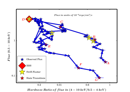
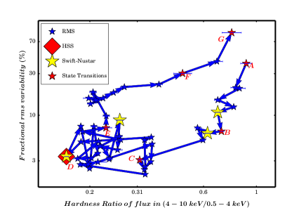
In Figure 3, we present the evolution of observed flux. The unabsorbed value of flux in 0.5 - 10 keV, along-with the contribution of disc and powerlaw fluxes are shown in panels a, d and e respectively. The variation of spectral parameters i.e. photon index $\Gamma$ and disc temperature T_in are represented in panels b and c. The evolution of BAT count rate obtained from BAT light curve of the source is shown in panel f. The XRT hardness ratio and fractional rms variability obtained from power spectra for all observations are represented in panels g and h respectively. The evolution of total flux as a function of hardness ratio for XRT observations is shown in the hardness intensity diagram (HID) in left panel of Figure 4. On the right panel of Figure 4 we show the variation of the fractional rms variability w.r.t. the hardness ratio in a hardness rms diagram (HRD). Phenomenological fitting performed for broad-band spectra of quasi-simultaneous XRT and NuSTAR observations are also discussed in this section and shown in Figure 8.

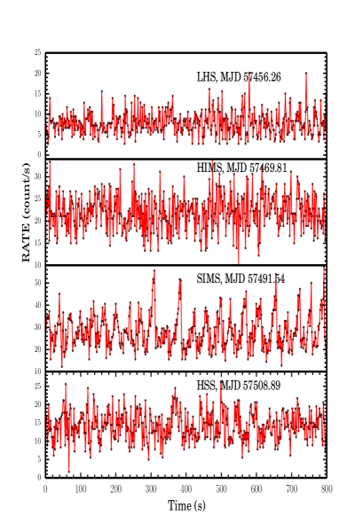
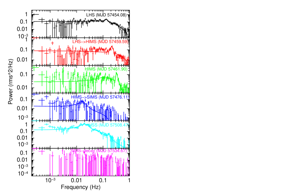
In this section we also present the results on unique temporal properties of the source. In Figure 5, we show the variation of XRT light-curves and power spectra for various phases of the outburst. The NuSTAR power spectra are presented in Figure 6. Different types of variabilities that are observed in XRT light-curves are shown in Figure 7.

Below, we summarize the evolution of spectral and temporal parameters during the different regions of the HID and HRD (marked from A to G in Figure 4) as the outburst progresses. As mentioned in section 1, we refer to the general understanding of spectral state classification (Belloni et al., 2005; McClintock & Remillard, 2006; Nandi et al., 2012) while studying the HID. In Table 1 we have given the values of different spectral and temporal parameters obtained from XRT observations, while Table 2 presents the results from temporal analysis of specific XRT and NuSTAR observations. Tables 3 and 4 show results from spectral analysis of broad-band observations from the different HID regions. We bring into notice once again that MJD 57445 is considered as day 0 throughout the entire manuscript.

All regions discussed in the following sections correspond to regions of Figure 4.

Table 1 : Variation of spectral and temporal parameters obtained from XRT observations. It has to be noted that the X-ray flux values are quoted here in units of $10^{-9}$ erg cm^-2 sec^-1, and the fractional rms variability has been estimated in the frequency range of 0.007 - 1 Hz

. Spectral state MJD 0.5 - 10 keV flux Hardness Ratio Photon index, $\Gamma$ T_in rms(%) LHS-rise 57445.35 2.524${}^{+0.09}_{-0.09}$ 0.906${}^{+0.049}_{-0.049}$ 1.411${}^{+0.076}_{-0.096}$ - 39.314 57447.27 3.105${}^{+0.104}_{-0.103}$ 0.818${}^{+0.038}_{-0.038}$ 1.463${}^{+0.068}_{-0.068}$ - 20.793 57450.94 5.122${}^{+0.206}_{-0.206}$ 0.849${}^{+0.048}_{-0.048}$ 1.462${}^{+0.083}_{-0.083}$ - 20.343 57452.53 6.306${}^{+0.153}_{-0.153}$ 0.688${}^{+0.023}_{-0.023}$ 1.587${}^{+0.050}_{-0.050}$ - 14.985 57456.26 7.755${}^{+0.113}_{-0.113}$ 0.803${}^{+0.016}_{-0.016}$ 1.479${}^{+0.030}_{-0.030}$ - 12.475 HIMS-rise 57459.57 9.940${}^{+0.167}_{-0.166}$ 0.688${}^{+0.015}_{-0.015}$ 1.727${}^{+0.037}_{-0.036}$ - 10.828 57460.71 1.028${}^{+0.018}_{-0.018}$ 0.713${}^{+0.018}_{-0.018}$ 1.566${}^{+0.037}_{-0.038}$ - 6.553 57461.90 1.214${}^{+0.019}_{-0.019}$ 0.623${}^{+0.015}_{-0.015}$ 1.745${}^{+0.036}_{-0.036}$ - 6.218 57467.88 1.276${}^{+0.020}_{-0.019}$ 0.566${}^{+0.014}_{-0.022}$ 1.727${}^{+0.032}_{-0.032}$ - 7.168 57468.02 1.355${}^{+0.021}_{-0.021}$ 0.596${}^{+0.012}_{-0.013}$ 1.706${}^{+0.032}_{-0.032}$ - 5.201 57469.81 2.245${}^{+0.026}_{-0.026}$ 0.323${}^{+0.003}_{-0.012}$ 1.813${}^{+0.151}_{-0.131}$ 0.596${}^{+0.049}_{-0.056}$ 3.081 57470.81 2.595${}^{+0.031}_{-0.030}$ 0.338${}^{+0.005}_{-0.005}$ 2.044${}^{+0.016}_{-0.018}$ 1.104${}^{+0.056}_{-0.056}$ 2.387 57474.60 2.357${}^{+0.032}_{-0.032}$ 0.341${}^{+0.006}_{-0.006}$ 2.039${}^{+0.022}_{-0.023}$ 1.119${}^{+0.051}_{-0.051}$ 2.104 57479.84 2.054${}^{+0.023}_{-0.0234}$ 0.182${}^{+0.002}_{-0.002}$ 1.978${}^{+0.023}_{-0.024}$ 1.092${}^{+0.032}_{-0.031}$ 2.724 SIMS-rise 57482.69 2.054${}^{+0.024}_{-0.024}$ 0.196${}^{+0.003}_{-0.003}$ 2.009${}^{+0.022}_{-0.023}$ 1.064${}^{+0.036}_{-0.035}$ 2.741 57490.74 1.923${}^{+0.109}_{-0.109}$ 0.216${}^{+0.017}_{-0.017}$ - 1.269${}^{+0.115}_{-0.137}$ 2.91 57491.54 2.061${}^{+0.024}_{-0.023}$ 0.365${}^{+0.005}_{-0.005}$ - 1.239${}^{+0.019}_{-0.019}$ 4.678 57492.95 2.056${}^{+0.023}_{-0.023}$ 0.360${}^{+0.005}_{-0.005}$ - 1.332${}^{+0.021}_{-0.022}$ 2.929 57501.64 1.967${}^{+0.021}_{-0.021}$ 0.341${}^{+0.005}_{-0.005}$ - 1.369${}^{+0.021}_{-0.021}$ 2.576 57502.38 2.118${}^{+0.023}_{-0.023}$ 0.339${}^{+0.005}_{-0.005}$ - 1.285${}^{+0.026}_{-0.027}$ 5.207 57505.77 2.270${}^{+0.025}_{-0.025}$ 0.362${}^{+0.006}_{-0.006}$ 1.676${}^{+0.324}_{-0.210}$ 1.082${}^{+0.057}_{-0.078}$ 5.596 57506.58 2.137${}^{+0.023}_{-0.023}$ 0.183${}^{+0.004}_{-0.004}$ 1.869${}^{+0.099}_{-0.084}$ 1.254${}^{+0.025}_{-0.026}$ 4.952 HSS-rise 57508.89 1.759${}^{+0.021}_{-0.021}$ 0.159${}^{+0.003}_{-0.003}$ - 1.314${}^{+0.030}_{-0.031}$ 3.363 SIMS-decay 57512.02 1.701${}^{+0.019}_{-0.019}$ - 1.333${}^{+0.029}_{-0.031}$ 4.704 57513.47 1.808${}^{+0.023}_{-0.023}$ 0.183${}^{+0.003}_{-0.003}$ - 1.312${}^{+0.023}_{-0.024}$ 7.485 57516.81 1.362${}^{+0.019}_{-0.019}$ 0.199${}^{+0.004}_{-0.004}$ - 1.090${}^{+0.020}_{-0.021}$ 2.454 57519.79 2.220${}^{+0.044}_{-0.044}$ 0.207${}^{+0.005}_{-0.005}$ - 1.087${}^{+0.032}_{-0.034}$ 7.437 57521.31 2.193${}^{+0.036}_{-0.036}$ 0.216${}^{+0.005}_{-0.005}$ 2.628${}^{+0.263}_{-0.530}$ 1.299${}^{+0.252}_{-0.149}$ 3.663 57524.50 1.502${}^{+0.022}_{-0.022}$ 0.202${}^{+0.004}_{-0.004}$ 1.791${}^{+0.254}_{-0.186}$ 0.855${}^{+0.059}_{-0.091}$ 3.229 57524.77 5.216${}^{+0.125}_{-0.125}$ 0.177${}^{+0.007}_{-0.007}$ - 1.082${}^{+0.044}_{-0.047}$ 3.18 57527.56 1.521${}^{+0.021}_{-0.021}$ 0.217${}^{+0.004}_{-0.004}$ 2.163${}^{+0.020}_{-0.021}$ 1.057${}^{+0.062}_{-0.063}$ 5.027 57532.88 1.477${}^{+0.022}_{-0.022}$ 0.242${}^{+0.005}_{-0.005}$ 2.125${}^{+0.159}_{-0.126}$ 0.730${}^{+0.106}_{-0.238}$ 3.241 57533.03 1.407${}^{+0.031}_{-0.031}$ 0.241${}^{+0.007}_{-0.007}$ 2.244${}^{+0.197}_{-0.231}$ 0.889${}^{+0.259}_{-0.604}$ 3.139 57534.67 1.164${}^{+0.017}_{-0.017}$ 0.267${}^{+0.008}_{-0.008}$ 2.279${}^{+0.059}_{-0.061}$ - 8.80 57538.35 1.330${}^{+0.043}_{-0.043}$ 0.261${}^{+0.012}_{-0.012}$ 2.092${}^{+0.064}_{-0.065}$ - 4.012 57539.07 1.127${}^{+0.021}_{-0.021}$ 0.221${}^{+0.005}_{-0.005}$ 2.109${}^{+0.212}_{-0.175}$ 0.854${}^{+0.129}_{-0.239}$ 4.417 57540.07 9.424${}^{+0.190}_{-0.190}$ 0.266${}^{+0.007}_{-0.007}$ 2.188${}^{+0.041}_{-0.041}$ - 5.714 57543.06 1.240${}^{+0.020}_{-0.020}$ 0.269${}^{+0.006}_{-0.006}$ 2.218${}^{+0.035}_{-0.035}$ - 5.241 HIMS-decay 57561.00 8.523${}^{+0.166}_{-0.166}$ 0.186${}^{+0.005}_{-0.005}$ 2.545${}^{+0.045}_{-0.046}$ - 6.510 57569.71 7.321${}^{+0.279}_{-0.279}$ 0.233${}^{+0.013}_{-0.013}$ 2.399${}^{+0.081}_{-0.082}$ - 7.187 57571.83 7.768${}^{+0.163}_{-0.163}$ 0.234${}^{+0.007}_{-0.007}$ 2.397${}^{+0.045}_{-0.045}$ - 9.799 57573.48 7.151${}^{+0.168}_{-0.167}$ 0.206${}^{+0.007}_{-0.007}$ 2.446${}^{+0.049}_{-0.049}$ - 18.421 57575.68 7.442${}^{+0.166}_{-0.166}$ 0.211${}^{+0.006}_{-0.006}$ 2.456${}^{+0.050}_{-0.051}$ - 14.922 57580.73 6.644${}^{+0.226}_{-0.227}$ 0.197${}^{+0.010}_{-0.010}$ 2.507${}^{+0.079}_{-0.081}$ - 15.684 57581.01 5.962${}^{+0.130}_{-0.130}$ 0.227${}^{+0.007}_{-0.007}$ 2.424${}^{+0.050}_{-0.051}$ - 15.671 57583.53 5.934${}^{+0.124}_{-0.124}$ 0.201${}^{+0.006}_{-0.006}$ 2.524${}^{+0.051}_{-0.052}$ - 13.525 57591.64 4.667${}^{+0.103}_{-0.103}$ 0.251${}^{+0.008}_{-0.008}$ 2.348${}^{+0.055}_{-0.055}$ - 18.177 57593.95 4.381${}^{+0.137}_{-0.137}$ 0.279${}^{+0.011}_{-0.011}$ 2.295${}^{+0.072}_{-0.073}$ - 21.079 57595.48 3.752${}^{+0.089}_{-0.089}$ 0.389${}^{+0.013}_{-0.013}$ 2.095${}^{+0.055}_{-0.055}$ - 22.603 LHS-decay 57612.03 1.413${}^{+0.061}_{-0.061}$ 0.682${}^{+0.038}_{-0.038}$ 1.723${}^{+0.098}_{-0.098}$ - 41.43 57617.82 5.183${}^{+0.313}_{-0.313}$ 0.787${}^{+0.073}_{-0.073}$ 1.587${}^{+0.143}_{-0.143}$ - 88.65

Fig. 3 : Evolution of total X-ray flux in 0.5 - 10 keV, spectral parameters of photon index and disk temperature, contribution of disc flux and powerlaw flux in 0.5 - 10 keV, BAT count rate in 15 - 50 keV, hardness ratio and fractional rms variability in % computed in 0.007 - 1 Hz frequency range are presented in different panels. All the flux values are given in units of $10^{-9}$ erg cm^-2 sec^-1. The grids (vertical lines) are used to differentiate between the different spectral states. See text for details.

Fig. 4 : Left panel : Hardness-Intensity diagram (HID) showing evolution of the hardness ratio (flux in 4 - 10 keV / 0.5 - 4 keV) with total unabsorbed flux in 0.5 - 10 keV given in units of $10^{-9}$ erg cm^-2 sec^-1 is shown. Right panel : Hardness-rms diagram (HRD) depicting evolution of hardness ratio w.r.t fractional rms variability (in %) estimated in a frequency range of 0.007 - 1 Hz. The different regions in the HID & HRD from A to G denote the spectral states of hard, hard intermediate, soft intermediate and soft state during the rising and decaying phase of the outburst respectively. The four quasi-simultaneous broad-band observations with XRT+NuSTAR are marked in yellow stars.

4.1.1 Region AB

Observations during days 0.35 to 13.8 are considered part of the region AB. These observations belong to the rising phase of the outburst.

The XRT spectra are well modelled with phabs*(powerlaw) and do not require the diskbb. As an example from the spectral fits on day 13.8, we obtain $\chi^{2}/dof$ as 360.01/340. An inclusion of diskbb results in $\chi^{2}/dof$ of 358.99/338 but with incorrect values for the different diskbb parameters. An ftest to this observation provides F-statistic of 0.48 and probability of 0.62. These prove that the disc component is not necessary for the fits.

During these initial days, we observe the XRT flux and spectral photon index to increase as shown in Figure 3 and Table 1. It is also evident that the XRT hardness ratio decreases from 0.906$\pm{0.049}$ to 0.803$\pm{0.016}$ (see Table 1, Figure 4 and panel g of Figure 3). The BAT count rate in 15 - 50 keV corresponding to the hard flux contribution is also observed to increase from 0.007 to 0.017 (panel f of Figure 3). The temporal analysis suggest that the fractional rms variability decreases from 39 to 10 percent (bottom panel of Figure 3, right panel of Figure 4, Table 1). Based on these variations of spectral and temporal parameters, we understand that this region corresponds to the low hard state in the rising phase of the outburst.

We find that the value of photon index is similar to that obtained during the 2011 outburst of the source by Capitanio et al. 2012. Yet, the hardness ratio is more than that in 2011 and is similar to that observed for typical BH transients during their LHS (Belloni et al., 2005; McClintock & Remillard, 2006; Nandi et al., 2012).

4.1.2 Region BC

This region consists of observations from days 14.58 to 34.8. During the observations for days 14.58 to 23.0, we find that the XRT spectral fits can be performed using the model phabs*(powerlaw). The $\chi^{2}/dof$ on day 22.8 is found to be of 407.84/353. When a disc component is included to this fit the $\chi^{2}/dof$ is obtained as 407.59/351. An F-test to these spectral fits gives the F-statistic value as 0.107 and a probability of 0.89 which is statistically very high. The fit results also show the disc temperature value to be 0.794+/-1.44 and disc normalization is 1.330+/-5.85 (the errors are quoted in 1-$\sigma$) which are statistically incorrect. Thus it is clear that the disc component is not required for these observations.

An estimate of the hardness ratio shows that it reduces from 0.8 during the LHS to 0.59 during these initial observations. Also, the fractional rms variability decreases from 14% during LHS to $\approx$ 8%. Thus we understand that the source has transited from the LHS.

The diskbb model is found to be necessary to the fits from day 24.8 on-wards. The spectral fit to the XRT data on day 34.8 improves the $\chi^{2}/dof$ from 862.99/433 to 465.05/431, when a disc component is included along-with the powerlaw. F-test results give F-statistic probability of $1.37\times 10^{-58}$ implying statistical significance of the disc component.

During the observations in region BC, the photon index is observed to increase to 2.0${}^{+0.03}_{-0.02}$ as shown in Table 1. The disc temperature $T_{in}$ changes randomly between 0.59$\pm{0.05}$ keV and 1.1$\pm{0.05}$ keV (Figure 3). The total flux is observed to increase with the maximum being observed on day 25.8 (Figure 3). The disc flux is observed to be increasing whereas the powerlaw flux decreases (panels d and e of Figure 3).

Also from panel g of Figure 3 we find that the BAT count rate decreases to an average of 0.006. With respect to the LHS, the hardness ratio is observed to decrease (see region BC in Figure 4). The temporal properties show that the fractional rms variability decreases from 7 to 2 percent (panel h of Figure 3, right panel of Figure 4). All these characteristics point out that the contribution of hard flux decreases while that of disc flux is increasing. Hence we understand that the source is in the HIMS for these observations. Variations in the high energy spectra occurring during this HIMS are discussed below in section 4.2.

4.1.3 Region CD

The observations during days 45.74 to 61.57 have been considered in the region CD in Figure 4. Their energy spectra can be well fitted with the model phabs*(diskbb). The powerlaw component is not at all required for the fits. As an example on day 56.64 the spectral fit results in a $\chi^{2}/dof$ of 539/446 when we model it using a disc component. But inclusion of a powerlaw component results in incorrect value of the parameters.

During the observations in region CD of the HID, the disc temperature do not vary significantly (Figure 3, Table 1). Although the hardness ratio is decreasing, it changes randomly between 0.365 to 0.183 (see Figure 4). This range of hardness ratio value matches well with that observed by Capitanio et al. 2012 during the intermediate state of 2011 outburst.

As evident in Table 1 the total flux also varies randomly and the BAT count rate decreases to 0.004 (panels a and f of Figure 3 respectively). We note that there is a significant reduction in the fractional rms variability to 4% along-with the hardness ratio as evident in the HRD (right panel of Figure 4). The fact that the spectra softens in comparison to HIMS and both hardness ratio and rms value decreases, is strongly indicative of the source being in the SIMS during these observations.

4.1.4 Point D

On day 63.89 (i.e. MJD 57508.89), we observe that the XRT spectrum showed the presence of only a disc component. The fit using model phabs*(diskbb) results in a $\chi^{2}/dof$ of 426.16/395. When we include a powerlaw the reduced $\chi^{2}$/dof is found to be of 418.45/393. An ftest to these values show a F-statistic of 3.62. Since the value is higher it is evident that the spectra consists of only the disc component.

The value of hardness ratio estimated after the spectral fit shows that it has decreased from those in the other regions and reached to a minimum of 0.159. The flux value continues to be closer to the maximum value of $\sim 2\times 10^{-9}$ erg cm^-2 sec^-1 (see the asterisk marked in a red diamond at point D in both left and right panels of Figure 4; also Table 1). The disc temperature is at its maximum of $1.31\pm 0.03$ keV. The fractional rms variability is around 3 percent. These variations of the spectral and temporal parameters as shown in Table 1 indicate further softening of the spectra w.r.t region CD.

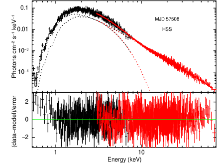
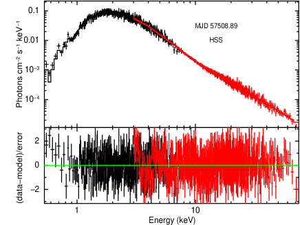
In order to have stronger evidence on this softening, we performed the broad-band spectral fit of the energy spectrum (see section 4.2 below for details) corresponding to this observation using SWIFT-XRT and NuSTAR as shown in the Figure 8 (right panel). In this case it is very clear that the high energy spectrum is having less counts above 60 keV than observed for HIMS in left panel of Figure 8. It is found that the flux contribution from disc is significant (33 percent) in the broad-band spectra (which is more than the contribution of 19 percent during the decay phase - see below). The powerlaw photon index from the broad-band fit is of 2.4 which also indicates a relatively softer state. Also, these variations of spectral and temporal properties of the source are similar to those observed for many other black hole binaries like GX 339$-$4, H 1743$-$322 during their HSS (Homan et al., 2001; Belloni et al., 2005; McClintock & Remillard, 2006; Nandi et al., 2012). Hence, we presume that the source probably has reached HSS around day 63.89.

4.1.5 Region DE

After the short duration in HSS, we notice from panel a of Figure 3 and Figure 4 that the source enters its declining phase around day 67.02. The observations for the period of 67.02 to 116.0 is represented in region DE.

With respect to point D, we find that on day 67.02 the total flux decreases to $1.7\times 10^{-9}$ erg cm^-2 sec^-1, while the hardness ratio is in the range of 0.183 - 0.269 (region DE in Figure 4). The spectra are fitted with both disc and powerlaw flux models ($\chi^{2}/dof$ of 324.86/339 on day 79.50). For a few of the observations until day 114.80 the spectral fits require only powerlaw ($\chi^{2}/dof$ of 253.77/245 on day 114.80).

The photon index is observed to vary around 2.2, and disc temperature is observed to now decrease from its previous value during the HSS (Figure 3, Table 1). The broad-band observation on day 89 (MJD 57534) also give similar value for the photon index and disc temperature. The disc emission contributes 19 percent to the total flux which is lesser than that found for the broad-band observation in the HSS. The temporal studies show that the light curve exhibits variabilities only on day 67.02 (see last panel of Figure 7), and not for rest of the observations. The fractional rms variability is found to be around 6 - 11 percent (panel h of Figure 3, right panel of Figure 4) and the PDS have only broad-band noise. These indicate that the source has entered SIMS during these observations in the beginning of the decay phase.

4.1.6 Region EF

This region corresponds to days 124.9 to 150. For these observations, the spectra are well-fitted with the powerlaw model. For the observation on day 114.80 during the decay phase of the source, when the spectra is fitted with phabs(powerlaw) it results in a $\chi^{2}$/dof of 253.77/245. Inclusion of a disc component results in a $\chi^{2}$/dof of 253.27/243. An F-test to this results in F-statistic value of 0.239 with probability of 0.787. These high values rule out the possibility of presence of a disc component.

Although there is no disc component and the spectral photon index is observed to be having an average of 2.2 (Figure 3), we find that the hardness ratio has increased w.r.t its value during region DE in Figure 4. Also, the total flux decreases to $0.7\times 10^{-9}$ erg cm^-2 sec^-1. The fractional rms variability varies between a minimum of 13% and a maximum of $\sim$22%, with the PDS exhibiting only broad-band noise. The light curve does not exhibit any oscillatory features. The increase in hardness ratio, powerlaw flux contribution and the rms w.r.t the region DE suggest that the source is in HIMS of decay phase for the observations of region EF. We do not consider these as part of a LHS since the values of photon index, hardness ratio and rms variability are lesser in comparison to the following observations discussed below.

4.1.7 Region FG

Following the HIMS during days 167 and 172 the spectral fit requires only a powerlaw component. We observe that the photon index of the spectra decreases to $<$ 1.7 and the hardness ratio increases to $\sim$0.787${\pm 0.073}$ (see Table 1). Here, we find that the light curves do not display any oscillations, and the PDS have only broad-band noise. Since for these observations, the XRT image displays double streaks, we have excluded the events corresponding to the shortest time interval and hence removed the second streak. We then find that the fractional rms values for these days become 41.43% and 88.65% respectively, as shown in the panel h of Figure 3. There are no good observations after this day due to incorrect imaging in the window-timing mode of XRT and also lesser counts. So, the observed increase in hardness ratio, fractional rms variability and the decline in photon index suggests that the source exists in the hard state of decay phase as shown in region FG in Figure 4.

Thus based on the phenomenological spectral modelling, we understand that the source exhibits spectral state transitions, which results in a complete ‘q’-profile for the 2016 outburst. In the following sub-section, we present the details of temporal variabilities and QPOs observed during the different HID regions.

4.2 Presence of coherent variabilities and evolution of QPOs

For the observations of the source in LHS and HIMS (regions AB and BC), we did not find any signature of oscillations/variabilities (left panel of Figure 5). As the source enters the SIMS (region CD), we observe that the light curves exhibit variabilities/oscillations. This characteristic is similar to that observed for this source during its previous outburst in 2011. We find that for 9 continuous observations i.e. from days 46.54 to 61.58, these oscillations are present (left panel of Figure 5 and Figure 7). The light curves have a period of minimum 50 sec on days 49.60, 52.80, 55.26 and a maximum of 450 sec on day 55.26, implying the frequency range of tens of mHz. The intensity of the different peaks in the light curves varies randomly in the range of 40 to 60 counts/sec. These observations exist in the top left portion of the HID (Figure 4) with a clear random variation of both hardness ratio and total flux. This variation of source flux in the light curve is similar to that observed during the heartbeat phase of the 2011 outburst where almost 9 types of variabilities were observed. The source was found to remain trapped in this phase throughout the 2011 outburst (Capitanio et al., 2012; Court et al., 2017). On a comparison with GRS 1915$+$105, the oscillations/variabilities we find for the 2016 outburst can be categorized as similar to the $\rho$-class (see Belloni et al. 2001 for details on different variability classes).

The temporal analysis for the observation of point D (i.e. a possible HSS) shows that the light curve exhibits variabilities/oscillations (see 4th panel on left side of Figure 5). These oscillations are found to be weaker (maximum intensity of 20 counts/sec) in comparison to those observed during SIMS. An energy dependent study of the NuSTAR light curve shows that the variability is prominent at lower energies.

During the rising phase LHS and HIMS i.e. regions AB and BC respectively, we are able to detect weak QPOs. The XRT PDS show QPOs of frequency increasing from 0.15 Hz to 0.18 Hz (see Table 2 and right panel of Figure 5) during the LHS. A very prominent QPO of 0.13$\pm{0.03}$ Hz with rms amplitude of 6.20 percent is seen in the NuSTAR PDS during day 9 (top panel of Figure 6; see also Xu et al. 2017). Previous outburst of this source has shown presence of constant frequency QPOs during its LHS (Iyer & Nandi, 2013; Iyer et al., 2015).

Fig. 5 : The XRT light curve and power density spectrum corresponding to the four states (LHS, HIMS, SIMS and HSS) of the source IGR J17091$-$3624 during the rising phase of its 2016 outburst are shown in two panels. The light curves do not show any signature of variability during LHS and HIMS. During the SIMS & HSS variabilities of time period 50 to 450 sec are observed. Weak detection of QPOs at 0.15 Hz and 2.15 Hz is seen in LHS and HIMS respectively (see Figure 6 for strong detection of QPOs during the same period). Corresponding to the observations where variability is observed, QPOs are detected around 20 mHz to 30 mHz during the SIMS and HSS.

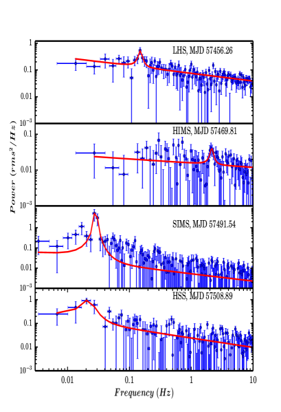
The QPO frequency increases up to a maximum of 2.15 Hz during the HIMS. The quasi-simultaneous NuSTAR observations during this period also indicate strong signatures of QPOs of frequencies $0.217\pm 0.002$ Hz on day 14.59 (see Xu et al. 2017) and $0.326\pm 0.005$ on day 16.90 respectively (see the 2nd and 3rd panels of Figure 6). This is similar to the 2011 outburst where also a gradual increase of QPO frequencies was observed (Iyer & Nandi, 2013; Iyer et al., 2015).

Based on the frequency range, their rms and Q-factor, these QPOs observed during hard and hard-intermediate states can be considered of type C. These QPOs are found to evolve with time i.e. the QPO frequency increases as the source moves from hard to hard-intermediate state. In our recent paper Sreehari et al. 2018 we we have studied this evolution and discussed the physical significance of the same.

We find that just a few days before the transition to the next state i.e. on day 31.11 (MJD 57476.11) the NuSTAR light curve shows weak signature of variabilities. The resultant PDS gives a weak 16.4$\pm$2 mHz QPO (see 4th panel of Figure 6 and Table 2).

A detailed study of the PDS for the 2016 outburst show that for all the observations during the SIMS, the power spectrum has a powerlaw nature. These power spectra give strong indication of the presence of very low frequency QPOs (see right panel of Figure 5) in the range of 20 to 30 mHz. It has to be noted that a few of the QPOs have lesser values of Q-factor and amplitude unlike the typical values found in other BH sources (Casella et al., 2004). The values of different parameters of these QPOs are given in Table 2.

During the observation corresponding to point D of HID, both the XRT and NuSTAR PDS indicate presence of a low frequency broad QPO like feature at 21.4 mHz and 20.7 mHz respectively. The latter has a strong significance 5.32 and rms amplitude of 5.71 percent (see Table 2 and 5th panel of Figure 6). In the NuSTAR PDS there is also a weak peaked component around 0.16 Hz which has a Q-factor of 5, rms amplitude of 1.58 but significance of 2.3 only. An energy dependent study of the NuSTAR observation shows that the broad mHz QPO and weak feature are observed only at lower energies (3 - 25 keV).

Table 2 : Values of QPO frequencies observed during the rising phase of LHS, HIMS, SIMS and ‘possible’ HSS for IGR J17091$-$3624. mHz QPOS are observed during the days when the light curve exhibits oscillations. Strong presence of QPOs is indicated by the NuSTAR observations during the different spectral states. Here, MJD 57445 has been considered as day 0.

MJD	Day	Instrument	QPO frequency	Q-factor	Significance	amplitude
			(Hz)			(rms %)
LHS
57454.08	9.08	NuSTAR	0.133$\pm{0.03}$	6.04	4.52	6.20
57456.26	11.26	XRT	0.151$\pm{0.01}$	6.55	1.68	4.36
HIMS
57459.58	14.58	XRT	0.189$\pm{0.01}$	4.25	1.32	3.79
57459.59	14.59	NuSTAR	0.217$\pm 0.002$	7.35	6.45	1.88
57461.80	16.80	XRT	0.332$\pm 0.005$	7.81	1.30	2.77
57461.90	16.90	NuSTAR	0.326$\pm 0.005$	5.82	5.75	1.89
57469.81	24.81	XRT	2.149$\pm 0.1$	7.16	1.8	2.58
HIMS$\rightarrow$SIMS
57476.11	31.11	NuSTAR	16.4${\pm 2}$ mHz	1.31	3.92	0.61
SIMS
57491.54	46.54	XRT	28${}^{+1}_{-2}$ mHz	3.91	3.81	3.71
57494.61	49.61	XRT	25${\pm 2}$ mHz	1.15	4.81	4.30
57497.80	52.80	XRT	36${}^{+2.4}_{-3.2}$ mHz	4.17	4.22	8.92
57500.26	55.26	XRT	28${\pm 3}$ mHz	2.07	2.95	4.81
57502.38	57.38	XRT	28${\pm 2}$ mHz	3.57	3.35	3.87
57505.77	60.77	XRT	30${\pm 1.5}$ mHz	1.76	6.50	5.90
57506.58	61.58	XRT	19.7${}^{+4}_{-3}$ mHz	1.32	2.52	3.71
HSS
57508.47	63.47	NuSTAR	20.7${\pm 0.06}$ mHz	0.92	5.32	5.71
57508.89	63.89	XRT	21.4${\pm 0.001}$ mHz	1.69	3.50	3.56

Fig. 6 : Power density spectra during the 6 TOO NuSTAR observations. The fits to these spectra show clear indication of strong QPOs during LHS, HIMS, transition to SIMS-rise and the possible HSS, while broad-band noise is seen for decay phase of SIMS.

Fig. 7 : Variability/oscillations found during the continuous observations in rising phase of SIMS (MJD 57445 corresponds to day 0). The time period varies randomly from 50 to 450 sec for these light curves.

In the next subsection we explain the results obtained by modelling the broad-band spectra (XRT + NuSTAR) using the phenomenological models.

4.3 Phenomenological modelling of the broadband spectra

As mentioned earlier for the 2016 outburst of IGR J17091-3624 there are six NuSTAR observations of which four are quasi-simultaneous observations with SWIFT-XRT. We fit all these broadband spectra with different models to search for the presence of various features like high energy cut-off, reflection and presence of disc.

It has to be noted that although the NuSTAR exposure time is longer, the duration of XRT observation falls within the NuSTAR exposure period. These are not strictly simultaneous, but can be called quasi-simultaneous. The black hole accretion systems are generally dynamic and significant spectral changes may occur over the duration. Any considerable change in the spectrum in this period would have been evident from the energy spectrum obtained from the two instruments. But we observe that there is good overlap between the spectra from two instruments with no evident offset. We also note that the combined spectral fit of the quasi-simultaneous observations results in $\chi^{2}$/dof value around unity.

We initially modelled all these observations with compTT and the $\chi^{2}$/dof for these cases are provided in the appendix in Table 6. Although the $\chi^{2}$/dof values look reasonable statistically, there are lots of internal inconsistencies in the model parameters. For example on day 63 (MJD 57508), the model diskbb+compTT fits the data well but the disc temperature Tin = 1.097 keV is not consistent with soft photon temperature T₀ = 0.08 keV of compTT. In fact extra disc component should not have been required along with compTT, but for a good statistical fit diskbb is required. Hence we do not present here the parameter studies based on compTT model.

So we took the broadband spectra corresponding to HIMS and fitted it with a powerlaw component. This resulted in a $\chi^{2}/dof~{}=~{}1475.41/1116$. The fit improved when we used a cutoffpl instead of the powerlaw giving a $\chi^{2}/dof~{}=~{}1290.67/1115$. This fit had some large residual values around 30 keV. We added a component ireflect to take care of the reflection contribution from ionized material and this reduced the $\chi^{2}/dof$ to $1202.27/1113$. So we could obtain a decent $\chi^{2}$/dof value with the model phabs(ireflect*cutoffpl) for the case of hard and hard-intermediate states. But for fitting the spectra of the softer states the inclusion of the diskbb component is required. Thus we use the most general phenomenological model containing a Keplerian disc, a power-law with high energy cut-off and a component to take care of reflection from ionized material. The model we have chosen is phabs(diskbb + ireflect*cutoffpl). The results of all these modelling are provided in the Appendix in Table 6. We present here the evolution of spectral parameters during the different spectral states as the source evolves in the outburst.

Fig. 8 : Spectral fitting performed for broad-band (0.5 - 79 keV) XRT and NuSTAR data on day 16.9 (MJD 57461.9) and 63.89 (MJD 57508.89) are shown in the left and right panels respectively. The spectral model of phabs*(ireflect*cutoffpl) is required for a statistically good fit for left panel, while the right panel spectrum is modelled by using phabs*(diskbb+ireflect*cutoffpl). See text for details.

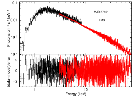
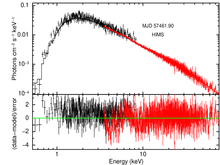
The first three observations (i.e. days 9, 14, 16) suggest that (see Table 3) a high energy cut-off is required for the spectral fits during the rising phase of the outburst. The value of cut-off indicates a decreasing trend from $228^{+72}_{-44}$ keV to $98^{+12}_{-9}$ keV as the source transits from LHS to HIMS. The left panel of Figure 8 shows the phenomenological modelling of the broadband observation on day 16 (MJD 57461). The spectra on day 89 (MJD 57534; SIMS decay) also shows a weak signature of a cut-off. It should be noted that the cutoffpl is given by $A(E)=KE^{-\alpha}exp(-E/\beta)$ where $\alpha$ is powerlaw photon index, $\beta$ is the high energy cut-off in keV and K is the normalization. There is no restriction on the value of $\beta$. At $\beta=\infty$ we get back the normal powerlaw, $A(E)=KE^{-\alpha}$ . From Table 6 it is clear that the improvement in $\chi^{2}$/dof is significantly larger in HIMS than in LHS when we use a cutoffpl. This is because a larger high energy cut-off value results in a smaller deviation from the normal powerlaw within the instrument energy range.

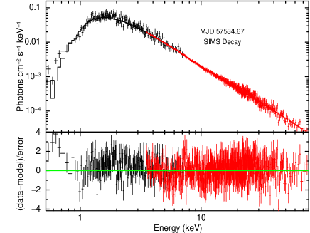
Table 3 shows that a reflection component is required for the observations on days 9 (MJD 57454), 14 (MJD 57459), 16 (MJD 57461) and 31 (MJD 57476). Besides this we see a trend in the evolution of photon index from 1.58$\pm{0.028}$ in the LHS to 2.41$\pm{0.01}$ in the HSS. And then the photon index reduces to 2.03$\pm{0.032}$ as the source enters the decay phase SIMS. Thus the state evolution is quite obvious from the broadband observations itself. It is also observed that the presence of disc component has begun from rising phase SIMS on day 31 (MJD 57476) at a Tin of 0.59 keV and it increased to 1.06 keV during the HSS. The phenomenological modelling corresponding to HSS is shown in the right panel of Figure 8. The presence of strong thermal emission during the HSS is evident from this figure as discussed earlier. In the next sub section we use a spectral model based on the two-component accretion flow to study the spectra and estimate accretion parameters for each state of the system.

Table 3 : Broadband phenomenological fit parameters using the model phabs(diskbb+ireflect*cutoffpl)

MJD	Observatory	Tin	$rel\_refl$	Photon Index	high-cut (keV)	$\chi^{2}$/dof
57454 (LHS)	NuSTAR	$-$	$0.39^{+0.06}_{-0.06}$	$1.58^{+0.028}_{-0.028}$	$228^{+72}_{-44}$	1011.08/986=1.02
57459 (LHS$>$HIMS)	NuSTAR+XRT	$-$	$0.27^{+0.07}_{-0.06}$	$1.55^{+0.02}_{-0.02}$	$117^{+18}_{-14}$	1234.81/1218=1.01
57461 (HIMS)	NuSTAR+XRT	$-$	$0.34^{+0.07}_{-0.07}$	$1.58^{+0.020}_{-0.019}$	$98^{+12}_{-09}$	1202.27/1113=1.08
57476 (SIMS)	NuSTAR	$0.59^{+0.014}_{-0.015}$	$0.60^{+0.07}_{-0.08}$	$2.41^{+0.017}_{-0.020}$	$-$	909.25/811=1.12
57508 (HSS)	NuSTAR+XRT	$1.06^{+0.006}_{-0.006}$	$-$	$2.41^{+0.01}_{-0.01}$	$-$	967.07/966=1.00
57534 (SIMS decay)	NuSTAR+XRT	$1.06^{+0.022}_{-0.024}$	$-$	$2.03^{+0.032}_{-0.032}$	$262^{+58}_{-40}$	970.46/943=1.02

4.4 Modeling with two component accretion flow

4.4.1 Model description

In this paper, we attempt to model the energy spectra of 2016 outburst of the source using the two component accretion flow paradigm (Chakrabarti & Titarchuk, 1995; Mandal & Chakrabarti, 2005; Iyer et al., 2015). The model considers two components - a Keplerian disc (Shakura & Sunyaev, 1973) at the equatorial plane which produces the soft photons, and a sub-Keplerian halo on top and bottom of the Keplerian disc. The sub-Keplerian flow close to the central object creates an effective boundary in presence of shocks (Chakrabarti, 1996; Chakrabarti & Das, 2004; Das, 2007; Chattopadhyay & Chakrabarti, 2011). Or else it forms a pileup of matter due to centrifugal barrier. This central region acts as the Compton corona/clouds, which inverse-Comptonizes the soft photons producing the high energy emission. In this model the total radiation spectrum is calculated self-consistently from hydrodynamics. Therefore, the low energy soft photons from Keplerian disc and Comptonized components (high energy) are not independent like phenomenological models ($diskbb+powerlaw$).

The two component flow model consists of four parameters, namely, shock location ($r_{s}$ in units of $r_{g}=2GM/c^{2}$) which represents the size of the Compton corona, Keplerian disc rate ($\dot{m}_{d}$) and sub-Keplerian halo accretion rate ($\dot{m}_{h}$) in units of $\dot{m}_{Edd}$ and mass (M) of the BH in units of solar mass M_☉. Earlier, we have imported the radiation spectra generated from two component advective model as a local additive model into XSpec using $atable$ command and fitted the broad-band spectral data in the range of 0.5 - 100 keV (see Iyer et al. 2015 and references therein for details) for the 2011 outburst of IGR J17091$-$3624. Following similar methodology, here, we perform broad-band spectral modelling (0.5 - 79 keV) using XSpec, of four quasi-simultaneous observations during the 2016 outburst of IGR J17091$-$3624 using Swift and NuSTAR data. In order to get error estimates for the parameters of the table model, we use the Migrad method.

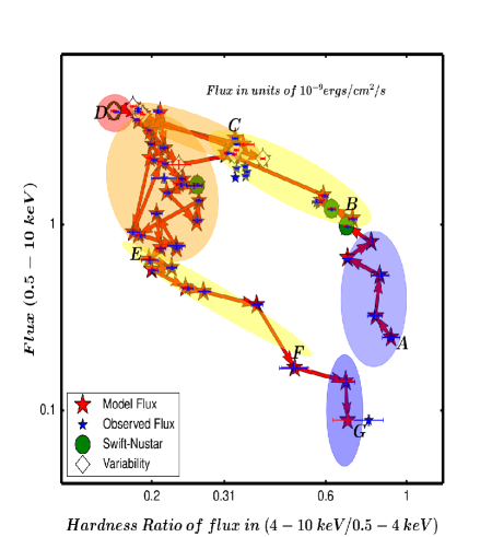
Once we obtain satisfactory fits and error ranges, we compute the unabsorbed flux values corresponding to the model using $cflux$ command. We estimate the unabsorbed fluxes in two different energy ranges 0.5 - 4 keV and 4 - 10 keV, for all 51 SWIFT-XRT observations modelled with two component flow. Then we take the ratio of flux in 4 - 10 keV to flux in 0.5 - 4 keV to obtain the hardness ratio. The plot of total flux versus hardness ratio for two component flow is shown in Figure 13 in red stars. On the same figure we over-plot the total flux versus hardness ratio as obtained from the phenomenological model in blue stars for the sake of comparison.

According to two component flow model, a source enters into outburst with significantly larger halo accretion rate than the Keplerian disc accretion rate. As the outburst progresses in the rising phase, the Keplerian disc starts contributing to the source luminosity and sub-Keplerian matter becomes less important. In the dynamical process of evolution, the corona cools down and shrinks in size as the outburst progresses. During the peak of the outburst, the Keplerian disc is prominent and hence the disc accretion rate is higher than before. A reverse trend occurs in the declining phase of the outburst.

Below we summarize the modelling of the broad-band observations using this two component flow model, and evolution of the different parameters. We also give an account of the source mass estimation performed using the same model.

Fig. 9 : Modeling of broad-band energy spectra (0.5 - 79 keV) using the two component advective flow model for different spectral states in the order of LHS to HIMS transition, HIMS, HSS for rising phase and SIMS of decay phase. Swift-XRT data is shown with black points, and NuSTAR data is shown with red points. See text for details.

4.4.2 Broad-band energy spectra and mass estimation

We model all six NuSTAR observations with the two component accretion flow model. Four of these are broadband observations were we have quasi-simultaneous XRT observations also. An additional model component $highecut$ is required only during the HIMS in-order to model the high energy cutoff with cut-off energy 121 keV. The requirement of a high energy cut-off is related to the way the two component flow model addresses the reflection contribution. In this model, the reflection contribution is calculated (Chakrabarti & Titarchuk, 1995) based on analytical solution of Fokker-Planck equation (following Sobolev 1975) which gives asymptotic results. A Montecarlo calculation is required to address more general situations. The reflection estimation in two component model works fine when the reflection contribution is moderate. So here we find that the model is able to fit all the data sets except one data set. For this particular data set a strong reflection component is required and hence the required e-folding energy is lower than the same calculated from the model. Hence we require an additional high energy cutoff component while performing the analysis. Usually we find that a smedge component alone is required for the fits along-with the two component flow model.

For the spectral fitting we use a fixed n_H value of $1.1\times 10^{22}$ atoms cm^-2. For the HSS we required the introduction of an additional pcfabs component that takes care of the partial covering fraction absorption. The covering fraction for this observation is 0.87 and pcfabs has an n_H value of $1.16\times 10^{22}$ atoms cm^-2. This indicates the presence of winds in the system (Savolainen, 2012; Koljonen et al., 2013; Radhika et al., 2016b; Pahari et al., 2017). The model fitted broad-band spectra for different states (see section 4.1 and yellow stars in Figure 4) during the outburst evolution are shown in Figure 9. In this figure, SWIFT data is plotted in black and NuSTAR data is plotted in red color. We then estimate the model parameters with $90\%$ confidence using Migrad method as mentioned earlier and the results are summarized in Table 4.

Table 4 : Broadband fit parameters and chi squared values obtained using two component flow model.

MJD	Observatory	Mass ($M_{\odot})$	halo rate $(\dot{M}_{Edd})$	disk rate $(\dot{M}_{Edd})$	$\chi^{2}$/dof
57454 (LHS)	NuSTAR	$11.66\pm 0.12$	$0.36\pm 0.002$	$0.04\pm 0.0006$	1183.82/987=1.19
57459 (LHS$>$HIMS)	NuSTAR+XRT	$11.27\pm 0.21$	$0.31\pm 0.0007$	$0.04\pm 0.001$	1278.28/1089=1.17
57461 (HIMS)	NuSTAR+XRT	$11.70\pm 0.13$	$0.30\pm 0.005$	$0.04\pm 0.001$	1253.43/1100=1.13
57476 (SIMS)	NuSTAR	$11.51\pm 0.07$	$0.10\pm 0.0007$	$0.31\pm 0.009$	1037.44/810=1.28
57508 (HSS)	NuSTAR+XRT	$11.12\pm 0.10$	$0.08\pm 0.0004$	$0.39\pm 0.010$	1042.14/963=1.08
57534 (SIMS decay)	NuSTAR+XRT	$10.93\pm 0.10$	$0.10\pm 0.0004$	$0.32\pm 0.004$	950.24/855=1.11

In two-component model, the mass and the accretion rates of the source self-consistently determine the density and temperature distribution of the flow. This in turn estimates the spectral signatures like fraction of inverse-Comptonized black body photons, energy spectral index etc. So, the model must choose the correct mass of the source to match all the spectral features found in different observed data sets. The model normalization is just a constant scaling factor. The overall normalization, $N\propto cos(i)/D^{2}$, depends on the inclination angle $(i)$ of the disc normal to the observer and the distance (D expressed in unit of 10 kpc) to the source. We can not fix the value of $N$ since both $i$ and D are unknown. But we have to choose a constant $N$ if we wish to estimate the mass of the source consistently across all observations.

It has to be specifically noted that we do not assume any particular value of $D$ or $i$ in our calculation. We have rather adopted the following procedure to fix the value of $N$. First, we fit all the broadband data sets keeping $N$ as a free parameter until we get the best fit. From this we find the range $N_{min}<N<N_{max}$, where $N_{min}=1.5$, $N_{max}=4.27$ corresponds to different data sets. Then we refit all the four broadband spectra with normalization frozen to the mean value $(N_{av}=2.885)$ obtained from these four observations and use this result to estimate the mass of the source. Normalization, in principle, can be any constant value between $N_{min}-N_{max}$ and different values of $N$ in the range can cause variations in the estimated mass. We have taken this systematic effect in our calculation as well.

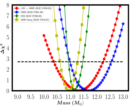
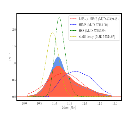
Once we obtain satisfactory fits for the all four broad-band energy spectra with $N=N_{av}$, the steppar command is used to obtain the $\Delta\chi^{2}$ values as a function of mass parameter in all four cases. This is plotted in Figure 10, where red, blue, green and yellow curves represent LHS, HIMS, HSS and SIMS (decay) spectral states respectively. Then, we convert the confidence intervals (as obtained by steppar) to probability distribution functions (PDF) using the steps followed in Iyer et al. (2015). The probability distribution functions are plotted in Figure 11 for all four observations with the same colour references as in 10. The PDFs are then combined (shown as “SUM PDF” in Fig. 11) by summing the four PDFs to obtain the lower and upper limits on mass from the four observations.

In order to estimate the effect of arbitrariness in the normalization values on mass, the process mentioned above for $N_{av}$ is repeated for the different values of $N$ in the range $N_{min}-N_{max}$. Then, we get the combined PDF in this case (shown as “SUM PDF (with systematics)” in Fig. 11) by summing all PDFs having different constant $N$ values. We see that it does not differ much from the combined PDF (blue shaded curve) for $N_{av}$. Hence it shows that the arbitrariness of the normalization value on the estimated mass is minimal. The mass range for 90% confidence level is between 10.65 - 12.24 M_⊙ for average norm. The same including systematic lies in the range 10.62 - 12.33 M_⊙. It is noted that in this method the mass of the source can be directly estimated from the fitting process as an independent fit parameter. Also the estimated mass is not very much dependent on the normalization, inclination angle and distance to the source.

Fig. 10 : $\Delta\chi^{2}$ versus mass of the source during the different spectral states obtained from $steppar$ command output in XSpec are shown for the mean norm value of 2.885 (see text for details)

.

Fig. 11 : PDFs obtained from $\Delta\chi^{2}$ confidence curves for four broadband spectra. The blue shaded curve with “SUM PDF” represents the combined PDF by summing all four PDFs with $N_{av}$ whereas the red shaded curve shows the combined PDF obtained by considering various normalizations between $N_{min}$ and $N_{max}$. The 90% mass range is between $10.62-12.33M_{\odot}$.

4.4.3 Evolution of model parameters and ‘q’-profile

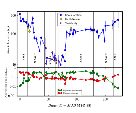
In Figure 12, we show the variation of shock location (size of Compton cloud) and accretion rates (Keplerian and sub-Keplerian). The state transitions are marked with vertical lines during the 2016 outburst. Figure 13 represents the evolution of total flux in the range of 0.5 - 10 keV with respect to the hardness ratio based on two component flow model. Below we give the values of different parameters of our physical model. The units for each of these parameters are given in section 4.4.1.

During the initial few days of the outburst, we find that the source is in the LHS as shown in blue patch in Figure 13. In the LHS the shock location varies from $r_{s}=450$ to $r_{s}=157$ and the halo rate is at its highest with a value of $\dot{m}_{h}=0.36$. Whereas the disk rate in LHS is only $\dot{m}_{d}=0.01-0.07$. As the system enters the HIMS (identified by yellow patch in Figure 13) the disk rate increases and exceeds the halo rate and the shock location gradually decreases. Here the Keplerian accretion rate reaches up to an average value of $\dot{m}_{d}=0.25$ and $\dot{m}_{h}$ ranges from $0.20$ to $0.09$.

After the HIMS the state of the system changes to SIMS where the shock location suddenly decreases and settles to a mean value $r_{s}=20$. This indicates that the post-shock region (i.e. Comptonized corona) is smaller in size and hence the contribution of hard photons is less. In the SIMS the disk accretion rate has an average value $\dot{m}_{d}=0.23$ while $\dot{m}_{h}=0.09$. Variabilities are observed in this state (see Figure 7) and model fitted parameters during these variabilities are marked with magenta coloured diamonds in Figure 12 and with white diamonds in the ‘q’-plot (Figure 13). It is clear from the ‘q’-plot that during these variabilities the source does not show any significant change in the flux values.

Then the system reaches the end of the rising phase by entering into the HSS. In the HSS the shock location is a low value of $r_{s}=14$. This implies that the disk is more dominant than the halo, with the disk accretion rate $\dot{m}_{d}=0.39$ and a low $\dot{m}_{h}=0.08$. The corresponding point is marked with a red patch in Figure 13.

Following the HSS is the decay phase wherein the state change from SIMS to HIMS and finally to LHS. In the SIMS decay phase (orange patch as shown in Figure 13) the accretion rate remains almost constant while the shock location abruptly goes up to around $r_{s}=100$. In the HIMS decay phase the shock location gradually starts rising to $r_{s}=201$. Here the halo rate remains constant but the disk rate decreases from $\dot{m}_{d}=0.14$ to $\dot{m}_{d}=0.02$. The decay phase of HIMS is marked with transparent yellow coloured patch in Figure 13 extending from E to F. Finally in the LHS of the decay phase the shock location rises up-to $r_{s}=300$ and, $\dot{m}_{h}=0.19$ exceeds the disc accretion rate $\dot{m}_{d}=0.007$.

Fig. 12 : Variation of shock location and accretion rates with time are plotted. The shock location decreases as the source transits from LHS to HSS and vice-versa. The halo accretion rate decreases whereas Keplerian accretion rate increases during rising phase and becomes comparable in the intermediate states before and after the HSS. In the decay phase both accretion rate show reverse behaviour. Data points corresponding to the four broad-band spectra that we have presented before are marked with yellow diamonds. The days when variability in SIMS is seen are marked with magenta diamonds.

Fig. 13 : HID showing the variation of total flux versus the ratio of flux in 4 - 10 keV to 0.5 - 4 keV obtained with two component advective model fitting. The LHS, HIMS, SIMS and HSS of rising and decay phase are shown with blue, yellow, orange and red patches respectively. See text for details.

5 Discussion and Conclusions

In this paper, we have studied the spectral and temporal variabilities of the black hole source IGR J17091$-$3624 during its 2016 outburst. It has been understood very well that based on the variations of the thermal and non-thermal emission, the BHs exhibit several spectral states and form a ‘q’-shaped HID profile. Several studies based on theoretical models have looked into these, and explored the accretion phenomenon (Belloni et al. 2005; Dunn et al. 2010; Nandi et al. 2012; Radhika & Nandi 2014 and references therein). The two component advective flow model (Chakrabarti & Titarchuk, 1995) suggests that the thermal emission is occurring from the Keplerian flow. The sub-Keplerian corona inverse Comptonize the soft photons resulting in a power-law hard photons distribution. Depending upon the contribution from Keplerian and sub-Keplerian flow during the accretion process, BH sources occupy the different spectral states. Based on this understanding of the accretion phenomenon, in this paper we have looked into the evolution of spectral and temporal characteristics of IGR J17091$-$3624 during its recent outburst in 2016.

We find that during the rising phase of the outburst, the source occupies hard and hard intermediate states. During the hard state, the source exhibits a powerlaw spectrum with the hardness ratio $\sim$0.9 and high fractional rms variability in the PDS (as shown in Table 1, Figure 4). The broad-band fit using two component flow model implies that the values of shock location and sub-Keplerian halo rate are maximum (see Figure 12). In the HIMS, the contribution of thermal emission increases. This is also evident in the decrease of both the hardness ratio and fractional rms variability (right panel of Figure 4). The shock location and halo rate have decreased while the Keplerian disc accretion rate has increased. These factors suggest the rise of thermal emission. Presence of reflection component at higher energies have been observed for a few observations in the LHS and HIMS of the rising phase (see also Xu et al. 2017). In addition to this, we find that the value of cut-off at high energies has a decreasing trend. This is similar to that observed in a few other black hole binaries like GX 339$-$4 (Motta et al., 2009).

An evolution of type C QPO frequencies is also observed from the LHS to HIMS. The QPOs observed in XRT data are weaker. But strong presence of QPOs are shown by NuSTAR observations (see Figure 6 and Table 2). Although Xu et al. 2017 has reported about the detection of QPOs in NuSTAR data of this outburst of the source, we understand that they have considered only observations belonging to the rising phase of the outburst. Here, in this manuscript we have found additional QPOs for many other observations and also the mHz QPOs which have not been discussed yet. In Sreehari et al. 2018 we have also further studied this evolution of QPOs using the propagating oscillation solution (Chakrabarti et al., 2008) of the two component flow model.

Following this, we find that the source enters the SIMS as evident in the decline of disc temperature, hardness ratio and fractional rms variability (see panel h of Figure 3 and right panel of Figure 4) w.r.t HIMS. Thus the emission is dominated by that due to the Keplerian disc. A higher ratio of Keplerian to halo accretion rate is observed (see Figure 12). For a very brief period on day 63 (MJD 57508), the source spectrum becomes softer with hardness ratio attaining its minimum value and also a lesser value of fractional rms variability (Figure 4). The spectral softening is also reflected in the increase of Keplerian disc accretion rate to a maximum of 0.39 M_Edd which is more than that during the SIMS-rise and decay phases. We understand that probably this short duration belongs to a HSS and this is unlike to typical BH sources (see Belloni et al. 2005; McClintock & Remillard 2006). The source later decays through the SIMS, HIMS and LHS, with a reverse trend of change in the Keplerian and halo accretion rates, and shock location. The outburst under consideration has a steep rise and exponential decay pattern. Hence the states in the decay phase persists for longer duration than the corresponding states in the rising phase.

Four broad-band XRT+NuSTAR observations (0.5 - 79 keV) have been modelled using two component model during different states of the outburst. It provides a better estimation of thermal and non-thermal contributions in the spectra. The behaviour of the model parameters are consistent with state transitions as mentioned before. Also they are found to be consistent with the values obtained by two component modelling of the XRT spectra alone (see Figure 12). Thus based on the phenomenological and two component model fits, we understand that the source occupies all the spectral states in the HID and completes the ‘q’-profile.

Previous publications have not been successful in producing a complete ‘q’-diagram for the 2011 outburst of the source. The only published paper which has shown a ‘q’-diagram is Capitanio et al. 2012 where the profile was incomplete since the study considered only till the HSS. The Astronomer’s Telegram by Pahari et al. 2012a, b discussed the source decaying towards its quiescence. But due to poor signal-to-noise ratio of the XRT data, they could not study the detailed spectral characteristics and hence the ‘q’-profile during decay phase. In this manuscript, for the 2016 outburst we have been able to understand that the source completes the ‘q’-diagram based on both phenomenological and two component flow modelling. This has been possible due to the XRT data having statistically significant count rate throughout the outburst unlike the 2011 outburst.

An interesting fact is that throughout the entire rising phase of the SIMS of the 2016 outburst, we observe variabilities/oscillations in the light-curve (see Figures 5 and 7) until the source entered the decay phase. The time period of oscillations suggest the presence of mHz QPOs. The extracted temporal data prove the existence of mHz QPOs for most of the days in the SIMS. Interestingly, all the observations with variability showed prominence of diskbb in the energy spectra for the phenomenological modelling. Higher Keplerian to halo accretion rate is also exhibited as compared to the other states (see bottom panel of Figure 12). This implies that the cause of the variability is essentially thermal in nature. Hence linked to the presence of a Keplerian disc that reaches close to the black hole. This is consistent with smaller values of shock location during this state (top panel of Figure 12). The signature of variabilities during day 46.54 of the SIMS has also been reported in an Astronomer’s Telegram by Reynolds et al. 2016. In 2011 outburst, similar oscillations were observed after the HSS only and existed for a long duration (Capitanio et al., 2012).

Apart from the variabilities during the SIMS, we observe weak signatures of variabilities during the transition from HIMS to SIMS, HSS and the initial days of SIMS-decay. There is no clear detection of variability in LHS possibly due to less source flux and hence is statistically insignificant. A weak 16 mHz QPO is observed in the NuSTAR observation during day 31.11 while the source is transiting from HIMS to SIMS. For the observation in HSS, both the XRT and NuSTAR PDS show broad QPO at 21.4 mHz and 20.7 mHz respectively. A very weak peaked component at 0.16 Hz is observed in the latter.

We would like to highlight that when we study outbursting sources as time dependent events, analytical models are not able to address the time evolution of the outbursting events similar to the variability signatures observed in this source. This is due to the fact that all analytical models are applicable in steady state situations only. Using numerical MHD simulations which include radiative cooling processes, might prove fruitful for this. In this paper we observed that the various types of heartbeat oscillations observed in this source are associated with intermediate states. According to two component flow model, the two types of accretion rate (Keplerian and sub-Keplerian) becomes comparable during the intermediate states. It might be possible that the radiation coupling between corona and with both types of flow (having different viscous time scale) may play a role to understand fast variabilities observed in this source. Detailed investigation of this feature using our model is at present beyond the scope of this paper.

The two component spectral modelling shows that the overall mass accretion rate is only 0.39 M_Edd during the HSS. Also, in section 4.1.4, we did find that the soft flux contribution to the entire spectra is only 33%. Thus the lack of Keplerian matter might be the reason for the source to occupy a short duration of HSS. This may not be allowing the source to be in HSS for a longer period of time before transitioning into the SIMS of the decay phase. All these factors indicate that possibly the outburst is triggered due to disc instability at the outer edge. And maybe a small amount of sub-Keplerian matter can be converted into the Keplerian matter (Mandal & Chakrabarti, 2010).

We also note that during the beginning of SIMS the spectral data extends only up-to 6 keV. This causes sudden absence of high energy flux suggesting that possibly a jet ejection has occurred. Unfortunately radio flares have not been observed as the system reaches the SIMS unlike the case in some outbursting sources (Fender et al., 2004, 2009; Miller-Jones et al., 2012; Radhika & Nandi, 2014; Radhika et al., 2016a).

By means of modelling the broad-band observations by SWIFT and NuSTAR X-ray observatories, we estimate the mass of the black hole candidate using the two component flow model. The range of values in which the mass varies is found to be 10.62 - 12.33 M_☉ including the systematic variation as mentioned earlier. This is consistent with the previous estimate of 11.8 - 13.7 M_☉ using similar methodology of spectral modelling by Iyer et al. 2015. It has to be clearly noted that in phenomenological models the parameters like T_in, powerlaw index are the distinct spectral signatures which can be tuned independently along with normalizations. In two-component model the parameters appear in hydrodynamic equations which self-consistently calculate the spectral features. This model has only one normalization and not separate normalizations as in diskbb and powerlaw. The advantage of this model is that mass and the accretion rate of the source self-consistently determine the density and temperature distribution of the flow. This in turn determine the spectral signatures like fraction of inverse-Comptonized black body photons, spectral index etc. So, the model chooses the correct mass of the source to match all the spectral features of all the data sets.

Thus from the phenomenological and two component accretion model fits, we can summarize the following points about the 2016 outburst of IGR J17091$-$3624.

• The source occupies all the spectral states and completes the ‘q’-profile in HID. Variation of parameters from phenomenological fits and two component model fits corroborate the same. Spectral state evolution based on correlation between the fractional rms variability and hardness ratio, is evident from the Hardness-RMS diagram.

• The halo accretion rate dominates during the hard and hard-intermediate states while the Keplerian - disc rate dominates the softer states.

• The size of the Compton corona (shock location) is minimum during the soft state and maximum during the LHS.

• Presence of reflection component due to ionized material, and decline in cut off energy are observed during the rising phase LHS and HIMS.

• An evolution of low frequency type C QPOs from 0.15 to 2.15 Hz is observed during the rising phase of LHS and HIMS. NuSTAR observations show strong signatures of QPOs during the LHS and HIMS.

• Coherent oscillations/variabilities are exhibited throughout the SIMS and also during the possible HSS. A very weak signature is seen during the transition from HIMS to SIMS in the rising phase. QPOs of the order of 20 mHz - 30 mHz are found during the SIMS. A 20.7 mHz broad QPO and a weak peaked component at 0.16 Hz exist during the possible HSS.

• Even in the presence of variabilities, the source completes the ‘q’-profile in its HID.

• Mass of the source is estimated to be in the range of 10.62 - 12.33 M_☉.

Acknowledgements We are thankful to the reviewer for his valuable comments and suggestions which have helped in improving the manuscript.

This research has made use of the data obtained through High Energy Astrophysics Science Archive Research Center on-line service, provided by NASA/GSFC.
RD is grateful to the support provided by the Vice Chancellor and Dean-SOE of DSU, and AN thanks GD, SAG; DD, PDMSA and Director, ISAC for encouragement and continuous support to carry out this research.

Appendix A Appendix

Table 5 : Log of SWIFT-XRT and NuSTAR observations considered for analysis

Observation ID		Date	Time	MJD	Exposure time
SWIFT	NuSTAR				(in sec)
00031921092		2016-02-27	08:24:58	57445.35	999.478
00031921093		2016-02-29	06:31:49	57447.27	994.458
00031921095		2016-03-03	22:40:19	57450.94	399.444
00031921097		2016-03-05	12:49:43	57452.53	849.457
	80001041002	2016-03-07	02:01:08	57454.08	43293
00031921101		2016-03-09	06:17:18	57456.26	1958.855
00031921104		2016-03-12	13:56:47	57459.58	1954.263
	80202014002	2016-03-12	14:11:08	57459.59	20238
00031921105		2016-03-13	17:14:59	57460.71	934.618
	80202014004	2016-03-14	19:26:08	57461.80	20698
00031921106		2016-03-14	21:43:26	57461.90	1049.610
00031921110		2016-03-20	21:09:58	57467.88	1004.331
00031921111		2016-03-21	00:39:40	57468.02	974.618
00031921112		2016-03-22	19:36:45	57469.81	1089.453
00031921113		2016-03-23	19:33:58	57470.81	849.447
00031921117		2016-03-27	14:25:14	57474.60	669.621
	80202014006	2016-03-29	02:41:08	57476.11	48393
00031921121		2016-04-01	20:11:58	57479.84	1044.448
00031921124		2016-04-04	16:46:58	57482.69	979.446
00031921132		2016-04-12	17:45:58	57490.74	904.443
00031921133		2016-04-13	13:05:46	57491.54	849.446
00031921134		2016-04-14	22:50:42	57492.95	849.617
00031921142		2016-04-23	15:27:58	57501.64	981.146
00031921143		2016-04-24	09:07:57	57502.38	964.443
00031921144		2016-04-27	18:34:58	57505.77	869.621
00031921145		2016-04-28	13:54:58	57506.57	979.313
	80202015002	2016-04-30	11:26:08	57508.47	39113
00081917001		2016-04-30	21:26:45	57508.89	1859.223
00031921147		2016-05-05	11:26:39	57513.47	789.447
00031921150		2016-05-08	19:30:58	57516.81	774.617
00031921153		2016-05-11	19:00:58	57519.79	974.617
00034543003		2016-05-13	07:35:58	57521.31	954.608
00034543006		2016-05-16	12:09:58	57524.50	959.607
00031921156		2016-05-16	18:31:57	57524.77	909.621
00034543009		2016-05-19	13:33:58	57527.56	984.609
00034543013		2016-05-24	21:17:58	57532.88	974.556
00031921160		2016-05-25	00:47:58	57533.03	504.441
	80202015004	2016-05-26	15:51:08	57534.66	36340
00081917002		2016-05-26	16:11:52	57534.67	1748.128
00031921161		2016-05-30	08:28:45	57538.35	249.606
00031921162		2016-05-31	01:51:29	57539.07	864.657
00031921163		2016-06-01	01:42:58	57540.07	924.617
00031921166		2016-06-04	01:26:57	57543.06	989.449
00031921170		2016-06-21	23:58:58	57560.99	1252.835
00031921173		2016-06-30	17:04:58	57569.71	364.461
00031921174		2016-07-02	20:01:58	57571.83	994.620
00031921175		2016-07-04	11:39:57	57573.48	1209.619
00031921176		2016-07-06	16:19:58	57575.68	919.784
00031921178		2016-07-11	17:32:58	57580.73	444.443
00031921179		2016-07-12	00:23:57	57581.01	1173.715
00031921180		2016-07-14	12:43:59	57583.53	1319.617
00031921183		2016-07-22	15:22:58	57591.64	1428.042
00031921184		2016-07-24	22:48:58	57593.95	969.272
00031921185		2016-07-26	11:39:57	57595.48	1439.619
00031921187		2016-08-12	00:51:57	57612.03	1519.016
00031921189		2016-08-17	19:41:58	57617.82	1559.234

Table 6 : Broadband fit models using various phenomenological models and corresponding $\chi^{2}$ values

MJD	Observatory	State	Model	$\chi^{2}/DOF$
57454	NuSTAR	LHS	phabs(powerlaw)	1221.16/990=1.23
			phabs(cutoffpl)	1198.05/989=1.21
			phabs(compTT)	1088.71/988=1.10
			phabs(ireflect*cutoffpl)	1011.10/987=1.02
			phabs(two-component)	1183.82/987=1.19
			phabs(smedge*two-component)	1131.39/985=1.14
			phabs(two-component*highecut)	1139.47/986=1.15
57459	NuSTAR+XRT	LHS$->$HIMS	phabs(powerlaw)	1405.42/1221=1.15
			phabs(cutoffpl)	1289.63/1220=1.05
			phabs(compTT)	1306.39/1219=1.07
			phabs(ireflect*cutoffpl)	1234.81/1218=1.01
			phabs(two-component)	1240.55/1087=1.14
			phabs(smedge*two-component)	1243.52/1086=1.14
			phabs(two-component*highecut)	1202.27/1086=1.08
57461	NuSTAR+XRT	HIMS	phabs(powerlaw)	1475.41/1116=1.32
			phabs(cutoffpl)	1290.67/1115=1.15
			phabs(compTT)	1328.03/1114=1.19
			phabs(ireflect*cutoffpl)	1202.27/1113=1.08
			phabs(two-component)	1567.62/1103=1.42
			phabs(smedge*two-component)	1534.64/1100=1.39
			phabs(two-component*highecut)	1227.02/1099=1.11
57476	NuSTAR	SIMS	phabs(diskbb+powerlaw)	1064.79/814=1.30
			phabs(diskbb+cutoffpl)	1084.38/813=1.33
			phabs(diskbb+compTT)	1047.77/812=1.29
			phabs(diskbb+ireflect*cutoffpl)	909.25/811=1.12
			phabs(two-component)	1667.30/814=2.04
			phabs(smedge*two-component)	1037.44/810=1.28
			phabs(smedge*smedge*two-component)	894.88/808=1.10
57508	NuSTAR+XRT	HSS	phabs(diskbb+powerlaw)	987.61/969=1.01
			phabs(diskbb+cutoffpl)	989.07/969=1.02
			phabs(diskbb+compTT)	996.02/967=1.03
			phabs(diskbb+ireflect*cutoffpl)	967.07/966=1.00
			phabs(smedge*two-component)	1558.65/967=1.61
			phabs(smedge*smedge*two-component)	1036.09/964=1.07
57534	NuSTAR+XRT	SIMS-decay	phabs(diskbb+powerlaw)	1000.36/946=1.06
			phabs(diskbb+cutoffpl)	1002.35/945=1.06
			phabs(diskbb+compTT)	1007.78/944=1.06
			phabs(diskbb+ireflect*cutoffpl)	970.46/943=1.02
			phabs(two-component)	1201.26/859=1.39
			phabs(smedge*two-component)	949.16/854=1.11

References

- Altamirano & Belloni (2012) Altamirano D., Belloni T., 2012, 747, L4
- Altamirano et al. (2011) Altamirano D., Belloni, T., Linares, M., et al. 2011, Astrophys. J. Lett., 742, L17
- Arnaud (1996) Arnaud K. A., 1996, in Jacoby G. H., Barnes J., eds, Astronomical Society of the Pacific Conference Series Vol. 101, Astronomical Data Analysis Software and Systems V. p. 17
- Belloni & Hasinger (1990) Belloni T. M., Hasinger G., 1990, Astron. Astrophys., 230, 103
- Belloni et al. (2001) Belloni T., Méndez M., Sánchez-Fernández C., 2001, 372, 551
- Belloni et al. (2005) Belloni T., Homan J., Casella P., et al., 2005, Astron. Astrophys., 440, 207
- Belloni et al. (2011) Belloni T. M., Motta S. E., Muñoz-Darias T., 2011, Bulletin of the Astronomical Society of India, 39, 409
- Brocksopp et al. (2002) Brocksopp C., Fender R. P., McCollough M., et al., 2002, Mon. Not. R. Astron. Soc., 331, 765
- Burrows et al. (2005) Burrows D. N., et al., 2005, 120, 165
- Capitanio et al. (2012) Capitanio F., Del Santo M., Bozzo E., Ferrigno C., De Cesare G., Paizis A., 2012, 422, 3130
- Capitanio et al. (2013) Capitanio F., Del Santo M., Bozzo E., Ferrigno C., De Cesare G., Paizis A., 2013, preprint, arXiv 1302.3485
- Casella et al. (2004) Casella P., Belloni T., Homan J., Stella L., 2004, Astron. Astrophys., 426, 587
- Chakrabarti (1996) Chakrabarti S. K., 1996, 464, 664
- Chakrabarti & Das (2004) Chakrabarti S. K., Das S., 2004, 349, 649
- Chakrabarti & Titarchuk (1995) Chakrabarti S., Titarchuk L., 1995, Astrophys. J., 455, 623
- Chakrabarti et al. (2008) Chakrabarti, S. K., Debnath, D., Nandi, A., & Pal, P. S. 2008, Astron. Astrophys., 489, L41
- Chattopadhyay & Chakrabarti (2011) Chattopadhyay I., Chakrabarti S. K., 2011, 20, 1597
- Chen et al. (1997) Chen W., Shrader C. R., Livio M., 1997, 491, 312
- Corral-Santana et al. (2016) Corral-Santana J. M., Casares J., Muñoz-Darias T., Bauer F. E., Martínez-Pais I. G., Russell D. M., 2016, 587, A61
- Court et al. (2016) Court J. M. C., Motta S. E., Altamirano D., 2016, The Astronomer’s Telegram, 8858
- Court et al. (2017) Court J. M. C., Altamirano D., Pereyra M., Boon C. M., Yamaoka K., Belloni T., Wijnands R., Pahari M., 2017, MNRAS, 468, 4748
- Das (2007) Das S., 2007, 376, 1659
- Dunn et al. (2010) Dunn R. J. H., Fender R. P., Körding E. G., Belloni T., Cabanac C., 2010, 403, 61
- Egron et al. (2016) Egron E., et al., 2016, The Astronomer’s Telegram, 8821
- Fender et al. (2004) Fender R. P., Belloni T., Gallo E., 2004, Mon. Not. R. Astron. Soc., 355, 1105
- Fender et al. (2009) Fender R. P., Homan J., Belloni T., 2009, Mon. Not. R. Astron. Soc., 396, 1307
- Greiner et al. (2016) Greiner J., Bolmer J., Gandhi P., Altamirano D., Charles P. A., Court J. M., Kann D. A., Walton D. J., 2016, The Astronomer’s Telegram, 8795
- Grinberg et al. (2016) Grinberg V., et al., 2016, The Astronomer’s Telegram, 8761
- Harrison et al. (2013) Harrison F. A., et al., 2013, 770, 103
- Homan & Belloni (2005) Homan J., Belloni T., 2005, Astrophys. Space Sci., 300, 107
- Homan et al. (2001) Homan J., Wijnands R., van der Klis M., Belloni T., van Paradijs J., Klein-Wolt M., Fender R., Méndez M., 2001, 132, 377
- Iyer & Nandi (2013) Iyer N., Nandi A., 2013, in Das S., Nandi A., Chattopadhyay I., eds, Astronomical Society of India Conference Series Vol. 8, Astronomical Society of India Conference Series. pp 79–83
- Iyer et al. (2015) Iyer N., Nandi A., Mandal S., 2015, 807, 108
- King et al. (2012) King A. L., et al., 2012, 746, L20
- Koljonen et al. (2013) Koljonen, K. I. I., McCollough, M. L., Hannikainen, D. C., & Droulans, R. 2013, Mon. Not. R. Astron. Soc., 429, 1173
- Krimm et al. (2011) Krimm H. A., et al., 2011, The Astronomer’s Telegram, 3144
- Kuulkers et al. (2003) Kuulkers E., Lutovinov A., Parmar A., Capitanio F., Mowlavi N., Hermsen W., 2003, The Astronomer’s Telegram, 149
- Kuznetsov et al. (1997) Kuznetsov S., et al., 1997, 292, 651
- Makishima et al. (1986) Makishima K., Maejima Y., Mitsuda K., et al., 1986, Astrophys. J., 308, 635
- Mandal & Chakrabarti (2005) Mandal S., Chakrabarti S. K., 2005, 434, 839
- Mandal & Chakrabarti (2010) Mandal S., Chakrabarti S. K., 2010, 710, L147
- McClintock & Remillard (2006) McClintock J. E., Remillard R. A., 2006, ‘Black hole binaries’, Compact Stellar X-ray sources, edited by Lewin W. H. G. and M. van der Klis
- Miller-Jones et al. (2012) Miller-Jones J. C. A., et al., 2012, 421, 468
- Miller et al. (2016) Miller J. M., Reynolds M., Kennea J., King A. L., Tomsick J., 2016, The Astronomer’s Telegram, 8742
- Mitsuda et al. (1984) Mitsuda K., et al., 1984, Publ. Astron. Soc. Jpn., 36, 741
- Motta et al. (2009) Motta S., Belloni T., Homan J., 2009, 400, 1603
- Motta et al. (2012) Motta S., Homan J., Munoz-Darias T., et al., 2012, Mon. Not. R. Astron. Soc., 427, 595
- Muno et al. (1999) Muno M. P., Morgan E. H., Remillard R. A., 1999, 527, 321
- Nandi et al. (2012) Nandi A., Debnath D., Mandal S., Chakrabarti S. K., 2012, Astron. Astrophys., 542, 56
- Pahari et al. (2012a) Pahari M., Bhattacharyya S., Yadav J. S., 2012a, The Astronomer’s Telegram, 4282
- Pahari et al. (2012b) Pahari M., Bhattacharyya S., Yadav J. S., 2012b, The Astronomer’s Telegram, 4283
- Pahari et al. (2014) Pahari M., Yadav J. S., Bhattacharyya S., 2014, 783, 141
- Pahari et al. (2017) Pahari, M., Antia, H. M., Yadav, J. S., et al. 2017, Astrophys. J., 849, 16
- Radhika & Nandi (2014) Radhika D., Nandi A., 2014, 54, 1678
- Radhika et al. (2016a) Radhika D., Nandi A., Agrawal V. K., Seetha S., 2016a, 460, 4403
- Radhika et al. (2016b) Radhika D., Nandi A., Agrawal V. K., Mandal S., 2016b, 462, 1834
- Rao & Vadawale (2012) Rao A., Vadawale S. V., 2012, 757, L12
- Rebusco et al. (2012) Rebusco P., Moskalik P., Kluźniak W., Abramowicz M. A., 2012, 540, L4
- Remillard & McClintock (2006) Remillard R. A., McClintock J. E., 2006, 44, 49
- Reynolds et al. (2016) Reynolds M., Miller J., King A., 2016, The Astronomer’s Telegram, 8948
- Rodriguez et al. (2011) Rodriguez J., Corbel S., Caballero I., Tomsick J. A., Tzioumis T., Paizis A., Cadolle Bel M., Kuulkers E., 2011, 533, L4
- Ross & Fabian (1993) Ross, R. R., & Fabian, A. C. 1993, Mon. Not. R. Astron. Soc., 261, 74
- Savolainen (2012) Savolainen, P. 2012, X-ray Binaries. Celebrating 50 Years Since the Discovery of Sco X-1, 52
- Shakura & Sunyaev (1973) Shakura N. I., Sunyaev R. A., 1973, Astron. Astrophys., 24, 337
- Sobolev (1975) Sobolev V. V., 1975, Light scattering in planetary atmospheres
- Sreehari et al. (2018) Sreehari, H., Nandi, A., Radhika, D., Iyer, N., & Mandal, S. 2018, Journal of Astrophysics and Astronomy, 39, #5
- Tanaka & Lewin (1995) Tanaka Y., Lewin W. H. G., 1995, X-ray Binaries, pp 126–174
- Tanaka & Shibazaki (1996) Tanaka Y., Shibazaki N., 1996, 34, 607
- Tetarenko et al. (2016) Tetarenko B. E., Sivakoff G. R., Heinke C. O., Gladstone J. C., 2016, 222, 15
- Tsunemi et al. (1989) Tsunemi H., Kitamoto S., Okamura S., Roussel-Dupre D., 1989, 337, L81
- Wilms et al. (2000) Wilms J., Allen A., McCray R., 2000, 542, 914
- Xu et al. (2017) Xu Y., et al., 2017, ApJ, 851, 103
- in’t Zand et al. (2003) in’t Zand J. J. M., Heise J., Lowes P., Ubertini P., 2003, The Astronomer’s Telegram, 160
- Zhang et al. (2014) Zhang, Z., Qu, J. L., Gao, H. Q., et al. 2014, Astron. Astrophys., 569, A33