A Linearized Viscous, Compressible Flow-Plate Interaction
with Non-dissipative Coupling

Abstract

We address semigroup well-posedness for a linear, compressible viscous fluid interacting at its boundary with an elastic plate. We derive the model by linearizing the compressible Navier-Stokes equations about an arbitrary flow state, so the fluid PDE includes an ambient flow profile $\mathbf{U}$. In contrast to model in [6], we track the effect of this term at the flow-structure interface, yielding a velocity matching condition involving the material derivative of the structure; this destroys the dissipative nature of the coupling of the dynamics. We adopt here a Lumer-Phillips approach, with a view of associating fluid-structure solutions with a $C_{0}$-semigroup $\left\{e^{\mathcal{A}t}\right\}_{t\geq 0}$ on a chosen finite energy space of data. Given this approach, the challenge becomes establishing the maximal dissipativity of an operator $\mathcal{A}$, yielding the flow-structure dynamics.

Keywords: fluid-structure interaction, compressible viscous fluid, plate, well-posedness, semigroup

AMS Mathematics Subject Classification 2010: 35A05, 74F10, 35Q35, 76N10

1 Introduction

In mathematical studies of fluid-structure interactions arising in application the effect of viscosity can be important. Indeed, viscous fluids introduce energy dissipation into the system, and produce non-trivial frictional effects in the interaction between fluid and solid. Interactive dynamics with viscous fluids are of paramount concern in the design and control of many physical systems [24], e.g., aircraft, buildings and bridges, gas pipelines, engines, as well as other applications such as blood flow in an artery (for instance see [12] and references therein). In such applications, the density of the flow may change along a streamline, and compressibility—the volume change per unit pressure change—becomes non-negligible.

In many scenarios, mathematical solution techniques and analytical frameworks can be greatly simplified by assuming the flow is inviscid—viscosity free. One of the principal motivating applications here is the field of aeroelasticity: elastic structures interacting with surrounding fluid flows, as with airfoils and paneling of aircraft. Typically, the compressible gas is assumed to be inviscid and the flow to be irrotational (inviscid potential flow) [24]. These assumptions reduce the flow dynamics to a perturbed wave equation [18, 24, 39]. Yet there are situations where viscous effects can simply not be neglected, e.g., for flows with Mach numbers$0.3<M<3$ [24, 26]. Moreover, in certain regimes or configurations viscous effects are paramount, e.g., the low-speed flapping flag problem [30, 1] or the transonic flow regime $(0.8<M<1.2)$ [24].

For incompressible flows, the analysis typically involves two unknowns: velocity and pressure (e.g., [13, 12, 19, 21]). One must solve both conservation of mass and linear momentum equations, with the fluid density constant. On the other hand, for compressible flow, density and pressure vary in the dynamics. Consequently, solutions in the compressible case require an equation of state for the fluid and a conservation of energy statement. Here, we will assume the pressure depends linearly on the density. (For more discussion on this point, see Section 2.)

In this paper we begin with a laminar, unperturbed flow of compressible fluid, and study perturbations about this given flow state. Such perturbations will be induced by a coupling to a non-stationary elastic dynamics imbedded in the fluid’s boundary. We restrict our attention to such flow-structure interactions where the fluid exists in a 3-D spatial domain, bounded by a 2-D Lipschitz domain. A flat portion of the boundary is the equilibrium state of an elastic plate—with dynamics dictated by a fourth order plate equation that neglects the effects of rotational inertia. The flow and structure are strongly coupled at the fluid-structure interface, with the plate dynamics affecting the flow through a normal component boundary condition, and the flow dynamics providing the dynamic distributed stresses across the surface of the plate. Taking the flow dynamics to be given by a linearization of compressible Navier-Stokes about a non-zero flow state $\mathbf{U}$ will turn out to have important repercussions in the interior (flow) dynamics, as well as at the flow-structure interface.

This problem is motivated by the main lines of the recent work of I. Chueshov et al. [15, 19, 20, 21] on various types of 3-D/2-D fluid-structure interactions (as considered here). In these papers, the authors address various combinations of viscous compressible and incompressible fluid dynamics in 3-D domains (sometimes unbounded but tubular [20]) linearized about the steady flow state $\mathbf{U}\equiv\mathbf{0}$, and coupled to different types of elastic dynamics at the interface (2-D in-plane elasticity [22], von Karman [21], or even full von Karman [19]). The Galerkin approach is utilized in constructing solutions, and dynamical systems techniques are used to obtain long-time behavior results for these systems. As a primary motivating reference, in [15], Chueshov considered the dynamics of a nonlinear plate, located on a flat portion of the boundary of a 3-D cavity, as it interacts with a compressible, isothermal fluid filling the cavity. There, the author addresses a natural first case of interest: $\mathbf{U}\equiv 0$, i.e., linearization about the trivial flow steady state. He shows both well-posedness and the existence of global attractors. In a personal correspondence with the authors of the present paper, Chueshov suggested that his method—based on a Galerkin approach with a priori energy estimates—would not accommodate the case of interest in aeroelasticity: linearization about $\mathbf{U}\neq\mathbf{0}$. Thus, he suggested the problem at hand as a problem of interest, and intimated that a Lumer-Philips (semigroup) approach might yield well-posedness.

In the present authors’ previous work [6], the suggested model was analyzed—that of [15]—with additional interior terms associated to the $\mathbf{U}\neq 0$. For this non-dissipative flow-structure model, a pure velocity matching condition was imposed at the interface. This type of coupling does not take into account flow effects at the interface with the plate arising from the presence of $\mathbf{U}\neq 0$. However, establishing well-posedness for the equations with a dissipative coupling already presented non-trivial technical challenges (discussed in detail in Section 4).

Viewing the work in [6] as a requisite preliminary step, the work at hand is the natural sequel in justifying and mathematically accommodating the non-dissipative coupling. The present paper carefully derives the fluid-structure interface conditions, which are necessarily non-dissipative due to $\mathbf{U}\neq\mathbf{0}$. Indeed, as with the fluid-structure models given in [8, 39, 17, 7], we do not have a “pure” velocity matching condition in the present work. Rather, we have an interface/coupling condition written also in terms of the material derivative of the structure, $(\partial_{t}+\mathbf{U}\cdot\nabla)w$. We critically use the techniques developed in [6] here, and the principal challenge is overcoming the addition of the non-dissipative coupling on the lower-dimensional interface.

1.1 Notation

For the remainder of the text we write $\mathbf{x}$ for $(x_{1},x_{2},x_{3})\in\mathbb{R}_{+}^{3}$ or $(x_{1},x_{2})\in\Omega\subset\mathbb{R}_{\{(x_{1},x_{2})\}}^{2}$, as dictated by context. For a given domain $D$, its associated $L^{2}(D)$ will be denoted as $||\cdot||_{D}$ (or simply $||\cdot||$ when the context is clear). The symbols $\mathbf{n}$ and $\mathbf{\tau}$ will be used to denote, respectively, the unit external normal and tangent vectors to $\mathcal{O}$. Inner products in $L^{2}(\mathcal{O})$ or $\mathbf{L}^{2}(\mathcal{O})$ are written $(\cdot,\cdot)_{\mathcal{O}}$ (or simply $(\cdot,\cdot)$ when the context is clear), while inner products $L^{2}(\partial\mathcal{O})$ are written $\langle\cdot,\cdot\rangle$. We will also denote pertinent duality pairings as $\left\langle\cdot,\cdot\right\rangle_{X\times X^{\prime}}$, for a given Hilbert space $X$. The space $H^{s}(D)$ will denote the Sobolev space of order $s$, defined on a domain $D$, and $H_{0}^{s}(D)$ denotes the closure of $C_{0}^{\infty}(D)$ in the $H^{s}(D)$-norm $\|\cdot\|_{H^{s}(D)}$ or $\|\cdot\|_{s,D}$. We make use of the standard notation for the boundary trace of functions defined on $\mathcal{O}$, which are sufficently smooth: i.e., for a scalar function $\phi\in H^{s}(\mathcal{O})$, $\frac{1}{2}<s<\frac{3}{2}$, $\gamma(\phi)=\phi\big{|}_{\partial\mathcal{O}},$ a well-defined and surjective mapping on this range of $s$, owing to the Sobolev Trace Theorem on Lipschitz domains (see e.g., [37], or Theorem 3.38 of [36]).

2 Flow and Interface Modeling

Let $\mathcal{O}\subset\mathbb{R}^{3}$ be a bounded and convex fluid domain (and so has Lipschitz boundary $\partial\mathcal{O}$; see e.g., Corollary 1.2.2.3 of [29]). The boundary decomposes into two pieces $\overline{S}$ and $\overline{\Omega}$ where $\partial\mathcal{O}=\overline{S}\cup\overline{\Omega}$, with $S\cap\Omega=\emptyset$. We consider $S$ to be the solid boundary, with no interactive dynamics, and $\Omega$ to be the equilibrium position of the elastic domain, upon which the interactive dynamics take place. We also assume that: (i) the active component $\Omega\subset\mathbb{R}^{2}$ is flat, with $C^{2}$ boundary, and embedded in the $x_{1}$–$x_{2}$ plane; (ii) the inactive component $S$ lies below the $x_{1}$–$x_{2}$ plane. This is to say,

$$\Omega\subset ~{}\{\mathbf{x}=(x_{1},x_{2},0)\}$$ (2.1)

$$S\subset ~{}\{\mathbf{x}=(x_{1},x_{2},x_{3})~{}:~{}x_{3}\leq 0\}.$$ (2.2)

We denote the unit outward normal vector to $\partial\mathcal{O}$ by $\mathbf{n}(\mathbf{x})$ where $\left.\mathbf{n}\right|_{\Omega}=[0,0,1],$ as in Figure 1 and the unit outward normal vector to $\partial\Omega$ by $\mathbf{\nu}(\mathbf{x})$.

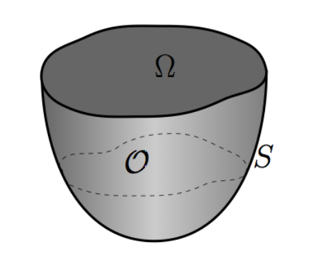
Figure 1: The Fluid-Structure Geometry

Suppose the domain $\mathcal{O}$ is filled with fluid whose governing dynamics are the compressible Navier–Stokes system [26, 14] (see also [22]). We then linearize this model with respect to a reference state $\{{\varrho}_{*};\mathbf{U};p_{*}\}$, and suppose that the unperturbed flow $\mathbf{U}:\mathcal{O}\rightarrow\mathbb{R}^{3}$ is given by:

$$\mathbf{U}(x_{1},x_{2},x_{3})=[U_{1}(x_{1},x_{2},x_{3}),U_{2}(x_{1},x_{2},x_{3}),U_{3}(x_{1},x_{2},x_{3})],$$ (2.3)

and represents a mild (time-independent) ambient fluid flow. The quantities ${\varrho}_{*},p_{*}$ are taken to be constant in time. Then, for small perturbations $\{\rho;\mathbf{u};p\}$ of this ambient state, we write

$$\tilde{\rho}=~{}\rho_{*}+\rho,~{}~{}~{}~{}~{}\tilde{p}=~{}p_{*}+p,~{}~{}~{}~{}~{}\tilde{\mathbf{u}}=~{}\mathbf{U}+\mathbf{u}.$$

At this point, we assume the pressure is a linear function of the density. This assumption can be arrived at in two ways, which we now briefly describe:

For isentropic flows, the relationship between pressure and density is (see, e.g., [26, 40, 23])

$$\tilde{p}=C[\tilde{\rho}]^{\gamma},$$ (2.4)

where $C$ is a constant evaluated for the pressure and density in the far field and $\gamma>0$—for air, $\gamma=1.4$. (We note that isentropic flows [24, pp.169–200] are barotropic—i.e., pressure depending only on density.) Equation (2.4) can be linearized through the above perturbation convention, taking $p_{*}$ and $\rho_{*}$ to be the far field pressure and density, yielding the linear relation

$${p}=C\big{(}\gamma,{\rho_{*}},{p_{*}}\big{)}{\rho}.$$ (2.5)

On the other hand, if one considers isothermal flow, the ideal gas law reads: $\tilde{p}=\tilde{\rho}RT$, where $T$ is the temperature and $R$ is a fluid-dependent constant. This equation also presents a linear relation between pressure and density, if $T$ is a constant. Isothermal flows are used in low speed situations, i.e., with velocities much less than the speed of sound. Isentropic flow is used for compressible flows with small viscosity, and the ideal gas law is used for compressible viscous flows. We do note that $T$ is typically taken as an unknown for compressible viscous flows; if this consideration is made, an energy balance equation is required.

Remark 2.1.

Note that our assumption of linear pressure-density dependence could possibly be weakened in the analysis. In this case, we would take the flow to be isentropic as in [40, 23], though, in these references the problem is entirely stationary. With this assumption, the flow coupling is inherently nonlinear, introducing additional complexity into the analysis [26]. We view the analyses in [6] and here as first steps, noting that the linear flow problem here is already of great technical complexity and mathematical challenge. We note the more recent references [9, 28], each of which focuses on the issue of weak solvability for certain nonlinear, compressible, viscous fluid-structure interactions.

For mathematical simplicity we now take $p=\rho$ and assume $p_{*}={\varrho}_{*}=1$. If we generalize the forcing functions, then we obtain the physical perturbation equations:

$$(\partial_{t}+\mathbf{U}\cdot\nabla)p+{\mathrm{d}iv\,}\,\mathbf{u}+(\text{div}~{}\mathbf{U})p=f(\mathbf{x})\quad{\mathrm{i}n}~{}~{}\mathcal{O}\times\mathbb{R}_{+},$$ (2.6a)

$$(\partial_{t}+\mathbf{U}\cdot\nabla)\mathbf{u}-\nu\Delta\mathbf{u}-(\nu+{\lambda}){\nabla}{\mathrm{d}iv\,}\,\mathbf{u}+{\nabla}p+\nabla\mathbf{U}\cdot\mathbf{u}+(\mathbf{U}\cdot\nabla\mathbf{U})p=\mathbf{F}(\mathbf{x})\quad{\mathrm{i}n}~{}\mathcal{O}\times\mathbb{R}_{+},$$ (2.6b)

where the dynamic viscosity of the fluid is given by $\nu>0$, and $\lambda\geq 0$ is Lamé’s first parameter (both of which would vanish in the case of inviscid fluid). Given the Lamé Coefficients, the stress tensor $\sigma$ of the fluid is defined as

$$\sigma(\mathbf{\mu})=2\nu\epsilon(\mathbf{\mu})+\lambda[I_{3}\cdot\epsilon(\mathbf{\mu})]I_{3},$$

where the strain tensor $\epsilon$ is given by

$$\epsilon_{ij}({\mathbf{\mu}})=\dfrac{1}{2}\left(\frac{\partial\mu_{j}}{\partial x_{i}}+\frac{\partial\mu_{i}}{\partial x_{j}}\right)\text{, \ }1\leq i,j\leq 3.$$

With this notation it is easy to see that

$$\text{div}~{}\sigma(\mathbf{\mu})=\nu\Delta\mathbf{\mu}+(\nu+\lambda)\nabla\text{div}(\mathbf{\mu}).$$

While the linearized interior terms are by now tractable [6], we must supply the fluid equation with the correct boundary conditions on $\partial\mathcal{O}$ that will necessarily involve the plate’s deflections $w$ on $\Omega\subset\partial\mathcal{O}$. The full system (with structural equations) will be discussed in detail in the following section; here, we impose the so called impermeability condition on $\Omega$, namely, that no fluid passes through the elastic portion of the boundary during deflection [8, 24].

Let $S(a_{1},a_{2},a_{3})=0$ describe the interface in Lagrangian coordinates in $\mathbb{R}^{3}$; also let ${\mathbf{x}}=[x_{1},x_{2},x_{3}]$ be the Eulerian position inside $\mathcal{O}$. Then, letting $w(x_{1},x_{2},t)$ represent the transverse ($x_{3}$) displacement of the plate on $\Omega$, we have that

$$S\big{(}x_{1},x_{2},x_{3}-w(x_{1},x_{2};t)\big{)}\equiv\mathscr{S}(x_{1},x_{2},x_{3};t)=0,$$

describes the time-evolution of the boundary. The impermeability condition requires that the material derivative ($\partial_{t}+\tilde{\mathbf{u}}\cdot\nabla_{\mathbf{x}}$) vanishes on the deflected surface [8, 14, 24]:

$$\big{(}\partial_{t}\mathcal{+}\tilde{\mathbf{u}}\cdot\nabla_{\mathbf{x}}\big{)}\mathscr{S}=0,~{}~{}~{}~{}~{}\tilde{\mathbf{u}}=\mathbf{u}+\mathbf{U}$$

Applying the chain rule, we obtain

$$\nabla_{\mathbf{x}}S\cdot[0,0,-w_{t}]+\mathbf{U}\cdot\big{(}\nabla_{\mathbf{x}}S+[-S_{x_{3}}w_{x_{1}},-S_{x_{3}}w_{x_{2}},0]\big{)}=-\mathbf{u}\cdot\big{(}\nabla_{\mathbf{x}}S+[-S_{x_{3}}w_{x_{1}},-S_{x_{3}}w_{x_{2}},0]\big{)}.$$ (2.7)

We identify $\nabla_{\mathbf{x}}S$ as the normal to the deflected surface; assuming small deflections and restricting to $(x_{1},x_{2})\in\Omega$, we can identify $\nabla_{\mathbf{x}}S\big{|}_{\Omega}$ with $\mathbf{n}\big{|}_{\Omega}=[0,0,1]$. Making use of (2.7), imposing that $\mathbf{U}\cdot\mathbf{n}=0$ on $\partial\mathcal{O}$ (see (5.1) and discussion), and discarding quadratic terms, this relation allows us to write for $(x_{1},x_{2})\in\Omega$:

$$\mathbf{n}\cdot[0,0,w_{t}]+\mathbf{U}\cdot[w_{x_{1}},w_{x_{2}},0]=\mathbf{u}\cdot\mathbf{n}.$$

This yields the desired flow boundary condition for the dynamics:

$$\mathbf{u}\cdot\mathbf{n}\big{|}_{\Omega}=w_{t}+\mathbf{U}\cdot\nabla w.$$ (2.8)

3 Main Flow-Structure PDE Model

Deleting non-critical lower order and the benign inhomogeneous terms in (2.6a)-(2.6b) (see also [6]), we obtain the essential perturbation equations to be studied below:

$$\left\{\begin{array}[]{l}p_{t}+\mathbf{U}\cdot\nabla p+\text{div}~{}\mathbf{u}=0~{}\text{ in }~{}\mathcal{O}\times(0,\infty)\\[1.42271pt] \mathbf{u}_{t}+\mathbf{U}\cdot\nabla\mathbf{u}-\text{div}~{}\sigma(\mathbf{u})+\eta\mathbf{u}+\nabla p=0~{}\text{ in }~{}\mathcal{O}\times(0,\infty)\\[1.42271pt] [\sigma(\mathbf{u})\mathbf{n}-p\mathbf{n}]\cdot\bm{\tau}=0~{}\text{ on }~{}\partial\mathcal{O}\times(0,\infty)\\[1.42271pt] \mathbf{u}\cdot\mathbf{n}=0~{}\text{ on }~{}S\times(0,\infty)\\[1.42271pt] \mathbf{u}\cdot\mathbf{n}=w_{t}+\mathbf{U}\cdot\nabla w~{}\text{ on }~{}\Omega\times(0,\infty)\end{array}\right.$$ (3.6)

$$\left\{\begin{array}[]{l}w_{tt}+\Delta^{2}w+\left[2\nu\partial_{x_{3}}(\mathbf{u})_{3}+\lambda\text{div}(\mathbf{u})-p\right]_{\Omega}=0~{}\text{ on }~{}\Omega\times(0,\infty)\\[1.42271pt] w=\nabla w\cdot\mathbf{\nu}=0~{}\text{ on }~{}\partial\Omega\times(0,\infty)\end{array}\right.$$ (3.9)

$$\begin{array}[]{c}\left[p(0),\mathbf{u}(0),w(0),w_{t}(0)\right]=\left[p_{0},\mathbf{u}_{0},w_{0},w_{1}\right].\end{array}$$ (3.11)

Here, $p(t):\mathbb{R}^{3}\rightarrow\mathbb{R}$ and $\mathbf{u}(t):\mathbb{R}^{3}\rightarrow\mathbb{R}^{3}$ (pointwise in time) are given as the (Eulerian) pressure and the fluid velocity field, respectively. The quantity $\eta>0$ represents a drag force of the domain on the viscous fluid. The function $w(t):\mathbb{R}^{2}\to\mathbb{R}$ gives the transverse deflection of points $\mathbf{x}\in\Omega$, evolving according to a plate equation. In addition, the given quantity $\mathbf{\tau}$ in (3.6) is in the space $TH^{1/2}(\partial\mathcal{O)}$ of tangential vector fields of Sobolev index 1/2; that is,

$$\mathbf{\tau}\in TH^{1/2}(\partial\mathcal{O)=}\{\mathbf{v}\in\mathbf{H}^{\frac{1}{2}}(\partial\mathcal{O})~{}:~{}\mathbf{v}\cdot\mathbf{n}=0~{}\text{ on }~{}\partial\mathcal{O}\}.$$ (3.12)

Remark 3.1.

For convenience, we will refer to the fluid boundary condition on $\Omega$

$$\mathbf{u}\cdot\mathbf{n}=w_{t}+\mathbf{U}\cdot\nabla w$$ (3.13)

as the coupling condition.

The boundary conditions invoked in (3.6) are the so-called impermeability-slip conditions [8, 14]. As discussed above, the physical interpretation is that no fluid passes through the boundary, and that there is no fluid stress in the tangential direction $\tau$.

4 Previous Literature, Present Approach, and Challenges

In this paper we consider a possibly viscous compressible fluid flow in 3-D, interacting with a 2-D elastic structure. The recent works [9, 28] deal with the analogous system to (3.6)–(LABEL:IC2) in the fully nonlinear (isentropic case), but focus only on existence of weak solutions, whereas [12, 13] deal with viscous incompressible fluids. In this work we focus on Hadamard well-posedness of an appropriate initial boundary value problem for a linearized system. In fact, beginning with compressible Navier-Stokes and linearizing, one can obtain several related fluid-plate cases which are important from an applied point of view. Those most relevant to the analysis here: (i) incompressible fluid: [21, 19, 20, 22] as well as [4, 2, 3]; (ii) compressible fluid: [17, 39, 16].

The above works are thematically united in that the elastic structure is 2-D, and evolves on the boundary of the 3-D fluid domain. The surveys [22, 18] provide a nice overview of the modeling, well-posedness, and long-time behavior results for the family of dynamics described above. In any analysis, allowing compressibility yields additional variables, and, as a result, well-posedness is not obtained straightforwardly [9, 28]. The essential difficulty lies in showing the range condition of a generator, since one has to address this additional density/pressure component. Such a variable cannot be readily eliminated, and therefore accounts for an elliptic equation to be solved. Our approach here (developed in [6]) is based on the application of a static well-posedness result in [23] (also see [34]).

As previously mentioned, the work [15] is the primary motivating reference for the current analysis. The techniques used in [15] are consistent with those in [21, 19], namely, a Galerkin procedure is implemented, along with good a priori estimates, to produce solutions. As with many fluid-structure interactions, the critical issue in [15] is the appearance of ill-defined interface traces. In the incompressible case, one can recover negative Sobolev trace regularity for the pressure at the interface via properties of the Stokes’ operator [13, 12, 19, 21]. However, in the viscous compressible case this is no longer true.

The semigroup approach, used by the present authors in [6], does not require the use of approximate solutions. We overcome the difficulty of trace regularity issues by exploiting cancellations at the level of solutions with data in the generator. In this way we do not have to work component-wise on the dynamic equations, though we must work carefully (and component-wise) on the static problem associated with maximality of the generator. This fact, along with the merely Lipschitz nature of the flow-structure geometry, are the main technical hurdles overcome in [6]. In addition, [5] addresses the long-time decay properties of that model.

The primary technical hurdles associated with the analysis here are now described:

• The presence of the ambient flow $\mathbf{U}\neq\mathbf{0}$ in the modeling (i.e., in linearizing Navier-Stokes) introduces the term $\mathbf{U}\cdot\nabla p$ into the pressure equation, which does not represent a bounded perturbation of some straightforward interior dynamics.

• Additionally, as seen in the dissipativity calculation in Section 6.2.2, the term $\mathbf{U}\cdot\nabla w$ in the coupling condition (3.13) at the interface $\Omega\subset\partial\mathcal{O}$ destroys the dissipative nature of the dynamics. This term—in the normal component of the flow—cannot be straightforwardly treated as a perturbation the dynamics in [6]. To do so, one would need to have tight control of the dynamic boundary-to-interior mapping for the flow dynamics. This type of approach, for instance, is utilized in [17], but there it requires a good structure of Neumann-lift maps for hyperbolic dynamics, and a viable dynamic trace regularity theory—neither of which are readily available here.

Thus, we must first alter the domain of the generator (conditions (A.i)–(A.iv) below) to accommodate the coupling conditions (3.13). Having made this choice, if we utilize the natural topology on $\mathcal{H}$ induced by (6.9) (defined below), the associated terms that fall out of the dissipativity calculation  $\text{Re}\left(\mathcal{A}\mathbf{y},\mathbf{y}\right)_{\mathcal{H},\text{stand.}}$ involve traces of the fluid well above the energy level. Thus, to induce dissipativity of the dynamics, we alter the inner-product structure on $\mathcal{H}$ in accordance with the “adjustment” of $D(\mathcal{A})$ (as was done in [39, 27]). (Formally, we change in the inner-product structure on $\mathcal{H}$ as motivated by the change of variable $w_{t}\mapsto D_{t}w=(\partial_{t}+\mathbf{U}\cdot\nabla)w$.)

With the dynamics operator appropriately adjusted, and the state space topology accordingly changed, we proceed to estimate the resulting terms with an eye to obtain shifted-dissipativity—a bounded perturbation of the dynamics operator will be shown to be maximal dissipative. The requisite estimates follow from carefully looking at the $\mathbf{U}\cdot\nabla w$ term as if it were the boundary flux multiplier $h\cdot\nabla w$, used frequently in wave and plate dynamics (see, e.g., [16, pp.574–579] and [32] and references therein) to obtain the equipartition of energy. We note that if one simply considers the multiplier $\mathbf{U}\cdot\nabla w$ in the equations, it will be necessary to control a term of the form $\displaystyle(\mathbf{U}\cdot\mathbf{\nu})\int_{\partial\Omega}|\Delta w|^{2}d\partial\Omega$; in practice, however, we have no control over the interaction with $\mathbf{U}\big{|}_{\Omega}$ and $\mathbf{\nu}$ on $\partial\Omega$. Thus our choice of inner-product on $\mathcal{H}$ must also be constructed so as to relegate such terms to “lower order” status, so they can be absorbed via a bounded perturbation.

5 Functional Setup and the Main Result

We are primarily interested in Hadamard well-posedness of the linearized coupled system given in (3.6)–(3.11). Specifically, we will ascertain well-posedness of the PDE model (3.6)–(3.11) for arbitrary initial data in the natural space of finite energy. To accomplish this, we will adopt a semigroup approach; namely, we will pose and validate an explicit semigroup generator representation for the fluid-structure dynamics (3.6)–(3.11), yielding strong and mild solutions for the coupled system [38].

For convenience, we now define the space

$$\mathbf{V}_{0}=\{\mathbf{v}\in\mathbf{H}^{1}(\mathcal{O})~{}:~{}\left.\mathbf{v}\right|_{\partial\mathcal{O}}\cdot\mathbf{n}=0~{}\text{ on }~{}\partial\mathcal{O}\};$$ (5.1)

With respect to the “ambient flow” field $\mathbf{U}$ appearing in (3.6), we impose the assumptions:

1. $\mathbf{U}\in\mathbf{V}_{0}\cap\mathbf{H}^{3}(\mathcal{O});$

2. $\mathbf{U}\big{|}_{\Omega}\in C^{2}(\overline{\Omega}).$

Remark 5.1.

For assumption (i), see the analogous—and actually slightly stronger—specifications made on ambient fields on p.529 of [23] and pp.102–103 of [40]. Assumption (ii) was not present in the authors’ recent work [6], but is necessary to address the boundary term $\mathbf{U}\cdot\nabla w$ in the coupling condition.

With respect to the coupled PDE system (3.6)–(3.11), the associated space of well-posedness will be

$$\mathcal{H}\equiv[p,\mathbf{u},w_{0},w_{1}]\in L^{2}(\mathcal{O})\times\mathbf{L}^{2}(\mathcal{O})\times H_{0}^{2}(\Omega)\times L^{2}(\Omega).$$ (5.2)

In what follows, we consider the linear operator $\mathcal{A}:D(\mathcal{A})\subset\mathcal{H}\rightarrow\mathcal{H}$, which expresses the PDE system (3.6)–(3.11) as the abstract ODE:

$$\dfrac{d}{dt}\begin{bmatrix}p\\ \mathbf{u}\\ w\\ w_{t}\end{bmatrix} = \mathcal{A}\begin{bmatrix}p\\ \mathbf{u}\\ w\\ w_{t}\end{bmatrix};$$

$$[p(0),\mathbf{u}(0),w(0),w_{t}(0)] = [p_{0},\mathbf{u}_{0},w_{0},w_{1}]\in\mathcal{H}.$$ (5.3)

To wit, the action of $\mathcal{A}$ is given by

$$\mathcal{A}=\left[\begin{array}[]{cccc}-\mathbf{U}\mathbb{\cdot}\nabla(\cdot)&-\text{div}(\cdot)&0&0\\ -\mathbb{\nabla(\cdot)}&\text{div}\sigma(\cdot)-\eta I-\mathbf{U}\mathbb{\cdot\nabla(\cdot)}&0&0\\ 0&0&0&I\\ \left.\left[\cdot\right]\right|_{\Omega}&-\left[2\nu\partial_{x_{3}}(\cdot)_{3}+\lambda\text{div}(\cdot)\right]_{\Omega}&-\Delta^{2}&0\end{array}\right],$$ (5.4)

with the domain $D(\mathcal{A})$ given as

$$D(\mathcal{A})=\{(p_{0},\mathbf{u}_{0},w_{0},w_{1})\in L^{2}(\mathcal{O})\times\mathbf{H}^{1}(\mathcal{O})\times H_{0}^{2}(\Omega)\times H_{0}^{2}(\Omega)~{}:~{}(A.i)\text{--}(A.v)~{}~{}\text{hold below}\},$$

where

1. $\mathbf{U}\cdot\nabla p_{0}\in L^{2}(\mathcal{O})$;

2. $\text{div}~{}\sigma(\mathbf{u}_{0})-\nabla p_{0}\in L^{2}(\mathcal{O})$ (and so from this and an integration by parts, we also have
   $\left[\sigma(\mathbf{u}_{0})\mathbf{n}-p_{0}\mathbf{n}\right]_{\partial\mathcal{O}}\in\mathbf{H}^{-\frac{1}{2}}(\partial\mathcal{O})$).

3. $-\Delta^{2}w_{0}-\left[2\nu\partial_{x_{3}}(\mathbf{u}_{0})_{3}+\lambda\text{div}(\mathbf{u}_{0})\right]_{\Omega}+\left.p_{0}\right|_{\Omega}\in L^{2}(\Omega)$

4. $\left(\sigma(\mathbf{u}_{0})\mathbf{n}-p_{0}\mathbf{n}\right)\bot~{}TH^{1/2}(\partial\mathcal{O})$. That is,

   $$\left\langle\sigma(\mathbf{u}_{0})\mathbf{n}-p_{0}\mathbf{n},\mathbf{\tau}\right\rangle_{\mathbf{H}^{-\frac{1}{2}}(\partial\mathcal{O})\times\mathbf{H}^{\frac{1}{2}}(\partial\mathcal{O})}=0\text{ \ for all }\mathbf{\tau}\in TH^{1/2}(\partial\mathcal{O}).$$

5. $\mathbf{u}_{0}=\mathbf{\mu}_{0}+\widetilde{\mathbf{\mu}}_{0}$, where $\mathbf{\mu}_{0}\in\mathbf{V}_{0}$ and $\widetilde{\mathbf{\mu}}_{0}\in\mathbf{H}^{1}(\mathcal{O})$ satisfies

   $$\left.\widetilde{\mathbf{\mu}}_{0}\right|_{\partial\mathcal{O}}=\begin{cases}0&~{}\text{ on }~{}S\\ [w_{1}+\mathbf{U}\cdot\nabla w_{0}]\mathbf{n}&~{}\text{ on}~{}\Omega,\end{cases}$$

   (Note that $\left.\mathbf{\mu}_{0}\right|_{\partial\mathcal{O}}\in TH^{1/2}(\partial\mathcal{O})$ and since $w_{1}+\mathbf{U}\cdot\nabla w_{0}\in H_{0}^{1}(\Omega)$, $\widetilde{\mathbf{\mu}}_{0}$ is well-defined).

In the following theorem, we provide the semigroup well-posedness for $\mathcal{A}:D(\mathcal{A})\in\mathcal{H}\rightarrow\mathcal{H}$, the proof of which is based on the well known Lumer-Phillips Theorem and associated bounded perturbation result [38].

Theorem 5.1.

The map $\left[p_{0},\mathbf{u}_{0};w_{0},w_{1}\right]\rightarrow\left[p(t),\mathbf{u}(t);w(t),w_{t}(t)\right]$ defines a strongly continuous semigroup $\{e^{\mathcal{A}t}\}$ on the space $\mathcal{H}$, and hence the PDE system (3.6)–(3.11)—or equivalently, the initial value problem (5.3)—is well-posed.

In particular:

1. If $\left[p_{0},\mathbf{u}_{0},w_{0},w_{1}\right]\in D(\mathcal{A})$, then $\left[p,\mathbf{u},w,w_{t}\right]\in C([0,\infty);D(\mathcal{A}))\cap C^{1}([0,\infty);\mathcal{H})$;

2. If $\left[p_{0},\mathbf{u}_{0},w_{0},w_{1}\right]\in\mathcal{H}$, then $\left[p,\mathbf{u},w,w_{t}\right]\in C([0,\infty);\mathcal{H})$.

In addition, the semigroup enjoys the following estimate for some $\varepsilon>0$ sufficiently large:

$$\big{|}\big{|}e^{\mathcal{A}t}\big{|}\big{|}_{\mathcal{L}(\mathcal{H})}\leq e^{Kt},~{}~{}\forall t>0,$$ (5.5)

with $\displaystyle K=\dfrac{1}{2}||\text{div}(\mathbf{U})||_{L^{\infty}(\mathcal{O})}+\varepsilon$.

Remark 5.2.

Given the existence of a semigroup $\{e^{\mathcal{A}t}\}$ for the fluid-structure generator $\mathcal{A}:D(\mathcal{A})\subset\mathcal{H}\rightarrow\mathcal{H}$: if initial data $[p_{0},\mathbf{u}_{0};w_{0},w_{1}]\in D(\mathcal{A})$, the corresponding solution $[p(t),\mathbf{u}(t);w(t),w_{t}(t)]\in C([0,\infty),D(\mathcal{A}))$. In particular, the solution satisfies the condition (A.iv) in the definition of the generator. This means that one has the tangential boundary condition

$$[\sigma(\mathbf{u}_{0})\mathbf{n}-p_{0}\mathbf{n}]\cdot\mathbf{\tau}=0\text{\ \ for all }\mathbf{\tau}\in TH^{1/2}(\partial\mathcal{O}),$$

satisfied in the sense of distributions. That is to say, $\forall~{}\bm{\tau}\in TH^{1/2}(\partial\mathcal{O})$ and $\forall\phi\in\mathcal{D}(\partial\mathcal{O})$,

$$\langle\sigma(\mathbf{u}_{0})\mathbf{n}-p_{0}\mathbf{n},\phi\bm{\tau}\rangle_{\partial\mathcal{O}}=0.$$ (5.6)

6 The Proof of Theorem 5.1

Our proof of well-posedness hinges on showing that the operator $\mathcal{A}:D(\mathcal{A})\subset\mathcal{H}\rightarrow\mathcal{H}$ generates a $C_{0}$-semigroup. As discussed in Section 4, the presence of a generally nonzero ambient vector field $\mathbf{U}$ produces a lack of dissipativity of the operator $\mathcal{A}$. Accordingly, we introduce the following bounded perturbation $\widehat{\mathcal{A}}$ of the generator $\mathcal{A}$:

$$\widehat{\mathcal{A}}=\mathcal{A}-\begin{bmatrix}\dfrac{\text{div}(\mathbf{U})}{2}+\varepsilon I&0&0&0\\ 0&\dfrac{\text{div}(\mathbf{U})}{2}+\varepsilon I&0&0\\ 0&0&\varepsilon I&0\\ 0&0&0&\varepsilon I\end{bmatrix}\text{, \ \ }D(\widehat{\mathcal{A}})=D(\mathcal{A}).$$ (6.1)

Therewith, the proof of Theorem 5.1 is geared towards establishing the maximal dissipativity of the linear operator $\widehat{\mathcal{A}}$; subsequently, an application of the Lumer-Phillips Theorem will yield that $\widehat{\mathcal{A}}$ generates a $C_{0}$ semigroup of contraction on $\mathcal{H}$. In turn, applying the standard perturbation result [31] or [38, Theorem 1.1, p.76], yields semigroup generation for the original modeling fluid-structure operator $\mathcal{A}$ of (5.4), via (6.1).

6.1 Inner Product and Induced Norm

In what follows, we will require an equivalent modification of the natural norm for finite energy space $\mathcal{H}$. To construct it, we will require three ingredients:

(i) Define the “Dirichlet map”, which extends essential boundary data $\phi$ on $\Omega$ to a harmonic function in $\mathcal{O}$:

$$D\phi=f\Leftrightarrow\left\{\begin{array}[]{l}\Delta f=0\text{ \ in }\mathcal{O}\\ \left.f\right|_{\partial\mathcal{O}}=\phi_{ext}\text{ \ on }\partial\mathcal{O},\end{array}\right.$$ (6.2)

where

$$\phi_{ext}=\left\{\begin{array}[]{l}0\text{ \ on \ }S\\ \phi\text{ \ on }\Omega.\end{array}\right.$$ (6.3)

Therewith, if $\phi\in H_{0}^{\frac{1}{2}+\epsilon}(\Omega)$, then $\phi_{ext}\in H^{\frac{1}{2}+\epsilon}(\partial\mathcal{O})$ (see e.g., Theorem 3.3, p. 95, of [36]). Subsequently, via Lax-Milgram, we deduce that

$$D\in\mathcal{L}\left(H_{0}^{\frac{1}{2}+\epsilon}(\Omega),H^{1}(\mathcal{O})\right).$$ (6.4)

(ii) Let $\mathbf{g}({\mathbf{x}})$ be a $C^{2}$-extension of $\mathbf{\nu}({\mathbf{x}})$ (the unit normal to the boundary of $\Omega$). That is,

$$\mathbf{g}\in C^{2}(\overline{\Omega})\text{, \ }\left.\mathbf{g}\right|_{\partial\Omega}={\mathbf{\nu}}(\mathbf{x}).$$ (6.5)

(iii) With $\mathbf{g}$ as above, we construct a function

$$\mathbf{h}_{\alpha}(\cdot)\equiv\left.\mathbf{U}\right|_{\Omega}(\cdot)-\alpha\mathbf{g}(\cdot),$$ (6.6)

where $\alpha>0$ is a parameter that will eventually be taken sufficiently large.

Now, with the ingredients (i) $D(\cdot)$, (ii) $\mathbf{g}(\cdot)$, (iii) $\mathbf{h}_{\alpha}(\cdot)$ in hand, and with unit vector $\mathbf{e}_{3}=[0,0,1]$, we topologize $\mathcal{H}$ inner-product in the following way:

$$(\mathbf{y}_{1},\mathbf{y}_{2})_{\mathcal{H}}= ~{}(p_{1},p_{2})_{L^{2}(\mathcal{O})}+(\mathbf{u}_{1}-\alpha D(\mathbf{g}\cdot\nabla w_{1})\mathbf{e}_{3},\mathbf{u}_{2}-\alpha D(\mathbf{g}\cdot\nabla w_{2})\mathbf{e}_{3})_{\mathbf{L}^{2}(\mathcal{O})}$$ (6.7)

$$+(\Delta w_{1},\Delta w_{2})_{L^{2}(\Omega)}+(v_{1}+\mathbf{h}_{\alpha}\cdot\nabla w_{1},v_{2}+\mathbf{h}_{\alpha}\cdot\nabla w_{2})_{L^{2}(\Omega)}$$

for any $\mathbf{y}_{1}=[p_{1},\mathbf{u}_{1},w_{1},v_{1}]\in\mathcal{H}$ and $\mathbf{y}_{2}=[p_{2},\mathbf{u}_{2},w_{2},v_{2}]\in\mathcal{H}$. (Note that by (6.2)-(6.4), this inner product is well-defined.) This inner product induces a norm on $\mathcal{H}$, given by: for $\mathbf{y}=[p,\mathbf{u},w,v]$

$$||\mathbf{y}||^{2}_{\mathcal{H}}=||p||^{2}_{L^{2}(\mathcal{O})}+||\mathbf{u}-\alpha D(\mathbf{g}\cdot\nabla w)\mathbf{e}_{3}||^{2}_{\mathbf{L}^{2}(\mathcal{O})}+||\Delta w||_{L^{2}(\Omega)}^{2}+||v+\mathbf{h}_{\alpha}\cdot\nabla w||_{L^{2}(\Omega)}^{2}.$$ (6.8)

We also note that the standard norm on $\mathcal{H}$ is given by

$$||\mathbf{y}||^{2}_{\mathcal{H},\text{stand.}}=||p||^{2}_{L^{2}(\mathcal{O})}+||\mathbf{u}||^{2}_{\mathbf{L}^{2}(\mathcal{O})}+||\Delta w||_{L^{2}(\Omega)}^{2}+||v||_{L^{2}(\Omega)}^{2}.$$ (6.9)

It is clear (by (6.4)) that, since the appended terms in the modified inner product are lower order, the norm induced by the inner product (6.7) on $\mathcal{H}$ is equivalent to $||\cdot||_{\mathcal{H},\text{stand}}$, which was utilized in [6].

6.2 Dissipativity of $\widehat{\mathcal{A}}$

6.2.1 A Regularity Result for the Mapping $D$

In the course of establishing the dissipativity of $\widehat{\mathcal{A}}:D(\mathcal{A})\rightarrow\mathcal{H}$, we will have to apply the Dirichlet map $D$ of (6.2) to boundary data rougher than $H_{0}^{\frac{1}{2}+\epsilon}(\Omega)$ (see 6.4). Since the flow domain $\mathcal{O}$ is Lipschitz, we cannot apply the known regularity results for second order elliptic boundary value problems with rough boundary data in [35, Remark 7.2, p. 188], which de facto require $\mathcal{O}$ to have a $C^{2}$ boundary. Accordingly, we need the following lemma.

Lemma 6.1.

The Dirichlet map $D$, as defined in (6.2), is an element of $\mathcal{L}(H^{-\frac{1}{2}}(\Omega),L^{2}(\mathcal{O})).$

Proof of Lemma 6.1.

Step 1. We start by defining the Dirichlet Laplacian, $A_{D}:D(A_{D})\subset L^{2}(\mathcal{O})\rightarrow L^{2}(\mathcal{O})$ by

$$A_{D}v=-\Delta v,\ D(A_{D})=H^{2}(\mathcal{O})\cap H_{0}^{1}(\mathcal{O}).$$ (6.10)

As defined, $A_{D}$ is a positive definite, self-adjoint operator. Moreover, since the domain $\mathcal{O}$ is bounded and convex, then by [29, Theorem 3.2.1.2, p. 147], we have that

$$A_{D}\text{ {is an isomorphism from} }D(A_{D})\textit{ \text{onto} }L^{2}(\mathcal{O})\text{.}$$

In turn, by duality, we have that

$$A_{D}\text{ {is an isomorphism from} }L^{2}(\mathcal{O})\text{ {onto }}\left[D(A_{D})\right]^{\prime}.$$ (6.11)

Step 2. Since $\mathcal{O}$ has Lipschitz boundary, then for given $v\in D(A_{D})$, its normal derivative $\left.\frac{\partial v}{\partial\mathbf{n}}\right|_{\Omega}$ is only assured to be in $L^{2}(\partial\mathcal{O})$; see [37]. However, from the relatively recent result in [10], we have that for any $f\in H^{2}(\mathcal{O})$,

$$\nabla_{\partial\mathcal{O}}f+\frac{\partial f}{\partial\mathbf{n}}\mathbf{n}\in\mathbf{H}^{\frac{1}{2}}(\partial\mathcal{O}),$$ (6.12)

where $\left[\nabla_{\partial\mathcal{O}}f\right]_{\partial\mathcal{O}}$ denotes the tangential gradient of $\left.f\right|_{\partial\mathcal{O}}$ (see Theorem 5 of [10]). Since $\left.\mathbf{n}\right|_{\Omega}=[0,0,1]$, we then infer that, in particular,

$$\left.\frac{\partial v}{\partial\mathbf{n}}\right|_{\Omega}\in H^{\frac{1}{2}}(\Omega)\text{, for every }v\in D(A_{D}).$$ (6.13)

Step 3. Given boundary function $\phi\in L^{2}(\Omega)$, we denote its extension by zero, as in (6.3), via

$$\phi_{ext}=\left\{\begin{array}[]{c}0\text{, \ on }S\\ \phi\text{, \ on }\Omega.\end{array}\right.$$

Therewith, we define the linear functional $l_{\phi}$, by having for any $v\in D(A_{D})$,

$$l_{\phi}(v) = \left(\phi_{ext},\frac{\partial v}{\partial\mathbf{n}}\right)_{\partial\mathcal{O}}=\left(\phi,\frac{\partial v}{\partial\mathbf{n}}\right)_{\Omega}$$ (6.14)

$$= \left\langle\phi,\frac{\partial v}{\partial\mathbf{n}}\right\rangle_{H^{-\frac{1}{2}}(\Omega)\times H^{\frac{1}{2}}(\Omega)},$$

where in the last equality, we are using (6.13) and the fact that $H^{\frac{1}{2}}(\Omega)=H_{0}^{\frac{1}{2}}(\Omega)$ (see e.g., of [36, Theorem 3.40, p. 105]). An estimation of right hand side, via (6.13) and the Closed Graph Theorem, then yields for given $\phi\in L^{2}(\Omega)$,

$$\left|l_{\phi}(v)\right|\leq C\left\|\phi\right\|_{H^{-\frac{1}{2}}(\Omega)}\left\|v\right\|_{D(A_{D})}.$$ (6.15)

A subsequent extension by continuity yields that for any $\phi\in H^{-\frac{1}{2}}(\Omega)$, that $l_{\phi}$, as given by

$$l_{\phi}(v)=\left(\phi_{ext},\frac{\partial v}{\partial\mathbf{n}}\right)_{\partial\mathcal{O}}=\left\langle\phi,\frac{\partial v}{\partial\mathbf{n}}\right\rangle_{H^{-\frac{1}{2}}(\Omega)\times H^{\frac{1}{2}}(\Omega)}\text{ \ }\forall\text{ }v\in D(A_{D})\text{,}$$ (6.16)

is an element of $\left[D(A_{D})\right]^{\prime}$, with the estimate

$$\left\|l_{\phi}\right\|_{\left[D(A_{D})\right]^{\prime}}\leq C\left\|\phi\right\|_{H^{-\frac{1}{2}}(\Omega)}.$$ (6.17)

Step 4. Via transposition, the problem of finding $f\in L^{2}(\mathcal{O})$ which solves the boundary value problem (6.2) with boundary data $\phi\in H^{-\frac{1}{2}}(\Omega)$, is the problem of finding $f\in L^{2}(\mathcal{O})$ which solves the relation

$$-\left(f,A_{D}v\right)_{\mathcal{O}}=l_{\phi}(v)\text{, for every }v\in D(A_{D})\text{,}$$ (6.18)

where $l_{\phi}(\cdot)$ as given by (6.16) is a well-defined element of $\left[D(A_{D})\right]^{\prime}$, by Step 3. Accordingly, we can use (6.11) and (6.17) to express the solution $f$ of (6.2) as

$$\begin{array}[]{l}f=-A_{D}^{-1}l_{\phi}\in L^{2}(\mathcal{O});\\[5.69046pt] \left\|f\right\|_{L^{2}(\mathcal{O})}\leq\left\|A_{D}^{-1}\right\|_{\mathcal{L}(\left[D(A_{D})\right]^{\prime},L^{2}(\mathcal{O}))}\left\|l_{\phi}\right\|_{\left[D(A_{D})\right]^{\prime}}\leq C_{2}\left\|\phi\right\|_{H^{-\frac{1}{2}}(\Omega)}.\end{array}$$

   

6.2.2 The Argument for Dissipativity

Considering the inner-product for the state space $\mathcal{H}$ given above in (6.7), for any $\mathbf{y}=[p_{0},\mathbf{u}_{0},w_{0},w_{1}]\in D(\mathcal{A})$ we have

$$\left(\mathcal{A}\left[\begin{array}[]{c}p_{0}\\ \mathbf{u}_{0}\\ w_{0}\\ w_{1}\end{array}\right],\left[\begin{array}[]{c}p_{0}\\ \mathbf{u}_{0}\\ w_{0}\\ w_{1}\end{array}\right]\right)_{\mathcal{O}} = -\left(\mathbf{U}\cdot\nabla p_{0},p_{0}\right)_{\mathcal{O}}-\left(\text{div}(\mathbf{u}_{0}),p_{0}\right)_{\mathcal{O}}$$ (6.28)

$$+\left(\text{div}\sigma(\mathbf{u}_{0})-\nabla p_{0}-\eta\mathbf{u}_{0}-\mathbf{U}\cdot\nabla\mathbf{u}_{0},\mathbf{u}_{0}-\alpha D(\mathbf{g}\cdot\nabla w_{0})\mathbf{e}_{3}\right)_{\mathcal{O}}$$

$$-\alpha\left(D(\mathbf{g}\cdot\nabla w_{1})\mathbf{e}_{3},\mathbf{u}_{0}-\alpha D(\mathbf{g}\cdot\nabla w_{0})\mathbf{e}_{3}\right)_{\mathcal{O}}$$

$$+\left(\Delta w_{1},\Delta w_{2}\right)_{\Omega}-\left(\Delta^{2}w_{0},w_{1}+\mathbf{h}_{\alpha}\cdot\nabla w_{0}\right)_{\Omega}$$

$$-\left(\left[2\nu\partial_{x_{3}}(\mathbf{u}_{0})_{3}+\lambda\text{div}(\mathbf{u}_{0})\right]_{\Omega}-\left.p_{0}\right|_{\Omega},w_{1}+\mathbf{h}_{\alpha}\cdot\nabla w_{0}\right)_{\Omega}$$

$$+\left(\mathbf{h}_{\alpha}\cdot\nabla w_{1},w_{1}+\mathbf{h}_{\alpha}\cdot\nabla w_{0}\right)_{\Omega}$$

Moreover, via Green’s Theorem, as well as the assumption that $\mathbf{U}\in\mathbf{V}_{0}$ (as defined in (5.1)), we obtain

$$2\text{Re}(\mathbf{U}\cdot\nabla p_{0},p_{0})_{\mathcal{O}}=-\int_{\mathcal{O}}\text{div}(\mathbf{U})\left|p_{0}\right|^{2}d\mathcal{O};$$ (6.29)

$$2\text{Re}(\mathbf{U}\cdot\nabla\mathbf{u}_{0},\mathbf{u}_{0})_{\mathcal{O}}=-\int_{\mathcal{O}}\text{div}(\mathbf{U})\left|\mathbf{u}_{0}\right|^{2}d\mathcal{O}.$$ (6.30)

Applying Green’s Theorem to right hand side of (6.28), with again $\mathbf{h}_{\alpha}=\mathbf{U}\big{|}_{\Omega}-\alpha\mathbf{g}$, we subsequently have

$$\left({\mathcal{A}}\begin{bmatrix}p_{0}\\ \mathbf{u}_{0}\\ w_{0}\\ w_{1}\end{bmatrix},\begin{bmatrix}p_{0}\\ \mathbf{u}_{0}\\ w_{0}\\ w_{1}\end{bmatrix}\right)_{\mathcal{H}}= ~{}-(\sigma(\mathbf{u}_{0}),\epsilon(\mathbf{u}_{0}))_{\mathcal{O}}-\eta||\mathbf{u}_{0}||_{\mathbf{L}^{2}(\mathcal{O})}^{2}+\left\langle\sigma(\mathbf{u}_{0})\mathbf{n}-p_{0}\mathbf{n},\mathbf{u}_{0}\right\rangle_{\partial\mathcal{O}}$$

$$-(\left[2\nu\partial_{x_{3}}(\mathbf{u}_{0})_{3}+\lambda\text{div}(\mathbf{u}_{0})\right]_{\Omega}-\left.p_{0}\right|_{\Omega},w_{1}+\mathbf{U}\cdot\nabla w_{0})_{\Omega}$$

$$+\frac{1}{2}\int_{\mathcal{O}}\text{div}(\mathbf{U})[|p_{0}|^{2}+|\mathbf{u}_{0}|^{2}]d\mathcal{O}$$

$$-(\Delta^{2}w_{0},\mathbf{h}_{\alpha}\cdot\nabla w_{0})_{\Omega}+(\mathbf{h}_{\alpha}\cdot\nabla w_{1},w_{1}+\mathbf{h}_{\alpha}\cdot\nabla w_{0})_{\Omega}$$

$$-\big{(}\text{div}~{}\sigma(\mathbf{u}_{0})-\eta\mathbf{u}_{0}-\mathbf{U}\cdot\nabla\mathbf{u}_{0}-\nabla p_{0}~{},~{}\alpha D(\mathbf{g}\cdot\nabla w_{0})\mathbf{e}_{3}\big{)}_{\mathcal{O}}$$

$$+\big{(}[2\nu\partial_{x_{3}}(\mathbf{u}_{0})_{3}+\lambda\text{div}(\mathbf{u}_{0})-p_{0}]_{\Omega}~{},~{}\alpha\mathbf{g}\cdot\nabla w_{0}\big{)}_{\Omega}$$

$$-\alpha\big{(}D(\mathbf{g}\cdot\nabla w_{1})\mathbf{e}_{3}~{},~{}\mathbf{u}_{0}-\alpha D(\mathbf{g}\cdot\nabla w_{0})\mathbf{e}_{3}\big{)}_{\mathcal{O}}$$

$$+2i\text{Im}(p_{0},\text{div}(\mathbf{u}_{0}))_{\mathcal{O}}-i\text{Im}(\mathbf{U}\cdot\nabla p_{0},p_{0})_{\mathcal{O}}$$

$$~{}-i\text{Im}(\mathbf{U}\cdot\nabla\mathbf{u}_{0},\mathbf{u}_{0})_{\mathcal{O}}+2i\text{Im}(\Delta w_{1},\Delta w_{0})_{\Omega}.$$ (6.31)

Invoking the boundary conditions (A.iv) and (A.v), in the definition of the domain $D(\mathcal{A})$, there is then a cancellation of terms at the boundary, yielding

$$\left({\mathcal{A}}\begin{bmatrix}p_{0}\\ \mathbf{u}_{0}\\ w_{0}\\ w_{1}\end{bmatrix},\begin{bmatrix}p_{0}\\ \mathbf{u}_{0}\\ w_{0}\\ w_{1}\end{bmatrix}\right)_{\mathcal{H}}= ~{}-(\sigma(\mathbf{u}_{0}),\epsilon(\mathbf{u}_{0}))_{\mathcal{O}}-\eta||\mathbf{u}_{0}||_{\mathbf{L}^{2}(\mathcal{O})}^{2}$$

$$+\frac{1}{2}\int_{\mathcal{O}}\text{div}(\mathbf{U})[|p_{0}|^{2}+|\mathbf{u}_{0}|^{2}]d\mathcal{O}$$

$$+I_{1}+I_{2}+I_{3}+I_{4},$$ (6.32)

with terms grouped as

$$I_{1}= ~{}-(\Delta^{2}w_{0},\mathbf{h}_{\alpha}\cdot\nabla w_{0})_{\Omega}$$ (6.33)

$$I_{2}= ~{}-\big{(}\text{div}~{}\sigma(\mathbf{u}_{0})-\eta\mathbf{u}_{0}-\mathbf{U}\cdot\nabla\mathbf{u}_{0}-\nabla p_{0}~{},~{}\alpha D(\mathbf{g}\cdot\nabla w_{0})\mathbf{e}_{3}\big{)}_{\mathcal{O}}$$

$$+\big{(}[2\nu\partial_{x_{3}}(\mathbf{u}_{0})_{3}+\lambda\text{div}(\mathbf{u}_{0})-p_{0}]_{\Omega}~{},~{}\alpha\mathbf{g}\cdot\nabla w_{0}\big{)}_{\Omega}$$ (6.34)

$$I_{3}= ~{}-\alpha\big{(}D(\mathbf{g}\cdot\nabla w_{1})\mathbf{e}_{3}~{},~{}\mathbf{u}_{0}-\alpha D(\mathbf{g}\cdot\nabla w_{0})\mathbf{e}_{3}\big{)}_{\mathcal{O}}$$

$$+(\mathbf{h}_{\alpha}\cdot\nabla w_{1},w_{1}+\mathbf{h}_{\alpha}\cdot\nabla w_{0})_{\Omega}$$ (6.35)

$$I_{4}= ~{}2i\text{Im}(p_{0},\text{div}(\mathbf{u}_{0}))_{\mathcal{O}}-i\text{Im}(\mathbf{U}\cdot\nabla p_{0},p_{0})_{\mathcal{O}}$$

$$~{}-i\text{Im}(\mathbf{U}\cdot\nabla\mathbf{u}_{0},\mathbf{u}_{0})_{\mathcal{O}}+2i\text{Im}(\Delta w_{1},\Delta w_{0})_{\Omega}$$ (6.36)

In order to have that $\widehat{\mathcal{A}}$ is dissipative in $\mathcal{H}$, we will control each term $I_{i}$ $(i=1,...,4)$ by $||\mathbf{y}||^{2}_{\mathcal{H}}$. For the $I_{1}$ term, we follow the standard calculations typically used for the so called flux multiplier in the context of boundary control for the wave equation:

$$-(\Delta^{2}w_{0},\mathbf{h}_{\alpha}\cdot\nabla w_{0})_{\Omega}= ~{}(\nabla\Delta w_{0},\nabla(\mathbf{h}_{\alpha}\cdot\nabla w_{0}))_{\Omega}+0$$

$$= ~{}-(\Delta w_{0},\Delta(\mathbf{h}_{\alpha}\cdot\nabla w_{0}))_{\Omega}+\int_{\partial\Omega}(\mathbf{h}_{\alpha}\cdot\mathbf{\nu})|\Delta w_{0}|^{2}d\partial\Omega,$$ (6.37)

where, in the first equality we have directly invoked the clamped plate boundary conditions, and in the second we have used the fact that $w_{0}=\partial_{\mathbf{\nu}}w_{0}=0$ on $\partial\Omega$ which yields that

$$\frac{\partial}{\partial\mathbf{\nu}}(\mathbf{h}_{\alpha}\cdot\nabla w_{0})=(\mathbf{h}_{\alpha}\cdot\mathbf{\nu})\frac{\partial^{2}w_{0}}{\partial\mathbf{\nu}}=(\mathbf{h}_{\alpha}\cdot\mathbf{\nu})(\Delta w_{0}\big{|}_{\partial\Omega}).$$

(See [32] or [33, p.305].) Using the commutator bracket $[\cdot,\cdot]$, we can rewrite (6.37) as

$$-(\Delta^{2}w_{0},\mathbf{h}_{\alpha}\cdot\nabla w_{0})_{\Omega}= ~{}-(\Delta w_{0},[\Delta,\mathbf{h}_{\alpha}\cdot\nabla]w_{0})_{\Omega}-(\Delta w_{0},\mathbf{h}_{\alpha}\cdot\nabla(\Delta w_{0}))_{\Omega}+\int_{\partial\Omega}(\mathbf{h}_{\alpha}\cdot\mathbf{\nu})|\Delta w_{0}|^{2}d\partial\Omega.$$ (6.38)

With Green’s relations once more:

$$-(\Delta^{2}w_{0},\mathbf{h}_{\alpha}\cdot\nabla w_{0})_{\Omega}= ~{}-(\Delta w_{0},[\Delta,\mathbf{h}_{\alpha}\cdot\nabla]w_{0})_{\Omega}-\frac{1}{2}\int_{\partial\Omega}(\mathbf{h}_{\alpha}\cdot\mathbf{\nu})|\Delta w_{0}|^{2}d\partial\Omega$$

$$+\frac{1}{2}\int_{\Omega}\big{[}\text{div}(\mathbf{h}_{\alpha})\big{]}|\Delta w_{0}|^{2}d\Omega-i\text{Im}(\Delta w_{0},\mathbf{h}_{\alpha}\cdot\nabla(\Delta w_{0}))_{\Omega}$$

$$+\int_{\partial\Omega}(\mathbf{h}_{\alpha}\cdot\mathbf{\nu})|\Delta w_{0}|^{2}d\partial\Omega.$$ (6.39)

Thus, the final identity for $I_{1}$ is

$$I_{1}= ~{}-(\Delta w_{0},[\Delta,\mathbf{h}_{\alpha}\cdot\nabla]w_{0})_{\Omega}+\frac{1}{2}\int_{\partial\Omega}(\mathbf{h}_{\alpha}\cdot\mathbf{\nu})|\Delta w_{0}|^{2}d\partial\Omega$$

$$+\frac{1}{2}\int_{\Omega}\big{[}\text{div}(\mathbf{h}_{\alpha})\big{]}|\Delta w_{0}|^{2}d\Omega-i\text{Im}(\Delta w_{0},\mathbf{h}_{\alpha}\cdot\nabla(\Delta w_{0})).$$ (6.40)

Now, recall that $\mathbf{h}_{\alpha}=\mathbf{U}\big{|}_{\Omega}-\alpha\mathbf{g}$, where $\mathbf{g}$ is a $C^{2}(\Omega)$ -extension of exterior unit normal $\mathbf{\nu}({\mathbf{x}})$, and $\alpha$ a parameter. If now, $\alpha$ satisfies

$$\alpha\geq\max_{{\mathbf{x}}\in\partial\Omega}\mathbf{U}({\mathbf{x}})\cdot\mathbf{\nu}({\mathbf{x}}),$$ (6.41)

we will have

$$\text{Re}~{}I_{1}= ~{}\dfrac{1}{2}\int_{\partial\Omega}(\mathbf{U}\cdot\mathbf{\nu}-\alpha)|\Delta w_{0}|^{2}d\partial\Omega+\dfrac{1}{2}\int_{\Omega}\text{div}(\mathbf{h}_{\alpha})|\Delta w_{0}|^{2}d\Omega-\text{Re}(\Delta w_{0},[\Delta,\mathbf{h}_{\alpha}\cdot\nabla]w_{0})_{\Omega}$$

$$\leq ~{}0+\Big{|}\dfrac{1}{2}\int_{\Omega}\text{div}(\mathbf{h}_{\alpha})|\Delta w_{0}|^{2}d\Omega-\text{Re}(\Delta w_{0},[\Delta,\mathbf{h}_{\alpha}\cdot\nabla]w_{0})_{\Omega}\Big{|}.$$ (6.42)

Since we can explicitly compute the commutator

$$[\Delta,{\mathbf{h}_{\alpha}}\cdot\nabla]w_{0}= (\Delta h_{1})(\partial_{x_{1}}w_{0})+2(\partial_{x_{1}}h_{1})(\partial_{x_{1}}^{2}w_{0})+2(\partial_{x_{2}}h_{2})(\partial_{x_{2}}^{2}w_{0})+(\Delta h_{2})(\partial_{x_{2}}w_{0})$$

$$+2\text{div}({\mathbf{h}_{\alpha}})(\partial_{x_{1}}\partial_{x_{2}}w_{0})$$ (6.43)

(where $\mathbf{h}_{\alpha}=[h_{1},h_{2}]$), it is clear that

$$\big{|}\big{|}[\Delta,{\mathbf{h}_{\alpha}}\cdot\nabla]w_{0}\big{|}\big{|}_{L^{2}(\Omega)}\leq C(\mathbf{h}_{\alpha})||\Delta w_{0}||_{L^{2}(\Omega)}.$$ (6.44)

Hence, we get from (6.42),

$$\text{Re}~{}I_{1}\leq C_{1}(\mathbf{h}_{\alpha})||\Delta w_{0}||^{2}_{\Omega},$$ (6.45)

for $\alpha$ sufficiently large.

For the term $I_{2}$, as given in (6.34), we use Green’s formula and the fact that normal vector $\left.\mathbf{n}\right|_{\Omega}=[0,0,1]$, so as to have

$$I_{2} = \alpha\left(\sigma(\mathbf{u}_{0}),\epsilon(D(\mathbf{g}\cdot\nabla w_{0})\mathbf{e}_{3})\right)_{\mathcal{O}}-\alpha\left(p_{0},\text{div}[D(\mathbf{g}\cdot\nabla w_{0})\mathbf{e}_{3}]\right)_{\mathcal{O}}$$ (6.46)

$$+\alpha\left(\mathbf{U}\cdot\nabla\mathbf{u}_{0},D(\mathbf{g}\cdot\nabla w_{0})\mathbf{e}_{3}\right)_{\mathcal{O}}+\eta\left(\mathbf{u}_{0},D(\mathbf{g}\cdot\nabla w_{0})\mathbf{e}_{3}\right)_{\mathcal{O}}.$$

Estimating right hand side by (6.2)–(6.4), Korn’s inequality, and Young’s inequality $\left|ab\right|\leq\delta a^{2}+C_{\delta}b^{2}$, we then have

$$\text{Re }I_{2}\leq\delta\left[\left(\sigma(\mathbf{u}_{0}),\epsilon(\mathbf{u}_{0}))\right)_{\mathcal{O}}+\eta\left\|\mathbf{u}_{0}\right\|_{\mathcal{O}}^{2}\right]+C(\alpha,\delta)\left[\left\|p_{0}\right\|_{\mathcal{O}}^{2}+\left\|\Delta w_{0}\right\|_{\mathcal{O}}^{2}\right]\text{, \ }\forall\text{ }\delta>0$$ (6.47)

Now we proceed with $I_{3}$, as given in (6.35). We firstly note that by condition (A.v) in the definition of $D(\mathcal{A})$,

$$w_{1}=(\mathbf{u}_{0})_{3}-\mathbf{U}\cdot\nabla w_{0}~{}~{}~{}\text{ on }~{}~{}\Omega,$$

since $\mathbf{n}=[0,0,1]$ on $\Omega$. Thus we have the identity

$$\mathbf{g}\cdot\nabla w_{1}=\mathbf{g}\cdot\nabla[(\mathbf{u}_{0})_{3}]-\mathbf{g}\cdot\nabla[\mathbf{U}\cdot\nabla w_{0}];$$

whence we obtain the estimate

$$||\mathbf{g}\cdot\nabla w_{1}||_{H^{-1/2}(\Omega)}\leq ~{}C\Big{[}||(\mathbf{u}_{0})_{3}||_{H^{1/2}(\Omega)}+||\mathbf{U}\cdot\nabla w_{0}||_{H^{1}(\Omega)}\Big{]}$$

$$\leq ~{}C(\mathbf{U})\Big{[}||\mathbf{u}_{0}||_{\mathbf{H}^{1}(\mathcal{O})}+||\Delta w_{0}||_{\Omega}\Big{]}.$$ (6.48)

Using this estimate and the boundedness of the Dirichlet map $D$ in Lemma 6.1 for $H^{-1/2}(\Omega)$ boundary data, as well as (6.2)–(6.4) for $H^{1/2+\epsilon}_{0}(\Omega)$ boundary data, we have

$$\Big{|}\alpha\big{(}D(\mathbf{g}\cdot\nabla w_{1})\mathbf{e}_{3}~{},~{}\mathbf{u}_{0}-\alpha D(\mathbf{g}\cdot\nabla w_{0})\mathbf{e}_{3}\big{)}_{\mathcal{O}}\Big{|}\leq ~{}C\Big{[}||\mathbf{u}_{0}||_{\mathbf{H}^{1}(\mathcal{O})}+||\Delta w_{0}||_{\Omega}\Big{]}||\mathbf{u}_{0}||_{\mathcal{O}}$$

$$+C\Big{[}||\mathbf{u}_{0}||_{\mathbf{H}^{1}(\mathcal{O})}+||\Delta w_{0}||_{\Omega}\Big{]}||\Delta w_{0}||_{\Omega}$$

$$\leq ~{}\delta\Big{[}(\sigma(\mathbf{u}_{0}),\epsilon(\mathbf{u}_{0}))_{\mathcal{O}}+\eta||\mathbf{u}_{0}||^{2}\Big{]}$$

$$+C(\delta,\alpha)\Big{[}||\mathbf{u}_{0}||^{2}_{\mathcal{O}}+||\Delta w_{0}||^{2}_{\Omega}\Big{]},$$ (6.49)

where we have again used Korn’s and Young’s inequalities. For the second term in $I_{3}$ in (6.35), owing to $w_{1}\big{|}_{\partial\Omega}=0$, we get

$$(\mathbf{h}_{\alpha}\cdot\nabla w_{1},w_{1})_{\Omega}=-\frac{1}{2}\int_{\Omega}\text{div}(\mathbf{h}_{\alpha})|w_{1}|^{2}d\Omega+i\text{Im}(\mathbf{h}_{\alpha}\cdot\nabla w_{1},w_{1})_{\Omega}.$$ (6.50)

Additionally, since we have

$$(\mathbf{h}_{\alpha}\cdot\nabla w_{1},\mathbf{h}_{\alpha}\cdot\nabla w_{0})_{\Omega}=-(w_{1},\text{div}(\mathbf{h}_{\alpha})\mathbf{h}_{\alpha}\cdot\nabla w_{0}+\mathbf{h}_{\alpha}\cdot\nabla[\mathbf{h}_{\alpha}\cdot\nabla w_{0}])_{\Omega},$$ (6.51)

then

$$\text{Re}~{}(\mathbf{h}_{\alpha}\cdot\nabla w_{1}~{},~{}w_{1}+\mathbf{h}_{\alpha}\cdot\nabla w_{0})_{\Omega}\leq ~{}\Big{|}\frac{1}{2}\int_{\Omega}\text{div}(\mathbf{h}_{\alpha})|w_{1}|^{2}d\Omega+(w_{1},\text{div}(\mathbf{h}_{\alpha})\mathbf{h}_{\alpha}\cdot\nabla w_{0}+\mathbf{h}_{\alpha}\cdot\nabla[\mathbf{h}_{\alpha}\cdot\nabla w_{0}])_{\Omega}\Big{|}$$

$$\leq ~{}C(\alpha)\big{[}||w_{1}||^{2}_{\Omega}+||\Delta w_{0}||^{2}_{\Omega}\big{]}.$$ (6.52)

Using (6.2.2) and (6.2.2) in (6.35), we can estimate $I_{3}$ as

$$\text{Re}~{}I_{3}\leq ~{}\delta\Big{[}(\sigma(\mathbf{u}_{0}),\epsilon(\mathbf{u}_{0}))_{\mathcal{O}}+\eta||\mathbf{u}_{0}||^{2}_{\mathcal{O}}\Big{]}+C(\alpha,\delta)\big{[}||\mathbf{u}_{0}||_{\mathcal{O}}^{2}+||w_{1}||^{2}_{\Omega}+||\Delta w_{0}||^{2}_{\Omega}\big{]}.$$ (6.53)

Recalling the definition of $\widehat{\mathcal{A}}$:

$$\widehat{\mathcal{A}}=\mathcal{A}-\begin{bmatrix}\dfrac{\text{div}(\mathbf{U})}{2}+\varepsilon I&0&0&0\\ 0&\dfrac{\text{div}(\mathbf{U})}{2}+\varepsilon I&0&0\\ 0&0&\varepsilon I&0\\ 0&0&0&\varepsilon I\end{bmatrix},$$ (6.54)

then from (6.32), we have that for $\mathbf{y}=[p_{0},\mathbf{u}_{0},w_{0},w_{1}]\in D(\mathcal{A})$,

$$\text{Re}\left(\widehat{\mathcal{A}}\begin{bmatrix}p_{0}\\ \mathbf{u}_{0}\\ w_{0}\\ w_{1}\end{bmatrix},\begin{bmatrix}p_{0}\\ \mathbf{u}_{0}\\ w_{0}\\ w_{1}\end{bmatrix}\right)_{\mathcal{H}}= ~{}-(\sigma(\mathbf{u}_{0}),\epsilon(\mathbf{u}_{0}))_{\mathcal{O}}-\eta||\mathbf{u}_{0}||_{\mathcal{O}}^{2}-\varepsilon||\mathbf{y}||^{2}_{\mathcal{H}}$$

$$+\text{Re}~{}I_{1}+\text{Re}~{}I_{2}+\text{Re}~{}I_{3},$$ (6.55)

where $\text{Re}~{}I_{4}=0$. With the bounds on the real parts of $I_{1},I_{2},I_{3}$ given respectively in (6.45) (with $\alpha$ sufficiently large), (6.47), and (6.53), we have

$$\text{Re}~{}(\widehat{\mathcal{A}}\mathbf{y},\mathbf{y})_{\mathcal{H}}\leq ~{}\Big{[}-\varepsilon+C(\delta)\Big{]}||\mathbf{y}||_{\mathcal{H}}^{2}$$

$$+(2\delta-1)\big{[}(\sigma(\mathbf{u}_{0}),\epsilon(\mathbf{u}_{0}))_{\mathcal{O}}+\eta||\mathbf{u}_{0}||^{2}_{\mathcal{O}}\big{]},$$ (6.56)

for all $\delta>0$, where we have suppressed dependence on $\mathbf{U},\alpha,\Omega,\mathbf{g}$ in the constant $C$. Choosing $\delta\leq 1/2$, then choosing the perturbation parameter $\varepsilon$ sufficiently large, we see that

$$\text{Re}~{}(\widehat{\mathcal{A}}\mathbf{y},\mathbf{y})_{\mathcal{H}}\leq 0.$$

Thus $\widehat{\mathcal{A}}$ is dissipative on $\mathcal{H}$ with respect to the modified inner product in (6.7).

6.3 Maximality

In this section we show the maximality property of the operator $\widehat{\mathcal{A}}$ on the space $\mathcal{H}$. To this end, we will need to establish the associated range condition, at least for parameter $\xi>0~{}~{}$sufficiently large. Namely, we must show

$$Range(\xi I-\widehat{\mathcal{A}})=\mathcal{H},~{}~{}\text{for some}~{}~{}\xi>0.$$ (6.57)

This necessity is equivalent to finding $[p_{0},{\mathbf{v}_{0}},w_{1},w_{2}]\in D(\mathcal{A})$ which satisfies, for given $[p^{\ast},{\mathbf{v}}^{\ast},w_{1}^{\ast},w_{2}^{\ast}]\in\mathcal{H}$, the abstract equation

$$(\xi I-\widehat{\mathcal{A}})\begin{bmatrix}p_{0}\\ {\mathbf{v}_{0}}\\ w_{1}\\ w_{2}\end{bmatrix}=\begin{bmatrix}p^{\ast}\\ {\mathbf{v}}^{\ast}\\ w_{1}^{\ast}\\ w_{2}^{\ast}\end{bmatrix}.$$ (6.58)

Given the definition of $\mathcal{A}$ in (5.4), and of $\widehat{\mathcal{A}}$ in ((6.1)), solving the abstract equation (6.58) is equivalent to proving that the following system of equations, with given data $[p^{\ast},{\mathbf{v}}^{\ast},w_{1}^{\ast},w_{2}^{\ast}]\in\mathcal{H}$, has a (unique) solution $[p_{0},{\mathbf{v}_{0}},w_{1},w_{2}]\in D(\mathcal{A})$:

$$\left\{\begin{array}[]{l}(\varepsilon+\xi)p_{0}+\mathbf{U}\cdot\nabla p_{0}+\frac{1}{2}\text{div}(\mathbf{U})p_{0}+\text{div}({\mathbf{v}_{0}})=\text{ }p^{\ast}~{}~{}\text{ in }~{}\mathcal{O}\\ (\varepsilon+\xi){\mathbf{v}_{0}}+\mathbf{U}\cdot\nabla{\mathbf{v}_{0}}+\frac{1}{2}\text{div}(\mathbf{U}){\mathbf{v}_{0}}-\text{div}~{}\sigma({\mathbf{v}_{0}})+\eta{\mathbf{v}_{0}}+\nabla p_{0}=~{}{\mathbf{v}}^{\ast}~{}~{}\text{ in }~{}\mathcal{O}\\ (\sigma(\mathbf{v}_{0})\mathbf{n}-p_{0}\mathbf{n})\cdot\bm{\tau}=0~{}\text{ on }~{}\partial\mathcal{O}\\ \mathbf{v}_{0}\cdot\mathbf{n}=0~{}\text{ on }~{}S\\ \mathbf{v}_{0}\cdot\mathbf{n}=w_{2}+\mathbf{U}\cdot\nabla w_{1}~{}\text{ on }~{}\Omega\end{array}\right.$$ (6.64)

$$\left\{\begin{array}[]{l}(\varepsilon+\xi)w_{1}-w_{2}=~{}w_{1}^{\ast}~{}~{}\text{ in }~{}\Omega\\ (\varepsilon+\xi)w_{2}+\Delta^{2}w_{1}+\left[2\nu\partial_{x_{3}}(\mathbf{v}_{0})_{3}+\lambda\text{div}(\mathbf{v}_{0})-p_{0}\right]_{\Omega}=w_{2}^{\ast}~{}\text{ in }~{}\Omega\\ w_{1}=\frac{\partial w_{1}}{\partial{\mathbf{\nu}}}=0~{}\text{ on }~{}\partial\Omega.\end{array}\right.$$ (6.68)

We recall that the parameter $\varepsilon>0$ is now fixed, having been taken sufficiently large, in order that $\widehat{\mathcal{A}}$ be dissipative.

The key ingredient of the following proof will be the well-posedness result from [6] (itself based on [23]) which applies to (uncoupled) equations of the type satisfied by the pressure variable. (Also see [34].) We will then proceed to establish the range condition (6.58), by sequentially proving the existence of the pressure-fluid-structure components $\left\{p,\mathbf{v},w_{1},w_{2}\right\}$ which solve the coupled system (6.64)–(6.68). This work for pressure-fluid-structure static well-posedness involves appropriate uses of the Lax-Milgram Theorem. Now, let us give the following key lemma [6], [23]:

Lemma 6.2.

Let $\mathbf{U}\in\mathbf{V}_{0}\cap\mathbf{H}^{3}(\mathcal{O})$ and consider the following $\xi$-parameterized PDE system on the fluid domain $\mathcal{O}$, with given forcing terms $\left\{p^{\ast},{\mathbf{v}}^{\ast}\right\}\in{L}^{2}(\mathcal{O})\times[\mathbf{V}_{0}]^{\prime}$ and boundary data $g\in H_{0}^{1/2+\delta}(\Omega)$, where $\delta>0$:

$$\xi p+\mathbf{U}\cdot\nabla p+\frac{1}{2}\text{div}(\mathbf{U})p+\text{div}({\mathbf{v}})= ~{}p^{\ast}~{}~{}\text{ in }~{}\mathcal{O}$$ (6.69)

$$\xi{\mathbf{v}}+\mathbf{U}\cdot\nabla{\mathbf{v}}+\frac{1}{2}\text{div}(\mathbf{U}){\mathbf{v}}-\text{div}~{}\sigma({\mathbf{v}})+\eta{\mathbf{v}}+\nabla p= ~{}{\mathbf{v}}^{\ast}~{}~{}\text{ in }~{}\mathcal{O}$$ (6.70)

$$\left(\sigma({\mathbf{v}})\mathbf{n}-p\mathbf{n}\right)\cdot\bm{\tau}= ~{}0~{}~{}\text{ on }~{}\partial\mathcal{O}$$ (6.71)

$${\mathbf{v}}\cdot\mathbf{n}= ~{}0~{}~{}\text{ on }~{}S$$ (6.72)

$${\mathbf{v}}\cdot\mathbf{n}= ~{}g~{}~{}\text{ on}~{}\Omega.$$ (6.73)

Then for $\xi>0$ sufficiently large, there exists a unique solution $\left\{p,\mathbf{v}\right\}$ $\in{L}^{2}(\mathcal{O})\times\mathbf{H}^{1}(\mathcal{O})$ of (6.69)–(6.73) such that:

(i) The fluid solution component ${\mathbf{v}}$ is of the form

$$\mathbf{v}=\mathbf{u}+{\mathbf{v}}_{g}\text{,}$$ (6.74)

where $\mathbf{u}\in\mathbf{V}_{0}$, and ${\mathbf{v}}_{g}\in\mathbf{H}^{1}(\mathcal{O})$ satisfies

$${\mathbf{v}}_{g}\Big{|}_{\partial\mathcal{O}}=\begin{cases}0&~{}\text{ on }~{}S\\ g\mathbf{n}&~{}\text{ on }~{}\Omega.\end{cases}$$ (6.75)

(ii) The trace term $\left[\sigma({\mathbf{v}})\mathbf{n}-p\mathbf{n}\right]_{\partial\mathcal{O}}\in\mathbf{H}^{-\frac{1}{2}}(\partial\mathcal{O})$, and moreover satisfies

$$\left\langle\sigma({\mathbf{v}})\mathbf{n}-p\mathbf{n,\tau}\right\rangle_{\mathbf{H}^{-\frac{1}{2}}(\partial\mathcal{O})\times\mathbf{H}^{\frac{1}{2}}(\partial\mathcal{O})}=0\text{ \ for all }\mathbf{\tau}\in TH^{1/2}(\partial\mathcal{O}),$$ (6.76)

and so the boundary condition (6.71) is satisfied in the sense of distributions; see (5.6) of Remark 5.2.

(iii) The pressure and fluid solution components $(p,\mathbf{v})$ satisfies the following estimates, for $\xi=\xi(\mathbf{U})$ large enough:

$$\left\|p\right\|_{L^{2}(\mathcal{O})} \leq \frac{C}{\xi}\left\|[p^{\ast},{\mathbf{v}}^{\ast},g]\right\|_{\mathbf{L}^{2}(\mathcal{O})\times[\mathbf{V}_{0}]^{\prime}\times H_{0}^{\frac{1}{2}+\delta}(\Omega)};$$ (6.77)

$$\left\|{\mathbf{v}}\right\|_{\mathbf{H}^{1}(\mathcal{O})} \leq C\left\|[p^{\ast},{\mathbf{v}}^{\ast},g]\right\|_{\mathbf{L}^{2}(\mathcal{O})\times[\mathbf{V}_{0}]^{\prime}\times H_{0}^{\frac{1}{2}+\delta}(\Omega)}.$$ (6.78)

Now, with Lemma 6.2 in hand, we properly deal with the coupled fluid-structure PDE system (6.64)–(6.68). Our solution here will be predicated on finding the structural variable $w_{1}$ which solves the $\Omega$-problem (6.68).

By virtue of Lemma 6.2, for given data pressure and fluid data $(p^{\ast},{\mathbf{v}}^{\ast})\in L^{2}(\mathcal{O})\times\mathbf{L}^{2}(\mathcal{O})$ from (6.64) and given boundary data $z\in H_{0}^{1/2+\delta}(\Omega)$, we have that the following problem has a unique solution $\left\{p=p(z;p^{\ast};\mathbf{v}^{\ast}),\mathbf{v}=\mathbf{v}(z;p^{\ast};\mathbf{v}^{\ast})\right\}$:

$$\begin{array}[]{l}(\varepsilon+\xi)p(z;p^{\ast};\mathbf{v}^{\ast})+\mathbf{U}\cdot\nabla p(z;p^{\ast};\mathbf{v}^{\ast})+\frac{1}{2}\text{div}(\mathbf{U})p(z;p^{\ast};\mathbf{v}^{\ast})+\text{div}({\mathbf{v}}(z;p^{\ast};\mathbf{v}^{\ast}))=~{}p^{\ast}~{}~{}\text{ in }~{}\mathcal{O}\\ (\xi+\varepsilon){\mathbf{v}}(z;p^{\ast};\mathbf{v}^{\ast})+\mathbf{U}\cdot\nabla{\mathbf{v}}(z;p^{\ast};\mathbf{v}^{\ast})+\frac{1}{2}\text{div}(\mathbf{U}){\mathbf{v}}(z;p^{\ast};\mathbf{v}^{\ast})\\ \text{ \ \ \ \ \ \ \ \ \ \ \ \ \ \ \ \ \ \ \ }-\text{div}~{}\sigma({\mathbf{v}}(z;p^{\ast};\mathbf{v}^{\ast}))+\eta{\mathbf{v}}(z;p^{\ast};\mathbf{v}^{\ast})+\nabla p(z;p^{\ast};\mathbf{v}^{\ast})=~{}{\mathbf{v}}^{\ast}~{}~{}\text{ in }~{}\mathcal{O}\\ \left(\sigma({\mathbf{v}}(z;p^{\ast};\mathbf{v}^{\ast}))\mathbf{n}-p(z;p^{\ast};\mathbf{v}^{\ast})\mathbf{n}\right)\cdot\bm{\tau}=~{}0~{}~{}\text{ on }~{}\partial\mathcal{O}\\ {\mathbf{v}}(z;p^{\ast};\mathbf{v}^{\ast})\cdot\mathbf{n}=~{}0~{}~{}\text{ on }~{}S\\ {\mathbf{v}}(z;p^{\ast};\mathbf{v}^{\ast})\cdot\mathbf{n}=~{}z~{}~{}\text{ on}~{}\Omega.\end{array}$$ (6.79)

We decompose the solution of the boundary value problm (6.79) into two parts:

$$\mathbf{v}(z;p^{\ast};\mathbf{v}^{\ast}) = \mathbf{v}(z)+\mathbf{v}(p^{\ast};\mathbf{v}^{\ast});$$ (6.80)

$$p(z;p^{\ast};\mathbf{v}^{\ast}) = p(z)+p(p^{\ast};\mathbf{v}^{\ast}),$$ (6.81)

where $(p(z),{\mathbf{v}}(z))\in L^{2}(\mathcal{O})\times\mathbf{H}^{1}(\mathcal{O})$ is the solution of the problem

$$(\varepsilon+\xi)p(z)+\mathbf{U}\cdot\nabla p(z)+\frac{1}{2}\text{div}(\mathbf{U})p(z)+\text{div}({\mathbf{v}}(z))= 0~{}~{}\text{ in }~{}\mathcal{O}$$ (6.82)

$$(\varepsilon+\xi){\mathbf{v}(z)}+\mathbf{U}\cdot\nabla{\mathbf{v}}(z)+\frac{1}{2}\text{div}(\mathbf{U}){\mathbf{v}}(z)-\text{div}~{}\sigma({\mathbf{v}}(z))+\eta{\mathbf{v}}(z)+\nabla p(z)= ~{}0~{}~{}\text{ in }~{}\mathcal{O}$$ (6.83)

$$\left(\sigma({\mathbf{v}}(z))\mathbf{n}-p(z)\mathbf{n}\right)\cdot\bm{\tau}= ~{}0~{}~{}\text{ on }~{}\partial\mathcal{O}$$ (6.84)

$${\mathbf{v}}(z)\cdot\mathbf{n}= ~{}0~{}~{}\text{ on }~{}S$$ (6.85)

$${\mathbf{v}}(z)\cdot\mathbf{n}= ~{}z~{}~{}\text{ on}~{}\Omega;$$ (6.86)

and $\big{(}p(p^{\ast},{\mathbf{v}}^{\ast}),{\mathbf{v}}(p^{\ast};{\mathbf{v}}^{\ast})\big{)}\equiv(\overline{p},\overline{{\mathbf{v}}})\in L^{2}(\mathcal{O})\times\mathbf{V}_{0}$   is the solution of the problem

$$(\varepsilon+\xi)\overline{p}+\mathbf{U}\cdot\nabla\overline{p}+\frac{1}{2}\text{div}(\mathbf{U})\overline{p}+\text{div}\overline{{\mathbf{v}}}= ~{}p^{\ast}~{}\text{ in }~{}~{}\mathcal{O}$$ (6.87)

$$(\varepsilon+\xi)\overline{{\mathbf{v}}}+\mathbf{U}\cdot\nabla\overline{{\mathbf{v}}}+\frac{1}{2}\text{div}(\mathbf{U})\overline{{\mathbf{v}}}-\text{div}~{}\sigma(\overline{{\mathbf{v}}})+\eta\overline{{\mathbf{v}}}+\nabla\overline{p}= ~{}{\mathbf{v}}^{\ast}~{}~{}\text{ in }~{}~{}\mathcal{O}$$ (6.88)

$$\left(\sigma({\overline{{\mathbf{v}}}})\mathbf{n}-\overline{p}\mathbf{n}\right)\cdot\bm{\tau}= ~{}0~{}~{}\text{ on }~{}\partial\mathcal{O}$$ (6.89)

$$\overline{{\mathbf{v}}}\cdot\mathbf{n}= ~{}0~{}~{}\text{ on }~{}~{}S$$ (6.90)

$$\overline{{\mathbf{v}}}\cdot\mathbf{n}= ~{}0~{}~{}\text{ on }~{}~{}\Omega.$$ (6.91)

Now, with $(p(z),{\mathbf{v}}(z))$ and $(\overline{p},\overline{{\mathbf{v}}})$ in hand, if we multiply the structural PDE component (6.68) by given $z\in H_{0}^{2}(\Omega)$, invoke the resolvent relation $w_{2}=(\varepsilon+\xi)w_{1}-w_{1}^{*}$, integrate by parts, and utilize the boundary conditions in the BVP (6.82)–(6.86) and (6.87)–(6.91), we then have

$$(\varepsilon+\xi)^{2}(w_{1},z)_{\Omega}+(\Delta w_{1},\Delta z)_{\Omega}+\langle\sigma({\mathbf{v}_{0}})\mathbf{n}-p_{0}\mathbf{n},{\mathbf{v}}(z)\rangle_{\partial\mathcal{O}}=(w_{2}^{*}+[\varepsilon+\xi]w_{1}^{*},z)_{\Omega}.$$ (6.92)

(In obtaining this relation that fluid solution component $v(z)$ of the BVP (6.87)–(6.91 has the decomposition (6.74)-(6.75), with therein $g=z$.) A subsequent use of Green’s identity and substitution then yields

$$(w_{2}^{\ast}+[\xi+\varepsilon]w_{1}^{\ast},z)_{\Omega}= ~{}(\xi+\varepsilon)^{2}(w_{1},z)_{\Omega}+(\Delta w_{1},\Delta z)_{\Omega}+(\varepsilon+\xi)({\mathbf{v}_{0}},{\mathbf{v}}(z))_{\mathcal{O}}+(\mathbf{U}\cdot\nabla{\mathbf{v}_{0}},\mathbf{v}(z))_{\mathcal{O}}$$

$$+(\sigma({\mathbf{v}_{0}}),\epsilon({\mathbf{v}}(z)))_{\mathcal{O}}+\frac{1}{2}(\text{div}(\mathbf{U}){\mathbf{v}_{0}},{\mathbf{v}}(z))_{\mathcal{O}}$$

$$+\eta({\mathbf{v}_{0}},{\mathbf{v}}(z))_{\mathcal{O}}-(p_{0},\text{div}({\mathbf{v}}(z)))_{\mathcal{O}}-({\mathbf{v}}^{\ast},{\mathbf{v}}(z))_{\mathcal{O}}.$$ (6.93)

Invoking the respective solution maps for (6.82)–(6.86) and (6.87)–(6.91), we may express the (prospective) solution component $(p_{0},{\mathbf{v}_{0}})$ of (6.64) as

$$p_{0} =p([\xi+\varepsilon]w_{1}+\mathbf{U}\cdot\nabla w_{1}-w_{1}^{\ast})+\overline{p}$$ (6.94)

$${\mathbf{v}_{0}} ={\mathbf{v}}([\xi+\varepsilon]w_{1}+\mathbf{U}\cdot\nabla w_{1}-w_{1}^{\ast})~{}+\overline{{\mathbf{v}}}$$ (6.95)

(cf. (6.80)–(6.81)). With (6.93) and (6.94)–(6.95) in mind, we define an operator $B\in\mathcal{L}(H_{0}^{2}(\Omega),H^{-2}(\Omega))$ by:  For $w$ and $z\in H_{0}^{2}(\Omega)$

$$\left\langle B(w),z\right\rangle_{\big{(}H^{-2}(\Omega),H_{0}^{2}(\Omega)\big{)}}\equiv ~{}(\varepsilon+\xi)^{2}(w,z)_{\Omega}+(\Delta w,\Delta z)_{\Omega}+(\varepsilon+\xi)^{2}({\mathbf{v}}(w),{\mathbf{v}}(z))_{\mathcal{O}}$$

$$+(\xi+\varepsilon)\big{(}\sigma({\mathbf{v}}(w)),\epsilon({\mathbf{v}}(z))\big{)}_{\mathcal{O}}+\eta(\xi+\varepsilon)\big{(}{\mathbf{v}}(w),{\mathbf{v}}(z))_{\mathcal{O}}$$

$$+(\xi+\varepsilon)(\mathbf{U}\cdot\nabla{\mathbf{v}}(w),{\mathbf{v}}(z))_{\mathcal{O}}+\frac{\xi+\varepsilon}{2}\big{(}\text{div}(\mathbf{U}){\mathbf{v}}(w),{\mathbf{v}}(z)\big{)}_{\mathcal{O}}$$

$$+(\xi+\varepsilon)\big{(}\mathbf{v}(\mathbf{U}\cdot\nabla w),\mathbf{v}(z)\big{)}_{\mathcal{O}}-\big{(}p(\mathbf{U}\cdot\nabla w),\text{div}(\mathbf{v}(z))\big{)}_{\mathcal{O}}$$

$$-(\xi+\varepsilon)(p(w),\text{div}({\mathbf{v}}(z)))_{\mathcal{O}}+B_{0}(w,z),$$ (6.96)

where $(p(.),{\mathbf{v}}(.))$ solves (6.82)–(6.86) for given $H_{0}^{2}(\Omega)$ boundary data, and $B_{0}:H_{0}^{2}(\Omega)\times H_{0}^{2}(\Omega)\to\mathbb{C}$ is given by

$$B_{0}(w,z)= ~{}\big{(}\mathbf{U}\cdot\nabla\mathbf{v}(\mathbf{U}\cdot\nabla w),\mathbf{v}(z)\big{)}_{\mathcal{O}}$$

$$+\frac{1}{2}\big{(}\text{div}(\mathbf{U})\mathbf{v}(\mathbf{U}\cdot\nabla w),\mathbf{v}(z)\big{)}_{\mathcal{O}}+\eta\big{(}\mathbf{v}(\mathbf{U}\cdot\nabla w),\mathbf{v}(z)\big{)}_{\mathcal{O}}$$

$$+\big{(}(\sigma(\mathbf{v}(\mathbf{U}\cdot\nabla w)),\epsilon(\mathbf{v}(z))\big{)}_{\mathcal{O}}.$$

Then writing the relation (6.93) again and finding a solution $w_{1}\in H_{0}^{2}(\Omega)$ for the structural PDE component (6.68) is tantamount to finding solution $w_{1}\in H_{0}^{2}(\Omega)$ of the variational equation

$$\left\langle B(w_{1}),z\right\rangle_{\big{(}H^{-2}(\Omega),H_{0}^{2}(\Omega)\big{)}}=\mathcal{F}(z)\text{, for all }z\in H_{0}^{2}(\Omega)\text{,}$$ (6.97)

where the functional $\mathcal{F}\in H^{-2}(\Omega)$ is given by

$$\mathcal{F}(z)\equiv ~{}(w_{2}^{\ast}+(\varepsilon+\xi)w_{1}^{\ast},z)_{\Omega}+\big{(}{\mathbf{v}}^{\ast},{\mathbf{v}}(z)\big{)}_{\mathcal{O}}$$

$$+(\xi+\varepsilon)({\mathbf{v}}(w_{1}^{\ast}),{\mathbf{v}}(z))_{\mathcal{O}}-(\varepsilon+\xi)(\overline{{\mathbf{v}}},{\mathbf{v}}(z))_{\mathcal{O}}$$

$$+(\mathbf{U}\cdot\nabla{\mathbf{v}}(w_{1}^{\ast}),{\mathbf{v}}(z))_{\mathcal{O}}-(\mathbf{U}\cdot\nabla\overline{{\mathbf{v}}},{\mathbf{v}}(z))_{\mathcal{O}}$$

$$+\frac{1}{2}(\text{div}(\mathbf{U}){\mathbf{v}}(w_{1}^{\ast}),{\mathbf{v}}(z))_{\mathcal{O}}-\frac{1}{2}(\text{div}(\mathbf{U})\overline{{\mathbf{v}}},{\mathbf{v}}(z))_{\mathcal{O}}$$

$$+\eta({\mathbf{v}}(w_{1}^{\ast}),{\mathbf{v}}(z))_{\mathcal{O}}-\eta(\overline{{\mathbf{v}}},{\mathbf{v}}(z))_{\mathcal{O}}$$

$$+(\sigma({\mathbf{v}}(w_{1}^{\ast})),\epsilon({\mathbf{v}}(z)))_{\mathcal{O}}-(\sigma(\overline{{\mathbf{v}}}),\epsilon({\mathbf{v}}(z)))_{\mathcal{O}}$$

$$-(p(w_{1}^{\ast}),\text{div}({\mathbf{v}}(z)))_{\mathcal{O}}+(\overline{p},\text{div}({\mathbf{v}}(z)))_{\mathcal{O}}.$$

We assert that the operator $B$ is $H_{0}^{2}(\Omega)$-elliptic, (so the relation (6.97) can be solved by the Lax-Milgram Theorem) for $\xi=\xi(\mathbf{U})$ large enough. To establish this fact, we start with the non-elliptic portion of $B$ in (6.96). Let $w\in H_{0}^{2}(\Omega)$ be given. Then, by Hölder-Young inequalities we have

$$(\varepsilon+\xi)\big{(}\mathbf{U}\cdot\nabla\mathbf{v}(w),\mathbf{v}(w)\big{)}_{\mathcal{O}}\geq ~{}-\delta(\varepsilon+\xi)||\mathbf{v}(w)||^{2}_{\mathbf{H}^{1}(\mathcal{O})}-C_{\delta}(\varepsilon+\xi)||\mathbf{v}(w)||^{2}_{\mathcal{O}}.$$ (6.98)

In addition, via (6.77)–(6.78) we have

$$-(\varepsilon+\xi)\big{(}p(w),\text{div}(\mathbf{v}(w))\big{)}_{\mathcal{O}}\geq ~{}-(\varepsilon+\xi)\dfrac{C}{\xi+\varepsilon}||w||_{H_{0}^{2}(\Omega)}||\mathbf{v}(w)||_{\mathbf{H}^{1}(\mathcal{O})}$$

$$\geq ~{}-C_{\delta}||\mathbf{v}(w)||^{2}_{\mathbf{H}^{1}(\mathcal{O})}-\delta||\Delta w||^{2}_{\Omega}.$$ (6.99)

Moreover,

$$(\xi+\varepsilon)\big{(}\mathbf{v}(\mathbf{U}\cdot\nabla w),\mathbf{v}(w)\big{)}_{\mathcal{O}}\geq ~{}-C_{\delta}||w||^{2}_{H^{3/2+\delta}_{0}(\Omega)}-\delta(\varepsilon+\xi)^{2}||\mathbf{v}(w)||^{2}_{\mathcal{O}}$$

$$\geq ~{}-C_{\delta}||w||^{1/2-\delta}_{\Omega}||\Delta w||^{3/2+\delta}_{\Omega}-\delta(\varepsilon+\xi)^{2}||\mathbf{v}(w)||^{2}_{\mathcal{O}}$$

$$~{}\geq ~{}-C_{\delta}||w||^{2}_{\Omega}-\delta||\Delta w||^{2}_{\Omega}-\delta(\xi+\varepsilon)^{2}||\mathbf{v}(w)||^{2}_{\mathcal{O}}.$$ (6.100)

And also, by (6.77),

$$-\big{(}p(\mathbf{U}\cdot\nabla w),\text{div}(\mathbf{v}(w))\big{)}_{\mathcal{O}}\geq ~{}-\dfrac{C}{(\xi+\epsilon)^{2}}||\Delta w||^{2}_{\Omega}-C||\mathbf{v}(w)||^{2}_{\mathbf{H}^{1}(\mathcal{O})}.$$ (6.101)

Standard interpolation and estimate (6.78) give further that

$$B_{0}(w,w)\geq ~{}-C||w||_{H_{0}^{1}(\Omega)}||\Delta w||_{\Omega}$$

$$\geq ~{}-C||w||^{1/2}_{(\Omega)}||\Delta w||^{1/2}_{\Omega}||\Delta w||_{\Omega}$$

$$\geq ~{}-C_{\delta}||w||^{2}_{\Omega}-\delta||\Delta w||^{2}_{\Omega}.$$ (6.102)

Additionally, it is clear that

$$\dfrac{\xi+\varepsilon}{2}\big{(}\text{div}(\mathbf{U})\mathbf{v}(w),\mathbf{v}(w)\big{)}_{\mathcal{O}}\geq ~{}-C_{\mathbf{U}}(\xi+\varepsilon)||\mathbf{v}(w)||^{2}_{\mathcal{O}}.$$ (6.103)

Taking into account (6.98)–(6.103) in the relation (6.96), we have for $w\in H_{0}^{2}(\Omega)$

$$\langle B(w),w\rangle_{(H^{-2}(\Omega),H_{0}^{2}(\Omega))}\geq ~{}\big{[}1-3\delta-C/(\xi+\epsilon)^{2}\big{]}||\Delta w||^{2}_{\Omega}$$

$$+\big{[}(\xi+\varepsilon)^{2}-2C_{\delta}\big{]}||w||^{2}_{\Omega}$$

$$+\big{[}(\xi+\varepsilon)(1-\delta C_{\eta})-C_{\delta,\eta}]\Big{\{}(\sigma(\mathbf{v}(w),\epsilon(\mathbf{v}(w)))_{\mathcal{O}}+\eta||\mathbf{v}(w)||^{2}_{\mathcal{O}}\Big{\}}$$

$$+\big{[}(\xi+\varepsilon)^{2}(1-\delta)-(C_{\mathbf{U}}+C_{\delta})(\xi+\varepsilon)\big{]}||\mathbf{v}(w)||^{2}_{\mathcal{O}}$$

$$\geq ~{}C^{*}||\Delta w||^{2}_{\mathcal{O}}.$$ (6.104)

Here, $C_{\eta}$ is the constant from Korn’s inequality which has implicitly been used, and positive constant $C^{*}$ is independent of $\xi>0$, sufficiently large.

Consequently, by Lax-Milgram Theorem there exists a unique solution $w_{1}$ to the variational equation (6.97), or what is the same, we can recover the solution component $w_{1}$ of the resolvent equations (6.64)–(6.68). In turn, we reconstruct the other solution variables of (6.64)–(6.68) via

$$\begin{array}[]{c}{\mathbf{v}_{0}}=~{}{\mathbf{v}}((\xi+\varepsilon)w_{1}+\mathbf{U}\cdot\nabla w_{1}-w_{1}^{\ast})+\overline{{\mathbf{v}}},\\ p_{0}=~{}p((\xi+\varepsilon)w_{1}+\mathbf{U}\cdot\nabla w_{1}-w_{1}^{\ast})+\overline{p}\\ w_{2}=~{}(\xi+\varepsilon)w_{1}-w_{1}^{\ast},\end{array}$$

where $(p(\cdot),\mathbf{v}(\cdot))$ refers to the solution to (6.82)–(6.86) with given boundary data, and $[\overline{p},\overline{{\mathbf{v}}}]$ solves the system (6.87)–(6.91).

Having recovered the solution $[p,\mathbf{v},w_{1},w_{2}]$, with the given data $[p^{*},\mathbf{v}^{*},w_{1}^{*},w_{2}^{*}]\in\mathcal{H}$, we note that, a posteriori, the solution in fact resides in $\mathcal{D}(\mathcal{A})$. Indeed, by Lax-Milgram, $w_{1},w_{2}\in H_{0}^{2}(\Omega)$, which immediately gives condition (A.iii) for $D(\mathcal{A})$; with the solution $[p,\mathbf{v},w_{1},w_{2}]\in\mathcal{H}$, it is clear that having $\mathbf{v}\in\mathbf{H}^{1}(\mathcal{O})$ and $p\in L^{2}(\mathcal{O})$ gives that $\mathbf{U}\cdot\nabla p\in L^{2}(\mathcal{O})$ which provides condition (A.i) for $D(\mathcal{A})$. Condition (A.ii) then follows from the $\mathbf{v}$-equation in (6.64), with (A.iv) and (A.v) coming from our use of Lemma 6.2 to construct the solution.

This finally establishes the range condition in (6.57) for $\xi>0$ sufficiently large. A subsequent application of Lumer-Philips Theorem yields a contraction semigroup for the $\widehat{\mathcal{A}}:D(\mathcal{A})\subset\mathcal{H}\rightarrow\mathcal{H}$. As a consequence, the application of Theorem 1.1 [38, Chapter 3.1], p.76, gives the desired result for the (unperturbed) compressible flow-structure generator $\mathcal{A}$.

7 Acknowledgments

The authors would like to sincerely thank Earl Dowell for his insight and expertise in discussing fluid flow modeling and coupling conditions (3.13), as presented in Section 2 [25].

The authors would like to thank the National Science Foundation, and acknowledge their partial funding from NSF Grant DMS-1616425 (G. Avalos and Pelin G. Geredeli). Pelin G. Geredeli also would like to thank the University of Nebraska-Lincoln for the Edith T. Hitz Fellowship.

References

• [1] Alben, S. and Shelley, M.J., 2008. Flapping states of a flag in an inviscid fluid: bistability and the transition to chaos. Physical review letters, 100(7), p.074301.
• [2] Avalos, G. and Bucci, F., 2014. Exponential decay properties of a mathematical model for a certain fluid-structure interaction. In New Prospects in Direct, Inverse and Control Problems for Evolution Equations (pp.49–78). Springer International Publishing.
• [3] Avalos, G. and Bucci, F., 2015. Rational rates of uniform decay for strong solutions to a fluid-structure PDE system. Journal of Differential Equations, 258(12), pp.4398–4423.
• [4] Avalos, G. and Clark, T., 2014. A Mixed Variational Formulation for the Wellposedness and Numerical Approximation of a PDE Model Arising in a 3-D Fluid-Structure Interaction, Evolution Equations and Control Theory, 3(4), pp.557–578.
• [5] Avalos, G. and Geredeli, P.G., 2017. Spectral analysis and uniform decay rates for a compressible flow-structure PDE model, preprint.
• [6] Avalos, G., Geredeli, P.G., and Webster, J.T., 2018. Semigroup well-posedness of a linearized, compressible fluid with an elastic boundary, Discrete and Continuous Dynamical Systems: B, 23(3), pp.1267–1295.
• [7] L. Bociu, D. Toundykov, and J.-P. Zolésio, 2015. Well-Posedness Analysis for a Linearization of a Fluid-Elasticity Interaction, SIAM Journal on Mathematical Analysis, 47(3), pp.1958–2000.
• [8] Bolotin, V.V., 1963. Nonconservative problems of the theory of elastic stability. Macmillan.
• [9] Breit, D. and Schwarzacher, S., 2018. Compressible fluids interacting with a linear-elastic shell. Archive for Rational Mechanics and Analysis, 228(2), pp.495–562.
• [10] Buffa, A. and Geymonat, G., 2001. On traces of functions in $W^{2,p}(\Omega)$ for Lipschitz domains in R3. Comptes Rendus de l’Académie des Sciences-Series I-Mathematics, 332(8), pp.699–704.
• [11] Buffa, A., Costabel, M. and Sheen, D., 2002. On traces for $\mathbf{H}(\text{curl},\Omega)$ in Lipschitz domains. Journal of Mathematical Analysis and Applications, 276(2), pp.845–867.
• [12] Canic, S. and Muha, B., 2013. Existence of a weak solution to a nonlinear fluid-structure interaction problem modeling the flow of an incompressible, viscous fluid in a cylinder with deformable walls. Arch. Rat. Mech. Analy., 207(3), pp.919–968.
• [13] Chambolle, A., Desjardins, B., Esteban, M.J. and Grandmont, C., 2005. Existence of weak solutions for the unsteady interaction of a viscous fluid with an elastic plate. Journal of Mathematical Fluid Mechanics, 7(3), pp.368–404.
• [14] Chorin, A.J. and Marsden, J.E., 1990. A mathematical introduction to fluid mechanics (Vol. 3). New York: Springer.
• [15] Chueshov, I., 2014. Dynamics of a nonlinear elastic plate interacting with a linearized compressible viscous fluid. Nonlinear Analysis: Theory, Methods & Applications, 95, pp.650–665.
• [16] Chueshov I. and Lasiecka I., 2010. Von Karman Evolution Equations. Springer-Verlag.
• [17] Chueshov, I., Lasiecka, I. and Webster, J.T., 2013. Evolution semigroups in supersonic flow-plate interactions. Journal of Differential Equations, 254(4), pp.1741–1773.
• [18] Chueshov, I., Lasiecka, I. and Webster, J.T., 2014. Flow-plate interactions: Well-posedness and long-time behavior. Discrete & Continuous Dynamical Systems-Series S, 7(5), pp.925–965.
• [19] Chueshov, I. and Ryzhkova, I., 2013. Unsteady interaction of a viscous fluid with an elastic shell modeled by full von Karman equations. Journal of Differential Equations, 254(4), pp.1833–1862.
• [20] Chueshov, I. and Ryzhkova, I., 2013. On the interaction of an elastic wall with a poiseuille-type flow. Ukrainian Mathematical Journal, 65(1), pp.158–177.
• [21] Chueshov, I. and Ryzhkova, I., 2013. A global attractor for a fluid-plate interaction model. Communications on Pure & Applied Analysis, 12(4), pp.1635–1656.
• [22] Chueshov, I. and Ryzhkova, I., 2011, September. Well-posedness and long time behavior for a class of fluid-plate interaction models. In IFIP Conference on System Modeling and Optimization (pp. 328–337). Springer Berlin Heidelberg.
• [23] da Veiga, H.B., 1985. Stationary Motions and Incompressible Limit for Compressible Viscous Fluids, Houston Journal of Mathematics, 13(4), pp.527–544.
• [24] Dowell, E., 2004. A Modern Course in Aeroelasticity. Kluwer Academic Publishers.
• [25] Dowell, E., 2017. Duke University Pratt School of Engineering, William Holland Hall Professor of Mechanical Engineering, personal communications.
• [26] Feireisl, E., 2004. Dynamics of viscous compressible fluids (Vol. 26). Oxford University Press.
• [27] Graber, P. Jameson, 2010. Wave equation with porous nonlinear acoustic boundary conditions generates a well-posed dynamical system, Nonlinear Analysis: Theory, Methods & Applications, 73(9), pp.3058–3068.
• [28] Grandmont, C., 2008. Existence of weak solutions for the unsteady interaction of a viscous fluid with an elastic plate. SIAM Journal on Mathematical Analysis, 40(2), pp.716–737.
• [29] Grisvard, P., 2011. Elliptic problems in nonsmooth domains. Society for Industrial and Applied Mathematics.
• [30] Huang, W.X. and Sung, H.J., 2010. Three-dimensional simulation of a flapping flag in a uniform flow. Journal of Fluid Mechanics, 653, pp.301–336.
• [31] Kato, T., 2013. Perturbation theory for linear operators (Vol. 132). Springer Science & Business Media.
• [32] Lagnese J., 1989. Boundary Stabilization of Thin Plates, Society for Industrial and Applied Mathematics.
• [33] Lasiecka, I. and Triggiani, R., 2000. Control theory for partial differential equations: Volume 1, Abstract parabolic systems: Continuous and approximation theories. Cambridge University Press.
• [34] Lax, P.D. and Phillips, R.S., 1960. Local boundary conditions for dissipative symmetric linear differential operators.  Communications on Pure and Applied Mathematics, 13(3), pp.427–455.
• [35] Lions, J.L. and Magenes, E., 1972. Non-homogeneous boundary value problems and applications, Vol. I, Springer-Verlag.
• [36] McLean, W.C.H., 2000. Strongly elliptic systems and boundary integral equations. Cambridge university press.
• [37] Nečas, 2012. Direct Methods in the Theory of Elliptic Equations (translated by Gerard Tronel and Alois Kufner), Springer, New York.
• [38] Pazy, A., 2012. Semigroups of linear operators and applications to partial differential equations (Vol. 44). Springer Science & Business Media.
• [39] Webster, J.T., 2011. Weak and strong solutions of a nonlinear subsonic flow-structure interaction: Semigroup approach. Nonlinear Analysis: Theory, Methods & Applications, 74(10), pp.3123–3136.
• [40] Valli, A., 1987. On the existence of stationary solutions to compressible Navier-Stokes equations. In Annales de l’IHP Analyse non linéaire (Vol. 4, No. 1, pp.99–113).