An Efficient Steady-State Solver for Microflows with High-Order Moment Model

Abstract

In [Z. Hu, R. Li, and Z. Qiao. Acceleration for microflow simulations of high-order moment models by using lower-order model correction. J. Comput. Phys., 327:225-244, 2016], it has been successfully demonstrated that using lower-order moment model correction is a promising idea to accelerate the steady-state computation of high-order moment models of the Boltzmann equation. To develop the existing solver, the following aspects are studied in this paper. First, the finite volume method with linear reconstruction is employed for high-resolution spatial discretization so that the degrees of freedom in spatial space could be reduced remarkably without loss of accuracy. Second, by introducing an appropriate parameter $\tau$ in the correction step, it is found that the performance of the solver can be improved significantly, i.e., more levels would be involved in the solver, which further accelerates the convergence of the method. Third, Heun’s method is employed as the smoother in each level to enhance the robustness of the solver. Numerical experiments in microflows are carried out to demonstrate the efficiency and to investigate the behavior of the new solver. In addition, several order reduction strategies for the choice of the order sequence of the solver are tested, and the strategy $m_{\scriptscriptstyle l-1}=\lceil m_{\scriptscriptstyle l}/2\rceil$ is found to be most efficient.

Keywords: Boltzmann equation; High-order moment model; Lower-order moment model correction; Multi-level method; Microflow

1 Introduction

In the past few decades, the simulation of the Boltzmann equation has attracted a great deal of attention in a variety of high-tech fields such as rarefied gas dynamics in astronautics and fluid mechanics in micro-electro-mechanical systems, where the mean free path of fluid molecules becomes comparable to the characteristic length of the problem. Because of the inherent high dimension of variables and the complicated expression of the binary collision operator, an accurate and efficient simulation of the Boltzmann equation still encounters great challenges even for the computers nowadays. Lots of work has been done to overcome these difficulties. One of the important efforts is to reduce the computational cost of the collision operator by employing simplified collision operators instead of the original one [1, 20, 29, 18], or developing fast algorithms for it via spectral methods [14, 33].

Another famous work is the Grad moment method first proposed in [15], which tries to reduce the degrees of freedom in velocity space without loss of accuracy by using a certain Hermite spectral expansion with parameters adaptive to the local physical quantities of the fluid. The derived system of equations is a semi-discretization of the Boltzmann equation from numerical point of view, yet it is usually regarded as the Grad moment model, or macroscopic transport model in today’s literature, see e.g. [30]. This model is actually hierarchically extended with respect to the expansion order, and is expected to converge to the underlying Boltzmann equation rapidly as the expansion order increases. Unfortunately, the original Grad moment models are found to be lack of hyperbolicity [4] and may yield unphysical subshocks [16]. A number of methods have been proposed to regularize the Grad moment models [26, 24, 31, 7, 3, 5, 12]. Among them, a systematic approach to guarantee the global hyperbolicity of the moment model up to arbitrary order was introduced in [3, 5], which makes the practical application of high-order moment models possible. The resulting hyperbolic moment models are of interest to us in the current paper.

In [7, 10, 8, 9], a systematic numerical method, abbreviated as the NR$xx$ method, has been developed for the regularized moment model of arbitrary order. The unified framework of the NR$xx$ method makes the numerical implementation of the high-order moment model without much difficulties. However, the developed time-stepping NR$xx$ method turns out to be inefficient, when steady-state simulations or models with a sufficiently large order are taken into consideration. It can be seen in [9, 33] that steady-state simulations of the moment model with the order larger than $20$ may need to be applied for numerical purpose. In such a situation, the moment model would include thousands of nonlinear equations, which are deeply coupled with each other. This immediately leads to an enormous amount of computational cost, especially for the steady-state computation in which a long time simulation is always required. Due to the importance of steady-state simulations in microflows and the frequent employment of high-order moment models, we are mainly concerned in this paper about the acceleration of simulations in such cases.

Observing the fact that almost all equations of a moment model are contained in the moment model with a larger order, it might be possible to accelerate the computation of the high-order moment model by using a lower-order moment model. A natural way is to employ the solution of the lower-order moment model to provide the initial guess in the computation of the high-order moment model. Unfortunately, it is found from our investigation that this approach does not help much in improving the convergence of the simulation, although the convergence history would become smoother. Inspired by the well-known multigrid method [2, 17], which could accelerate the convergence of a basic iteration greatly by reducing error components from the problem at various levels, it might be feasible to improve the computational efficiency of high-order moment models by adopting a lower-order moment model correction as the coarse grid correction in multigrid method. Following the framework of nonlinear multigrid method [17], a nonlinear multi-level moment (NMLM) solver for the high-order moment model could then be obtained by providing appropriate transformation operators between the moment models with different orders. Such an idea could be as effective as expected also based on the following observation: the resulting NMLM solver would not only be viewed as a multigrid solver of velocity space for the Boltzmann equation, but also coincide to some extent with the $p$-multigrid method [13, 19] or spectral multigrid method [28, 25], by recalling the derivation of the moment model. In fact, this idea has been first proposed and numerically investigated in our previous paper [22]. To the best of our knowledge, it might be the first effort on developing multigrid method of velocity space for the Boltzmann equation. It is shown in [22] that a significant improvement in efficiency of the steady-state computation could be obtained even for the moment model with a relatively small order such as $4$ and $5$, which indicates the idea of using lower-order moment model correction is quite promising to accelerate the simulation.

Although the solver in [22] worked well in the computation of steady states of high-order moment models, there is still room left for further improvement, from both the accuracy and the efficiency points of view. First of all, since the piecewise constant approximation is used in the spatial discretization, the numerical solution is of first order only, which is too diffusive to deliver numerical solution with high resolution. Then from the numerical experiments in [22], it is found that the stability of the solver is sensitive to the correction from the lower level, i.e., the convergence of the solver will be negatively affected if the correction from the lower level is directly used, while the situation can be improved effectively by rescaling the correction. Furthermore, different smoothing and order reduction strategies are tested in a variety of benchmark problems, and numerical results highlight some insight on designing quality method.

Based on the above consideration and observation, in this paper, we further develop the solver proposed in [22], from the following aspects,

• The finite volume method with linear reconstruction is employed for spatial discretization of the target moment model, so that the degrees of freedom in spatial space could be reduced greatly while still being able to give accurate results in comparison to the first-order discretization which has been utilized in [22]. Following the basic idea of the NR$xx$ method, the derived discretization will have a unified form with respect to the order of the model, thus can also be solved under a unified framework for the moment model up to an arbitrary order.

• To enhance the stability of the resulting NMLM solver when a lot of levels are involved, a relaxation parameter is introduced in the step of updating the solution after each lower-order moment model correction is obtained. The computation of this correction step is also simplified a lot, so is much faster than the original way used in [22].

• A second-order time-stepping scheme, namely, Heun’s method, is used as the smoother of the NMLM solver. Based on our numeircal experience, there are several advantages by using Heun’s method. Comparing to the SGS-Newton iteration proposed in [21], Heun’s method can be implemented much easier, while comparing to the SGS-Richardson iteration proposed in [22], Heun’s method exhibits better performance, especially when a large Knudsen number is considered. It is worth mentioning that Heun’s method would enhance the robustness of the NMLM solver.

• Numerical experiments of three benchmark spatially one-dimensional problems are carried out to investigate the performance and behavior of the new NMLM solver. Various order reduction strategies, including $m_{\scriptscriptstyle l-1}=m_{\scriptscriptstyle l}-1$, $m_{\scriptscriptstyle l-1}=m_{\scriptscriptstyle l}-2$, $m_{\scriptscriptstyle l-1}=m_{\scriptscriptstyle l}-4$, and $m_{\scriptscriptstyle l-1}=\lceil m_{\scriptscriptstyle l}/2\rceil$, are taken into account for the choice of the order sequence of the NMLM solver. It is shown that the convergence rate of the NMLM solver is effectively improved as the total levels increases. Among the order reduction strategies we have tested, it turns out that the best strategy is $m_{\scriptscriptstyle l-1}=\lceil m_{\scriptscriptstyle l}/2\rceil$.

The numerical experiments successfully show that both the numerical accuracy of the solution and the computational efficiency of the solver are improved significantly, compared with the ones in [22].

The rest of this paper is arranged as follows. A brief review of the underlying model equations in microflows as well as the related spatial discretization is given in Section 2. The details of the nonlinear multi-level moment solver are then described in Section 3. Numerical experiments are carried out in Section 4 to show the performance and behavior of the proposed nonlinear multi-level moment solver. At last, some concluding remarks are given in Section 5.

2 The governing equations and their discretization

In this section, we briefly review the Boltzmann equation in steady state, and the globally hyperbolic moment models, then introduce a unified spatial discretization with linear reconstruction for the given models.

2.1 The steady-state Boltzmann equation

In the gas kinetic theory, the Boltzmann equation is used to describe the evolution of gas molecules. It has the form

$$\boldsymbol{\xi}\cdot\nabla_{\boldsymbol{x}}f+\boldsymbol{F}\cdot\nabla_{\boldsymbol{\xi}}f=Q(f),$$ (1)

when the steady state of the fluid has been achieved. Here $f(\boldsymbol{x},\boldsymbol{\xi})$ is the molecular distribution function, in which $\boldsymbol{x}\in\Omega\subset\mathbb{R}^{D}$ $(D=1,2,\text{or }3)$ and $\boldsymbol{\xi}\in\mathbb{R}^{3}$ are the spatial position and the particle velocity respectively. The vector $\boldsymbol{F}$ stands for the acceleration of molecules due to external force fields, and the right-hand side $Q(f)$ is the collision term. Upon the collision number assumption (cf. [11, 18]), it is given by

$$Q(f)=\int_{\mathbb{R}^{3}}\int_{\mathbb{S}_{+}^{2}}B(|\boldsymbol{\xi}-\boldsymbol{\xi}_{*}|,\boldsymbol{n})(f^{\prime}f_{*}^{\prime}-ff_{*})\,\mathrm{d}\boldsymbol{n}\,\mathrm{d}\boldsymbol{\xi}_{*},$$ (2)

where $f^{\prime}=f(\boldsymbol{x},\boldsymbol{\xi}^{\prime})$, $f_{*}=f(\boldsymbol{x},\boldsymbol{\xi}_{*})$, $f_{*}^{\prime}=f(\boldsymbol{x},\boldsymbol{\xi}_{*}^{\prime})$, and the pairs $(\boldsymbol{\xi},\boldsymbol{\xi}_{*})$ and $(\boldsymbol{\xi}^{\prime},\boldsymbol{\xi}_{*}^{\prime})$ are the pre- and post-collision velocities of a colliding pairs of particles, with the unit vector $\boldsymbol{n}\in\mathbb{S}_{+}^{2}$ directed along the line joining the centers of them. The collision kernel $B$ is a non-negative function depending on the potential between gas molecules.

Such a binary collision term causes a great challenge in numerical simulation. Simplified collision models, such as the BGK-type relaxation models [1, 20, 29] and the linearized collision model [18], have been proposed to replace it while still being able to predict the major physical features of interest in a variety of situations.

The BGK-type collision term reads

$$Q(f)=\nu(f^{\text{E}}-f),$$ (3)

where $\nu$ is the average collision frequency assumed independent of the particle velocity, and $f^{\text{E}}$ is the equilibrium distribution function which depends on the specific choice of model:

• For the ES-BGK model [20], it is an anisotropic Gaussian distribution defined by

  $$f^{\text{E}}(\boldsymbol{x},\boldsymbol{\xi})=\frac{\rho(\boldsymbol{x})}{m_{*}\sqrt{\det[2\pi{\boldsymbol{\Lambda}}(\boldsymbol{x})]}}\exp\left(-\frac{1}{2}(\boldsymbol{\xi}-\boldsymbol{u}(\boldsymbol{x}))^{T}[{\boldsymbol{\Lambda}}(\boldsymbol{x})]^{-1}(\boldsymbol{\xi}-\boldsymbol{u}(\boldsymbol{x}))\right),$$ (4)

  where $m_{*}$ is the mass of a single gas molecule, and ${\boldsymbol{\Lambda}}=(\lambda_{ij})$ is a $3\times 3$ matrix with

  $$\lambda_{ij}(\boldsymbol{x})=\theta(\boldsymbol{x})\delta_{ij}+\left(1-\frac{1}{\Pr}\right)\frac{\sigma_{ij}(\boldsymbol{x})}{\rho(\boldsymbol{x})},\quad i,j=1,2,3,$$

  in which $\delta_{ij}$ is the Kronecker delta symbol, and $\Pr$ is the Prandtl number.

• For the Shakhov model [29], it reads

  $$f^{\text{E}}(\boldsymbol{x},\boldsymbol{\xi})=\left[1+\frac{(1-\Pr)(\boldsymbol{\xi}-\boldsymbol{u}(\boldsymbol{x}))\cdot\boldsymbol{q}(\boldsymbol{x})}{5\rho(\boldsymbol{x})[\theta(\boldsymbol{x})]^{2}}\left(\frac{|\boldsymbol{\xi}-\boldsymbol{u}(\boldsymbol{x})|^{2}}{\theta(\boldsymbol{x})}-5\right)\right]f^{\text{M}}(\boldsymbol{x},\boldsymbol{\xi}),$$ (5)

  where $f^{M}$ is the local Maxwellian given by

  $$f^{\text{M}}(\boldsymbol{x},\boldsymbol{\xi})=\frac{\rho(\boldsymbol{x})}{m_{*}[2\pi\theta(\boldsymbol{x})]^{3/2}}\exp\left(-\frac{|\boldsymbol{\xi}-\boldsymbol{u}(\boldsymbol{x})|^{2}}{2\theta(\boldsymbol{x})}\right).$$ (6)

In the above equations, $\rho$, $\boldsymbol{u}$, $\theta$, $\sigma$, and $\boldsymbol{q}$ are macroscopic physical quantities known as density, mean velocity, temperature, stress tensor, and heat flux, respectively. They can be computed from the distribution function $f$ as follows

$$\begin{aligned} &\rho(\boldsymbol{x})=m_{*}\int_{\mathbb{R}^{3}}f(\boldsymbol{x},\boldsymbol{\xi})\,\mathrm{d}\boldsymbol{\xi},\quad\rho(\boldsymbol{x})\boldsymbol{u}(\boldsymbol{x})=m_{*}\int_{\mathbb{R}^{3}}\boldsymbol{\xi}f(\boldsymbol{x},\boldsymbol{\xi})\,\mathrm{d}\boldsymbol{\xi},\\ &\rho(\boldsymbol{x})|\boldsymbol{u}(\boldsymbol{x})|^{2}+3\rho(\boldsymbol{x})\theta(\boldsymbol{x})=m_{*}\int_{\mathbb{R}^{3}}|\boldsymbol{\xi}|^{2}f(\boldsymbol{x},\boldsymbol{\xi})\,\mathrm{d}\boldsymbol{\xi},\\ &\sigma_{ij}(\boldsymbol{x})=m_{*}\int_{\mathbb{R}^{3}}(\xi_{i}-u_{i}(\boldsymbol{x}))(\xi_{j}-u_{j}(\boldsymbol{x}))f(\boldsymbol{x},\boldsymbol{\xi})\,\mathrm{d}\boldsymbol{\xi}-\rho(\boldsymbol{x})\theta(\boldsymbol{x})\delta_{ij},\quad i,j=1,2,3,\\ &\boldsymbol{q}(\boldsymbol{x})=\frac{m_{*}}{2}\int_{\mathbb{R}^{3}}|\boldsymbol{\xi}-\boldsymbol{u}(\boldsymbol{x})|^{2}(\boldsymbol{\xi}-\boldsymbol{u}(\boldsymbol{x}))f(\boldsymbol{x},\boldsymbol{\xi})\,\mathrm{d}\boldsymbol{\xi}.\end{aligned}$$ (7)

It is noticed that when $\Pr=1$, both the ES-BGK model and the Shakhov model reduce to the simplest BGK model [1], in which $f^{\text{E}}$ is chosen as the local Maxwellian, i.e., $f^{\text{E}}\equiv f^{\text{M}}$.

In this paper, we adopt the BGK-type collision term as an example to illustrate our algorithm. However, it is pointed out that the framework of the present algorithm is also suitable for some other collision models, as can be seen below.

2.2 The moment model of order $M$

To obtain the steady-state moment models for the Boltzmann equation (1), we first expand the distribution function $f$ into a series as

$$f(\boldsymbol{x},\boldsymbol{\xi})=\sum_{\alpha\in\mathbb{N}^{3}}f_{\alpha}(\boldsymbol{x})\mathcal{H}_{\alpha}^{[\tilde{\boldsymbol{u}}(\boldsymbol{x}),\tilde{\theta}(\boldsymbol{x})]}(\boldsymbol{\xi}),$$ (8)

where $f_{\alpha}(\boldsymbol{x})$ are the coefficients, and $\mathcal{H}_{\alpha}^{[\tilde{\boldsymbol{u}},\tilde{\theta}]}(\cdot)$ are the basis functions defined by

$$\mathcal{H}_{\alpha}^{[\tilde{\boldsymbol{u}},\tilde{\theta}]}(\boldsymbol{\xi})=\frac{1}{m_{*}(2\pi\tilde{\theta})^{{}^{3/2}}\tilde{\theta}^{{}^{|\alpha|/2}}}\prod\limits_{d=1}^{3}\mathit{He}_{\alpha_{d}}({v}_{d})\exp\left(-{{v}_{d}^{2}}/{2}\right),\quad{\boldsymbol{v}}=\frac{\boldsymbol{\xi}-\tilde{\boldsymbol{u}}}{\sqrt{\tilde{\theta}}},~{}\forall\boldsymbol{\xi}\in\mathbb{R}^{3},$$ (9)

in which $|\alpha|=\alpha_{1}+\alpha_{2}+\alpha_{3}$, and $\mathit{He}_{n}(\cdot)$ is the Hermite polynomial of degree $n$, i.e.,

$$\mathit{He}_{n}(x)=(-1)^{n}\exp\left(x^{2}/2\right)\frac{\,\mathrm{d}^{n}}{\,\mathrm{d}x^{n}}\exp\left(-x^{2}/2\right).$$

The parameters $\tilde{\boldsymbol{u}}$ and $\tilde{\theta}$ in the basis functions are selected respectively as the local mean velocity $\boldsymbol{u}$ and the local temperature $\theta$, which are determined from $f$ itself via (7). With this choice, we also have the following relations

$$\begin{aligned} &f_{0}=\rho,\qquad f_{e_{1}}=f_{e_{2}}=f_{e_{3}}=0,\qquad\sum_{d=1}^{3}f_{2e_{d}}=0,\\ &\sigma_{ij}=(1+\delta_{ij})f_{e_{i}+e_{j}},\quad q_{i}=2f_{3e_{i}}+\sum_{d=1}^{3}f_{2e_{d}+e_{i}},\qquad i,j=1,2,3,\end{aligned}$$ (10)

from (7), where $e_{1}$, $e_{2}$, $e_{3}$ represent the multi-indices $(1,0,0)$, $(0,1,0)$, $(0,0,1)$, respectively.

Based on the derivation of the globally hyperbolic moment system proposed in [3, 8, 5], we then get a system of equations for $\boldsymbol{u}$, $\theta$, and $f_{\alpha}$, $|\alpha|\leq M$, which is called the moment model of order $M$, as follows

$$\begin{split}&\sum_{j=1}^{D}\Bigg{[}\left(\theta\frac{\partial f_{\alpha-e_{j}}}{\partial x_{j}}+u_{j}\frac{\partial f_{\alpha}}{\partial x_{j}}+(1-\delta_{|\alpha|,M})(\alpha_{j}+1)\frac{\partial f_{\alpha+e_{j}}}{\partial x_{j}}\right)\\ &+\sum_{d=1}^{3}\frac{\partial u_{d}}{\partial x_{j}}\left(\theta f_{\alpha-e_{d}-e_{j}}+u_{j}f_{\alpha-e_{d}}+(1-\delta_{|\alpha|,M})(\alpha_{j}+1)f_{\alpha-e_{d}+e_{j}}\right)\\ &+\frac{1}{2}\frac{\partial\theta}{\partial x_{j}}\sum_{d=1}^{3}\left(\theta f_{\alpha-2e_{d}-e_{j}}+u_{j}f_{\alpha-2e_{d}}+(1-\delta_{|\alpha|,M})(\alpha_{j}+1)f_{\alpha-2e_{d}+e_{j}}\right)\Bigg{]}\\ &=\sum_{d=1}^{3}F_{d}f_{\alpha-e_{d}}+Q_{\alpha},\qquad|\alpha|\leq M,\end{split}$$ (11)

where $F_{d}$ is the $d$th component of the acceleration $\boldsymbol{F}$, and $Q_{\alpha}$ are the coefficients in the expansion of the collision term under the same basis functions as $f$, namely,

$$Q(f)=\sum_{\alpha\in\mathbb{N}^{3}}Q_{\alpha}(\boldsymbol{x})\mathcal{H}_{\alpha}^{[\boldsymbol{u}(\boldsymbol{x}),\theta(\boldsymbol{x})]}(\boldsymbol{\xi}).$$ (12)

For the BGK-type collision term (3), we have

$$Q_{\alpha}=\nu(f^{\text{E}}_{\alpha}-f_{\alpha}),$$

where the analytical computational formula of $f^{\text{E}}_{\alpha}$ can be found in [8] and [9] for the Shakhov model and the ES-BGK model respectively. For the binary collision operator (2) as well as the linearized collision model [18] with some special kernel $B$, the computation of $Q_{\alpha}$ can be found in [33].

Since the moment model (11) contains the classic hydrodynamic equations when $M\geq 2$, it is usually viewed as the macroscopic transport model or the extended hydrodynamic model in the literature. While from numerical point of view, it can be also viewed as a semi-discretization of the Boltzmann equation in the velocity space, by noting that the solution of it forms an approximation of the distribution function by

$$f(\boldsymbol{x},\boldsymbol{\xi})\approx\sum_{|\alpha|\leq M}f_{\alpha}(\boldsymbol{x})\mathcal{H}_{\alpha}^{[\boldsymbol{u}(\boldsymbol{x}),\theta(\boldsymbol{x})]}(\boldsymbol{\xi}).$$ (13)

This makes it much easier to develop numerical solvers for the moment model of arbitrary order under a unified framework. Meanwhile, any solver developed for the moment model can be also regarded as a solver for the underlying Boltzmann equation.

Obviously, the moment model (11) is a nonlinear system coupling all moments, including the mean velocity $\boldsymbol{u}$, the temperature $\theta$, and the coefficients $f_{\alpha}$, together. And it is easy to show that the number of equations in a moment model of order $M$ is

$$\mathcal{M}_{M}={M+3\choose 3}.$$ (14)

With the additional relations (10), we have that the total number of independent variables is the same. It follows that the system is very large, e.g., $\mathcal{M}_{10}=286$ and $\mathcal{M}_{26}=3654$, resulting a huge computational cost for a general designed numerical method, when a high-order moment model is taken into account. However, a high-order moment model such as $M=10$ is commonly employed in practical simulations, as can be seen in [9, 33], where we can even see that the moment model with $M=26$ or larger order is necessary for some cases.

In the following, we use $g\in\mathcal{F}_{M}^{[\tilde{\boldsymbol{u}},\tilde{\theta}]}$ to denote a truncated expression of a series similar to (13), where $\mathcal{F}_{M}^{[\tilde{\boldsymbol{u}},\tilde{\theta}]}$ is a linear space spanned by $\mathcal{H}_{\alpha}^{[\tilde{\boldsymbol{u}},\tilde{\theta}]}(\boldsymbol{\xi})$ for all $\alpha$ with $|\alpha|\leq M$.

2.3 Spatial discretization with linear reconstruction

From now on, we restrict ourselves to spatially one-dimensional case for simplicity. Following the framework of the NR$xx$ method, which was developed in [7, 10, 8, 9], we can obtain a unified finite volume discretization for the moment model (11) of an arbitrary order. The main idea is to treat all moments together as the truncated expansion (13), instead of dealing with them individually.

Suppose $\{x_{i}\}_{i=0}^{N}$ constitute a mesh of the spatial domain $[0,L_{D}]$, and $f_{i}(\boldsymbol{\xi})$, $f_{i}^{L}(\boldsymbol{\xi})$, and $f_{i}^{R}(\boldsymbol{\xi})$ are the discrete distribution function, respectively, on the center, the left boundary, and the right boundary of the $i$th grid cell $[x_{i},x_{i+1}]$. Then the finite volume discretization of the Boltzmann equation (1) over the $i$th cell reads

$$\frac{F(f_{i}^{R}(\boldsymbol{\xi}),f_{i+1}^{L}(\boldsymbol{\xi}))-F(f_{i-1}^{R}(\boldsymbol{\xi}),f_{i}^{L}(\boldsymbol{\xi}))}{\Delta x_{i}}=G(f_{i}(\boldsymbol{\xi})),$$ (15)

where $\Delta x_{i}=x_{i+1}-x_{i}$ is the length of the $i$th cell, $F(\cdot,\cdot)$ is the numerical flux defined at the boundaries of the cell, and $G(\cdot)$ represents the discretization of the acceleration and collision terms of the Boltzmann equation (1). Let us further assume that $f_{i}(\boldsymbol{\xi})\in\mathcal{F}_{M}^{[\boldsymbol{u}_{i},\theta_{i}]}$, that is,

$$f_{i}(\boldsymbol{\xi})=\sum_{|\alpha|\leq M}f_{i,\alpha}\mathcal{H}_{\alpha}^{[{\boldsymbol{u}}_{i},{\theta}_{i}]}(\boldsymbol{\xi}),$$ (16)

where $\boldsymbol{u}_{i}$ and $\theta_{i}$ are the local mean velocity and the local temperature, respectively, such that the relation (10) holds for the coefficients $f_{i,\alpha}$. Then by projecting all terms of (15), numerical fluxes $F(f_{i-1}^{R},f_{i}^{L})$, $F(f_{i}^{R},f_{i+1}^{L})$ and the right-hand side $G(f_{i})$, into $\mathcal{F}_{M}^{[\boldsymbol{u}_{i},\theta_{i}]}$, and matching the resulting coefficients in (15) for the same basis function $\mathcal{H}_{\alpha}^{[{\boldsymbol{u}}_{i},{\theta}_{i}]}(\boldsymbol{\xi})$, we can obtain a system which equivalently is a discretization of the moment model (11) over the $i$th cell. Apparently, the set of $\boldsymbol{u}_{i}$, $\theta_{i}$ and $f_{i,\alpha}$ constitutes the solution of the moment model (11) on the $i$th cell. Consequently, we would simply say $f_{i}(\boldsymbol{\xi})\in\mathcal{F}_{M}^{[\boldsymbol{u}_{i},\theta_{i}]}$ is the solution of the moment model on the $i$th cell below.

For the left boundary distribution function $f_{i}^{L}(\boldsymbol{\xi})$ and the right boundary distribution function $f_{i}^{R}(\boldsymbol{\xi})$ of the $i$th cell, which are assumed to belong to $\mathcal{F}_{M}^{[\boldsymbol{u}_{i}^{L},\theta_{i}^{L}]}$ and $\mathcal{F}_{M}^{[\boldsymbol{u}_{i}^{R},\theta_{i}^{R}]}$, respectively, it is enough to give the computational formulae for parameters $\boldsymbol{u}_{i}^{L}$, $\boldsymbol{u}_{i}^{R}$, $\theta_{i}^{L}$, $\theta_{i}^{R}$ and all expansion coefficients $f_{i,\alpha}^{L}$, $f_{i,\alpha}^{R}$ with $|\alpha|\leq M$. By linear reconstruction, they are calculated by

$$\begin{aligned} \boldsymbol{u}_{i}^{L}=\boldsymbol{u}_{i}-\frac{\Delta x_{i}}{2}\boldsymbol{g}_{i},&\qquad\boldsymbol{u}_{i}^{R}=\boldsymbol{u}_{i}+\frac{\Delta x_{i}}{2}\boldsymbol{g}_{i},\\ \theta_{i}^{L}=\theta_{i}-\frac{\Delta x_{i}}{2}g_{i},&\qquad\theta_{i}^{R}=\theta_{i}+\frac{\Delta x_{i}}{2}g_{i},\\ f_{i,\alpha}^{L}=f_{i,\alpha}-\frac{\Delta x_{i}}{2}g_{i,\alpha},&\qquad f_{i,\alpha}^{R}=f_{i,\alpha}+\frac{\Delta x_{i}}{2}g_{i,\alpha},\end{aligned}$$ (17)

where $\boldsymbol{g}_{i}$, $g_{i}$ and $g_{i,\alpha}$ are reconstructed slopes of the corresponding moments in the $i$th cell. A first-order discretization can be obtained by setting all slopes to be $0$. While in this paper we consider a second-order discretization by employing

$$\boldsymbol{g}_{i}=\frac{\boldsymbol{u}_{i+1}-\boldsymbol{u}_{i-1}}{\Delta x_{i}+(\Delta x_{i-1}+\Delta x_{i+1})/2},$$

$$g_{i}=\frac{\theta_{i+1}-\theta_{i-1}}{\Delta x_{i}+(\Delta x_{i-1}+\Delta x_{i+1})/2},$$

$$g_{i,\alpha}=\frac{f_{i+1,\alpha}-f_{i-1,\alpha}}{\Delta x_{i}+(\Delta x_{i-1}+\Delta x_{i+1})/2},$$

in which $\boldsymbol{u}_{i\pm 1}$, $\theta_{i\pm 1}$ and $f_{i\pm 1,\alpha}$ are the solution of the moment model on the $(i\pm 1)$th cell.

Finally, from the explicit form of the moment model (11), it is not difficult to deduce that the expansion coefficients of $G(f_{i})$ in $\mathcal{F}_{M}^{[\boldsymbol{u}_{i},\theta_{i}]}$ is given by $G_{i,\alpha}=\sum_{d=1}^{3}F_{i,d}f_{i,\alpha-e_{d}}+Q_{i,\alpha}$. Yet the calculation of the expansion coefficients of the numerical flux $F(\cdot,\cdot)$ in $\mathcal{F}_{M}^{[\boldsymbol{u}_{i},\theta_{i}]}$ is usually required a transformation between two spaces, $\mathcal{F}_{M}^{[\boldsymbol{u},\theta]}$ and $\mathcal{F}_{M}^{[\tilde{\boldsymbol{u}},\tilde{\theta}]}$, since the function in $\mathcal{F}_{M}^{[\tilde{\boldsymbol{u}},\tilde{\theta}]}$ rather than $\mathcal{F}_{M}^{[\boldsymbol{u}_{i},\theta_{i}]}$ is always involved. Such a transformation is the core of the NR$xx$ method, and has been provided in [7, 6]. In our algorithm presented below, this transformation will also be employed frequently without being explicitly pointed out. Additionally, the numerical flux used in [9] is adopted in our experiments for comparison.

3 The nonlinear multi-level moment solver

This section is devoted to develop an efficient solver for a given high-order moment model (11) with the unified second-order discretization (15), by using the lower-order moment model correction. We first introduce a basic iteration to solve the moment model of a certain order, then illustrate the main ingredients of a nonlinear multi-level moment solver for the high-order moment model.

3.1 Basic iteration

We would like to rewrite the discretization (15) over the $i$th cell into the form

$$R_{i}(f)=r_{i}(\boldsymbol{\xi}),$$ (18)

where $R_{i}(f)$ is the local residual on the $i$th cell given by

$$R_{i}(f)=\frac{F(f_{i}^{R}(\boldsymbol{\xi}),f_{i+1}^{L}(\boldsymbol{\xi}))-F(f_{i-1}^{R}(\boldsymbol{\xi}),f_{i}^{L}(\boldsymbol{\xi}))}{\Delta x_{i}}-G(f_{i}(\boldsymbol{\xi})),$$ (19)

and $r_{i}(\boldsymbol{\xi})\in\mathcal{F}_{M}^{[\boldsymbol{u}_{i},\theta_{i}]}$ is a known function introduced to make (18) suitable for a slightly more general problem. For the discretization (15), we have $r_{i}(\boldsymbol{\xi})\equiv 0$. It is clear that the above discretization gives a nonlinear system coupling all unknowns, i.e., $\boldsymbol{u}_{i}$, $\theta_{i}$ and $f_{i,\alpha}$, with $i=0,1,\ldots,N-1$, and $|\alpha|\leq M$, together. As stated in [22], it is quite difficult to design an efficient iteration for such a nonlinear system based on the Newton-type method, especially for the case that the order $M$ is sufficiently large. Alternatively, a simple relaxation method, referred to the SGS-Richardson iteration, was proposed in [22, 23] for the discretization (18) without linear reconstruction. It turns out that the SGS-Richardson iteration could also work for the second-order discretization (18). Nevertheless, we would employ Heun’s method instead of it in the current implementation for better performance in the situation when the acceleration by using lower-order moment model correction is considered.

Given an approximate solution $f_{i}^{n}(\boldsymbol{\xi})$, $i=0,1,\ldots,N-1$, Heun’s method first calculates an intermediate approximation $f_{i}^{*}(\boldsymbol{\xi})$, $i=0,1,\ldots,N-1$, by

$$f_{i}^{*}(\boldsymbol{\xi})=f_{i}^{n}(\boldsymbol{\xi})+\omega\left(r_{i}(\boldsymbol{\xi})-R_{i}(f^{n})\right),$$ (20)

and then get the new approximate solution $f_{i}^{n+1}(\boldsymbol{\xi})$, $i=0,1,\ldots,N-1$, by

$$f_{i}^{n+1}(\boldsymbol{\xi})=f_{i}^{n}(\boldsymbol{\xi})+\omega\left(r_{i}(\boldsymbol{\xi})-\frac{1}{2}\left(R_{i}(f^{n})+R_{i}(f^{*})\right)\right),$$ (21)

where the parameter $\omega$ is selected according to the CFL condition

$$\omega\max_{i}\left\{\frac{\lambda_{\max,i}}{\Delta x_{i}}\right\}<1,$$

in which $\lambda_{\max,i}$ is the largest value among the absolute values of all eigenvalues of the hyperbolic moment model (11) on the $i$th cell. Similar to the SGS-Richardson iteration, each calculation of (20) and (21) does numerically consist of two steps. As an example, for (20), we first find an approximation $f_{i}^{**}(\boldsymbol{\xi})$ in $\mathcal{F}_{M}^{[\boldsymbol{u}_{i}^{n},\theta_{i}^{n}]}$, such that its expansion coefficients $f_{i,\alpha}^{**}$ in terms of the basis functions $\mathcal{H}_{\alpha}^{[\boldsymbol{u}_{i}^{n},\theta_{i}^{n}]}(\boldsymbol{\xi})$ are calculated by

$$f_{i,\alpha}^{**}=f_{i,\alpha}^{n}+\omega\left(r_{i,\alpha}-R_{i,\alpha}\right),\quad|\alpha|\leq M,$$

where $f_{i,\alpha}^{n}$, $r_{i,\alpha}$, and $R_{i,\alpha}$ represent expansion coefficients respectively of $f_{i}^{n}(\boldsymbol{\xi})$, $r_{i}(\boldsymbol{\xi})$ and $R_{i}(f^{n})$ in terms of the same basis functions. Then we calculate $\boldsymbol{u}_{i}^{*}$ and $\theta_{i}^{*}$ from $f_{i}^{**}(\boldsymbol{\xi})$, and project $f_{i}^{**}(\boldsymbol{\xi})$ into $\mathcal{F}_{M}^{[\boldsymbol{u}_{i}^{*},\theta_{i}^{*}]}$ to obtain $f_{i}^{*}(\boldsymbol{\xi})$.

A single level solver, for the moment model (11) of a certain order on a given mesh, is then obtained by performing Heun’s method repeatedly until the norm of the global residual $\tilde{R}$ with $\tilde{R}_{i}(\boldsymbol{\xi})=r_{i}(\boldsymbol{\xi})-R_{i}(f)$ is smaller than a given tolerance, which indicates the steady state has been achieved. Here, the same norm as in [22] is adopted in our numerical experiments.

3.2 Lower-order moment model correction

In order to improve the efficiency of steady-state computation when the moment model with a high order $M$ is involved, we now turn to consider the acceleration strategy using the lower-order moment model correction, as proposed in [22]. The key point is to establish an appropriate relationship between the high-order problem and the lower-order problem.

For convenience, the underlying problem resulting from the discretization (18) of a high order $M$ is rewritten into a global form as

$$R_{M}(f_{M})=r_{\scriptscriptstyle M}.$$ (22)

Suppose we get an approximate solution for the above problem and denote it by $\bar{f}_{M}$ with its $i$th component $\bar{f}_{M,i}(\boldsymbol{\xi})\in\mathcal{F}_{M}^{[\bar{\boldsymbol{u}}_{M,i},\bar{\theta}_{M,i}]}$. Then following [22], the lower-order problem can be defined by

$$R_{m}(f_{m})=r_{m}\triangleq R_{m}(\tilde{I}_{M}^{m}\bar{f}_{M})+I_{M}^{m}\left(r_{\scriptscriptstyle M}-R_{M}(\bar{f}_{M})\right),$$ (23)

where $I_{M}^{m}$ and $\tilde{I}_{M}^{m}$ are the restriction operators transferring functions from the high $M$th-order function space into a lower $m$th-order function space, and usually do not require the same. The lower-order operator $R_{m}$ is the same discretization operator as the high-order counterpart $R_{M}$, except that $R_{m}$ is applied on the moment model of a lower order $m$. As a result, the lower-order problem (23) can be solved by the same method as the high-order problem (22). Once the solution $f_{m}$ of the lower-order problem (23) is obtained, the solution of the high-order problem (22) could be then corrected by

$$\hat{f}_{M}=\bar{f}_{M}+\tau I_{m}^{M}\left(f_{m}-\tilde{I}_{M}^{m}\bar{f}_{M}\right),$$ (24)

where $I_{m}^{M}$ is the prolongation operator transferring functions from the $m$th-order function space to the $M$th-order function space, and $\tau\in(0,1]$ is a relaxation parameter introduced to enhance the stability of the final solver. For the case $\tau=1$, it reduces to the correction employed in [22].

3.3 Restriction and prolongation

Currently, only the case that both high-order problem (22) and lower-order problem (23) are defined on the same spatial mesh is taken into consideration. For such a case, it is sufficient to give the definition of the restriction and prolongation operators on an individual element of the spatial mesh. Hence, we omit the index $i$ of the spatial element below without causing confusion.

It is not easy to design proper restriction and prolongation operators directly based on the high-order moment set $\{\boldsymbol{u}_{M},\theta_{M},f_{M,\alpha},|\alpha|\leq M\}$, and the lower-order one $\{\boldsymbol{u}_{m},\theta_{m},f_{m,\alpha},|\alpha|\leq m\}$. With the help of the unified expression (16) combining all moments together, however, these transferring operators could be constructed and implemented very simple and efficient following the idea of the $p$-multigrid method [13, 19].

Note that the high-order solution $\bar{f}_{M}$ as well as the associated residual $r_{\scriptscriptstyle M}-R_{M}(\bar{f}_{M})$ are expressed as a function in $\mathcal{F}_{M}^{[\bar{\boldsymbol{u}}_{M},\bar{\theta}_{M}]}$. And the initial discretization of the lower-order problem (23) is formulated in $\mathcal{F}_{m}^{[\bar{\boldsymbol{u}}_{m},\bar{\theta}_{m}]}$ with $\bar{\boldsymbol{u}}_{m}=\bar{\boldsymbol{u}}_{\scriptscriptstyle M}$ and $\bar{\theta}_{m}=\bar{\theta}_{M}$, as explained in [22]. It follows that the basis functions of $\mathcal{F}_{m}^{[\bar{\boldsymbol{u}}_{m},\bar{\theta}_{m}]}$ coincide with the first $\mathcal{M}_{m}$ functions of the basis functions of $\mathcal{F}_{M}^{[\bar{\boldsymbol{u}}_{M},\bar{\theta}_{M}]}$. Using the orthogonality of the basis functions, we thus define both the solution restriction operator $\tilde{I}_{M}^{m}$ and the residual restriction operator $I_{M}^{m}$ as the truncation operator that simply gets rid of the part in terms of the basis functions $\mathcal{H}_{\alpha}^{[\bar{\boldsymbol{u}}_{M},\bar{\theta}_{M}]}(\boldsymbol{\xi})$ with $|\alpha|>m$.

In the following, we will give the implementation of the correction step used in this paper, in which the prolongation operator will also be described in detail. First of all, the correction step in [22] can be summarized as

1. Compute the lower-order correction $f_{m}-\tilde{I}_{M}^{m}\bar{f}_{M}$ in $\mathcal{F}_{m}^{[\bar{\boldsymbol{u}}_{M},\bar{\theta}_{M}]}$, by calling the transformation from $\mathcal{F}_{m}^{[{\boldsymbol{u}}_{m},{\theta}_{m}]}$ into $\mathcal{F}_{m}^{[\bar{\boldsymbol{u}}_{M},\bar{\theta}_{M}]}$.

2. Retruncate the lower-order correction from $\mathcal{F}_{m}^{[\bar{\boldsymbol{u}}_{M},\bar{\theta}_{M}]}$ into $\mathcal{F}_{M}^{[\bar{\boldsymbol{u}}_{M},\bar{\theta}_{M}]}$, by remaining the coefficients with $|\alpha|\leq m$ unchanged, and setting the coefficients with $|\alpha|>m$ to be $0$.

3. Add the right-hand side of (24) together in $\mathcal{F}_{M}^{[\bar{\boldsymbol{u}}_{M},\bar{\theta}_{M}]}$, compute the new macroscopic velocity $\hat{\boldsymbol{u}}_{M}$ and temperature $\hat{\theta}_{M}$, and then get the new approximate solution $\hat{f}_{M}$ by calling the transformation from $\mathcal{F}_{M}^{[\bar{\boldsymbol{u}}_{M},\bar{\theta}_{M}]}$ into $\mathcal{F}_{M}^{[\hat{\boldsymbol{u}}_{M},\hat{\theta}_{M}]}$.

Instead of the above three steps in [22], we propose the following strategy for the correction

$$\begin{aligned} &\hat{\boldsymbol{u}}_{M}=(1-\tau)\bar{\boldsymbol{u}}_{M}+\tau\boldsymbol{u}_{m},\quad\hat{\theta}_{M}=(1-\tau)\bar{\theta}_{M}+\tau\theta_{m},\\ &\hat{f}_{M,\alpha}=\left\{\begin{aligned} &(1-\tau)\bar{f}_{M,\alpha}+\tau f_{m,\alpha},&&\quad|\alpha|\leq m,\\ &\bar{f}_{M,\alpha},&&\quad m<|\alpha|\leq M.\end{aligned}\right.\end{aligned}$$ (25)

The motivation for proposing the new correction is based on the following observation.

For the case $\tau=1$ in [22], it is found that the coefficients of the right-hand side (24), corresponding to the basis functions $\mathcal{H}_{\alpha}^{[\bar{\boldsymbol{u}}_{M},\bar{\theta}_{M}]}(\boldsymbol{\xi})$ with $|\alpha|\leq m$, entirely come from the projection of $f_{m}$ in $\mathcal{F}_{M}^{[\bar{\boldsymbol{u}}_{M},\bar{\theta}_{M}]}$, since we have

$$\bar{f}_{M}-I_{m}^{M}\tilde{I}_{M}^{m}\bar{f}_{M}=\sum_{m<|\alpha|\leq M}\bar{f}_{M,\alpha}\mathcal{H}_{\alpha}^{[\bar{\boldsymbol{u}}_{M},\bar{\theta}_{M}]}(\boldsymbol{\xi}).$$

As the macroscopic velocity $\hat{\boldsymbol{u}}_{M}$ and temperature $\hat{\theta}_{M}$ depend only on the $\bar{\boldsymbol{u}}_{M}$, $\bar{\theta}_{M}$ and expansion coefficients with $|\alpha|\leq 2$ from (7) and (8), we can deduce that $\hat{\boldsymbol{u}}_{M}=\boldsymbol{u}_{m}$ and $\hat{\theta}_{M}=\theta_{m}$ if the lower order $m\geq 2$. Therefore, the correction step can be implemented more efficient by avoiding the transformation between different function spaces, and simply setting $\hat{f}_{M}$ as

$$\hat{\boldsymbol{u}}_{M}=\boldsymbol{u}_{m},\quad\hat{\theta}_{M}=\theta_{m},\quad\hat{f}_{M,\alpha}=\left\{\begin{aligned} &f_{m,\alpha},&&|\alpha|\leq m,\\ &\bar{f}_{M,\alpha},&&m<|\alpha|\leq M.\end{aligned}\right.$$

Although the above $\hat{f}_{M,\alpha}$ with $m<|\alpha|\leq M$ is slightly different from the previous calculation, the performance of the final solver is similar in our numerical experiments.

It is noted that only $\tau=1$ can be handled in [22], while our new correction strategy can be applied to the more general cases when $\tau\neq 1$.

3.4 Multi-level algorithm

If the lower-order problem (23) still has a relatively large order, it is straightforward to solve it by employing a much lower-order moment model correction as illustrated in previous subsections. A nonlinear multi-level moment (NMLM) iteration for the underlying discretization problem (15) is then obtained by recursively applying the lower-order moment model correction.

Let us introduce $m_{\scriptscriptstyle l}$, $l=0,1,\ldots,L$, to denote the order of the $l$th-level problem, and suppose $2\leq m_{0}<m_{1}<\cdots<m_{\scriptscriptstyle L}$. Then the $(l+1)$-level NMLM iteration produces the new approximate solution $f_{m_{l}}^{n+1}$ from a given approximate solution $f_{m_{l}}^{n}$, denoted by $f_{m_{l}}^{n+1}=\text{NMLM}_{l}(f_{m_{l}}^{n},r_{m_{l}})$, as the following algorithm.

Algorithm 1 (Nonlinear multi-level moment (NMLM) iteration).

1. If $l=0$, call the lowest-order solver, which would be given later, to obtain the new approximate solution $f_{m_{0}}^{n+1}$; otherwise, go to the next step.

2. Pre-smoothing: perform $s_{1}$ steps of Heun’s method beginning with the initial approximation $f_{m_{l}}^{n}$ to obtain a new approximation $\bar{f}_{m_{l}}$.

3. Lower-order moment model correction:

   1. Compute the high-order residual as $\bar{R}_{m_{l}}=r_{m_{l}}-R_{m_{l}}(\bar{f}_{m_{l}})$.

   2. Prepare the initial guess of the lower-order problem by the restriction operator $\tilde{I}_{m_{l}}^{m_{l-1}}$ as $\bar{f}_{m_{l-1}}=\tilde{I}_{m_{l}}^{m_{l-1}}\bar{f}_{m_{l}}$.

   3. Calculate the right-hand side of the lower-order problem (23) as $r_{m_{l-1}}=I_{m_{l}}^{m_{l-1}}\bar{R}_{m_{l}}+R_{m_{l-1}}(\bar{f}_{m_{l-1}})$.

   4. Recursively call the NMLM iteration (repeat $\gamma$ times with $\gamma=1$ for a $V$-cycle, $\gamma=2$ for a $W$-cycle, and so on) to get the new approximation of the lower-order problem as

      $$\tilde{f}_{m_{l-1}}=\text{NMLM}_{l-1}^{\gamma}(\bar{f}_{m_{l-1}},r_{m_{l-1}}).$$

   5. Correct the high-order solution $\hat{f}_{m_{l}}$ by the formula (25).

4. Post-smoothing: perform $s_{2}$ steps of Heun’s method beginning with $\hat{f}_{m_{l}}$ to obtain the new approximation $f_{m_{l}}^{n+1}$.

Performing the above $(L+1)$-level NMLM iteration until the steady state has been achieved, we consequently get an $(L+1)$-level NMLM solver for the moment model (11) of order $m_{\scriptscriptstyle L}$. Obviously, the one-level NMLM solver reduces to the single level solver of Heun’s method.

For the lowest-order solver, the Heun method is applied again by noting that the lowest-order problem is analogous to the problem on the other order levels. As the lowest-order problem is indeed not necessary to be solved accurately, only $s_{3}$ steps of Heun’s method will be performed in each calling of the lowest-order solver, to make the final NMLM solver more efficient. Here $s_{3}$ is a positive integer a little larger than the smoothing steps $s_{1}+s_{2}$.

Another technical issue is the choice of the order sequence $m_{\scriptscriptstyle l}$, $l=L,L-1,\ldots,1,0$, of the NMLM solver. Three order reduction strategies, i.e., $m_{\scriptscriptstyle l-1}=m_{\scriptscriptstyle l}-1$, $m_{\scriptscriptstyle l-1}=m_{\scriptscriptstyle l}-2$, and $m_{\scriptscriptstyle l-1}=\lceil m_{\scriptscriptstyle l}/2\rceil$, have been numerically investigated in [22]. It turns out that all three order reduction strategies could usually accelerate the steady-state computation, and the most efficient strategy should be $m_{\scriptscriptstyle l-1}=\lceil m_{\scriptscriptstyle l}/2\rceil$, the second should be $m_{\scriptscriptstyle l-1}=m_{\scriptscriptstyle l}-2$, and the third should be $m_{\scriptscriptstyle l-1}=m_{\scriptscriptstyle l}-1$. In the next section, we will investigate the performance of all these three order reduction strategies again on the proposed new NMLM solver.

From our observation, the convergence rate and the efficiency of the NMLM solver usually become better as the total levels increases. However, the choice $\tau=1$ in the correction step (25) to some extent introduces instability of the NMLM solver when too many levels is employed, and a too small $\tau$, e.g., $\tau=0.5$ would also make the NMLM solver inefficient. As the optimal $\tau$ is difficult to be determined and need to be further studied, we currently set $\tau=0.9$ throughout our numerical experiments.

4 Numerical experiments

Three numerical examples, i.e., the planar Couette flow, the force driven Poiseuille flow and the Fourier flow, are given in this section to illustrate the main features of the proposed NMLM solver. The dimensionless case with the molecular mass $m_{*}$ to be 1 is considered without loss of generality. To complete the problem, the Maxwell boundary conditions derived in [8] for the moment model are employed for all examples. Since such boundary conditions could not determine a unique solution for the steady-state moment model (11) as mentioned in [21], the solution is corrected as in [27, 21] at each NMLM iteration, to recover the consistent steady-state solution with the time-stepping scheme and the solvers proposed in [21] and [22].

In all numerical tests, the $V$-cycle NMLM solver with $s_{1}=s_{2}=2$ and $s_{3}=5$ is performed under CentOS system on an Xeon workstation with a 12-core processor and core speed 3.00GHz. All computations are starting at the global Maxwellian with

$$\rho^{0}(x)=1,\quad\boldsymbol{u}^{0}(x)=0,\quad\theta^{0}(x)=1.$$ (26)

The tolerance indicating the achievement of steady state is set to be $10^{-8}$. We have observed that the behavior of the NMLM solver are very similar for the BGK-type collision models. Hence only results for the ES-BGK collision model with the Prandtl number $\Pr=2/3$ are presented below.

4.1 The planar Couette flow

We first consider the planar Couette flow, a frequently used benchmark test in microflows. The same settings as in [9, 21] are adopted in our tests. To be specific, the gas of argon is considered in the space between two infinite parallel plates that is separated by a distance of $L_{D}=1$. Both plates have the temperature $\theta^{W}=1$, and move in the opposite direction along the plate with a relative speed $u^{W}=1.2577$. The dimensionless collision frequency $\nu$ is given by

$$\nu=\sqrt{\frac{\pi}{2}}\frac{\Pr}{\mathit{Kn}}\rho\theta^{1-w},$$ (27)

where $\mathit{Kn}$ is the Knudsen number, and $w$ is the viscosity index set to be $0.81$. There is no external force acting on the gas, i.e., $\boldsymbol{F}\equiv 0$, so the gas is only driven by the motion of the plates and would finally reach a steady state.

Numerical solutions of the moment models (11) for density $\rho$, temperature $\theta$, shear stress $\sigma_{12}$ and heat flux $q_{1}$ on the uniform grid with $N=200$ cells are listed in Figure 1 and 2 for $\mathit{Kn}=0.1199$ and $1.199$ respectively. The solutions obtained by the discrete velocity method [27] are provided as a reference. We omit the discussion on the accuracy and convergence of our results with respect to $M$ here, since we are actually reproducing the results obtained in [9], where the validation of them has been investigated in detail. We would just like to mention that the moment model of order $M=10$ is sufficient to give satisfactory results for $\mathit{Kn}=0.1199$, while in the case $\mathit{Kn}=1.199$ the moment model up to order $M=23$ or $26$ is necessary. Moreover, a careful comparison shows that the present second-order spatial discretization with $N=200$ gives a slightly better results than those obtained in [9, 21] by the first-order spatial discretization with $N=2048$, which indicates a remarkable improvement in efficiency is obtained.

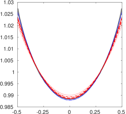
(a) Density, $\rho$

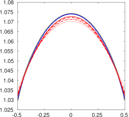
(b) Temperature, $\theta$

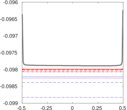
(c) Shear stress, $\sigma_{12}$

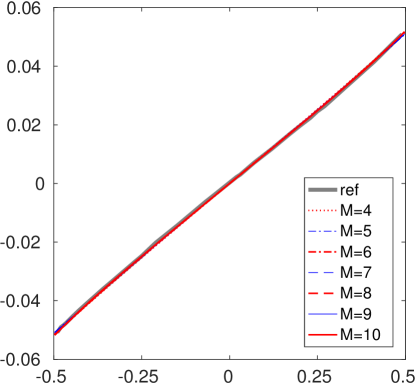
(d) Heat flux, $q_{1}$

Figure 1: Solution of the Couette flow for $\mathit{Kn}=0.1199$ on the uniform grid with $N=200$.

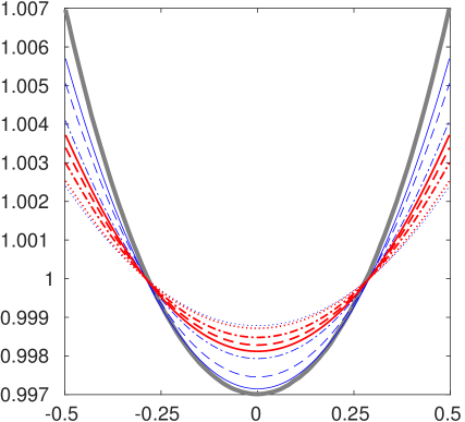
(a) Density, $\rho$

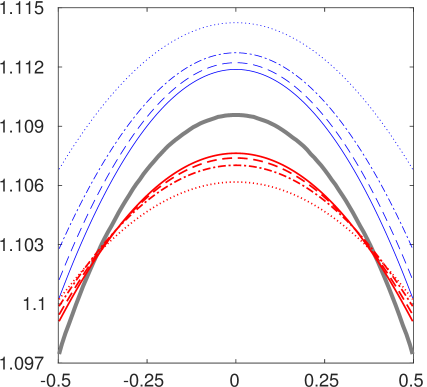
(b) Temperature, $\theta$

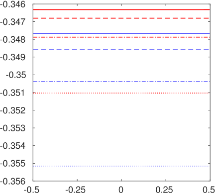
(c) Shear stress, $\sigma_{12}$

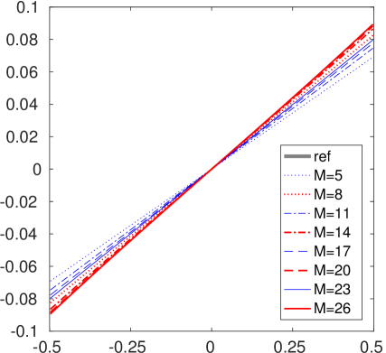
(d) Heat flux, $q_{1}$

Figure 2: Solution of the Couette flow for $\mathit{Kn}=1.199$ on the uniform grid with $N=200$.

Now we turn to investigate the efficiency and behavior of the NMLM solver proposed in previous sections. As we have done in [22], the NMLM solvers with various levels and order reduction strategies for the above Couette flow are performed on three uniform grids with $N=100$, $200$ and $400$, respectively. Due to the similar features of the NMLM solver with respect to $M$, only partial results are provided here.

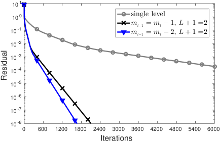
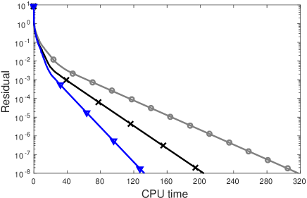
Figure 3: Convergence history of the NMLM solver for the Couette flow with $\mathit{Kn}=0.1199$ and $M=4$ on the uniform grid of $N=200$.

In the case of $\mathit{Kn}=0.1199$, the total number of iterations and the elapsed CPU seconds, spent by the steady-state computation of the solver, as well as the comparison to their counterparts of the single level solver, are listed in Table 1 for $M=4,5$ and in Table 2-3 for $M=10$, where $K$ and $T$ denote respectively the total number of iterations and the elapsed CPU seconds, and the corresponding quantities of the single level solver are denoted by $K_{s}$ and $T_{s}$. The convergence histories of the tests on the uniform grid with $N=200$ are plotted in Figure 3-5 for $M=4,5$ and $10$ respectively. It can be observed that the NMLM solver, in comparison to the single level solver, could accelerate the steady-state computation a lot for all tests. In more detail, the total number of the NMLM iterations, for the same $M$ and the same order reduction strategy, decreases as the total levels of the solver increases, which indicates the convergence rate is improved. Consequently, the elapsed CPU time is reduced as the total levels increases. For the NMLM solver with the same total levels, the convergence rate of the order reduction strategy $m_{\scriptscriptstyle l-1}=\lceil m_{\scriptscriptstyle l}/2\rceil$ is better than the strategy $m_{\scriptscriptstyle l-1}=m_{\scriptscriptstyle l}-2$, and the latter strategy is better than the strategy $m_{\scriptscriptstyle l-1}=m_{\scriptscriptstyle l}-1$. Apparently, the computational cost of each NMLM iteration for these three order reduction strategies is in the ascending sort, since smallest order is employed in each level of the lower-order moment model correction for the strategy $m_{\scriptscriptstyle l-1}=\lceil m_{\scriptscriptstyle l}/2\rceil$, while largest order is used in each level for the strategy $m_{\scriptscriptstyle l-1}=m_{\scriptscriptstyle l}-1$. Therefore, among these three order reduction strategies, the most efficient one becomes $m_{\scriptscriptstyle l-1}=\lceil m_{\scriptscriptstyle l}/2\rceil$, the second one is $m_{\scriptscriptstyle l-1}=m_{\scriptscriptstyle l}-2$, and the third one is $m_{\scriptscriptstyle l-1}=m_{\scriptscriptstyle l}-1$. Although more total levels can be applied for the strategies $m_{\scriptscriptstyle l-1}=m_{\scriptscriptstyle l}-2$ and $m_{\scriptscriptstyle l-1}=m_{\scriptscriptstyle l}-1$, they might still not be as efficient as the strategy $m_{\scriptscriptstyle l-1}=\lceil m_{\scriptscriptstyle l}/2\rceil$. Taking the tests for $M=10$ as an example, the $3$-level NMLM solver with the strategy $m_{\scriptscriptstyle l-1}=\lceil m_{\scriptscriptstyle l}/2\rceil$ is comparable with $5$-level NMLM solver with the strategy $m_{\scriptscriptstyle l-1}=m_{\scriptscriptstyle l}-2$, and both of them are more efficient than the $8$-level NMLM solver with the strategy $m_{\scriptscriptstyle l-1}=m_{\scriptscriptstyle l}-1$. At last, it can also be observed from Table 1-3 that the behavior of the NMLM solver with respect to the spatial grid number $N$ is just like the one of the single level solver, that is, the total number of NMLM iterations doubles and the elapsed CPU time quadruples, as $N$ doubles.

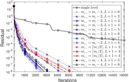
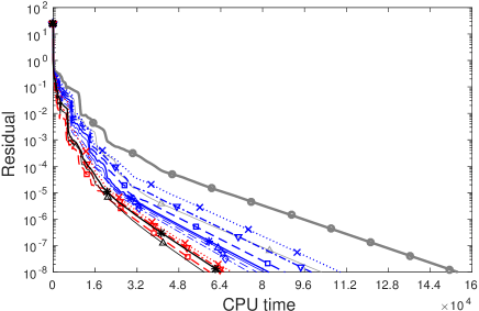
Figure 6: Convergence history of the NMLM solver for the Couette flow with $\mathit{Kn}=1.199$ and $M=23$ on the uniform grid of $N=200$.

As the Knudsen number increases to $\mathit{Kn}=1.199$, the moment model with a larger order needs to be considered. A partial numerical results can be found in Table 4 for $M=23$ and in Table 5 for $M=26$, respectively. The corresponding convergence histories on the uniform grid with $N=200$ are shown in Figure 6-7. Like the case of $\mathit{Kn}=0.1199$, it can be observed that the NMLM solver behaves similarly to the corresponding single level solver, as the grid number $N$ increases. The convergence rate of the NMLM solver with the same order reduction strategies is also improved as the total levels increases. The elapsed CPU time is consequently reduced except for the tests with $M=26$ and $m_{\scriptscriptstyle l-1}=m_{\scriptscriptstyle l}-2$, which is acceptable by noting that the convergence rate is improved a little, and the computational cost of lower-order moment model correction at each level could not be neglected, since the order sequence $26,24,22,\ldots$ is adopted. Moreover, oscillation of the residual at the beginning iterations and degeneracy of the convergence rate are observed for the single level solver, i.e., Heun’s method. This makes the residual oscillate more wildly and the convergence rate also be degenerated for the NMLM solver, especially for the solver with the strategy $m_{\scriptscriptstyle l-1}=\lceil m_{\scriptscriptstyle l}/2\rceil$, for which the convergence rate, in contrast to the case of $\mathit{Kn}=0.1199$, is now worse than the strategy $m_{\scriptscriptstyle l-1}=m_{\scriptscriptstyle l}-2$. Nevertheless, due to the great reduction of the computational cost at each NMLM iteration, the strategy $m_{\scriptscriptstyle l-1}=\lceil m_{\scriptscriptstyle l}/2\rceil$ is finally more efficient than the strategy $m_{\scriptscriptstyle l-1}=m_{\scriptscriptstyle l}-2$. As can be seen, more than $50\%$ of the total computational cost, compared with the single level solver, is saved by the $4$-level NMLM solver with the strategy $m_{\scriptscriptstyle l-1}=\lceil m_{\scriptscriptstyle l}/2\rceil$ in all tests for $M=23$ and $26$. In addition, to seek the balance between the convergence rate and the computational cost of each NMLM iteration, a new order reduction strategy, namely, $m_{\scriptscriptstyle l-1}=m_{\scriptscriptstyle l}-4$, is tested for $M=23$. As shown in Figure 6, it is found that the convergence rate of this strategy is better than the strategy $m_{\scriptscriptstyle l-1}=\lceil m_{\scriptscriptstyle l}/2\rceil$, and the elapsed CPU time of the $6$-level NMLM solver with the former strategy is a slightly less than the $4$-level NMLM solver with the latter strategy.

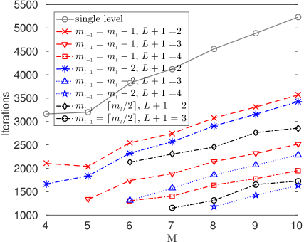
(a) $\mathit{Kn}=0.1199$

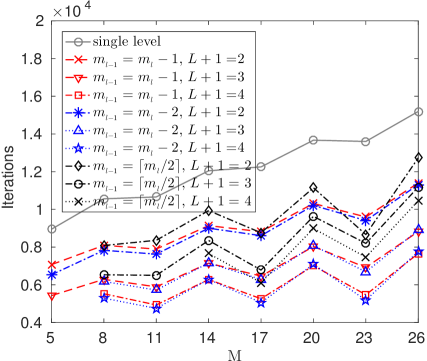
(b) $\mathit{Kn}=1.199$

Figure 8: Total number of iterations in terms of $M$ of the NMLM solver for the Couette flow on the uniform grid of $N=200$. The total number of iterations of the single level solver is rescaled by a factor of $6$.

Finally, the behavior of the total number of iterations with respect to the order of the moment model $M$ is investigated. The results are shown in Figure 8. It can be seen that in the case of $\mathit{Kn}=0.1199$, the total number of iterations increases almost linearly with the same ratio for all tests, as $M$ increases. While in the case of $\mathit{Kn}=1.199$, sawtooth polylines are observed for all tests. To be specific, the single level solver for odd $M$ performs much better than the solver for successor even $M$, and the growth rate of the total number of iterations with respect to odd or even $M$ is nearly the same. This shows better performance of Heun’s method than the SGS-Richardson iteration, in comparison to the results presented in [22]. For the multi-level NMLM solver, the different performance for odd or even $M$ becomes more obvious, especially for the strategy $m_{\scriptscriptstyle l-1}=\lceil m_{\scriptscriptstyle l}/2\rceil$. The underlying reason remains to be further studied. However, we can observe that the growth rate of the total number of iterations for the multi-level NMLM solver with respect to even $M$ is greater than the corresponding growth rate with respect to odd $M$, but still be almost not greater than the growth rate of the single level solver. As a result, the NMLM solver becomes more efficient for the moment model of odd $M$ than that of even $M$.

		$M=4$			$M=5$
			$m_{\scriptscriptstyle l-1}=m_{\scriptscriptstyle l}-1$	$m_{\scriptscriptstyle l-1}=m_{\scriptscriptstyle l}-2$		$m_{\scriptscriptstyle l-1}=m_{\scriptscriptstyle l}-1$		$m_{\scriptscriptstyle l-1}=m_{\scriptscriptstyle l}-2$
$L+1$		1	2	2	1	2	3	2
$N=100$	$K$	9484	1052	834	9595	1021	668	919
	$T$	74.711	51.155	33.326	124.430	78.879	62.440	60.092
	$K_{s}/K$	1.000	9.015	11.372	1.000	9.398	14.364	10.441
	$T_{s}/T$	1.000	1.460	2.242	1.000	1.577	1.993	2.071
$N=200$	$K$	18971	2104	1664	19191	2041	1335	1838
	$T$	317.736	204.048	132.755	504.057	315.070	248.836	238.401
	$K_{s}/K$	1.000	9.017	11.401	1.000	9.403	14.375	10.441
	$T_{s}/T$	1.000	1.557	2.393	1.000	1.600	2.026	2.114
$N=400$	$K$	37944	4208	3345	38382	4082	2668	3675
	$T$	1278.954	807.967	538.051	2028.431	1260.130	982.810	955.244
	$K_{s}/K$	1.000	9.017	11.343	1.000	9.403	14.386	10.444
	$T_{s}/T$	1.000	1.583	2.377	1.000	1.610	2.064	2.123

Table 1: Performance of the NMLM solver for the Couette flow with $\mathit{Kn}=0.1199$ and $M=4,5$.

		$m_{\scriptscriptstyle l-1}=m_{\scriptscriptstyle l}-1$
$L+1$		2	3	4	5	6	7	8
$N=100$	$K$	1784	1258	976	799	675	581	506
	$T$	883.677	781.440	704.394	623.006	553.480	492.187	442.410
	$K_{s}/K$	8.796	12.474	16.078	19.640	23.247	27.009	31.012
	$T_{s}/T$	1.336	1.511	1.676	1.895	2.133	2.399	2.669
$N=200$	$K$	3567	2514	1951	1595	1348	1159	1010
	$T$	3546.025	3164.404	2791.258	2521.665	2248.097	1988.022	1734.307
	$K_{s}/K$	8.798	12.483	16.085	19.675	23.280	27.077	31.071
	$T_{s}/T$	1.349	1.511	1.713	1.897	2.127	2.406	2.758
$N=400$	$K$	7133	5027	3900	3189	2693	2316	2017
	$T$	13688.115	12610.887	11097.524	10001.285	8973.447	7835.308	7006.392
	$K_{s}/K$	8.799	12.485	16.093	19.680	23.305	27.099	31.116
	$T_{s}/T$	1.332	1.446	1.643	1.824	2.032	2.328	2.603

Table 2: Performance of the NMLM solver for the Couette flow with $\mathit{Kn}=0.1199$ and $M=10$ (part I).

		$m_{\scriptscriptstyle l-1}=m_{\scriptscriptstyle l}-2$				$m_{\scriptscriptstyle l-1}=\lceil m_{\scriptscriptstyle l}/2\rceil$
$L+1$		2	3	4	5	2	3	1
$N=100$	$K$	1712	1144	818	560	1430	864	15692
	$T$	739.831	571.578	421.999	294.624	478.640	297.862	1180.762
	$K_{s}/K$	9.166	13.717	19.183	28.021	10.973	18.162	1.000
	$T_{s}/T$	1.596	2.066	2.798	4.008	2.467	3.964	1.000
$N=200$	$K$	3423	2287	1634	1118	2859	1728	31382
	$T$	2940.028	2250.739	1694.924	1165.652	1923.646	1155.322	4782.708
	$K_{s}/K$	9.168	13.722	19.206	28.070	10.977	18.161	1.000
	$T_{s}/T$	1.627	2.125	2.822	4.103	2.486	4.140	1.000
$N=400$	$K$	6845	4572	3265	2234	5716	3454	62761
	$T$	11978.715	8947.557	6792.666	4643.324	7329.159	4726.841	18238.107
	$K_{s}/K$	9.169	13.727	19.222	28.094	10.980	18.171	1.000
	$T_{s}/T$	1.523	2.038	2.685	3.928	2.488	3.858	1.000

Table 3: Performance of the NMLM solver for the Couette flow with $\mathit{Kn}=0.1199$ and $M=10$ (part II).

		$m_{\scriptscriptstyle l-1}=m_{\scriptscriptstyle l}-2$					$m_{\scriptscriptstyle l-1}=\lceil m_{\scriptscriptstyle l}/2\rceil$
$L+1$		4	5	6	7	8	2	3	4
$N=100$	$K$	2580	2194	2033	1910	1802	4198	4111	3737
	$T$	21771.636	20636.803	20038.953	18945.630	18761.918	16608.830	16448.863	14880.760
	$K_{s}/K$	15.820	18.603	20.076	21.369	22.650	9.722	9.928	10.922
	$T_{s}/T$	1.776	1.874	1.929	2.041	2.061	2.328	2.351	2.598
$N=200$	$K$	5188	4427	4096	3853	3644	8665	8195	7465
	$T$	88518.030	82354.633	80539.022	77774.608	74883.559	68274.318	65399.218	59797.985
	$K_{s}/K$	15.733	18.437	19.927	21.184	22.399	9.420	9.960	10.934
	$T_{s}/T$	1.746	1.877	1.919	1.987	2.064	2.264	2.363	2.584
$N=400$	$K$	10396	8875	8203	7715	7298	17519	16362	14896
	$T$	351768.755	332364.873	323203.956	313285.091	300010.067	274114.156	258269.847	236863.512
	$K_{s}/K$	15.702	18.393	19.900	21.159	22.368	9.318	9.977	10.959
	$T_{s}/T$	1.743	1.845	1.897	1.957	2.044	2.237	2.374	2.588

Table 4: Performance of the NMLM solver for the Couette flow with $\mathit{Kn}=1.199$ and $M=23$.

		$m_{\scriptscriptstyle l-1}=m_{\scriptscriptstyle l}-2$					$m_{\scriptscriptstyle l-1}=\lceil m_{\scriptscriptstyle l}/2\rceil$
$L+1$		4	5	6	7	8	2	3	4	5
$N=100$	$K$	3882	3567	3372	3239	3143	6368	5594	5234	5042
	$T$	48452.216	49497.714	49879.413	50491.512	50094.156	36028.855	31647.628	29804.057	28720.545
	$K_{s}/K$	11.784	12.825	13.566	14.123	14.555	7.184	8.178	8.740	9.073
	$T_{s}/T$	1.267	1.240	1.231	1.216	1.225	1.704	1.940	2.060	2.137
$N=200$	$K$	7768	7143	6753	6488	6295	12731	11183	10457	10064
	$T$	193489.560	199169.100	199861.340	202753.586	199230.828	142907.221	126167.456	118536.002	114107.992
	$K_{s}/K$	11.736	12.763	13.500	14.051	14.482	7.161	8.152	8.718	9.058
	$T_{s}/T$	1.268	1.232	1.227	1.210	1.231	1.717	1.944	2.069	2.150
$N=400$	$K$	15538	14293	13516	12987	12600	25447	22360	20902	20107
	$T$	772099.850	792816.382	801340.202	805215.081	797777.655	573505.900	506611.853	473278.177	458730.507
	$K_{s}/K$	11.735	12.757	13.491	14.040	14.472	7.166	8.155	8.724	9.069
	$T_{s}/T$	1.296	1.262	1.248	1.242	1.254	1.744	1.975	2.114	2.181

Table 5: Performance of the NMLM solver for the Couette flow with $\mathit{Kn}=1.199$ and $M=26$.

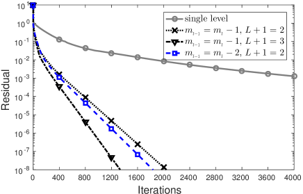
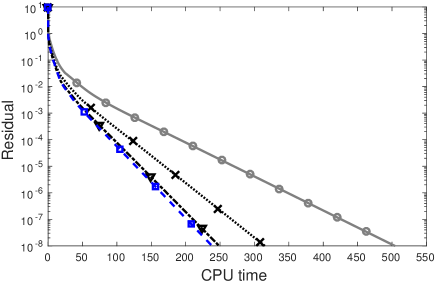
Figure 4: Convergence history of the NMLM solver for the Couette flow with $\mathit{Kn}=0.1199$ and $M=5$ on the uniform grid of $N=200$.

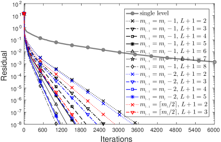
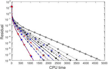
Figure 5: Convergence history of the NMLM solver for the Couette flow with $\mathit{Kn}=0.1199$ and $M=10$ on the uniform grid of $N=200$.

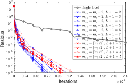
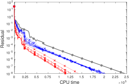
Figure 7: Convergence history of the NMLM solver for the Couette flow with $\mathit{Kn}=1.199$ and $M=26$ on the uniform grid of $N=200$.

4.2 The force driven Poiseuille flow

The second example is the force driven Poiseuille flow which has been investigated in the literature, see e.g. [8, 34, 35]. The gas lies between two infinite parallel plates which are stationary and have the same temperature of $\theta^{W}=1$. It is driven by an external constant force and has a steady state as time goes. In our simulation, the distance of the two plates is assumed to be $L_{D}=1$, and the acceleration due to the external force is set to be $\boldsymbol{F}=(0,0.2555,0)^{T}$. The collision frequency for the variable hard sphere model, that is,

$$\nu=\sqrt{\frac{2}{\pi}}\frac{(5-2w)(7-2w)\Pr}{15\mathit{Kn}}\rho\theta^{1-w},$$ (28)

with the viscosity index $w=0.5$ and the Knudsen number $\mathit{Kn}=0.1$ is adopted.

With these settings, the steady-state solutions for density $\rho$, temperature $\theta$, normal stress $\sigma_{11}$ and heat flux $q_{2}$, obtained by the NMLM solver on the uniform grid with $N=200$, are shown in Figure 9, which coincide well with the steady-state solutions presented in [21], where the first-order spatial discretization with $N=2048$ is employed.

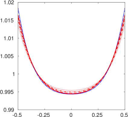
(a) Density, $\rho$

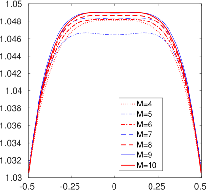
(b) Temperature, $\theta$

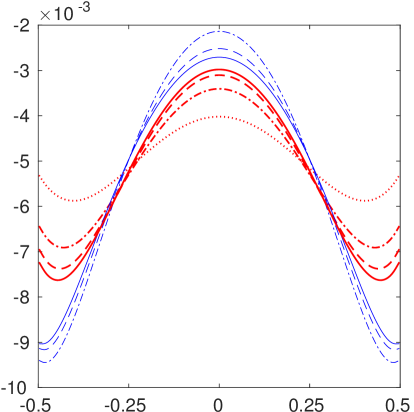
(c) Normal stress, $\sigma_{11}$

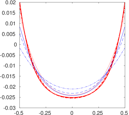
(d) Heat flux, $q_{2}$

Figure 9: Solution of the force driven Poiseuille flow on the uniform grid with $N=200$.

For the efficiency and behavior of the proposed NMLM solver, the tests with various levels and order reduction strategies are performed on three uniform grids with $N=100$, $200$ and $400$ for the moment model with the order from $M=4$ to $10$. As the Couette flow, only partial numerical results are presented here. Specifically, the total number of iterations and the elapsed CPU seconds are given in Table 6 for $M=4,5$ and in Table 7-8 for $M=10$ respectively. The corresponding convergence histories of the tests on the uniform grid with $N=200$ are displayed in Figure 10-12. The total number of iterations in terms of $M$ is presented in Figure 13LABEL:sub@fig:poiseuille-fourier:poiseuille. All results show similar features as the tests of the Couette flow in the case of $\mathit{Kn}=0.1199$, which indicates the effectiveness of the NMLM solver in accelerating the steady-state computation.

		$M=4$			$M=5$
			$m_{\scriptscriptstyle l-1}=m_{\scriptscriptstyle l}-1$	$m_{\scriptscriptstyle l-1}=m_{\scriptscriptstyle l}-2$		$m_{\scriptscriptstyle l-1}=m_{\scriptscriptstyle l}-1$		$m_{\scriptscriptstyle l-1}=m_{\scriptscriptstyle l}-2$
$L+1$		1	2	2	1	2	3	2
$N=100$	$K$	15676	1632	1388	18621	2022	1340	1788
	$T$	157.124	87.112	60.254	268.329	178.323	140.127	130.205
	$K_{s}/K$	1.000	9.605	11.294	1.000	9.209	13.896	10.414
	$T_{s}/T$	1.000	1.804	2.608	1.000	1.505	1.915	2.061
$N=200$	$K$	31349	3263	2775	37251	4044	2679	3576
	$T$	566.855	345.652	239.170	1068.763	704.765	559.148	517.321
	$K_{s}/K$	1.000	9.607	11.297	1.000	9.211	13.905	10.417
	$T_{s}/T$	1.000	1.640	2.370	1.000	1.516	1.911	2.066
$N=400$	$K$	62694	6524	5590	74509	8088	5358	7152
	$T$	2280.702	1382.533	971.918	4291.040	2818.351	2232.552	2070.655
	$K_{s}/K$	1.000	9.610	11.215	1.000	9.212	13.906	10.418
	$T_{s}/T$	1.000	1.650	2.347	1.000	1.523	1.922	2.072

Table 6: Performance of the NMLM solver for the Poiseuille flow with $M=4,5$.

		$m_{\scriptscriptstyle l-1}=m_{\scriptscriptstyle l}-1$
$L+1$		2	3	4	5	6	7	8
$N=100$	$K$	3312	2333	1808	1477	1244	1067	921
	$T$	1849.890	1662.403	1491.818	1353.205	1145.176	1043.163	905.261
	$K_{s}/K$	8.803	12.496	16.125	19.739	23.436	27.323	31.655
	$T_{s}/T$	1.388	1.545	1.721	1.898	2.243	2.462	2.837
$N=200$	$K$	6625	4667	3616	2953	2487	2133	1840
	$T$	7498.892	6641.554	5983.719	5250.433	4644.889	4111.988	3637.646
	$K_{s}/K$	8.804	12.498	16.131	19.752	23.454	27.346	31.701
	$T_{s}/T$	1.304	1.472	1.634	1.862	2.105	2.378	2.688
$N=400$	$K$	13251	9333	7232	5905	4973	4264	3677
	$T$	29539.018	26645.046	23642.063	21103.438	18830.564	16646.179	14537.716
	$K_{s}/K$	8.804	12.501	16.132	19.757	23.460	27.361	31.729
	$T_{s}/T$	1.301	1.443	1.626	1.822	2.042	2.309	2.644

Table 7: Performance of the NMLM solver for the Poiseuille flow with $M=10$ (part I).

		$m_{\scriptscriptstyle l-1}=m_{\scriptscriptstyle l}-2$				$m_{\scriptscriptstyle l-1}=\lceil m_{\scriptscriptstyle l}/2\rceil$
$L+1$		2	3	4	5	2	3	1
$N=100$	$K$	3179	2123	1517	1059	2643	1560	29154
	$T$	1561.039	1201.458	888.561	638.520	989.148	613.051	2568.151
	$K_{s}/K$	9.171	13.732	19.218	27.530	11.031	18.688	1.000
	$T_{s}/T$	1.645	2.138	2.890	4.022	2.596	4.189	1.000
$N=200$	$K$	6359	4246	3034	2116	5287	3120	58329
	$T$	6339.990	4754.203	3596.238	2505.962	3942.316	2424.629	9778.709
	$K_{s}/K$	9.173	13.737	19.225	27.566	11.033	18.695	1.000
	$T_{s}/T$	1.542	2.057	2.719	3.902	2.480	4.033	1.000
$N=400$	$K$	12718	8491	6067	4231	10574	6239	116668
	$T$	25255.174	18999.092	14340.679	10061.378	15946.033	9624.905	38442.738
	$K_{s}/K$	9.173	13.740	19.230	27.575	11.033	18.700	1.000
	$T_{s}/T$	1.522	2.023	2.681	3.821	2.411	3.994	1.000

Table 8: Performance of the NMLM solver for the Poiseuille flow with $M=10$ (part II).

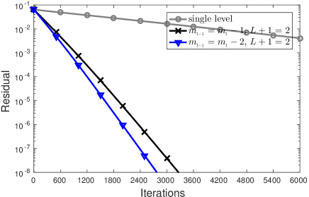
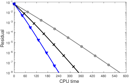
Figure 10: Convergence history of the NMLM solver for the Poiseuille flow with $M=4$ on the uniform grid of $N=200$.

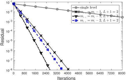
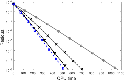
Figure 11: Convergence history of the NMLM solver for the Poiseuille flow with $M=5$ on the uniform grid of $N=200$.

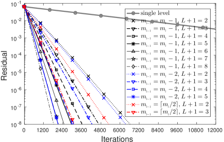
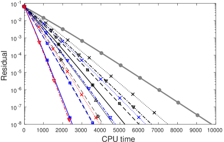
Figure 12: Convergence history of the NMLM solver for the Poiseuille flow with $M=10$ on the uniform grid of $N=200$.

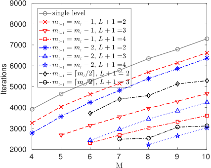
(a) Poiseuille flow

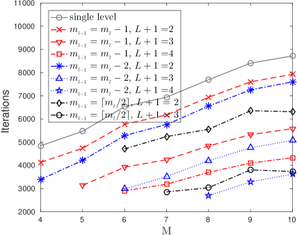
(b) Fourier flow

Figure 13: Total number of iterations in terms of $M$ of the NMLM solver on the uniform grid of $N=200$. The total number of iterations of the single level solver is rescaled by a factor of $8$.

4.3 The Fourier flow

The last benchmark test is the Fourier flow which also investigates the motion of the gas between two infinite parallel plates with a distance of $L_{D}=1$. In contrast to the previous examples, both plates are stationary, while their temperatures are different. The gas is driven by the difference of temperatures between the two plates, and could reach a steady state in the absence of external force, that is, $\boldsymbol{F}\equiv 0$. To reproduce the results in [9, 32], the gas of helium with the viscosity index $w=0.657$ and the Knudsen number $\mathit{Kn}=0.1044$ for the collision frequency (28) is considered. The temperature on the left plate and the right plate are set to be 0.2894 and 1.0769 respectively. Numerical solutions for density $\rho$ and temperature $\theta$, obtained by the NMLM solver on the uniform grid with $N=200$, are shown in Figure 14. The solutions obtained by the DSMC (Direct Simulation of Monte Carlo) method [32] are provided as a reference. It can be observed that the solutions of the moment model converge and match the DSMC solution well as the order $M$ increases.

As for the performance of the NMLM solver, the tests with various levels and order reduction strategies are also performed on three uniform grids with $N=100$, $200$ and $400$ for the moment model with the order from $M=4$ to $10$. Due to the same reason, only partial numerical results are presented here. That is, the total number of iterations and the elapsed CPU seconds for $M=10$ are given in Table 9-10. The corresponding convergence histories of the tests on the uniform grid with $N=200$ are displayed in Figure 15. And the total number of iterations in terms of $M$ is plotted in Figure 13LABEL:sub@fig:poiseuille-fourier:fourier. Again, all results show similar features as the tests of the Couette flow in the case of $\mathit{Kn}=0.1199$ and the tests of the Poiseuille flow. Therefore, the proposed NMLM solver is indeed able to accelerate the steady-state computation significantly.

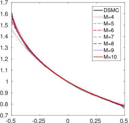
(a) Density, $\rho$

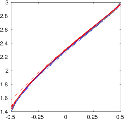
(b) Temperature, $\theta$

Figure 14: Solution of the Fourier flow on the uniform grid with $N=200$.

		$m_{\scriptscriptstyle l-1}=m_{\scriptscriptstyle l}-1$
$L+1$		2	3	4	5	6	7	8
$N=100$	$K$	3965	2794	2167	1771	1493	1282	1109
	$T$	1860.858	1694.069	1523.898	1363.943	1209.693	1075.778	930.812
	$K_{s}/K$	8.799	12.486	16.099	19.699	23.367	27.213	31.458
	$T_{s}/T$	1.592	1.749	1.944	2.172	2.449	2.754	3.183
$N=200$	$K$	7928	5585	4331	3539	2983	2560	2214
	$T$	7415.489	6720.777	6035.377	5384.300	4840.328	4236.370	3750.768
	$K_{s}/K$	8.799	12.490	16.106	19.711	23.385	27.248	31.507
	$T_{s}/T$	1.593	1.758	1.958	2.194	2.441	2.789	3.150
$N=400$	$K$	15851	11167	8659	7074	5962	5116	4424
	$T$	29739.900	26760.605	24140.459	21534.845	19151.365	17020.835	14997.699
	$K_{s}/K$	8.800	12.491	16.109	19.718	23.396	27.265	31.530
	$T_{s}/T$	1.527	1.697	1.881	2.108	2.371	2.667	3.027

Table 9: Performance of the NMLM solver for the Fourier flow with $M=10$ (part I).

		$m_{\scriptscriptstyle l-1}=m_{\scriptscriptstyle l}-2$				$m_{\scriptscriptstyle l-1}=\lceil m_{\scriptscriptstyle l}/2\rceil$
$L+1$		2	3	4	5	2	3	1
$N=100$	$K$	3803	2540	1814	1252	3159	1870	34887
	$T$	1579.625	1213.639	907.115	631.572	975.638	603.752	2962.720
	$K_{s}/K$	9.174	13.735	19.232	27.865	11.044	18.656	1.000
	$T_{s}/T$	1.876	2.441	3.266	4.691	3.037	4.907	1.000
$N=200$	$K$	7603	5076	3624	2502	6314	3735	69756
	$T$	6361.864	4843.804	3627.384	2553.007	3926.485	2419.668	11815.652
	$K_{s}/K$	9.175	13.742	19.248	27.880	11.048	18.676	1.000
	$T_{s}/T$	1.857	2.439	3.257	4.628	3.009	4.883	1.000
$N=400$	$K$	15203	10149	7244	5001	12622	7465	139487
	$T$	25136.041	19347.345	14581.706	10236.093	15873.863	9702.212	45400.647
	$K_{s}/K$	9.175	13.744	19.256	27.892	11.051	18.685	1.000
	$T_{s}/T$	1.806	2.347	3.114	4.435	2.860	4.679	1.000

Table 10: Performance of the NMLM solver for the Fourier flow with $M=10$ (part II).

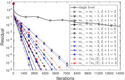
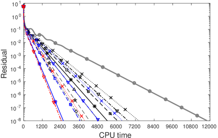
Figure 15: Convergence history of the NMLM solver for the Fourier flow with $M=10$ on the uniform grid of $N=200$.

5 Concluding remarks

A steady-state solver for microflows with high-order moment model was successfully proposed in this paper, which significantly improved the efficiency of the one in [22] from the following approaches:

• Linear reconstruction is adopted for high-resolution spatial discretization, so that remarkable reduction for degrees of freedom in spatial space is obtained without loss of accuracy.

• A relaxation parameter is introduced in the correction step to enhance the stability of the solver such that more levels can be applied in the solver.

• The computation of the correction step is also simplified a lot in comparison to the way used in [22].

• Heun’s method is taken as the smoother in each level to further improve the robustness of the NMLM solver in the situation when many levels are involved.

The performance of the new NMLM solver is numerically investigated by three benchmark problems in microflows. Various order reduction strategies for the choice of the order sequence of the NMLM solver have been tested. For each order reduction strategy, the convergence rate of the resulting NMLM solver is improved as the total levels increases. Among these order reduction strategies, it is shown that the most efficient strategy is $m_{\scriptscriptstyle l-1}=\lceil m_{\scriptscriptstyle l}/2\rceil$, and the second strategy is $m_{\scriptscriptstyle l-1}=m_{\scriptscriptstyle l}-2$. In summary, it is demonstrated that the new NMLM solver can further improve the efficiency of steady-state computations even for the moment model with a relatively small order, such as $M=4$ and $5$. As a result, the idea of using the lower-order moment model correction is very promising to accelerate the steady-state simulation, and may also be valuable for problems described by other hierarchical models.

Additionally, the NMLM solver behaves similarly to the single level solver, as the order $M$ or the spatial grid number $N$ increases. Research works on combination of the lower-order moment model correction with the spatial coarse grid correction are ongoing.

References

- [1] P. L. Bhatnagar, E. P. Gross, and M. Krook. A model for collision processes in gases. I. small amplitude processes in charged and neutral one-component systems. Phys. Rev., 94(3):511–525, 1954.
- [2] A. Brandt and O. E. Livne. Multigrid Techniques: 1984 Guide with Applications to Fluid Dynamics. Classics in Applied Mathematics. SIAM, revised edition, 2011.
- [3] Z. Cai, Y. Fan, and R. Li. Globally hyperbolic regularization of Grad’s moment system. Comm. Pure Appl. Math., 67(3):464–518, 2014.
- [4] Z. Cai, Y. Fan, and R. Li. On hyperbolicity of 13-moment system. Kinet. Relat. Mod., 7(3):415–432, 2014.
- [5] Z. Cai, Y. Fan, and R. Li. A framework on moment model reduction for kinetic equation. SIAM J. Appl. Math., 75(5):2001–2023, 2015.
- [6] Z. Cai, Y. Fan, R. Li, and Z. Qiao. Dimension-reduced hyperbolic moment method for the Boltzmann equation with BGK-type collision. Commun. Comput. Phys., 15(5):1368–1406, 2014.
- [7] Z. Cai and R. Li. Numerical regularized moment method of arbitrary order for Boltzmann-BGK equation. SIAM J. Sci. Comput., 32(5):2875–2907, 2010.
- [8] Z. Cai, R. Li, and Z. Qiao. NR simulation of microflows with Shakhov model. SIAM J. Sci. Comput., 34(1):A339–A369, 2012.
- [9] Z. Cai, R. Li, and Z. Qiao. Globally hyperbolic regularized moment method with applications to microflow simulation. Computers and Fluids, 81:95–109, 2013.
- [10] Z. Cai, R. Li, and Y. Wang. An efficient NR method for Boltzmann-BGK equation. J. Sci. Comput., 50(1):103–119, 2012.
- [11] S. Chapman and T. G. Cowling. The Mathematical Theory of Non-uniform Gases, Third Edition. Cambridge University Press, 1990.
- [12] Y. Di, Y. Fan, R. Li, and L. Zheng. Linear stability of hyperbolic moment models for Boltzmann equation. Numerical Mathematics: Theory, Method and Application, 10(2):255–277, 2017.
- [13] K. J. Fidkowski, T. A. Oliver, J. Lu, and D. L. Darmofal. -Multigrid solution of high-order discontinuous Galerkin discretizations of the compressible Navier-Stokes equations. J. Comput. Phys., 207(1):92–113, Jul 2005.
- [14] I. M. Gamba, J. R. Haack, C. D. Hauck, and J. Hu. A fast spectral method for the Boltzmann collision operator with general collision kernels. SIAM Journal on Scientific Computing, 39(14):B658–B674, 2017.
- [15] H. Grad. On the kinetic theory of rarefied gases. Comm. Pure Appl. Math., 2(4):331–407, 1949.
- [16] H. Grad. The profile of a steady plane shock wave. Comm. Pure Appl. Math., 5(3):257–300, 1952.
- [17] W. Hackbusch. Multi-Grid Methods and Applications. Springer-Verlag, Berlin, 1985. second printing 2003.
- [18] S. Harris. An Introduction to the Theory of the Boltzmann Equation. Dover Publications, New York, 2004.
- [19] B. T. Helenbrook and H. L. Atkins. Solving discontinuous Galerkin formulations of Poisson’s equation using geometric and multigrid. AIAA Journal, 46(4):894–902, Apr 2008.
- [20] L. H. Holway. New statistical models for kinetic theory: Methods of construction. Phys. Fluids, 9(1):1658–1673, 1966.
- [21] Z. Hu and R. Li. A nonlinear multigrid steady-state solver for 1D microflow. Computers and Fluids, 103:193–203, 2014.
- [22] Z. Hu, R. Li, and Z. Qiao. Acceleration for microflow simulations of high-order moment models by using lower-order model correction. J. Comput. Phys., 327:225–244, DEC 2016.
- [23] Z. Hu, R. Li, and Z. Qiao. Extended hydrodynamic models and multigrid solver of a silicon diode simulation. Commun. Comput. Phys., 20(3):551–582, Sep 2016.
- [24] C. D. Levermore. Moment closure hierarchies for kinetic theories. J. Stat. Phys., 83(5–6):1021–1065, 1996.
- [25] Y. Maday and R. Muñoz. Spectral element multigrid. II. Theoretical justification. J. Sci. Comput., 3(4):323–353, 1988.
- [26] J. McDonald and M. Torrilhon. Affordable robust moment closures for CFD based on the maximum-entropy hierarchy. J. Comput. Phys., 251:500–523, 2013.
- [27] L. Mieussens and H. Struchtrup. Numerical comparison of Bhatnagar-Gross-Krook models with proper Prandtl number. Phys. Fluids, 16(8):2797–2813, 2004.
- [28] E. M. Rønquist and A. T. Patera. Spectral element multigrid. I. Formulation and numerical results. J. Sci. Comput., 2(4):389–406, 1987.
- [29] E. M. Shakhov. Generalization of the Krook kinetic relaxation equation. Fluid Dyn., 3(5):95–96, 1968.
- [30] H. Struchtrup. Macroscopic Transport Equations for Rarefied Gas Flows: Approximation Methods in Kinetic Theory. Springer, 2005.
- [31] H. Struchtrup and M. Torrilhon. Regularized 13 moment equations for hard sphere molecules: I. linear bulk equations. Phys. Fluids, 25(5):052001, 2013.
- [32] D. C. Wadsworth. Slip effects in a confined rarefied gas. I: Temperature slip. Phys. Fluids, 5(7):1831–1839, 1993.
- [33] Y. Wang and Z. Cai. Approximation of the Boltzmann collision operator based on Hermite spectral method. arXiv:1803.11191, 2018.
- [34] K. Xu, H. Liu, and J. Jiang. Multiple-temperature model for continuum and near continuum flows. Phys. Fluids, 19(1):016101, 2007.
- [35] Y. Zheng, A. L. Garcia, and B. J. Alder. Comparison of kinetic theory and hydrodynamics for Poiseuille flow. J. Stat. Phys., 109(3–4):495–505, 2002.