Stochastic subgrid-scale parameterization for one-dimensional shallow water dynamics using stochastic mode reduction

Abstract

We address the question of parameterizing the subgrid scales in simulations of geophysical flows by applying stochastic mode reduction to the one-dimensional stochastically forced shallow water equations. The problem is formulated in physical space by defining resolved variables as local spatial averages over finite-volume cells and unresolved variables as corresponding residuals. Based on the assumption of a time-scale separation between the slow spatial averages and the fast residuals, the stochastic mode reduction procedure is used to obtain a low-resolution model for the spatial averages alone with local stochastic subgrid-scale parameterization coupling each resolved variable only to a few neighboring cells. The closure improves the results of the low-resolution model and outperforms two purely empirical stochastic parameterizations. It is shown that the largest benefit is in the representation of the energy spectrum. By adjusting only a single coefficient (the strength of the noise) we observe that there is a potential for improving the performance of the parameterization, if additional tuning of the coefficients is performed. In addition, the scale-awareness of the parameterizations is studied.

1 Introduction

Atmospheric processes encompass a large spectrum of spatial and temporal scales. These range from several millimeters and seconds for boundary layer turbulence up to $10^{7}$ meters and several weeks (and even longer) for planetary wave dynamics. Due to limited computer resources numerical atmospheric models cannot describe all these processes on all scales simultaneously. However, the different scales are interacting in a complex manner and this leads to the challenging problem of parameterizing the effect of the unresolved subgrid-scale (SGS) processes onto the resolved ones. Examples include the parameterization of synoptic and mesoscale eddies in planetary scale atmospheric models (e.g. [47, 60]), momentum and temperature fluxes in the atmospheric boundary layer [54] or SGS Reynold stresses in large eddy simulations (e.g. [49]).

In this context, stochastic elements have become increasingly popular. Stochastic parameterizations can reduce a systematic model error, represent uncertainty in predictions, or trigger regime transitions (e.g. [42, 6]). Typically some ad-hoc SGS model is assumed and the corresponding coefficients are optimized (tuned) so as to obtain the best possible agreement, in some sense, with observations or high-resolution simulations. Examples in comprehensive climate and weather models are stochastically perturbed parameterization tendencies [7, 43] or stochastic kinetic energy backscatter [52, 5]. Empirical Ornstein-Uhlenbeck (OU) processes have been used in some studies of low-frequency and large-scale atmospheric variability (e.g. [61, 41, 46]), which can be extended to include quadratic nonlinearities as well as a time correlated stochastic forcing [32, 30].

With regard to SGS parameterizations in climate models issues can arise from the fact that they are typically tuned to optimally represent the statistics of the present-day climate. If climate changes due to some external forcing, it is not guaranteed that the tuned parameters are still optimal. The fluctuation-dissipation theorem might be able to provide corrections [3, 48] in some cases, but such an approach relies on the perturbations being sufficiently weak. Moreover, there is a need for scale-aware parameterizations in atmosphere modeling, as model resolution increases continuously and mesh refinement techniques become widely used. In addition, the consistency between particular SGS parameterizations and the numerical discretization becomes important.

These considerations motivate the development of other approaches where the SGS parameterization is derived from first principles, if possible without any empirical parameter optimization. The direct interaction approximation (DIA) introduced by [31] allowed to successfully apply statistical dynamical closure theory in relevant geophysical flows [17, 20, 18]. In the presence of time scale separation, the asymptotic method of averaging has been applied [23, 25, 4, 40]. This method requires an estimation of the invariant measure of the fast scales conditioned on the slow scales, which might limit its applicability when going to high-dimensional systems. Another promising approach, without any empirical component, is based on the maximum entropy principle [56, 58, 57]. Recently, [63, 64] have introduced a new method originating from response theory. This method relies on a weak coupling between resolved and unresolved scales and it has been applied to simple and more complex settings [62, 11, 59].

The DIA parameterization has been successfully applied to barotropic [17] and primitive equations model [18], it has been extended to include the effects of mean flow and topography [20]. The DIA closure is derived in spectral space by considering the evolution of second-order cumulant and response function. Next, the nonlinear damping rate and nonlinear noise are introduced. This results in a globally coupled SGS model in spectral space. However, techniques have been proposed to simplify the equations and obtain locally coupled models reproducing the spectra from direct numerical simulations [17, 18].

Another nearly self-consistent possibility that exploits a separation of time scales between resolved and unresolved scales is the stochastic mode reduction (SMR) procedure proposed by [37, 35, 38]. The SMR is a homogenization technique for multiscale systems ([27, 26, 33, 44] and a recent overview [45] and references therein) and it is supplemented by an empirical step, where the fast SGS self-interactions in the evolution equation for the unresolved modes are replaced by an OU process. Following this step, an analytical derivation of a stochastic parameterization for the fast modes is possible, rigorously valid in the limit of infinite time scale separation.

So far the SMR procedure has already been applied to balanced models, such as barotropic [16] and quasi-geostrophic [15] dynamics. The separation between resolved and unresolved scales has been performed by using empirical orthogonal functions (EOFs). However, EOFs are sometimes not able to guarantee a sufficient separation of the underlying time scales (e.g. Figure 3 in [15]). The SMR carried out in spectral space [16, 15] is quite similar to the DIA closure approach. In particular, the main goal of both techniques is to represent the subgrid processes by a nonlinear damping and a state-dependent noise and both techniques have been utilized successfully in geophysical flows.

In applications of the SMR to spectral space the resulting reduced model is globally coupled with linear, quadratic and even cubic terms. This hampers the applicability of the technique when high-dimensional systems with large number of resolved modes are considered. However, the latter problem can be avoided by applying the SMR in physical space to a finite-volume discretization of the equations. Such discretization does not per se include global coupling as in spectral discretizations, since grid cells interact directly only with a small number of neighbors. Finite-volume schemes are traditionally applied in ocean models (e.g. [22]), regional atmospheric modeling (e.g. [53]) and recently even for global atmospheric models as well [50, 39, 51]. In the examples above complex boundaries, such as continental boundaries in ocean modeling or non-periodic lateral boundaries in regional area atmospheric modeling, necessitate the use of discretizations and SGS parameterizations formulated in physical space. This motivated [12, 13] to consider a local approach where the resolved variables are defined by local spatial averages and the SGS flow by deviations from these averages, a configuration typically encountered in large-eddy turbulence parameterization (e.g. [49]). The local definition leads to a local SGS parameterization, coupling only near neighbors, as shown for the Burgers equation [12, 13]. The efficient local stochastic SGS parameterization allows to consider large numbers of resolved scales. In addition, the clear gap of spatial scales between the resolved and unresolved variables enables a more pronounced time-scale separation.

Obviously Burgers equation represents a highly idealized prototype model for testing various statistical and closure methods and it is necessary to verify the applicability of the SMR for local spatial averages for more realistic fluid-dynamical models. One step in this direction is performed in this work by applying the approach to a stochastically forced one-dimensional shallow water layer (1DSW). It incorporates at least two issues of relevance in the general context. First, in contrast to the Burgers equation the 1DSW allows for gravity waves. Secondly, if formulated in flux form, the shallow-water flow dynamical equations entail non-polynomial nonlinearities. This problem is of broader relevance, since such highly nonlinear terms appear in the general compressible fluid flow equations as well, in the pressure-gradient acceleration.

The work presented here can be summarized as follows. Based on a high-resolution finite-volume discretization of the shallow-water equations we use in Sec. 2 local spatial averages to define coarse and slow (resolved) variables and, via corresponding residuals, fine and fast (unresolved) variables. The assumed time-scale separation is verified numerically. The SMR theory for obtaining an SGS parameterization of the unresolved modes is then introduced and applied to the specific problem. In Sec. 3 we discuss the practical implementation, and also introduce, for comparison, two purely empirical approaches. Results from model simulations with the various SGS parameterizations are then compared in Sec. 4. Here we also investigate the scale awareness of the approaches, i.e. their ability to be applied at different resolutions without any re-tuning. Conclusions are finally drawn in Sec. 5.

2 Method

2.1 Shallow water model

We consider a stochastically forced one dimensional shallow water layer with periodic boundaries, using as variables the height of the fluid $h$ and the momentum $hu$, where $u$ is the velocity. The governing equations with plane topography (e.g. [55]) read in flux form

$$\partial_{t}\left(\begin{array}[]{c}h\\ hu\end{array}\right)=-\partial_{x}\left(\begin{array}[]{c}hu-\nu\partial_{x}h\\ \frac{(hu)^{2}}{h}+\frac{g}{2}h^{2}-\nu\partial_{x}hu\end{array}\right)+\boldsymbol{\varrho},$$ (5)

with a large-scale stochastic forcing $\boldsymbol{\varrho}$ (see Sec. 3) and a mass weighted diffusion with the constant parameter $\nu$.

For a high-resolution spatial discretization the domain of length $L$ is divided into $N$ fine intervals $\Delta x=L/N$ , labelled by a small index $i\in\{0,1,...,N-1\}$. With this the equations in (5) can be discretized by a symmetric finite-volume scheme

$$\frac{d}{dt}\left(\begin{array}[]{c}h_{i}\\ hu_{i}\end{array}\right)=-\frac{1}{\Delta x}\left(\textbf{F}_{i+\frac{1}{2}}-\textbf{F}_{i-\frac{1}{2}}\right)+\boldsymbol{\varrho}_{i}\;,$$ (8)

with the discrete forcing $\boldsymbol{\varrho}_{i}$ and the flux at the boundary given by

$$\textbf{F}_{i+\frac{1}{2}}=\frac{1}{2}\left(\begin{array}[]{c}\displaystyle{(hu)_{i+1}+(hu)_{i}-2\nu\frac{h_{i+1}-h_{i}}{\Delta x}}\\ \displaystyle{\frac{(hu)_{i+1}^{2}}{h_{i+1}}+\frac{(hu)_{i}^{2}}{h_{i}}+\frac{g}{2}h_{i+1}^{2}+\frac{g}{2}h_{i}^{2}-2\nu\frac{(hu)_{i+1}-(hu)_{i}}{\Delta x}}\end{array}\right)\;.$$ (11)

The discrete flux form (8) conserves total mass $\frac{1}{N}\sum_{k=0}^{N-1}h_{k}$ and total momentum $\frac{1}{N}\sum_{k=0}^{N-1}hu_{k}$ in the absence of forcing. Given our choice of forcing and dissipation, the number of fine cells is chosen large enough so as to resolve all processes occurring. Hence in the following simulations using (8) , with $N$ large enough, will be called direct numerical simulation (DNS).

2.2 Local averages

As a representation of the typical situation of atmospheric models with insufficient resolution, we introduce a second discretization, with $N_{c}=N/n$ coarse cells, each consisting of $n$ fine cells of the initial discretization, and labelled by the capital index $I\in\{0,1,...,N_{c}-1\}$. Associated with the coarse grid coarse variables $H$ and $HU$, also called resolved variables, are defined by local spatial averages inside a coarse box

$$\left(\begin{array}[]{c}H_{I}\\ HU_{I}\end{array}\right) =\frac{1}{n}\sum_{k=nI}^{n(I+1)-1}\left(\begin{array}[]{c}h_{k}\\ hu_{k}\end{array}\right)\,.$$ (16)

Further, fine variables $h^{\prime}$ and $hu^{\prime}$, referred to as unresolved or SGS variables, are defined using the deviations of the initial variables from the corresponding coarse variables

$$\left(\begin{array}[]{c}h^{\prime}_{i}\\ hu^{\prime}_{i}\end{array}\right)=\left(\begin{array}[]{c}h_{i}\\ hu_{i}\end{array}\right)-\left(\begin{array}[]{c}H_{I[i]}\\ HU_{I[i]}\end{array}\right)\,.$$ (23)

Here $I[i]$ denotes here the index of the coarse cell with the $i$-th fine cell placed inside. The coarse and fine variables can be used to express (8) as

$$\frac{d}{dt}\left(\begin{array}[]{c}H_{I}\\ HU_{I}\end{array}\right)= -\frac{\textbf{F}_{(I+1)n-\frac{1}{2}}-\textbf{F}_{nI-\frac{1}{2}}}{n\Delta x}+\boldsymbol{\varrho}_{I}\;,$$ (26)

$$\frac{d}{dt}\left(\begin{array}[]{c}h^{\prime}_{i}\\ hu^{\prime}_{i}\end{array}\right)= -\frac{\textbf{F}_{i+\frac{1}{2}}-\textbf{F}_{i-\frac{1}{2}}}{\Delta x}+\frac{\textbf{F}_{(I[i]+1)n-\frac{1}{2}}-\textbf{F}_{I[i]n-\frac{1}{2}}}{n\Delta x}\;,$$ (29)

where we assume that the forcing $\boldsymbol{\varrho}_{I}$ acts only onto the coarse variables. By collecting all resolved variables $H_{I},HU_{I}$ in one vector $\textbf{x}\in\mathbb{R}^{M_{c}}$ and all SGS variables $h^{\prime}_{i},hu^{\prime}_{i}$ in another vector $\textbf{z}\in\mathbb{R}^{M}$ with $M_{c}=2N_{c}$ and $M=2N$, (26) and (29) can be rewritten as

$$\dot{x}_{i}= \varrho^{x}_{i}+a^{x}_{i}(\textbf{x})+b^{xz}_{i}(\textbf{x},\textbf{z})\;,$$ (30)

$$\dot{z}_{i}= b^{z}_{i}(\textbf{x},\textbf{z})+c^{z}_{i}(\textbf{z})\;.$$ (31)

Here $\varrho^{x}_{i}$ results from the forcing and terms have been regrouped so as to identify the coarse variable self-interactions $a^{x}_{i}(\textbf{x})$, the coupling terms $b^{xz}_{i}(\textbf{x},\textbf{z})$, $b^{z}_{i}(\textbf{x},\textbf{z})$ and the fine variable self-interactions $c^{z}_{i}(\textbf{z})$. Complete neglect of the SGS variables yields the bare-truncation model

$$\dot{x}_{i}=\varrho^{x}_{i}+a^{x}_{i}(\textbf{x})\;.$$ (32)

This low resolution model is defined on the coarse grid with $N_{c}$ grid cells and it lacks an SGS parameterization.

2.3 Stochastic Mode Reduction

2.3.1 Quadratic approximation

A difficulty in the application of SMR is caused by the terms involving $1/h$ in the flux (11) , as they represent a nonlinearity of an arbitrary order. So far SMR has only been applied to systems with quadratic nonlinearities. It can, however, handle nonlinearities of arbitrary polynomial form. Hence a solution could be expanding everywhere but in $a^{x}_{I}(\textbf{x})$ terms with $1/h$ in a finite Taylor series around the mean fluid height $\mathcal{H}$. It turns out sufficient, however, to simply replace $1/h\approx 1/\mathcal{H}$ in order to reproduce the statistics of the DNS. Thus, the bare truncation part of the model is computed exactly but in all other terms involving SGS modes this approximation is used, leading to an approximation of (30) and (31), where SGS-variable nonlinearities take a quadratic form

$$\dot{x}_{i}= \varrho^{x}_{i}+a^{x}_{i}(\textbf{x})+\left(L_{ij}^{xz}z_{j}+B_{ijk}^{xxz}x_{j}z_{k}+B_{ijk}^{xzz}z_{j}z_{k}\right),$$ (33)

$$\dot{z}_{i}= \left(L_{ij}^{zx}x_{j}+B_{ijk}^{zxx}x_{j}x_{k}+B_{ijk}^{zxz}x_{j}z_{k}\right)+\left(L_{ij}^{zz}z_{j}+B_{ijk}^{zzz}z_{j}z_{k}\right).$$ (34)

Here and in the following we make use of Einstein’s summation convention and the summation index is running up to either $M_{c}$ or $M$ depending on if x or z is involved. The linear and quadratic interaction coefficients $L_{ij}^{xz}$, $L_{ij}^{zx}$, $L_{ij}^{zz}$, $B_{ijk}^{xxz}$, $B_{ijk}^{xzz}$, $B_{ijk}^{zxx}$, $B_{ijk}^{zxz}$, $B_{ijk}^{zzz}$ are given in Appendix A.

2.3.2 Empirical OU process

The SGS variables $z_{i}$ are not independent, since the corresponding local spatial average over a coarse cell vanishes by definition. Thus, one degree of freedom for each coarse cell has to be eliminated. This is achieved by Fourier-transforming $h^{\prime}$ and $hu^{\prime}$ locally inside each coarse cell. The Fourier amplitude of the zero-wavenumber is equal to the vanishing local average inside the coarse cell. Hence by discarding this wavenumber component one degree of freedom can be eliminated. This defines the new independent SGS variables $\theta_{i}$

$$\theta_{i} =\hat{T}_{ij}z_{j}$$ (35)

$$z_{i} =\hat{R}_{ij}\theta_{j},$$ (36)

where the matrices $\hat{R}\in\mathbb{R}^{M\times M_{f}}$ and $\hat{T}\in\mathbb{R}^{M_{f}\times M}$ are constructed from the inverse and forward Fourier transformation and $M_{f}=M-M_{c}$ is the number of independent SGS variables. With this preparation one can move to the next step of SMR, i.e. replacing the SGS self-interactions $L_{ij}^{zz}z_{j}+B_{ijk}^{zzz}z_{j}z_{k}$ by an empirical OU process. The SGS equation (34) becomes

$$d\theta_{i}= \hat{T}_{ik}\left(L_{kj}^{zx}x_{j}+B_{kjl}^{zxx}x_{j}x_{l}+B_{kjl}^{zxz}x_{j}\hat{R}_{lm}\theta_{m}\right)dt+\Gamma_{ij}\theta_{j}dt+\sigma_{i}dW_{i}\,,$$ (37)

where $\Gamma_{ij}$ denote the coefficients of the negative-definite OU drift, $\sigma_{ij}=\sigma_{i}\delta_{ij}$ those of a diagonal diffusion tensor, and $dW_{i}$ Wiener increments. Note that no sum over $i$ is taken in the Wiener term in (37). We assume that $\Gamma$ couples only SGS modes corresponding to the same coarse cell. Under this assumption $\Gamma$ has a block-diagonal form and the resulting SGS closure is local, coupling only neighbors and next-neighbors of a coarse cell. Since SMR assumes further that the OU process is the dominant term in the SGS equation (see below), the OU drift $\Gamma$ can be estimated from the lagged covariance of $\boldsymbol{\theta}$ [21]

$$\overline{\boldsymbol{\theta}(t)\boldsymbol{\theta}^{T}(t+\tau)}=C(\tau)=C(0)e^{\Gamma^{T}\tau},$$ (38)

where $\overline{\left(\cdot\right)}$ denotes a time average. By integrating over time one can solve for $\Gamma$

$$\begin{aligned} \left(\Gamma^{T}\right)^{-1}=&-C(0)^{-1}\int_{0}^{\infty}C(\tau)d\tau\;.\end{aligned}$$ (39)

The computation of the time integral in (39) is performed using the numerically efficient Cooper-Haynes algorithm [34]. Note that despite the block-diagonal form, $\Gamma$ still allows for a coupling between both SGS variables $h^{\prime}_{i}$ and $hu^{\prime}_{i}$ inside each coarse cell. Because of the spatial homogeneity of the considered shallow-water model the coefficients of $\Gamma$ are the same for each matrix block and can be obtained by averaging over the estimates from the different coarse cells. Using the steady Lyapunov equation $\Gamma C(0)+C(0)\Gamma^{T}=-\sigma\sigma^{T}$, the diagonal diffusion coefficients are found from

$$\begin{aligned} \sigma_{i}=&\sqrt{-2\Gamma_{ik}C(0)_{ki}}\;.\end{aligned}$$ (40)

Moreover, it has turned out to be useful to observe that in typical applications $\Gamma$ is diagonalizable and has distinct eigenvalues (e.g. [9]). We hence introduce new variables $y_{i}$

$$y_{i}=U^{-1}_{ij}\theta_{j}\,,$$ (41)

where the real invertible matrix $U$ is from the real Jordan canonical form decomposition of $\Gamma$

$$\Gamma=U\Lambda U^{-1}\;.$$ (42)

By applying the transformation matrices $R=\hat{R}U$ and $T=U^{-1}\hat{T}$, the model equations (33) and (37) can be written in terms of the new variables as

$$\dot{x}_{i}= \varrho^{x}_{i}+a^{x}_{i}(\textbf{x})+b^{x}_{i}(\textbf{x},\textbf{y})\;,$$ (43)

$$\dot{y}_{i}= b^{y}_{i}(\textbf{x},\textbf{y})+\Lambda_{ij}y_{j}+\Sigma_{i}\dot{W}_{i}\,.$$ (44)

Here we use the notation

$$b^{x}_{i}(\textbf{x},\textbf{y})= L_{ij}^{xz}R_{jk}y_{k}+B_{ijk}^{xxz}R_{kl}x_{j}y_{l}+B_{ijk}^{xzz}R_{jl}R_{km}y_{l}y_{m}$$

$$= L_{ij}^{xy}y_{j}+B_{ijk}^{xxy}x_{j}y_{k}+B_{ijk}^{xyy}y_{j}y_{k}\,,$$ (45)

$$b^{y}_{i}(\textbf{x},\textbf{y})= T_{ij}\left(L_{jk}^{zx}x_{k}+B_{jkl}^{zxx}x_{k}x_{l}+B_{jkl}^{zxz}R_{lm}x_{k}y_{m}\right)$$

$$= L_{ij}^{yx}x_{j}+B_{ijk}^{yxx}x_{j}x_{k}+B_{ijk}^{yxy}x_{j}y_{k}\;,$$ (46)

and we have also introduced effective drift coefficients $\Sigma_{i}=\sqrt{U^{-1}_{ij}U^{-1}_{ij}\sigma_{j}^{2}}$ with pairwise identical noise parameters for pairs of complex eigenvalues, see Appendix C in [12] for the details.

2.3.3 Homogenization

The remaining step is the derivation of an effective equation for the coarse variable x alone, using the homogenization technique [37, 45], with terms taking SGS effects into account. The main assumption of the SMR is the presence of distinct time scales in the considered variables. So far the model is spatially separated into coarse and fine variables. This does not necessarily imply a separation of the underlying time scales. However, as it will be shown later, for the considered regime the separation in space also induces a separation in time, with the resolved variable x acting on a slower time scale than the SGS variable y. Hence a time-scale separation factor $\epsilon\ll 1$ is introduced to characterize the different time scales associated with the different terms on the right hand side of (43) and (44). We replace $b^{x}\rightarrow b^{x}/\epsilon$, $b^{y}\rightarrow b^{y}/\epsilon$, and $\Lambda_{ij}y_{j}+\Sigma_{i}\dot{W}_{i}\rightarrow\Lambda_{ij}y_{j}/\epsilon^{2}+\Sigma_{i}\dot{W}_{i}/\epsilon$, where then $b^{x}$, $b^{y}$, $\Lambda_{ij}y_{j}$, and $\Sigma_{i}\dot{W}_{i}$ are all $O(1)$, obtaining

$$\dot{x}_{i}= \varrho^{x}_{i}+a^{x}_{i}(\textbf{x})+\frac{1}{\epsilon}b^{x}_{i}(\textbf{x},\textbf{y})\;,$$ (47)

$$\dot{y}_{i}= \frac{1}{\epsilon}b^{y}_{i}(\textbf{x},\textbf{y})+\frac{1}{\epsilon^{2}}\Lambda_{ij}y_{j}+\frac{1}{\epsilon}\Sigma_{i}\dot{W}_{i}\;.$$ (48)

The above scaling implies that the bare truncation part $\varrho^{x}+a^{x}(\textbf{x})$ acts on the slowest, the coupling terms $b^{x}$ and $b^{y}$ on a faster and the SGS self-interactions on the fastest time scale. In the following the corresponding backward Fokker-Planck equation (FPE)

$$\partial_{t}p= L_{3}p+\frac{1}{\epsilon}L_{2}p+\frac{1}{\epsilon^{2}}L_{1}p\,,$$ (49)

for the probability density function (PDF) $p$ is considered, in the limit of an infinite time scale separation $\epsilon\rightarrow 0$. The operators on the right hand side are defined as

$$L_{3}= -\left(\varrho^{x}_{i}+a^{x}_{i}(\textbf{x})\right)\partial_{x_{i}}\,,$$ (50)

$$L_{2}= -b^{x}_{i}(\textbf{x},\textbf{y})\partial_{x_{i}}-b^{y}_{i}(\textbf{x},\textbf{y})\partial_{y_{i}}\,,$$ (51)

$$L_{1}= -\Lambda_{ij}y_{j}\partial_{y_{i}}-\frac{\Sigma_{i}^{2}}{2}\partial_{y_{i}}^{2}\,.$$ (52)

Next, the PDF in (49) is expanded in terms of $\epsilon$: $p=p^{0}+\epsilon p^{1}+\epsilon^{2}p^{2}+...$, which leads to the following set of equations

$$O(\epsilon^{-2}):\quad 0= L_{1}p^{0}\;,$$ (53)

$$O(\epsilon^{-1}):\quad 0= L_{2}p^{0}+L_{1}p^{1}\;,$$ (54)

$$O(\epsilon^{0}):\quad p^{0}= L_{3}p^{0}+L_{2}p^{1}+L_{1}p^{2}\;.$$ (55)

The leading order $O(\epsilon^{-2})$-equation shows that $p^{0}$ is in the null space of $L_{1}$ and therefore it does not depend on the fast variables: $p^{0}=p^{0}(\textbf{x})$. The $O(\epsilon^{-1})$-equation can be solved for $p^{1}$: $p^{1}=-L_{1}^{-1}L_{2}p^{0}$ if the solvability condition

$$PL_{2}p^{0}=0$$ (56)

is satisfied, where the projection operator $P$, projecting onto the null space of $L_{1}$ is utilized. With this result the last $O(\epsilon^{0})$-equation can be written as an effective FPE for $p^{0}$ only

$$\partial_{t}p^{0}=L_{3}p^{0}-PL_{2}L_{1}^{-1}L_{2}p^{0}\;.$$ (57)

This is the backward FPE of a low-resolution model, for the coarse variables alone, which consists of the bare truncation part $L_{3}p^{0}$ and an SGS parameterization $PL_{2}L_{1}^{-1}L_{2}p^{0}$. The null-space projection $P$ and inverse of the OU operator $L_{1}$ are detailed in Appendix B. Using these, one finds that the stochastic differential equation corresponding to the effective FPE (57) can be written as

$$dx_{i}=\left[\varrho^{x}_{i}+a^{x}_{i}(\textbf{x})+\beta_{i}(\textbf{x})\right]dt+d\xi_{i}(\textbf{x})\;.$$ (58)

Here $\beta_{i}$ represents the deterministic part and $d\xi_{i}$ the stochastic part of the SGS parameterization, containing both additive and multiplicative noise terms. One finds that the deterministic closure $\beta_{i}$ is

$$\beta_{i}= \int_{0}^{\infty}d\tau\left\langle b^{x}_{j}(\textbf{x},\textbf{y})\frac{\partial b^{x}_{i}(\textbf{x},\textbf{y}(\tau))}{\partial{x_{j}}}\right\rangle$$

$$+\langle\textbf{y}\textbf{y}^{T}\rangle^{-1}_{jm}\int_{0}^{\infty}d\tau\left\langle y_{m}b^{y}_{j}(\textbf{x},\textbf{y})b^{x}_{i}(\textbf{x},\textbf{y}(\tau))\right\rangle-\int_{0}^{\infty}d\tau\left\langle\frac{\partial b^{y}_{j}(\textbf{x},\textbf{y})}{\partial y_{j}}b^{x}_{i}(\textbf{x},\textbf{y}(\tau))\right\rangle,$$ (59)

where the expectations $\langle\cdot\rangle$ are taken over the OU statistics, and y represents an OU trajectory with initial condition $\textbf{y}=\textbf{y}(0)$. The stochastic closure $d\xi_{i}$ takes the form

$$d\xi_{i}= \sqrt{2}B_{ij}dW_{j}\,,$$ (60)

where the matrix elements $B_{ij}$ are obtained from the decomposition

$$B_{ik}B_{jk}=\int_{0}^{\infty}d\tau\left\langle b^{x}_{i}(\textbf{x},\textbf{y}(0))b^{x}_{j}(\textbf{x},\textbf{y}(\tau))\right\rangle\;.$$ (61)

With these results one can also show that back-transforming $b^{x}/\epsilon\rightarrow b^{x}$, $b^{y}/\epsilon\rightarrow b^{y}$, and $\Lambda_{ij}y_{j}/\epsilon^{2}+\Sigma_{i}\dot{W}_{i}/\epsilon\rightarrow\Lambda_{ij}y_{j}+\Sigma_{i}\dot{W}_{i}$ leaves $\beta$ and $d\xi$ unchanged so that (58) is the desired low-resolution model.

Finally getting back to the specific case, (43) – (46) , Appendix C shows that the solvability condition (56) is satisfied. Moreover, inserting (45) and (46) for $b^{x}$ and $b^{y}$ yields

$$\beta_{i}= \left(L^{xy}_{mj}+B^{xxy}_{mlj}x_{l}\right)B^{xxy}_{imk}(C_{S})_{jk}$$

$$+\left(L_{mo}^{yx}x_{o}+B_{mop}^{yxx}x_{o}x_{p}\right)\left(L_{ik}^{xy}+B_{ijk}^{xxy}x_{j}\right)\langle\textbf{y}\textbf{y}^{T}\rangle^{-1}_{mn}(C_{S})_{nk}$$

$$+B_{ijk}^{xyy}B_{mpo}^{yxy}x_{p}\langle\textbf{y}\textbf{y}^{T}\rangle^{-1}_{mn}(C_{T})_{onjk}\;,$$ (62)

where the tensors $C_{S}$ and $C_{T}$ are given by

$$(C_{S})_{jk} =\int_{0}^{\infty}d\tau\langle y_{j}(0)y_{k}(\tau)\rangle\;,$$ (63)

$$(C_{T})_{onjk} =\int_{0}^{\infty}d\tau\left(\langle y_{o}(0)y_{j}(\tau)\rangle\langle y_{k}(\tau)y_{n}(0)\rangle+\langle y_{o}(0)y_{k}(\tau)\rangle\langle y_{j}(\tau)y_{n}(0)\rangle\right)\;.$$ (64)

With this the decomposition (61) becomes

$$B_{ik}B_{jk}=B_{imn}^{xyy}(C_{T})_{mnkl}B_{jkl}^{xyy}+\left(L^{xy}_{in}+B^{xxy}_{ikn}x_{k}\right)(C_{S})_{nm}\left(L^{xy}_{jm}+B^{xxy}_{jlm}x_{l}\right)\;.$$ (65)

The prescription would be to perform this decomposition every time step. However, this would be very expensive. Therefore we neglect cross-correlations between the $d\xi_{i}$ in different cells and approximate them by

$$d\xi_{i}\approx \sqrt{2B_{ij}B_{ij}}dW_{i}\,,$$

$$= \sqrt{2B_{ijn}^{xyy}(C_{T})_{jnkl}B_{ikl}^{xyy}}dW^{1}_{i}+\sqrt{2\left(L^{xy}_{in}+B^{xxy}_{ijn}x_{j}\right)(C_{S})_{nk}\left(L^{xy}_{ik}+B^{xxy}_{ilk}x_{l}\right)}dW^{2}_{i},$$ (66)

which we call effective stochastic forcing. In each coarse cell the approximated stochastic term has thus the same variance as its exact counterpart. The stochastic term (66) consists of an additive part, which acts on both variables, and a multiplicative part, that acts only on $HU$. An important feature of the SGS parameterization, with deterministic part (62) and stochastic component (66), is that it couples a volume cell only to its neighbors and next neighbors. This allows application of the approach to large systems.

3 Test case and model suite

For the validation of our approach we consider a stochastically forced periodic shallow-water layer of horizontal extent $L=10^{4}$ km and mean height $\mathcal{H}=10$ km. The diffusion constant is $\nu=10^{5}$ km${}^{\text{2}}$ day${}^{\text{-1}}$ . A large-scale stochastic forcing [8] is applied to the momentum equation

$$\boldsymbol{\varrho}_{I}=\left(\begin{array}[]{c}0\\ \sum_{k=1}^{3}\frac{\mu\alpha_{k}}{\sqrt{k\Delta t}}\text{cos}\left(2\pi\left(\frac{kIn\Delta x}{L_{x}}+\psi_{k}\right)\right)\end{array}\right)\;.$$ (67)

Normally distributed random numbers $\alpha_{k}$ and $\psi_{k}$ are used, the amplitude parameter $\mu$ is $10^{5}$ $\text{km}^{2}/\text{day}^{\frac{3}{2}}$ and the forcing acts onto the leading Fourier modes $1\leq k\leq 3$. Various model set-ups have been chosen as follows, a summary is given in Table 2. In all cases the integrations have been done over $10^{4}\text{days}$ with $10^{3}$ outputs per day.

3.1 High-resolution simulations

3.1.1 DNS

Reference is provided by direct numerical simulations, integrating (8) with $N=512$ volume cells. A 4th-order Runge-Kutta-scheme is used, with a time step $\Delta t=10^{-4}$ days.

3.1.2 OU-DNS

In two intermediate steps in the application of the SMR, first the nonlinearities affected by SGS dynamics have been kept quadratic by replacing $1/h\rightarrow 1/\mathcal{H}$, and then the SGS nonlinear self-interactions have been replaced by an empirical OU process, leading to the system (43) and (44). Direct integration of these equations, henceforth termed OU-DNS, thus appears as a useful check of the validity of the SMR approach. However, directly using the OU parameters estimated from (39) and (40) turned out not to be stable enough. Therefore following [2] an additional scale-selective damping has been supplemented to the OU drift in each coarse cell. This has been done in the spectral representation of the latter, see (37), by replacing

$$\Gamma\rightarrow\Gamma+\begin{pmatrix}\gamma&\ldots&0\\ \vdots&\ddots&\vdots\\ 0&\ldots&\gamma\end{pmatrix}\;, \text{with }\gamma=-\alpha\begin{pmatrix}1^{2}&\ldots&0\\ \vdots&\ddots&\vdots\\ 0&\ldots&(n-1)^{2}\end{pmatrix}\in\mathbb{R}^{(n-1)\times(n-1)}\;.$$

The diagonal matrix $\gamma$ represents damping of the Fourier modes inside each coarse cell with an amplitude proportional to the squared wave number, with here $\alpha=90$ day^-1. As also in all other stochastic integrations outlined below, the time integration has been done by a split-step method with a 4th-order Runge-Kutta step for the deterministic part and an Euler-Mayurama step for the stochastic part. The time step is $\Delta t=10^{-4}\text{day}$, as in the deterministic DNS.

3.2 Low-resolution simulations

With the high-resolution simulations as reference we can validate the SMR approach for providing an SGS parameterization for low-resolution models that only use the coarse cells. We compare the performance of this approach also to that of more simple purely empirical parameterizations. Considered approaches are as follows where, unless otherwise stated, the number of coarse cells employed was always $N_{c}=64$ with an averaging interval of $n=8$.

3.2.1 Low-resolution simulations without SGS parameterization

Two slightly different approaches have been chosen to obtain low-resolution models. The first is defined by the original discretized equations (8), but with a lower spatial resolution of $N_{c}=N/n$. This is henceforth referred to as low-resolution model (LRM). The second variant is the bare-truncation model (BRT) defined in (32), with a resolution of $N_{c}$ as well. The difference between BRT and LRM is the diffusion in the models. In the BRT it is proportional to $\nu/(n\Delta x^{2})$, and in the LRM to $\nu/(n\Delta x)^{2}$, implying that the BRT has an effective diffusion by a factor $n$ stronger, when compared to the LRM.

3.2.2 Low-resolution simulations with SGS parameterization

Three types of low-resolution simulations with stochastic SGS parameterization have been tested.

SMR parameterization.

The low-resolution model (58) to be validated is the BRT supplemented by the SMR SGS parameterization consisting of the deterministic and stochastic components (62) and (66), it is referred to as BRT-SMR. For stability reasons the BRT-SMR diffusivity had to be increased in corresponding simulations to $\nu=2\cdot 10^{5}$ km²day^-1. The time step employed was $\Delta t=2\cdot 10^{-5}\text{day}$.

Empirical OU parameterizations for BRT and LRM.

As a quality measure for the SMR approach we also consider low-resolution simulations with an empirical OU SGS parameterization, denoted by BRT-OU or LRM-OU, depending on the low-resolution dynamical core used together with the empirical OU SGS parameterization. As in the SMR parameterization only coupling to neighbors and next neighbors is taken into account. The BRT-OU, for example, can be written as

$$d{x}_{i}= \left(\varrho^{x}_{i}+a^{x}_{i}(\textbf{x})+\tilde{\Gamma}_{ij}\hat{x}^{I}_{j}\right)dt+\tilde{\sigma_{i}}dW_{i}\,.$$ (68)

where the vector $\mathbf{\hat{x}}^{I}$ has 10 components and encompasses the values of $H$ and $HU$ in the five coarse cell from $I-2$ up to $I+2$, where $I$ is the cell index corresponding to the variable $x_{i}$. The OU parameters $\tilde{\Gamma}$ and $\tilde{\sigma}$ have been estimated using a standard maximum likelihood approach [24], yielding

$$\tilde{\Gamma}_{ij} =\overline{b^{x}_{i}\hat{x}_{k}}\left(\overline{\mathbf{\hat{x}}\mathbf{\hat{x}}^{T}}^{-1}\right)_{kj}\,,$$ (69)

$$\tilde{\sigma}_{i}^{2} =\Delta t\overline{\left[b^{x}_{i}-\tilde{\Gamma}_{ij}\hat{x}^{I}_{j}\right]^{2}}\;,$$ (70)

with the superscript of $\mathbf{\hat{x}}^{I}$ suppressed in (69). For the LRM-OU the corresponding parameters have been determined in the same manner. In contrast to the estimation of the OU processes in the SMR by (39) and (40), here the integrated lagged covariance function could not be used, because the SGS effects $b^{x}_{i}(\mathbf{x},\mathbf{y})$ as such do not satisfy a prognostic equation dominated by an OU process. Replacing (39) and (40) by maximum-likelihood estimates would have been an option as well. Corresponding tests have shown a slightly deteriorated performance, however.

4 Results

In the following we show step by step the essential results from our various simulation experiments. Autocorrelations and spectra turned out to be qualitatively similar for momentum and surface-height. We therefore focus below on the latter.

4.1 DNS of the shallow-water layer

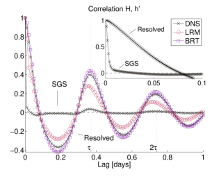
Fig. 1 (left) displays the time dependence of the autocorrelation of the resolved variable $H$ and of the SGS variable $h^{\prime}$ in the DNS. A slowly decaying oscillation is visible in the autocorrelation of $H$. The period of this oscillation is nearly equal to the time $\tau=L/\sqrt{g\mathcal{H}}\approx 0.37\,\text{day}$, required for gravity waves to pass once through the domain. This shows that the model has some intrinsic dynamics and is not dominated by forcing and diffusion. The autocorrelation of the SGS variable $h^{\prime}$ decays much faster to zero than that of $H$. The large difference in the correlation time between SGS and resolved variables indicates that the assumption of time-scale separation between x and y is met to a good agreement.

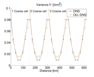
The spatial distribution of the variance of $h^{\prime}$ is displayed in Fig. 1 (right). The variance is lowest in the middle of a coarse cell, and gradually increases towards the cell boundaries. This spatial shape is explained in Appendix E as being due to a spatially decreasing autocorrelation of $h$.

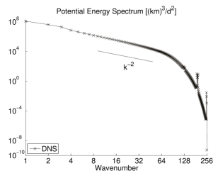
The potential-energy spectrum from the DNS is displayed in the left panel of Fig. 2. With the considered forcing and diffusion parameters one obtains an inertial range with spectral index 2 up to around wavenumber $kL/2\pi=64$. There is a small kink in the spectrum after wavenumber 3, due to the forcing acting only onto the first three modes.

The deviations from a Gaussian in the fourth order moments of $H$ and $HU$ are less than $4\%$ and $2\%$, respectively. In addition we find nearly vanishing odd moments (not shown). We conclude that the statistics of the resolved variables are close to Gaussian.

4.2 OU-DNS

As described above, the replacement $1/h\rightarrow 1/\mathcal{H}$ in the SGS nonlinearities leads to the system (33) and (34) with strictly quadratic nonlinearities, as required for the application of the SMR method. Simulations with this model reproduce the DNS data nearly perfectly (not shown).

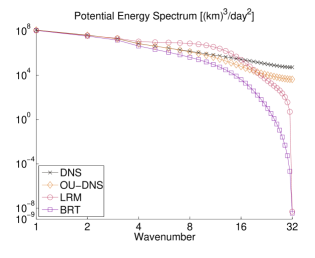
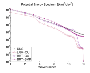
Replacing the SGS self-interactions by an empirical OU process leads to the system (43) and (44). The corresponding OU-DNS reproduces the correlations of the DNS with minor differences (not shown). The energy spectrum from the OU-DNS, projected onto the coarse grid is displayed in Fig. 2 (right). It follows the DNS spectrum for the first $7$ wavenumbers and then drops below it. This indicates a too strong damping at high wavenumbers, which seems to be due to the introduction of the deterministic part in the OU-process. The spatial variance of $h^{\prime}$ from the OU-DNS model is presented in Fig. 1 (right). It follows with small deviations the structure from the DNS model.

4.3 Low-resolution simulations without SGS parameterization

Before considering results from low-resolution simulations with the various SGS parameterizations, we first address low-resolution simulations without any parameterizations, to provide a useful reference. The time dependence of the autocorrelation function of $H$ from these simulations is shown in Fig. 1 (left). The amplitude of the oscillation of the auto-correlation from the LRM simulations is significantly weaker than from the DNS and has a relative error of $6.3\%$, computed for time lags between $0$ and $1$ day. The corresponding oscillation from the BRT simulation is slightly stronger correlated with that from the DNS, with a relative error of $2.3\%$. The corresponding period matches that from the DNS whereas that from the LRM simulation is shorter. Comparing the corresponding energy spectra in Fig. 2 (right) one can see that the energy from the BRT simulation is overall less than from the DNS, and that the spectrum is steeper. In contrast to this, LRM simulations yield too much energy between wavenumbers 4 and 15, and too little at smaller scales. At all scales LRM simulations yield more energy than the BRT simulations.

The relative errors in Table 1 show that the LRM simulation significantly overestimates the all statistical moments, the fourth moment in $HU$ even by $111.9\%$. The BRT simulation yields moments that are too small, in the case of the fourth moment by $29\%$.

We also verified numerically that in order to reproduce the spectra of the first 32 wavenumbers in the DNS with $N=512$ grid points, it is possible to perform low-resolution DNS with at least 256 spatial points. However, further reducing the number of points in the low-resolution DNS significantly corrupts the spectra of the first 32 wavenumbers. Thus, this demonstrates the need for SGS parameterizations if one wants to reduce the spatial resolution beyond $N=256$.

4.4 Low-resolution simulations with SGS parameterization

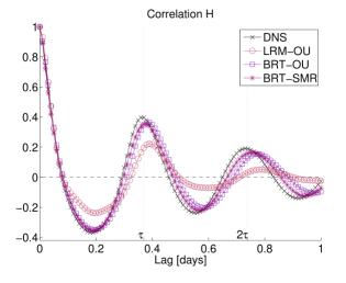
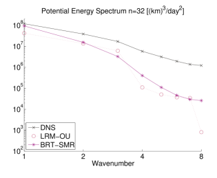
Energy spectrum. The potential-energy spectra obtained from low-resolution simulations with the different parameterizations are shown in Fig. 3 (right). The overall qualitative behavior of the shallow-water layer can be reproduced with the SMR parameterization but there is too much energy in scales up to around wavenumber $12$ and too little energy in higher wavenumbers. On the other hand, the bare truncation model with empirical stochastic corrections (BRT-OU) and the low-resolution model (LRM-OU) do not reproduce all the details of the spectra sufficiently accurately. In particular, the LRM-OU spectrum contains significantly too little energy in all wave numbers. The BRT-OU simulation can reproduce the true spectrum well in the first $15$ wavenumbers but fails completely at higher wavenumbers.

Moments. The statistical moments from the various simulations are summarized in Table 1. In general all closures show high relative errors, the empirical OU parameterizations underestimate and the SMR parameterization overestimates the moments. Errors in the $HU$-moments are smallest for the low-resolution simulation using the SMR parameterization. In the $H$-moments BRT-SMR has lower errors than LRM-OU but larger than BRT-OU. The BRT-SMR model overestimates the fluctuations in the coarse $H$-variable, which is consistent with the result for potential energy spectra discussed above. This implies that the SGS stochastic forcing representing the energy backscatter is too strong.

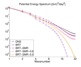
Improvement of Energy Balance. To further improve the performance of our SGS parametrization using the stochastic mode reduction, we consider BRT-SMR model with reduced SGS stochastic forcing. This is motivated by the fact that there are several assumptions in the SMR approach (e.g. time-scale separation, representing the fast variables to the leading order by the OU process, polynomial form approximation of the interaction terms in the equation for momentum). Thus, we consider BRT-SMR models where the stochastic part in the SMR parameterization is reduced by 40% or completely neglected. Stochastic terms in the SMR parametrization represent the energy backscatter of small scales onto resolved large scales. It has been recognized that proper modeling of this phenomena is particularly important in the context of geophysical turbulence (see e.g. [42, 43, 5]). Therefore, we study how well the SMR parametrization reproduces this process and whether various approximations introduced in the context of applying the SMR to the shallow water equation impose additional sensitivity of the BRT-SMR model to the stochasticity of the closure.

The reduction of the stochastic part by $40\%$ (defining BRT-SMR-0.6) significantly reduces the error in the variance of $H$ to $2.9\%$ and of $HU$ to $-5.2\%$, see Table 1. To avoid extensive tuning of the BRT-SMR model, we consider the uniform SGS noise reduction of both variables. Alternatively, SGS noises on $H$ and $HU$ can be reduced by a different percentage, thus further optimizing the performance of the BRT-SMR model. With the choice of the 40% reduction of SGS noise, the performance in the energy spectrum can be improved for the first $8$ wave numbers, but for higher wave numbers the energy content drops, see Fig. 4. However, we wold like to emphasize that the first 8 wavenumbers contain approximately $97\%$ of the potential energy. From Fig. 4 it is also visible that already the deterministic part of the closure can significantly improve the spectrum as compared to BRT.

Correlation. The time autocorrelations from low-resolution simulations (BRT or LRM) with either the empirical OU or the SMR parameterization are depicted in Fig. 3 (left). One can see that application of the SMR parameterizations leads reproducing the autocorrelation from the DNS with small differences in amplitude. The relative error of the correlation is $3.4\%$. Application of the OU parameterization in the LRM leads to simulations with an oscillation in the autocorrelation that is too weak in amplitude and exhibits a small phase shift, whereas use of the OU approach in the BRT leads to simulations with an autocorrelation similar to that obtained with the SMR parameterization. The relative error of the correlation is $10.5\%$ for the LRM-OU simulation and $6.6\%$ for the BRT-OU simulation. The SGS noise reduction in the BRT-SMR-0.6 model does not significantly affect the correlation function (not depicted for this model). The correlation function for the BRT-SMR-0.6 overlaps with the correlation function computed using the BRT-SMR. This can be intuitively understood since the correlation function in many stochastic models is determined primarily by the strength of the deterministic terms.

4.5 Scale adaptivity

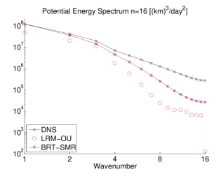
The advantage of the SMR parameterization is that it can be adapted easily to changes in the model setup, and in many situations it does not have to be recalculated. This has been investigated by considering larger averaging intervals of $\;n=16,\;32$ , resulting in different spatial resolutions $N_{c}=N/n=16,\;32$. To adjust the SMR closure to the changed resolution, we use (96) and (98) from the Appendix D. Note that no re-determination of the model is necessary. In contrast to this, no modification rule exists for the empirical closures in the BRT-OU and the LRM-OU model. We keep those parameterizations unchanged for the considered cases. Whereas the LRM-OU remains stable, the BRT-OU is unstable in both cases.

The potential energy spectra from integrations of the resulting stable models are displayed in Fig. 5. For comparison the corresponding DNS projection is shown as well. In both cases integration of the low-resolution models with SGS parameterization yield less energy in the resolved flow than the DNS. However, application of the SMR SGS parameterization leads to better agreement with the DNS, especially for $n=16$. Both low-resolution simulations can capture the time correlation well (not shown).

5 Conclusion

The applicability of subgrid-scale (SGS) parameterizations to a wide range of parameters of a dynamical system such as the atmosphere, and their ability to be easily used at different model configurations, requires that they are based on first principles as much as possible. Stochastic mode reduction (SMR) as suggested by [37, 35, 38], i.e. homogenization applied to a system with its nonlinear fast-variable self-interactions replaced by an empirical Ornstein-Uhlenbeck (OU) process, is a promising option in this direction. Geophysical applications of the SMR so far were performed always in spectral space [16, 15]. However, in many applications, such as ocean modeling or regional climate modeling, SGS parameterizations in physical space are required. In order to construct such parameterization we use the local approach suggested by [12, 13], and tested within the framework of the Burgers equation. A central aspect of this approach is the discrimination, within a finite-volume formulation of the high-resolution dynamics, between slowly varying spatial averages, that are resolved explicitly, and more rapidly varying deviations from those, that are to be parameterized.

As a next step towards the application of this technique to real atmospheric flows, our work validates the applicability of the SMR in the context of one-dimensional shallow-water (1DSW) flow. This introduces two general features. (1) Gravity waves are included as well as (2) high-order non-polynomial nonlinearities that generally affect compressible flows. After the validation of the required time-scale separation between local averages and small-scale flow, the latter issue has been handled by replacing, in all dynamical terms affecting or affected by the fast small-scale flow, the inverse of the water-column height by the inverse of its global equilibrium value. This limits the corresponding nonlinearities to quadratic. Further replacing all small-scale self-interactions by an empirical OU process yields a representation of the dynamics that allows model simulations in rather good agreement with simulations of the unmodified 1DSW equations. We could hence proceed and apply the homogenization technique to obtain an explicit low-resolution model for the local averages, with an SMR SGS parameterization of the small-scale flow coupling only a small number of neighboring cells.

This model has been validated against data from high-resolution simulations of 1DSW flow. It is shown that the SMR SGS parameterization improves the energy spectrum at the smaller resolved scales in comparison with both simulations without SGS parameterizations and simulations using an empirical OU SGS parameterization. In the error of some statistical moments no clear benefit of the SMR SGS parameterization is present. However, we demonstrated that the error can be considerably lowered by diminishing the stochasticity in the SMR closure. In particular, the variance error of the SMR SGS model can be reduced to $2.9\%$ in $H$. We also found that this comes along with less energy at high wavenumbers. We conjecture that the performance of the BRT-SMR model can be improved further by empirically adjusting the coefficients of the SMR SGS parametrization. Finally, we also show that the closure can easily be adapted to changes in the model parameters. This enables a scale awareness, which allows to utilize the SMR SGS parameterization for different spatial resolutions and leads to improvements compared to empirical SGS schemes.

In a related study within the framework of the Lorenz 96 model, [59] have recently demonstrated parameter-awareness of a parameterization derived using response theory [63] by changing the time-scale separation between resolved and unresolved scales. How far this extends to our setting, where scale-adaptivity is considered with regard to the number of resolved modes, remains to be investigated. Moreover, as shown by [62] for comparatively simple models, the SGS scheme of [63] does outperform the SMR parameterization at smaller time lags, but on longer time scales it converges to the SMR result in the limit of infinite time scale separation. Still, it would be interesting to extend the work of [10] by comparing both approaches in more complex applications.

Motivated by the DIA closure of [17, 19] applied a stochastic modeling approach accounting for memory effects of the turbulent eddies and constructed SGS parameterization from a high-resolution simulation. The resulting SGS model is local in spectral space and includes linear eddy drain viscosity and stochastic backscatter viscosity. The same approach was successfully used by [28, 29] to construct scale-aware SGS parameterizations, which reproduce the spectra exactly. Interestingly, the SMR provides additional nonlinear deterministic correction terms and multiplicative noise terms. Such terms might become important in situations where effects due to topography, intermittency or large-scale flow are relevant. In addition, the scaling laws found by [28, 29] for the eddy viscosities suggest that similar scaling laws might be valid for the parameters of the OU process in Fourier space, used in the SMR approach. This might improve further the results on scale-adaptivity presented here.

Potentially an issue is that we had to increase diffusivity in order to stabilize the low-resolution model with SMR SGS parameterization. This is a well known issue with purely empirical SGS parameterizations (e,g, [1]). In the present semi-analytical approach it might be overcome by using the energy conserving discretization of [14]. As pointed out by [36] there is a connection between energy conservation by the discretized nonlinearities and the cubic damping term in the SMR SGS parameterization. Indeed, in the studies of [16, 15, 12] the discrete treatment of the nonlinear terms conserves energy and the resulting SMR SGS schemes are stable.

Even from the present results, however, we conclude that it appears worthwhile further moving towards the application of the SMR SGS parameterizations to low-resolution simulations in general compressible flows. Next step would be to increase the complexity by considering two-dimensional shallow-water flow and by including rotational effects. Such system contains dispersive inertial gravity waves as well as geostrophic balanced flow. One interesting question in this regard is if the effect of high-frequency, small-scale gravity waves on the large-scale gravity waves and geostrophic flow can be parameterized using the present local SMR approach.

Acknowledgments

We want to thank the reviewers for their comments and suggestions which helped to improve the draft version of the manuscript. The code for the SGS parameterizations is available upon request. MZ, SD and IT thank the German Research Foundation (DFG) for partial support through grant DO 1819/1-1. IT thanks for partial support by the grant ONR N00014-17-1-2845. UA thanks DFG for partial support through grant AC 71/7-1.

Appendix A Interaction coefficients

To define the interaction coefficients in (33), (34), the following notation is used

$$\left(L_{lm}^{xz}z_{m},B^{xxz}_{lmn}x_{m}z_{n},B^{xzz}_{lmn}z_{m}z_{n}\right) =\begin{cases}\left(L^{Hz},B^{Hxz},B^{Hzz}\right)&\text{ if }x_{l}\text{ denotes }H_{I}\\ \left(L^{HUz},B^{HUxz},B^{HUzz}\right)&\text{ if }x_{l}\text{ denotes }HU_{I}\end{cases}\,,$$ (71)

$$\left(L_{lm}^{zz}z_{m},L_{lm}^{zx}x_{m}\right) =\begin{cases}\left(L^{h^{\prime}z},L^{h^{\prime}x}\right)&\text{ if }z_{l}\text{ denotes }h^{\prime}_{i}\\ \left(L^{hu^{\prime}z},L^{hu^{\prime}x}\right)&\text{ if }z_{l}\text{ denotes }hu^{\prime}_{i}\end{cases}\,,$$ (72)

$$\left(B^{zxx}_{lmn}x_{m}x_{n},B^{zxz}_{lmn}x_{m}z_{n},B^{zzz}_{lmn}z_{m}z_{n}\right) =\begin{cases}\left(B^{h^{\prime}xx},B^{h^{\prime}xz},B^{h^{\prime}zz}\right)&\text{ if }z_{l}\text{ denotes }h^{\prime}_{i}\\ \left(B^{hu^{\prime}xx},B^{hu^{\prime}xz},B^{hu^{\prime}zz}\right)&\text{ if }z_{l}\text{ denotes }hu^{\prime}_{i}\end{cases}\,,$$ (73)

with $I\in\{0,1,...,N_{c}-1\}$ and $i\in\{0,1,...,N-1\}$. The linear interaction coefficients read

$$L^{Hz}= -\frac{1}{2n\Delta x}\left(hu^{\prime}_{n(I+1)}+hu^{\prime}_{n(I+1)-1}-hu^{\prime}_{nI}-hu^{\prime}_{nI-1}\right)$$ (74)

$$+\frac{\nu}{n\Delta x^{2}}\left(h^{\prime}_{n(I+1)}-h^{\prime}_{n(I+1)-1}-h^{\prime}_{nI}+h^{\prime}_{nI-1}\right)$$

$$L^{HUz}= \frac{\nu}{n\Delta x^{2}}\left(hu^{\prime}_{n(I+1)}-hu^{\prime}_{n(I+1)-1}-hu^{\prime}_{nI}+hu^{\prime}_{nI-1}\right)$$ (75)

$$L^{h^{\prime}x}= -\frac{1}{2\Delta x}\left(HU_{I[i+1]}-HU_{I[i-1]}\right)+\frac{\nu}{\Delta x^{2}}\left(H_{I[i-1]}-2H_{I[i]}+H_{I[i+1]}\right)$$ (76)

$$+\frac{1}{2n\Delta x}\left(HU_{I[i]+1}-HU_{I[i]-1}\right)-\frac{\nu}{n\Delta x^{2}}\left(H_{I[i]+1}-2H_{I[i]}+H_{I[i]-1}\right)$$ (77)

$$L^{hu^{\prime}x}= \frac{\nu}{\Delta x^{2}}\left(HU_{I[i-1]}-2HU_{I[i]}+HU_{I[i+1]}\right)$$ (78)

$$-\frac{\nu}{n\Delta x^{2}}\left(HU_{I[i]+1}-2HU_{I[i]}+HU_{I[i]-1}\right)$$ (79)

$$L^{h^{\prime}z}= -\frac{1}{2\Delta x}\left(hu^{\prime}_{i+1}-hu^{\prime}_{i-1}\right)+\frac{\nu}{\Delta x^{2}}\left(h^{\prime}_{i-1}-2h^{\prime}_{i}+h^{\prime}_{i+1}\right)-L^{Hz}$$ (80)

$$L^{hu^{\prime}z}= \frac{\nu}{\Delta x^{2}}\left(hu^{\prime}_{i-1}-2hu^{\prime}_{i}+hu^{\prime}_{i+1}\right)-L^{HUz}\,,$$ (81)

where in (80), (81) the terms $L^{Hz}$ and $L^{HUz}$ are given in (74), (75), but with the index $I$ replaced by $I[i]$. The nonlinear interaction coefficients read

$$B^{Hxz} =B^{Hzz}=B^{h^{\prime}xx}=B^{h^{\prime}xz}=B^{h^{\prime}zz}=0$$ (82)

$$B^{HUxz} =-\frac{1}{n\Delta x}\Bigg{[}\frac{1}{\mathcal{H}}\Big{(}HU_{I+1}hu^{\prime}_{n(I+1)}+HU_{I}hu^{\prime}_{n(I+1)-1}$$ (83)

$$-HU_{I}hu^{\prime}_{nI}-HU_{I-1}hu^{\prime}_{nI-1}\Big{)}$$

$$+\frac{g}{2}\left(H_{I+1}h^{\prime}_{n(I+1)}+H_{I}h^{\prime}_{n(I+1)-1}-H_{I}h^{\prime}_{nI}-H_{I-1}h^{\prime}_{nI-1}\right)\Bigg{]}$$

$$B^{HUzz}= -\frac{1}{2n\Delta x}\Bigg{[}\frac{1}{\mathcal{H}}\left((hu^{\prime}_{n(I+1)})^{2}+(hu^{\prime}_{n(I+1)-1})^{2}-(hu^{\prime}_{nI})^{2}-(hu^{\prime}_{nI-1})^{2}\right)$$ (84)

$$+\frac{g}{2}\left((h^{\prime}_{n(I+1)})^{2}+(h^{\prime}_{n(I+1)-1})^{2}-(h^{\prime}_{nI})^{2}-(h^{\prime}_{nI-1})^{2}\right)\Bigg{]}$$

$$B^{hu^{\prime}xx}= -\frac{1}{2\Delta x}\left(\frac{1}{\mathcal{H}}\left(HU_{I[i+1]}^{2}-HU_{I[i-1]}^{2}\right)+\frac{g}{2}\left(H_{I[i+1]}^{2}-H_{I[i-1]}^{2}\right)\right)$$ (85)

$$+\frac{1}{2n\Delta x}\left[\frac{1}{\mathcal{H}}\left(HU_{I[i]+1}^{2}-HU_{I[i]-1}^{2}\right)+\frac{g}{2}\left(H_{I[i]+1}^{2}-H_{I[i]-1}^{2}\right)\right]$$ (86)

$$B^{hu^{\prime}xz}= -\frac{1}{\Delta x}\left[\frac{1}{\mathcal{H}}\left(HU_{I[i+1]}hu^{\prime}_{i+1}-HU_{I[i-1]}hu^{\prime}_{i-1}\right)+\frac{g}{2}\left(H_{I[i+1]}h^{\prime}_{i+1}-H_{I[i-1]}h^{\prime}_{i-1}\right)\right]$$

$$-B^{HUxz}$$ (87)

$$B^{hu^{\prime}zz}= -\frac{1}{2\Delta x}\left(\frac{1}{\mathcal{H}}\left((hu^{\prime}_{i+1})^{2}-(hu^{\prime}_{i-1})^{2}\right)+\frac{g}{2}\left((h^{\prime}_{i+1})^{2}-(hu^{\prime}_{i-1})^{2}\right)\right)-B^{HUzz}\,,$$ (88)

where in (87), (88) the terms $B^{HUxz}$ and $B^{HUzz}$ are given in (83), (84), but with the index $I$ replaced by $I[i]$.

Appendix B Null-space projection and inverse of the OU backward Fokker-Planck operator

To determine the projection operator $P$ and the inverse operator $L_{1}^{-1}$ one can consider an auxiliary process described by the backward FPE $\partial_{t}\chi=L_{1}\chi$ with the conditional PDF $\chi(\tilde{\textbf{y}},0\mid\textbf{y},\tau)$. The invariant measure of this process $p_{s}(\tilde{\textbf{y}})=\underset{\tau\rightarrow-\infty}{\text{lim}}\chi(\tilde{\textbf{y}},0\mid\textbf{y},\tau)$ defines the projection operator

$$\left(P\thinspace g\right)(\textbf{x})=\int d\textbf{y}\;g(\textbf{x},\textbf{y})p_{s}(\textbf{y})=\langle g(\textbf{x},\textbf{y})\rangle\;,$$ (89)

with the expectation $\langle\cdot\rangle$ of $g(\textbf{x},\textbf{y})$ with respect to the invariant measure $p_{s}$. The inverse operator $L_{1}^{-1}$ applied onto a function $f(\textbf{x},\textbf{y})$ is found to be given by

$$\left(L_{1}^{-1}\thinspace f\right)(\textbf{x},\textbf{y})=\int_{0}^{\infty}d\tau\int d\textbf{y}\;f(\textbf{x},\tilde{\textbf{y}})\chi(\tilde{\textbf{y}},\tau\mid\textbf{y},0)\;.$$ (90)

Both operators applied consecutively yield

$$\left(PgL_{1}^{-1}\thinspace f\right)(\textbf{x})= \int d\textbf{y}\;g(\textbf{x},\textbf{y})p_{s}(\textbf{y})\int_{0}^{\infty}d\tau\int d\tilde{\textbf{y}}\;f(\textbf{x},\tilde{\textbf{y}})\chi(\tilde{\textbf{y}},\tau\mid\textbf{y},0)$$

$$= \int_{0}^{\infty}d\tau\int d\textbf{y}\;g(\textbf{x},\textbf{y})p_{s}(\textbf{y})\int d\tilde{\textbf{y}}\;f(\textbf{x},\tilde{\textbf{y}})\chi(\tilde{\textbf{y}},\tau\mid\textbf{y},0)$$

$$= \int_{0}^{\infty}d\tau\;\left\langle g(\textbf{x},\textbf{y})f(\textbf{x},\tilde{\textbf{y}}(\tau))\right\rangle\,,$$ (91)

where in the lagged covariance in the last line $\tilde{\textbf{y}}(\tau)$ is understood to be an OU trajectory with initial condition $\tilde{\textbf{y}}(0)=\textbf{y}$.

Appendix C Solvability condition

The solvability condition (56) can be rewritten to $Pb^{x}_{i}\partial_{x_{i}}p^{0}=0$ since $p^{0}=p^{0}(\textbf{x})$. It is fulfilled if the even stronger condition $Pb^{x}_{i}=0$ holds. This is the case here. Using (45), defining

$$\kappa_{jk}=R_{jl}R_{km}\langle y_{l}y_{m}\rangle$$ (92)

and inserting the transformation $\textbf{z}=R\textbf{y}$, one obtains with $\langle y_{i}\rangle=0$

$$Pb^{x}_{i}=B^{xyy}_{ijk}\langle y_{j}y_{k}\rangle=B^{xzz}_{ijk}\kappa_{jk}=B^{xzz}_{ijj}\kappa_{jj}\;.$$ (93)

We have used in the last step that $B^{xzz}_{ijk}=B^{xzz}_{ijk}\delta_{jk}$, as can be seen from Appendix A. Since $B^{xzz}_{ijj}\kappa_{jj}$ is a difference between fluxes at the right and at the left of a cell, the total sum over $i$ vanishes

$$\sum_{i}B^{xzz}_{ijj}\kappa_{jj}= 0\;.$$ (94)

The homogeneity of $\langle y_{l}y_{m}\rangle$ implies that each element in the sum is identical and thus must vanish. This proofs the solvability condition.

Appendix D The SMR SGS parameterization for changed resolution

The SMR SGS parameterization can be adapted to different coarse grid resolutions without any recalculation. This can be achieved by collecting interaction coefficients proportional to different powers of $n$. For example the linear coefficients $L^{yx}$ can be written as $L^{yx}=\tilde{L}^{yx}+\frac{1}{n}\hat{L}^{yx}$, where $\hat{L}^{yx}$ results from all terms in $L^{yx}$ multiplied by $\frac{1}{n}$ and $\tilde{L}^{yx}$ from terms independent of $n$. Similarly all other coefficients can be split in this way, in particular we have $L^{xy}=\frac{1}{n}\hat{L}^{xy}$, $B^{xxy}=\frac{1}{n}\hat{B}^{xxy}$, etc.. This separation leads to the deterministic closure

$$\beta_{i}= \left(\frac{1}{n}\hat{L}^{xy}_{mj}+\frac{1}{n}\hat{B}^{xxy}_{mlj}x_{l}\right)\frac{1}{n}\hat{B}^{xxy}_{imk}(C_{S})_{jk}$$

$$+\left(\left[\tilde{L}_{mo}^{yx}+\frac{1}{n}\hat{L}_{mo}^{yx})\right]x_{o}+\left[\tilde{B}_{mop}^{yxx}+\frac{1}{n}\hat{B}_{mop}^{yxx}\right]x_{o}x_{p}\right)\frac{1}{n}\left(\hat{L}_{ik}^{xy}+\hat{B}_{ijk}^{xxy}x_{j}\right)\langle\textbf{y}\textbf{y}^{T}\rangle^{-1}_{mn}(C_{S})_{nk}$$

$$+\frac{1}{n}\hat{B}_{ijk}^{xyy}\left[\tilde{B}_{mpo}^{yxy}+\frac{1}{n}\hat{B}_{mpo}^{yxy}\right]x_{p}\langle\textbf{y}\textbf{y}^{T}\rangle^{-1}_{mn}(C_{T})_{onjk}$$ (95)

$$= \frac{1}{n}\tilde{\beta}_{i}+\frac{1}{n^{2}}\hat{\beta}_{i}$$ (96)

where in the last steps the results are summarized with respect to the power of $n$. The effective stochastic closure analogously yields

$$d\xi_{i}\approx \frac{1}{n}\sqrt{2\hat{B}_{ijn}^{xyy}(C_{T})_{jnkl}\hat{B}_{ikl}^{xyy}}dW^{1}_{i}+\frac{1}{n}\sqrt{2\left(\hat{L}^{xy}_{in}+\hat{B}^{xxy}_{ijn}x_{j}\right)(C_{S})_{nk}\left(\hat{L}^{xy}_{ik}+\hat{B}^{xxy}_{ilk}x_{l}\right)}dW^{2}_{i}$$ (97)

$$= \frac{1}{n}d\hat{\xi}_{i}\,.$$ (98)

Appendix E Spatial shape of the SGS variance

In continuous space the surface-height mean in the first coarse cell, with length $L_{c}$, and the corresponding SGS deviations can be written as

$$H=\frac{1}{L_{c}}\int_{0}^{L_{c}}h(x)\;dx\;, h^{\prime}(x)=h(x)-H\;.$$ (99)

This leads to spatial dependence in the variance of $h^{\prime}$

$$\overline{h^{\prime}(x)^{2}}-\overline{h^{\prime}}^{2}=\overline{h(x)^{2}}-2\overline{h(x)H}+\overline{H^{2}}-\overline{h^{\prime}}^{2}\;,$$ (100)

Due to spatial homogeneity of $h(x)$ and $\overline{h^{\prime}}=0$, only the second term can be assumed to be spatially dependent. Now by assuming an exponentially decaying spatial correlation $\overline{h(x)h(x^{\prime})}\sim\text{exp}\left(-\alpha|x-x^{\prime}|\right)$, with a decay rate $\alpha>0$, the middle term becomes

$$\overline{h(x)H}= \frac{1}{L_{c}}\int_{0}^{L_{c}}\overline{h(x)h(x^{\prime})}\;dx^{\prime}$$

$$\sim \frac{1}{L_{c}}\left\{\int_{0}^{x}\text{exp}\left[\alpha(x^{\prime}-x)\right]\;dx^{\prime}+\int_{x}^{L_{c}}\text{exp}\left[\alpha(x-x^{\prime})\right]\;dx^{\prime}\right\}$$

$$= \frac{1}{\alpha L_{c}}\left\{2-\text{e}^{-\alpha x}-\text{e}^{\alpha(x-L_{c})}\right\}$$

$$= \frac{2}{\alpha L_{c}}\left\{1-\text{e}^{-\frac{\alpha L_{c}}{2}}\text{cosh}\left[\alpha\left(x-\frac{L_{c}}{2}\right)\right]\right\}\;,$$ (101)

describing the characteristic U-shape of the fine variable variance in the first coarse cell $x\in[0,L_{c}]$. The same considerations hold for all other coarse cells.

Table 1: First column in both tables shows the spatially averaged second ($k=2$) and fourth ($k=4$) order centered statistical moments values of DNS. The other columns contain the relative errors of different low-resolution simulations. Upper table for $H$ and lower table for $HU$.

$H$	DNS	LRM	BRT	LRM-OU	BRT-OU	BRT-SMR	BRT-SMR-0.6	BRT-SMR-0.0
$k=2$	2.846 $(\text{km})^{2}$	0.138	-0.167	-0.589	-0.125	0.195	0.029	-0.049
$k=4$	23.56 $(\text{km})^{4}$	0.542	-0.290	-0.821	-0.207	0.455	0.080	-0.079

$HU$	DNS	LRM	BRT	LRM-OU	BRT-OU	BRT-SMR	BRT-SMR-0.6	BRT-SMR-0.0
$k=2$	2082 $(10^{3}(\text{km})^{2}/\text{d})^{2}$	0.255	-0.159	-0.597	-0.141	0.099	-0.052	-0.124
$k=4$	1.277E+07 $(10^{3}(\text{km})^{2}/\text{d})^{4}$	1.119	-0.274	-0.834	-0.251	0.185	-0.119	-0.247

Table 2: Summary of the different models used

DNS	Direct Numerical Simulation with spatial resolution of $N$ cells
	$\dot{x}_{i}=\varrho^{x}_{i}+a^{x}_{i}(\textbf{x})+b^{xz}_{i}(\textbf{x},\textbf{z})$; $\dot{z}_{i}=b^{z}_{i}(\textbf{x},\textbf{z})+c^{z}_{i}(\textbf{z})$
BRT	Bare-Truncation Model with spatial resolution of $N_{c}=N/n$
	$\dot{x}_{i}=\varrho^{x}_{i}+a^{x}_{i}(\textbf{x})$
LRM	Low-Resolution Model
	DNS with spatial resolution of $Nc=N/n$.
OU-DNS	DNS with $\frac{1}{h}$-approximation and SGS self-interactions replaced by an OU process
	$\dot{x}_{i}=\varrho^{x}_{i}+a^{x}_{i}(\textbf{x})+b^{x}_{i}(\textbf{x},\textbf{y})$, $\dot{y}_{i}=b^{y}_{i}(\textbf{x},\textbf{y})+\Lambda_{ij}y_{j}+\Sigma_{i}\dot{W}_{i}$.
BRT-OU	BRT with empirical Ornstein-Uhlenbeck parameterization
	$dx_{i}=\left(\varrho^{x}_{i}+a^{x}_{i}(\textbf{x})+\tilde{\Gamma}_{ij}\hat{x}^{I}_{j}\right)dt+\tilde{\sigma_{i}}dW_{i}$.
LRM-OU	LRM with empirical Ornstein-Uhlenbeck parameterization
BRT-SMR	BRT with Stochastic Mode Reduction parameterization
	$dx_{i}=\left[\varrho^{x}_{i}+a^{x}_{i}(\textbf{x})+\beta_{i}(\textbf{x})\right]dt+d\xi_{i}(\textbf{x})$
BRT-SMR-0.6	BRT-SMR with stochastic forcing reduced to $60\%$
	$dx_{i}=\left[\varrho^{x}_{i}+a^{x}_{i}(\textbf{x})+\beta_{i}(\textbf{x})\right]dt+0.6d\xi_{i}(\textbf{x})$.
BRT-SMR-0.0	BRT-SMR without stochastic forcing
	$dx_{i}=\left[\varrho^{x}_{i}+a^{x}_{i}(\textbf{x})+\beta_{i}(\textbf{x})\right]dt$

Figure 1: Left: spatially averaged time autocorrelation of the resolved variable $H$ and SGS variable $h^{\prime}$. Results from the DNS and two low-resolution simulations without SGS parameterizations (LRM and BRT). On the time axis the characteristic gravity wave time $\tau$ is marked, see Sec. 4 4.1. In the upper right corner a shorter time interval is presented, which resolves the decay of $h^{\prime}$. Right: the variance of the SGS variable $h^{\prime}$ for $32$ fine grid points and an averaging interval $n=8$. Results from the DNS and OU-DNS.

Figure 2: Left: the potential energy spectrum computed from $h$ in the DNS. Right: the potential energy spectrum computed from $H$ in the DNS, OU-DNS and two low-resolution simulations without SGS parameterizations (LRM and BRT).

Figure 3: The spatially averaged time autocorrelation (left) and the potential energy spectrum (right) from DNS and three low-resolution simulations with SGS parameterizations (LRM-OU, BRT-OU, BRT-SMR).

Figure 4: The potential energy spectrum in DNS, BRT, BRT-SMR, BRT-SMR with a damped stochastic forcing $d\xi\rightarrow 0.6d\xi$ (BRT-SMR-0.6) and BRT-SMR with neglected stochastic forcing $d\xi\rightarrow 0$ (BRT-SMR-0.0).

Figure 5: The Spectrum for an averaging interval of $n=16$ (left) and $n=32$ (right) in DNS, LRM-OU and BRT-SMR. The simulations with LRM-OU and BRT-SMR have a resolution of $N_{c}=32$ (left) and $N_{c}=16$ (right).

References

- [1] U Achatz and G Schmitz. On the Closure Problem in the Reduction of Complex Atmospheric Models by PIPs and EOFs: A Comparison for the Case of a Two-Layer Model with Zonally Symmetric Forcing. Journal of the Atmospheric Sciences, 54(20):2452–2474, 1997.
- [2] Ulrich Achatz and Grant Branstator. A Two-Layer Model with Empirical Linear Corrections and Reduced Order for Studies of Internal Climate Variability. Journal of the Atmospheric Sciences, 56(17):3140–3160, 1999.
- [3] Ulrich Achatz, Ulrike Löbl, Stamen I. Dolaptchiev, and Andrey Gritsun. Fluctuation–Dissipation Supplemented by Nonlinearity: A Climate-Dependent Subgrid-Scale Parameterization in Low-Order Climate Models. Journal of the Atmospheric Sciences, 70(6):1833–1846, jun 2013.
- [4] Ludwig Arnold, Peter Imkeller, and Yonghui Wu. Reduction of deterministic coupled atmosphere-ocean models to stochastic ocean models: A numerical case study of the Lorenz-Maas system, volume 18. 2003.
- [5] J. Berner, G. J. Shutts, M. Leutbecher, and T. N. Palmer. A Spectral Stochastic Kinetic Energy Backscatter Scheme and Its Impact on Flow-Dependent Predictability in the ECMWF Ensemble Prediction System. Journal of the Atmospheric Sciences, 66(3):603–626, 2009.
- [6] Judith Berner, Ulrich Achatz, Lauriane Batté, Lisa Bengtsson, Alvaro De La Cámara, Hannah M. Christensen, Matteo Colangeli, Danielle R.B. Coleman, Daaaan Crommelin, Stamen I. Dolaptchiev, Christian L.E. Franzke, Petra Friederichs, Peter Imkeller, Heikki Järvinen, Stephan Juricke, Vassili Kitsios, François Lott, Valerio Lucarini, Salil Mahajaajaajan, Timothy N. Palmer, Cécile Penland, Mirjajana Sakradzijaja, Jin Song Von Storch, Antje Weisheimer, Michael Weniger, Paul D. Williams, and Jun Ichi Yano. Stochastic parameterization toward a new view of weather and climate models. Bulletin of the American Meteorological Society, 98(3):565–587, 2017.
- [7] R Buizza, M Miller, and TN Palmer. Stochastic representation of model uncertainties in the ECMWF Ensemble Prediction System. Quarterly Journal of the Royal Meteorological Society, 125(560):2887–2908, oct 1999.
- [8] Alexei Chekhlov and Victor Yakhot. Kolmogorov turbulence in a random-force-driven Burgers equation: Anomalous scaling and probability density functions. Physical Review E, 52(5):5681–5684, 1995.
- [9] Timothy Delsole. Stochastic models of quasigeostrophic turbulence. Surveys in Geophysics, 25(2):107–149, 2004.
- [10] Jonathan Demaeyer and S Vannitsem. Comparison of stochastic parameterizations in the framework of a coupled ocean-atmosphere model. 01 2018.
- [11] Jonathan Demaeyer and Stéphane Vannitsem. Stochastic parametrization of subgrid-scale processes in coupled ocean-atmosphere systems: benefits and limitations of response theory. Quarterly Journal of the Royal Meteorological Society, 143(703):881–896, jan 2017.
- [12] S. I. Dolaptchiev, U. Achatz, and I. Timofeyev. Stochastic closure for local averages in the finite-difference discretization of the forced Burgers equation. Theoretical and Computational Fluid Dynamics, 27(3-4):297–317, 2013.
- [13] Stamen I. Dolaptchiev, Ilya Timofeyev, and Ulrich Achatz. Subgrid-scale closure for the inviscid Burgers-Hopf equation. Communications in Mathematical Sciences, 11(3):757–777, 2013.
- [14] Ulrik S. Fjordholm, Siddhartha Mishra, and Eitan Tadmor. Well-balanced and energy stable schemes for the shallow water equations with discontinuous topography. Journal of Computational Physics, 230(14):5587–5609, 2011.
- [15] Christian Franzke and Andrew J Majda. Low-Order Stochastic Mode Reduction for a Prototype Atmospheric GCM. Journal of the Atmospheric Sciences, 63(2):457–479, 2006.
- [16] Christian Franzke, Andrew J Majda, and Eric Vanden-Eijnden. Low-Order Stochastic Mode Reduction for a Realistic Barotropic Model Climate. Journal of the Atmospheric Sciences, 62(6):1722–1745, jun 2005.
- [17] J. S. Frederiksen and A. G. Davies. Eddy Viscosity and Stochastic Backscatter Parameterizations on the Sphere for Atmospheric Circulation Models. Journal of Atmospheric Sciences, 54:2475–2492, October 1997.
- [18] J. S. Frederiksen, M. R. Dix, and A. G. Davies. The effects of closure-based eddy diffusion on the climate and spectra of a gcm. Tellus A, 55(1):31–44, 2003.
- [19] J. S. Frederiksen and S. M. Kepert. Dynamical Subgrid-Scale Parameterizations from Direct Numerical Simulations. Journal of Atmospheric Sciences, 63:3006–3019, November 2006.
- [20] JS Frederiksen. Subgrid-scale parameterizations of eddy-topographic force, eddy viscosity, and stochastic backscatter for flow over topography. JOURNAL OF THE ATMOSPHERIC SCIENCES, 56(11):1481–1494, JUN 1 1999.
- [21] Crispin Gardiner. Stochastic Methods. Springer-Verlag Berlin Heidelberg, 4 edition, 2009.
- [22] Dale B. Haidvogel and Aike Beckmann. Numerical Ocean Circulation Modeling. Imperial College Press, London, 1999.
- [23] K. Hasselmann. Stochastic climate models Part I. Theory. Tellus, 28(6):473–485, jan 1976.
- [24] J. Honerkamp. Stochastic Dynamical Systems: Concepts, Numerical Methods, Data Analysis. Wiley-VCH, 1994.
- [25] Peter Imkeller and Jin-Song von Storch, editors. Stochastic Climate Models. Birkhäuser Basel, Basel, 2001.
- [26] R. Z. Khasminsky. A limit theorem for the solutions of differential equations with random right-hand sides. Theory Prob. Applications, 11:390–406, 1966.
- [27] R. Z. Khasminsky. On stochastic processes defined by differential equations with a small parameter. Theory Prob. Applications, 11:211–228, 1966.
- [28] V. Kitsios, J. S. Frederiksen, and M. J. Zidikheri. Subgrid Model with Scaling Laws for Atmospheric Simulations. Journal of Atmospheric Sciences, 69:1427–1445, April 2012.
- [29] V. Kitsios, J. S. Frederiksen, and M. J. Zidikheri. Scaling laws for parameterisations of subgrid eddy-eddy interactions in simulations of oceanic circulations. Ocean Modelling, 68:88–105, August 2013.
- [30] Dmitri Kondrashov, S. Kravtsov, A. W. Robertson, and M. Ghil. A hierarchy of data-based ENSO models. Journal of Climate, 18(21):4425–4444, 2005.
- [31] Robert H. Kraichnan. The structure of isotropic turbulence at very high reynolds numbers. Journal of Fluid Mechanics, 5(4):497–543, 1959.
- [32] S. Kravtsov, D. Kondrashov, and M. Ghil. Multilevel Regression Modeling of Nonlinear Processes: Derivation and Applications to Climatic Variability. Journal of Climate, 18(21):4404–4424, nov 2005.
- [33] T. G. Kurtz. A limit theorem for perturbed operator semigroups with applications to random evolution. J. Funct. Anal., 12:55–67, 1973.
- [34] Nicholas J. Lutsko, Isaac M. Held, and Pablo Zurita-Gotor. Applying the Fluctuation–Dissipation Theorem to a Two-Layer Model of Quasigeostrophic Turbulence. Journal of the Atmospheric Sciences, 72(8):3161–3177, 2015.
- [35] A. Majda, I. Timofeyev, and E. Vanden-Eijnden. A priori tests of a stochastic mode reduction strategy. Physica D: Nonlinear Phenomena, 170(3-4):206–252, 2002.
- [36] Andrew J Majda, Christian Franzke, and Daan Crommelin. Normal forms for reduced stochastic climate models. Proceedings of the National Academy of Sciences of the United States of America, 106(10):3649–53, 2009.
- [37] Andrew J. Majda, Ilya Timofeyev, and Eric Vanden Eijnden. A mathematical framework for stochastic climate models. Communications on Pure and Applied Mathematics, 54(8):891–974, 2001.
- [38] Andrew J. Majda, Ilya Timofeyev, and Eric Vanden-Eijnden. Systematic Strategies for Stochastic Mode Reduction in Climate. Journal of the Atmospheric Sciences, 60(14):1705–1722, 2003.
- [39] Detlev Majewski, Dörte Liermann, Peter Prohl, Bodo Ritter, Michael Buchhold, Thomas Hanisch, Gerhard Paul, Werner Wergen, and John Baumgardner. The Operational Global Icosahedral–Hexagonal Gridpoint Model GME: Description and High-Resolution Tests. Monthly Weather Review, 130(2):319–338, 2002.
- [40] Adam H. Monahan and Joel Culina. Stochastic averaging of idealized climate models. Journal of Climate, 24(12):3068–3088, 2011.
- [41] Matthew Newman, Prashant D. Sardeshmukh, Christopher R. Winkler, and Jeffrey S. Whitaker. A Study of Subseasonal Predictability. Monthly Weather Review, 131(8):1715–1732, 2003.
- [42] T. N. Palmer. A nonlinear dynamical perspective on model error: A proposal for non-local stochastic-dynamic parametrization in weather and climate prediction models. Quarterly Journal of the Royal Meteorological Society, 127(572):279–304, 2001.
- [43] T N Palmer, R Buizza, F Doblas-Reyes, T Jung, M Leutbecher, G J Shutts, M Steinheimer, and A Weisheimer. Stochastic Parametrization and Model Uncertainty. ECMWF Technical Memoranda, 598:1–42, 2009.
- [44] G. Papanicolaou. Some probabilistic problems and methods in singular perturbations. Rocky Mountain J. Math, 6:653–673, 1976.
- [45] Grigorios A. Pavliotis and Andrew M. Stuart. Multiscale Methods, volume 53 of Texts Applied in Mathematics. Springer New York, New York, NY, 2008.
- [46] Kathy Pegion and Prashant D. Sardeshmukh. Prospects for Improving Subseasonal Predictions. Monthly Weather Review, 139(11):3648–3666, 2011.
- [47] V. Petoukhov, A. Ganopolski, V. Brovkin, M. Claussen, A. Eliseev, C. Kubatzki, and S. Rahmstorf. CLIMBER-2: A Climate System Model of Intermediate Complexity. Part I: Model Description and Performance for Present Climate. Climate Dynamics, 16:1–17, 2000.
- [48] Martin Pieroth, Stamen I. Dolaptchiev, Matthias Zacharuk, Andrey Gritsun, and Ulrich Achatz. Climate-Dependence in Empirical Parameters of Subgrid-Scale Parameterizations using the Fluctuation-Dissipation Theorem. Journal of the Atmospheric Sciences, 2018. submitted.
- [49] Stephen B. Pope. Turbulent Flows. Cambridge University Press, Cambridge, 2000.
- [50] P. Rípodas, A. Gassmann, J. Förstner, D. Majewski, M. Giorgetta, P. Korn, L. Kornblueh, H. Wan, G. Zängl, L. Bonaventura, and T. Heinze. Icosahedral Shallow Water Model (ICOSWM): results of shallow water test cases and sensitivity to model parameters. Geoscientific Model Development Discussions, 2(1):581–638, 2009.
- [51] M. Satoh, T. Matsuno, H. Tomita, H. Miura, T. Nasuno, and S. Iga. Nonhydrostatic icosahedral atmospheric model (NICAM) for global cloud resolving simulations. Journal of Computational Physics, 227(7):3486–3514, 2008.
- [52] Glenn Shutts. A kinetic energy backscatter algorithm for use in ensemble prediction systems. Quarterly Journal of the Royal Meteorological Society, 131(612):3079–3102, 2005.
- [53] W.C. Skamarock and Coauthors. A Description of the Advanced Research WRF Version 3. Technical Report NCAR/TN-475+STR, NCAR, 2008.
- [54] Roland B. Stull, editor. An Introduction to Boundary Layer Meteorology. Springer Netherlands, Dordrecht, 1988.
- [55] Geoffrey K Vallis. Atmospheric and Oceanic Fluid Dynamics: Fundamentals and Large-Scale Circu- lation. 2006.
- [56] W. T M Verkley. A maximum entropy approach to the problem of parametrization. Quarterly Journal of the Royal Meteorological Society, 137(660):1872–1886, 2011.
- [57] W. T M Verkley, P. C. Kalverla, and C. A. Severijns. A maximum entropy approach to the parametrization of subgrid processes in two-dimensional flow. Quarterly Journal of the Royal Meteorological Society, 142(699):2273–2283, 2016.
- [58] W. T M Verkley and C. A. Severijns. The maximum entropy principle applied to a dynamical system proposed by Lorenz. European Physical Journal B, 87(1), 2014.
- [59] Gabriele Vissio and Valerio Lucarini. A proof of concept for scale-adaptive parameterizations: the case of the Lorenz ’96 model. Quarterly Journal of the Royal Meteorological Society, 2017.
- [60] Andrew J. Weaver, Michael Eby, Edward C. Wiebe, Cecilia M. Bitz, Phil B. Duffy, Tracy L. Ewen, Augustus F. Fanning, Marika M. Holland, Amy MacFadyen, H. Damon Matthews, Katrin J. Meissner, Oleg Saenko, Andreas Schmittner, Huaxiao Wang, and Masakazu Yoshimori. The UVic earth system climate model: Model description, climatology, and applications to past, present and future climates. Atmosphere-Ocean, 39(4):361–428, 2001.
- [61] Christopher R. Winkler, Matthew Newman, and Prashant D. Sardeshmukh. A linear model of wintertime low-frequency variability. Part I: Formulation and forecast skill. Journal of Climate, 14(24):4474–4494, 2001.
- [62] Jeroen Wouters, Stamen Iankov Dolaptchiev, Valerio Lucarini, and Ulrich Achatz. Parameterization of stochastic multiscale triads. Nonlinear Processes in Geophysics, 23(6):435–445, 2016.
- [63] Jeroen Wouters and Valerio Lucarini. Disentangling multi-level systems: averaging, correlations and memory. Journal of Statistical Mechanics: Theory and Experiment, 2012(03):P03003, 2012.
- [64] Jeroen Wouters and Valerio Lucarini. Multi-level Dynamical Systems: Connecting the Ruelle Response Theory and the Mori-Zwanzig Approach. Journal of Statistical Physics, 151(5):850–860, 2013.