Simple Load Balancing

Abstract.

We consider the following load balancing process for $m$ tokens distributed arbitrarily among $n$ nodes connected by a complete graph: In each time step a pair of nodes is selected uniformly at random. Let $\ell_{1}$ and $\ell_{2}$ be their respective number of tokens. The two nodes exchange tokens such that they have $\lceil(\ell_{1}+\ell_{2})/2\rceil$ and $\lfloor(\ell_{1}+\ell_{2})/2\rfloor$ tokens, respectively. We provide a simple analysis showing that this process reaches almost perfect balance within $\mathrm{O}\mathopen{}\mathclose{{}\left(n\log{n}+n\log{\Delta}}\right)$ steps, where $\Delta$ is the maximal initial load difference between any two nodes.

1. Introduction

We consider a load balancing problem for $m$ tokens on $n$ identical nodes connected by a complete graph. Each node starts with some number of tokens and the objective is to distribute the tokens as evenly as possible. A natural and simple process to reach this goal is as follows: At each time step, a pair of nodes $(u,v)$ is chosen uniformly at random and their loads (number of tokens) are balanced as evenly as possible. We provide a simple and elementary proof that this process takes, w.h.p. (with high probability), $\mathrm{O}\mathopen{}\mathclose{{}\left(n\log{n}+n\log{\Delta}}\right)$ time steps to reach almost perfect balance. Here, $\Delta$ is the maximal initial load difference between any two nodes and almost perfect balance means that all nodes have a load in $\set{\lfloor\varnothing\rceil-1,\lfloor\varnothing\rceil,\lfloor\varnothing\rceil+1}$, where $\varnothing=m/n$ and $\lfloor\varnothing\rceil$ is $\varnothing$ rounded to the nearest integer.

Related Work

There is a vast body of literature on load balancing, even when considering only theoretical results. As it is beyond the scope of this article to provide a complete survey, we focus on results for discrete load balancing on complete graphs and processes with sequential (or at least independent) load balancing actions. For an overview of results on general graphs, processes with multiple correlated load balancing actions (like the so-called diffusion model), and other variants we refer the reader to [6, 1].

We should first like to note that the result we prove may almost be considered folklore and variants of it have been proved in different contexts, for example in [4] (who use this to prove results in a specific distributed computational model called population model) or [6] (who study load balancing on general graphs; see below). Nevertheless, we believe that this load balancing setting is important enough (variants of it appearing as building blocks in many distributed algorithms) that there is merit in providing a dedicated, intuitive, and elementary proof.

A related load balancing model is the matching model, also known as the dimension exchange model. Here, each time step an arbitrary matching of nodes is given and any two matched nodes balance their load. In our case, the matching in each round consists of a single edge chosen independently and uniformly at random. A rather general way to analyze this model on arbitrary graphs was introduced by [5]. The authors studied how far the discrete load balancing process diverges from its continuous counterpart (where tokens can be split arbitrarily). This idea was later extended and used by [6] to prove the currently best bounds for the matching model (and others). For the complete graph and assuming that each round a random matching is used, their results imply a bound of $\mathrm{O}\mathopen{}\mathclose{{}\left(\log m}\right)$ rounds (which translates to $\mathrm{O}\mathopen{}\mathclose{{}\left(n\log m}\right)$ time steps in our model, as they use matchings of size $\Theta\mathopen{}\mathclose{{}\left(n}\right)$) to reduce the difference between maximum and minimum load to some (unspecified) constant. The time bound holds with probability $1-\exp\bigl{(}-{(\ln n)}^{\Theta\mathopen{}\mathclose{{}\left(1}\right)}\bigr{)}$, which is slightly weaker than our probabilistic guarantee.

Another related strain of literature considers discrete, sequential load balancing, but with the restriction that only one token can move per time step. [3] considered a simple local search process in this scenario: Tokens are activated by an independent exponential clock of rate $1$. Upon activation, a token samples a random node and moves there if that node’s load is smaller than the load at the token’s current host node. It has recently been proved [2] that this process reaches perfect balance in $\mathrm{O}\mathopen{}\mathclose{{}\left(\log n+\log(n)\cdot n^{2}/m}\right)$ time (both in expectation and with high probability), which is asymptotically tight.

1.1. Model and Notation

Assume $m$ indistinguishable tokens are distributed arbitrarily among $n$ nodes of a complete graph. Define the load vector $\bm{L}(t)=\mathopen{}\mathclose{{}\left(\ell_{1}(t),\dots,\ell_{n}(t)}\right)\in\mathbb{Z}^{n}$ at time $t$, where $\ell_{i}(t)$ is the number of tokens (load) assigned to node $i$ at time $t$. The discrepancy $\Delta\bm{L}(t)$ at time $t$ is the maximal load difference between any two nodes. Let $\Delta=\Delta\bm{L}(0)$ be the initial discrepancy. We define $\varnothing=m/n$ as the average load and use $\lfloor\varnothing\rceil$ to denote the average load rounded to the nearest integer.

Given the load vector $\bm{L}(t)$ at time $t$, our load balancing process performs the following actions during time step $t$: (1) Two nodes $u$ and $v$ are selected uniformly at random without replacement. (2) Their loads are updated according to $\ell_{u}(t+1)=\mathopen{}\mathclose{{}\left\lceil\mathopen{}\mathclose{{}\left(\ell_{u}(t)+\ell_{v}(t)}\right)/2}\right\rceil$ and $\ell_{v}(t+1)=\mathopen{}\mathclose{{}\left\lfloor\mathopen{}\mathclose{{}\left(\ell_{u}(t)+\ell_{v}(t)}\right)/2}\right\rfloor$. For the sake of the analysis we assume that tokens are ordered (arbitrarily) on each node. Based on this order, we define the height $h_{b}(t)$ of a token $b$ at time $t$ as the number of tokens that precede $b$ in this order. The normalized height $\hat{\operatorname{h}}_{b}\mathopen{}\mathclose{{}\left({t}}\right)=\operatorname{h}_{b}\mathopen{}\mathclose{{}\left({t}}\right)-\lfloor\varnothing\rceil$ enumerates the tokens relative to the rounded average $\lfloor\varnothing\rceil$. Furthermore, we initially assume that balancing operations between two nodes operate in stack mode, where the topmost tokens of the node with higher load are moved to the node with lower load (see Item 2). For the second part of our analysis (Phase 2: Improving Individual Tokens) we assume that balancing operations operate in skip mode, where every second token is moved (see Item 2). Finally, in the third part of our analysis (Phase 3: Fine Tuning), we assume that the excess tokens are first shuffled before the balancing operates in stack mode. Note that the mode does not influence the balancing process but merely facilitates the analysis.

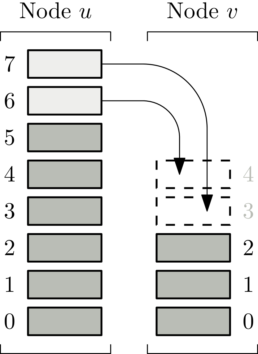
(a) Stack Mode

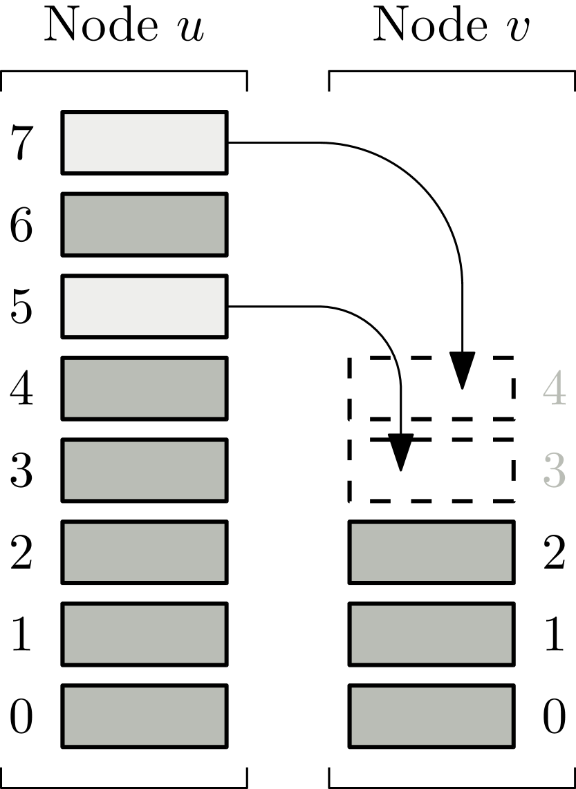
(b) Skip Mode (c) Illustration of the different modes assumed for balancing operation during the analysis.

2. Analysis

We split the analysis into three phases. In Phase 1: Potential Function Analysis we use a potential function argument to show that, w.h.p., it takes $\mathrm{O}\mathopen{}\mathclose{{}\left(n\log{n}+n\log{\Delta}}\right)$ time steps until at most $n/2$ nodes have a load larger than $\varnothing+\Theta\mathopen{}\mathclose{{}\left(1}\right)$. In Phase 2: Improving Individual Tokens we look at individual tokens and prove that, w.h.p., it takes $\mathrm{O}\mathopen{}\mathclose{{}\left(n\log{n}}\right)$ more time steps until all nodes have load at most $\varnothing+\Theta\mathopen{}\mathclose{{}\left(1}\right)$. Finally, in Phase 3: Fine Tuning we prove that, w.h.p., it takes $\mathrm{O}\mathopen{}\mathclose{{}\left(n\log{n}}\right)$ further time steps until the maximum load is at most $\lfloor\varnothing\rceil+1$. Using a symmetry-based argument we get a similar bound on the minimum load and, thus, the following theorem.

Theorem 1.

Let $\bm{L}(0)\in\mathbb{N}_{0}^{n}$ be the initial load vector of the load balancing process on $n$ nodes and let $\Delta=\Delta\bm{L}(0)$ be the initial discrepancy. Let furthermore $T$ be the first time when all nodes have load in $\set{\lfloor\varnothing\rceil-1,\lfloor\varnothing\rceil,\lfloor\varnothing\rceil+1}$. With high probability, $T=\mathrm{O}\mathopen{}\mathclose{{}\left(n\log\Delta+n\log n}\right)$. Observe that Theorem 1 is tight for polynomial $\Delta$: with constant probability there are nodes that are not selected at all during the first $\mathrm{o}\mathopen{}\mathclose{{}\left(n\log{n}}\right)$ time steps.

2.1. Phase 1: Potential Function Analysis

We analyze the process with the potential function defined via $$\Phi(\bm{\ell})=\sum_{i=1}^{n}{\mathopen{}\mathclose{{}\left(\ell_{i}-\varnothing}\right)}^{2}$$ (1) for a load vector $\bm{\ell}\in\mathbb{N}_{0}^{n}$.

Lemma 1.

Let $T_{1}$ be the first time step for which $\Phi(\bm{L}(T_{1}))<n$. W.h.p., $T_{1}=\mathrm{O}\mathopen{}\mathclose{{}\left(n\log{n}+n\log{\Delta}}\right)$.

Proof.

We start by analyzing the expected change of the potential during one time step. Let $\delta(\bm{\ell},i,j)$ be the potential drop of a fixed load vector $\bm{\ell}=(\ell_{1},\dots,\ell_{n})\in\mathbb{N}_{0}^{n}$ when nodes $i$ and $j$ are balancing. Then $$\delta(\bm{\ell},i,j)={(\ell_{i}-\varnothing)}^{2}+{(\ell_{j}-\varnothing)}^{2}-{\mathopen{}\mathclose{{}\left(\mathopen{}\mathclose{{}\left\lceil\frac{\ell_{i}+\ell_{j}}{2}}\right\rceil-\varnothing}\right)}^{2}-{\mathopen{}\mathclose{{}\left(\mathopen{}\mathclose{{}\left\lfloor\frac{\ell_{i}+\ell_{j}}{2}}\right\rfloor-\varnothing}\right)}^{2}\enspace.$$ (2) We define the discretization error $r_{\ell}(i,j)$ as $1$ if $\ell_{i}+\ell_{j}$ is odd and $0$ otherwise. This allows us to expand and simplify the above expression to get $\displaystyle\delta(\bm{\ell},i,j)$ $\displaystyle=\frac{{\mathopen{}\mathclose{{}\left(\ell_{i}-\ell_{j}}\right)}^{2}-r_{\ell}(i,j)^{2}}{2}\geq\frac{{\mathopen{}\mathclose{{}\left(\ell_{i}-\ell_{j}}\right)}^{2}}{2}-1/2\enspace.$ (3) Equation 3 implies that the potential never increases when two nodes balance (the only negative term is $-r_{\ell}(i,j)^{2}/2$, but $r_{\ell}(i,j)=1$ implies $\ell_{i}\neq\ell_{j}$ and, thus, ${(\ell_{i}-\ell_{j})}^{2}\geq 1$). We now calculate the expected potential after one time step. Each pair of nodes is chosen uniformly at random with probability $1/\binom{n}{2}$. When chosen, the potential drops by $\delta(\bm{\ell}(t),i,j)$. Therefore, $\displaystyle\operatorname{\mathbb{E}}\mathopen{}\mathclose{{}\left[{\Phi(\bm{L}(t+1))|\bm{L}(t)=\bm{\ell}}}\right]$ $\displaystyle=\sum_{i=1}^{n}\sum_{j=i+1}^{n}\frac{1}{\binom{n}{2}}\cdot\mathopen{}\mathclose{{}\left(\Phi(\bm{\ell})-\delta(\bm{\ell},i,j)}\right)$ (4) $\displaystyle\leq\Phi(\bm{\ell})-\frac{1}{2\binom{n}{2}}\sum_{i=1}^{n}\sum_{j=i+1}^{n}{\mathopen{}\mathclose{{}\left(\ell_{i}-\ell_{j}}\right)}^{2}+\frac{1}{2}\enspace.$ We now use $\sum_{i=1}^{n}\sum_{j=i+1}^{n}{\mathopen{}\mathclose{{}\left(\ell_{i}-\ell_{j}}\right)}^{2}=n\cdot\Phi(\bm{\ell})$ and obtain $\displaystyle\operatorname{\mathbb{E}}\mathopen{}\mathclose{{}\left[{\Phi(\bm{L}(t+1))|\bm{L}(t)=\bm{\ell}}}\right]$ $\displaystyle\leq\Phi(\bm{\ell})-\frac{1}{2\binom{n}{2}}\cdot n\cdot\Phi(\bm{\ell})+\frac{1}{2}\leq\mathopen{}\mathclose{{}\left(1-\frac{1}{n}}\right)\cdot\Phi(\bm{\ell})+\frac{1}{2}\enspace.$ (5) We now partition the time horizon into rounds of $n$ consecutive time steps each and look at successful rounds (in which the potential drops sufficiently). We then argue that $\mathrm{O}\mathopen{}\mathclose{{}\left(\log\mathopen{}\mathclose{{}\left(\Phi(\bm{L}(0))/n}\right)}\right)$ successful rounds suffice for the potential to drop below $n$ and that, w.h.p., we have this many successful rounds among the first $\mathrm{O}\mathopen{}\mathclose{{}\left(\log{n}+\log{\Delta}}\right)$ rounds. Let round $r$ consist of the time steps in $[r\cdot n,(r+1)\cdot n)$. We assume that the load vector $\bm{L}(r\cdot n)=\bm{\ell}$ at the beginning of round $r$ is fixed. By recursive application of Equation 5, we get $\displaystyle\operatorname{\mathbb{E}}\mathopen{}\mathclose{{}\left[{\Phi(\bm{L}((r+1)\cdot n))|\bm{L}(r\cdot n)=\bm{\ell}}}\right]$ $\displaystyle\leq{\mathopen{}\mathclose{{}\left(1-\frac{1}{n}}\right)}^{n}\cdot\Phi(\bm{\ell})+\frac{1}{2}\cdot\sum_{i=0}^{n-1}{\mathopen{}\mathclose{{}\left(1-\frac{1}{n}}\right)}^{i}$ (6) $\displaystyle\leq e^{-1}\cdot\Phi(\bm{\ell})+\frac{n}{2}\cdot\mathopen{}\mathclose{{}\left(1-e^{-1}}\right)\enspace,$ where we used the inequality ${\mathopen{}\mathclose{{}\left(1-1/n}\right)}^{n}\leq e^{-1}$. As long as $\Phi(\bm{\ell})\geq n$, the last expression is at most $$\mathopen{}\mathclose{{}\left(e^{-1}+\frac{n}{2\Phi(\bm{\ell})}\mathopen{}\mathclose{{}\left(1-e^{-1}}\right)}\right)\cdot\Phi(\bm{\ell})\leq\frac{1+e^{-1}}{2}\cdot\Phi(\bm{\ell})<\frac{3}{4}\Phi(\bm{\ell})\enspace.$$ (7) Applying the Markov inequality now gives us, for an $\bm{\ell}$ with $\Phi(\bm{\ell})\geq n$, $\displaystyle\Pr\mathopen{}\mathclose{{}\left[{\Phi(\bm{L}((r+1)\cdot n))\geq\frac{7}{8}\cdot\Phi(\bm{\ell})|\bm{L}(r\cdot n)=\bm{\ell}}}\right]$ $\displaystyle\leq\frac{6}{7}\enspace.$ (8) We define a round $r$ to be successful if $\Phi(\bm{L}((r+1)\cdot n))\leq 7/8\cdot\Phi(\bm{L}(r\cdot n))\leavevmode\nobreak\ \lor\leavevmode\nobreak\ \Phi(\bm{L}(r\cdot n))<n$ and use $\mathcal{E}_{r}$ to denote this event. Equation 8 implies $\Pr\mathopen{}\mathclose{{}\left[{\mathcal{E}_{r}}}\right]\geq 1/7$. We now argue that after at most $\rho=\log_{8/7}\mathopen{}\mathclose{{}\left(\Phi(\bm{L}(0))/n}\right)+1$ successful rounds the potential is smaller than $n$. Let $r_{\rho}$ be the $\rho$-th successful round. There are two cases. If there exists a round $r\leq r_{\rho}$ for which $\Phi(\bm{L}(r\cdot n))<n$, then $\Phi(\bm{L}(r_{\rho}))<n$ is trivially true since the potential does never increase. Otherwise, by definition of a successful round, after $\rho$ successful rounds we have $$\Phi(\bm{L}(r_{\rho}\cdot n))\leq{\mathopen{}\mathclose{{}\left(\frac{7}{8}}\right)}^{\rho}\cdot\Phi(\bm{L}(0))=\frac{7}{8}\cdot\frac{n}{\Phi(\bm{L}(0))}\cdot\Phi(\bm{L}(0))<n\enspace.$$ (9) It remains to show that, w.h.p., during the first $\mathrm{O}\mathopen{}\mathclose{{}\left(\log{n}+\log{\Delta}}\right)$ rounds at least $\rho$ rounds are successful. Let the random variable $X$ denote the number of successful rounds during the first $168\mathopen{}\mathclose{{}\left(\ln{n}+\log\Delta}\right)$ rounds. Since each round is successful with probability at least $1/7$, the random variable $X$ stochastically dominates the binomial random variable $Y\sim\operatorname{Bin}(168\mathopen{}\mathclose{{}\left(\ln{n}+\log\Delta}\right),1/7)$ (written $X\succeq Y$). Applying Chernoff bounds to $Y$ with its expected value $\mu=\operatorname{\mathbb{E}}\mathopen{}\mathclose{{}\left[{Y}}\right]=24\mathopen{}\mathclose{{}\left(\ln{n}+\log\Delta}\right)$ gives $\displaystyle\Pr\mathopen{}\mathclose{{}\left[{Y\leq\rho}}\right]$ $\displaystyle=\Pr\mathopen{}\mathclose{{}\left[{Y\leq\mathopen{}\mathclose{{}\left(1-\frac{\mu-\rho}{\mu}}\right)\mu}}\right]\leq\exp\mathopen{}\mathclose{{}\left(-\frac{{\mathopen{}\mathclose{{}\left(\mu-\rho}\right)}^{2}}{\mu^{2}}\cdot\frac{\mu}{2}}\right)\stackrel{{\scriptstyle\eqref{eq:mu-rho}}}{{\leq}}\exp\mathopen{}\mathclose{{}\left(-\frac{\mu}{8}}\right)\leq n^{-3}\enspace,$ (10) where we used the following inequality to bound $\mu-\rho$, holding for $\Delta\geq 1$: $$\rho=\log_{8/7}{\mathopen{}\mathclose{{}\left(\frac{\Phi(\bm{L}(0))}{n}}\right)}+1\leq\log_{8/7}{\mathopen{}\mathclose{{}\left(\frac{n\cdot\Delta^{2}}{n}}\right)}+1\leq\frac{2\log{\Delta}}{\log{8}/{7}}+1<12\log\Delta+1<\frac{\mu}{2}\enspace.$$ (11) Since $X\succeq Y$, Equation 10 implies that the probability of having fewer than $\rho$ successful rounds during the first $7n\cdot\mu$ time steps is smaller than $n^{-3}$. Therefore, w.h.p., $T_{1}\leq 7n\cdot\mu=\mathrm{O}\mathopen{}\mathclose{{}\left(n\log{n}+n\log{\Delta}}\right)$. ∎

2.2. Phase 2: Improving Individual Tokens

We now consider individual tokens. We start our analysis with Lemma 2, where we show that during any time step any token with normalized height larger than some constant reduces its height with probability $\Omega\mathopen{}\mathclose{{}\left(1/n}\right)$ by a constant factor. This is then used in Lemma 3 to argue that it takes at most $\mathrm{O}\mathopen{}\mathclose{{}\left(n\log{n}}\right)$ time steps for all tokens to reach a constant normalized height. For the sake of the analysis we now define which tokens are selected to be transferred when two nodes are balanced. Recall that according to the definition of the process tokens are indistinguishable and therefore arbitrary tokens may be selected. Fix a time step $t$ and assume that node $u$ interacts with node $v$. In order to balance their loads, we need to move tokens from the node with larger load to the node with smaller load (say from $u$ to $v$). To do so, we start with the token at maximal height and take every other token until we have selected required number of tokens. Then we place all tokens on node $v$ in their original order. An example for this process is sketched in Item 2. For the remainder, let $c\geq 10$ be a constant and recall that $T_{1}$ is the first time step of the second phase. The rule defined above allows us to show the following lemma.

Lemma 2.

Let $t\geq T_{1}$ and let $b$ be a token with normalized height $\hat{\operatorname{h}}_{b}\mathopen{}\mathclose{{}\left({t}}\right)>2c$. Then $\hat{\operatorname{h}}_{b}\mathopen{}\mathclose{{}\left({t+1}}\right)\leq 17/20\cdot\hat{\operatorname{h}}_{b}\mathopen{}\mathclose{{}\left({t}}\right)$ with probability at least $1/n$.

Proof.

The idea of the proof is as follows. We first argue that at any time after the first phase fewer than half of the nodes have load larger than or equal to $\varnothing+c$. This is then used to derive a lower bound on the probability that a token of normalized height larger than $2c$ takes part in balancing with a node that has load at most $\varnothing+c$. Finally, we compute the new height of the token, which yields the lemma. We now give the formal proof. Let $S(t)=\set{v}{\ell_{v}(t)\geq\varnothing+c}$ be the set of nodes which have load at least $\varnothing+c$ and suppose that $\lvert S(t)\rvert\geq n/2$. Then $$\Phi(\bm{L}(t))=\sum_{i=1}^{n}{\mathopen{}\mathclose{{}\left(\ell_{i}(t)-\varnothing}\right)}^{2}\geq\sum_{i\in S}{\mathopen{}\mathclose{{}\left(\ell_{i}(t)-\varnothing}\right)}^{2}\geq\sum_{i\in S}c^{2}\geq 100n/2>n\enspace.$$ (12) However, the potential function does not increase over time and, thus, Lemma 1 implies that $\Phi(\bm{L}(t))\leq n$ for any $t\geq T_{1}$. This is a contradiction and, therefore, $\lvert S(t)\rvert<n/2$. We now proceed to lower bound the probability that $b$ reduces its normalized height by a constant factor. Let $i$ be the node on which token $b$ is stored at time $t$. With probability $2/n$, node $i$ is selected as one of the two nodes for balancing. Let furthermore $j$ be the other node selected for balancing. Since $\lvert S(t)\rvert<n/2$, node $j$ has load at most $\varnothing+c$ with probability at least $1/2$ (independent of $i$’s selection). In that case, either $\mathopen{}\mathclose{{}\left\lfloor\frac{\ell_{i}(t)-\ell_{j}(t)}{2}}\right\rfloor$ or $\mathopen{}\mathclose{{}\left\lceil\frac{\ell_{i}(t)-\ell_{j}(t)}{2}}\right\rceil$ tokens are moved, depending on whether $(i,j)$ or $(j,i)$ are selected. Using that each other token is moved (see Item 2), carefully bounding the new height gives in both cases, regardless of whether $b$ is transfered to node $j$ or stays on node $i$, that the new height of token $b$ becomes at most $$h_{b}(t+1)\leq\ell_{j}(t)+\mathopen{}\mathclose{{}\left\lceil\frac{h_{b}(t)-\ell_{j}(t)+1}{2}}\right\rceil+1\leq\ell_{j}(t)+\frac{h_{b}(t)-\ell_{j}(t)}{2}+2=\frac{h_{b}(t)+\ell_{j}(t)+4}{2}\enspace.$$ (13) We now bound the ratio between the new and the old normalized height of token $b$. For $\ell_{j}(t)\leq\lfloor\varnothing\rceil+c$ and $h_{b}(t)\geq\lfloor\varnothing\rceil+2c$, this ratio is at most $$\frac{\hat{\operatorname{h}}_{b}\mathopen{}\mathclose{{}\left({t+1}}\right)}{\hat{\operatorname{h}}_{b}\mathopen{}\mathclose{{}\left({t}}\right)}=\frac{\frac{1}{2}\mathopen{}\mathclose{{}\left(h_{b}(t)+\ell_{j}(t)+4}\right)-\lfloor\varnothing\rceil}{h_{b}(t)-\lfloor\varnothing\rceil}=\frac{1}{2}+\frac{1}{2}\cdot\frac{\ell_{j}(t)-\lfloor\varnothing\rceil+4}{h_{b}(t)-\lfloor\varnothing\rceil}\leq\frac{1}{2}+\frac{c+4}{4c}\leq 0.85\enspace,$$ (14) where the last inequality holds since $c\geq 10$. Therefore, at any time $t\geq T_{1}$ and for any token $b$ with $\hat{\operatorname{h}}_{b}\mathopen{}\mathclose{{}\left({t}}\right)\geq 2c$, we have $\hat{\operatorname{h}}_{b}\mathopen{}\mathclose{{}\left({t+1}}\right)\leq 0.85\cdot\hat{\operatorname{h}}_{b}\mathopen{}\mathclose{{}\left({t}}\right)$ with probability at least $1/n$. ∎ We are now ready to show the main lemma for the second phase.

Lemma 3.

Let $T_{2}$ be the first time for which $\displaystyle\max_{1\leq i\leq n}\set{\ell_{i}(T_{2})}\leq\varnothing+2c$ and $\displaystyle\min_{1\leq i\leq n}\set{\ell_{i}(T_{2})}\geq\varnothing-2c$. With high probability, $T_{2}=T_{1}+\mathrm{O}\mathopen{}\mathclose{{}\left(n\log{n}}\right)$.

Proof.

We first show the claim for the maximal load and then use a coupling argument to extend the analysis to the minimal load. For the maximal load, we consider a fixed token $b$ and use Lemma 2 to define and bound the probability of a successful time step w.r.t. $b$. Then we show that this event occurs sufficiently often during the first $\mathrm{O}\mathopen{}\mathclose{{}\left(n\log{n}}\right)$ time steps such that $b$ reaches normalized height at most $2c$ with high probability. Finally, we show the claim by a union bound over all tokens of normalized height larger than $2c$. Let $b$ be an arbitrary but fixed token with $\hat{\operatorname{h}}_{b}\mathopen{}\mathclose{{}\left({t}}\right)\geq 2c$. We call a time step $t$ successful if $\hat{\operatorname{h}}_{b}\mathopen{}\mathclose{{}\left({t+1}}\right)\leq 17/20\cdot\hat{\operatorname{h}}_{b}\mathopen{}\mathclose{{}\left({t}}\right)\leavevmode\nobreak\ \lor\leavevmode\nobreak\ \hat{\operatorname{h}}_{b}\mathopen{}\mathclose{{}\left({t}}\right)\leq 2c$. From Lemma 2 we get that time step $t$ is successful with probability at least $1/n$. Note that while the behavior of two different tokens may be highly correlated, for one fixed token the lower bounds hold independently for any time step in the second phase. This allows us to leverage stochastic dominance of a binomial distribution as follows: Let the random variable $X_{b}(\tau)$ denote the number of successful time steps during the first $\tau$ time steps in the second phase. Since each time step is successful with probability at least $1/n$, the random variable $X_{b}(\tau)$ stochastically dominates the binomial random variable $Y_{b}(\tau)\sim\operatorname{Bin}(\tau,1/n)$. Applying Chernoff bounds to $Y_{b}(\tau)$ with $\tau=12n\log{n}$ gives $$\Pr\mathopen{}\mathclose{{}\left[{Y_{b}(12n\log{n})\leq\mathopen{}\mathclose{{}\left(1-\frac{3}{4}}\right)\operatorname{\mathbb{E}}\mathopen{}\mathclose{{}\left[{Y_{b}(12n\log{n})}}\right]}}\right]\leq\exp\mathopen{}\mathclose{{}\left(-\frac{1}{2}\cdot\frac{9}{16}\cdot 12\log{n}}\right)\leq n^{-3}\enspace.$$ (15) With the above mentioned stochastic dominance $X_{b}(\tau)\succeq Y_{b}(\tau)$, we get that $X_{b}(12n\log{n})\leq 3\log n$ with probability at most $n^{-3}$. It remains to show that the normalized height of $b$ after $3\log{n}$ successful time steps is at most $2c$. Observe that $\hat{\operatorname{h}}_{b}\mathopen{}\mathclose{{}\left({T_{1}}}\right)\leq\sqrt{n}$, since otherwise $\Phi(\bm{L}(T_{1}))\geq n$. Therefore, after at most $3\log{n}$ successful time steps in the second phase, the normalized height of $b$ is at most $$\hat{\operatorname{h}}_{b}\mathopen{}\mathclose{{}\left({T_{1}+12n\log{n}}}\right)\leq\max\set{\sqrt{n}\cdot{\mathopen{}\mathclose{{}\left(\frac{17}{20}}\right)}^{3\log n},2c}\leq 2c\enspace.$$ (16) We now use the union bound on the above analysis over all tokens as follows. From the bound on the potential function in Lemma 1 we obtain that after the first phase at most $n$ tokens remain above the average, since otherwise the potential would be larger than $n$. Observing that the height of a token never increases and taking the union bound over all tokens of normalized height above $2c$ gives us that all tokens have remaining height at most $2c$ after at most $12n\log{n}$ interactions with probability $1-1/n^{-2}$. We now argue an analogous bound for the minimal load. Let $\bm{\ell}\in\mathbb{Z}^{n}$ be the initial load vector of the load balancing process $\bm{L}(0)=\bm{\ell},\bm{L}(1),\bm{L}(2),\dots$ and let $-\bm{\ell}$ be the initial load vector of the load balancing process $\bm{L}^{\prime}(0)=-\bm{\ell},\bm{L}^{\prime}(1),\bm{L}^{\prime}(2),\dots$. We can couple the processes such that whenever a pair of nodes $(u,v)$ is chosen in $\bm{L}(t)$, the pair of nodes $(v,u)$ is chosen in $\bm{L}^{\prime}(t)$. This coupling ensures (determinstically) that $\ell_{i}(t)=-\ell^{\prime}_{i}(t)$ and, thus, implies $\Pr\mathopen{}\mathclose{{}\left[{\ell_{i}(t)=x}}\right]=\Pr\mathopen{}\mathclose{{}\left[{\ell^{\prime}_{i}(t)=-x}}\right]$. By applying the upper bound on the maximal load to $\bm{L}^{\prime}(T_{1}+12n\log{n})$, we get a lower bound on the minimal load in $\bm{L}(T_{1}+12n\log{n})$. Thus, $T_{2}\leq T_{1}+\mathrm{O}\mathopen{}\mathclose{{}\left(n\log{n}}\right)$, which concludes the proof. ∎

2.3. Phase 3: Fine Tuning

For the sake of the analysis of the third phase, we use the following rule to select tokens to transfer when balancing two nodes. We again assume that nodes operate like stacks, with the following additional rule: both nodes shuffle their tokens of normalized height in $\set{2,3,\dots,2c}$ (if they exist) before balancing the loads. This rule allows us to show the following lemma, our main result.

Lemma 4.

Let $T_{3}$ be the first time for which $\max_{1\leq i\leq n}\set{\ell_{i}(T_{3})}\leq\lfloor\varnothing\rceil+1$ and for which $\min_{1\leq i\leq n}\set{\ell_{i}(T_{3})}\geq\lfloor\varnothing\rceil-1$. With high probability, $T_{3}=T_{2}+\mathrm{O}\mathopen{}\mathclose{{}\left(n\log{n}}\right)$.

Proof.

We again start by analyzing the maximal load. We first show that at any time step after the second phase at least a constant fraction of nodes has load at most $\lfloor\varnothing\rceil$. Then we consider an arbitrary but fixed token $b$ with $\hat{\operatorname{h}}_{b}\mathopen{}\mathclose{{}\left({t}}\right)>1$ at time $t$ and show that with probability $\Omega\mathopen{}\mathclose{{}\left(1/n}\right)$ we have $\hat{\operatorname{h}}_{b}\mathopen{}\mathclose{{}\left({t+1}}\right)\leq 1$. This is used to show that, w.h.p., $\hat{\operatorname{h}}_{b}\mathopen{}\mathclose{{}\left({\tau}}\right)\leq 1$ for $\tau=\mathrm{O}\mathopen{}\mathclose{{}\left(n\log n}\right)$. The claim then follows from a union bound over all tokens above normalized height $1$. Fix a time step $t\geq T_{2}$ and let $\gamma$ be the fraction of nodes that have load at most $\lfloor\varnothing\rceil$ at time $t$. We use the definition of the rounded average load and Lemma 3 to compute $\displaystyle n\cdot\mathopen{}\mathclose{{}\left(\lfloor\varnothing\rceil+0.5}\right)\geq n\cdot\varnothing=\sum_{1\leq i\leq n}\ell_{i}(t)=\smashoperator[r]{\sum_{\ell_{i}(t)>\lfloor\varnothing\rceil}^{}}\ell_{i}(t)+\smashoperator[lr]{\sum_{\ell_{i}(t)\leq\lfloor\varnothing\rceil}^{}}\ell_{i}(t)$ (17) $\displaystyle{}\geq{}$ $\displaystyle\smashoperator[r]{\sum_{\ell_{i}(t)>\lfloor\varnothing\rceil}^{}}\mathopen{}\mathclose{{}\left(\lfloor\varnothing\rceil+1}\right)+\smashoperator[lr]{\sum_{\ell_{i}(t)\leq\lfloor\varnothing\rceil}^{}}\mathopen{}\mathclose{{}\left(\lfloor\varnothing\rceil-2c}\right)\geq n\cdot\mathopen{}\mathclose{{}\left(1-\gamma}\right)\cdot\mathopen{}\mathclose{{}\left(\lfloor\varnothing\rceil+1}\right)+n\cdot\gamma\cdot\mathopen{}\mathclose{{}\left(\lfloor\varnothing\rceil-2c}\right)\enspace.$ Therefore, $\gamma\geq{1}/({4c+2})$ is a constant. Similar to the analysis of the second phase, we now consider an arbitrary but fixed token $b$. Fix a time step $t\geq T_{2}$ and a token $b$ with $\hat{\operatorname{h}}_{b}\mathopen{}\mathclose{{}\left({t}}\right)>1$. Let $i$ be the node on which $b$ resides before time step $t$. We have the following events. i) Node $i$ is selected for balancing: in any time step, $i$ is selected with probability $2/n$. ii) Token $b$ becomes the top-most token: all tokens $b^{\prime}$ on node $i$ of normalized height $\hat{\operatorname{h}}_{b^{\prime}}\mathopen{}\mathclose{{}\left({t}}\right)>1$ are shuffled. Since there exist at most $2c$ such tokens after the second phase, $b$ becomes the top-most token with probability at least $1/(2c)$. iii) The other node has load at most $\lfloor\varnothing\rceil$: since the fraction of such nodes is least $\gamma$, such a node is selected as the balancing partner with probability at least $\gamma$. We say $b$ is successful in time step $t$ if all three of these events occur. Observe that in this case $\hat{\operatorname{h}}_{b}\mathopen{}\mathclose{{}\left({t+1}}\right)\leq 1$. Let $p_{b}(t)$ be the probability of a successful time step. Combining above probabilities, we get $p_{b}(t)\geq 2/n\cdot 1/(2c)\cdot\gamma=\Omega\mathopen{}\mathclose{{}\left(1/n}\right)$. We now consider $\mathrm{O}\mathopen{}\mathclose{{}\left(n\log n}\right)$ time steps after the second phase. Token $b$ is not successful at least once during these time steps with probability $$\prod_{t=1}^{\mathrm{O}\mathopen{}\mathclose{{}\left(n\log{n}}\right)}\mathopen{}\mathclose{{}\left(1-p_{b}(t)}\right)\leq{\mathopen{}\mathclose{{}\left(1-\Omega\mathopen{}\mathclose{{}\left(\frac{1}{n}}\right)}\right)}^{\mathrm{O}\mathopen{}\mathclose{{}\left(n\log{n}}\right)}\leq n^{-\Omega\mathopen{}\mathclose{{}\left(1}\right)}\enspace.$$ (18) That is, for a suitable choice of constants, $b$ reaches height $1$ after at most $\mathrm{O}\mathopen{}\mathclose{{}\left(n\log{n}}\right)$ time steps with probability $1-1/n^{3}$. The upper bound on the load now follows from a union bound, since at most $2c\cdot n$ tokens have normalized height above $1$ after the second phase. For the lower bound on the load, precisely the same argument as in the proof of Lemma 3 can be used. ∎ The proof of Theorem 1 now follows from a union bound over the results from Lemma 1 for the first phase, Lemma 3 for the second phase, and Lemma 4 for the third phase.