QCD Sum Rule for Open Strange Meson $K_{1}^{\pm}$ in Nuclear Matter

Abstract

The properties of open strange meson $K_{1}^{\pm}$ in nuclear matter are estimated in the QCD sum rule approach. We obtain a relation between the in-medium mass and width of $K_{1}^{-}$ ($K_{1}^{+}$) in nuclear matter, and show that the upper limit of the mass shift is as large as -249 (-35) MeV. The spectral modification of the $K_{1}$ meson is possible to be probed by using kaon beams at J-PARC. Such measurement together with that of $K^{*}$ will shed light on how chiral symmetry is partially restored in nuclear matter.

I Introduction

In the QCD vacuum, chiral symmetry is spontaneously broken, which leads to the non-vanishing chiral order parameters and the existence of the Nambu-Goldstone (NG) bosons. It also leads to the mass difference between the vector meson and its axial partner Weinberg:1967kj ; Shifman:1978bx . This broken symmetry is expected to have been restored in the early universe, when the temperature was very high. Furthermore, it was noted that the chiral symmetry is partially restored even in normal nuclear density so that by exciting mesons inside the nucleus one could study the precursor phenomena of chiral symmetry restoration Hatsuda:1985eb ; Brown:1991kk ; Hatsuda:1991ez ; Klingl:1997kf . Furthermore, the enhanced repulsion of the s-wave isovector pion-nucleus interaction observed in the deeply bound pionic atoms Suzuki:2002ae was shown to be a direct consequence of the reduction of the in-medium quark condensate in nuclear medium Kolomeitsev:2002gc .

According to the in-medium QCD sum rules developed in Hatsuda:1991ez , in-medium change of the four-quark condensate (the strange quark condensate) is responsible for the spectral change of the $\rho,\omega$ mesons (the $\phi$ meson). A number of experiments have since then carried out worldwide Hayano:2008vn . The KEK-PS experiments observed the invariant mass spectra of $e^{+}~{}e^{-}$ pairs from the nuclear targets and found excess signals at the lower end of the $\omega$ resonance peak that could be explained by the vector meson mass decrease of 9 $\%$ at the normal nuclear density Naruki:2005kd . The KEK-PS E325 collaboration reported evidence that the mass of the $\phi$ meson decreased by 3.4 $\%$ at normal nuclear density Muto:2005za . Further measurements of dileptons from the in-medium $\phi$-meson are planned at J-PARC E16 experiment Ichikawa:2018woh . Dilepton spectrum has the advantage of not suffering from strong interaction with the medium as the signal emerges from inside the nucleus but has the disadvantage of being low in the yield. Reactions involving hadronic final states have the opposite features. For example, CBELSA/TAPS Collaboration observed that the $\omega$ meson decreased by about 60 MeV at an estimated average nuclear density of 0.6 $\rho_{0}$ through the reaction $\gamma+A\rightarrow\omega+X\rightarrow\pi^{0}\gamma+X^{\prime}$ Trnka:2005ey . However, the signal could have been contaminated by final state interactions. Furthermore, $\omega$ and $f_{1}$ are chiral partners only in the limit where disconnected quark diagrams are neglected Gubler:2016djf and the QCD sum rule approach was found to have a large contribution from the scattering term DuttMazumder:2000ys ; Thomas:2005dc ; Leupold:2009kz , so that it is not clear if the sum rule leads to a decreasing mass. Alternative approach by the CBELSA/TAPS collaboration is to extract meson-nucleus optical potentials from near-threshold meson productions in photo- and hadro- reactions off nuclei as well as in heavy-ion reactions by focussing on mesons with small width in the vacuum ($K,\eta,\eta^{\prime},\omega,\phi$) Metag:2017yuh . The momentum distribution of mesons, excitation functions and the transparency ratios are the key experimental observables.

Motivated by recent experimental progress, one of us (SHL) have recently estimated the spectral shift of the $f_{1}$ meson, which is a chiral partner of $\omega$ in the limit where the disconnected diagrams are neglected, in the QCD sum rule approach Gubler:2016djf . Experimentally, the $f_{1}(1285)$ has been successfully identified by the CLAS collaboration in photoproduction from a proton target with a small width of $18\pm 1.4$ MeV Dickson:2016gwc , so that performing similar experiments on a nuclear target and comparing the result with that from the $\omega$ would be extremely useful for partial restoration of chiral symmetry in nuclei as suggested in Ref. Gubler:2016djf . In fact, the individual meson masses could behave differently depending on whether the hadron is in nuclear matter or at finite temperature, while the mass difference between chiral partners will only depend on the chiral order parameter and be universal Lee:2013es .

The difference between the vector and axial-vector correlation functions in the open strange channel is also an order parameter of chiral symmetry Lee:2013es . This implies that their spectral densities will become degenerate if chiral symmetry is restored. In the vacuum, the low-lying modes that couple to the vector current are $K^{*}(892)$ and $K^{*}(1410)$ while for the axial vector current they are $K_{1}(1270)$ and $K_{1}(1400)$. There is a subtlety in the nature of the two $K_{1}$ states: They are assumed to be a mixture of the ${}^{3}P_{1}$ and ${}^{1}P_{1}$ quark-antiquark pair in the quark model Suzuki:1993yc . However, if chiral symmetry is partially restored, the spectral density will tend to become degenerate so that the lowest distinctive poles in the respective current will approach each other. Therefore, in this work, we investigate the spectral modification of open strange meson $K_{1}$ through the axial-vector current in nuclear matter using QCD sum rules.

Measuring the open strange meson in the vector channel, namely the $K^{*+}$ through the decay $K^{*+}\rightarrow K^{+}+\gamma$ was suggested as a promising signal to measure the spectral change of the vector meson in Ref. Hatsuda:1997ev . Both the $K_{1}(1270)$ and the $K^{*}(892)$ have widths smaller than their non strange counter parts, namely 90 MeV and 47 MeV, respectively, compared to more than 250 MeV and 150 MeV for the $a_{1}$ and the $\rho$. At the same time, they are also chiral partners so that their mass difference is sensitive to the chiral order parameter.

We note that $K_{1}^{+}$ and $K_{1}^{-}$ become non-degenerate in nuclear medium due to the presence of nucleons which break charge conjugation invariance in the medium. There are two approaches to treat such situation in QCD sum rules. One is to project out the polarization function into definite charge conjugation states Jido:1996ia ; Suzuki:2015est . The other is to extract the ground state of each charge state from the polarization functions Kondo:2005ur . In the present paper, we take the latter method in which some parameters for $K_{1}^{-}$ are mixed into the sum rule for $K_{1}^{+}$ and vice versa.

In section II, we first discuss the QCD sum rules for $K_{1}$ meson in the vacuum. In section III, effects of nuclear matter are taken into account in the QCD sum rule through the local operators with spin. In section III, the maximum mass shift of $K_{1}^{\pm}$ meson is estimated by the pole plus continuum approximation of the spectral function. Also, by considering the modification of the width and the mass shift, we obtain a relation between the in-medium change of these two quantities. Summary and discussion are given in section IV.

II $K_{1}$ meson in vacuum

The time-ordered current correlation function of the $K_{1}$ current is given by

$$\Pi_{\mu\nu}(q)=i\int d^{4}xe^{iq\cdot x}\langle 0|T[\bar{u}\gamma_{\mu}\gamma_{5}s(x),\bar{s}\gamma_{\nu}\gamma_{5}u(0)]|0\rangle$$

$$=-i\int d^{4}xe^{iq\cdot x}\langle 0|{\rm Tr}[\gamma_{\mu}\gamma_{5}iS_{s}(x)\gamma_{\nu}\gamma_{5}iS_{u}(-x)]|0\rangle,$$

(1)

where $iS_{s}$ and $iS_{u}$ represent u-quark and s-quark propagators respectively. Including nonperturbative effect, these propagators are expanded as Furnstahl:1992pi :

$$iS^{ab}(x)=i\frac{\not{x}}{2\pi^{2}x^{4}}\delta^{ab}-\frac{m}{4\pi^{2}x^{2}}\delta^{ab}+i\frac{m^{2}\not{x}}{8\pi^{2}x^{2}}\delta^{ab}+...$$

$$+\chi^{a}(x)\chi^{b}(0)-i\frac{g}{32\pi^{2}}\frac{\not{x}\sigma_{\alpha\beta}+\sigma_{\alpha\beta}\not{x}}{x^{2}}F^{\alpha\beta}_{A}(0)t_{A}^{ab}+.,$$ (2)

where $a$, $b$ are color indices, and $\alpha$, $\beta$ Lorentz indices. The first line is the expansion of the perturbative part with respect to quark mass $m$, and the second line encodes the nonperturbative part. $\chi^{a}$ is the background field of the quark, and $F^{\alpha\beta}_{A}$ that of the gluon. Because the masses of u and d quarks are small compared to the typical QCD scale, we consider only strange quark mass to be finite in this study.

The current correlation function in the vacuum is composed of two independent functions $\Pi_{1}$ and $\Pi_{2}$ as follows:

$$\Pi_{\mu\nu}(q)=-g_{\mu\nu}\Pi_{1}(q^{2})+q_{\mu}q_{\nu}\Pi_{2}(q^{2}).$$ (3)

If the current is conserved, the two functions are related by $\Pi_{1}=q^{2}\Pi_{2}$. However, the axial current of $K_{1}$ is not conserved and $\Pi_{2}$ has contributions from pseudoscalar mesons. In principle, we may carry out QCD sum rule with either $\Pi_{1}$ or $\Pi_{2}$.

Let us first consider $\Pi_{1}$. Substituting Eq. (2) into Eq. (1), the operator product expansion (OPE) of the current correlation function is obtained up to dimension 6 as

$$\Pi_{1}(q^{2})=B_{0}Q^{2}\ln\frac{Q^{2}}{\mu^{2}}+B_{2}\ln\frac{Q^{2}}{\mu^{2}}-\frac{B_{4}}{Q^{2}}-\frac{B_{6}}{Q^{4}},$$ (4)

and

$$B_{0} = \frac{1}{4\pi^{2}}\bigg{(}1+\frac{\alpha_{s}}{\pi}\bigg{)}$$

$$B_{2} = \frac{3m_{s}^{2}}{8\pi^{2}}$$

$$B_{4} = -m_{s}\langle\bar{u}u\rangle_{0}+\frac{1}{12}\langle\frac{\alpha_{s}}{\pi}G^{2}\rangle_{0}$$

$$B_{6} = \frac{2\pi\alpha_{s}}{9}\bigg{(}\langle(\bar{s}\gamma_{\mu}\lambda^{a}s+\bar{u}\gamma_{\mu}\lambda^{a}u)(\sum_{q}\bar{q}\gamma_{\mu}\lambda^{a}q)\rangle_{0}\bigg{)}$$

$$+2\pi\alpha_{s}\bigg{(}\langle(\bar{u}\gamma_{\mu}\lambda^{a}s)((\bar{s}\gamma_{\mu}\lambda^{a}u)\rangle_{0}\bigg{)}$$

$$= \frac{32\pi\alpha_{s}}{81}\bigg{(}\langle\bar{u}u\rangle_{0}^{2}+\langle\bar{s}s\rangle_{0}^{2}\bigg{)}+\frac{32\pi\alpha_{s}}{9}\bigg{(}\langle\bar{u}u\rangle_{0}\langle\bar{s}s\rangle_{0}\bigg{)},$$

where $Q^{2}\equiv-q^{2}$, $\mu=1$ GeV is the renormalization scale, $n$ in $B_{n}$ indicates the canonical dimension of the operator, and $\langle{\cal O}\rangle_{0}$ denotes the condensate of operator $\cal{O}$ in the vacuum. We take the recently updated parameters as follows: $\alpha_{s}=0.5$, $m_{q}=4.26$ MeV, $m_{s}=117$ MeV, where both quark masses are scaled to $\mu=1$ GeV from the values at $\mu=2$ GeV given by lattice calculations in 2+1 flavors as reported in Particle Data Group Tanabashi:2018oca , $\langle\bar{u}u\rangle_{0}=(-0.262~{}{\rm GeV})^{3}$ from the Gell-Mann Oakes Renner relation $2m_{q}\langle\bar{u}u\rangle_{0}=m_{\pi}^{2}f_{\pi}^{2}$ with $m_{\pi}$ and $f_{\pi}$ being the mass and decay constant of the pion respectively, $\langle\bar{s}s\rangle_{0}=0.8\langle\bar{u}u\rangle_{0}$, and $\langle\alpha_{s}/\pi G^{2}\rangle_{0}=0.012~{}{\rm GeV}^{4}$. For the four quark operators of dimension 6, a factorization ansatz is adopted Shifman:1978bx ; Hatsuda:1991ez .

It should be noted that for the corresponding vector correlation function obtained with the current $J^{K^{*}}_{\mu}=\bar{u}\gamma_{\mu}s$, the OPE up to this order will be similar with $B_{0}^{V}=B_{0}$, $B_{2}^{V}=B_{2}$ and

$$B_{4}^{V} = +m_{s}\langle\bar{u}u\rangle_{0}+\frac{1}{12}\langle\frac{\alpha_{s}}{\pi}G^{2}\rangle_{0}$$

$$B_{6}^{V} = \frac{2\pi\alpha_{s}}{9}\bigg{(}\langle(\bar{s}\gamma_{\mu}\lambda^{a}s+\bar{u}\gamma_{\mu}\lambda^{a}u)(\sum_{q}\bar{q}\gamma_{\mu}\lambda^{a}q)\rangle_{0}\bigg{)}$$

$$+2\pi\alpha_{s}\bigg{(}\langle(\bar{u}\gamma_{\mu}\gamma^{5}\lambda^{a}s)((\bar{s}\gamma_{\mu}\gamma^{5}\lambda^{a}u)\rangle_{0}\bigg{)}$$

$$= \frac{32\pi\alpha_{s}}{81}\bigg{(}\langle\bar{u}u\rangle_{0}^{2}+\langle\bar{s}s\rangle_{0}^{2}\bigg{)}-\frac{32\pi\alpha_{s}}{9}\bigg{(}\langle\bar{u}u\rangle_{0}\langle\bar{s}s\rangle_{0}\bigg{)}.$$

The difference between the axial and the vector correlation functions is proportional to chiral symmetry breaking operators responsible for the mass difference between chiral partners. Specifically, at dimension 4, the difference is proportional to $m_{s}\langle\bar{q}q\rangle$, while at dimension 6, it is $\langle\bar{s}s\rangle\langle\bar{q}q\rangle$. Both operators are proportional to $\langle\bar{q}q\rangle$, but is dominated by the dimension 6 operator. It is interesting to note that the larger mass difference between $m_{a_{1}}-m_{\rho}\simeq 1260-770=490$ MeV compared to the corresponding mass difference in the open strange sector $m_{K_{1}}-m_{K^{*}}\simeq 1270-892=378$ MeV seems to be related to the difference in the four quark condensate $\langle\bar{q}q\rangle^{2}$ to $\langle\bar{s}s\rangle\langle\bar{q}q\rangle$ in their respective sum rules. It should be also noted that the difference in the open charm sector is dominated by the dimension 4 operators because the charm quark mass amplifies the contribution from the light quark condensate as was noted in Ref. Hilger:2011cq ; Buchheim:2014rpa .

As for the imaginary part of the correlation function, we use the phenomenological spectral function

$$\frac{1}{\pi}{\rm Im}\Pi_{1}(q^{2}) = \frac{m_{K_{1}}^{4}}{g_{K_{1}}^{2}}\delta(q^{2}-m_{K_{1}}^{2})$$ (5)

$$+(B_{0}q^{2}-B_{2})\theta(q^{2}-s_{0}),$$

where the first term on the right hand side represents the ground state and the second term the sum of all excited states, which is approximated by the continuum part starting from a threshold value $s_{0}$. The factor multiplied to the step function is obtained by the perturbative part of Eq. (4), as shown in Appendix A. The imaginary part and the real part of the correlation function are related to each other through the dispersion relation:

$$\frac{1}{\pi}\int\frac{{\rm Im}\Pi_{1}(s)}{s+Q^{2}}ds={\rm Re}\Pi_{1}(q^{2}).$$ (6)

In order to improve our approximations from both sides, namely the calculations of the real part up to dimension 6 and the step function for excited states and continuum, we take the Borel transformation defined as

$$\hat{B}\equiv\lim_{Q^{2},n\rightarrow\infty~{}Q^{2}/n\rightarrow M^{2}}\frac{1}{(n-1)!}(Q^{2})^{n}\bigg{(}-\frac{d}{dQ^{2}}\bigg{)}^{n},$$

where $M$ is called the Borel mass. For our purpose, we use

$$\hat{B}(Q^{2})^{-k}=\frac{1}{(k-1)!}\frac{1}{(M^{2})^{k}},$$ (7)

$$\hat{B}(Q^{2})^{k}\ln Q^{2}=-k!(-M^{2})^{k},$$ (8)

$$\hat{B}(Q^{2}+M_{B}^{2})^{-k}=\frac{1}{(k-1)!}\frac{1}{(M^{2})^{k}}e^{-M_{B}^{2}/M^{2}}.$$ (9)

Taking the Borel transformation has two advantages. First, as shown in Eq. (9), it introduces an exponential function in the left hand side of Eq. (6), which enhances the ground state but suppresses the continuum part. Second, the contribution from high-dimension operators in the real part of the polarization function is suppressed by an additional $1/(n-1)!$ factor.

Substituting the OPE and the phenomenological ansatz into Eq. (6), we obtain the following equation after the Borel transformation.

$$\frac{m_{K_{1}}^{4}}{g_{K_{1}}^{2}}e^{-m_{K_{1}}^{2}/M^{2}}=B_{0}M^{4}\bigg{\{}1-\bigg{(}1+\frac{s_{0}}{M^{2}}\bigg{)}e^{-s_{0}/M^{2}}\bigg{\}}$$

$$~{}~{}~{}~{}~{}~{}~{}~{}-B_{2}M^{2}\bigg{(}1-e^{-s_{0}/M^{2}}\bigg{)}-B_{4}-\frac{B_{6}}{M^{2}},$$ (10)

where the continuum part was moved to the right hand side. Differentiating Eq. (10) with respect to $1/M^{2}$, and dividing it by Eq. (10), $K_{1}$ mass is expressed as

$$m_{K_{1}}^{2}=M^{2}\frac{2B_{0}E_{2}-B_{2}E_{1}/M^{2}+B_{6}/M^{6}}{B_{0}E_{1}-B_{2}E_{0}/M^{2}-B_{4}/M^{4}-B_{6}/M^{6}},$$

(11)

where

$$E_{0} = 1-e^{-s_{0}/M^{2}},$$

$$E_{1} = 1-\bigg{(}1+\frac{s_{0}}{M^{2}}\bigg{)}e^{-s_{0}/M^{2}},$$

$$E_{2} = 1-\bigg{(}1+\frac{s_{0}}{M^{2}}+\frac{s_{0}^{2}}{2M^{4}}\bigg{)}e^{-s_{0}/M^{2}}.$$

Eq. (11) is the Borel sum rule for the $K_{1}$ mass. In principle, the physical mass should be independent of $M^{2}$. However, as mentioned above, the real part of the correlation function is truncated at dimension 6, and the excited states and continuum in the spectral function is simplified into a step function. As a result Eq. (11) depends on $M^{2}$. Then, one introduces the so-called Borel window in $M^{2}$ where the resultant $K_{1}$ mass is reliable. The smallest $M^{2}$ of the Borel window, $M^{2}_{\rm min}$, is determined from the condition that the contribution from the power corrections does not exceed 15 % of the perturbative part:

$$\bigg{|}\frac{B_{4}+B_{6}/M^{2}}{B_{0}M^{4}-B_{2}M^{2}}\bigg{|}<0.15.$$ (12)

The largest reliable $M^{2}$, $M^{2}_{\rm max}$, is determined from the condition that the contribution from the continuum does not exceed 70 %:

$$\bigg{|}\frac{B_{0}M^{2}(1-E_{1})-B_{2}(1-E_{0})}{B_{0}M^{2}-B_{2}}\bigg{|}<0.7.$$ (13)

We note that the maximum percentage is taken to be larger than in Eq. (12), which is similar to the continuum contribution for the p-wave states using the $\Pi_{1}$ sum rule Reinders:1981ww . If $M_{\rm min}^{2}$ becomes too small the large power correction spoils the stability, while if the $M_{\rm max}^{2}$ becomes too small the sensitivity of the continuum threshold is lost and one needs a large change in the continuum threshold.

Applying Eqs. (12) and (13), the Borel window is given by $1.06\leq M^{2}\leq 2.17~{}{\rm GeV^{2}}$. The continuum threshold $s_{0}$ is chosen such that the extremum of the Borel curve is close to the physical mass of $K_{1}$ ground state within the Borel window. Physically it should be close to the mass of the first excited state.

Figure 1 shows the Borel curve for the mass of $K_{1}$ at $s_{0}=2.4~{}{\rm GeV^{2}}$ together with the fractional contributions from the power corrections and the continuum. The Borel window which satisfies Eqs. (12) and (13) is shown by the black solid line. We find the minimum value of the Borel curve is consistent with the mass of $K_{1}(1270)$. The overlap strength of the current with the ground state $F_{K_{1}}\equiv m_{K_{1}}^{2}/g_{K_{1}}^{2}$ is about 0.048 ${\rm GeV^{2}}$ in this window. We note that $\sqrt{s_{0}}=1.55~{}{\rm GeV}$ is close to the mass of $K_{1}(1400)$.

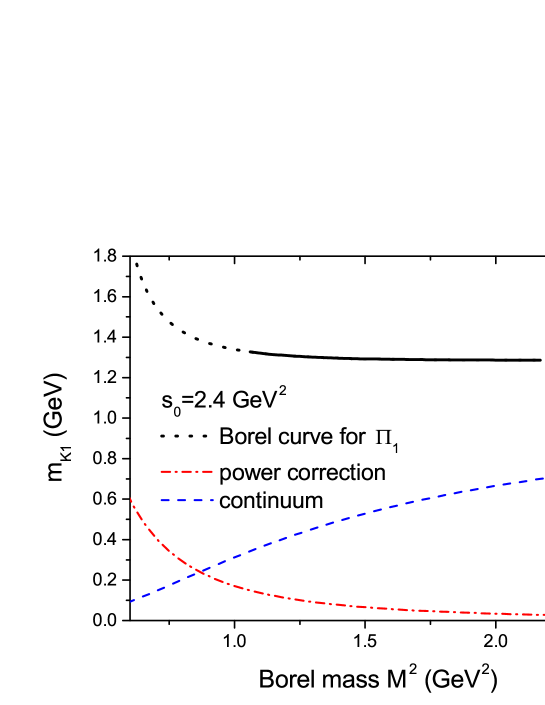
Figure 1: The Borel curve for $K_{1}$ mass from the $\Pi_{1}$ sum rule together with the fractional contributions from the power corrections and the continuum. The Borel window given in Eqs. (12) and (13) is shown by the black solid line. The unit for the mass is in GeV while for the fractional contributions it is unitless.

We can also construct a QCD sum rule with $\Pi_{2}$. The real part is then given by

$$\Pi_{2}(q^{2})=-B_{0}\ln\frac{Q^{2}}{\mu^{2}}-\frac{\tilde{B}_{2}}{Q^{2}}+\frac{\tilde{B}_{4}}{Q^{4}}+\frac{B_{6}}{Q^{6}},$$ (14)

where

$$\tilde{B}_{2} = \frac{3m_{s}^{2}}{4\pi^{2}},$$

$$\tilde{B}_{4} = m_{s}\langle\bar{s}s\rangle_{0}+\frac{1}{12}\langle\frac{\alpha_{s}}{\pi}G^{2}\rangle_{0},$$

and $B_{0}$ and $B_{6}$ are same as in $\Pi_{1}$, with $\tilde{B}_{4}=B_{4}$ in the limit $m_{s}\rightarrow 0$. However, the imaginary part will then have contribution from the pseudoscalar meson and will not be useful for our purpose as one would need additional input on the kaon properties in medium to use the corresponding sum rule to study the properties of the $K_{1}$ meson in medium. Therefore, we use the Borel curve from $\Pi_{1}$ in this study to investigate the properties of $K_{1}$ meson in nuclear matter.

III $K_{1}^{\pm}$ meson in nuclear medium

In nuclear matter, there are two modifications in the real part of the correlation function. One is the change in the values of the condensates, and the other is the appearance of operators with spin. We take into account only twist-2 terms which are dominant in OPE. (Here twist is the dimension of operator subtracted by spin.) Higher twist terms have been estimated before and are known to be less important Friman:1999wu . The degeneracy of $K_{1}^{-}$ and $K_{1}^{+}$ in the vacuum does not hold in nuclear matter due to charge symmetry breaking, which leads the odd dimensional terms in the OPE to contribute with opposite sign for the two charged states.

III.1 In-medium OPE

In the limit ${\bf q}\rightarrow 0$, the OPE in nuclear matter can be written as

$$\Pi_{1}(q^{2})=\Pi^{e}(q^{2})+q_{0}\Pi^{o}(q^{2}),$$ (15)

where

$$\Pi^{e}(q^{2}) = B_{0}Q^{2}\ln\frac{Q^{2}}{\mu^{2}}+B_{2}\ln\frac{Q^{2}}{\mu^{2}}-\frac{B_{4}^{*}}{Q^{2}}-\frac{B_{6}^{*}}{Q^{4}},$$

$$\Pi^{o}(q^{2}) = \frac{1}{3Q^{2}}(A_{1}^{u}-A_{1}^{s})\rho-\frac{2m_{N}^{2}}{3Q^{4}}(A_{3}^{u}-A_{3}^{s})\rho,$$

with

$$B_{4}^{*}=-m_{s}\langle\bar{u}u\rangle_{\rho}+\frac{1}{12}\langle\frac{\alpha_{s}}{\pi}G^{2}\rangle_{\rho},$$

$$~{}~{}~{}~{}~{}~{}~{}+\frac{m_{N}}{2}(A_{2}^{u}+A_{2}^{s})\rho$$

$$B_{6}^{*}=\frac{32\pi\alpha_{s}}{9}\bigg{\{}\langle\bar{u}u\rangle_{\rho}\langle\bar{s}s\rangle_{\rho}+\frac{\langle\bar{u}u\rangle_{\rho}^{2}+\langle\bar{s}s\rangle_{\rho}^{2}}{9}\bigg{\}}$$

$$~{}~{}~{}~{}~{}~{}~{}-\frac{5}{6}m_{N}^{3}(A_{4}^{u}+A_{4}^{s})\rho.$$ (17)

$\Pi^{e(o)}$ denotes even(odd) dimensional terms of correlation function. $\langle{\cal O}\rangle_{\rho}$ is the condensate of operator ${\cal O}$ in nuclear matter, where we use the linear density approximation: $\langle{\cal O}\rangle_{\rho}=\langle{\cal O}\rangle_{0}+\langle{\cal O}\rangle_{N}\rho$ with $\rho$ being the baryon density. $\langle\bar{u}u\rangle_{N}$, $\langle\bar{s}s\rangle_{N}$, and $\langle G^{2}\rangle_{N}$ are the nucleon matrix elements taken from Refs. Hatsuda:1991ez ; Gubler:2016djf :

$$m_{q}\langle\bar{u}u+\bar{d}d\rangle_{N}=45~{}{\rm MeV},~{}m_{s}\langle\bar{s}s\rangle_{N}=35~{}{\rm MeV},$$

$$\langle\alpha/\pi G^{2}\rangle_{N}=-8/9m_{N}.~{}~{}~{}~{}~{}~{}~{}~{}~{}~{}~{}~{}$$ (18)

$m_{N}$ is the nucleon mass, and $A_{n}^{q}(\mu^{2})=2\int_{0}^{1}x^{n-1}\{q(x,\mu^{2})+(-1)^{n}\bar{q}(x,\mu^{2})\}dx$, where $q(x,\mu^{2})$ and $\bar{q}(x,\mu^{2})$ are, respectively, quark and antiquark distribution functions in the nucleon at scale $\mu^{2}$, and are defined through the twist-two operators

$$\langle{\cal ST}(\bar{q}\gamma_{\mu_{1}}D_{\mu_{2}}...D_{\mu_{n}}q(\mu^{2}))\rangle_{N}$$

$$=(-i)^{n-1}A_{n}^{q}(\mu^{2})\frac{T_{\mu_{1}...\mu_{n}}}{2m_{N}}.$$ (19)

Here, ${\cal ST}$ means ‘symmetric and traceless’, and expressed on the right side with the tensor $T_{\mu_{1}\cdots\mu_{n}}$. For our case,

$$T_{\mu\nu} = p_{\mu}p_{\nu}-\frac{p^{2}}{4}g_{\mu\nu},$$

$$T_{\mu\nu\rho} = p_{\mu}p_{\nu}p_{\rho}-\frac{p^{2}}{6}(g_{\mu\nu}p_{\rho}++g_{\mu\rho}p_{\nu}+g_{\nu\rho}p_{\mu}),$$

$$T_{\mu\nu\rho\lambda} = p_{\mu}p_{\nu}p_{\rho}p_{\lambda}-\frac{p^{2}}{8}(g_{\mu\nu}p_{\lambda}p_{\rho}+g_{\mu\lambda}p_{\nu}p_{\rho}$$ (20)

$$+g_{\mu\rho}p_{\nu}p_{\lambda}+g_{\nu\lambda}p_{\mu}p_{\rho}+g_{\nu\rho}p_{\mu}p_{\lambda}+g_{\lambda\rho}p_{\mu}p_{\nu})$$

$$+\frac{p^{4}}{48}(g_{\mu\nu}g_{\lambda\rho}+g_{\mu\lambda}g_{\nu\rho}+g_{\mu\rho}g_{\nu\lambda}),$$

where $p_{\mu}$ is nucleon four momentum. We calculate $A_{n}^{q}(\mu^{2})$ using the MSTW parton distribution function Martin:2009iq at the scale $\mu^{2}=1~{}{\rm GeV^{2}}$, which is same as our renormalization scale of 1 GeV:

$$A_{1}^{u} = 3.0,~{}~{}~{}A_{2}^{u}=0.62,~{}~{}~{}A_{3}^{u}=0.15,~{}~{}~{}A_{4}^{u}=0.0637,$$

$$A_{1}^{s} = 0.0,~{}~{}~{}A_{2}^{s}=0.048,~{}~{}~{}A_{3}^{s}=0.00085,~{}~{}~{}A_{4}^{s}=0.0011.$$

III.2 Phenomenological side

$\Pi^{e}$ and $\Pi^{o}$ appearing in Eq. (15) are respectively even and odd under charge conjugation. Therefore, the charge even and odd states will become non-degenerate in the medium, so that we have to introduce separate physical states for the positive and negative charge states. Then the imaginary part in Eq. (15) can be written as

$$\frac{1}{\pi}{\rm Im}\Pi_{1}(q^{2})=\frac{m_{K_{1}^{-}}^{3}}{2g_{K_{1}^{-}}^{2}}\delta(q_{0}-m_{K_{1}^{-}})+\frac{m_{K_{1}^{+}}^{3}}{2g_{K_{1}^{+}}^{2}}\delta(q_{0}+m_{K_{1}^{+}})$$

$$+(B_{0}q^{2}-B_{2})\bigg{\{}\theta\bigg{(}q_{0}-\sqrt{s_{0}^{-}}\bigg{)}+\theta\bigg{(}-q_{0}-\sqrt{s_{0}^{+}}\bigg{)}\bigg{\}}.$$

(21)

in the limit ${\bf q}\rightarrow 0$. Using the definition of Eq. (LABEL:pieo), we can then extract $\Pi^{e}$ and $\Pi^{o}$ separately. Since we are interested in the $K_{1}^{\pm}$ state separately, we consider the following combination of the polarization function;

$$\frac{2}{\pi}{\rm Im}(\Pi^{e}+m_{K_{1}^{+}}\Pi^{o})=\frac{m_{K_{1}^{-}}^{4}}{g_{K_{1}^{-}}^{2}}\bigg{(}1+\frac{m_{K_{1}^{+}}}{m_{K_{1}^{-}}}\bigg{)}\delta(q^{2}-m_{K_{1}^{-}}^{2})$$

$$+(B_{0}q^{2}-B_{2})\bigg{\{}(1+\frac{m_{K_{1}^{+}}}{q_{0}})\theta(q^{2}-s_{0}^{-})~{}~{}~{}~{}~{}$$

$$+(1-\frac{m_{K_{1}^{+}}}{q_{0}})\theta(q^{2}-s_{0}^{+})\bigg{\}},~{}~{}$$

$$\frac{2}{\pi}{\rm Im}(\Pi^{e}-m_{K_{1}^{-}}\Pi^{o})=\frac{m_{K_{1}^{+}}^{4}}{g_{K_{1}^{+}}^{2}}\bigg{(}1+\frac{m_{K_{1}^{-}}}{m_{K_{1}^{+}}}\bigg{)}\delta(q^{2}-m_{K_{1}^{+}}^{2})$$

$$+(B_{0}q^{2}-B_{2})\bigg{\{}(1+\frac{m_{K_{1}^{-}}}{q_{0}})\theta(q^{2}-s_{0}^{+})~{}~{}~{}~{}~{}$$

$$+(1-\frac{m_{K_{1}^{-}}}{q_{0}})\theta(q^{2}-s_{0}^{-})\bigg{\}}.~{}$$

(22)

The first equation has the resonance of $K_{1}^{-}$ and the continuum of $K_{1}^{-}$ and $K_{1}^{+}$. On the other hand, the second equation has the resonance of $K_{1}^{+}$ and the continuum of $K_{1}^{-}$ and $K_{1}^{+}$. The detailed derivation of the imaginary part and Eq. (22) is given in Appendix B. We note that the two equations in Eq. (22) reduce to Eq. (5), when $m_{K_{1}^{-}}=m_{K_{1}^{+}}$, $g_{K_{1}^{-}}=g_{K_{1}^{+}}$, and $s_{0}^{-}=s_{0}^{+}$. We can see on the left hand side of Eq. (22) that the odd dimensional terms contribute to $K_{1}^{-}$ with a positive sign and to $K_{1}^{+}$ with a negative sign. It brings about the splitting between $K_{1}^{-}$ and $K_{1}^{+}$ in nuclear matter.

III.3 In-medium QCD sum rules

The dispersion relation for each combination

$$\frac{1}{\pi}\int\frac{{\rm Im}~{}(\Pi^{e}\pm m_{K_{1}^{\pm}}\Pi^{o})ds}{s+Q^{2}}={\rm Re}~{}(\Pi^{e}\pm m_{K_{1}^{\pm}}\Pi^{o}),$$

reduces to the following equations after the Borel transformation;

$$\frac{F_{\pm}m_{\pm}^{2}}{2M^{2}}\bigg{(}1+\frac{m_{\mp}}{m_{\pm}}\bigg{)}e^{-m_{\pm}^{2}/M^{2}}$$

$$+\frac{1}{2M^{2}}\int_{s_{0}^{\pm}}^{\infty}\bigg{(}1+\frac{m_{\mp}}{\sqrt{s}}\bigg{)}(B_{0}s-B_{2})e^{-s/M^{2}}ds$$

$$+\frac{1}{2M^{2}}\int_{s_{0}^{\mp}}^{\infty}\bigg{(}1-\frac{m_{\mp}}{\sqrt{s}}\bigg{)}(B_{0}s-B_{2})e^{-s/M^{2}}ds$$

$$=B_{0}M^{2}-B_{2}-\frac{1}{M^{2}}\bigg{\{}B_{4}^{*}\pm\frac{m_{\mp}}{3}(A_{1}^{u}-A_{1}^{s})\rho\bigg{\}}$$

$$~{}~{}~{}-\frac{1}{M^{4}}\bigg{\{}B_{6}^{*}\mp\frac{2m_{\mp}m_{N}^{2}}{3}(A_{3}^{u}-A_{3}^{s})\rho\bigg{\}},$$ (24)

where $m_{K_{1}^{\pm}}$ and $m_{\pm}^{2}/g_{K_{1}^{\pm}}^{2}$ are respectively abbreviated to $m_{\pm}$ and $F_{\pm}$.

III.3.1 In-medium mass

For small nuclear density, the overlap strength, mass, and continuum threshold may be approximated as

$$F_{\pm} = F_{K_{1}}+F^{\prime}_{\pm}\rho,$$

$$m_{\pm} = m_{K_{1}}+m^{\prime}_{\pm}\rho,$$

$$s_{0}^{\pm} = s_{0}+{s^{\prime}}_{0}^{\pm}\rho.$$ (25)

Keeping only terms linearly proportional to $\rho$, Eq. (24) reduces to

$$F(M^{2})F^{\prime}_{\pm}+M(M^{2})m^{\prime}_{\pm}+S(M^{2}){s^{\prime}}_{0}^{\pm}=C_{\pm}(M^{2}),$$

(26)

where

$$F(M^{2})=-m_{K_{1}}^{2}e^{-m_{K_{1}}^{2}/M^{2}},$$

$$M(M^{2})=F_{K_{1}}m_{K_{1}}\bigg{(}-\frac{3}{2}+\frac{2m_{K_{1}}^{2}}{M^{2}}\bigg{)}e^{-m_{K_{1}}^{2}/M^{2}},$$

$$S(M^{2})=\frac{1}{2}\bigg{(}1+\frac{m_{K_{1}}}{\sqrt{s_{0}}}\bigg{)}(B_{0}s_{0}-B_{2})e^{-s_{0}/M^{2}},$$

$$C_{\pm}(M^{2})=-m_{s}\langle\bar{u}u\rangle_{N}+\frac{\alpha_{s}}{12\pi}\langle G^{2}\rangle_{N}$$

$$~{}~{}~{}+\frac{m_{N}}{2}(A_{2}^{u}+A_{2}^{s})\pm\frac{m_{K_{1}}}{3}(A_{1}^{u}-A_{1}^{s})$$

$$~{}~{}~{}+\frac{32\pi\alpha_{s}}{9M^{2}}\bigg{\{}\langle\bar{u}u\rangle_{N}\langle\bar{s}s\rangle_{0}+\langle\bar{u}u\rangle_{0}\langle\bar{s}s\rangle_{N}$$

$$~{}~{}~{}~{}~{}~{}~{}~{}~{}~{}~{}+\frac{2}{9}(\langle\bar{u}u\rangle_{N}\langle\bar{u}u\rangle_{0}+\langle\bar{s}s\rangle_{N}\langle\bar{s}s\rangle_{0})\bigg{\}}$$

$$~{}~{}~{}-\frac{5m_{N}^{3}}{6M^{2}}(A_{4}^{u}+A_{4}^{s})\mp\frac{2m_{K_{1}}m_{N}^{2}}{3M^{2}}(A_{3}^{u}-A_{3}^{s})$$

$$~{}~{}~{}+m^{\prime}_{\mp}\bigg{\{}\frac{F_{K_{1}}m_{K_{1}}}{2}e^{-m_{K_{1}}^{2}/M^{2}}\bigg{\}}$$

$$~{}~{}~{}+{s^{\prime}}_{0}^{\mp}\bigg{\{}\frac{1}{2}\bigg{(}-1+\frac{m_{K_{1}}}{\sqrt{s_{0}}}\bigg{)}(B_{0}s_{0}-B_{2})e^{-s_{0}/M^{2}}\bigg{\}}.$$

(27)

We now define $V_{\pm}(F^{\prime}_{\pm},m^{\prime}_{\pm},{s^{\prime}}_{0}^{\pm})$ from Eq. (26) as

$$V_{\pm}(F^{\prime}_{\pm},m^{\prime}_{\pm},{s^{\prime}}_{0}^{\pm})\equiv\int_{M^{2}_{\rm min}}^{M^{2}_{\rm max}}\bigg{\{}F(M^{2})F^{\prime}_{\pm}+M(M^{2})m^{\prime}_{\pm}$$

$$~{}~{}~{}~{}~{}~{}~{}~{}~{}~{}~{}~{}~{}~{}~{}~{}~{}~{}+S(M^{2}){s^{\prime}}_{0}^{\pm}-C_{\pm}(M^{2})\bigg{\}}^{2}dM^{2},$$ (28)

where $M^{2}_{\rm min}$ and $M^{2}_{\rm max}$ are the lower and upper limits of the Borel window, which are respectively taken to be 1.06 and 2.17 ${\rm GeV^{2}}$ as in the vacuum. This will be justified in the Borel analysis discussed in the next section, where we show that the most stable Borel curve has a plateau within this Borel window and that the obtained mass shift and threshold change are consistent with those calculated in this section. Though Eq. (28) is supposed to vanish in the ideal case, it is always positive because of the approximations taken both in the OPE side and in the phenomenological side. Therefore, we search for $F^{\prime}_{\pm},m^{\prime}_{\pm}$, and ${s^{\prime}}_{0}^{\pm}$ which minimize the function $V_{\pm}$, that is,

$$\frac{\partial V_{\pm}}{\partial F^{\prime}_{\pm}}=\frac{\partial V_{\pm}}{\partial m^{\prime}_{\pm}}=\frac{\partial V_{\pm}}{\partial{s^{\prime}}_{0}^{\pm}}=0.$$ (29)

These conditions result in three simultaneous linear equations as follows:

$$F^{\prime}_{\pm}\int dM^{2}F^{2}(M^{2})+m^{\prime}_{\pm}\int dM^{2}F(M^{2})M(M^{2})+{s^{\prime}}_{0}^{\pm}\int dM^{2}F(M^{2})S(M^{2}) = \int dM^{2}F(M^{2})C_{\pm}(M^{2}),$$

$$F^{\prime}_{\pm}\int dM^{2}F(M^{2})M(M^{2})+m^{\prime}_{\pm}\int dM^{2}M^{2}(M^{2})+{s^{\prime}}_{0}^{\pm}\int dM^{2}M(M^{2})S(M^{2}) = \int dM^{2}M(M^{2})C_{\pm}(M^{2}),$$

$$F^{\prime}_{\pm}\int dM^{2}F(M^{2})S(M^{2})+m^{\prime}_{\pm}\int dM^{2}M(M^{2})S(M^{2})+{s^{\prime}}_{0}^{\pm}\int dM^{2}S^{2}(M^{2}) = \int dM^{2}S(M^{2})C_{\pm}(M^{2}).$$ (30)

$F^{\prime}_{-}\rho_{0}\ ({\rm GeV^{2}})$	$m^{\prime}_{-}\rho_{0}\ ({\rm GeV})$	${s^{\prime}}_{0}^{-}\rho_{0}\ ({\rm GeV^{2}})$	$F^{\prime}_{+}\rho_{0}\ ({\rm GeV^{2}})$	$m^{\prime}_{+}\rho_{0}\ ({\rm GeV})$	${s^{\prime}}_{0}^{+}\rho_{0}\ ({\rm GeV^{2}})$
-3.09$\times 10^{-2}$	-0.249	-1.25	-2.72$\times 10^{-3}$	-0.0348	-0.234

Table 1: Results for $F^{\prime}_{\pm}\rho$, $m^{\prime}_{\pm}\rho$, and ${s^{\prime}}_{0}^{\pm}\rho$ at normal nuclear matter density $\rho=\rho_{0}=0.16~{}{\rm fm^{-3}}$. The mass shift at nuclear matter density is $\delta m_{K_{1}^{\pm}}=m^{\prime}_{\pm}\rho$.

The above equations are coupled such that $V_{+}$ is a function of $m_{-}$ and $s_{0}^{-}$ as well as of $m_{+}$ and $s_{0}^{+}$, while $V_{-}$ is a function of $m_{+}$ and $s_{0}^{+}$ as well as of $m_{-}$ and $s_{0}^{-}$. This is so because $C_{\pm}(M^{2})$ are functions of $m_{\mp}$ and $s_{0}^{\mp}$. In other words, three simultaneous linear equations for $F^{\prime}_{+}$, $m_{+}$, and ${s^{\prime}}_{0}^{+}$ are coupled with those for $F^{\prime}_{-}$, $m^{\prime}_{-}$, and ${s^{\prime}}_{0}^{-}$. We solve these equations iteratively, with the final results of $F_{\pm}{{}^{\prime}}$, $m^{\prime}_{\pm}$, and ${s^{\prime}}_{0}^{\pm}$ shown in Table 1. We find that with the obtained values, the ratios of $V_{\pm}(F^{\prime}_{\pm},m^{\prime}_{\pm},{s^{\prime}})$ in Eq. (28) to the individual terms, $\int_{M^{2}_{\rm min}}^{M^{2}_{\rm max}}(F(M^{2})F^{\prime}_{\pm})^{2}dM^{2}$, $\int_{M^{2}_{\rm min}}^{M^{2}_{\rm max}}(M(M^{2})m^{\prime}_{\pm})^{2}dM^{2}$, $\int_{M^{2}_{\rm min}}^{M^{2}_{\rm max}}(S(M^{2}){s^{\prime}}_{0}^{\pm})^{2}dM^{2}$, and $\int_{M^{2}_{\rm min}}^{M^{2}_{\rm max}}(C_{\pm}(M^{2}))^{2}dM^{2}$ are (1.8$\times 10^{-6}$, 2.2$\times 10^{-5}$, 3.8$\times 10^{-7}$, 9.5$\times 10^{-7}$) and (1.7$\times 10^{-7}$, 5.3$\times 10^{-6}$, 1.7$\times 10^{-7}$, 7.3$\times 10^{-6}$), respectively for $\pm$ states, justifying our optimization procedure.

In these calculations, $m_{K_{1}}$ and $s_{0}$ are set to be $\rm 1.27~{}GeV$ and $\rm 2.4~{}GeV^{2}$, respectively. As a result, the mass of $K_{1}^{-}$ decreases by 249 $\rm~{}MeV$ in nuclear matter, which corresponds to 20 % reduction of the mass from its vacuum value. On the other hand, the mass of $K_{1}^{+}$ decreases only by 35 $\rm~{}MeV$, which is about 3 % of its vacuum mass. Since we have neglected the in-medium width in this subsection, these numbers are the upper limits of the mass shift. Under such condition, the result indicates that $K_{1}^{-}(s\bar{u})$ ($K_{1}^{+}(\bar{s}u)$) feels attraction (repulsion) in nuclear matter. This tendency is consistent with the expectation that nuclear matter attracts (repels) the $u$-anti-quark (the $u$-quark) as in the case of charged kaons, $K^{-}(s\bar{u})$ and $K^{+}(\bar{s}u)$ Martin:1980qe .

The above results can be confirmed by using the traditional Borel stability analysis in nuclear matter as originally proposed in Ref. Hatsuda:1991ez . Shown in Figure 2 are the Borel curves for the $K_{1}$ mass in the vacuum (the black curve) and those in the medium. The most stable Borel curve for $K_{1}^{+}$ occurs at $s_{0}=2.4$ GeV² with a slight decrease of the mass, while that for the $K_{1}^{-}$ occurs at a much smaller threshold with a large reduction of the mass consistent with the previous optimization method. Furthermore, one finds that for both of the charge states, the most stable curves have plateaux and extremums within the given Borel window.

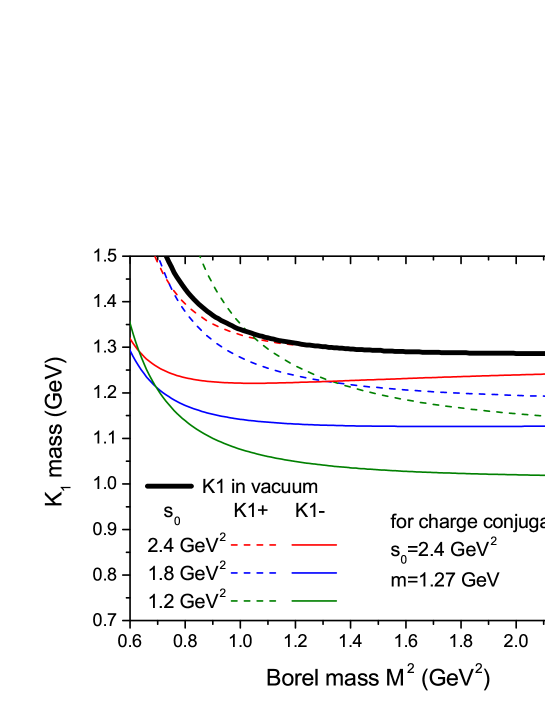
Figure 2: The Borel curve for $K_{1}$ mass from $\Pi_{1}$ sum rule at nuclear matter density.

III.3.2 In-medium width

So far, we have approximated the spectral function as the sum of a delta function for the ground state and a step function for excited states. However, in-medium spectral function would have more complicated structure, and the medium modification of the OPE side is reflected as a combination of the mass and width changes in QCD sum rules (see e.g. the 3rd reference in  Klingl:1997kf ). In order to investigate this possibility, we replace the delta function by the Breit-Wigner form,

$$\delta(s-m_{\pm}^{2})\rightarrow\frac{1}{\pi}\frac{\sqrt{s}~{}\Gamma_{\pm}}{(s-m_{\pm}^{2})^{2}+s\Gamma_{\pm}^{2}},$$ (31)

where $\Gamma_{\pm}$ is the width of $K_{1}^{\pm}$. We will allow the width to change by $\Gamma_{\pm}=\Gamma_{K_{1}}+\Gamma^{\prime}_{\pm}\rho$ in nuclear matter at low density. We expand $F_{\pm}$, $\Gamma_{\pm}$ and $s_{0}^{\pm}$ up to the linear order in $\rho$, while keeping $m_{\mp}(\rho)$ without expansion. This is to probe the maximum width change associated with the change in the OPE Leupold:1997dg . Eq. (26) and Eq. (27) are then modified as

$$\mathcal{F}(M^{2})F_{\pm}^{\prime}+\mathcal{W}(M^{2})\Gamma^{\prime}_{\pm}+\mathcal{S}(M^{2}){s^{\prime}}_{0}^{\pm}=\mathcal{C}_{\pm}(M^{2}),$$

where $\Gamma^{\prime}_{\pm}$ is considered as variables instead of $m^{\prime}_{\pm}$, and the terms proportional to $m^{\prime}_{\pm}$ are moved into $\mathcal{C}_{\pm}(M^{2})$ as

$$\mathcal{F}(M^{2})=-\frac{1}{\pi}\int_{0}^{\infty}\frac{s^{3/2}\Gamma_{K_{1}}}{(s-m_{K_{1}}^{2})^{2}+s\Gamma_{K_{1}}^{2}}e^{-s/M^{2}}ds,~{}~{}~{}~{}~{}~{}$$

$$\mathcal{W}(M^{2})=-\frac{F_{K_{1}}}{\pi}\int_{0}^{\infty}\frac{s^{3/2}\Gamma_{K_{1}}}{(s-m_{K_{1}}^{2})^{2}+s\Gamma_{K_{1}}^{2}}~{}~{}~{}~{}~{}~{}~{}~{}~{}~{}~{}~{}~{}~{}$$

$$\times\bigg{(}1-\frac{2s\Gamma_{K_{1}}^{2}}{(s-m_{K_{1}}^{2})^{2}+s\Gamma_{K_{1}}^{2}}\bigg{)}e^{-s/M^{2}}ds,$$

$$\mathcal{S}(M^{2})=S(M^{2}),~{}~{}~{}~{}~{}~{}~{}~{}~{}~{}~{}~{}~{}~{}~{}~{}~{}~{}~{}~{}~{}~{}~{}~{}~{}~{}~{}~{}~{}~{}~{}~{}~{}~{}~{}~{}~{}~{}~{}~{}~{}~{}~{}~{}~{}~{}$$

$$\mathcal{C}_{\pm}(M^{2})=-m_{s}\langle\bar{u}u\rangle_{N}+\frac{\alpha_{s}}{12\pi}\langle G^{2}\rangle_{N}~{}~{}~{}~{}~{}~{}~{}~{}~{}~{}~{}~{}~{}~{}~{}~{}~{}~{}~{}~{}~{}~{}~{}~{}$$

$$+\frac{m_{N}}{2}(A_{2}^{u}+A_{2}^{s})\pm\frac{m_{K_{1}}}{3}(A_{1}^{u}-A_{1}^{s})~{}~{}~{}~{}~{}~{}~{}~{}~{}~{}~{}~{}~{}~{}~{}$$

$$+\frac{32\pi\alpha_{s}}{9M^{2}}\bigg{\{}\langle\bar{u}u\rangle_{N}\langle\bar{s}s\rangle_{0}+\langle\bar{u}u\rangle_{0}\langle\bar{s}s\rangle_{N}$$

$$+\frac{2}{9}(\langle\bar{u}u\rangle_{N}\langle\bar{u}u\rangle_{0}+\langle\bar{s}s\rangle_{N}\langle\bar{s}s\rangle_{0})\bigg{\}}$$

$$-\frac{5}{6M^{2}}m_{N}^{3}(A_{4}^{u}+A_{4}^{s})\mp\frac{2m_{K_{1}}m_{N}^{2}}{3M^{2}}(A_{3}^{u}-A_{3}^{s})~{}~{}~{}~{}~{}~{}$$

$$+m^{\prime}_{\pm}\bigg{\{}\frac{F_{K_{1}}}{2\pi m_{K_{1}}}\int_{0}^{\infty}\frac{s^{3/2}\Gamma_{K_{1}}e^{-s/M^{2}}}{(s-m_{K_{1}}^{2})^{2}+s\Gamma_{K_{1}}^{2}}~{}~{}~{}~{}~{}~{}~{}~{}~{}~{}~{}$$

$$\times\bigg{(}1-\frac{8m_{K_{1}}^{2}(s-m_{K_{1}}^{2})}{(s-m_{K_{1}}^{2})^{2}+s\Gamma_{K_{1}}^{2}}\bigg{)}ds\bigg{\}}~{}~{}~{}~{}~{}~{}~{}$$

$$+m_{\mp}{{}^{\prime}}\bigg{\{}-\frac{F_{K_{1}}}{2\pi m_{K_{1}}}\int_{0}^{\infty}\frac{s^{3/2}\Gamma_{K_{1}}e^{-s/M^{2}}}{(s-m_{K_{1}}^{2})^{2}+s\Gamma_{K_{1}}^{2}}ds\bigg{\}}~{}~{}$$

$$+{s^{\prime}}_{0}^{\mp}\bigg{\{}\frac{1}{2}\bigg{(}-1+\frac{m_{K_{1}}}{\sqrt{s_{0}}}\bigg{)}(B_{0}s_{0}-B_{2})e^{-s_{0}/M^{2}}\bigg{\}}.~{}~{}$$

Defining the function $V(F^{\prime}_{\pm},\Gamma^{\prime}_{\pm},{s^{\prime}}_{0}^{\pm})$ similarly as before, the differential equations

$$\frac{\partial V_{\pm}}{\partial F^{\prime}_{\pm}}=\frac{\partial V_{\pm}}{\partial\Gamma^{\prime}_{\pm}}=\frac{\partial V_{\pm}}{\partial{s^{\prime}}_{0}^{\pm}}=0,$$

are expressed as

$$F^{\prime}_{\pm}\int dM^{2}\mathcal{F}^{2}(M^{2})+\Gamma^{\prime}_{\pm}\int dM^{2}\mathcal{F}(M^{2})\mathcal{M}(M^{2})+{s^{\prime}}_{0}^{\pm}\int dM^{2}\mathcal{F}(M^{2})\mathcal{S}(M^{2}) = \int dM^{2}\mathcal{F}(M^{2})\mathcal{C}_{\pm}(M^{2}),$$

$$F^{\prime}_{\pm}\int dM^{2}\mathcal{F}(M^{2})\mathcal{M}(M^{2})+\Gamma^{\prime}_{\pm}\int dM^{2}\mathcal{M}^{2}(M^{2})+{s^{\prime}}_{0}^{\pm}\int dM^{2}M(M^{2})S(M^{2}) = \int dM^{2}M(M^{2})\mathcal{C}_{\pm}(M^{2}),$$

$$F^{\prime}_{\pm}\int dM^{2}\mathcal{F}(M^{2})\mathcal{S}(M^{2})+\Gamma^{\prime}_{\pm}\int dM^{2}\mathcal{M}(M^{2})\mathcal{S}(M^{2})+{s^{\prime}}_{0}^{\pm}\int dM^{2}\mathcal{S}^{2}(M^{2}) = \int dM^{2}\mathcal{S}(M^{2})\mathcal{C}_{\pm}(M^{2}).$$ (33)

We find that Eq. (33) has only a weak dependence on the vacuum width $\Gamma_{K_{1}}$, so that we take $\Gamma_{K_{1}}=0$ in solving the coupled equations since the input parameters $F_{K_{1}}$ and $s_{0}$ were obtained in this limit. Figure 3 shows the constraints on the mass modification, $\delta m_{\pm}(\rho)=m_{\pm}(\rho)-m_{K_{1}}$ and the width modification $\delta\Gamma_{\pm}(\rho)=\Gamma^{\prime}_{\pm}\rho$ obtained from Eq. (33). As for $K_{1}^{-}$, the maximum change of the width is +275 MeV, while +38 MeV for $K_{1}^{+}$. The decay of the $K_{1}$ is dominated by $K\rho$ ($42\pm 6$%) in vacuum. Therefore, keeping the $K_{1}$ mass the same, if the mass of $K^{-}$ ($K^{+}$) decreases (remains the same) in the medium, the phase space for the corresponding $K\rho$ decay for $K_{1}^{-}$ ($K_{1}^{+}$) will increase (remain the same), which provides a possible physical mechanism for their asymmetric width change in medium.

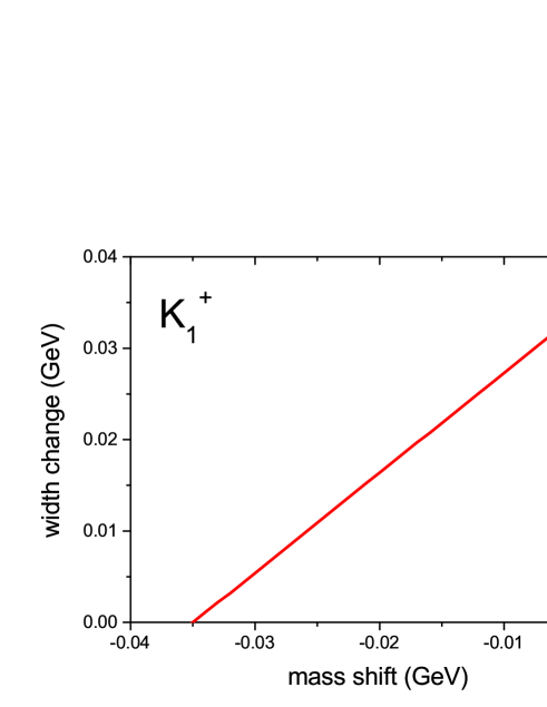
Figure 3: The constraints on the mass shift and the width change of $K_{1}^{\pm}$ in the nuclear matter

IV Summary and discussions

In this paper, we have carried out QCD sum rule analyses for the open strange meson $K_{1}$ in the vacuum and in the medium. We first show that the experimental mass of $K_{1}(1270)$ in the vacuum is well reproduced by the QCD condensates with a proper choice of the continuum threshold and the Borel window. In nuclear matter, $K_{1}^{-}$ and $K_{1}^{+}$ become non-degenerate due to the breaking of the charge conjugation invariance. By extracting the ground state of each charge state from the polarization functions and by formulating coupled QCD sum rules in nuclear matter, we obtained a relation between the in-medium mass and width of $K_{1}^{\pm}$ through the density dependence of the scalar and twist-two condensates. In particular, the upper limit of the mass shifts for $K_{1}^{-}$ and $K_{1}^{+}$ without width modifications are -249 MeV and -35 MeV, respectively, which indicates that $K_{1}^{-}(s\bar{u})$ ($K_{1}^{-}(\bar{s}u)$) feels attraction (repulsion) in nuclear matter. Once the change of the widths is allowed, however, those mass shifts get smaller. Furthermore, the $K_{1}(1270)$ and $K_{1}(1400)$ are the analogues of $a_{1}$ and $b_{1}$ mesons and can be analyzed through the axial vector as well as tensor currents Jeong:2018exh . A more detailed discussion on how the these currents couple to $K_{1}(1270)$ and $K_{1}(1400)$ in the medium together with their respective mass changes are an important topic for future investigations.

Experimentally $K_{1}^{-}$ is known to be produced through $K^{-}$-nucleon reactions Gavillet:1978rj ; Daum:1981hb , so that the modification of $K_{1}^{-}$ in nuclei would be best searched through the $K^{-}$ reaction on various nuclear targets. Such experimental possibility may be provided by the kaon beam at J-PARC with the energy up to 2.0 GeV. Maximum $\sqrt{s}$ of a kaon and a nucleon is 2.23 GeV ignoring the fermi motion, and is as large as 2.48 GeV including the fermi motion. Those numbers are close to the threshold value of the $K_{1}^{-}$ production which is around 2.2 GeV. The measurement of hadronic decays ($K_{1}\rightarrow K~{}\rho$ and $K_{1}\rightarrow K^{*}\pi$) as well as the measurement of the excitation function would be possible probes to detect the spectral shift of $K_{1}^{-}$. Furthermore, similar experiments for the $K^{*}$ (the chiral partner of $K_{1}$) will give model-independent estimate of the chiral order parameter in the medium, and hence provide crucial hints to the partial restoration of chiral symmetry in nuclear medium.

References

- (1) S. Weinberg, Phys. Rev. Lett. 18, 507 (1967).
- (2) M. A. Shifman, A. I. Vainshtein and V. I. Zakharov, Nucl. Phys. B 147, 385 (1979); M. A. Shifman, A. I. Vainshtein and V. I. Zakharov, Nucl. Phys. B 147, 448 (1979).
- (3) T. Hatsuda and T. Kunihiro, Phys. Rev. Lett. 55, 158 (1985).
- (4) G. E. Brown and M. Rho, Phys. Rev. Lett. 66, 2720 (1991).
- (5) T. Hatsuda and S. H. Lee, Phys. Rev. C 46, no. 1, R34 (1992).
- (6) F. Klingl, N. Kaiser and W. Weise, Nucl. Phys. A 624, 527 (1997). R. Rapp and J. Wambach, Adv. Nucl. Phys. 25, 1 (2000). S. Leupold, V. Metag and U. Mosel, Int. J. Mod. Phys. E 19, 147 (2010). P. Gubler and W. Weise, Nucl. Phys. A 954, 125 (2016).
- (7) K. Suzuki et al., Phys. Rev. Lett. 92, 072302 (2004). P. Kienle and T. Yamazaki, Prog. Part. Nucl. Phys. 52, 85 (2004).
- (8) E. E. Kolomeitsev, N. Kaiser and W. Weise, Phys. Rev. Lett. 90, 092501 (2003). D. Jido, T. Hatsuda and T. Kunihiro, Phys. Lett. B 670, 109 (2008).
- (9) R. S. Hayano and T. Hatsuda, Rev. Mod. Phys. 82, 2949 (2010).
- (10) M. Naruki et al., Phys. Rev. Lett. 96, 092301 (2006).
- (11) R. Muto et al. [KEK-PS-E325 Collaboration], Phys. Rev. Lett. 98, 042501 (2007).
- (12) M. Ichikawa et al., arXiv:1806.10671 [physics.ins-det].
- (13) D. Trnka et al. [CBELSA/TAPS Collaboration], Phys. Rev. Lett. 94, 192303 (2005).
- (14) P. Gubler, T. Kunihiro and S. H. Lee, Phys. Lett. B 767, 336 (2017).
- (15) A. K. Dutt-Mazumder, R. Hofmann and M. Pospelov, Phys. Rev. C 63, 015204 (2001).
- (16) R. Thomas, S. Zschocke and B. Kampfer, Phys. Rev. Lett. 95, 232301 (2005).
- (17) S. Leupold, V. Metag and U. Mosel, Int. J. Mod. Phys. E 19, 147 (2010).
- (18) V. Metag, M. Nanova and E. Y. Paryev, Prog. Part. Nucl. Phys. 97, 199 (2017).
- (19) R. Dickson et al. [CLAS Collaboration], Phys. Rev. C 93, 065202 (2016).
- (20) S. H. Lee and S. Cho, Int. J. Mod. Phys. E 22, 1330008 (2013).
- (21) M. Suzuki, Phys. Rev. D 47, 1252 (1993).
- (22) T. Hatsuda, arXiv:nucl-th/9702002.
- (23) D. Jido, N. Kodama and M. Oka, Phys. Rev. D 54, 4532 (1996).
- (24) K. Suzuki, P. Gubler and M. Oka, Phys. Rev. C 93, no. 4, 045209 (2016).
- (25) Y. Kondo, O. Morimatsu and T. Nishikawa, Nucl. Phys. A 764, 303 (2006).
- (26) R. J. Furnstahl, D. K. Griegel and T. D. Cohen, Phys. Rev. C 46, 1507 (1992).
- (27) M. Tanabashi et al. [Particle Data Group], Phys. Rev. D 98, no. 3, 030001 (2018).
- (28) C. A. Dominguez, L. A. Hernandez and K. Schilcher, JHEP 1507, 110 (2015).
- (29) V. A. Novikov, M. A. Shifman, A. I. Vainshtein and V. I. Zakharov, Nucl. Phys. B 249, 445 (1985) [Yad. Fiz. 41, 1063 (1985)].
- (30) S. H. Lee, Phys. Rev. D 40, 2484 (1989).
- (31) T. Hilger, B. Kampfer and S. Leupold, Phys. Rev. C 84, 045202 (2011).
- (32) T. Buchheim, T. Hilger and B. Kampfer, Phys. Rev. C 91, 015205 (2015).
- (33) L. J. Reinders, S. Yazaki and H. R. Rubinstein, Nucl. Phys. B 196, 125 (1982).
- (34) B. Friman, S. H. Lee and H. C. Kim, Nucl. Phys. A 653, 91 (1999).
- (35) A. D. Martin, W. J. Stirling, R. S. Thorne and G. Watt, Eur. Phys. J. C 63, 189 (2009).
- (36) A. D. Martin, Nucl. Phys. B 179, 33 (1981). J. S. Hyslop, R. A. Arndt, L. D. Roper and R. L. Workman, Phys. Rev. D 46, 961 (1992). L. Tolos, C. Garcia-Recio, R. Molina, J. Nieves, E. Oset, A. Ramos and L. L. Salcedo, PoS ConfinementX , 015 (2012).
- (37) S. Leupold, W. Peters and U. Mosel, Nucl. Phys. A 628, 311 (1998).
- (38) K. S. Jeong, S. H. Lee and Y. Oh, JHEP 1808, 179 (2018).
- (39) P. Gavillet et al. [Amsterdam-CERN-Nijmegen-Oxford Collaboration], Phys. Lett. B 76, 517 (1978).
- (40) C. Daum et al. [ACCMOR Collaboration], Nucl. Phys. B 187, 1 (1981).
- (41) P. Morath, W. Weise and S. H. Lee, Prepared for 17th Autumn School: QCD: Perturbative or Nonperturbative? (AUTUMN 99), Lisbon, Portugal, 29 Sep - 4 Oct 1999; Ph. D. thesis of P. Morath 2001 Schwere Quarks in dichter Materie, Technische Universität München.
- (42) Y. Kondo, O. Morimatsu and Y. Nishino, Phys. Rev. C 53, 1927 (1996).