Dynamo Action in the Steeply Decaying Conductivity Region of Jupiter-like Dynamo Models

Abstract

The Juno mission is delivering spectacular data of Jupiter’s magnetic field, while the gravity measurements finally allow constraining the depth of the winds observed at cloud level. However, to which degree the zonal winds contribute to the planet’s dynamo action remains an open question. Here we explore numerical dynamo simulations that include an Jupiter-like electrical conductivity profile and successfully model the planet’s large scale field. We concentrate on analyzing the dynamo action in the Steeply Decaying Conductivity Region (SDCR) where the high conductivity in the metallic Hydrogen region drops to the much lower values caused by ionization effects in the very outer envelope of the planet. Our simulations show that the dynamo action in the SDCR is strongly ruled by diffusive effects and therefore quasi stationary. The locally induced magnetic field is dominated by the horizontal toroidal field, while the locally induced currents flow mainly in the latitudinal direction. The simple dynamics can be exploited to yield estimates of surprisingly high quality for both the induced field and the electric currents in the SDCR. These could be potentially be exploited to predict the dynamo action of the zonal winds in Jupiter’s SDCR but also in other planets.

1 Introduction

Jupiter’s electrical conductivity profile likely has a strong impact on the interior dynamics. Ab initio calculations (French et al., 2012) show that the conductivity first increases with depth at a super-exponential rate due to hydrogen ionization. At about $0.90\,r_{J}$, however, hydrogen undergoes a phase transition from the molecular to a metallic state and the conductivity increases much more smoothly with depth (see fig. 1).

It is commonly thought, that Jupiter’s dynamo operates in the deeper metallic region, while the fierce zonal wind system observed on the surface is limited to the molecular outer shell. However, recent numerical simulations show that the interaction between both regions yields complex and interesting dynamics. For example, the zonal winds may drive a secondary dynamo where they reach down to significant enough electrical conductivities. Possible spotting feature of such a process would are banded structures and large scale spots at low to mid latitudes (Gastine et al., 2014b; Duarte et al., 2018), very similar to those observed recently by NASA’s Juno mission (Connerney et al., 2018).

One of the main Juno objectives is to determine the depth of the fierce zonal winds observed on the planet’s surface. Since the winds dynamics is tied to density variations (Kaspi et al., 2018), the gravity signal can help to constrain their depth. A recent analysis by Kaspi et al. (2018), based on the equatorially antisymmetric gravity moments $J_{3}$ to $J_{9}$ measured by Juno mission, concludes that the wind speed must be significantly reduced at a about $3000\,$km depth, which corresponds to about $0.96\,r_{J}$.

Older estimates of the wind depth rely on magnetic effects. Liu et al. (2008) concluded that the Ohmic heat produced by the zonal wind induced electric currents would exceed the heating emitted from the planets interior, should the winds reach deeper than $0.96\,r_{J}$ with undiminished speed. Ridley and Holme (2016) argue that the variation of the large scale field deduced from pre-Juno measurements is so small that the zonal winds cannot contribute. The winds are thus unlikely to penetrate deeper than about $0.96\,r_{J}$ where the magnetic Reynolds number exceeds unity (Cao and Stevenson, 2017).

Another hint on the depth of the zonal winds comes from the width of the prograde equatorial jet. Numerical simulations suggest that it is determined by the depth of the spherical shell the winds live in. The observed with is consistent with a lower boundary at about $0.95\,r_{J}$ (Gastine et al., 2014a).

Classically, the magnetic Reynolds number attempts to quantify the ratio of magnetic induction to Ohmic dissipation in the dynamo equation

$$\frac{\partial\mbox{$\mathbf{B}$}}{\partial t}=\nabla\times\left(\mbox{$\mathbf{U}$}\times\mbox{$\mathbf{B}$}\right)-\nabla\times\left(\lambda\nabla\times\mbox{$\mathbf{B}$}\right)\;\;,$$ (1)

where $\lambda=1/(\mu\sigma)$ is the magnetic diffusivity and $\sigma$ the electrical conductivity. The Ohmic dissipation term can be separated into two parts,

$$\nabla\times\left(\lambda\nabla\times\mbox{$\mathbf{B}$}\right)=-\lambda\,\nabla^{2}\mbox{$\mathbf{B}$}+\frac{\lambda}{d_{\lambda}}\,\hat{\mathbf{r}}\times\left(\nabla\times\mbox{$\mathbf{B}$}\right)\;\;,$$ (2)

where the second depends on the magnetic diffusivity scale height $d_{\lambda}=\lambda/(\partial\lambda/\partial r)$. The classical magnetic Reynolds number

$$\mbox{Rm}=\frac{\mbox{U}d}{\lambda}\;\;,$$ (3)

ignores the second term that would dominate where $\sigma$ decreases rapidly in Jupiter’s outer envelope. Here $d$ is a reference length scale and U typical flow velocity and $d$ a reference length scale, Liu et al. (2008) argue that the appropriate definition for this particular Steeply Decaying Conductivity Region (SDCR) should include the diffusivity scale height:

$$\mbox{Rm}^{(1)}=\frac{\mbox{U}d_{\lambda}}{\lambda}\;\;.$$ (4)

In Jupiter, the SDCR roughly coincides with the molecular outer envelope where ionization effects determine the electrical conductivity.

For a selfconsistent dynamo to operate, the overall field production has to overcome diffusion. The mean global magnetic Reynolds number for the whole dynamo region should thus exceed a critical value $\mbox{Rm}_{c}=1$. However, since the definition of Rm ignores many complexities of the dynamo process, the exact critical value is always higher and can only be determined by experiments. Christensen and Aubert (2006) explore a suite of Boussinesq dynamo simulations with rigid flow boundary conditions and constant conductivity and find selfconsistent dynamo action when the rms magnetic Reynolds number exceeds $\mbox{Rm}_{c}\approx 50$.

The radius $r_{D}$ where the magnetic Reynolds number exceeds $\mbox{Rm}_{c}$ indicates the ’top of the dynamo region’ that could potentially host selfconsistent dynamo action. Gastine et al. (2014b) and Duarte et al. (2018) use $\mbox{Rm}_{c}\approx 50$ in combination with the classical Rm definition (3) and show that Jupiter-like magnetic field are found when $r_{D}>0.9\,r_{J}$. Extrapolating their findings to Jupiter conditions suggest $r_{D}\approx 0.95\,r_{J}$.

There are several reasons, however, why these consideration are problematic. For one, self-consistent dynamo action and the related critical magnetic Reynolds number are defined in a mean sense for the ’whole’ dynamo region. The local dynamo mechanism at any given radius, however, also includes the modification of the field produced elsewhere. Another fundamental problem is that the magnetic Reynolds number actually ceases to provide a decent proxy for the ratio of induction to diffusion in the SDCR. The reason is that the magnetic field approaches a diffusion-less potential field as the conductivity decays.

A more useful definition of the ’top of the dynamo region’ would be the depth where the locally induced field becomes a significant fraction of the total field. Cao and Stevenson (2017) suggest that Rm⁽¹⁾ takes on a different role in the SDCR  and may allow to quantify the ratio of locally induced field $\hat{\mbox{$\mathbf{B}$}}$ to the background field $\tilde{\mbox{$\mathbf{B}$}}$. Using a simplified mean field dynamo model, they conclude that $\hat{\mbox{$\mathbf{B}$}}$ could reach $1\,$% of the background field in the SDCR.

The different estimates put the depth of the zonal winds in the SDCR  beyond $0.9\,r_{J}$. In this article we closely analyze the dynamo action in the SDCR for two different numerical dynamo simulations that both yield Jupiter-like large scale magnetic fields. After presenting the numerical dynamo model in sect. 2, we analyze the simulation results in sect. 3. Sect. 4 is then devoted to deriving estimates for the locally induced electric current and field that could be applied to planets. The paper closes with a discussion and conclusions in sect. 5.

2 Numerical Dynamo Model

2.1 Fundamental Equations

The numerical simulations were performed with the MHD-code MagIC that is freely available on GitHub (https://github.com/magic-sph/magic). MagIC solves for small disturbances around an adiabatic, hydrostatic background state that only depends on radius. Using the anelastic approximation for the Navier-Stokes equation allows incorporating the background density gradient $\widetilde{\rho}(r)$ while filtering out fast sound waves.

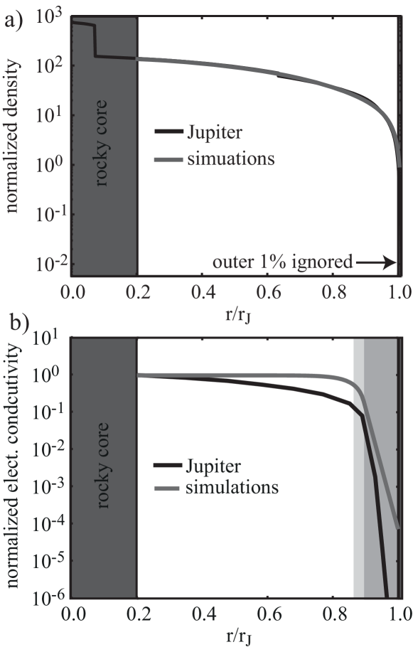
Figure 1: Comparison of the Jupiter interior model by (French et al., 2012) (black lines) with the model used for the numerical simulations (grey). Panel a) and b) show the normalized background density and electrical conductivity, respectively. Dark grey background colors mark the outer $1$% that have been neglected in the simulations and the assumed solid inner core. Medium gray highlights the Steeply Decaying Conductivity Region (SDCR) of the model conductivity profile while Light grey marks the low conductivity region where the conductivity is smaller than $50$% of the inner boundary reference value.

The background state is based on the Jupiter model by French et al. (2012) and Nettelmann et al. (2012), which uses ab initio simulations to determine the equation of states for Hydrogen and Helium and to calculate the transport properties. Fig. 1 shows the normalized density profile $\widetilde{\rho}$ and electrical conductivity profile $\widetilde{\sigma}$ along with the profiles that have been assumed in the simulations. The transition to a metallic hydrogen state takes place at about $0.9\,r_{J}$. Jupiter’s Steeply Decaying Conductivity Region (SDCR) occupies the outer $10\,$% in radius and is highlighted by a medium gray background color. Here, the conductivity decays increasingly rapidly with radius, eventually reaching super-exponential rates.

The numerical models disregard the outer one percent in radius where the density gradient in steepest and thus very difficult to resolve numerically. The conductivity profile used in the simulations is a combination of a polynomial branch,

$$\sigma=\sigma_{i}+(\sigma_{m}-\sigma_{i})\left(\frac{r-r_{i}}{r_{m}-r_{i}}\right)^{a}\;\;\mbox{for}\;\;r<r_{m}$$ (5)

and an exponential branch,

$$\sigma=\sigma_{m}\exp\left(\frac{r-r_{m}}{r_{m}-r_{i}}\frac{\sigma_{m}-\sigma_{i}}{\sigma_{m}}\right)\;\;\mbox{for}\;\;r\geq r_{m}\;\;.$$ (6)

Here $\sigma_{i}$ is the reference conductivity at the bottom boundary $r_{i}$, $a$ is the exponential decay rate, and $r_{m}$ is the transition radius where both branches meet with $\sigma(r_{m})=\sigma_{m}$.

While the ab initio simulations suggest that the conductivity already slowly decreases in the metallic region, we assume a constant value here. This keeps the magnetic Reynolds number at values that allow for dynamo action throughout this region (Duarte et al., 2018). In the molecular region, our model profile decreases slower than suggested by French et al. (2012) to ease the numerical calculations. The total conductivity contrasts is about four orders of magnitude and we identify the SDCR with the exponential branch (6).

The mathematical formulation of the problem has been extensively discussed elsewhere (Jones et al., 2011; Wicht et al., 2018). Detailed information can also be found in the online MagIC manual (http://magic-sph.github.io/). Here we only briefly introduce the essential equations.

MagIC solves the non-dimensional Navier-Stokes equation,

$$\mbox{E}\,\widetilde{\rho}\;\frac{d\mbox{$\mathbf{U}$}}{dt} = -\widetilde{\rho}\;\nabla\left(\frac{p}{\widetilde{\rho}}\right)+2\widetilde{\rho}\;\mbox{$\mathbf{U}$}\times\hat{\mathbf{z}}-\frac{\mbox{Ra}^{\prime}\,\mbox{E}}{\mbox{Pr}\,\mbox{Di}}\;\widetilde{\rho}\;\frac{\partial\widetilde{T}}{\partial r}\;S\,\hat{\mathbf{r}}$$

$$+\frac{1}{\mbox{Pm}_{i}}(\nabla\times\mbox{B})\times\mbox{B}+\mbox{E}\,\widetilde{\rho}\;{\mathbf{F}}_{v}\;\;\textrm{,}$$

the heat equation

$$\widetilde{\rho}\,\widetilde{T}\,\frac{ds}{dt}=\frac{1}{\mbox{Pr}}\nabla\cdot\left(\widetilde{\rho}\widetilde{T}\,\nabla s\right)+\frac{\mbox{Pr}\,\mbox{Di}}{\mbox{Ra}^{\prime}}\left(q_{\nu}+\frac{1}{\mbox{Pm}_{i}^{2}\,\mbox{E}}q_{J}\right)+q_{s}\;\;,$$ (8)

the induction equation

$$\frac{\partial\mbox{$\mathbf{B}$}}{\partial t}=\nabla\times(\mbox{$\mathbf{U}$}\times\mbox{$\mathbf{B}$})-\frac{1}{\mbox{Pm}_{i}}\nabla\times(\widetilde{\lambda}\nabla\times\mbox{$\mathbf{B}$})\;\;,$$ (9)

the continuity equation

$$\nabla\cdot(\widetilde{\rho}\mbox{$\mathbf{U}$})=0\;\;,$$ (10)

and the solonoidal condition for the magnetic field

$$\nabla\cdot\mbox{$\mathbf{B}$}=0\;\;.$$ (11)

Here $p$ is a modified pressure that also includes centrifugal effects and accounts for disturbances in the gravity potential. Buoyancy variations are formulated in terms of the specific entropy $s$. Using the gradient of the normalized background temperature $\widetilde{T}$ in the buoyancy term guarantees a consistent background gravity (Wicht et al., 2018). The three volumetric heating terms in eqn. (8) are viscous heating $q_{\nu}$, Joule or Ohmic heating $q_{J}$, and secular cooling $q_{s}$ (Wicht et al., 2018).

The dimensionless parameters ruling the system are the Ekman number

$$\mbox{E}=\frac{\nu}{\Omega d^{2}}\;\;\textrm{,}$$ (12)

the modified Rayleigh number

$$\mbox{Ra}^{\prime}=\frac{\alpha_{o}\widetilde{g}_{o}d^{3}\widetilde{T}_{o}}{\nu\kappa_{S}}\frac{s_{s}}{c_{p}}=\mbox{Ra}\frac{S_{s}}{c_{p}}\;\;\textrm{,}$$ (13)

the Prandtl number

$$\mbox{Pr}=\frac{\nu}{\kappa_{S}}\;\;\textrm{,}$$ (14)

and the inner boundary magnetic Prandtl number

$$\mbox{Pm}_{i}=\frac{\nu}{\lambda_{i}}\;\;\textrm{.}$$ (15)

Here $\nu$ is the (homogeneous) kinematic viscosity, $\Omega$ the rotation rate, $\alpha_{o}$ the outer boundary thermal expansivity , $\widetilde{g}_{o}$ the outer-boundary gravity, $d=r_{o}-r_{i}$ the shell thickness, $\kappa_{S}$ the entropy diffusivity, $s_{s}$ the entropy scale, $c_{p}$ the heat capacity, $\lambda_{i}=1/(\mu_{o}\sigma_{i})$ the inner boundary magnetic diffusivity, $\hat{\mathbf{r}}$ the radial unit vector, and $\hat{\mathbf{z}}$ the unit vector in the direction of the rotation axis. The aspect ratio, another dimensionless parameter, has been fixed to $r_{i}/r_{o}=0.2$.

The modified Rayleigh number $\mbox{Ra}^{\prime}$ is the product of the classical Rayleigh number Ra and the dimensionless entropy scale $s_{s}/c_{p}$. The dissipation number

$$\mbox{Di}=\frac{d}{\widetilde{T}_{o}}\left(\frac{\partial\widetilde{T}}{\partial r}\right)_{r_{o}}=\frac{d\alpha_{o}\widetilde{g}_{o}}{c_{p}}$$ (16)

is defined by the background temperature $\widetilde{T}$.

The equations have been non-dimensionalize by using the imposed entropy difference as entropy scale $s_{s}$, the difference between outer radius $r_{o}$ and inner radius $r_{i}$ as a length scale $d=r_{o}-r_{i}$, the viscous diffusion time $d^{2}/\nu$ as a time scale, and $\sqrt{\Omega\mu_{0}\lambda_{i}\widetilde{\rho}_{o}}$ as a magnetic scale, where $\tilde{\rho}_{o}$ is the outer boundary reference density. We use entropy rather than temperate diffusion in the heat equation, which considerably simplifies the system (Braginsky and Roberts, 1995). In the above formulation, the dimensionless profiles $\widetilde{\rho}$, $\widetilde{T}$ and $\widetilde{\lambda}$ carry the information on the radial dependence of the background state.

2.2 Poloidal/Toroidal Decomposition

We use the common representation of the divergence free magnetic field by a poloidal and a toroidal contribution,

$$\mbox{$\mathbf{B}$}=\mbox{$\mathbf{B}$}^{(P)}+\mbox{$\mathbf{B}$}^{(T)}=\nabla\times\nabla\times\hat{\mathbf{r}}\;b^{(P)}+\nabla\times\hat{\mathbf{r}}\;b^{(T)}\;\;,$$ (17)

where $b^{(P)}$ is the poloidal and $b^{(T)}$ the toroidal scalar potential. The respective decomposition for the electric current density $\mathbf{j}$ reads

$$\mbox{$\mathbf{j}$}=\mbox{$\mathbf{j}$}^{(P)}+\mbox{$\mathbf{j}$}^{(T)}=\nabla\times\nabla\times\hat{\mathbf{r}}\;i^{(P)}+\nabla\times\hat{\mathbf{r}}\;i^{(T)}\;\;,$$ (18)

where $i^{(P)}$ denotes the poloidal and $i^{(T)}$ the toroidal potential.

Simple vector calculus yields

$$\mbox{$\mathbf{j}$}=-\nabla_{H}^{2}\,i^{(P)}\;\hat{\mathbf{r}}+\nabla_{H}\frac{\partial}{\partial r}\,i^{(P)}+\nabla\times\,\hat{\mathbf{r}}\;i^{(P)}\;\;,$$ (19)

where $\nabla_{H}$ is the horizontal component of the nabla operator. The toroidal contribution obviously has no radial component. Radial derivatives appear only in the horizontal poloidal current density, which therefore dominates in the SDCR, as we will show below.

Ampere’s law, $\nabla\times\mbox{$\mathbf{B}$}=\mu\mbox{$\mathbf{j}$}$, connects the poloidal (toroidal) magnetic field to the toroidal (poloidal) current density. Its radial component establishes a connection to the toroidal field potential:

$$\mu j_{r}=-\mu\nabla_{H}^{2}\,i^{(P)}\;\hat{\mathbf{r}}=\hat{\mathbf{r}}\cdot(\nabla\times\mbox{$\mathbf{B}$})=-\nabla_{H}^{2}b^{(T)}\;\hat{\mathbf{r}}\;\;.$$ (20)

The toroidal field at a given radius is thus determined by the radial currents flowing through the respective radial shell.

2.3 Selected Simulations

We concentrate on closely analyzing two quite different dynamo simulations that both reproduce Jupiter’s large scale field (Duarte et al., 2018). Model G14 has been introduced by Gastine et al. (2014b) while model D18 is listed as model number 20 in Duarte et al. (2018); tab. 1 compares their parameters. Both dynamos share the background pressure, temperature, density, and electrical conductivity models (see fig. 1), use stress-free outer but rigid inner boundary condition, employ constant entropy boundary conditions, and are driven by heat coming in through the lower boundary. Model D18 uses a larger Ekman and larger magnetic Prandtl number. The Prandtl number is one in G14 but only $0.1$ in D18. A consequence is the the smaller scale field in D18 Duarte et al. (2018).

Fig. 2 compares the radial surface field for the two snapshots we will continue to analyze throughout the paper with the recent Jupiter field model JRM09 by Connerney et al. (2018). The non-dimensional fields in the computer models have been rescaled to reflect the Jovian parameters using the methods explained in Gastine et al. (2014b) and Duarte et al. (2018).

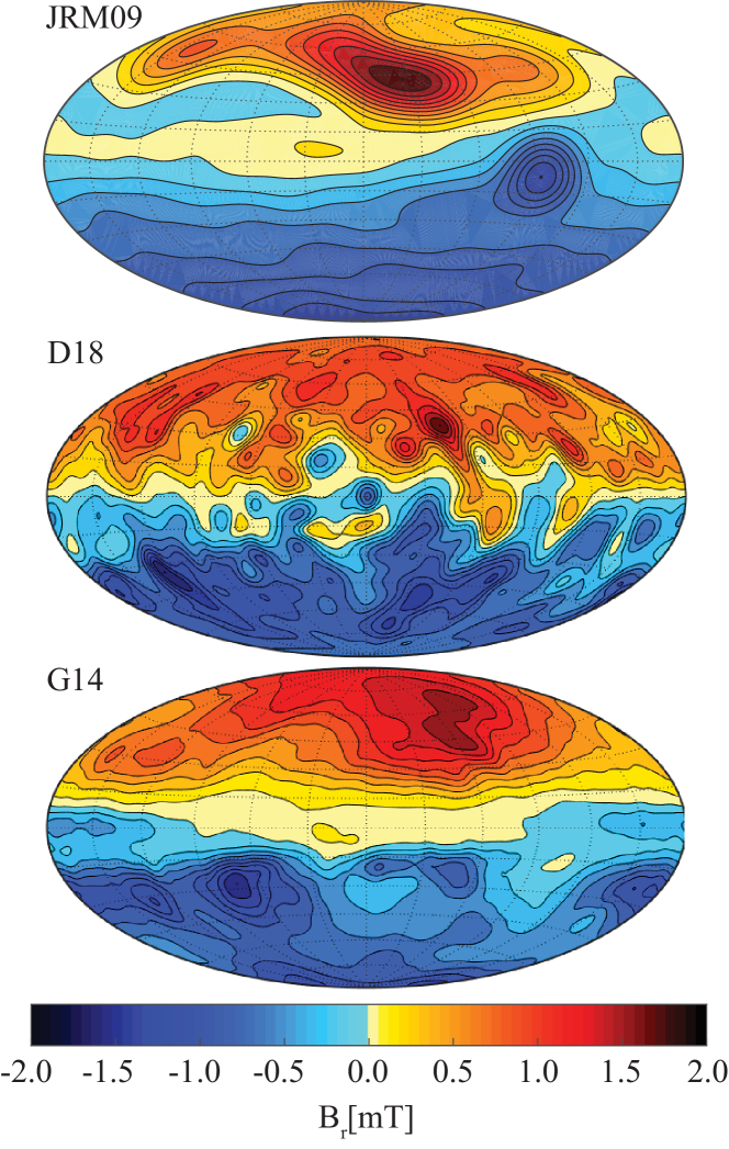
Figure 2: Comparison of the surface radial magnetic field in the recent Jupiter field model JRM09 (Connerney et al., 2018) with the field in two snapshots of the dynamo D18 and G14 closely explored here. G14 has been rescaled to $mT$ with the power based scaling (Gastine et al., 2014b; Duarte et al., 2018). Because this would yield a too strong field for D18, we have scaled the field strength of the snapshot to JRM09 values for illustration purposes.

Name	E	Ra	Pm	$\Pr$	$\alpha$	$r_{m}/r_{o}$	$\sigma_{m}/\sigma_{i}$
D18	$10^{-4}$	$6\mbox{$\times 10^{7}$}$	$2$	$0.1$	$13$	$0.9$	$0.5$
G14	$10^{-5}$	$5\mbox{$\times 10^{9}$}$	$0.6$	$1$	$13$	$0.9$	$0.5$

Table 1: Parameters of the numerical dynamo simulations explored here. Model G14 has first been discussed in Gastine et al. (2014b) while D18 is model 20 from Duarte et al. (2018). All simulations use the background density and temperature model following French et al. (2012).

Fig. 3 illustrates the flow structure for both dynamos. They share the fact that the zonal flows (left panels) show a pronounced equatorial jet but not the multitude mid to high latitude jets observed in Jupiter’s or Saturn’s cloud structure. These jets seem incompatible with dynamo generated dipole dominated magnetic fields in the numerical simulations (Gastine et al., 2012; Duarte et al., 2013). The rms non-axisymmetric flow amplitude (right panels in fig. 3) increases with radius because of the decreasing density (Gastine and Wicht, 2012).

Figure 3: Zonal flows (left panels) and rms non-axisymmetric flows (right panels) for dynamo D18 and dynamo G14 snapshots. Rossby number scales, $\mbox{Ro}=\mbox{U}/(d\Omega)$, have been used here.

2.4 Magnetic Reynolds Numbers

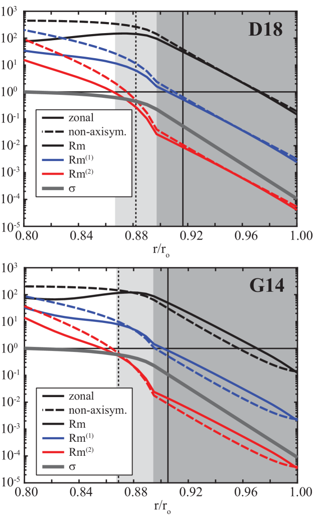
Figure 4: Radial profiles of the three different magnetic Reynolds numbers for snapshots of dynamo models D18 and G14. Solid (dashed) vertical lines mark the radii where Rm⁽¹⁾ (Rm⁽²⁾) exceed unity.

As already discussed in the introduction, the strong decrease in the electrical conductivity in the SDCR requires modified magnetic Reynolds numbers. In addition to profiled obeying the classical definition,

$$\mbox{Rm}(r)=\frac{\langle\mbox{$\mathbf{U}$}(r)\rangle\;d}{\lambda(r)}\;\;,$$ (21)

we will rely on

$$\mbox{Rm${}^{(1)}$}(r)=\frac{\langle\mbox{$\mathbf{U}$}(r)\rangle\;d_{\lambda}}{\lambda(r)}\;\;.$$ (22)

and also

$$\mbox{Rm${}^{(2)}$}(r)=\frac{\langle\mbox{$\mathbf{U}$}(r)\rangle\;d_{\lambda}^{2}}{\lambda(r)\;d}\;\;.$$ (23)

Here, $d_{\lambda}=\lambda/(\partial\lambda/\partial r)$ is the magnetic diffusivity scale height, and $\langle\mbox{U}(r)\rangle$ refers to the rms velocity on the sphere of radius $r$. In general, angular brackets indicate the spherical rms

$$\langle f(r)\rangle\>=\frac{1}{4\pi}\;\left(\int_{-1}^{1}dx\int_{0}^{2\pi}d\phi f^{2}\right)^{1/2}$$ (24)

throughout the paper, where $x=cos(\theta)$, $\theta$ is the colatitude and $\phi$ the longitude.

Fig. 4 compares the different magnetic Reynolds number profiles for the D18 and G14 snapshots, separating between zonal flow and non-axisymmetric flow contributions. Axisymmetric latitudinal and radial flows are typically much weaker and have thus been neglected here. While zonal and non-axisymmetric flows have comparable amplitudes in the SDCR of dynamo D18, zonal flows are somewhat more pronounced in model G14 because of the smaller Ekman number. In the exponential branch of the conductivity profiles, the diffusivity scale height assumes a constant value $d_{\lambda}=0.168$. This explains why the different Rm profiles in fig. 4 are parallel in the SDCR.

3 Dynamo Action in the SDCR

Ohm’s law,

$$\mbox{$\mathbf{j}$}=\sigma\left(\mbox{$\mathbf{U}$}\times\mbox{$\mathbf{B}$}+\mbox{$\mathbf{E}$}\right)\;\;,$$ (25)

states that the electric currents are driven by induction due to flow acting on magnetic field or by the electric field $\mathbf{E}$. Since both effects scale with $\sigma$, the current density $\mathbf{j}$ has to decays in the SDCR.

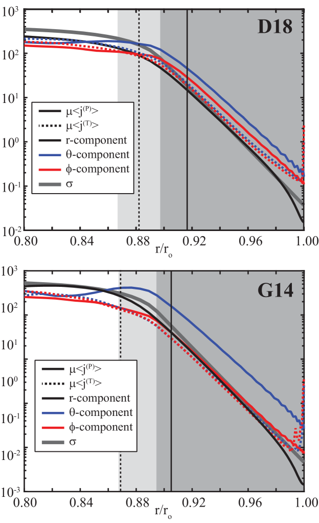
Figure 5: Radial profiles for the rms values of different current contributions. A scaled electrical conductivity profile is shown in gray. Background colors indicate the region where the conductivity is smaller than $50$% of its reference values at $r_{i}$ (light gray background) and the SDCR where is decays exponentially (mid gray background). Top and bottom panels show snapshots for dynamos D18 and G14, respectively. Solid (dashed) vertical lines mark the radii where Rm⁽¹⁾ (Rm⁽²⁾) exceed unity.

Fig. 5 illustrates the decay of the different current density components for the selected snapshots in dynamos D18 (top panel) and G14 (bottom panel). Shown are radial profiles of the rms values over spherical surfaces, indicated by angular brackets. The poloidal current (solid lines), more specifically its latitudinal component (solid blue), dominates in the SDCR. The poloidal current is at least two times larger than the toroidal current in model D18. The difference is even more pronounced in model G14, where the poloidal current is five times stronger than its toroidal counterpart, likely due to the stronger zonal flows. Radial currents (solid black) are effectively blocked off by the conductivity gradient and are thus generally small.

As expected, the decrease of the rms current density in the SDCR is mostly dictated by the electrical conductivity profile (thick gray line in fig. 5) with local induction effects providing some moderation. Below the SDCR, the current increases much more smoothly with depth and never exceeds twice the value reached at the bottom of the SDCR. The simple conductivity ruled gradients changes at a depth somewhere between $\mbox{Rm${}^{(1)}$}=1$ and $\mbox{Rm${}^{(2)}$}=1$ where more classical dynamo action kicks in.

In the simulations, we assume that the region $r>r_{o}$ is electrically insulating. The conditions that are gradually approached with increasing radius in the SDCR are finally abruptly enforced at $r_{o}$. Fig. 5 illustrates that this leads to a thin magnetic boundary layer where the simple dependence on $\sigma$ also brakes down. Another problem is that the very small currents in this very outer region cannot be calculated precisely enough, since we had to calculated from single precision magnetic field values stored in the snapshots.

In order to quantify the locally induced current-related poloidal field, we downward continue $\tilde{\mbox{$\mathbf{B}$}}$ below $r_{o}$ according to the characteristic radial dependence of a potential field:

$$\tilde{\mbox{$\mathbf{B}$}}_{\ell}(r)=\left(\frac{r_{o}}{r}\right)^{\ell+2}\;\mbox{$\mathbf{B}$}_{\ell}(r_{o})\;\;.$$ (26)

In the SDCR where local currents are small, the $\mathbf{B}$ remains close to $\tilde{\mbox{$\mathbf{B}$}}$. The difference

$$\hat{\mbox{$\mathbf{B}$}}^{(P)}(r)=\mbox{$\mathbf{B}$}^{(P)}(r)-\tilde{\mbox{$\mathbf{B}$}}(r)$$ (27)

provides a measure for the poloidal field produced by the local currents flowing beyond radius $r$. For simplicity, we will refer to $\hat{\mbox{$\mathbf{B}$}}$ as the non-potential poloidal field in the following.

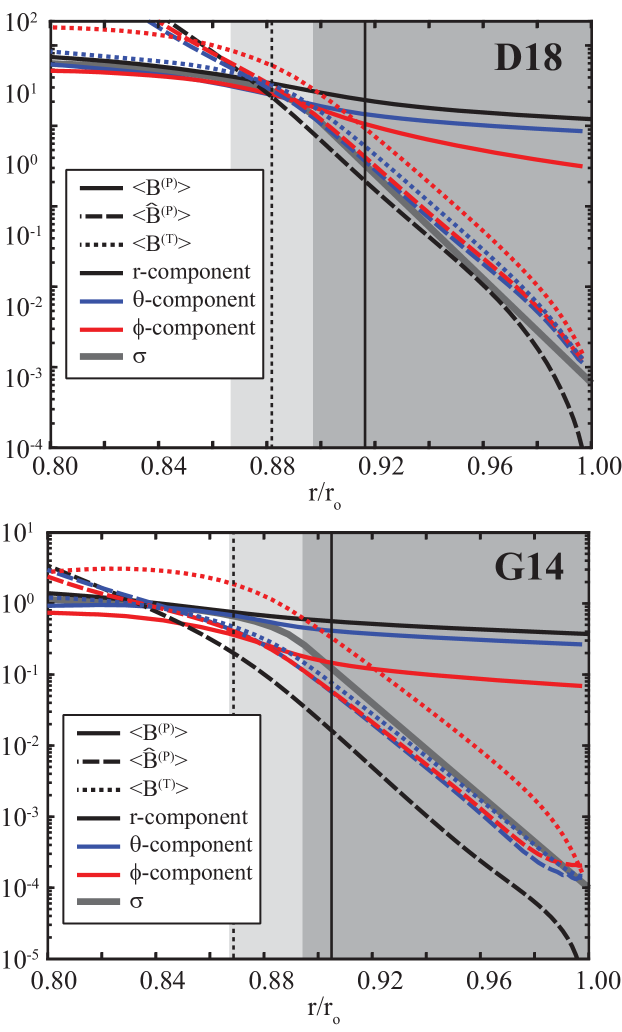
Figure 6: Rms values of different magnetic field contributions. See caption of fig. 5 for more explanation. Solid (dashed) vertical lines mark the radii where Rm⁽¹⁾ (Rm⁽²⁾) exceed unity. Dimensionless quantities shown.

Fig. 6 illustrates the radial dependence of different rms magnetic field contributions. The toroidal magnetic field connected to the poloidal currents dominates the non-potential field in the SDCR. The shear due to the zonal flow ($\omega$-effect) produces a particularly strong azimuthal toroidal field, an effect that is more pronounced in dynamo G14 than in D18. Since the rms azimuthal potential field is particularly weak, the locally induced field reaches a an amplitude comparable to $\langle\tilde{\mbox{B}}_{\phi}\rangle$ already within the SDCR. Using the downward continuation (26) to deduce $\hat{\mbox{$\mathbf{B}$}}$ stops to make sense when $\tilde{\mbox{$\mathbf{B}$}}$ becomes of the same order as $\mathbf{B}$. Fig. 6 shows that $\hat{\mbox{$\mathbf{B}$}}$ can even exceeds $\mathbf{B}$ below the SDCR. As we will further discuss below, the radius where Rm⁽¹⁾ exceeds unity, marked by a solid vertical line in fig. 6, is the depth where out approach brakes down.

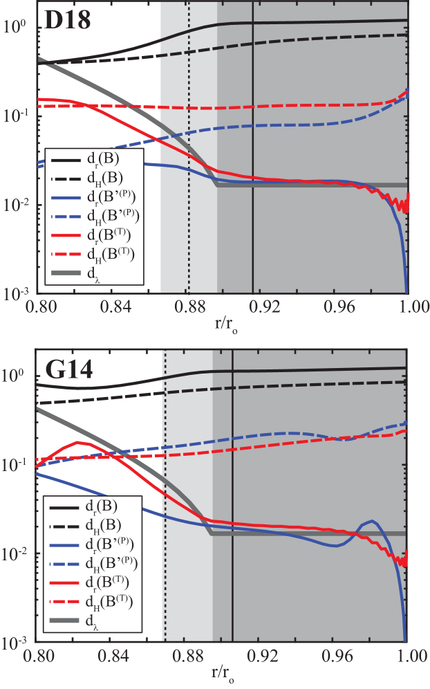
Figure 7: Radial (solid) and horizontal (dashed) rms scales of different field contributions. See caption of fig. 5 and the main text for more explanation.

Radial and horizontal magnetic field length scales, based on the respective derivatives of the field potentials, are illustrated in fig. 7. For example, the radial scale of the poloidal field is estimated via

$$d_{r}(B^{(p)})=\frac{\langle b^{(P)}\rangle}{\langle\partial b^{(P)}/\partial r\rangle}\;\;.$$ (28)

Horizontal scales have been calculated using the square root of $\langle\nabla_{H}^{2}g\rangle$. Between $r=0.90\,r_{o}$ and $r=0.97\,r_{o}$, the radial scale of $\hat{Bv}$ and the toroidal field is indeed very similar to the diffusive scale height $d_{\lambda}$, which confirms that the conductivity profile determines the non-potential magnetic field gradient. The horizontal length scales of both non-potential field contributions are significantly smaller than the respective scales of the total field (or the potential field) but still an order of magnitude larger than the radial scales.

The separate evolution equations for the toroidal and poloidal field potentials solved by MagIC are the radial component of the dynamo equation and the radial component of its curl (Christensen and Wicht, 2007),

$$\nabla_{H}^{2}\;\dot{b}^{(P)}=-\hat{\mathbf{r}}\cdot\left[\nabla\times\left(\mbox{$\mathbf{U}$}\times\mbox{$\mathbf{B}$}\right)\right]+\lambda\;\nabla_{H}^{2}\,\left[\left(\frac{\partial}{\partial r}\right)^{2}+\nabla_{H}^{2}\right]\;b^{(P)}$$ (29)

and

$$\nabla_{H}^{2}\;\dot{b}^{(T)}=-\hat{\mathbf{r}}\cdot\left[\nabla\times\nabla\times\left(\mbox{$\mathbf{U}$}\times\mbox{$\mathbf{B}$}\right)\right]+\lambda\;\nabla_{H}^{2}\,\left[\;\left(\frac{\partial}{\partial r}\right)^{2}+\nabla_{H}^{2}\;+\;\frac{1}{d_{\lambda}}\,\frac{\partial}{\partial r}\right]\;b^{(T)}\;\;.$$ (30)

Only the toroidal field equation directly includes the magnetic diffusivity scale height.

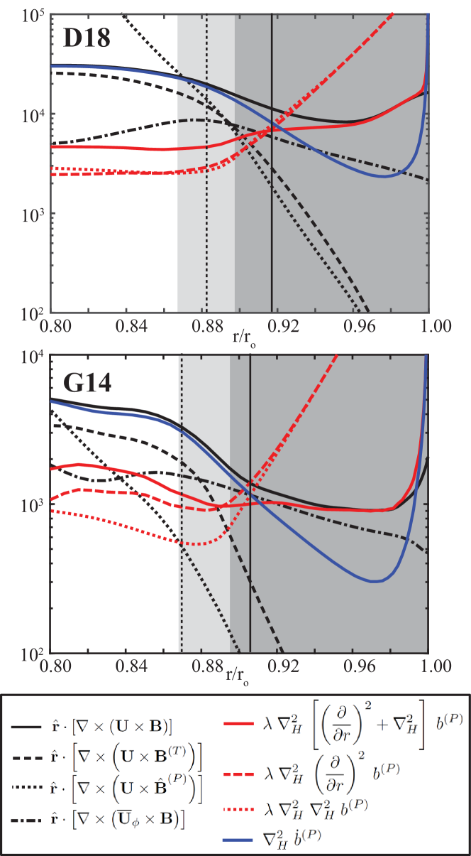
Figure 8: Horizontally averaged rms values of the different contributions to the poloidal dynamo equation for the snapshots in dynamos D18 (top) and G14 (bottom). The vertical lines mark where Rm⁽¹⁾ (solid) and Rm⁽²⁾ (dotted) reach unity. Dimensionless quantities shown.

Fig. 8 shows radial profiles of the rms values of the different contributions in the poloidal evolution equation for the D18 and G14 snapshots. Very close to the outer boundary beyond $r\approx 0.98\,r_{o}$, the use of single precision snap-shot data limits the quality of the second radial derivative required for the diffusive contributions. The balance should thus not be interpreted in this region.

We have separated the diffusive term into two contributions involving radial (red dashed line) and only horizontal (red dotted) derivatives. Both increase with $\lambda$ towards the outer boundary but also progressively cancel each other since the field approaches a potential field. What remains is the diffusive term for the non-potential field (red solid), which is mostly balanced by the induction term (black solid). Consequently, magnetic field variations (blue) become comparatively small in the highly diffusive SDCR.

Fig. 8 also illustrates that induction due to zonal flows (black dashed-dotted) is sizable for the poloidal field evolution. This describes pure advection of the background field $\tilde{\mbox{$\mathbf{B}$}}$. Induction due to flow acting on the toroidal field (black dashed) or the non-potential poloidal field (black dotted) on the other hand, remain minor contributions in the SDCR.

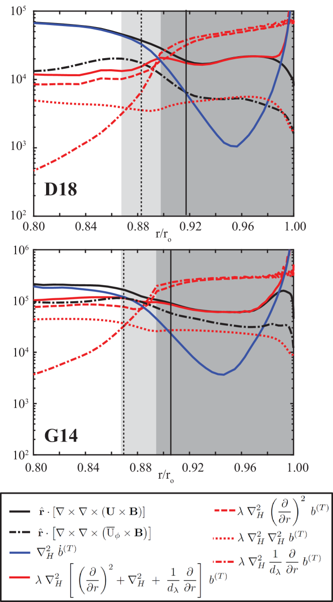
Figure 9: Horizontally averaged rms values of the different contributions to the toroidal dynamo equation for the snapshots in dynamos D18 (top) and G14 (bottom). The vertical lines mark where Rm⁽¹⁾ (solid) and Rm⁽²⁾ (dotted) reach unity. Dimensionless quantities shown.

For the rms balance in the toroidal field evolution, illustrated in fig. 9, time variations are even less important than for the poloidal counterpart. Note that the two dominant diffusive terms that involve radial derivatives (red dashed and dash-dotted lines) cancel to a high degree. This is simply a consequence of the fact that the toroidal field vanishes with $\sigma$ so that

$$\frac{\partial}{\partial r}\;b^{(T)}\approx-\frac{b^{(T)}}{d_{\lambda}}\;\;.$$ (31)

Zonal flows clearly dominate the toroidal field induction, in particular for dynamo G14.

Vertical lines in fig. 8 and fig. 9 again mark where the magnetic Reynolds numbers Rm⁽¹⁾ and Rm⁽²⁾ reach unity. The assumption of quasi stationary seems to be limited to the region $\mbox{Rm${}^{(1)}$}>1$. Where Rm⁽²⁾ reaches unity at a somewhat greater depth, the induction term already clearly dominates diffusion and the dynamics is decisively non-stationary.

4 Estimating the Dynamo Action

The analysis of dynamo simulations has shown that the dynamo action in the SDCR  is dominated by diffusive effects and thus obeys a quasi-stationary dynamics. In this section, we exploit this simplicity and derive estimates which could be used to estimate the dynamo action in the SDCR of planets.

4.1 Estimating the Electric Currents

The decent balance between diffusion and induction in the dynamo equation suggests

$$\left(\nabla\times\sigma\mbox{$\mathbf{j}$}\right)\approx-\nabla\times\left(\mbox{$\mathbf{U}$}\times\tilde{\mbox{$\mathbf{B}$}}\right)\;\;.$$ (32)

When using the fact that radial derivatives dominate in the SDCR, this leads to the radial integral estimate $\mbox{$\boldsymbol{\mathcal{J}}$}_{H}$ for the horizontal currents used by (Liu et al., 2008):

$$\mbox{$\mathbf{j}$}_{H}(r)\approx\mbox{$\boldsymbol{\mathcal{J}}$}_{H}(r)=\sigma\;\int_{r}^{r_{o}}\,dr^{\prime}\;\hat{\mathbf{r}}\times\left[\nabla\times\left(\mbox{$\mathbf{U}$}\times\tilde{\mbox{$\mathbf{B}$}}\right)\right]_{H}\;+\;C_{H}\;\;.$$ (33)

Here $C_{h}$ stands for the integration constants which guarantees that the current vanishes for $r=r_{o}$.

A simpler estimate can be based on Ohm’s law. Balance (32) already suggest that electric field contributions associated to variation in the magnetic field via the Maxwell-Faraday law, $\partial\mbox{$\mathbf{B}$}/\partial t=-\nabla\times\mbox{$\mathbf{E}$}$, are small. A second possible contribution are potential field gradient, $\mbox{E}=-\nabla V$. At least the latitudinal component of $\mbox{$\mathbf{U}$}\times\mbox{$\mathbf{B}$}$ clearly dominates the respective electric field contribution and the fast zonal flows likely also play a role here. This suggest to use the simplified Ohm’s law for a fast moving conductor:

$$\mbox{$\mathbf{j}$}\approx\sigma\;\mbox{$\mathbf{U}$}\times\tilde{\mbox{$\mathbf{B}$}}\;\;.$$ (34)

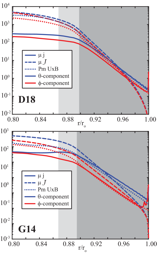
Figure 10: Radial profiles of the rms horizontal current densities along with two different estimates. Dimensionless quantities shown.

Fig. 10 illustrates that the rms horizontal currents in the SDCR are indeed close to the rms value of $\sigma\mbox{$\mathbf{U}$}\times\mbox{$\mathbf{B}$}$ (dotted lines) with deviations below $50$% for $r>0.90\,r_{o}$. The integral estimate $\mbox{$\boldsymbol{\mathcal{J}}$}_{H}$, shown as dashed lines in fig. 10, provides a somewhat inferior estimate but nevertheless correctly captures the order of magnitude. Below the SDCR, however, $\sigma\mbox{$\mathbf{U}$}\times\mbox{$\mathbf{B}$}$ is much larger than $\mathbf{j}$ and the electric field (or magnetic field variations) can definitely not be neglected.

While eqn. (34) convincingly approximates the horizontal currents densities, it severely overestimates the much weaker radial component. We can, however, use the fact that the currents are predominantly poloidal. Taking the horizontal divergence of eqn. (34) yields

$$\nabla_{H}^{2}\frac{\partial}{\partial r}j^{(p)}\approx\sigma\;\nabla_{H}\cdot\left(\mbox{$\mathbf{U}$}\times\mbox{$\mathbf{B}$}\right)_{H}\;\;.$$ (35)

This suggest the alternative integral estimate

$$J_{r}(r)\approx\mbox{$\mathcal{J}$}_{r}(r)=-\int_{r}^{r_{o}}dr^{\prime}\;\sigma\;\nabla_{H}\cdot\left(\mbox{$\mathbf{U}$}\times\mbox{$\mathbf{B}$}\right)_{H}+C_{r}\;\;,$$ (36)

where $C_{r}$ is an integration constant used to assure that $J_{r}$ vanishes at $r_{o}$. Since the gradient in $\sigma$ will dominate the integral, the simplified expression

$$J_{r}\approx d_{\lambda}\sigma\;\nabla_{H}\cdot\left(\mbox{$\mathbf{U}$}\times\tilde{\mbox{$\mathbf{B}$}}\right)_{H}$$ (37)

provides a very decent estimate.

For estimating the rms electrical current, we rely on the estimate for the dominant horizontal component. Using background field $\tilde{\mbox{$\mathbf{B}$}}$ and ignoring the cross product in eqn. (34) leads to

$$\langle\mbox{$\mathbf{J}$}\rangle\approx\sigma\;\langle\mbox{$\mathbf{U}$}\rangle\;\langle\tilde{\mbox{$\mathbf{B}$}}\rangle=\frac{\mbox{Rm}}{\mu\,d}\;\langle\tilde{\mbox{$\mathbf{B}$}}\rangle\;\;,$$ (38)

while only slightly degrading the estimate. To quantify its quality, we calculate the ratio of the estimate to the true value,

$$R_{J}=\frac{\sigma\,\langle\mbox{$\mathbf{U}$}\rangle\,\langle\tilde{\mbox{$\mathbf{B}$}}\rangle}{\langle\mbox{$\mathbf{J}$}\rangle}\;\;.$$ (39)

For the radial component, the ratio based on eqn. (37) reads

$$R_{Jr}=d_{\lambda}\,\sigma\frac{\langle\nabla_{H}\cdot\left(\mbox{$\mathbf{U}$}\times\tilde{\mbox{$\mathbf{B}$}}\right)_{H}\rangle}{\langle\mbox{J}_{r}\rangle}\;\;.$$ (40)

Ignoring cross product and divergence in eqn. (37) yields the simpler estimate

$$\langle J_{r}\rangle\approx\sigma\;\frac{d_{\lambda}}{d}\langle\mbox{$\mathbf{U}$}\rangle\langle\tilde{\mbox{$\mathbf{B}$}}\rangle=\frac{\mbox{Rm${}^{(1)}$}}{\mu\,d}\;\langle\tilde{\mbox{$\mathbf{B}$}}\rangle$$ (41)

with the respective ratio

$$\hat{R}_{Jr}=\frac{\sigma d_{\lambda}\,\langle\mbox{$\mathbf{U}$}\rangle\,\langle\tilde{\mbox{$\mathbf{B}$}}\rangle}{d\,\langle\mbox{$\mathbf{J}$}\rangle}\;\;.$$ (42)

Fig. 11 shows the mean values and standard deviations for the different ratios when using 14 snapshots for D18 and $10$ for G14. When using Ohm’s law for a fast moving conductor, the rms currents are overestimated by factors between $1.5$ and $2.5$ for $r>0.92r_{o}$ (solid lines in fig. 11a). The quality of the integral estimate, however, varies significantly with depth and provides reasonable values for $0.91\,r_{o}<r<0.96\,r_{o}$. Estimates for the smaller radial current are of generally high quality when including the divergence in (37) (solid lines in fig. 11b). Ignoring the divergence, however, leads to values that are about an order of magnitude too low (dotted lines in fig. 11b).

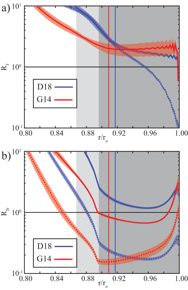
Figure 11: Ratio of estimates and true rms electric current density. The results have been averaged over 14 snapshots for dynamo D18 and 10 snapshots for dynamo G14. Transparent background stripes with a width of two standard deviations illustrate the variability. The vertical lines mark where Rm⁽¹⁾ (solid) or Rm⁽²⁾ (dotted) exceed one. Panel a) shows ratio (39) for the simplified estimate based on Ohm’s law (solid lines) and an respective ratio for the integral estimate (33) $\mbox{$\boldsymbol{\mathcal{J}}$}_{H}$ (dotted lines). Panel b) compares ratios (37) (full lines) and (41) (dotted lines) for the radial current contributions.

Fig. 11 also suggest that the estimates remain more or less valid throughout the whole SDCR. The assumption of a dominant dominant background potential field but also for the quasi-stationary dynamo action roughly holds for $\mbox{Rm${}^{(1)}$}\geq 1$ and the radii where Rm⁽¹⁾ reaches unity have been marked with vertical lines in fig. 11. The validity of our estimates extends to slightly greater depth, reaching $\mbox{Rm${}^{(1)}$}\approx 2$ and $\mbox{Rm${}^{(1)}$}\approx 1.5$ at the bottom of the SDCR for dynamos D18 and G14, respectively. Where $\mbox{Rm${}^{(2)}$}\approx 1$, however, the estimates are definitely off.

Figure 12: Pearson correlation coefficients between individual current density components and two different estimates. Solid lines refer to the estimates based on the simplified Ohm’s law (34) while dotted lines refer to the integral expression (33) for the horizontal and (37) for the radial component.

To access whether the estimates not only capture the rms amplitudes but also the structure, we calculate the Pearson correlation coefficients for each radius, for example

$$C(\mbox{J}_{\theta},\sigma(\mbox{$\mathbf{U}$}\times\mbox{$\mathbf{B}$})_{\theta})=\frac{\overline{\left(\mbox{J}_{\theta}-\overline{\mbox{J}}_{\theta}\right)\;\left(\left[\mbox{$\mathbf{U}$}\times\mbox{$\mathbf{B}$}\right]_{\theta}-\overline{\left[\mbox{$\mathbf{U}$}\times\mbox{$\mathbf{B}$}\right]}_{\theta}\right)}}{\left[\overline{\left(\mbox{J}_{\theta}-\overline{\mbox{J}}_{\theta}\right)^{2}}\;\;\overline{\left(\left[\mbox{$\mathbf{U}$}\times\mbox{$\mathbf{B}$}\right]_{\theta}-\overline{\left[\mbox{$\mathbf{U}$}\times\mbox{$\mathbf{B}$}\right]}_{\theta}\right)^{2}}\right]^{1/2}}\;\;,$$ (43)

where the overbars refer to an average over a spherical surface. The results, shown in fig. 12, demonstrate that $\sigma\mbox{$\mathbf{U}$}\times\mbox{$\mathbf{B}$}$ no only provides a better rms estimate but also a better local estimate than $\mbox{$\boldsymbol{\mathcal{J}}$}_{H}$ for the horizontal current components. Particularly high correlations are reached for the latitudinal current density in G14 where the zonal flow contributes most strongly. For the radial component, eqn. (36) also provides a decent local estimate with Pearson coefficients up to $0.85$ for G14.

Fig. 13 illustrates the close agreement for the latitudinal current density in model G14 at $r=0.94\,r_{o}$. The banded structure due to the zonal flow action already reported by Gastine et al. (2014b) is clearly apparent.

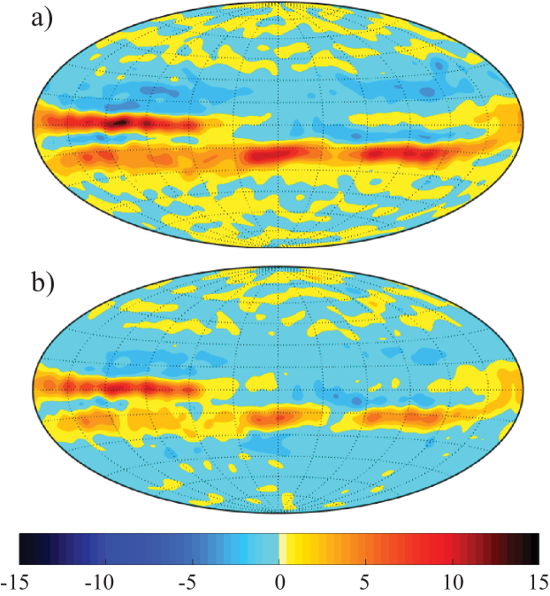
Figure 13: Comparison of a) $\mu J_{\theta}$ with b) estimate $\mbox{Pm}(\mbox{$\mathbf{U}$}\times\mbox{$\mathbf{B}$})_{\theta}$ at $r=0.94\,r_{o}$ for the snapshot of dynamo G14. Dimensionless quantities shown.

4.2 Estimating the Non-Potential Field

The toroidal and the non-potential poloidal fields can be assessed by uncurling Ampere’s law $\nabla\times\mbox{$\mathbf{B}$}=\mu\mbox{$\mathbf{j}$}$. This becomes particularly simple in the SDCR where the radial field gradients clearly dominate so that

$$\hat{\mathbf{r}}\times\frac{\partial}{\partial r}\mbox{$\mathbf{B}$}_{H}\approx\mu\mbox{$\mathbf{j}$}_{H}\;\;.$$ (44)

Integrating this expression from $r_{o}$ to $r$ yields the integral approximation $\mbox{$\boldsymbol{\mathcal{B}}$}_{J}$,

$$\hat{\mbox{$\mathbf{B}$}}_{H}(r)\approx\mbox{$\boldsymbol{\mathcal{B}}$}_{H}(r)\>=\mu\;\int_{r}^{r_{o}}\,dr^{\prime}\;\hat{\mathbf{r}}\times\mbox{$\mathbf{j}$}_{H}\;\;,$$ (45)

where the integration constant has been set to zero, assuming that $\hat{\mbox{$\mathbf{B}$}}_{H}$ and the current vanish at $r_{o}$.

Separating the current into poloidal and toroidal contributions allows for individually estimating the toroidal and poloidal non-potential fields. Both aggree very well with the horizontal components of the toroidal field and the non-potential poloidal field $\hat{\mbox{$\mathbf{B}$}}^{(P)}$ in the SDCR, as is demonstrated in fig. 14. The radial integral (45) continues to provide a good representation of the toroidal field even below the SDCR.

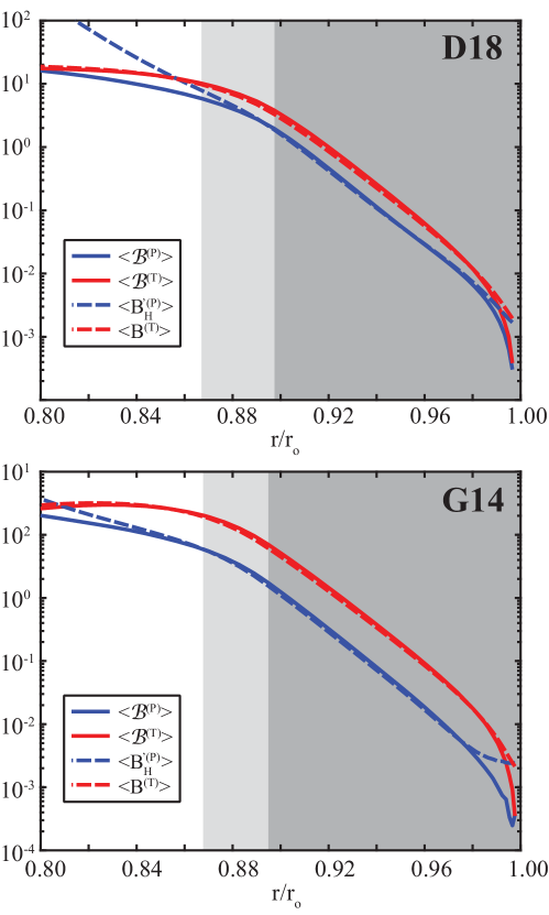
Figure 14: Comparison of the rms values for the integral estimates from uncurling Ampere’s law with the rms toroidal field $\langle\mbox{$\mathbf{B}$}^{(T)}\rangle$ and the rms horizontal non-potential field $\langle\hat{\mbox{$\mathbf{B}$}}_{H}\rangle$. Dimensionless quantities shown.

Combining these integral expressions with the current approximation via the simplified Ohm’s law yields the integral estimate $\mbox{$\boldsymbol{\mathcal{B}}$}_{O}$:

$$\hat{\mbox{$\mathbf{B}$}}_{H}(r)\approx\mbox{$\boldsymbol{\mathcal{B}}$}_{O}(r)\>=\;\int_{r}^{r_{o}}\,dr\;\;\frac{\hat{\mathbf{r}}\times\left(\mbox{$\mathbf{U}$}\times\mbox{$\mathbf{B}$}\right)}{\lambda}\;\;.$$ (46)

The dominance of the radial dependence of $\lambda$ then suggests

$$\hat{\mbox{$\mathbf{B}$}}_{H}(r)\approx\mbox{$\boldsymbol{\mathcal{B}}$}_{O}(r)\>=\frac{d_{\lambda}}{\lambda}\;\hat{\mathbf{r}}\times\left(\mbox{$\mathbf{U}$}\times\mbox{$\mathbf{B}$}\right)\;\;.$$ (47)

and an rms value of

$$\langle\hat{\mbox{$\mathbf{B}$}}\rangle\approx\mbox{Rm${}^{(1)}$}\langle\tilde{\mbox{$\mathbf{B}$}}\rangle\;\;.$$ (48)

For estimating the poloidal field we rely on the respective dynamo equation eqn. (29). Since radial derivatives clearly dominate, the stationary radial component of the dynamo equation reduces to

$$\lambda\;\left(\frac{\partial}{\partial r}\right)^{2}\;\hat{\mbox{B}}_{r}\approx-\hat{\mathbf{r}}\cdot\nabla\times\left(\mbox{$\mathbf{U}$}\times\tilde{\mbox{$\mathbf{B}$}}\right)\;\;,$$ (49)

where we have used the potential background field on the right hand side. The diffusive left hand side can reasonably be approximated with $\lambda\hat{\mbox{B}}_{r}/d_{\lambda}^{2}$, which yields

$$\hat{\mbox{B}}_{r}\approx-\frac{d_{\lambda}^{2}}{\lambda}\;\hat{\mathbf{r}}\cdot\nabla\times\left(\mbox{$\mathbf{U}$}\times\tilde{\mbox{$\mathbf{B}$}}\right)\;\;.$$ (50)

The quality of estimates eqn. (48) and eqn. (50) will be quantified by the ratios

$$R_{B}=\mbox{Rm${}^{(1)}$}\frac{\langle\tilde{\mbox{B}}\rangle}{\langle\hat{\mbox{$\mathbf{B}$}}\rangle}$$ (51)

and

$$R_{Br}=\frac{d_{\lambda}^{2}}{\lambda}\frac{\langle\hat{\mathbf{r}}\cdot\nabla\times\left(\mbox{$\mathbf{U}$}\times\tilde{\mbox{$\mathbf{B}$}}\right)\rangle}{\langle\hat{\mbox{B}}_{r}\rangle}\;\;,$$ (52)

respectively. A simplified expression ignoring the curl and cross product yields

$$\langle\hat{\mbox{B}}_{r}\rangle\approx\mbox{Rm${}^{(2)}$}\langle\tilde{\mbox{$\mathbf{B}$}}\rangle\;\;,$$ (53)

with the respective ratio

$$\hat{R}_{Br}=\mbox{Rm${}^{(2)}$}\frac{\langle\tilde{\mbox{$\mathbf{B}$}}\rangle}{\langle\hat{\mbox{B}}_{r}\rangle}\;\;.$$ (54)

Fig. 15 shows that very reasonable values between $R_{B}=1.3$ and $R_{B}=2$ for the total non-potential field and between $R_{Br}=0.8$ and $R_{B_{r}}=2$ for its radial contributions are achieved in the SDCR, ignoring once more the very outer few percent in radius. In terms of magnetic Reynolds numbers, the region where the estimates offer acceptable results extends to a depth between $\mbox{Rm${}^{(1)}$}=1$ and $\mbox{Rm${}^{(2)}$}=1$ (see vertical lines in fig. 15.

The simplified estimate (54), on the other hand, underestimates the radial non-potential field by a factor three for dynamo D18, which has a particularly small scale background field $\tilde{\mbox{$\mathbf{B}$}}$. For dynamo G14, the simplification has a much smaller effect and the quality of the estimate is only mildly affected.

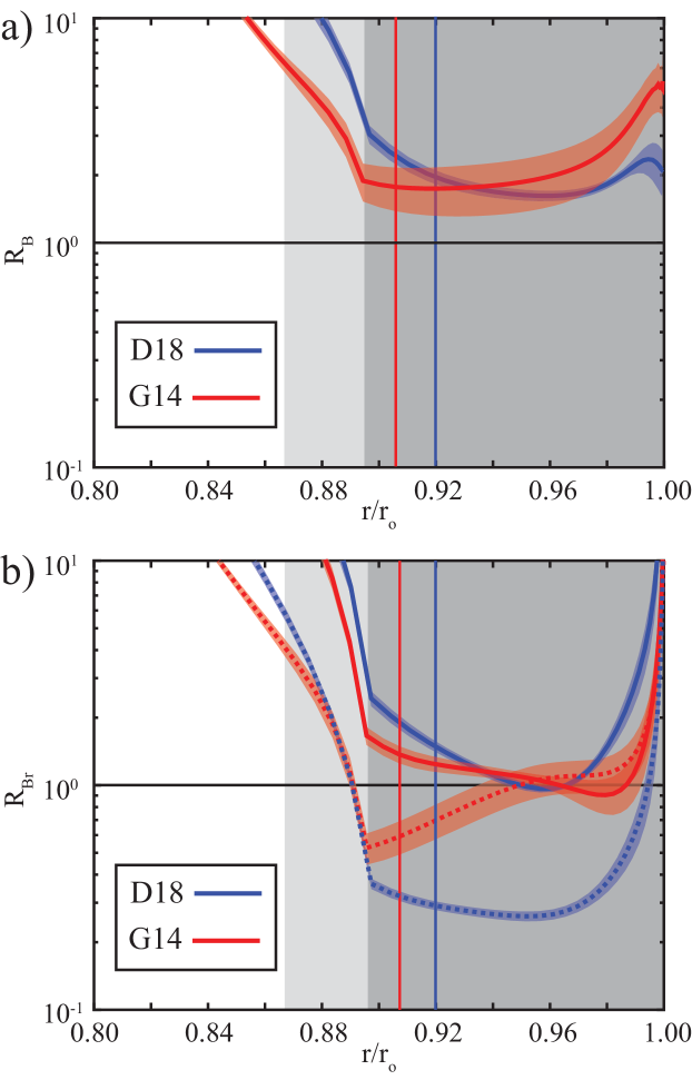
Figure 15: Ratio of rms values for the non-potential radial field estimate 50 and for $\hat{\mbox{B}}_{r}$. Results have been averaged over 14 snapshots for dynamo D18 and 9 snapshots for dynamo G14. Transparent background stripes with a width of two standard deviations illustrate the variability. The vertical lines mark where Rm⁽¹⁾ (solid) or Rm⁽²⁾ (dotted) exceed one.

The Pearson correlation coefficients in the SDCR range between $0.5$ and $0.9$ for the non-potential radial field estimate, and between $0.6$ and $0.8$ for the non-potential azimuthal field estimate, as is illustrated in fig. 16. For the weak latitudinal field, however, the estimate is much less reliable. Fig. 17 illustrates the good agreement between $\hat{\mbox{B}}_{r}$ and estimate (50) for the G14 snapshot. The banded structure becomes once more apparent, but the field is much more small scale owed to the complex convective flows that provide the main radial field induction (Gastine et al., 2014b).

Figure 16: Peason correlation coefficients between individual magnetic field components and respective estimates.

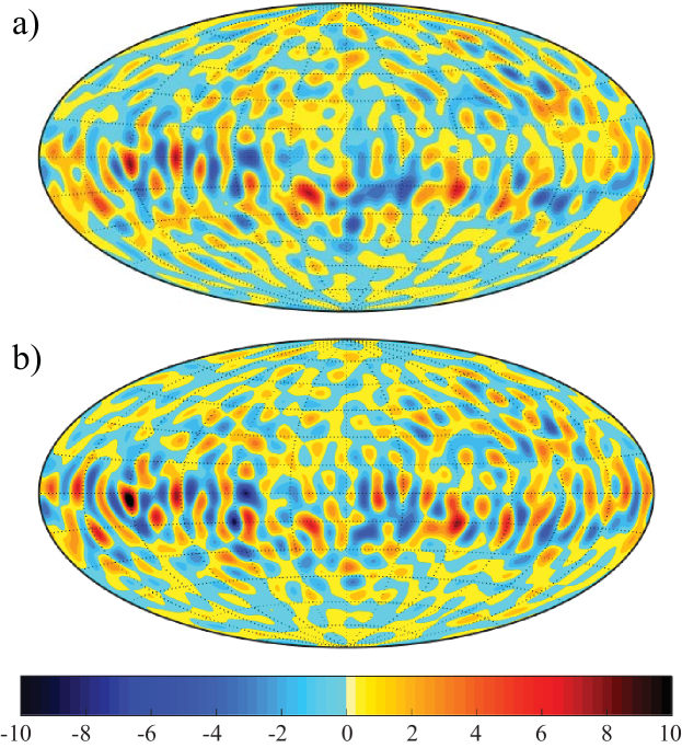
Figure 17: Comparison of a) $\hat{\mbox{B}}_{r}$ with b) estimate eqn. (50) for $r=0.94r_{o}$ and a snapshot for dynamo G14. Dimensionless quantities shown.

4.3 Estimating the Lorentz Force

Having derived estimates for electric currents and magnetic fields, we can combine both to also assess the Lorentz force $\mathbf{L}$ in the SDCR. Of particular interest is its zonal (axisymmetric azimuthal) component $\overline{L}_{\phi}$ which could potentially impact the zonal winds. Fig. 18 shows the profiles of the rms contributions to $\langle\overline{L}_{\phi}\rangle$ for dynamos D18 and G14. The figure illustrates that from the two contributions,

$$\overline{L}_{\phi}=\overline{J_{r}B_{\theta}}-\overline{J_{\theta}B_{r}}\;\;,$$ (55)

the second clearly dominates because of the higher latitudinal current density.

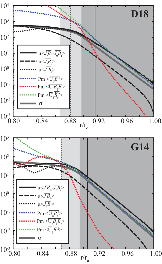
Figure 18: Zonal rms Lorentz force contributions and estimates. See text for more explanation. Dimensionless quantities shown.

Combining the estimates for $J_{\theta}$ and $B_{r}$ then suggest

$$\overline{L}_{\phi}\approx-\sigma\;\overline{\left(\mbox{$\mathbf{U}$}\times\mbox{$\mathbf{B}$}\right)_{\theta}\mbox{B}_{r}}=-\sigma\;\overline{\mbox{U}_{\phi}\mbox{B}_{r}^{2}}+\sigma\;\overline{\mbox{U}_{r}\mbox{B}_{\phi}\mbox{B}_{r}}\;\;.$$ (56)

Fig. 18 illustrates that the first contribution dominates, in particular for model G14 where zonal flows are stronger. We can thus estimate the rms zonal Lorentz force based on a conductivity model, a zonal flow model, and the potential field:

$$\langle\overline{L}_{\phi}\rangle\approx\sigma\;\langle\overline{\mbox{U}}_{\phi}\rangle\;\langle\overline{\tilde{\mbox{B}}^{2}_{r}}\rangle\;\;,$$ (57)

The respective ratio

$$R_{LF}=\frac{\sigma\;\langle\overline{\mbox{U}}_{\phi}\rangle\;\langle\overline{\tilde{\mbox{B}}_{r}^{2}}\rangle}{\langle\overline{L}_{\phi}\rangle}\;\;,$$ (58)

shown in fig. 19, demonstrates that this expression tends to underestimate the zonal Lorentz force by only up to $40$%. The region where this estimates can reasonable be applied is larger for G14 where zonal flows are stronger.

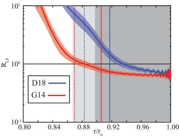
Figure 19: Ratio of estimate (57) to the zonal Lorentz force. Thick lines show averages over 14 snapshots for dynamo D18 (blue) and 10 snapshots for dynamo G14 (red). The transparent background stripes with a width of twice the standard deviation illustrate the variability. Thin vertical lines show where Rm⁽¹⁾ (solid) or Rm⁽²⁾ (dotted) exceed one.

5 Discussion and Conclusion

The analysis of our numerical simulations shows that dynamo action in the Steeply Decaying Conductivity Region (SDCR) is dominated by Ohmic dissipation. The magnetic field dynamics becomes quasi stationary with a good balance between induction and diffusion. Ohm’s law, on the other hand, assumes the simplified form for a fast moving conductor, where the electric field can be neglected. Electric currents and the toroidal field simply decay with the electrical conductivity, while the poloidal field approaches a potential field.

This particular situation allows to formulate rather simple estimates based on the knowledge of the surface field, the conductivity profile, and the flow. The electric current density can be estimated via the simplified Ohm’s law with a suggested rms value of $\langle\mbox{$\mathbf{J}$}\rangle\approx\sigma\langle\mbox{$\mathbf{U}$}\rangle\;\langle\tilde{\mbox{$\mathbf{B}$}}\rangle$, where $\tilde{\mbox{$\mathbf{B}$}}$ is the downward continued surface field under the potential field assumption. The accuracy is higher than the more classical estimate used by Liu et al. (2008) for their assessment of Ohmic heating due to Jupiter’s zonal winds.

Also of interest is the locally induced radial magnetic field that could potentially be detected by the Juno spacecraft. Our analysis shows that $\langle\mbox{B}^{\prime}_{r}\rangle\approx\mbox{Rm${}^{(2)}$}\langle\tilde{\mbox{$\mathbf{B}$}}\rangle$ provides a reasonable estimate, where Rm⁽²⁾ is a modified magnetic Reynolds number that depends on the square of the diffusivity scale height $d_{\lambda}$. The locally induced toroidal field, on the other hand, can be predicted via $\langle\mbox{$\mathbf{B}$}\rangle\approx\mbox{Rm${}^{(1)}$}\langle\tilde{\mbox{$\mathbf{B}$}}\rangle$ and is thus by a factor $\mbox{Rm${}^{(1)}$}/\mbox{Rm${}^{(2)}$}=d/d_{\lambda}$ larger than the radial field. When using the conductivity model by French et al. (2012), this predicts that the locally induced toroidal field is about $10^{3}$ time larger than the locally induced radial field at $0.96\,r_{J}$. At $0.9\,r_{J}$, this ratio has decreased to $10^{2}$.

While the toroidal field estimate agrees with the assessment by Cao and Stevenson (2017), the poloidal field estimates differ. Cao and Stevenson (2017) consider the poloidal field produced by non-axisymmetric (helical) flows acting on the local toroidal field, but the advective modification of $\tilde{\mbox{$\mathbf{B}$}}$ turns out to be significantly larger in the SDCR of our simulations.

Duarte et al. (2018) define the top of the dynamo region $r_{D}$ based on a critical magnetic Reynolds number. A more reasonable local definition is the depth where the local magnetic effects reach a certain threshold. Since the electric current, toroidal field, and radial field all scale with different magnetic Reynolds numbers, the answer will actually depend on the quantity considered.

Choosing the radial magnetic field has the advantages that it is most directly connected to magnetic field observations. For the most recent field models based on Juno data, Connerney et al. (2018) discuss an $r_{D}$ value of $0.85\,r_{J}$. The authors argue that the spectrum of $\tilde{\mbox{$\mathbf{B}$}}$ is close to a white spectrum at this depth, a criterion that successfully predicts Earth’s core-mantle boundary when excluding the axial dipole contribution. However, $0.85\,r_{J}$ lies below the transition to the metallic Hydrogen region (French et al., 2012) and below the anticipated depth of the zonal winds (Kaspi et al., 2018). Assuming a mean convective velocity of $3\,$cm/s (Gastine et al., 2014b) and the French conductivity profile predicts $\mbox{Rm${}^{(1)}$}=2.7\times 10^{4}$ and $\mbox{Rm}=7.6\times 10^{5}$ at $0.85\,r_{J}$. These huge values suggest that dynamo action should already be more than well developed.

The respective Rm⁽¹⁾ profile actually exceeds unity at about $0.93\,r_{J}$, which will therefore roughly mark the depth the estimates discussed here start to loose their basis. Since Rm⁽²⁾ is about $10^{-4}$ at $0.93\,r_{J}$ and the potential field amplitude is about $1\,$mT, the locally induced radial field would be roughly $10^{-4}\,$mT.

However, these considerations ignore the zonal winds, which reach amplitudes of around $150\,$m/s at Jupiter’s cloud level. Recent consideration based on Juno’s gravity measurements constrain the depth profile of the zonal winds and suggest a considerably lower wind speed at about $0.96\,r_{J}$. In a forthcoming paper, we use the estimates derived here in combination with the new depth profiles for the zonal winds to predict the zonal flow induced magnetic fields and electric currents and also calculate the related Ohmic heating. The analysis presented here suggest that decent local estimates are also possible. The predicted maps of Ohmic heating and radial field modifications could be compared with spacecraft observation to detect potential zonal field induction effects.

The questions addressed here are also of interest for other planets where fast fluid flows correlate with a region of decaying electrical conductivity. Saturn, Uranus, and Neptune, come to mind. The Ohmic heating in the outer atmospheres of hot-Jupiters, where the ionization of alkali metals creates a SDCR, is a possible mechanism to explain the particularly low density (inflation) of some of these exoplanets. Batygin and Stevenson (2010) assume a stationary dynamo equation to estimate that the locally induced currents would indeed provide sufficient heating power. Our result suggest that their approach and thus also likely their conclusions are viable.

References

- Batygin and Stevenson (2010) Batygin, K., Stevenson, D. J., May 2010. Inflating Hot Jupiters with Ohmic Dissipation. Astrophys. J. 714, L238–L243.
- Braginsky and Roberts (1995) Braginsky, S., Roberts, P., 1995. Equations governing convection in Earth’s core and the geodynamo. Geophys. Astrophys. Fluid Dyn. 79, 1–97.
- Cao and Stevenson (2017) Cao, H., Stevenson, D. J., Apr. 2017. Gravity and zonal flows of giant planets: From the Euler equation to the thermal wind equation. J. Geophys. Res. 122, 686–700.
- Christensen and Aubert (2006) Christensen, U., Aubert, J., 2006. Scaling properties of convection-driven dynamos in rotating spherical shells and applications to planetary magnetic fields. Geophys. J. Int. 116, 97–114.
- Christensen and Wicht (2007) Christensen, U., Wicht, J., 2007. Numerical dynamo simulations. In: P., O. (Ed.), Core Dynamics, second edt. Edition. Vol. 8 of Treatise on Geophysics. Elsevier, pp. 245–282.
- Connerney et al. (2018) Connerney, J. E. P., Kotsiaros, S., Oliversen, R. J., Espley, J. R., Joergensen, J. L., Joergensen, P. S., Merayo, J. M. G., Herceg, M., Bloxham, J., Moore, K. M., Bolton, S. J., Levin, S. M., Mar. 2018. A New Model of Jupiter’s Magnetic Field From Juno’s First Nine Orbits. Geophys. Res. Lett. 45, 2590–2596.
- Duarte et al. (2013) Duarte, L. D. V., Gastine, T., Wicht, J., Sep. 2013. Anelastic dynamo models with variable electrical conductivity: An application to gas giants. Phys. Earth Planet. Inter. 222, 22–34.
- Duarte et al. (2018) Duarte, L. D. V., Wicht, J., Gastine, T., Jan. 2018. Physical conditions for Jupiter-like dynamo models. Icarus 299, 206–221.
- French et al. (2012) French, M., Becker, A., Lorenzen, W., Nettelmann, N., Bethkenhagen, M., Wicht, J., Redmer, R., Sep. 2012. Ab Initio Simulations for Material Properties along the Jupiter Adiabat. Astrophys. J. Supp. 202, 5.
- Gastine et al. (2012) Gastine, T., Duarte, L., Wicht, J., october 2012. Dipolar versus multipolar dynamos: the influence of the background density stratification. Astron. Atrophys. 546, A19.
- Gastine et al. (2014a) Gastine, T., Heimpel, M., Wicht, J., Jul. 2014a. Zonal flow scaling in rapidly-rotating compressible convection. Phys. Earth Planet. Inter. 232, 36–50.
- Gastine and Wicht (2012) Gastine, T., Wicht, J., may 2012. Effects of compressibility on driving zonal flow in gas giants. Icarus 219, 428–442.
- Gastine et al. (2014b) Gastine, T., Wicht, J., Duarte, L. D. V., Heimpel, M., Becker, A., Aug. 2014b. Explaining Jupiter’s magnetic field and equatorial jet dynamics. Geophys. Res. Lett. 41, 5410–5419.
- Jones et al. (2011) Jones, C. A., Boronski, P., Brun, A. S., Glatzmaier, G. A., Gastine, T., Miesch, M. S., Wicht, J., Nov. 2011. Anelastic convection-driven dynamo benchmarks. Icarus 216, 120–135.
- Kaspi et al. (2018) Kaspi, Y., Galanti, E., Hubbard, W. B., Stevenson, D. J., Bolton, S. J., Iess, L., Guillot, T., Bloxham, J., Connerney, J. E. P., Cao, H., Durante, D., Folkner, W. M., Helled, R., Ingersoll, A. P., Levin, S. M., Lunine, J. I., Miguel, Y., Militzer, B., Parisi, M., Wahl, S. M., Mar. 2018. Jupiter’s atmospheric jet streams extend thousands of kilometres deep. Nature 555, 223–226.
- Liu et al. (2008) Liu, J., Goldreich, P. M., Stevenson, D. J., Aug. 2008. Constraints on deep-seated zonal winds inside Jupiter and Saturn. Icarus 196, 653–664.
- Nettelmann et al. (2012) Nettelmann, N., Helled, R., Fortney, J. J., Redmer, R., Jul. 2012. New indication for a dichotomy in the interior structure of Uranus and Neptune from the application of modified shape and rotation data. ArXiv e-prints.
- Ridley and Holme (2016) Ridley, V. A., Holme, R., Mar. 2016. Modeling the Jovian magnetic field and its secular variation using all available magnetic field observations. J. Geophys. Res. 121, 309–337.
- Wicht et al. (2018) Wicht, J., French, M., Stellmach, S., Nettelmann, N., Gastine, T., Duarte, L., Redmer, R., 2018. Modeling the interior dynamics of gas planets. In: Lühr, H., Wicht, J., Gilder, S. A., Holschneider, M. (Eds.), Magnetic Fields in the Solar System. Springer, Cham, Switzerland, pp. 7–81.