Identifying Implementation Bugs in Machine Learning Based Image Classifiers using Metamorphic Testing

Abstract.

We have recently witnessed tremendous success of Machine Learning (ML) in practical applications. Computer vision, speech recognition and language translation have all seen a near human level performance. We expect, in the near future, most business applications will have some form of ML. However, testing such applications is extremely challenging and would be very expensive if we follow today’s methodologies. In this work, we present an articulation of the challenges in testing ML based applications. We then present our solution approach, based on the concept of Metamorphic Testing, which aims to identify implementation bugs in ML based image classifiers. We have developed metamorphic relations for an application based on Support Vector Machine and a Deep Learning based application. Empirical validation showed that our approach was able to catch 71% of the implementation bugs in the ML applications.

1. Introduction

Software verification is the task of testing whether the program under test (PUT) adheres to its specification (IEEE, [n. d.]). Traditional verification techniques build a set of ‘test cases’ which are tuples of (input - output) pairs. Here, a tester supplies the ‘input’ to the PUT and checks that the output from the PUT matches with what is provided in the test case. Such ‘expected output’ based techniques for software testing are widespread and almost all of the white-box and black-box techniques use this mechanism.

However, when a machine learning (ML) based application comes to an independent testing team (as is typically the case before ‘go-live’), verifying the ML application through (input-output) pairs is largely in-feasible. This is because:

1. The PUT is expected to take a large number of inputs. For example, an image classifier can take any image as its input. Coming up with all the scenarios to cover this large possibility in inputs would be too time consuming;

2. In many cases, the expected output for an input is not known or is too expensive to create. See Figure 1 for an example.

3. Unlike testing of traditional applications, finding one (or a few) instances of incorrect classification from an ML application does not indicate the presence of a bug. For example, even if an image classifier gives an obvious wrong classification, a ‘bug report’ cannot be created since the ML application is not expected to be 100% accurate.

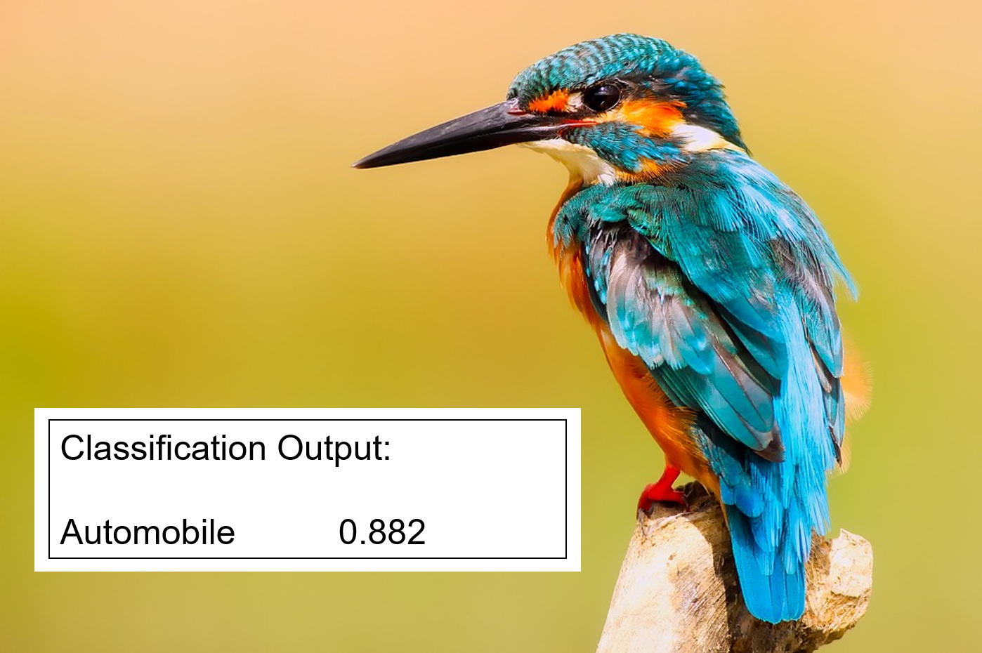
Figure 1. An example input to & output from a ML based image classifier. The classification is clearly wrong from a human-oracle expectation. Problem definition: Software verification should be able to ascertain that a) the classification is correct as per the specification (i.e. for the given training data, the classification for the example is correct); b) score of 0.882 for the class is correct. Image source: (pixabay, [n. d.])

The current options for a tester to test ML applications is largely left to validation. The tester would acquire a large number of real-life inputs and check that the outputs meet the expectation (with the tester acting as the human oracle). Such validation based testing would be very expensive in terms of time and cost.

When a ML algorithm exhibits an incorrect output (e.g. wrong classification to a particular input), there can be multiple underlying reasons. These include - a) deficient (e.g. biased) training data; b) poor ML architecture used; c) the ML algorithm learnt a wrong function; or d) there is an implementation bug. In the current state of practice, almost always an incorrect output is attributed to deficient training data and the developers would be urged to collect more diverse training data. However, we believe, the first aspect to ascertain is that the ML algorithm does not have implementation bugs. For example, if the fault that was seen is due to an implementation issue, getting more training data will not help.

‘Metamorphic Testing’ (Chen et al., 1998) is a prominent approach to test an ML application. Here, a test case has two tuples of ($\textrm{input}_{1}-\textrm{output}_{1}$) and ($\textrm{input}_{2}-\textrm{output}_{2}$). The second input, $\textrm{input}_{2}$, is created such that we can reason about the relation between $\textrm{output}_{1}$ and $\textrm{output}_{2}$. This relation between the outputs is termed as a Metamorphic Relation (MR). When we spot cases where the relation is not maintained, we can conclude that there is a bug in the implementation.

In this paper, we show how a tester can efficiently (with one or a few test cases) identify implementation issues in ML applications. Our approach is based on the concept of Metamorphic Testing and we have worked with two publicly available ML applications for image classification. The first application uses a Support Vector Machine (SVM) with options of a linear or a non-linear kernel. The second application is a deep learning based image classifier using a recent advancement in Convolutional Neural Networks, called a Residual Network (ResNet). For both the applications, we have developed metamorphic relations (MRs) and we provide justifications with proofs (where applicable), examples and empirical validation.

Our solution approach was validated through the concept of Mutation Testing (Jia and Harman, 2011). Bugs were artificially introduced into the two ML applications and we checked how many of these bugs could be caught through our technique. The tests showed that 71% of the implementation bugs were caught through our approach.

Our work advances the research in Metamorphic Testing in multiple ways: (i) we investigate the case of an SVM with a non-linear kernel, which hasn’t been done before, and we develop a new metamorphic relation (MR) for the linear-kernel; (ii) our work is the first to provide formal proofs of the MRs based on the mathematical formulation of SVM; (iii) we also develop MRs for the verification of a deep learning based image classifier, which is the first such work; and (iv) we evaluate the goodness of our approach through rigorous experiments and all of our data, results & code are open-sourced .

We anticipate our approach to be used by a tester as follows: when a ML based application is submitted to his/her desk for testing, the first step of verification can be done in an automated fashion through our approach. The tester would select relevant metamorphic relations and a tool based on our approach would automatically create test cases to check for the properties. If any of the properties do not hold, the verification has identified an implementation bug in the ML application.

This paper is structured as follows. We present the related work in Section 2. Section 3 presents our approach for two ML based image classifiers. Section 4 details the experimental results and we conclude in Section 5.

2. Related Work

Typical testing activity includes building tuples of (input-expected output). However, in many cases, the expected output cannot be ascertained easily (Xie et al., 2011). Examples include scientific programs which implement complex algorithms, programs which try to predict answers where the correct answer is not known (e.g., a program trying to predict the weather (Murphy and Kaiser, 2008)). Such programs have been termed as ‘non-testable programs’ (Weyuker, 1982) and machine learning algorithms are considered to be in this class.

Various methods have been devised to test ‘non-testable programs’. These include constructing an oracle from formal specification (Barr et al., 2015) (and recently formal verification has been attempted for machine learning (Selsam et al., 2017)), developing a pseudo oracle (or multiple implementations of a program (Srisakaokul et al., 2018)), testing on benchmark data (Karpathy, 2016), assertion checking (Murphy et al., 2009), using earlier versions of the program, developing trivial test cases where the oracle is easily obtainable (Murphy and Kaiser, 2010), using implicit oracles (such as when a program crashes) and Metamorphic Testing (Chen et al., 1998). While none of these methods have been found to solve all aspects (Barr et al., 2015), Metamorphic Testing has been found to be quite useful (Liu et al., 2014). We refer the readers to a recent survey (Barr et al., 2015) for a discussion on these various methods.

There has been work in the application of Metamorphic Testing over machine learning algorithms. This includes the testing of Naive-Bayes classifier (Xie et al., 2009)(Xie et al., 2011), support vector machine with a linear kernel (Murphy and Kaiser, 2010) and k-nearest neighbor (Xie et al., 2009) (Xie et al., 2011). However, none of these works investigate the case of an SVM with non-linear kernel (which is commonly used). Our work also applies metamorphic testing on deep learning based classifiers.

A recent work on applying Metamorphic Testing to test deep learning frameworks has been made (Ding et al., 2017). However, this work attempts to perform ‘validation’ and develops MRs based on the typical expectations from deep learning. For example, the first MR developed in (Ding et al., 2017) claims that the classification accuracy of a deep learning architecture should be better than a SVM. Further, the work in (Ding et al., 2017) does not provide justifications for the relations and does not perform an empirical validation.

Another recent work in the verification of ML is the use of formal methods (Selsam et al., 2017). This work has developed a mathematical language and an associated tool (called Certigrad) where a developer can specify the ML algorithm and verify the implementation using an interactive proof assistant. However, a key challenge of this method is the scalability to support a wide range of machine learning methods, the need for developers to learn a new formal language and the inability to check whether the specification written in the formal language is correct. Nevertheless, this work recognizes the difficulty of verifying machine learning algorithms and focuses on the case of identifying implementation bugs (which our work does as well).

Finally, some recent work has been made to specifically identify failure cases in deep learning architectures (Tian et al., 2017) (Pei et al., 2017). These works aim to ‘validate’ a deep learning system by building test inputs reflecting real-world cases. The focus of such work is in the identification of deficiencies in training data, or using a poor learning algorithm. Similar work is done by the entire area of adversarial examples (Papernot et al., 2016). In contrast, our work specifically investigates the case of ‘verification’ where the underlying root cause for a fault is an implementation bug.

3. Identifying Implementation Bugs in ML based applications

In this section, we will present our solution methodology. We have designed the metamorphic properties and validated our approach on the following publicly available ML based applications.

• Hand-written digit recognition from images using SVM with a linear and a non-linear kernel (Scikit-Learn, [n. d.])

• Image classification using Residual Networks (a type of Deep Convolutional Neural Network) (TensorFlow, [n. d.])

3.1. Metamorphic Relations for Application 1: Digit Recognition using SVM

We selected an application (Scikit-Learn, [n. d.]) that classifies images of hand written digits into classes of $0$ to $9$. The application is an official implementation from Scikit-learn, a popular machine learning library and uses a Support Vector Machine (SVM) for the classification. The application can be configured to use either a linear kernel or a non-linear kernel. We have developed metamorphic relations for both configurations with the non-linear kernel being an RBF kernel.

For training, the SVM application takes labeled examples of hand-written digits and learns decision boundaries separating the classes. Each example is an image of 8 pixels by 8 pixels. The pixels are in gray-scale and one example is represented by an array of 64 numbers. See Figure 2(a) for visualization of some of the examples.

For testing, the application takes an example and predicts the class (between ‘0’ & ‘9’). The application also provides a score depicting its confidence on the classification. The score is the (functional) distance of the example from the decision boundary - a large score means the example is farther away from the decision boundary and the classifier is more certain of its decision.

We have developed the following metamorphic relations (MRs):

1. MR-1: Permutation of training & test features

2. MR-2: Permutation of order of training instances

3. MR-3: Shifting of training & test features by a constant (only for RBF kernel)

4. MR-4: Linear scaling of the test features (only for linear kernel)

To justify the validity of the MRs, we will provide proofs based on the formulation of the SVM algorithm.

The SVM application uses the formulation of the LIBSVM (Chang and Lin, 2011) library. The formulation can be represented in primal form and in a corresponding dual form. The optimization is done, by default, in the dual form and our proofs are also based on this form.

Let the training dataset be represented by $(x_{i},y_{i})$, $i=1,...,m$, $x_{i}\in R^{n}$, $y_{i}\in\{-1,+1\}$. $x_{i}$ denotes one hand-written image and $y_{i}$ is its label. LIBSVM solves the following constrained optimization problem to find the optimal value of $\alpha$ (this is the dual form).

(1) $$\underset{\alpha}{\text{minimize}} \frac{1}{2}{\alpha}^{T}Q\alpha-{e}^{T}\alpha$$

subject to $$y^{T}\alpha=0,0\leq{\alpha}_{i}\leq C,\forall i=1\ldots m$$

Here, Q is a square matrix whose each element (i, j) is defined as: $Q_{ij}=y_{i}y_{j}K(x_{i},x_{j})$. The function $K(x_{i},x_{j})$ is the kernel. Once the optimization is complete, given a test instance $x_{a}$, the functional distance of the instance from the decision boundary is given by Equation (2). The class is $1$ if the functional distance is $\geq 0$ else $-1$.

(2) $$D(x_{a})=\sum_{i=1}^{i=m}\alpha_{i}y_{i}K(x_{a},x_{i})+b$$

For the linear kernel, we have $K(x_{i},x_{j})=x_{i}^{T}x_{j}$ (i.e. the dot-product between the data instances $x_{i}$ and $x_{j}$). For the RBF kernel we have $K(x_{i},x_{j})=e^{-\gamma||x_{i}-x_{j}||^{2}}$ (i.e. a measure of the distance between the two data instances $x_{i}$ and $x_{j}$).

Note that the formulation of SVM in dual form is completely expressed by the kernel function $K(x_{i},x_{j})$. This forms the underlying principle of our proofs where we show that transforming $x_{i}$ and $x_{j}$ in a particular way will lead to the transformation of the kernel $K(x_{i},x_{j})$ in a known and decidable way.

3.1.1. MR-1: Permutation of Training & Test Features

Let $X_{train}$ be the set of training data and $X_{test}$ be the set of test data. Upon completion of training via SVM, let a particular test instance, $x_{test}^{i}$ be classified as class $c$ with a score of $s$. MR-1 specifies that if we re-order the features of $X_{train}$ and $X_{test}$ through a deterministic function, say $perm()$, and re-train the SVM with $perm(X_{train})$, then the test instance $perm(x_{test}^{i})$ will continue to be classified as class $c$ with the same score of $s$.

To give an example of the function $perm()$, consider two data instances $x_{a}=(x_{1}^{a},x_{2}^{a},x_{3}^{a})$ and $x_{b}=(x_{1}^{b},x_{2}^{b},x_{3}^{b})$. The function $perm()$ re-orders the features as follows: $x_{a}^{p}=(x_{2}^{a},x_{3}^{a},x_{1}^{a})$ and $x_{b}^{p}=(x_{2}^{b},x_{3}^{b},x_{1}^{b})$ (note that both the instances are permuted in the same way). The feature permutation is visualized in Figure 2.

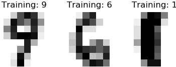
(a) Original training data

(b) Original test data

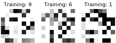
(c) Permuted training data

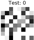
(d) Permuted test data

Figure 2. Visualization of MR-1. The results would be the same whether the SVM is trained & tested on the original or permuted data.

Proof.

Consider the examples $x_{a}$ and $x_{b}$ and their permuted versions $x_{a}^{p}$ and $x_{b}^{p}$. From Equation (1), the impact of the permutation is in the kernel function $K(x_{a},x_{b})$. For the linear kernel we have $K(x_{a},x_{b})={x_{a}}^{T}{x_{b}}=x_{1}^{a}x_{1}^{b}+x_{2}^{a}x_{2}^{b}+x_{3}^{a}x_{3}^{b}$. Further, $K(x_{a}^{p},x_{b}^{p})={x_{a}^{p}}^{T}{x_{b}^{p}}=x_{2}^{a}x_{2}^{b}+x_{3}^{a}x_{3}^{b}+x_{1}^{a}x_{1}^{b}=K(x_{a},x_{b})$.

Similarly, for the RBF kernel we have:

$K(x_{a},x_{b})=e^{-\gamma((x_{1}^{a}-x_{1}^{b})^{2}+(x_{2}^{a}-x_{2}^{b})^{2}+(x_{3}^{a}-x_{3}^{b})^{2})}$. Further, $K(x_{a}^{p},x_{b}^{p})=e^{-\gamma((x_{2}^{a}-x_{2}^{b})^{2}+(x_{3}^{a}-x_{3}^{b})^{2}+(x_{1}^{a}-x_{1}^{b})^{2})}=K(x_{a},x_{b})$. ∎

3.1.2. MR-2: Permutation of Order of Training Instances

Let $X_{train}$ be the set of training data. This MR specifies that if we shuffle $X_{train}$ (i.e. change the order of the individual examples), the results would not change. This is evident from Equation (1) where re-ordering the training instances, re-orders the constraints. However, the optimization is done to satisfy all the constraints and therefore the constraints’ order will make no difference.

3.1.3. MR-3: Shifting of Training & Test Features by a Constant (only for RBF Kernel)

Let $X_{train}$ be the training data & $X_{test}$ be the test data. Upon training via SVM, let a particular test instance, $x_{test}^{i}$ be classified as class $c$ with a score of $s$. MR-3 specifies that if we add a constant $k$ to each feature of $X_{train}$ & $X_{test}$, the re-trained SVM will continue to classify $x_{test}^{i}$ as class $c$ with score $s$.

Proof.

Consider the examples $x_{a}=(x_{1}^{a},x_{2}^{a},x_{3}^{a})$, $x_{b}=(x_{1}^{b},x_{2}^{b},x_{3}^{b})$ and their shifted versions $x_{a}^{s}=(x_{1}^{a}+k,x_{2}^{a}+k,x_{3}^{a}+k)$ and $x_{b}^{s}=(x_{1}^{b}+k,x_{2}^{b}+k,x_{3}^{b}+k)$. For the RBF kernel we have,

$K(x_{a}^{s},x_{b}^{s})=e^{-\gamma((x_{1}^{a}+k-(x_{1}^{b}+k))^{2}+(x_{2}^{a}+k-(x_{2}^{b}+k))^{2}+(x_{3}^{a}-(x_{3}^{b}+k))^{2})}=K(x_{a},x_{b})$. ∎

3.1.4. MR-4: Linear Scaling of the Test Features (only for Linear Kernel)

Let $X_{train}$ be the set of training data and $X_{test}$ be the set of test data. Upon completion of training via SVM, let a particular test instance, $x_{a}$ be classified as class $c$ with a score of $s$. For this MR, we scale only the test instances as follows. Let $x_{b}=2*x_{a}$ and $x_{c}=3*x_{a}$. Then, the functional distance between $x_{a}$ and $x_{b}$ would be equal to the functional distance between $x_{b}$ and $x_{c}$. Note that the classes of $x_{b}$ and $x_{c}$ need not be $c$. This MR can be used on an already trained model and thus in cases where the training API is not available to the tester.

Proof.

Since the optimization has already been completed, the optimal values of $\alpha$ have been found through Equation (1). Using Equation (2), we can reason about the functional distances:

$$D(x_{b})-D(x_{a}) =\sum_{i=1}^{i=m}\alpha_{i}y_{i}K(x_{b},x_{i})+b-\sum_{i=1}^{i=m}\alpha_{i}y_{i}K(x_{a},x_{i})-b$$

$$=2\sum_{i=1}^{i=m}\alpha_{i}y_{i}{x_{a}}^{T}{x_{i}}-\sum_{i=1}^{i=m}\alpha_{i}y_{i}{x_{a}}^{T}{x_{i}}$$

$$\text{Since }x_{b}=2*x_{a}\text{ and }{(2x)}^{T}x=2*{(x)}^{T}x$$

$$=\sum_{i=1}^{i=m}\alpha_{i}y_{i}{x_{a}}^{T}{x_{i}}$$

Similarly,

$$D(x_{c})-D(x_{b}) =3\sum_{i=1}^{i=m}\alpha_{i}y_{i}{x_{a}}^{T}{x_{i}}-2\sum_{i=1}^{i=m}\alpha_{i}y_{i}{x_{a}}^{T}{x_{i}}$$

$$=\sum_{i=1}^{i=m}\alpha_{i}y_{i}{x_{a}}^{T}{x_{i}}=D(x_{b})-D(x_{a})$$

∎

Each of the four MRs developed, can have multiple variants. For example, in MR-1, the features can be permuted in multiple ways. However, since the outputs from the MRs are expected to be an exact match (within a threshold of $10^{-6}$), we created only one variant for each MR. The variant, however, ensured that every aspect of the data instance was changed. For example, in MR-1, every feature was permuted and in MR-2, the order of every training data instance was changed. Similarly, for MR-3 & MR-4, a single variant was used.

The efficacy of these MRs in terms of the potential to catch implementation bugs is presented in Section 4.

3.2. Metamorphic Relations for Application 2: Image Classification using ResNet

The second application, we have chosen, is a deep learning based image classifier called a Residual Network (ResNet) (He et al., 2016). The application classifies color images into $10$ classes. ResNet is considered as a breakthrough advancement in the usage of Convolutional Neural Networks (CNN) for image classification and has been shown to work very well (it won multiple competitions in image classification tasks in 2015 (Russakovsky et al., 2015) (Lin et al., 2014)). The ResNet architecture has also been shown to work well in different contexts (He et al., 2016) and is now being largely considered as a default choice for image classification (Karpathy, 2016).

We have taken the official implementation of ResNet in TensorFlow (TensorFlow, [n. d.]) (in particular the ResNet-32 configuration). The ResNet architecture comprises of a series of neural network layers and a simplified version is shown in Figure 3. The architecture consists of an initial Conv layer followed by a series of ‘blocks’. Each block consists of a Batch-Norm layer, the activation function of ReLU and another Conv layer. Between each block is a ‘skip’ connection (the skip connection is thought of as the breakthrough idea (TensorFlow, [n. d.])). Conceptually, the ResNet application is learning a complex, non-linear function, $f(X,W)$, where $X$ is the input data and $W$ is a set of weights.

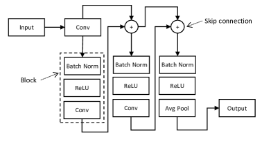
Figure 3. A simplified version of the ResNet Architecture.

The ResNet application trains and tests over the annotated data instances from the CIFAR-10 corpus (Krizhevsky et al., [n. d.]). Each data instance is a 32 by 32 pixel color image - i.e. each instance has 32 x 32 x 3 features (numbers) and has been categorized into 10 mutually exclusive classes. A few data instances are visualized in Figure 4. For a given set of test instances, the ResNet application predicts the classes and outputs the test classification accuracy and the ‘test loss’. The test loss (which is computed as the ‘cross-entropy’ between the actual class and the predicted class) is a measure of the goodness of the classification. This is analogous to the ‘score’ in SVM.

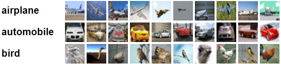
Figure 4. A sample of the training data of 3 classes.

We have developed the following metamorphic relations for the ResNet application.

1. MR-1: Permutation of input channels (i.e. RGB channels) for training and test data

2. MR-2: Permutation of the Convolution operation order for training and test data

3. MR-3: Normalizing the test data

4. MR-4: Scaling the test data by a constant

3.2.1. MR-1: Permutation of Input Channels (i.e. RGB Channels)

The RGB channels of an image hold the pixel values for the ‘red’, ‘green’ and ‘blue’ colors. This data is typically represented in a fixed order of R, G and B. For example, in the CIFAR-10 data, the first 1024 bytes are the values of the R channel, the next 1024 bytes are the values of the G channel, finally followed by 1024 bytes of the B channel. In total, the 3072 bytes forms the data for one image.

Let $X_{train}$ denote the training dataset and $X_{test}$ denote the set of test data. Given this original data, let the ResNet application complete training and output a test loss and accuracy. The MR claims, if the RGB channels of both $X_{train}$ and $X_{test}$ are permuted (for example, the permutation can be: the first 1024 bytes of the data would contain the B channel, followed by 1024 bytes of the G channel, ending with 1024 bytes of the R channel), a correctly implemented ResNet application should still be able to learn the same (or very similar) set of weights and therefore output the same (or very similar) test loss and accuracy.

This MR is similar, in principle, with the MR-1 of the SVM application (permutation of features). However, in the case of ResNet, we cannot do any arbitrary permutation - for example, we cannot permute pixel 1 with pixel 20 and vice-versa (as was done in the case of SVM). This is because, the CNN layer is built to exploit the ‘locality of pixel dependencies’ of an image - where groups of pixels close to each other tend to carry similar semantics (Krizhevsky et al., 2012). Thus, the MR-1 (and MR-2 as we will see later) make specific permutations such that this locality property is not violated.

The RGB channels can be permuted in $6$ ways, one of which is the original data (RGB channel in order). We use all 6 variants for this metamorphic relation. The variants are visualized in Figure 5.

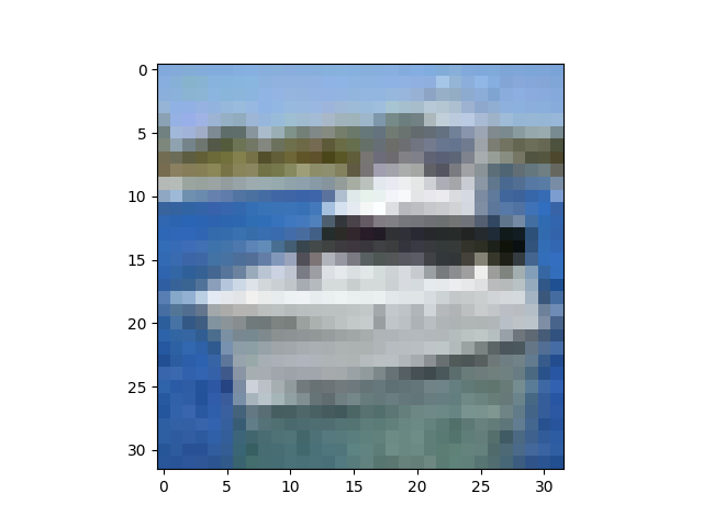
(a) Original training data (RGB)

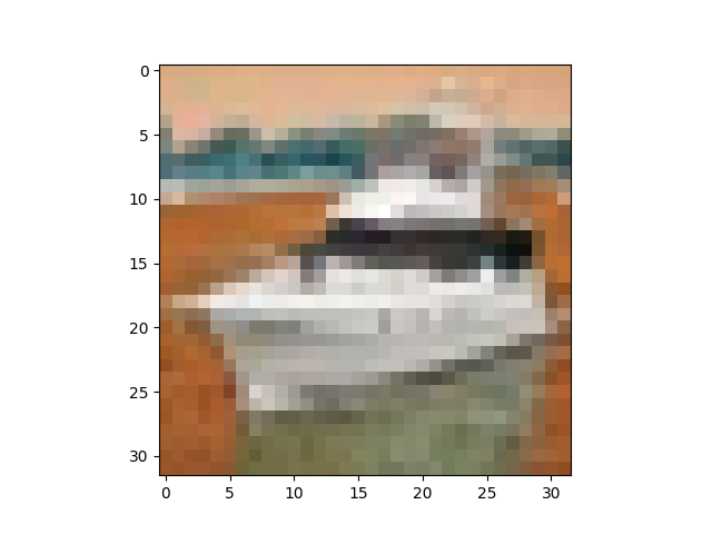
(b) BGR

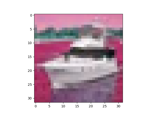
(c) BRG

(d) GBR

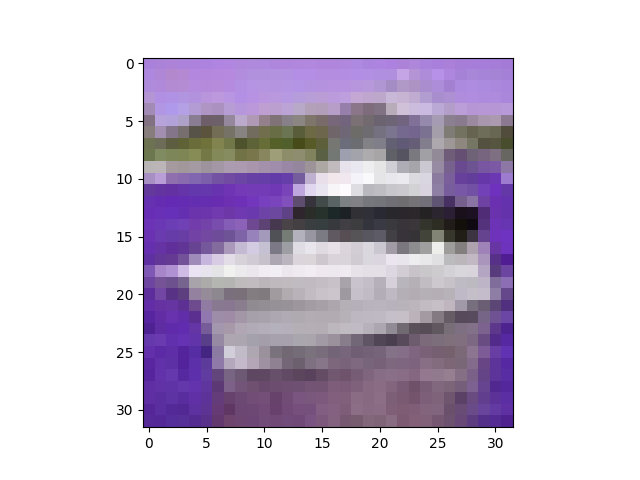
(e) GRB

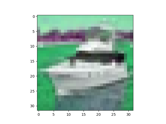
(f) RBG

Figure 5. Permutation of RGB channels for one instance of training data. The test data is permuted in similar fashion. The results should be very similar whether the ResNet application is trained & tested on the original or permuted data.

Reasoning.

The validity of the MR can be explained in two steps. In the first, we will show that the core property of a CNN (i.e. the ‘locality property’) is not violated by the RGB permutation. This is done by showing that the set of weights which were found while training on the original data is a valid solution on the permuted data. However, we cannot claim that this same set of weights will be found by the optimization method (unlike in the case of SVM). Thus, in the second step, we will show through some empirical results (both ours and those from existing literature) that in practice, a set of weights very close to the original is found.

The first CNN layer of ResNet architecture (refer Figure 3) has a weight for each of the three channels. Consider the first pixel of an image, which can be represented as $I=[i^{r},i^{g},i^{b}]$. Similarly, let the first weight of the CNN layer be represented as $W=[w^{r},w^{g},w^{b}]$. Then the convolution operation gives the result: $CONV(I,W)=i^{r}w^{r}+i^{g}w^{g}+i^{b}w^{b}$.

Now, let the permuted input and weight be: $I^{p}=[i^{b},i^{g},i^{r}]\&W^{p}=[w^{b},w^{g},w^{r}]$. Then, $CONV(I^{p},W^{p})=i^{b}w^{b}+i^{g}w^{g}+i^{r}w^{r}=CONV(I,W)$. Thus, the output from the first layer would be the same as before, and this implies all subsequent outputs (including the final classification) would be the same as before. The maintenance of the locality property can also be seen in Figure 5 where the images are still semantically recognizable.

However, it isn’t clear whether the optimization method used in the ResNet application (which is based on gradient descent) can indeed arrive at the set of weights $W^{p}$. At the start of training, the weights of the model (the parameters) are initialized to some random values. The weights are then changed as per the gradient of the loss ($L$) w.r.t the weights ($\frac{\partial}{\partial w}L$). Changing the input data from RGB to BGR makes no difference to the initialization of the weights, however, the gradient changes with the change in input. This means that the weights start from the same point in the weight space for RGB and BGR, but start moving in different directions and can converge at different points (i.e. the error surfaces are different for RGB & BGR).

The impact of change of channels can be conceptualized in another way. Instead of thinking of changing error surfaces, we can instead consider the impact of changing RGB to BGR as though the initialization of the weights for BGR is in a different point in the error surface of the RGB data. Thus, changing channels essentially means changing the initialization points and this can lead to different convergence. However recent empirical evidence (Goodfellow et al., 2014) (Choromanska et al., 2015) (Dauphin et al., 2014) suggests that practically, these different convergence points are very close to each other in terms of overall loss. Thus, it is expected that irrespective of the change in input from RGB to BGR, the weights to which they converge, must be very close to each other in terms of the overall loss. ∎

Empirical Evidence.

To give further credence to this MR, we conducted a set of empirical tests. We selected three additional datasets and three different architectures (shown in Table 1) to validate the MR. The variation in loss (on the test data) for the experiments as the training progresses is shown in Figure 6. Due to space considerations, we show the results on two datasets and two architectures. Complete data is available in Appendix A (Dwarakanath et al., 2018). Notice that there is little variation in the curves for the RGB variants and this is also measured as the maximum of the standard deviation ($\sigma_{max}$) in Table 1.

The combination of the tests showed that permuting the order of the RGB channels does not significantly change the results. From Table 1, we can also observe that this property holds for different architectures and different datasets.∎

Table 1. Experiments conducted to validate MR-1 & MR-2

Deep Learning Architecture	Dataset	$\sigma_{max}$ in test loss due to MR-1 (permute RGB)	$\sigma_{max}$ in test loss due to MR-2 (permute CONV order)
ResNet	Cifar10	4.8	3.6
ResNet	SVHN (Netzer et al., 2011)	1.4	3.3
ResNet	Kaggle Fruits (Oltean, 2018)	0.8	2.1
ResNet	Kaggle digits (Belitskaya, 2018)	1.1	0.9
AlexNet (Krizhevsky et al., 2012)	Cifar10	0.3	0.3
VGGNet (Simonyan and Zisserman, 2014)	Cifar10	0.1	0.1
NIN (Lin et al., 2013)	Cifar10	0.2	0.2

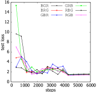
(a) MR-1 on ResNet code with CIFAR10 data

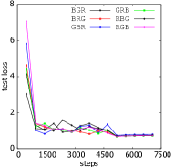
(b) MR-1 on ResNet code with SVHN data

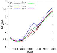
(c) MR-1 on AlexNet code with CIFAR10 data

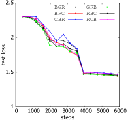
(d) MR-1 on VGGNet code with CIFAR10 data

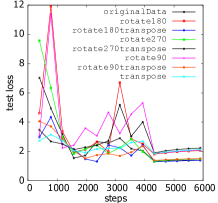
(e) MR-2 on ResNet code with CIFAR10 data

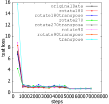
(f) MR-2 on ResNet code with SVHN data

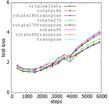
(g) MR-2 on AlexNet code with CIFAR10 data

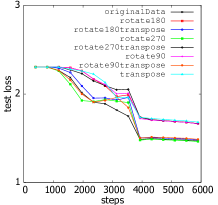
(h) MR-2 on VGGNet code with CIFAR10 data

Figure 6. Test loss from original code (non-buggy) due to changes in RGB order per MR-1 (top four graphs) and permuting input per MR-2 (bottom four graphs) for different datasets & architectures. Please see Appendix A (Dwarakanath et al., 2018) for complete results.

3.2.2. MR-2: Permutation of the Convolution Operation Order for Training and Test Data

This MR, again, is similar to the case of permutation of features for SVM (Section 3.1.1). However, we need to explicitly maintain the locality property of the permuted features. Our metamorphic relation, is to permute the input pixels such that the local neighborhood is maintained - i.e pixels which were neighbors in the original image, continue to be neighbors in the permuted image. To explain this, consider an image $I$ with pixel values as shown in Figure 7. $I$ contains 3 x 3 pixels and $I^{T}$ represents a permutation of the image such that the neighbors of every pixel are maintained. The permutation shown is a matrix transpose.

$$I=\begin{bmatrix}1&2&3\\ 4&5&6\\ 7&8&9\end{bmatrix}\ \ \ I^{T}=\begin{bmatrix}1&4&7\\ 2&5&8\\ 3&6&9\end{bmatrix}$$

Figure 7. An example image $I$ & it’s permutation $I^{T}$ which maintains the neighbors of every pixel

The MR is as follows. Let $X_{train}$ and $X_{test}$ be the training and test data respectively. After training the ResNet application with this data, let a instance of the test data $x_{test}^{i}$ be classified as class $c$ with a loss of $s$. If we permute the training and test data such that the neighborhood property is maintained and retrain the ResNet application on the permuted data, the (permuted) test instance will continue to be classified as class $c$ with a loss of $s$.

We have identified $7$ permutations that maintain the neighborhood property - matrix transpose, $90^{o}$ rotation, $180^{o}$ rotation, $270^{o}$ rotation & matrix transpose of each rotation. These $7$ transformations are visualized in Figure 8. We use these 7 variants along with the original image for MR-2.

(a) Original training data

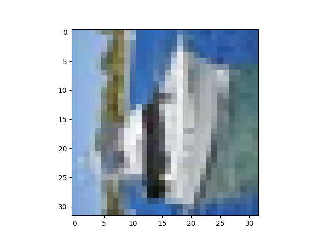
(b) Matrix Transform of original

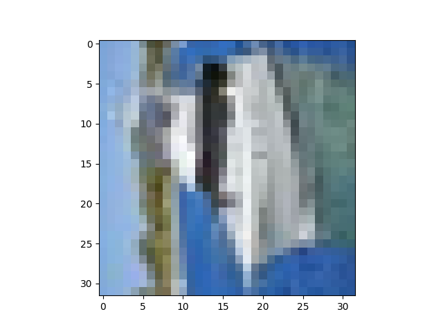
(c) $90^{o}$ rotation of original

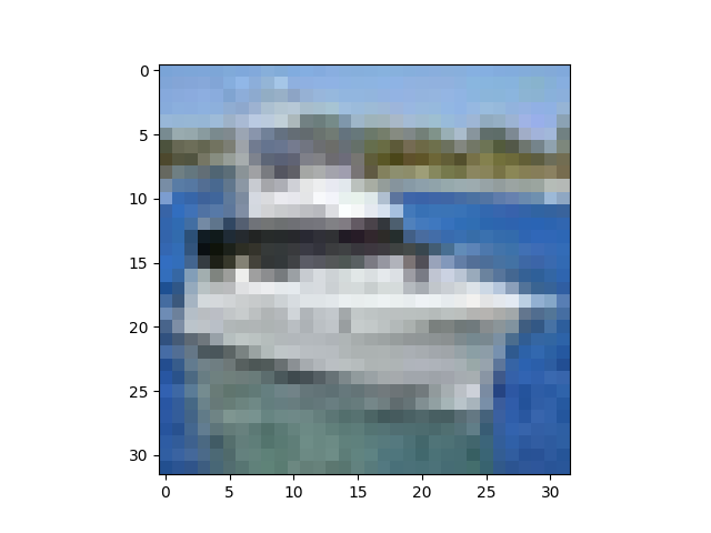
(d) Transform of $90^{o}$ rotation

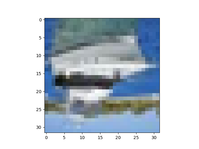
(e) $180^{o}$ rotation

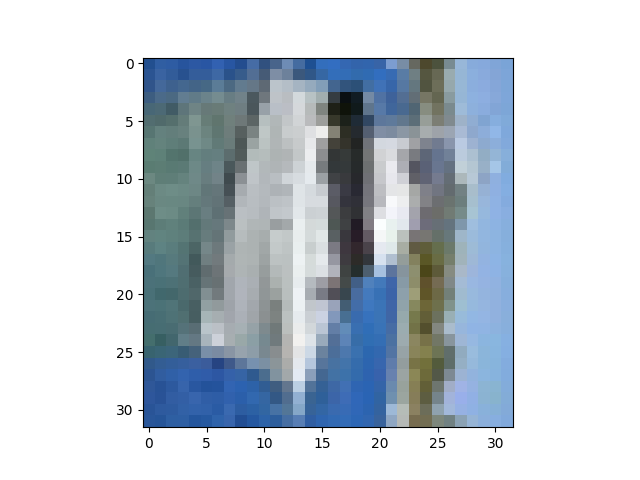
(f) Transform of $180^{o}$ rotation

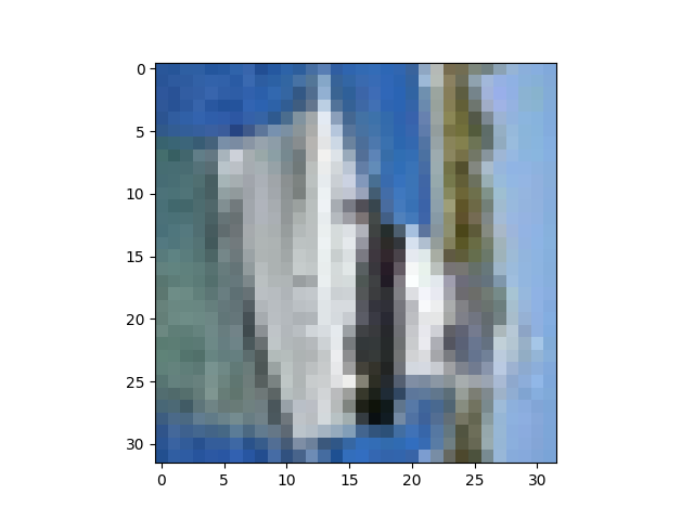
(g) $270^{o}$ rotation

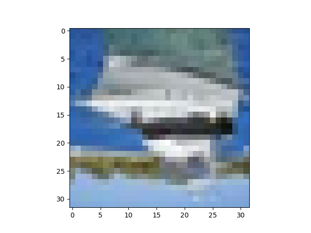
(h) Transform of $270^{o}$

Figure 8. Permutation of CONV order for one instance of training data. The test data is permuted in similar fashion

Reasoning.

The reasoning is similar to that of MR-1. Let the weight matrix of the first CONV layer (refer Figure 3) after training be $W$. Let $I$ be one test image. If we permute $I$ as $I^{T}$, and permute $W$ as $W^{T}$, then the output from the first CONV layer will be the same as before, except in permuted order. For example, consider an image $I$ and weight $W$ shown in Figure 9. We can see that $CONV(I,W)={CONV(I^{T},W^{T})}^{T}$. Thus, the output at each layer is a transpose of the earlier output. This property holds for all the layers in ResNet (including ReLU, BatchNorm and the skip connections). Thus, at the final layer, we would get the same output as before, but in transposed form. The weights at this final layer, again when transposed, will give the same classification and loss as before.

$$I=\begin{bmatrix}1&2&3\\ 1&1&2\\ 2&0&1\end{bmatrix}\ \ ,\ W=\begin{bmatrix}1&0\\ 2&3\end{bmatrix}\ \ ;\ CONV(I,W)=\begin{bmatrix}6&10\\ 5&4\end{bmatrix}$$

$$I^{T}=\begin{bmatrix}1&1&2\\ 2&1&0\\ 3&2&1\end{bmatrix}\ \ ,\ W^{T}=\begin{bmatrix}1&2\\ 0&3\end{bmatrix}\ \ ;\ CONV(I^{T},W^{T})=\begin{bmatrix}6&5\\ 10&4\end{bmatrix}$$

Figure 9. Example showing the impact of MR-2.

However, as in case of MR-1, we cannot claim that the optimization method will find the transposed set of weights. Nevertheless, the transposition of the input can be conceptualized as a different point in initialization and we can fallback on the empirical evidence which has shown that small changes in initialization do not significantly change the final convergence qualities. ∎

Empirical Evidence.

Similar to MR-1, we conducted empirical tests to validate MR-2. We took three different datasets and three different deep learning architectures. MR-2 (with 7 variants in the permutation of the inputs) was compared with the original data. Figure 6(e-h) shows the results. As before, we found the deviation of test loss after 150 epochs to be small. The deviation is captured as $\sigma_{max}$ in Table 1. ∎

A note on MR-1 & MR-2: It is a common practice to perform data-augmentation in ML applications. Data-augmentation includes cases such as mirroring images and some of the transformations in Figure 8 might look like cases of data-augmentation. However, our MRs are clearly distinct from data-augmentation. The intuition behind data-augmentation is that of ‘validation’ - i.e. a mirror-image is a naturally occurring phenomenon. Further, such mirror-images are computed and added to the training data where both the original and the mirror-image exist in the training data.

However, the transformation in our MRs is a case of ‘verification’. Some of the transformations may not naturally occur (many cases of RGB transformation look wrong to the naked eye). The MRs claim that the classification of an original image and the transformed image should lie in the same class (even if the class is wrong). Further, our transformations do not add to the training data - i.e. the transformed and the original image never co-exist in the training data.

3.2.3. MR-3: Normalizing the Test Data

A standard practice in machine learning applications is to normalize the training and test data. Normalization makes the data with a zero mean & unit variance (Karpathy, 2016) and leads to faster convergence.

Let $X_{train}$ be the training data and $x_{test}^{i}$ be one instance of the test data. Let the ResNet application complete its training on $X_{train}$. Let the classification of $x_{test}^{i}$ be $c$ with a loss of $s$. MR-3 specifies that if we normalize $x_{test}^{i}$ and feed this as the input the results would be exactly the same. This is visualized in Figure 10. Note that this MR needs only the test data to be normalized and therefore can be used to test already trained ML models.

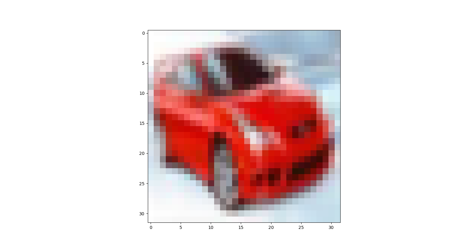
(a) Original test image

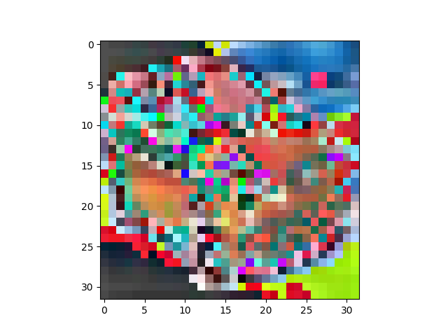
(b) Normalized test image

Figure 10. Visualisation of MR-3. The class & loss should be the same when tested on the original or normalized images.

Proof.

There are two forms of normalization that can be performed. In one, the normalization is done on the entire training data (or a minibatch). In the second form (as is done in ResNet), the normalization is done on individual data points. The proof below is for the latter version.

Let $x$ be a test image (an array of 32 x 32 x 3 numbers). The ResNet application first normalizes this data point (as per Equation (3)) before trying to classify it.

(3) $$x^{\prime}=\frac{x-\mu(x)}{\sigma(x)}$$

Now, if we normalize $x$ before providing it to the ResNet application, the second normalization that is done inside the ResNet application will not make any difference (as shown in Equation (4)). Thus, the results should be the same whether we supply the original test input or the normalized test input.

(4) $$x^{\prime\prime}=\frac{x^{\prime}-\mu(x^{\prime})}{\sigma(x^{\prime})}\\ =x^{\prime}\ \ since\ \mu(x^{\prime})=0\ \&\ \sigma(x^{\prime})=1$$

∎

3.2.4. MR-4: Scaling the Test Data by a Constant

Let the ResNet application complete the training on the original training data $X_{train}$. Let $x_{test}^{i}$ be an instance of the test data which is classified into class $c$ with a loss of $s$. MR-4 specifies that if every feature of the test instance $x_{test}^{i}$ is multiplied by a positive constant, $k$ and re-tested, the classification will continue to be $c$ with loss $s$.

(a) Original test image

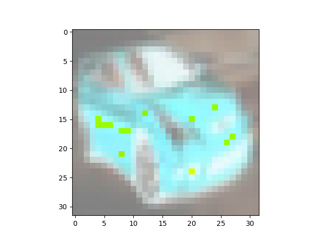
(b) $k=\frac{1}{2}$

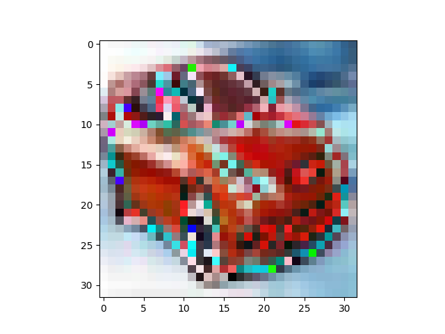
(c) $k=2$

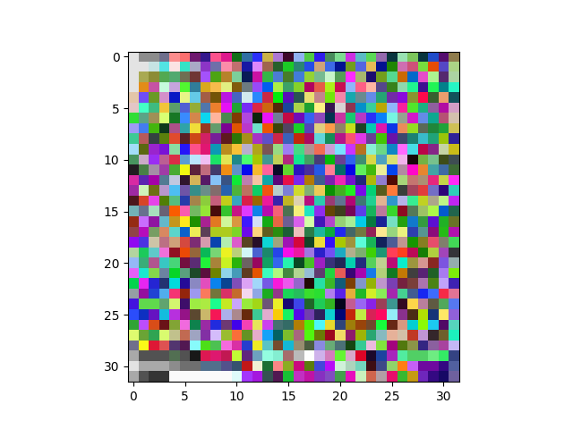
(d) $k=29$

Figure 11. Visualization of MR-4 (each feature is multiplied by a constant $k$). The class & loss should be the same when tested on the original or scaled images.

Proof.

Like MR-3, MR-4 is a consequence of the type of normalization used in ResNet. When every feature of the input image is multiplied by a constant, we have:

(5) $$\begin{split}x^{\prime}=\frac{kx-\mu(kx)}{\sigma(kx)}=\frac{k(x-\mu(x))}{k(\sigma(x))}=\frac{x-\mu(x)}{\sigma(x)}\\ \ \ since\ \mu(kx)=k\mu(x);\sigma(kx)=k\sigma(x)\end{split}$$

∎

Thus, the results should be same irrespective of the constant $k$. Like MR-3, this MR is applied only on the test data and therefore can be used to test already trained ML models.

MR-3 & MR-4 do not need an empirical validation as they are exact - i.e. any small deviations (we check for a variance $\geq 0.1$) in the outputs are sufficient to indicate the presence of a bug.

We now present the empirical results to validate the efficacy of the MRs developed.

4. Empirical Results

The efficacy of the MRs developed for the two ML applications was tested by purposefully introducing implementation bugs through the technique of Mutation Testing (Jia and Harman, 2011). Mutation testing systematically changes lines of code in the original source file and generates multiple new source code files. Each file will have exactly one bug introduced. Such a file with a bug is called a mutant. The principle underlying Mutation Testing is that the mutants generated represent the errors programmers typically make (Jia and Harman, 2011). This approach of using Mutation Testing to validate the efficacy of Metamorphic Testing has been used in the past as well(Xie et al., 2011)(Liu et al., 2014).

We used the MutPy tool (Foundation, 2013), from the Python Software Foundation, to generate the mutants. Each mutant was executed as per the MRs developed. If any of the results from the mutants did not adhere with what was specified by the MRs, we would term the mutant as ‘killed’ - i.e. the presence of a bug has been identified.

4.1. Results from Metamorphic Testing of Application 1

4.1.1. Creating the Mutants

The SVM application supports the linear kernel and the RBF (a non-linear) kernel. Using MutPy tool (Foundation, 2013), mutants for both variants were created. In total 52 mutants were generated for linear-SVM and 50 for RBF-SVM. Of these mutants, we removed those which throw a run-time exception or those which do not affect the program’s output (e.g., changes to the ‘print’ function). This resulted in 6 mutants of interest (the mutants were the same for both linear & rbf kernel). All the 6 mutants were of a similar kind and read the label of a data instance (which denotes the class) from a wrong column of the .csv data file. One of the mutants is shown in Figure 12.

   digits_target = digits[:,(-1)].astype(np.int)
ΨΨΨΨΨΨΨΨΨΨΨ
   digits_target = digits[:,1].astype(np.int)
Ψ

Figure 12. Original Code (top) and Mutant l2 (below). This mutant will read the wrong column of the data for the label.

4.1.2. Results

We took the training & test data available with the application and generated new datasets as per the MRs. Each of the 6 mutants was then executed with the original data and the new data. When the outputs (viz., class label and the distance of a data instance from the decision boundary) from the mutants did not match as per the MR, we report the mutant as killed. The results of running the MRs over the mutants are shown in Table 2.

The results show that all the six mutants of linear-SVM and RBF-SVM were caught through the MRs. In particular, MR-1 (permutation of input features) was sufficient to catch all the mutants. This is because, all the 6 mutants generated by the MutPy tool correspond to incorrect handling of input data (e.g., the mutant l2 as shown in Figure 12). MR-1 changed the input feature which caused the SVM to think the class label has changed and thus gave different outputs. For precisely the same reason, MR-3 (shifting the features by a constant) caught all the mutants as well.

Table 2. MRs applied on the mutants of linear-SVM & RBF-SVM. $\checkmark$ denotes the mutant was killed.

MR	Mutant Num of linear-SVM
	l2	l5	l8	l11	l22	l31
MR-1 (permute features)	✓	✓	✓	✓	✓	✓
MR-2 (re-order train instances)
MR-4 (scale test features)
	Mutant Num of RBF-SVM
	r2	r5	r8	r11	r22	r31
MR-1 (permute features)	✓	✓	✓	✓	✓	✓
MR-2 (re-order train instances)
MR-3 (shift train & test features)	✓	✓	✓	✓	✓	✓

4.2. Results from Metamorphic Testing of Application 2

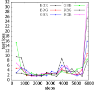
(a) MR-1 on Mutant c43

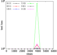
(b) MR-1 on Mutant c44

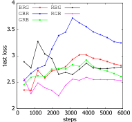
(c) MR-1 on Mutant c221

(d) MR-1 on Mutant c50

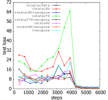
(e) MR-2 on Mutant c29

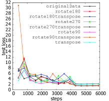
(f) MR-2 on Mutant c31

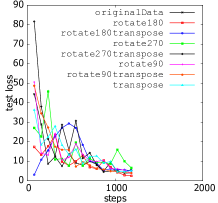
(g) MR-2 on Mutant c49

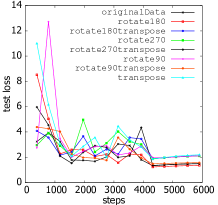
(h) MR-2 on Mutant r49

Figure 13. Test loss when mutants are run with MR-1 (top four graphs) and MR-2 (bottom four graphs). First three plots of each row are mutants that are caught. Clear outliers can be seen. Fourth plot of each row are mutants that were not caught. Please see Appendix B (Dwarakanath et al., 2018) for results for all mutants and for a discussion on why some were caught and others weren’t.

One of the challenges working with the ResNet application (and possibly deep neural networks) is the stochastic nature of the output where different results are seen for two runs with the same inputs. Such differing outputs is a challenge for Metamorphic Testing, as the MRs compare outputs of subsequent runs. We found stochasticity in the ResNet application to be due to the usage of random seeds. To alleviate this, we updated the code to use a fixed seed for each run. Fixing the seed made the application deterministic when run on a CPU, unfortunately, the application was still stochastic when executed on a GPU. Appendix C (Dwarakanath et al., 2018) provides details on the amount of variance seen on the GPU. We could not determine the cause for the non-determinism on the GPU, but it appears to be an issue with the NVidia CUDA libraries (jkschin, 2017) (antares1987, 2017). Thus, all our experiments were run on a CPU. Whether our results can be replicated on a GPU needs to be studied further.

The ResNet application trains by making multiple passes over the training data (called epochs). 150 epochs are made to complete the training. Completing 150 epochs of training on the entire CIFAR-10 data takes around 105 hours on an Intel i5 CPU. Therefore, we carefully selected $10\%$ of the CIFAR-10 data maintaining the data/class distribution. This resulted in 5,029 training and 1010 test instances. On this shortened data, 150 epochs of training takes approximately 10 hours. Our work in this paper has executed 392 experiments of 150 epochs (or 163 days of compute). The experiments were executed on Intel i5 CPU running Windows 10 with Tensorflow 1.7.

4.2.1. Creating the Mutants

The ResNet application code is written in two files - cifar10.py and resnet.py. Using MutPy tool (Foundation, 2013), mutants were created for both files. In total, $459$ mutants were created. We analyzed each mutant and discarded those that give a run-time exception, those that do not change the program’s output (because they are syntactic changes in code that is never reached) and those that were changes to the hyper-parameters (like the learning rate). This reduction led to 16 valid mutants . The types of valid mutants created is shown in Table 3. This gives an idea of the typical errors that may be created while writing deep learning applications in Python. Figure 14 shows a mutant of type ‘Change the loss function’.

Table 3. Types of Mutants created for ResNet application.

Mutant Type	Num. of Mutants
Reduce the training data files	3
Change the loss function	4
Changes to the learning rate decay	3
Interchange training and testing	2
Change the architecture of ResNet	2
Pad the wrong channels	2
Total	16

       loss = cross_entropy + _WEIGHT_DECAY
ΨΨΨΨΨΨΨΨΨΨΨ
       loss = cross_entropy - _WEIGHT_DECAY
Ψ

Figure 14. Original Code (top) and Mutant c29 (below). This mutant will explicitly attempt to overfit on the data.

4.2.2. Results

Figure 13 shows the plot of the test loss for a few mutants when run against MR-1 & MR-2. The plots capture the test loss that is output by the application after around every 300 steps of training. Plots of all mutants are available in Appendix B (Dwarakanath et al., 2018). From Figure 13, we can clearly see strong outliers for some of the mutants. However, we see no such outliers on the original (non-buggy) code (Figure 6) across datasets and architectures. To catch a mutant, we computed the standard deviation ($\sigma$) of the test loss at every step (across all variants of a MR) and considered the maximum deviation $\sigma_{max}$ across all steps. For example, $\sigma$ for MR-1 measures how deviant are the test losses of a mutant for all channel variants, RGB, BGR, etc., at a given step in training. For MR-1 & MR-2 we term the mutant as caught if this $\sigma_{max}$ is beyond a threshold (i.e. there is strong evidence that the variants of the MRs are not behaving alike). We used a threshold of 9 to report the results in Table 4, however, the results showed that the number of mutants killed would be same for any threshold between 5 to 9 (an indication of the large outliers seen in output of mutants). The test only MRs (MR-3 & MR-4) were also able to catch mutants. This is very useful since the MRs can be run very quickly since they work on an already trained model.

The MRs are not able to catch any of the r* mutants since all of them pertain to change in the architecture of the ResNet. For example, mutant r48 pads the depth channel of the image (thereby increasing the number of tunable parameters and increasing the capacity of the network). Such mutants on changes in architecture did not show any noticable change in the outputs. It would be extremely interesting to explore whether any MRs can indeed catch such mutants. For a discussion on why mutants are (not-)caught, please refer to Appendix B (Dwarakanath et al., 2018).

4.3. Discussion

Our experimental results show that the defined MRs for the SVM application is able to catch all of the 12 mutants (6 each for linear & RBF kernels) while the MRs defined for the ResNet application is able to catch 8 out of 16 mutants (for a total of 20/28 or 71%), which is promising. Metamorphic testing opens an interesting approach to test ML applications where one takes into account the characteristics of the datasets & the learning algorithm to define relations/properties that are expected to hold. This eases the burden on the testing team from creating large data sets for validation. Instead, the testing team can focus on generating generic metamorphic relations for a class of learning algorithms and datasets (e.g., for image classification, text analytics, etc.). Due to the computational complexity (long training times) of ResNet application, we selected a subset of data to validate our approach. It would make an interesting proposition to replicate the results on the full data set (although we expect to see a similar behavior). Furthermore, we would like to assess the strength of the defined MRs for other deep learning architectures.

Table 4. MRs applied on mutants of ResNet. Values in brackets report $\sigma_{max}$. In total 8 out of 16 (50%) of bugs were caught.

Mutant	MR-1 (permute RGB)	MR-2 (permute CONV order)	MR-3 (normalize data)	MR-4 (scale data)
c9
c29		✓(18.1)
c30
c31		✓(9.1)
c32		✓(9.1)
c43	✓(9.6)	✓(11.5)
c44	✓(27.4)	✓(9.2)
c45
c49	✓(23.3)	✓(23.8)		✓
c50			✓	✓
c116
c221	✓($\infty$)
r6
r48
r49
r67

5. Conclusion

In this paper we have investigated the problem of identifying implementation bugs in machine learning based applications. Current approaches to test an ML application is limited to ‘validation’, where the tester acts as a human-oracle. This is because ML applications are complex and verifying its output w.r.t the specification is extremely challenging. Our solution approach is based on the concept of Metamorphic Testing where we build multiple relations between subsequent outputs of a program to effectively reason about the correctness of the implementation. We have developed such relations for two image classification applications - one using a Support Vector Machine (SVM) classifier and another application using Deep Learning based Convolutional Neural Network. Experimental results showed that, on average, 71% of the implementation bugs were caught by our method and gives impetus for further exploration.

References

- (1)
- antares1987 (2017) antares1987. 2017. About Deterministic Behaviour of GPU implementation of tensorflow. https://github.com/tensorflow/tensorflow/issues/12871. [Online; accessed 15-Jan-2018].
- Barr et al. (2015) Earl T Barr, Mark Harman, Phil McMinn, Muzammil Shahbaz, and Shin Yoo. 2015. The oracle problem in software testing: A survey. IEEE transactions on software engineering 41, 5 (2015), 507–525.
- Belitskaya (2018) Olga Belitskaya. 2018. Handwritten Letters 2. https://www.kaggle.com/olgabelitskaya/handwritten-letters-2. [Online; accessed 12-Jan-2018].
- Chang and Lin (2011) Chih-Chung Chang and Chih-Jen Lin. 2011. LIBSVM: A library for support vector machines. ACM Transactions on Intelligent Systems and Technology 2 (2011), 27:1–27:27. Issue 3.
- Chen et al. (1998) Tsong Y Chen, Shing C Cheung, and Shiu Ming Yiu. 1998. Metamorphic testing: a new approach for generating next test cases. Technical Report. Technical Report HKUST-CS98-01, Department of Computer Science, Hong Kong University of Science and Technology, Hong Kong.
- Choromanska et al. (2015) Anna Choromanska, Mikael Henaff, Michael Mathieu, Gérard Ben Arous, and Yann LeCun. 2015. The loss surfaces of multilayer networks. In Artificial Intelligence and Statistics. 192–204.
- Dauphin et al. (2014) Yann N Dauphin, Razvan Pascanu, Caglar Gulcehre, Kyunghyun Cho, Surya Ganguli, and Yoshua Bengio. 2014. Identifying and attacking the saddle point problem in high-dimensional non-convex optimization. In Advances in neural information processing systems. 2933–2941.
- Ding et al. (2017) Junhua Ding, Xiaojun Kang, and Xin-Hua Hu. 2017. Validating a deep learning framework by metamorphic testing. In Proceedings of the 2nd International Workshop on Metamorphic Testing. IEEE Press, 28–34.
- Dwarakanath et al. (2018) Anurag Dwarakanath, Manish Ahuja, Samarth Sikand, Raghotham M Rao, Jagadeesh Chandra Bose R. P, Neville Dubash, and Sanjay Podder. 2018. Identifying Implementation Bugs in Machine Learning based Image Classifiers using Metamorphic Testing: Appendix. https://github.com/verml/VerifyML. [Online; accessed 2-May-2018].
- Foundation (2013) Python Software Foundation. 2013. MutPy 0.4.0. https://pypi.python.org/pypi/MutPy/0.4.0. [Online; accessed 15-Jan-2018].
- Goodfellow et al. (2014) Ian J. Goodfellow, Oriol Vinyals, and Andrew M. Saxe. 2014. Qualitatively characterizing neural network optimization problems. (2014). arXiv:1412.6544 http://arxiv.org/abs/1412.6544
- He et al. (2016) Kaiming He, Xiangyu Zhang, Shaoqing Ren, and Jian Sun. 2016. Deep residual learning for image recognition. In Proceedings of the IEEE conference on computer vision and pattern recognition. 770–778.
- IEEE ([n. d.]) IEEE. [n. d.]. IEEE Std 1012-2016 (Revision of IEEE Std 1012-2012/ Incorporates IEEE Std 1012-2016/Cor1-2017) - IEEE Standard for System, Software, and Hardware Verification and Validation. https://standards.ieee.org/findstds/standard/1012-2016.html. [Online; accessed 7-Jan-2018].
- Jia and Harman (2011) Yue Jia and Mark Harman. 2011. An analysis and survey of the development of mutation testing. IEEE transactions on software engineering 37, 5 (2011), 649–678.
- jkschin (2017) jkschin. 2017. Non-determinism Docs. https://github.com/tensorflow/tensorflow/pull/10636. [Online; accessed 15-Jan-2018].
- Karpathy (2016) Alex Karpathy. 2016. CS231n: Convolutional Neural Networks for Visual Recognition. http://cs231n.github.io/convolutional-networks/. [Online; accessed 26-Jan-2018].
- Krizhevsky et al. ([n. d.]) Alex Krizhevsky, Vinod Nair, and Geoffrey Hinton. [n. d.]. The CIFAR-10 dataset. https://www.cs.toronto.edu/~kriz/cifar.html. [Online; accessed 8-Sept-2017].
- Krizhevsky et al. (2012) Alex Krizhevsky, Ilya Sutskever, and Geoffrey E Hinton. 2012. Imagenet classification with deep convolutional neural networks. In Advances in neural information processing systems. 1097–1105.
- Lin et al. (2013) Min Lin, Qiang Chen, and Shuicheng Yan. 2013. Network in network. arXiv preprint arXiv:1312.4400 (2013).
- Lin et al. (2014) Tsung-Yi Lin, Michael Maire, Serge Belongie, James Hays, Pietro Perona, Deva Ramanan, Piotr Dollár, and C Lawrence Zitnick. 2014. Microsoft coco: Common objects in context. In European conference on computer vision. Springer, 740–755.
- Liu et al. (2014) Huai Liu, Fei-Ching Kuo, Dave Towey, and Tsong Yueh Chen. 2014. How effectively does metamorphic testing alleviate the oracle problem? IEEE Transactions on Software Engineering 40, 1 (2014), 4–22.
- Murphy and Kaiser (2010) Christian Murphy and Gail Kaiser. 2010. Empirical evaluation of approaches to testing applications without test oracles. Dep. of Computer Science, Columbia University, Tech. Rep. CUCS-039-09 (2010).
- Murphy and Kaiser (2008) Christian Murphy and Gail E Kaiser. 2008. Improving the dependability of machine learning applications. (2008).
- Murphy et al. (2009) Christian Murphy, Kuang Shen, and Gail Kaiser. 2009. Using JML runtime assertion checking to automate metamorphic testing in applications without test oracles. In Software Testing Verification and Validation, 2009. ICST’09. International Conference on. IEEE, 436–445.
- Netzer et al. (2011) Yuval Netzer, Tao Wang, Adam Coates, Alessandro Bissacco, Bo Wu, and Andrew Y Ng. 2011. Reading digits in natural images with unsupervised feature learning. In NIPS workshop on deep learning and unsupervised feature learning, Vol. 2011. 5.
- Oltean (2018) Mihai Oltean. 2018. Fruits 360 Dataset. https://www.kaggle.com/moltean/fruits/data. [Online; accessed 12-Jan-2018].
- Papernot et al. (2016) Nicolas Papernot, Patrick McDaniel, Ian Goodfellow, Somesh Jha, Z Berkay Celik, and Ananthram Swami. 2016. Practical black-box attacks against deep learning systems using adversarial examples. arXiv preprint arXiv:1602.02697 (2016).
- Pei et al. (2017) Kexin Pei, Yinzhi Cao, Junfeng Yang, and Suman Jana. 2017. DeepXplore: Automated Whitebox Testing of Deep Learning Systems. arXiv preprint arXiv:1705.06640 (2017).
- pixabay ([n. d.]) pixabay. [n. d.]. https://pixabay.com/en/photos/bird/. [Online; accessed 5-Sept-2017].
- Russakovsky et al. (2015) Olga Russakovsky, Jia Deng, Hao Su, Jonathan Krause, Sanjeev Satheesh, Sean Ma, Zhiheng Huang, Andrej Karpathy, Aditya Khosla, Michael Bernstein, Alexander C. Berg, and Li Fei-Fei. 2015. ImageNet Large Scale Visual Recognition Challenge. International Journal of Computer Vision (IJCV) 115, 3 (2015), 211–252. https://doi.org/10.1007/s11263-015-0816-y
- Scikit-Learn ([n. d.]) Scikit-Learn. [n. d.]. Scikit-learn example: Recognizing hand-written digits. http://scikit-learn.org/stable/auto_examples/classification/plot_digits_classification.html. [Online; accessed 6-Sept-2017].
- Selsam et al. (2017) Daniel Selsam, Percy Liang, and David L Dill. 2017. Developing Bug-Free Machine Learning Systems With Formal Mathematics. In International Conference on Machine Learning. 3047–3056.
- Simonyan and Zisserman (2014) Karen Simonyan and Andrew Zisserman. 2014. Very deep convolutional networks for large-scale image recognition. arXiv preprint arXiv:1409.1556 (2014).
- Srisakaokul et al. (2018) Siwakorn Srisakaokul, Zhengkai Wu, Angello Astorga, Oreoluwa Alebiosu, and Tao Xie. 2018. Multiple-Implementation Testing of Supervised Learning Software. (2018).
- TensorFlow ([n. d.]) TensorFlow. [n. d.]. ResNet in TensorFlow. https://github.com/tensorflow/models/tree/master/official/resnet. [Online; accessed 28-Dec-2017].
- Tian et al. (2017) Yuchi Tian, Kexin Pei, Suman Jana, and Baishakhi Ray. 2017. DeepTest: Automated testing of deep-neural-network-driven autonomous cars. arXiv preprint arXiv:1708.08559 (2017).
- Weyuker (1982) Elaine J Weyuker. 1982. On testing non-testable programs. Comput. J. 25, 4 (1982), 465–470.
- Xie et al. (2009) Xiaoyuan Xie, Joshua Ho, Christian Murphy, Gail Kaiser, Baowen Xu, and Tsong Yueh Chen. 2009. Application of metamorphic testing to supervised classifiers. In Quality Software, 2009. QSIC’09. 9th International Conference on. IEEE, 135–144.
- Xie et al. (2011) Xiaoyuan Xie, Joshua WK Ho, Christian Murphy, Gail Kaiser, Baowen Xu, and Tsong Yueh Chen. 2011. Testing and validating machine learning classifiers by metamorphic testing. Journal of Systems and Software 84, 4 (2011), 544–558.