Efficient Operator-Coarsening Multigrid Schemes for Local Discontinuous Galerkin Methods

Abstract

An efficient $hp$-multigrid scheme is presented for local discontinuous Galerkin (LDG) discretizations of elliptic problems, formulated around the idea of separately coarsening the underlying discrete gradient and divergence operators. We show that traditional multigrid coarsening of the primal formulation leads to poor and suboptimal multigrid performance, whereas coarsening of the flux formulation leads to optimal convergence and is equivalent to a purely geometric multigrid method. The resulting operator-coarsening schemes do not require the entire mesh hierarchy to be explicitly built, thereby obviating the need to compute quadrature rules, lifting operators, and other mesh-related quantities on coarse meshes. We show that good multigrid convergence rates are achieved in a variety of numerical tests on 2D and 3D uniform and adaptive Cartesian grids, as well as for curved domains using implicitly defined meshes and for multi-phase elliptic interface problems with complex geometry. Extension to non-LDG discretizations is briefly discussed.

65N55, 65N30, 65F08

1 Introduction

Discontinuous Galerkin (DG) methods have gained broad popularity in recent years. They are well-suited to $hp$-adaptivity, provide high-order accuracy, and can be applied to a wide range of problems on complex geometries with unstructured meshes. Although DG methods were first applied to the discretization of hyperbolic conservation laws, they have been extended to handle elliptic problems and diffusive operators in a unified framework [7]. Such methods include the symmetric interior penalty (SIP) method [21, 6], the Bassi–Rebay (BR1, BR2) methods [9, 10], the local discontinuous Galerkin (LDG) method [20], the compact discontinuous Galerkin (CDG) method [31], the line-based discontinuous Galerkin method [32], and the hybridizable discontinuous Galerkin (HDG) method [18]. In particular, the development of efficient solvers for DG discretizations of elliptic problems is an active area of research.

Among the panoply of DG methods for elliptic problems, the LDG method is a popular choice: it is accurate, stable, simple to implement, and extendable to higher-order derivatives [43]. Additionally, on Cartesian grids it has been shown to be superconvergent [19]. The LDG method results in symmetric positive (semi)definite discretizations which are well-suited to solution by efficient iterative methods. In particular, the multigrid method has emerged as a natural candidate due to its success in the continuous finite element and finite difference communities, both as a standalone solver and as a preconditioner for the conjugate gradient (PCG) method. However, direct application of standard multigrid techniques to DG discretizations of elliptic problems can result in suboptimal performance when inherited bilinear forms are employed [2, 24], and much work has gone into developing specialized smoothers and coarse-correction methods to remedy this issue, even on Cartesian grids [27, 22].

When a mesh hierarchy is available, geometric $h$-multigrid is a natural choice of solver. Error estimates have been derived for a multilevel interior penalty (IP) method on unstructured meshes, yielding convergence factors in the range $\rho\approx 0.3$–$0.5$ for Poisson’s equation [24, 12]; the method has also been applied to adaptively refined Cartesian grids with similar results [28]. Subsequent work describes how the multilevel IP method [24] can be used as a preconditioner for the LDG method—both for the Schur complement system (using conjugate gradient) and for the saddle-point system (using GMRES)—resulting in a bounded condition number with respect to mesh size $h$ [27]. More recent work for LDG and IP uses a multigrid W-cycle on nested [2] and agglomerated [3] unstructured meshes; however, these results indicate poor convergence factors of $\rho\approx 0.8$–$0.9$ even with many smoothing steps. On non-nested polygonal meshes, $h$-independent iteration counts with convergence factors $\rho\approx 0.2$–$0.3$ are achieved for SIP using an additive Schwarz smoother with 3–8 smoothing steps per V-cycle [5].

A popular choice for high-order DG methods is $p$- or $hp$-multigrid [25, 23, 29, 8], where $p$ refers to coarsening the polynomial degree $p$ in the multilevel hierarchy, and $hp$ refers to some combined strategy of coarsening the mesh size $h$ as well as the polynomial degree $p$ of the underlying discretization. Using factor-of-two coarsening in $p$ with an element Jacobi smoother, convergence factors of $\rho\approx 0.5$ were achieved for Laplace’s equation with $p\leq 4$ [25]. Fidkowski et al. [23] used a line smoother with sequential coarsening in $p$ that gave similar results for convection–diffusion problems, though the performance degraded as $h\to 0$. A method employing an overlapping Schwarz smoother with factor-of-two coarsening was used with PCG on LDG discretizations up to $p=32$ [39]; this method exhibited good convergence factors of $\rho\leq 0.1$ on high-aspect-ratio Cartesian grids, at the cost of an expensive smoother.

Algebraic multigrid methods have also been applied to DG discretizations of elliptic problems. A hierarchy of operators can be defined by agglomerating neighboring unknowns based on smoothed aggregation (SA), resulting in average convergence factors of $\rho\approx 0.4$ and $\rho\approx 0.2$ for the bilinear BR2 and SIP methods, respectively [34]. An SA method employing energy minimization was used with PCG to achieve $h$-independent convergence factors of $\rho\approx 0.2$ for LDG discretizations, but performance degraded with increasing $p$ [30]. A method based on unsmoothed aggregation was developed for the IP method using a coarse space consisting of continuous linear basis functions [11]; this method proved robust for multi-phase problems with large jumps in ellipticity coefficient, but efficiency weakly degraded with mesh size. A related approach based on smoothed aggregation and low-order coarse grid correction yielded similar results [38].

Independent of the type of multigrid method, a particular fact to note—and something we believe underpins the difficulties in applying multigrid to DG—is that coarsening a fine-grid operator is not always the same as constructing that operator directly from the coarse grid. Indeed, it was noted by Antonietti et al. [2] that for all stable and strongly consistent DG methods, “convergence cannot be independent of the number of levels if inherited bilinear forms are considered (i.e., the coarse solvers are the restriction of the stiffness matrix constructed on the finest grid).” Furthermore they noted that non-inherited forms must be employed for the multigrid method to be scalable. In the context of two-level methods, the reason for this loss of scalability is known [1]. In this paper, for the LDG method, we present a simple modification to traditional multigrid operator coarsening that yields optimal multigrid convergence and can be extended to other DG discretizations of elliptic problems. We confirm that traditional coarsening of the fine-mesh elliptic operator results in poor performance, and show that the coarsening of the saddle-point flux formation restores optimal multigrid efficiency. Our approach is equivalent to pure geometric multigrid but avoids the need to explicitly build the coarse mesh and its associated components, such as quadrature rules, Jacobian mappings, lifting operators, and face-to-element enumerations—as discussed, this holds benefit for a variety of intricate DG implementations where building the coarse mesh can be problematic. Nevertheless we point out that in the pure geometric multigrid setting, quadrature-free DG methods [4] have recently been proposed which avoid the construction of coarse mesh quadrature rules.

The paper is structured as follows. In section 2, we formulate a general DG discretization of Poisson’s equation and derive the LDG method through the appropriate choice of numerical flux. In section 3, we describe the construction of geometric $hp$-multigrid methods in the corresponding DG setting. In particular, we show that traditional operator coarsening can fail to create the coarse operator resulting from faithful rediscretization in a pure geometric multigrid setting for LDG methods, and present a modified coarsening strategy that remedies this. In section 4, we present numerical results for the standard and modified multigrid methods on uniform and adaptively-refined Cartesian grids in 2D and 3D. We conclude with some examples of multi-phase elliptic interface problems on implicitly defined meshes, which demonstrate good multigrid performance even on meshes with long and thin filaments as well as tiny and dispersed phase components.

2 Discontinuous Galerkin formulation

2.1 Model problem

The model elliptic problem considered in this work is the Poisson problem

(2.1) $$-\nabla^{2}u =f \text{in }\Omega,$$

$$u =g \text{on }\Gamma_{D},$$

$$\nabla u\cdot\bm{n} =h \text{on }\Gamma_{N},$$

where $\Omega$ is a domain in $\mathbb{R}^{d}$, $\Gamma_{D}$ and $\Gamma_{N}$ denote the components of $\partial\Omega$ on which Dirichlet and Neumann boundary conditions are imposed, $\bm{n}$ is the outward unit normal to the boundary, and $f$, $g$, and $h$ are given functions defined on $\Omega$ and its boundary.

2.2 DG for elliptic problems

In order to apply a DG method to (2.1), we rewrite it as a first-order system by introducing the auxiliary variable $\bm{q}=\nabla u$ and writing the Laplacian as the divergence of $\bm{q}$ [7]:

(2.2) $$\bm{q} =\nabla u \text{in }\Omega,$$

$$-\nabla\cdot\bm{q} =f \text{in }\Omega,$$

$$u =g \text{on }\Gamma_{D},$$

$$\bm{q}\cdot\bm{n} =h \text{on }\Gamma_{N}.$$

In this work, we mainly consider discretizations of (2.2) wherein the corresponding meshes arise from Cartesian grids, quad/octrees, or implicitly defined meshes of more complex curved domains (see sections 4.1, 4.3, and 4.4, respectively). As such, it is natural to adopt a tensor-product piecewise polynomial space. Let $\mathcal{E}=\bigcup_{i}E_{i}$ denote the set of elements of a mesh of $\Omega$, let $p\geq 1$ be an integer, and define $\mathcal{Q}_{p}(E)$ to be the space of tensor-product polynomials of degree $p$ on the element $E$. For example, $\mathcal{Q}_{3}$ is the space of bicubic (in 2D) or tricubic (in 3D) polynomials having 16 or 64 degrees of freedom, respectively. We define the corresponding spaces of discontinuous piecewise polynomials and vector fields on the mesh as

(2.3) $$V_{h}(\mathcal{E}) =\big{\{}v:\Omega\to\mathbb{R}\enskip\bigl{|}\enskip v|_{E}\in{\mathcal{Q}}_{p}(E)\text{ for every }E\in{\mathcal{E}}\bigr{\}},$$

(2.4) $$V_{h}^{d}(\mathcal{E}) =\big{\{}\bm{\omega}:\Omega\to\mathbb{R}^{d}\enskip\bigl{|}\enskip\bm{\omega}|_{E}\in[{\mathcal{Q}}_{p}(E)]^{d}\text{ for every }E\in{\mathcal{E}}\bigr{\}},$$

respectively. We denote by $(\cdot,\cdot)$ the natural $L^{2}$ inner product on $V_{h}$ and by $\|\cdot\|$ the corresponding norm, $\|u\|^{2}=(u,u)$, with analogous definitions for $V_{h}^{d}$.

In a DG method, both $\bm{q}$ and its divergence are defined weakly via numerical fluxes defined on each mesh face. The weak form of (2.2) consists of finding $(\bm{q}_{h},u_{h})\in V_{h}^{d}\times V_{h}$ such that

(2.5) $$\int_{E}\bm{q}_{h}\cdot\bm{\omega}=-\int_{E}u_{h}\nabla\cdot\bm{\omega}+\int_{\partial E}\widehat{u}_{h}\,\bm{\omega}\cdot\bm{n},$$

(2.6) $$\int_{E}\bm{q}_{h}\cdot\nabla v-\int_{\partial E}\widehat{\bm{q}}_{h}\,v\cdot\bm{n}=\int_{E}f\,v,$$

for all test functions $(\bm{\omega},v)\in[\mathcal{Q}_{p}(E)]^{d}\times\mathcal{Q}_{p}(E)$ and for all $E\in\mathcal{E}$. The numerical fluxes $\widehat{\bm{q}}_{h}$ and $\widehat{u}_{h}$ are approximations to $\bm{q}_{h}$ and $u_{h}$, respectively, on each mesh face and define how the degrees of freedom in each element are coupled together.

To more succinctly describe the coupling between elements, the following standard notation is adopted. Consider two adjacent elements $E^{+}$ and $E^{-}$ which share a face in $\mathcal{E}$. Let $\bm{n}^{\pm}$ denote the outward unit normals of $\partial E^{\pm}$ along the shared face and $(\bm{\omega}^{\pm},v^{\pm})$ denote the traces of $(\bm{\omega},v)\in V_{h}^{d}\times V_{h}$ from $E^{\pm}$ on the shared face. The average $\{\!\!\{\cdot\}\!\!\}$ and jump $[\![\cdot]\!]$ operators on the shared face are then defined as

$$\{\!\!\{ \bm{\omega}\}\!\!\} =\tfrac{1}{2}(\bm{\omega}^{+}+\bm{\omega}^{-}), \qquad\{\!\!\{ v\}\!\!\} =\tfrac{1}{2}(v^{+}+v^{-}),$$

$$[\![ \bm{\omega}]\!] =\bm{\omega}^{+}\cdot\bm{n}^{+}+\bm{\omega}^{-}\cdot\bm{n}^{-}, \qquad[\![ v]\!] =v^{+}\bm{n}^{+}+v^{-}\bm{n}^{-}.$$

On boundary faces, $(\bm{\omega}^{-},v^{-})$ shall refer to the traces of $(\bm{\omega},v)$ from the corresponding element touching $\partial\Omega$.

2.3 The local discontinuous Galerkin method

The choice of numerical flux in (2.5)–(2.6) defines a DG method. Here we focus on the LDG method [20], which chooses numerical fluxes $\widehat{\bm{q}}_{h}$ and $\widehat{u}_{h}$ according to the general form

(2.7) $$\widehat{\bm{q}}_{h}=\left\{\begin{array}[]{cl}\{\!\!\{\bm{q}_{h}\}\!\!\}+\bm{\beta}[\![\bm{q}_{h}]\!]-\tau_{0}[\![u_{h}]\!]&\text{on any interior face,}\\ \bm{q}_{h}^{-}-\tau_{D}(u_{h}^{-}-g)\bm{n}&\text{on any face of $\Gamma_{D}$,}\\ h\,\bm{n}&\text{on any face of $\Gamma_{N}$},\end{array}\right.$$

and

(2.8) $$\widehat{u}_{h}=\left\{\begin{array}[]{cl}\{\!\!\{u_{h}\}\!\!\}-\bm{\beta}\cdot[\![u_{h}]\!]&\text{on any interior face,}\\ g&\text{on any face of $\Gamma_{D}$,}\\ u_{h}^{-}&\text{on any face of $\Gamma_{N}$},\end{array}\right.$$

where $\bm{\beta}$ is a (possibly face-dependent) user-defined vector; for example, in a one-sided flux scheme, $\bm{\beta}=\pm\tfrac{1}{2}\bm{n}$. Here, the numerical flux $\widehat{\bm{q}}_{h}$ includes penalty stabilization terms; $\tau_{0}\geq 0$ is a penalty parameter associated with interior faces and $\tau_{D}>0$ is associated with Dirichlet boundary faces (if any). Generally, $\tau_{0}$ must be strictly positive to ensure well-posedness of the discrete problem, but in some cases (e.g., on Cartesian grids with particular choices of $\bm{\beta}$), $\tau_{0}$ can be set equal to zero [17]. If $\Gamma_{D}$ is nonempty, $\tau_{D}$ must be positive to ensure well-posedness of the final discrete problem. To be consistent with the scaling of penalty parameters in other DG methods, we choose the penalty parameters to scale inversely with the element size $h$ [16] so that $\tau_{0}=\widetilde{\tau}_{0}/h$ and $\tau_{D}=\widetilde{\tau}_{D}/h$ where $\widetilde{\tau}_{0}$ and $\widetilde{\tau}_{D}$ are constants. Furthermore, although arbitrarily small choices of $\widetilde{\tau}_{0}$ and $\widetilde{\tau}_{D}$ suffice to ensure well-posedness, later we show that a carefully considered choice of these values can greatly benefit multigrid performance (see section 4.2).

We first particularize (2.5) for the LDG method, which is the weak statement that $\bm{q}=\nabla u$. We slightly modify the weak form (2.5) by defining $\bm{q}_{h}\in V_{h}^{d}$ in strong-weak form, such that

(2.9) $$\int_{E}\bm{q}_{h}\cdot\bm{\omega}=\int_{E}\nabla u_{h}\cdot\bm{\omega}+\int_{\partial E}(\widehat{u}_{h}-u_{h})\,\bm{\omega}\cdot\bm{n}$$

holds for every element $E\in{\mathcal{E}}$ and every test function $\bm{\omega}\in[\mathcal{Q}_{p}(E)]^{d}$. Upon summing (2.9) over every element of the mesh and using the definition of the numerical flux $\widehat{u}_{h}$ in (2.8), we have that, for any $\bm{\omega}\in V_{h}^{d}$,

(2.10) $$\int_{\Omega}\bm{q}_{h}\cdot\bm{\omega}=\sum_{E\in\mathcal{E}}\int_{E}\nabla u_{h}\cdot\bm{\omega}-\int_{\Gamma_{0}}[\![u_{h}]\!]\cdot\left(\{\!\!\{\bm{\omega}\}\!\!\}+\bm{\beta}[\![\bm{\omega}]\!]\right)+\int_{\Gamma_{D}}(g-u_{h}^{-})\bm{\omega}^{-}\cdot\bm{n},$$

where $\Gamma_{0}$ denotes the union of all interior faces of $\mathcal{E}$. Define the following operators:

• Let $\nabla_{h}:V_{h}\to V_{h}^{d}$ be the broken gradient operator and $L:V_{h}\to V_{h}^{d}$ be the lifting operator, such that

  $$\int_{\Omega}(\nabla_{h}u)\cdot\bm{\omega}=\sum_{E\in\mathcal{E}}\int_{E}\nabla u\cdot\bm{\omega},$$

  $$\int_{\Omega}(Lu)\cdot\bm{\omega}=-\int_{\Gamma_{0}}[\![u]\!]\cdot\left(\{\!\!\{\bm{\omega}\}\!\!\}+\bm{\beta}[\![\bm{\omega}]\!]\right)-\int_{\Gamma_{D}}u^{-}\bm{\omega}^{-}\cdot\bm{n}$$

  holds for every $\bm{\omega}\in V_{h}^{d}$ and each $u\in V_{h}$.

• Define $J_{D}(g)\in V_{h}^{d}$ such that

  $$\int_{\Omega}J_{D}(g)\cdot\bm{\omega}=\int_{\Gamma_{D}}g\,\bm{\omega}^{-}\cdot\bm{n}$$

  holds for every $\bm{\omega}\in V_{h}^{d}$.

Accordingly, (2.10) is equivalent to the statement that

(2.11) $$\bm{q}_{h}=(\nabla_{h}+L)u_{h}+J_{D}(g)=Gu_{h}+J_{D}(g)$$

where $G:V_{h}\to V_{h}^{d}$ is the discrete gradient operator, $G=\nabla_{h}+L$. The formula (2.11) is the LDG discretization of the statement $\bm{q}=\nabla u$, taking into account Dirichlet boundary data.

Next, we particularize (2.6) for the LDG method, which is the weak statement that $-\nabla\cdot\bm{q}=f$. Upon summing (2.6) over every mesh element and using the definition of the numerical flux $\widehat{\bm{q}}_{h}$ in (2.7), we have that, for any $v\in V_{h}$,

(2.12) $$\sum_{E\in\mathcal{E}}\int_{E}\bm{q}_{h}\cdot\nabla v -\int_{\Gamma_{0}}(\{\!\!\{\bm{q}_{h}\}\!\!\}+\bm{\beta}[\![\bm{q}_{h}]\!]-\tau_{0}[\![u_{h}]\!])\cdot[\![v]\!]-\int_{\Gamma_{D}}(\bm{q}_{h}^{-}\cdot\bm{n}-\tau_{D}u_{h}^{-})\,v^{-}$$

$$=\int_{\Omega}f\,v+\tau_{D}\int_{\Gamma_{D}}g\,v^{-}+\int_{\Gamma_{N}}h\,v^{-}.$$

Additionally, define the following operators:

• Similar to the operator $J_{D}$ above, let $J_{N}(h)\in V_{h}$ be such that

  $$\int_{\Omega}J_{N}(h)\,v=\int_{\Gamma_{N}}h\,v^{-}$$

  for all $v\in V_{h}$.

• Let $E_{0},E_{D}:V_{h}\to V_{h}$ be the operators such that, for each $u\in V_{h}$,

  $$\int_{\Omega}E_{0}(u)\,v=\int_{\Gamma_{0}}[\![u]\!]\cdot[\![v]\!],\qquad\int_{\Omega}E_{D}(u)\,v=\int_{\Gamma_{D}}u^{-}v^{-}$$

  hold for every $v\in V_{h}$. These operators penalize jumps in the discrete solution on interior and Dirichlet boundary faces, respectively.

• Let $a_{D}(g)\in V_{h}$ be such that

  $$\int_{\Omega}a_{D}(g)\,v=\int_{\Gamma_{D}}g\,v^{-}$$

  for all $v\in V_{h}$.

Then, using the fact that $(\bm{q}_{h},\nabla_{h}v)+(\bm{q}_{h},Lv)=(\bm{q}_{h},Gv)$, (2.12) is equivalent to

(2.13) $$(\bm{q}_{h},Gv)+\tau_{0}(E_{0}u_{h},v)+\tau_{D}(E_{D}u_{h},v)=(f+J_{N}(h)+\tau_{D}a_{D}(g),v),$$

or, putting aside penalty terms, $G^{\ast}\bm{q}_{h}=f+J_{N}(h)$, where $-G^{\ast}$ is the discrete divergence operator, the negative adjoint of the discrete gradient operator $G$; this is the LDG discretization of the statement that $-\nabla\cdot\bm{q}=f$, taking into account Neumann boundary data.

2.3.1 Primal formulation

To obtain the primal formulation of the LDG method, we combine (2.13) with (2.11) to eliminate $\bm{q}_{h}$ and arrive at an equation for $u_{h}$. The primal LDG formulation of (2.1) reads as follows: find $u_{h}\in V_{h}$ such that

(2.14) $$a(u_{h},v)=\ell(v)$$

for all $v\in V_{h}$, where the bilinear form $a(\cdot,\cdot)$ is given by

$$a(u_{h},v)=(Gu_{h},Gv)+\tau_{0}(E_{0}u_{h},v)+\tau_{D}(E_{D}u_{h},v)$$

and the linear functional $\ell(\cdot)$ is given by

$$\ell(v)=(f,v)-(J_{D}(g),Gv)+(J_{N}(h),v)+\tau_{D}(a_{D}(g),v).$$

One may verify that the bilinear form $a(u,v)$ is symmetric. Discretization of the primal form (2.14) with respect to a particular basis of $V_{h}$ yields a symmetric positive (semi)definite linear system of the form

(2.15) $$Au_{h}=\ell,$$

where $A$ is the matrix form of the negative discrete Laplacian operator.

2.3.2 Flux formulation

An alternative, but equivalent, characterization of the LDG method is the so-called flux formulation, which does not eliminate the auxiliary variable $\bm{q}_{h}$ from the system (2.11) and (2.13) but instead retains it as a primary unknown. The flux formulation of (2.1) then reads as follows: find $(\bm{q}_{h},u_{h})\in V_{h}^{d}\times V_{h}$ such that

(2.16) $$m(\bm{q}_{h},\bm{\omega})-\operatorname{grad}(u_{h},\bm{\omega}) =j(\bm{\omega}),$$

$$-\operatorname{div}(\bm{q}_{h},v)+\tau(u_{h},v) =k(v),$$

for all $(\bm{\omega},v)\in V_{h}^{d}\times V_{h}$, where

$$m(\bm{q},\bm{\omega}) =(\bm{q},\bm{\omega}),$$

$$\operatorname{grad}(u,\bm{\omega}) =(Gu,\bm{\omega}),$$

$$\operatorname{div}(\bm{q},v) =-(\bm{q},Gv),$$

$$\tau(u,v) =\tau_{0}(E_{0}u,v)+\tau_{D}(E_{D}u,v),$$

$$j(\bm{\omega}) =(J_{D}(g),\bm{\omega}),$$

$$k(v) =(f,v)+(J_{N}(h),v)+\tau_{D}(a_{D}(g),v).$$

Discretization of the flux form (2.16) with respect to a particular basis of $V_{h}^{d}\times V_{h}$ yields a symmetric positive (semi)definite linear system of the form

(2.17) $$\begin{bmatrix}M&-MG\\[1.99997pt] -MD&\phantom{-}MT\end{bmatrix}\begin{bmatrix}\bm{q}_{h}\\[1.99997pt] u_{h}\end{bmatrix}=\begin{bmatrix}j\\[1.99997pt] k\end{bmatrix}.$$

Here, $M$ is the block diagonal mass matrix for $V_{h}$ or $V_{h}^{d}$ (depending on context), $G$ is the matrix form of the discrete gradient operator, $D=-M^{-1}G^{\top}M$ is the matrix form of the discrete divergence operator, and $T=\tau_{0}E_{0}+\tau_{D}E_{D}$ contains the discrete penalty terms. Since $M^{-1}$ is also block diagonal, we can easily take the Schur complement of $M$ in (2.17) to obtain a linear system for the unknown vector $u_{h}$,

(2.18) $$Au_{h}=\ell,$$

where $A=M(-DG+T)=G^{\top}MG+MT$ and $\ell=k-G^{\top}j$.

The reduced linear system (2.18) is equivalent to the discrete primal formulation (2.15). However, as we will demonstrate next in section 3, the two formulations have different implications for multigrid methods. In particular, applying standard operator coarsening to the discrete primal formulation results in poor multigrid performance; coarsening the discrete flux formulation (2.17) in both $\bm{q}_{h}$ and $u_{h}$ before taking the Schur complement (2.18) results in optimal multigrid performance, and is equivalent to pure geometric multigrid.

2.3.3 Remarks on the choice of basis

The analysis and discussion presented in this paper is agnostic to the particular choice of basis for the piecewise polynomial space $V_{h}$. One may use a nodal basis, a modal basis, or some other choice, provided it is understood that every basis-dependent matrix (e.g., the mass matrix $M$) is defined consistently, relative to the chosen basis. In a numerical implementation, one should consider aspects of conditioning, accuracy, stability, sparsity, and computational complexity. For example, for low-to-moderate polynomial degree on rectangular elements, as used in this work, a tensor-product nodal basis using Gauss–Lobatto nodes is a natural choice [26]; for very large $p$, a modal basis may have better conditioning or improved cost of mass matrix inversion, and thus may be more suitable. In our particular implementation, we have used a tensor-product Gauss–Lobatto nodal basis. We emphasize however that the presented multigrid methods and the essential conclusions drawn are not dependent on this choice.

3 Multigrid methods

We assume here that the reader has some familiarity with multigrid methods; see for example Briggs, Henson, and McCormick [15] for a review of their design and operation. A geometric multigrid method consists of four main ingredients: a mesh hierarchy, an interpolation operator to transfer approximate solutions from a coarse mesh onto a fine mesh, a restriction operator to formulate a coarse mesh correction problem by restricting the residual from the fine mesh, and a smoother/relaxation method. We consider these ingredients separately first, and then combine them into a multigrid V-cycle.

Multigrid methods rely on the complementarity between relaxation and interpolation. In the geometric multigrid context, a relaxation method that is effective at damping high-frequency, oscillatory errors but slow to damp smooth, low-frequency ones benefits from the action of an interpolation operator that can accurately transfer low-frequency information. By solving a correction equation for the error on a coarser grid, fine-grid low-frequency errors become coarse-grid high-frequency errors for which coarse-grid relaxation is effective. An interpolation operator then transfers this low-frequency correction to the fine grid.

In the following sections we focus our description on $h$-multigrid methods, wherein the mesh is coarsened geometrically at each level. However, much of our analysis carries over to $p$-multigrid methods, which hold the mesh fixed and instead coarsen the polynomial space by reducing $p$ at each level. We will try to point out the distinctions between the two methods when the analogues are not immediately obvious, though we will use the notation $h$ in our description.

3.1 Mesh hierarchy

In this work, we employ quadtrees (in 2D) and octrees (in 3D) to define the finest mesh—whether it is uniform, adaptively refined, or used as the background grid for an implicitly defined mesh (see section 4.4). The tree structure then naturally defines a hierarchy of nested meshes for use in $h$-multigrid, which are spatially coarsened by a factor of two in each dimension on each level. For adaptively refined meshes where the cell size is not uniform, we coarsen each element as rapidly as the tree structure permits (see, e.g., Figure 6).

In the context of $p$-multigrid methods, a mesh hierarchy is defined by applying a specific $p$-coarsening strategy to the fine mesh. For example, one could coarsen $p$ sequentially ($p\to p-1\to p-2\to\ldots\to 1$), by a factor of two ($p\to p/2\to p/4\to\cdots\to 1$), or by some user-defined sequence of $p$’s. The first method is a common choice when low-order polynomials are used on the finest mesh, whereas the second method is better suited to high-order discretizations.

Mesh hierarchies can also be generated by combining coarsening strategies in both $h$ and $p$. For example, a popular choice is to layer $p$-multigrid on top of $h$-multigrid, so that $h$-multigrid with a low-order polynomial degree is used as the bottom solver in the $p$-multigrid hierarchy.

3.2 Interpolation

The interpolation operator $I_{c}^{f}$ transfers a piecewise polynomial function $u_{c}\in V_{2h}(\mathcal{E}_{c})$ defined on a coarse mesh $\mathcal{E}_{c}$ to a piecewise polynomial function $u_{f}\in V_{h}(\mathcal{E}_{f})$ on a fine mesh $\mathcal{E}_{f}$. (Throughout this work, subscripts or superscripts $f$, $h$ and $c$, $2h$ shall denote objects corresponding to the fine mesh and coarse mesh, respectively.) We define the interpolation operator so that it injects the piecewise polynomial function on the coarse mesh into the fine mesh, unmodified. From the $h$-multigrid perspective, $u_{f}|_{E_{f}}$ on the fine element $E_{f}$ is simply the polynomial $u_{c}|_{E_{c}}$ restricted to $E_{f}$, where $E_{c}\supset E_{f}$ is the corresponding coarse element in the mesh hierarchy. From the $p$-multigrid perspective, the lower-degree polynomial $u_{c}$ can be exactly represented as a higher-degree polynomial by taking the higher-order coefficients of $u_{f}$ to be zero. In either case, when regarded as an operator from $L^{2}(\Omega)\to L^{2}(\Omega)$, $I_{c}^{f}$ is the identity operator. The operator is linear and has the property that it preserves constant functions, i.e., $u_{c}\equiv 1$ is mapped to $u_{f}\equiv 1$. This property ensures that, throughout a V-cycle, the coarse mesh discrete problems preserve the compatibility condition required in semidefinite problems having solely Neumann boundary conditions.

3.3 Restriction

We define the restriction operator $R_{f}^{c}:V_{h}(\mathcal{E}_{f})\to V_{2h}(\mathcal{E}_{c})$ as the adjoint of the interpolation operator, i.e., such that

(3.1) $$(R_{f}^{c}u_{f},u_{c})_{\mathcal{E}_{c}}=(u_{f},I_{c}^{f}u_{c})_{\mathcal{E}_{f}}$$

holds for every $u_{f}\in V_{h}(\mathcal{E}_{f})$ and every $u_{c}\in V_{2h}(\mathcal{E}_{c})$. Equivalently, letting $I_{c}^{f}$, $R_{f}^{c}$, $u_{c}$, and $u_{f}$ also denote matrices and vectors relative to the user-defined bases of $V_{h}(\mathcal{E}_{f})$ and $V_{2h}(\mathcal{E}_{c})$, (3.1) can be restated as

$$(R_{f}^{c}u_{f})^{\top}M_{c}u_{c}=u_{f}^{\top}M_{f}I_{c}^{f}u_{c}$$

where $M_{c}$ and $M_{f}$ are the block-diagonal mass matrices of the coarse and fine meshes, respectively. Therefore,

(3.2) $$R_{f}^{c}=M_{c}^{-1}(I_{c}^{f})^{\top}M_{f}.$$

Defining the restriction operator in this manner—sometimes referred to as Galerkin projection—results in several notable properties:

• One may interpret $R_{f}^{c}u_{f}$ as “averaging” elemental polynomials of $u_{f}\in V_{h}(\mathcal{E}_{f})$ on the fine mesh to determine a coarsened piecewise-polynomial representation on the coarse mesh. The averaging is performed in a way that locally preserves the mass of $u_{f}$: indeed, since $I_{c}^{f}$ preserves constant functions, we have that $(R_{f}^{c}u_{f},1)_{\mathcal{E}_{c}}=(u_{f},1)_{\mathcal{E}_{f}}$ for all $u_{f}\in V_{h}(\mathcal{E}_{f})$.

• The adjoint method can also be viewed as an $L^{2}$ projection of $u_{f}\in V_{h}(\mathcal{E}_{f})$ onto $V_{2h}(\mathcal{E}_{c})$. The variational problem $\operatorname*{arg\,min}_{u_{c}\in V_{2h}(\mathcal{E}_{c})}\|u_{c}-u_{f}\|_{\Omega}^{2}$ optimizes the functional

  $$V_{2h}(\mathcal{E}_{c})\ni u_{c}\mapsto(u_{c},u_{c})_{\mathcal{E}_{c}}-2(u_{f},I_{c}^{f}u_{c})_{\mathcal{E}_{f}}=u_{c}^{\top}M_{c}u_{c}-2u_{f}^{\top}M_{f}I_{c}^{f}u_{c}$$

  whose unique minimum is given by $u_{c}=M_{c}^{-1}(I_{c}^{f})^{\top}M_{f}u_{f}$.

• From the preceding property, one can immediately infer that

  (3.3) $$R_{f}^{c}I_{c}^{f}=\mathbb{I},$$

  where $\mathbb{I}$ is the identity operator; i.e., interpolating a piecewise polynomial function from a coarse mesh onto a fine mesh and immediately restricting the result shall return the original function. The relation in (3.3) together with (3.2) also provides a method to compute the coarse-mesh mass matrix from the fine-mesh mass matrix:

  (3.4) $$M_{c}=(I_{c}^{f})^{\top}M_{f}I_{c}^{f}.$$

Given a linear operator $A:V_{h}(\mathcal{E}_{f})\to V_{h}(\mathcal{E}_{f})$, one can define a coarsened operator $\mathcal{C}(A):V_{2h}(\mathcal{E}_{c})\to V_{2h}(\mathcal{E}_{c})$ in a similar way, by proceeding variationally: we define $\mathcal{C}(A)$ such that

$$(\mathcal{C}(A)u_{c},v_{c})_{\mathcal{E}_{c}}=(AI_{c}^{f}u_{c},I_{c}^{f}v_{c})_{\mathcal{E}_{f}}$$

holds for all $u_{c},v_{c}\in V_{2h}(\mathcal{E}_{c})$. Viewing $A$ and $\mathcal{C}(A)$ as matrix operators, mapping vectors in the user-defined bases of $V_{h}(\mathcal{E}_{f})$ and $V_{2h}(\mathcal{E}_{c})$,

$$\mathcal{C}(A)=M_{c}^{-1}(I_{c}^{f})^{\top}M_{f}AI_{c}^{f}=R_{f}^{c}AI_{c}^{f}.$$

The last form is perhaps more commonly seen or referred to as “RAT” in the multigrid literature [42], where R is restriction, A is the fine-mesh operator, and T (or P) is the interpolation (or prolongation) operator; the essence of the present work is to show that directly applying RAT to the negative discrete Laplacian resulting from the primal formulation of an LDG method results in an inefficient multigrid algorithm and that, instead, applying RAT to the flux formulation, $\bm{q}=\nabla u$, $-\nabla\cdot\bm{q}=f$, leads to more efficient multigrid solvers.

3.4 Operator coarsening and pure geometric multigrid

In this section we compare a standard, purely geometric multigrid method to two multigrid schemes based on operator coarsening: (i) applying RAT to the negative discrete Laplacian matrix of the primal formulation (“primal coarsening”) and (ii) applying RAT to the $2\times 2$ block matrix of the flux formulation (“flux coarsening”). By a pure geometric method, we mean one in which each level of the hierarchy is explicitly meshed and the LDG formulation is canonically applied to each level, with the above restriction and interpolation operators transferring residual and correction vectors (in a V-cycle) between levels. Our motivation here concerns an $h$-multigrid method; however, much of the following discussion has direct analogy with $p$-multigrid methods. In addition, in the context of DG methods requiring penalty parameters, a design choice can be made as to how the value of the penalty parameter is chosen at each level of the hierarchy. In this work we consider the natural choice in which every level of the hierarchy inherits the same value as the finest mesh. With this in mind, we discuss interaction between a pair of levels: suppose $\mathcal{E}_{f}$ is the mesh of a fine level and $\mathcal{E}_{c}$ is the mesh of the next-coarsest level.

3.4.1 Primal coarsening

Recall the primal form of the negative discrete Laplacian operator of an LDG method: as a matrix mapping the coefficient vectors in the basis of $V_{h}(\mathcal{E}_{f})$ into the basis of $V_{h}(\mathcal{E}_{f})$, i.e., premultiplying (2.18) by $M^{-1}$,

$$A=-DG+\tau_{0}E_{0}+\tau_{D}E_{D},$$

where $G=\nabla_{h}+L$ is the discrete gradient operator and $D=-M^{-1}G^{\top}M$ is the discrete divergence operator. To discuss the application of RAT to $A$ and how it relates to a geometric multigrid implementation, we consider the individual terms making up $A$.

• First, we note that the broken gradient operator satisfies the RAT property, i.e., $\mathcal{C}(\nabla_{h})=\nabla_{2h}$. Computing the piecewise gradient on a coarse mesh and interpolating the result to the fine mesh is the same as computing the piecewise gradient of the interpolant, i.e., $I_{c}^{f}\nabla_{2h}u_{c}=\nabla_{h}I_{c}^{f}u_{c}$ for all $u_{c}\in V_{2h}(\mathcal{E}_{c})$; consequently, $\mathcal{C}(\nabla_{h})=R_{f}^{c}\nabla_{h}I_{c}^{f}=R_{f}^{c}I_{c}^{f}\nabla_{2h}=\nabla_{2h}$ by (3.3).

• The lifting operator also satisfies the RAT property, i.e., $\mathcal{C}(L_{f})=L_{c}$. This is perhaps not immediately obvious, since source terms on a coarse mesh face will lift into the corresponding large coarse element, whereas the corresponding source terms on the fine mesh faces lift only into the smaller elements touching that face; however, the restriction of the result on the set of smaller elements agrees with the result of $L_{c}$. To see this, apply the variational formulation of $\mathcal{C}(\cdot)$ to observe that

  $$(\mathcal{C}(L_{f})u_{c},\bm{v}_{c})_{\mathcal{E}_{c}}$$

  $$~{}~{}=(L_{f}I_{c}^{f}u_{c},I_{c}^{f}\bm{v}_{c})_{\mathcal{E}_{f}}$$

  $$~{}~{}=-\int_{\Gamma_{0,f}}[\![I_{c}^{f}u_{c}]\!]\cdot\left(\{\!\!\{I_{c}^{f}\bm{v}_{c}\}\!\!\}+\bm{\beta}[\![I_{c}^{f}\bm{v}_{c}]\!]\right)-\int_{\Gamma_{D,f}}(I_{c}^{f}u_{c})^{-}(I_{c}^{f}\bm{v}_{c})^{-}\cdot\bm{n}$$

  $$~{}~{}=-\int_{\Gamma_{0,c}}[\![u_{c}]\!]\cdot\left(\{\!\!\{\bm{v}_{c}\}\!\!\}+\bm{\beta}[\![\bm{v}_{c}]\!]\right)-\int_{\Gamma_{D,c}}u_{c}^{-}\bm{v}_{c}^{-}\cdot\bm{n}$$

  $$~{}~{}=(L_{c}u_{c},\bm{v}_{c})_{\mathcal{E}_{c}}$$

  holds for all $u_{c}\in V_{2h}(\mathcal{E}_{c})$ and $\bm{v}_{c}\in V_{2h}^{d}(\mathcal{E}_{c})$. Here, $\Gamma_{0,f}$ and $\Gamma_{0,c}$ denote the union of interior faces of the fine and coarse meshes, respectively, and similarly for $\Gamma_{D,f}$ and $\Gamma_{D,c}$. The third equality holds because the interpolation operator introduces no nonzero jumps on the set of new fine mesh faces, i.e., on $\Gamma_{0,f}\setminus\Gamma_{0,c}$ and $\Gamma_{D,f}\setminus\Gamma_{D,c}$. (The preceding assumes that fine mesh faces inherit the same $\bm{\beta}$ value as coarse mesh faces; in particular, this is true for the one-sided LDG scheme in which $\bm{\beta}=\pm\tfrac{1}{2}\bm{n}$.)

• It immediately follows from the preceding two properties that $\mathcal{C}(G_{f})=G_{c}$. Moreover,

  $$\mathcal{C}(D_{f}) =R_{f}^{c}D_{f}I_{c}^{f}=\bigl{(}M_{c}^{-1}(I_{c}^{f})^{\top}M_{f}\bigr{)}\bigl{(}-M_{f}^{-1}G_{f}^{\top}M_{f}\bigr{)}I_{c}^{f}$$

  $$=-M_{c}^{-1}\bigl{(}(I_{c}^{f})^{\top}G_{f}^{\top}M_{f}I_{c}^{f}M_{c}^{-1}\bigr{)}M_{c}=-M_{c}^{-1}\bigl{(}\mathcal{C}(G_{f})\bigr{)}^{\top}M_{c}$$

  $$=-M_{c}^{-1}G_{c}^{\top}M_{c}=D_{c}.$$

• It is straightforward to show that the penalty operators also satisfy the RAT property, i.e., $\mathcal{C}(E_{0,f})=E_{0,c}$ and $\mathcal{C}(E_{D,f})=E_{D,c}$. As in the case of the lifting operator, this property derives from the fact the interpolation operator does not introduce jumps on fine mesh faces that do not overlap with coarse mesh faces.

Despite these consistencies, the negative discrete Laplacian does not satisfy the RAT property—the application of RAT to the fine-mesh negative discrete Laplacian $A_{f}$ does not yield the coarse-mesh operator $A_{c}$ obtained from pure geometric multigrid. Using the properties derived above,

$$A_{c} =-D_{c}G_{c}+\tau_{0}E_{0,c}+\tau_{D}E_{D,c}$$

$$=-\mathcal{C}(D_{f})\mathcal{C}(G_{f})+\tau_{0}\mathcal{C}(E_{0,f})+\tau_{D}\mathcal{C}(E_{D,f})$$

which differs from the direct coarsening of $A_{f}$,

$$\mathcal{C}(A_{f})=-\mathcal{C}(D_{f}G_{f})+\tau_{0}\mathcal{C}(E_{0,f})+\tau_{D}\mathcal{C}(E_{D,f})\neq A_{c},$$

since in general $\mathcal{C}(D_{f}G_{f})\neq\mathcal{C}(D_{f})\mathcal{C}(G_{f})$. Informally, $\mathcal{C}(D_{f}G_{f})u_{c}$ interpolates a function $u_{c}\in V_{2h}(\mathcal{E}_{c})$ onto the fine mesh $\mathcal{E}_{f}$, computes the gradient as a function in $V_{h}^{d}(\mathcal{E}_{f})$, computes the divergence as a function in $V_{h}(\mathcal{E}_{f})$, and projects the result back to the coarse mesh $\mathcal{E}_{c}$. On the other hand, $\mathcal{C}(D_{f})\mathcal{C}(G_{f})u_{c}$ projects the computed fine-mesh gradient onto the coarse mesh and then immediately interpolates the result in order to compute the discrete divergence on the fine mesh, before projecting the final result back to the coarse mesh. That is,

$$\mathcal{C}(D_{f})\mathcal{C}(G_{f})=\mathcal{C}(D_{f}I_{c}^{f}R_{f}^{c}G_{f})\neq\mathcal{C}(D_{f}G_{f}),$$

since $I_{c}^{f}R_{f}^{c}\neq\mathbb{I}$.

3.4.2 Flux coarsening

The coarse operator $A_{c}$ obtained from pure geometric multigrid may be viewed as applying RAT to the equations $\bm{q}=\nabla u$ and $-\nabla\cdot\bm{q}=f$ separately. The flux formulation of LDG, (2.17), naturally displays this coarsening strategy. To show this, note that we can write the flux formulation with input and output in the user-defined basis by premultiplying (2.17) by the inverse mass matrix to obtain

(3.5) $$\begin{bmatrix}\phantom{-}I&-G\\[3.00003pt] -D&\phantom{-}T\end{bmatrix}\begin{bmatrix}\bm{q}_{h}\\[3.00003pt] u_{h}\end{bmatrix}=\begin{bmatrix}M^{-1}j\\[3.00003pt] M^{-1}k\end{bmatrix}.$$

Applying RAT in a block fashion to the flux formulation (3.5) then yields the discrete operator

(3.6) $$\begin{bmatrix}R_{f}^{c}&0\\[3.00003pt] 0&R_{f}^{c}\end{bmatrix}\begin{bmatrix}I&-G_{f}\\[3.00003pt] -D_{f}&\phantom{-}T_{f}\end{bmatrix}\begin{bmatrix}I_{c}^{f}&0\\[3.00003pt] 0&I_{c}^{f}\end{bmatrix}=\begin{bmatrix}I&-G_{c}\\[3.00003pt] -D_{c}&\phantom{-}T_{c}\end{bmatrix}.$$

Taking the Schur complement of the right-hand side of (3.6), we obtain

(3.7) $$A_{c} =-D_{c}G_{c}+T_{c}$$

$$=-\mathcal{C}(D_{f})\mathcal{C}(G_{f})+\tau_{0}\mathcal{C}(E_{0,f})+\tau_{D}\mathcal{C}(E_{D,f}),$$

which is exactly the coarse operator from pure geometric multigrid. Thus, applying operator coarsening to the flux formulation of LDG, which is equivalent to separately coarsening the equations $\bm{q}=\nabla u$ and $-\nabla\cdot\bm{q}=f$, is the same as pure geometric multigrid.

Figure 1 depicts the three types of coarsening that can be performed, given a hierarchy of meshes. In the left column, pure geometric multigrid defines the coarse operators directly from the coarse meshes; in the center column, primal coarsening applies RAT to the discrete Laplacian operator; and in the right column, flux coarsening applies RAT separately to the discrete divergence and gradient operators. In the above, we have shown the equivalence of the left and right columns. An implementation of constructing the operator hierarchy using flux coarsening is outlined in Algorithm 1.

Figure 1: Three coarsening methods can be used to generate a hierarchy of operators for multigrid: (left column) pure geometric multigrid, where the coarse operators are defined directly from the corresponding coarse meshes, (center column) primal coarsening, where the coarse operators are defined by applying RAT to the fine-mesh discrete Laplacian, and (right column) flux coarsening, where the coarse operators are defined by applying RAT to the fine-mesh discrete divergence, discrete gradient, and discrete penalty operators, and recombining the results.

3.4.3 Benefits of operator coarsening

It can be useful to define coarse operators directly from fine operators (e.g., by using RAT) rather than via discretizations computed directly from coarse meshes. Since coarse mass matrices can be computed automatically according to (3.4), quadrature schemes do not need to be computed for coarse elements—instead, fine-mesh quadrature rules are coarsened automatically via (3.4). Similarly, coarse lifting matrices are not explicitly needed since their contribution to the discrete gradient is automatically computed via $G_{c}=\mathcal{C}(G_{f})$, and so quadrature rules for coarse faces also do not need to be defined. For implicitly defined meshes, such as the ones shown in section 4.4, computing coarse quadrature rules can be computationally intricate or taxing; the fact that operator coarsening obviates the need for this is a substantial benefit. Additionally, operator coarsening can be efficiently implemented using basic linear algebra operations, e.g., block-sparse matrix multiplication, for which highly optimized and parallelized libraries exist; in contrast, computing discretizations directly from coarse meshes relies heavily on the efficiency of one’s own code. It is worth noting that the complexity of constructing the operator hierarchy in Algorithm 1 is the same as the complexity of the multigrid V-cycle in Algorithm 2 (i.e., $\mathcal{O}(N)$ for $N$ elements); as an approximate indication, in practice the former takes the same computing time as about three to four applications of a V-cycle.

3.4.4 Relation to other DG methods

Although we have focused on the LDG method in our discussion, we expect that other DG methods may require similar care in coarsening fine-grid operators such that they are consistent with a pure geometric multigrid method. For instance, methods for which the numerical flux $\widehat{\bm{q}}_{h}$ depends on the discrete gradient of $u_{h}$—such as the BR1 [9] or Brezzi [14] methods—may need similar treatment, as the contribution from the lifting operator $L$ must be coarsened separately.

Other methods, such as the symmetric interior penalty (SIP) method [21, 6], do not require the discrete divergence and discrete gradient operators to be coarsened separately. To demonstrate this for SIP, start with its corresponding bilinear form for a pure Neumann problem: find $u\in V_{h}$ such that $a(u,v)=l(v)$ for all $v\in V_{h}$, where

$$a(u,v)=(\nabla_{h}u,\nabla_{h}v)-\int_{\Gamma_{0}}(\{\!\!\{\nabla_{h}u\}\!\!\}\cdot[\![v]\!]+[\![u]\!]\cdot\{\!\!\{\nabla_{h}v\}\!\!\})+\tau\int_{\Gamma_{0}}[\![u]\!]\cdot[\![v]\!]$$

and

$$l(v)=(f,v)+\int_{\Gamma_{N}}h\,v^{-},$$

with $\tau$ scaling inversely to the element size. Now consider a pure geometric multigrid method. Let $u_{c},v_{c}\in V_{2h}(\mathcal{E}_{c})$. Then

$$a_{c}(u_{c},v_{c}) =(\nabla_{2h}u_{c},\nabla_{2h}v_{c})-\int_{\Gamma_{0,c}}(\{\!\!\{\nabla_{2h}u_{c}\}\!\!\}\cdot[\![v_{c}]\!]+[\![u_{c}]\!]\cdot\{\!\!\{\nabla_{2h}v_{c}\}\!\!\})$$

$$\quad\;+\tau\int_{\Gamma_{0,c}}[\![u_{c}]\!]\cdot[\![v_{c}]\!]$$

$$=(\nabla_{h}I_{c}^{f}u_{c},\nabla_{h}I_{c}^{f}v_{c})-\int_{\Gamma_{0,f}}(\{\!\!\{\nabla_{h}I_{c}^{f}u_{c}\}\!\!\}\cdot[\![I_{c}^{f}v_{c}]\!]+[\![I_{c}^{f}u_{c}]\!]\cdot\{\!\!\{\nabla_{h}I_{c}^{f}v_{c}\}\!\!\})$$

$$\quad\;+\tau\int_{\Gamma_{0,f}}[\![I_{c}^{f}u_{c}]\!]\cdot[\![I_{c}^{f}v_{c}]\!]$$

$$=a_{f}(I_{c}^{f}u_{c},I_{c}^{f}v_{c}),$$

where equality holds between the first and second lines because $I_{c}^{f}$ does not introduce nonzero jumps on new mesh faces. Therefore, as matrices (mapping vectors in the user-defined basis to vectors in the same basis),

$$u_{c}^{\top}M_{c}A_{c}v_{c}=(I_{c}^{f}u_{c})^{\top}M_{f}A_{f}(I_{c}^{f}v_{c}).$$

Assuming the quadratic form is nondegenerate (which is true since $A_{c}$ and $A_{f}$ are symmetric positive definite, ignoring the trivial kernel), this implies

$$A_{c}=M_{c}^{-1}(I_{c}^{f})^{\top}M_{f}A_{f}I_{c}^{f}=R_{f}^{c}A_{f}I_{c}^{f}.$$

This is RAT applied to $A_{f}$, and so applying pure geometric multigrid to SIP is the same as recursively applying standard (primal) operator coarsening to $A_{f}$.

3.5 Multigrid preconditioned conjugate gradient

Recall that a geometric multigrid method utilizes a combination of relaxation/smoothing together with interpolated approximate solutions of coarsened problems. In the present case, the coarsened problem solves for the correction in a residual equation for the same elliptic problem except on a coarser mesh. In particular, it is important to note that, instead of solving $-\Delta_{h}u=f$, where $\Delta_{h}$ is the discrete Laplacian in the chosen basis, one instead solves $-M\Delta_{h}u=Mf$, as the latter system is symmetric positive (semi)definite. Thus, to appropriately define the coarse mesh problem, one may: (i) calculate the residual of the fine mesh linear system $A_{f}x_{f}=b_{f}$, (ii) multiply the residual by $M_{f}^{-1}$ to correctly determine the residual as a piecewise polynomial function, (iii) restrict the residual to the coarse mesh, and then (iv) multiply this residual by $M_{c}$ of the coarse mesh. Thus, the coarse mesh problem consists of (approximately) solving for $x_{c}$ such that

$$A_{c}x_{c}=M_{c}(R_{f}^{c}[M_{f}^{-1}(b_{f}-A_{f}x_{f})]),$$

which, according to the derived restriction operator (3.2), conveniently simplifies to

$$A_{c}x_{c}=(I_{c}^{f})^{\top}(b_{f}-A_{f}x_{f}),$$

and so it is unnecessary to multiply by mass matrices in the implementation of the multigrid method; instead, one can simply apply the transpose of the interpolation matrix. With this consideration in mind, the design of a multigrid V-cycle is relatively straightforward and is outlined in Algorithm 2.

Algorithm 1 Construction of coarse operators, $\operatorname{Build}(\mathcal{E}_{f},M_{f},G_{f},T_{f})$

1:Fine-mesh operators $M_{f}$, $G_{f}$, $T_{f}$

2:List of coarse operators

3:$\bm{A}:=\{\}$

4:$A_{f}:=G_{f}^{\top}M_{f}G_{f}+T_{f}$

5:if $\mathcal{E}_{f}$ is not the coarsest mesh then

6:    $M_{c}:=(I_{c}^{f})^{\top}M_{f}I_{c}^{f}$

7:    $G_{c}:=M_{c}^{-1}(I_{c}^{f})^{\top}M_{f}G_{f}I_{c}^{f}$

8:    $T_{c}:=(I_{c}^{f})^{\top}T_{f}I_{c}^{f}$

9:    $\bm{A}:=\operatorname{Build}(\mathcal{E}_{c},M_{c},G_{c},T_{c})$

10:return $\{A_{f},\bm{A}\}$

Algorithm 2 Multigrid V-cycle $V(\mathcal{E}_{f},x_{f},b_{f})$ on mesh $\mathcal{E}_{f}$ with $\nu$ pre- and post-smoothing steps

1:if $\mathcal{E}_{f}$ is the bottom level then

2:    Solve $A_{f}x_{f}=b_{f}$ directly

3:else

4:    Relax $\nu$ times

5:    $r_{c}:=(I_{c}^{f})^{\top}(b_{f}-A_{f}x_{f})$

6:    $x_{c}:=V(\mathcal{E}_{c},0,r_{c})$

7:    $x_{f}:=x_{f}+I_{c}^{f}x_{c}$

8:    Relax $\nu$ times

9:return $x_{f}$

The V-cycle is designed to preserve the symmetric positive (semi)definite property of the discrete problem, making it suitable for preconditioning the conjugate gradient method. To that end, the relaxation sweeps are performed in a symmetric fashion; for order-dependent relaxation methods such as Gauss–Seidel, the first set of relaxation sweeps uses a given ordering of the unknowns and the second set uses the reverse of that ordering. A multigrid preconditioned conjugate gradient method [41] (MGPCG) combines the advantages of both solvers: the multigrid preconditioner is effective in the interior of the domain where the elliptic behavior of the matrix dominates, while the conjugate gradient method effectively treats the remaining eigenmodes, which in turn are largely associated with the (weak) imposition of the boundary conditions (and in the case of multi-phase elliptic interface problems, jump conditions on internal interfaces) [40, 36]. We use a single multigrid V-cycle as a preconditioner in the conjugate gradient method.

4 Numerical results

In this section, we present numerical experiments to assess the efficacy of flux coarsening for LDG discretizations of elliptic PDEs. As the smoother/relaxation method, we use a block Gauss–Seidel smoother with $\nu=3$ pre- and post-smoothing steps in the V-cycle. We initially set the interior penalty parameter to $\tau_{0}=0.01/h$; additional analysis of the influence of penalty parameters is given in section 4.2. We measure multigrid performance via the average convergence factor

(4.1) $$\rho=\exp\left(\frac{1}{N}\log\frac{\|e_{N}\|_{2}}{\|e_{0}\|_{2}}\right),$$

where $N$ is the number of iterations required to reduce the relative error by a factor of $10^{-10}$ and $e_{i}$ is the error at iteration $i$ of either standalone multigrid (i.e., $i$ many V-cycles) or MGPCG (i.e., the $i^{\text{th}}$ iteration of CG preconditioned by a single V-cycle). In effect, $\rho$ measures the average slope of $e_{i}$ on a log-linear graph. Convergence is measured using a right-hand side of $f=0$ with a random nonzero initial guess for $u$. Convergence results are presented in the following as graphs of $\rho$ as a function of element size $h$, polynomial degree $p$, etc.; the same data is presented in tabular form in the supplementary material attached to this paper.

4.1 Uniform Cartesian grids

We start by solving (2.1) with homogeneous Neumann boundary conditions on the domain $\Omega=[0,1]^{d}$ using a uniform Cartesian grid of size $n\times n$ (for $d=2$) or $n\times n\times n$ (for $d=3$) with cell size $h=1/n$. We build an $h$-multigrid hierarchy based on uniform grid refinement by applying both primal and flux coarsening to the discretized LDG system, and solve using both standalone V-cycles and MGPCG.

Figures 2 and 3 show the average convergence factor versus $n$ for polynomial orders $1\leq p\leq 5$ in 2D and 3D, respectively. In both cases, the multigrid scheme built using flux coarsening exhibits nearly $h$-independent convergence factors of $\rho\approx 0.1$, whereas the scheme based on primal coarsening exhibits poor performance that degrades as $h\to 0$.

Figure 2: $h$-multigrid convergence factors for primal coarsening ($A_{c}=\mathcal{C}(A_{f})$) and flux coarsening ($A_{c}=-\mathcal{C}(D_{f})\mathcal{C}(G_{f})+\mathcal{C}(T_{f})$) applied to the LDG discretization of Poisson’s equation on a uniform $n\times n$ Cartesian grid as ${h\to 0}$. The top row results are computed using V-cycles whereas the bottom row results are computed using MGPCG. The plot markers indicate different polynomial orders: $\blacksquare$  , $\bullet$  , $\blacktriangle$  , $\bm{\times}$  , and $\blacksquare$  denote $p=1$, $2$, $3$, $4$, and $5$, respectively.

Figure 3: $h$-multigrid convergence factors for primal coarsening ($A_{c}=\mathcal{C}(A_{f})$) and flux coarsening ($A_{c}=-\mathcal{C}(D_{f})\mathcal{C}(G_{f})+\mathcal{C}(T_{f})$) applied to the LDG discretization of Poisson’s equation on a uniform $n\times n\times n$ Cartesian grid as ${h\to 0}$. The top row results are computed using V-cycles whereas bottom row results are computed using MGPCG. The plot markers indicate different polynomial orders: $\blacksquare$  , $\bullet$  , $\blacktriangle$  , $\bm{\times}$  , and $\blacksquare$  denote $p=1$, $2$, $3$, $4$, and $5$, respectively. (Omitted data points correspond to simulations whose memory requirements approximately exceed $120\text{\,}\mathrm{GB}$.)

Similar results hold for $p$-multigrid on uniform Cartesian grids. We generate a $p$-multigrid hierarchy by successively halving the polynomial order (i.e., $p\to p/2\to p/4\to\cdots\to 1$) and applying both primal and flux coarsening to the discretized LDG system. Figure 4 shows convergence factor versus $p$ for grid sizes $4\leq n\leq 512$ in 2D and 3D. Again, convergence appears to be independent of $p$ (at least up to $p=8$) when flux coarsening is used with $p$-multigrid, whereas performance degrades with increasing $p$ for primal coarsening.

Figure 4: $p$-multigrid convergence factors for primal coarsening ($A_{c}=\mathcal{C}(A_{f})$) and flux coarsening ($A_{c}=-\mathcal{C}(D_{f})\mathcal{C}(G_{f})+\mathcal{C}(T_{f})$) applied to the LDG discretization of Poisson’s equation on uniform grids. The $p$-multigrid hierarchy is generated by successively halving the polynomial order (i.e., $p\to p/2\to p/4\to\cdots\to 1$). The plot markers indicate different grid sizes: $\blacksquare$  , $\bullet$  , $\blacktriangle$  , $\bm{\times}$  , $\blacksquare$  , $\blacktriangledown$  , $\bm{+}$  , and $\bigcirc$  denote $n=4$, $8$, $16$, $32$, $64$, $128$, $256$, and $512$, respectively. (Omitted data points correspond to simulations whose memory requirements approximately exceed $120\text{\,}\mathrm{GB}$.)

4.2 On the effect of penalty parameters on multigrid performance

Figure 5 (left) shows a study of the impact the interior penalty parameter $\tau_{0}=\widetilde{\tau}_{0}/h$ has on multigrid convergence for a Poisson problem on a uniform $n\times n$ mesh with periodic boundary conditions and $p=2$. Smaller values of $\widetilde{\tau}_{0}$ yield better convergence factors; for $\widetilde{\tau}_{0}>10$, multigrid performance begins to degrade as the mesh is refined. For the remainder of our tests, we set $\widetilde{\tau}_{0}=0.01$ so that $\tau_{0}=0.01/h$.

In our tests, the imposition or combination of Dirichlet, Neumann, or periodic boundary conditions does not affect the conclusions made in this work. However, for problems with Dirichlet boundary conditions the choice of Dirichlet penalty parameter $\tau_{D}$ can impact multigrid efficiency. Informally, Dirichlet boundary conditions are enforced in a DG method only weakly and the smoothing/relaxation method of a V-cycle can only effectively enforce the boundary condition if the associated penalty parameter is sufficiently strong. Figure 5 (right) shows a study of the impact that $\tau_{D}=\widetilde{\tau}_{D}/h$ has on multigrid performance for a homogeneous Dirichlet problem on a uniform $n\times n$ mesh. For $\widetilde{\tau}_{D}<1$, the average convergence factor $\rho$ degrades as $n$ increases; a good choice in this case appears to be $10<\widetilde{\tau}_{D}<100$.

Ultimately, the proper choice of both $\tau_{0}$ and $\tau_{D}$ is application-dependent and concerns not only multigrid performance but also discretization accuracy and effects of penalty stabilization on the conditioning of the linear systems.

\begin{overpic}[scale={0.35}]{tau0_study} \put(-6.0,35.0){$\rho$} \put(23.0,4.0){$\widetilde{\tau}_{0}$} \put(85.0,10.0){$n$} \put(1.7,47.0){$1$} \put(-1.2,42.0){$0.8$} \put(-0.5,37.0){$0.6$} \put(0.0,32.0){$0.4$} \put(0.5,27.0){$0.2$} \put(4.8,18.8){$10^{-2}$} \put(13.9,15.4){$10^{-1}$} \put(25.0,11.0){$10^{0}$} \put(35.0,7.5){$10^{1}$} \put(46.0,3.4){$10^{2}$} \put(56.0,0.0){$10^{3}$} \put(65.0,0.5){$2^{2}$} \put(70.5,5.5){$2^{3}$} \put(76.0,10.5){$2^{4}$} \put(81.5,15.5){$2^{5}$} \put(86.5,20.2){$2^{6}$} \put(91.6,25.0){$2^{7}$} \put(96.5,29.8){$2^{8}$} \end{overpic}

\begin{overpic}[scale={0.35}]{tauD_study} \put(-6.0,35.0){$\rho$} \put(23.0,4.0){$\widetilde{\tau}_{D}$} \put(85.0,10.0){$n$} \put(1.7,47.0){$1$} \put(-1.2,42.0){$0.8$} \put(-0.5,37.0){$0.6$} \put(0.0,32.0){$0.4$} \put(0.5,27.0){$0.2$} \put(4.8,18.8){$10^{-2}$} \put(13.9,15.4){$10^{-1}$} \put(25.0,11.0){$10^{0}$} \put(35.0,7.5){$10^{1}$} \put(46.0,3.4){$10^{2}$} \put(56.0,0.0){$10^{3}$} \put(65.0,0.5){$2^{2}$} \put(70.5,5.5){$2^{3}$} \put(76.0,10.5){$2^{4}$} \put(81.5,15.5){$2^{5}$} \put(86.5,20.2){$2^{6}$} \put(91.6,25.0){$2^{7}$} \put(96.5,29.8){$2^{8}$} \end{overpic}

Figure 5: Effects of interior penalty parameter $\tau_{0}=\widetilde{\tau}_{0}/h$ (left) and Dirichlet penalty parameter $\tau_{D}=\widetilde{\tau}_{D}/h$ (right) on multigrid convergence factor $\rho$ for an $n\times n$ Cartesian mesh with $p=2$, where $h=1/n$; see section 4.2.

4.3 Adaptive mesh refinement

Next, we solve the Neumann problem (2.1) on an adaptively refined Cartesian mesh, where refinement is performed according to some prescribed spatially-varying function. We implement adaptivity using a quadtree (in 2D) or octree (in 3D), which naturally defines a geometric hierarchy of meshes. An example hierarchy is shown in Figure 6. Note that some elements at various levels of the hierarchy have four neighbors on a single side, so that large elements and small elements may share part of a face.

Figure 6: An example of a geometric multigrid hierarchy inherited from an adaptively refined quadtree with rapid coarsening. The finest level depicted has smallest cell size equal to $h_{\text{min}}=1/128$

.

Figure 7 shows the average convergence factor versus $1/h_{\text{min}}$ for polynomial orders $1\leq p\leq 5$, where $h_{\text{min}}$ is the size of the smallest element in the mesh. In both 2D and 3D, the multigrid method based on primal coarsening exhibits performance that degrades as $h_{\text{min}}\to 0$, whereas the method based on flux coarsening yields good performance that is nearly independent of $h_{\text{min}}$ for all $p$ considered.

Figure 7: $h$-multigrid convergence factors for primal ($A_{c}=\mathcal{C}(A_{f})$) and flux ($A_{c}=-\mathcal{C}(D_{f})\mathcal{C}(G_{f})+\mathcal{C}(T_{f})$) coarsening applied to the LDG discretization of Poisson’s equation on an adaptively refined grid in 2D and 3D. The plot markers indicate different polynomial orders: $\blacksquare$  , $\bullet$  , $\blacktriangle$  , $\bm{\times}$  , and $\blacksquare$  denote $p=1$, $2$, $3$, $4$, and $5$, respectively. (Omitted data points correspond to simulations whose memory requirements approximately exceed $120\text{\,}\mathrm{GB}$.)

4.4 Implicitly defined meshes and elliptic interface problems

Our last two examples are designed to exemplify the benefits of operator coarsening by considering cases in which a pure geometric multigrid method would be intricate or difficult to implement, such as on nontrivial domains with complex geometry or for elliptic interface problems in which the interface has extreme geometry. The first example consists of a curved domain containing holes and thin pieces, and the second example is a multi-phase elliptic interface problem with small circles, filaments, and cusps in the interface geometry. In both cases, we make use of a recently developed framework for computing high-order accurate multi-phase multi-physics using implicitly defined meshes [36, 37]. The framework shares some aspects with cut-cell techniques wherein a level set function defining the domain geometry or internal interfaces is used to cut through the cells of a background quadtree or octree; tiny cut cells are then merged with neighboring cells to create a mesh in which the shapes of interfacial elements are defined implicitly by the level set function. Quadrature rules for curved elements and nontrivial mesh faces are then computed using high-order accurate schemes for computing integrals on implicitly defined domains restricted to hyperrectangles [35]; these quadrature schemes are then used in the DG weak formulation, e.g., for computing mass matrices and the lifting operator $L$ on the finest-level mesh.

In both examples, we consider an elliptic PDE problem with Dirichlet boundary conditions. The Dirichlet penalty parameter is chosen to scale inversely with $h$, the typical element size on the finest mesh, such that $\tau_{D}=100/h$; the value 100 was determined empirically as being approximately the smallest possible while giving good multigrid performance. To measure the convergence rate, we apply the MGPCG method to a homogeneous problem with random nonzero initial condition and measure the average convergence rate using (4.1).

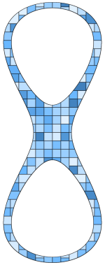
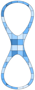
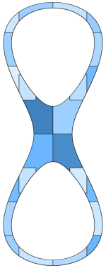
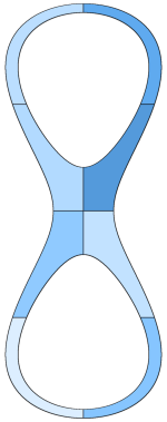
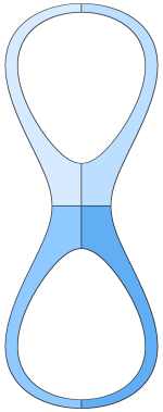
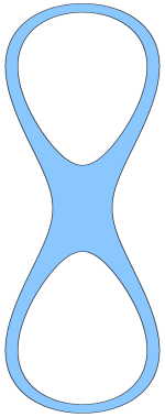
Fine mesh					Bottom level

Figure 8: A single-phase test case applied to a curved domain using implicitly defined meshes. Depicted is the implied $h$-multigrid hierarchy (elements are randomly colored). The coarse meshes are not explicitly constructed in our operator coarsening approach; instead, the discrete gradient and penalty operators and mass matrices are constructed top-down at each level (see Algorithm 1). In particular, note that the bottom level of the hierarchy consists of a mesh with a single element containing two holes.

The first example of a single-phase Poisson problem on a curved domain is illustrated in Figure 8 and consists of a figure-eight domain with two holes surrounded by thin segments. It is important to note that the illustrated mesh hierarchy is implicitly formed by our operator coarsening scheme in Algorithm 1 and it is only the finest-level mesh which is built. On coarser levels, the elements are agglomerated according to the coarsening of the background quadtree; in particular, we note that the bottom level consists of a single element containing two holes. Using the operator coarsening strategy, there is no need to compute quadrature rules for the coarse levels of the mesh hierarchy—the quadrature rules from the fine mesh are effectively coarsened automatically. The results for solving the Dirichlet problem (2.1) using flux coarsening and $h$-multigrid on the curved domain of Figure 8 are shown in Figure 10 (left); we observe good multigrid convergence factors of $\rho\approx 0.05$–$0.2$, nearly independent of grid size, for $1\leq p\leq 5$.

Figure 9: A test case involving a multi-phase elliptic interface problem. Depicted is the implied $h$-multigrid hierarchy, wherein the elements are randomly colored a shade of green or blue for phase one or two, respectively. Similar to Figure 8, only the finest mesh is explicitly constructed; on coarser levels, the discrete gradient and penalty operators and mass matrices are constructed top-down at each level (see Algorithm 1). Note that the bottom level of the hierarchy consists of a mesh of just two elements—the blue element has one component with five holes, whereas the green element consists of six connected components. See the discussion following (4.2) for a description of the noted features A, B, C, D₁, and D₂.

The second example considers a two-phase elliptic interface problem in a rectangular domain illustrated in Figure 9. The corresponding PDE consists of solving

(4.2) $$-\nabla\cdot(\mu_{i}\nabla u) =f \text{in }\Omega_{i}, [\![u]\!] =g_{\Gamma} \text{on }\Gamma,$$

$$u =g_{\partial} \text{on }\partial\Omega, [\![\mu\nabla u\cdot\bm{n}]\!] =h_{\Gamma} \text{on }\Gamma,$$

where $\Gamma$ is the interface between phases $\Omega_{1}$ (green region, with ellipticity coefficient $\mu_{1}=1$) and $\Omega_{2}$ (blue region, with $\mu_{2}=4$), and $[\![\cdot]\!]$ denotes the interfacial jump in the indicated quantity. In this test case, the geometry of the interface has been designed to be challenging—the crescent shape is long and thin; there are three isolated, small circles; and the star shape has sharp cusp-like corners. Once more we note that the illustrated hierarchy in Figure 9 is implicitly formed by the operator coarsening strategy, and only the finest-level mesh is actually built. However, we note that the agglomeration strategy for this multi-phase problem is slightly different from the previous test examples—here, elements are only agglomerated with elements belonging to the same phase. Thus, the interface remains sharp throughout all levels of the hierarchy, and this can dramatically improve the performance of multigrid methods for elliptic interface problems, especially when using high-order accurate techniques [36]. Owing to this agglomeration strategy, coarse mesh levels can have intricate element shapes. Some example features are noted in Figure 9—A indicates a tiny green-phase element surrounded by a large blue-phase element; B indicates two sliver elements; C indicates an element whose cusp-like corners would make it rather difficult to apply a black-box quadrature scheme if one were to explicitly build the coarse-level mesh; and D_1,2 show two green-phase elements, each with multiple connected components (three for D₁ and four for D₂), which is perhaps rather unusual for a finite element method. Another aspect which motivated the present work on operator coarsening is that it would be nearly impossible to directly apply the cell merging algorithms underlying implicitly defined meshes [36] to these coarse levels. Although elements with extreme shapes like these (especially tiny elements next to large elements) can traditionally be of concern for numerical discretization of PDEs, according to our tests they pose no problem when present in the coarse levels of a multigrid solver. Results for solving the homogeneous version of (4.2) ($f$, $g_{\partial}$, $g_{\Gamma}$, and $h_{\Gamma}$ all zero) with a random nonzero initial guess using flux operator coarsening are shown in Figure 10 (right). In this case of an implicitly defined mesh for which different cell merging decisions take place depending on the refinement of the background grid, leading to different mesh topologies as $n$ is increased, we naturally expect some amount of noise in $\rho$. For the majority of grid sizes, we see that the convergence factor $\rho$ is relatively constant, taking values $\rho\approx 0.15$–$0.3$ reflective of the challenging interface geometry; meanwhile, for the largest mesh corresponding to $n=1024$, the slight increase in the convergence rate $\rho$ for all $p$ is attributed to the increased ill-conditioning of the system.

Figure 10: $h$-multigrid convergence factors for flux coarsening and MGPCG applied to the LDG discretization of (left) the single-phase Poisson problem on the curved domain shown in Figure 8 and (right) the multi-phase elliptic interface test problem in (4.2) on the domain shown in Figure 9. The grid size $n$ is the number of cells of the background Cartesian grid required to cover the longest extent of the domain. The plot markers indicate different polynomial orders: $\blacksquare$  , $\bullet$  , $\blacktriangle$  , $\bm{\times}$  , and $\blacksquare$  denote $p=1$, $2$, $3$, $4$, and $5$, respectively.

5 Concluding remarks

We have presented an $hp$-multigrid method for LDG discretizations of elliptic problems that is based on coarsening the discrete gradient and divergence operators from the flux formulation. We have shown that coarsening fine-grid operators in this way results in a method that is equivalent to pure geometric multigrid, but avoids the need to compute quantities associated with coarse meshes, such as lifting operators and quadrature rules. Whereas traditional Galerkin operator coarsening applied to the primal formulation exhibits poor multigrid performance, operator coarsening applied to the flux formulation performs well—convergence factors are nearly independent of both mesh size $h$ and polynomial order $p$ for the demonstrated test problems on uniform Cartesian grids, adaptively refined meshes, and implicitly defined meshes on complex geometries.

Though most of our analysis has focused on the LDG method, we believe that the essential observation applies to other forms of DG discretization of elliptic problems, particularly those in which lifting operators enter the numerical flux for $\bm{q}$. A more thorough analysis for other DG methods and more general choices of numerical fluxes would be required to determine whether the multigrid method described here extends to other methods, such as CDG or HDG. Similarly, though we have employed equal-order elements in this work, i.e., polynomials of the same degree for both $u$ and $\bm{q}$, operator-coarsening for mixed-order elements [13] would be an interesting topic for future investigation.

We considered in this work structured meshes (Cartesian, quadtree, and octree meshes) as well as semi-unstructured, nonconforming, implicitly defined meshes that result from cell merging procedures (see Figures 8 and 9). Applying the multigrid ideas presented here to problems involving more general unstructured meshes is currently under investigation. In this setting, it may be worthwhile to consider different types of relaxation methods owing to their critical role in the overall efficacy of a multigrid method. For example, additive Schwarz smoothers have been shown effective on non-nested polygonal meshes resulting from agglomeration procedures [5]; these smoothers could be studied in the flux coarsening context as well.

The idea of coarsening the divergence and gradient operators separately may also be useful for AMG methods, which currently treat the discrete Laplacian operator in its entirety as a black box. Indeed, black-box AMG algorithms applied to LDG discretizations appear to struggle [30]; perhaps applying AMG separately to the divergence and gradient operators in the flux formulation may yield better results.

References

- [1] P. Antonietti, B. Ayuso de Dios, S. Brenner, and L.-y. Sung, Schwarz methods for a preconditioned WOPSIP method for elliptic problems, Comput. Methods Appl. Math., 12 (2012), pp. 241–272, https://doi.org/doi:10.2478/cmam-2012-0021.
- [2] P. Antonietti, M. Sarti, and M. Verani, Multigrid algorithms for -discontinuous Galerkin discretizations of elliptic problems, SIAM J. Numer. Anal., 53 (2015), pp. 598–618, https://doi.org/10.1137/130947015.
- [3] P. F. Antonietti, P. Houston, X. Hu, M. Sarti, and M. Verani, Multigrid algorithms for -version interior penalty discontinuous Galerkin methods on polygonal and polyhedral meshes, Calcolo, 54 (2017), pp. 1169–1198, https://doi.org/10.1007/s10092-017-0223-6.
- [4] P. F. Antonietti, P. Houston, and G. Pennesi, Fast numerical integration on polytopic meshes with applications to discontinuous Galerkin finite element methods, J. Sci. Comput., 77 (2018), pp. 1339–1370, https://doi.org/10.1007/s10915-018-0802-y.
- [5] P. F. Antonietti and G. Pennesi, V-cycle multigrid algorithms for discontinuous Galerkin methods on non-nested polytopic meshes, J. Sci. Comput., 78 (2019), pp. 625–652, https://doi.org/10.1007/s10915-018-0783-x.
- [6] D. N. Arnold, An interior penalty finite element method with discontinuous elements, SIAM J. Numer. Anal., 19 (1982), pp. 742–760, https://doi.org/10.1137/0719052.
- [7] D. N. Arnold, F. Brezzi, B. Cockburn, and L. D. Marini, Unified analysis of discontinuous Galerkin methods for elliptic problems, SIAM J. Numer. Anal., 39 (2002), pp. 1749–1779, https://doi.org/10.1137/S0036142901384162.
- [8] F. Bassi, A. Ghidoni, S. Rebay, and P. Tesini, High-order accurate -multigrid discontinuous Galerkin solution of the Euler equations, Int. J. Numer. Methods Fluids, 60 (2008), pp. 847–865, https://doi.org/10.1002/fld.1917.
- [9] F. Bassi and S. Rebay, A high-order accurate discontinuous finite element method for the numerical solution of the compressible Navier–Stokes equations, J. Comput. Phys., 131 (1997), pp. 267–279, https://doi.org/10.1006/jcph.1996.5572.
- [10] F. Bassi, S. Rebay, G. Mariotti, S. Pedinotti, and M. Savini, A high-order accurate discontinuous finite element method for inviscid and viscous turbomachinery flows, in Proceedings of the 2nd European Conference on Turbomachinery Fluid Dynamics and Thermodynamics, Technologisch Instituut, Antwerpen, Belgium, 1997, pp. 99–109.
- [11] P. Bastian, M. Blatt, and R. Scheichl, Algebraic multigrid for discontinuous Galerkin discretizations of heterogeneous elliptic problems, Numer. Lin. Alg. Appl., 19 (2012), pp. 367–388, https://doi.org/10.1002/nla.1816.
- [12] S. C. Brenner and J. Zhao, Convergence of multigrid algorithms for interior penalty methods, Appl. Numer. Anal. & Comput. Math., 2 (2005), pp. 3–18, https://doi.org/10.1002/anac.200410019.
- [13] F. Brezzi, T. J. R. Hughes, L. D. Marini, and A. Masud, Mixed discontinuous Galerkin methods for darcy flow, J. Sci. Comput., 22 (2005), pp. 119–145, https://doi.org/10.1007/s10915-004-4150-8.
- [14] F. Brezzi, G. Manzini, D. Marini, P. Pietra, and A. Russo, Discontinuous Galerkin approximations for elliptic problems, Numerical Methods for Partial Differential Equations, 16 (2000), pp. 365–378, https://doi.org/10.1002/1098-2426(200007)16:4<365::AID-NUM2>3.0.CO;2-Y.
- [15] W. L. Briggs, V. E. Henson, and S. F. McCormick, A Multigrid Tutorial, Second Edition, Society for Industrial and Applied Mathematics, 2000, https://doi.org/10.1137/1.9780898719505.
- [16] P. Castillo, B. Cockburn, I. Perugia, and D. Schötzau, An a priori error analysis of the local discontinuous Galerkin method for elliptic problems, SIAM J. Numer. Anal., 38 (2000), pp. 1676–1706, https://doi.org/10.1137/S0036142900371003.
- [17] B. Cockburn and B. Dong, An analysis of the minimal dissipation local discontinuous Galerkin method for convection–diffusion problems, J. Sci. Comput., 32 (2007), pp. 233–262, https://doi.org/10.1007/s10915-007-9130-3.
- [18] B. Cockburn, J. Gopalakrishnan, and R. Lazarov, Unified hybridization of discontinuous Galerkin, mixed, and continuous Galerkin methods for second order elliptic problems, SIAM J. Numer. Anal., 47 (2009), pp. 1319–1365, https://doi.org/10.1137/070706616.
- [19] B. Cockburn, G. Kanschat, I. Perugia, and D. Schötzau, Superconvergence of the local discontinuous Galerkin method for elliptic problems on Cartesian grids, SIAM J. Numer. Anal., 39 (2001), pp. 264–285, https://doi.org/10.1137/S0036142900371544.
- [20] B. Cockburn and C.-W. Shu, The local discontinuous Galerkin method for time-dependent convection-diffusion systems, SIAM J. Numer. Anal., 35 (1998), pp. 2440–2463, https://doi.org/10.1137/S0036142997316712.
- [21] J. Douglas and T. Dupont, Interior penalty procedures for elliptic and parabolic Galerkin methods, in Computing Methods in Applied Sciences, R. Glowinski and J. L. Lions, eds., Berlin, Heidelberg, 1976, Springer, pp. 207–216, https://doi.org/10.1007/BFb0120591.
- [22] M. S. Fabien, M. G. Knepley, R. T. Mills, and B. M. Riviere, Heterogeneous computing for a hybridizable discontinuous Galerkin geometric multigrid method, May 2017, https://arxiv.org/abs/1705.09907.
- [23] K. J. Fidkowski, T. A. Oliver, J. Lu, and D. L. Darmofal, -multigrid solution of high-order discontinuous Galerkin discretizations of the compressible Navier–Stokes equations, J. Comput. Phys., 207 (2005), pp. 92–113, https://doi.org/10.1016/j.jcp.2005.01.005.
- [24] J. Gopalakrishnan and G. Kanschat, A multilevel discontinuous Galerkin method, Numer. Math., 95 (2003), pp. 527–550, https://doi.org/10.1007/s002110200392.
- [25] B. T. Helenbrook, D. Mavriplis, and H. L. Atkins, Analysis of -multigrid for continuous and discontinuous finite element discretizations, in 16th AIAA Computational Fluid Dynamics Conference, 2003, https://doi.org/10.2514/6.2003-3989.
- [26] J. S. Hesthaven and T. Warburton, Nodal Discontinuous Galerkin Methods: Algorithms, Analysis, and Applications, vol. 54 of Texts in Applied Mathematics, Springer, New York, 2008, https://doi.org/10.1007/978-0-387-72067-8.
- [27] G. Kanschat, Preconditioning methods for local discontinuous Galerkin discretizations, SIAM J. Sci. Comput., 25 (2003), pp. 815–831, https://doi.org/10.1137/S1064827502410657.
- [28] G. Kanschat, Multilevel methods for discontinuous Galerkin FEM on locally refined meshes, Computers & Structures, 82 (2004), pp. 2437–2445, https://doi.org/10.1016/j.compstruc.2004.04.015.
- [29] H. Luo, J. D. Baum, and R. Löhner, A -multigrid discontinuous Galerkin method for the Euler equations on unstructured grids, J. Comput. Phys., 211 (2006), pp. 767–783, https://doi.org/10.1016/j.jcp.2005.06.019.
- [30] L. N. Olson and J. B. Schroder, Smoothed aggregation multigrid solvers for high-order discontinuous Galerkin methods for elliptic problems, J. Comput. Phys., 230 (2011), pp. 6959–6976, https://doi.org/10.1016/j.jcp.2011.05.009.
- [31] J. Peraire and P.-O. Persson, The compact discontinuous Galerkin (CDG) method for elliptic problems, SIAM J. Sci. Comput., 30 (2008), pp. 1806–1824, https://doi.org/10.1137/070685518.
- [32] P.-O. Persson, A sparse and high-order accurate line-based discontinuous Galerkin method for unstructured meshes, Journal of Computational Physics, 233 (2013), pp. 414–429, https://doi.org/10.1016/j.jcp.2012.09.008.
- [33] I. Perugia and D. Schötzau, An -analysis of the local discontinuous Galerkin method for diffusion problems, J. Sci. Comput., 17 (2002), pp. 561–571, https://doi.org/10.1023/A:1015118613130.
- [34] F. Prill, M. Lukáčová-Medviďová, and R. Hartmann, Smoothed aggregation multigrid for the discontinuous Galerkin method, SIAM J. Sci. Comput., 31 (2009), pp. 3503–3528, https://doi.org/10.1137/080728457.
- [35] R. I. Saye, High-order quadrature methods for implicitly defined surfaces and volumes in hyperrectangles, SIAM J. Sci. Comput., 37 (2015), pp. A993–A1019, https://doi.org/10.1137/140966290.
- [36] R. I. Saye, Implicit mesh discontinuous Galerkin methods and interfacial gauge methods for high-order accurate interface dynamics, with applications to surface tension dynamics, rigid body fluid–structure interaction, and free surface flow: Part I, J. Comput. Phys., 344 (2017), pp. 647–682, https://doi.org/10.1016/j.jcp.2017.04.076.
- [37] R. I. Saye, Implicit mesh discontinuous Galerkin methods and interfacial gauge methods for high-order accurate interface dynamics, with applications to surface tension dynamics, rigid body fluid–structure interaction, and free surface flow: Part II, J. Comput. Phys., 344 (2017), pp. 683–723, https://doi.org/10.1016/j.jcp.2017.05.003.
- [38] C. Siefert, R. Tuminaro, A. Gerstenberger, G. Scovazzi, and S. S. Collis, Algebraic multigrid techniques for discontinuous Galerkin methods with varying polynomial order, Computational Geosciences, 18 (2014), pp. 597–612, https://doi.org/10.1007/s10596-014-9419-x.
- [39] J. Stiller, Robust multigrid for high-order discontinuous Galerkin methods: A fast Poisson solver suitable for high-aspect ratio Cartesian grids, J. Comput. Phys., 327 (2016), pp. 317–336, https://doi.org/10.1016/j.jcp.2016.09.041.
- [40] M. Sussman, A. S. Almgren, J. B. Bell, P. Colella, L. H. Howell, and M. L. Welcome, An adaptive level set approach for incompressible two-phase flows, J. Comput. Phys., 148 (1999), pp. 81–124, https://doi.org/10.1006/jcph.1998.6106.
- [41] O. Tatebe, The multigrid preconditioned conjugate gradient method, in The Sixth Copper Mountain Conference on Multigrid Methods, NASA Langley Research Center, 1993, pp. 621–634.
- [42] J. Xu, Iterative methods by space decomposition and subspace correction, SIAM Review, 34 (1992), pp. 581–613, https://doi.org/10.1137/1034116.
- [43] J. Yan and C.-W. Shu, Local discontinuous Galerkin methods for partial differential equations with higher order derivatives, J. Sci. Comput., 17 (2002), pp. 27–47, https://doi.org/10.1023/A:1015132126817.