Tensor models for linguistics pitch curve data of native speakers of Afrikaans

Abstract

We use tensor analysis techniques for high-dimensional data to gain insight into pitch curves, which play an important role in linguistics research. In particular, we propose that demeaned phonetics pitch curve data can be modeled as having a Kronecker product inverse covariance structure with sparse factors corresponding to words and time. Using data from a study of native Afrikaans speakers, we show that by targeting conditional independence through a graphical model, we reveal relationships associated with natural properties of words as studied by linguists. We find that words with long vowels cluster based on whether the vowel is pronounced at the front or back of the mouth, and words with short vowels have strong edges associated with the initial consonant.

1 Introduction

Pitch curve data in phonetics is used to address a wide variety of research questions, including studying the cognitive processes of sound perception and production (Chetouani et al., 2009; Shami and Verhelst, 2007; Sheikhan et al., 2013), population variation in speech patterns, and software generation of speech (Hirst, 2011; Houde and Jordan, 1998; Iriondo et al., 2009). To obtain pitch curve data, human speech is recorded, and pitch (in Hz) is extracted at a dense sequence of time points. Linguists are interested in the relationship between pitch and other attributes of spoken words, which gives insight into how meaning is conveyed through acoustical properties of speech. Extensive research has documented associations between pitch curves and acoustical characteristics of words such as voicing (Hanson, 2009). Such pitch curve analysis has traditionally employed parametric models such as mixed effects models with random effects for speaker and word (Baayen et al., 2008). By contrast, we use a more flexible matrix-variate model that focuses on word-word and time-time covariances. By analyzing data from Coetzee et al. (2018), we show that word-word correlations are associated with word attributes of interest to linguists.

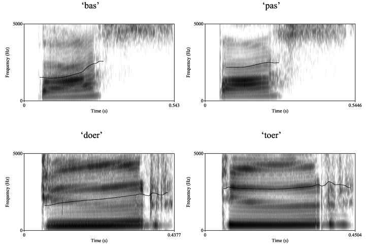
(a) Spectrograms from Coetzee et. al. 2017.

(b) Vowel formant diagram from Wissing (2012).

Figure 1: Phonetics data in Afrikaans.

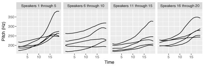
(a) Pitch curves for the word ``met.'' For readability, the pitch curves are displayed in four panels.

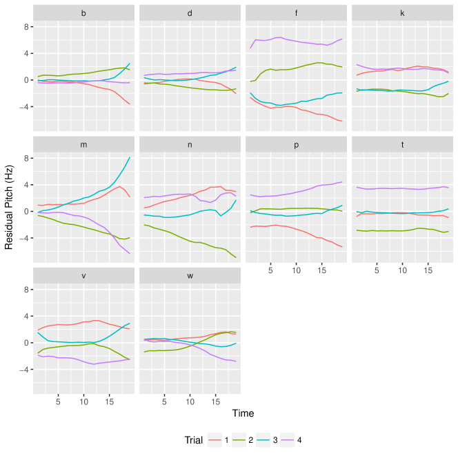
(b) Trial residualized pitch curves for each of the four trials, averaged over speaker and word for each initial consonant.

Figure 2: Phonetics pitch curve data in Afrikaans.

Here we propose a Kronecker product model and de-meaning procedure for pitch curve data, yielding correlation and precision information along two axes–words and time points. Using estimated precision matrices and associated graphical models, we show that word-word correlations are driven by natural properties of words studied in phonetics, including onset (initial consonant), coda (final consonant), and mouth position. In particular, we find words with long vowels naturally cluster according to the region of the mouth in which the vowel is pronounced (front of mouth vs. back of mouth). We furthermore show that time-time covariance matrices are similar across subsets of words, which justifies pooling words to estimate a common time-time covariance matrix.

To estimate covariance matrices, inverse covariance matrices, and graphical models, we use statistical methods with rigorous theoretical guarantees (Zhou, 2014). In particular, we use Gemini and nodewise regression with theoretically guided penalty parameters. The data contains trial replicates, with four utterances of each word by each speaker; we make use of trial residualization to center the data prior to estimating the covariance matrices. Due to stable inter-individual differences in speech patterns, unadjusted covariance matrices are highly ill-conditioned. We therefore developed a non-parametric demeaning procedure such that the residuals were suitable for graphical analysis. We anticipate that this approach will be useful in other types of data with trial replicates, including linguistics and neuroscience data.

Figure 1(a) displays the spectrogram of four words in Afrikaans, in which the darkness represents amplitude as a function of frequency and time. To provide a basic illustration of pitch curve data, in Figure 2(a) we display the first utterance of the word ``met'' for each of the speakers. For ease of visualization, the pitch curves for the speakers are displayed in four panels. These are individual raw pitch curves that have not been centered or averaged. The pitch curves are obtained by segmenting the word to extract the vowel, then extracting pitch measurements at $19$ equally spaced time points within the vowel, using Praat  (Boersma, 1993). There is substantial heterogeneity among speakers pronouncing a given word. As discussed below, we center the data using trial residualization, subtracting from each individual pitch curve the corresponding point-wise mean pitch curve over each subject $\times$ word, taken over the four trials. To illustrate, in Figure 2(b), we display four trials, centered by first removing the speaker $\times$ word mean, and then averaging these residuals over speakers and words within initial consonant (with a separate panel shown for each initial consonant). The trials are centered as discussed below in equation (2).

The raw data we consider here (Coetzee et al., 2018) can be represented as a four-index array. Specifically, let $X(i,j,r,t)$ denote the pitch measurement for speaker $i$, word $j$, trial $r$, and time $t$. Let $n(s)$, $n(w)$, $n(r)$, and $n(t)$ denote the respective dimension along each axis. We describe a matrix-variate model that captures word-word and time-time correlations, treating the trials as replicates nested within speakers by words. Let $X(i,r)\in\mathbb{R}^{n(w)\times n(t)}$ denote the data for speaker $i$, trial $r$. For the mean structure, we assume that for each speaker $i$, a common mean matrix $M(i)\in\mathbb{R}^{n(w)\times n(t)}$ is shared across the four trials. Denote the sample mean estimate of $M(i)$ as

$$\overline{X}(i)=\frac{1}{n(r)}\sum_{r=1}^{n(r)}X(i,r),$$ (1)

with $M(i)=\mathbb{E}\left[\overline{X}(i)\right]$. For the covariance structure, we specify a Kronecker product model. Hence the mean and covariance structure can be expressed, respectively, as

$$\mathbb{E}\left[X(i,r)-\overline{X}(i)\right]=0\qquad\text{ and }\qquad\text{Cov}(\text{vec}(X(i,r)))=A\otimes B,$$ (2)

where $A$ is a time-time covariance matrix and $B$ is a word-word covariance matrix.

We use estimation procedures with known convergence properties to recover $A$ and $B$ from the data, then use the corresponding estimated graph structures to probe word-word and time-time associations.

The following definitions, taken verbatim from Zhou (2014), concerns Gaussian graphical models for random vectors and matrices, respectively.

Definition 1.1.

Let $V=(V_{1},\ldots,V_{n})^{T}$ be a random Gaussian vector, which we represent by an undirected graph $G=(\mathcal{V},F)$. The vertex set $\mathcal{V}:=\{1,\ldots,n\}$ has one vertex for each component of the vector $V$. The edge set $F$ consists of pairs $(j,k)$ that are joined by an edge. If $V_{j}$ is independent of $V_{k}$ given the other variables, then $(j,k)\notin F$.

Definition 1.2.

Let $\mathcal{V}=\{1,\ldots,n\}$ be an index set which enumerates rows of $X$ according to a fixed order. For all $i=1,\ldots,m$, we assign to each variable of a column vector $x^{i}$ exactly one element of the set $\mathcal{V}$ by a rule of correspondence $g:x^{i}\to\mathcal{V}$ such that $g(x^{i}_{j})=j,j=1,\ldots,n$. The graphs $G_{i}(\mathcal{V},F)$ constructed for each random column vector $x^{i},i=1,\ldots,m$ according to Definition 1.1 will share an identical edge set $F$, because the normalized column vectors ${x^{1}}/{\sqrt{a_{11}}},\ldots,x^{m}/\sqrt{a_{mm}}$ follow the same multivariate normal distribution ${\mathcal{N}}_{n}(0,B)$, where $a_{jj}$ denotes the $j$th diagonal entry of $A$ as defined in (2). Hence, graphs $G_{1},\ldots,G_{m}$ are isomorphic and we write $G_{i}\simeq G_{j},\forall i,j$. Due to the isomorphism, we use $G(\mathcal{V},F)$ to represent the family of graphs $G_{1},\ldots,G_{m}$. Hence, a pair $(\ell,k)$ which is absent in $F$ encodes conditional independence between the ${\ell}$th row and the $k$th row given all other rows. Similarly, let $\Gamma=\{1,\ldots,m\}$ be the index set which enumerates columns of $X$ according to a fixed order. We use $H(\Gamma,E)$ to represent the family of graphs $H_{1},\ldots,H_{f}$, where $H_{i}$ is constructed for row vector $y^{i}$, and $H_{i}\simeq H_{j},\forall i,j$. Now $H(\Gamma,E)$ is a graph with adjacency matrix $\Upsilon(H)=\Upsilon(A^{-1})$ as edges in $E$ encode nonzeros in $A^{-1}$, and $G(\mathcal{V},F)$ is a graph with adjacency matrix $\Upsilon(G)=\Upsilon(B^{-1})$.

The bigraphical lasso (Kalaitzis et al., 2013) models the graph as Cartesian product of $G(\mathcal{V},F)$ and $H(\Gamma,E)$.

2 Methods

We define the sample covariance matrices based on trial residualized data. We then define the Gemini estimators and nodewise regression.

2.1 Covariance and precision matrices for time points and words

In analyzing data from Coetzee et al. (2018), we treat the $20$ subjects and four trials in the Afrikaans study as $20\times 4=80$ independent random arrays with a common covariance structure. Each such array is a $n(w)\times n(t)$ matrix which has been centered over the trials as discussed above in (2). We then apply the Glasso method with theoretically guided penalty parameters to the word and time Gram matrices. This approach gives us graph structures among the words and among the time points.

We now define the sample covariance matrices based on trial residualization; the corresponding sample correlation matrices are used as inputs to Gemini and nodewise regression. Let $S_{A}$ denote the word-word sample covariance matrix,

$$S_{A}=\frac{1}{n(t)n(s)n(r)}\sum_{i=1}^{n(s)}\sum_{r=1}^{n(r)}\left[X(i,r)-\overline{X}(i)\right]\left[X(i,r)-\overline{X}(i)\right]^{T}$$ (3)

and let $S_{B}$ denote the time-time sample covariance matrix,

$$S_{B}=\frac{1}{n(w)n(s)n(r)}\sum_{i=1}^{n(s)}\sum_{r=1}^{n(r)}\left[X(i,r)-\overline{X}(i)\right]^{T}\left[X(i,r)-\overline{X}(i)\right].$$ (4)

Note that in this formulation, speakers and trials are taken as replicates, so each Gram matrix is an average of $n(s)\cdot n(r)$ Gram matrices.

Gemini estimators. Let the sample correlation matrices corresponding to (3) and (4) be defined as

$$\widehat{\Gamma}_{ij}(A)=\frac{(S_{A})_{ij}}{\sqrt{(S_{A})_{ii}(S_{A})_{jj}}}\quad\text{ and }\quad\widehat{\Gamma}_{ij}(B)=\frac{(S_{B})_{ij}}{\sqrt{(S_{B})_{ii}(S_{B})_{jj}}}.$$ (5)

The Gemini estimators apply graphical lasso with adjusted penalty to account for correlation along the other axis. The Gemini inverse correlation estimators  (Zhou, 2014) are defined as follows, using a pair of penalized estimators for the correlation matrices $\rho(A)=(a_{ij}/\sqrt{a_{ii}a_{jj}})$ and $\rho(B)=(b_{ij}/\sqrt{b_{ii}b_{jj}})$,

$$\widehat{A}_{\rho} =\mathop{\text{arg\,min}\kern 0.86108pt}_{A_{\rho}\succ 0}\left\{\operatorname{tr}\left(\widehat{\Gamma}(A)A_{\rho}^{-1}\right)+\log|A_{\rho}|+\lambda_{B}|A_{\rho}^{-1}|_{1,\text{off}}\right\}\quad\text{ and }$$ (6)

$$\widehat{B}_{\rho} =\mathop{\text{arg\,min}\kern 0.86108pt}_{B_{\rho}\succ 0}\left\{\operatorname{tr}\left(\widehat{\Gamma}(B)B_{\rho}^{-1}\right)+\log|B_{\rho}|+\lambda_{A}|B_{\rho}^{-1}|_{1,\text{off}}\right\},$$ (7)

where the inputs are a pair of sample correlation matrices as defined in (5). The theoretically guided penalty parameters used in (6) and (7) are

$$\lambda_{A}=\sqrt{\frac{\log(n(w))}{n(s)\cdot n(r)\cdot n(w)}}\qquad\text{and}\qquad\lambda_{B}=\sqrt{\frac{\log(n(w))}{n(s)\cdot n(r)\cdot n_{\text{eff}}(t)}},$$ (8)

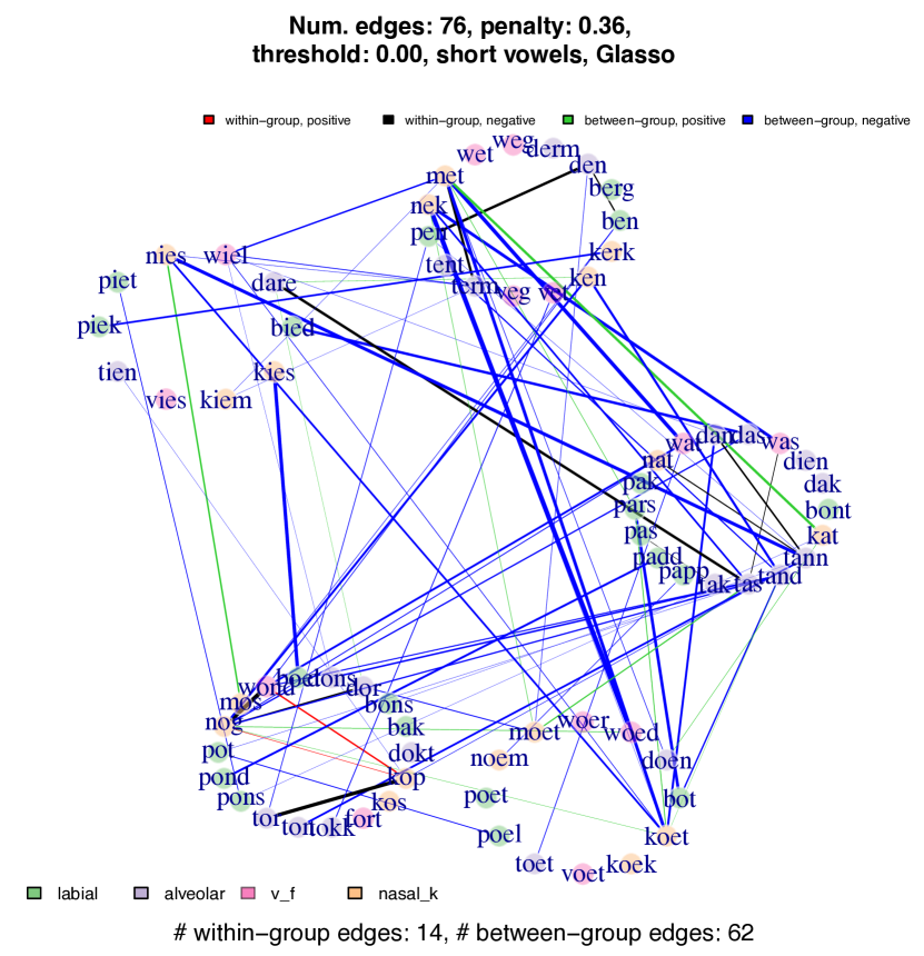
Figure 27: Inverse covariance graph of words with short vowels, estimated using Glasso regression, organized by vowel.

where $n(w)$ is the number of words, $n(s)$ is the number of speakers, $n(r)$ is the number of replicates, and $n_{\text{eff}}(t)$ is the number of ``effective'' time points. Note that the effective time points per utterance is smaller than $19$, because the pitch curves are smooth curves, so adjacent points are dependent. Due to the stretched time scale over short vowels versus the long vowels, we believe that $n_{\text{eff}}(t)$ for short vowels is smaller than that for long ones; hence we recommend using larger penalty when we interpret the graphs over short vowels. Figures 27 through 30 in the Appendix illustrate that edges persist at higher penalty values for words with short vowels than for words with long vowels.

2.2 Nodewise regression

In addition to using Glasso, we also estimate edges using nodewise regression. Meinshausen and Bühlmann (2006) proposed variable selection via nodewise regression, in which each variable is regressed on each other variable via $\ell_{1}$ penalized regression. The edges correspond to the nonzero entries of the regression coefficients (i.e. an edge exists between vertices $i$ and $j$ if either the regression coefficient of variable $i$ on $j$ is nonzero, or the regression coefficient of variable $j$ on $i$ is nonzero). Meinshausen and Bühlmann (2006) proved variable selection consistency of nodewise regression.

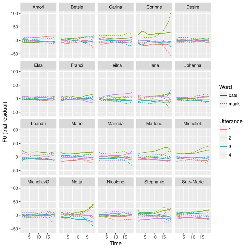
Figure 15: Trial residual pitch curves for the words bate and maak.

We define Pearson correlation. For random variables $X,Y\in\mathbb{R}$, the population Pearson correlation is defined as $\rho(X,Y)=\text{Cov}(X,Y)/\sqrt{\text{Var}(X)\text{Var}(Y)}$. For example, the Pearson correlation between ``bate'' and ``maak'' is $0.50$, with trial residualized pitch curves displayed in Figure 15 in the appendix. Let $\widehat{\Gamma}$ denote a sample Pearson correlation matrix as defined in (5).

We now explain nodewise regression in more detail. Let $\widehat{\Gamma}^{(i)}\in\mathbb{R}^{(m-1)\times(m-1)}$ denote the submatrix of $\widehat{\Gamma}$ obtained by excluding the $i$th column and $i$th row. Let $\widehat{\gamma}^{(i)}$ denote the $i$th column of $\widehat{\Gamma}$ excluding the diagonal entry. The regression coefficient for the $i$th variable is obtained by solving the $\ell_{1}$ penalized least squares problem,

$$\widehat{\beta}^{i}=\text{arg min}_{\beta:\beta\in\mathbb{R}^{m-1}}\left\{\frac{1}{2}\beta^{T}\widehat{\Gamma}^{(i)}\beta-\langle\widehat{\gamma}^{(i)},\beta\rangle+\lambda\lVert\beta\rVert_{1}\right\}.$$ (9)

Afterwards, the inverse correlation matrix is reconstructed by first obtaining a matrix $\widetilde{\Theta}$,

$$\widetilde{\Theta}_{-j,-j}=-(\widehat{\Gamma}_{jj}-\widehat{\Gamma}_{j,-j}\widehat{\beta}^{j})^{-1}\widehat{\beta}^{j},\quad\text{and}\quad\widetilde{\Theta}_{jj}=(\widehat{\Gamma}_{jj}-\widehat{\Gamma}_{j,-j}\widehat{\beta}^{j})^{-1},$$ (10)

then projecting $\widetilde{\Theta}$ onto the space of symmetric matrices.

Using nodewise regression with a refit to obtain an estimate of the inverse covariance matrix was proposed by Yuan (2010); Loh and Wainwright (2012). In Zhou et al. (2011a), they combine a multiple regression approach with ideas of thresholding and refitting: first they infer a sparse undirected graphical model structure via thresholding of each among many $\ell_{1}$-norm penalized regression functions of (9). They show that under suitable conditions, this approach yields consistent estimation in terms of graphical structure and fast convergence rates with respect to the operator and Frobenius norm for the covariance matrix and its inverse. In our data analysis, using the same penalty parameters for nodewise regression as defined in (8) follows the theoretical guidance of Zhou et al. (2011a) and yields similar edge structures and sparsity levels to Glasso.

Our nodewise regression with thresholding procedure follows from ideas of Zhou et al. (2011a) and Zhou (2010). Since our input matrix is positive semidefinite, the methods of Loh and Wainwright (2012), Yuan (2010), and Zhou et al. (2011b) would all work to obtain $\Theta$.

3 Data Analysis

3.1 Long vowel conditional dependence is driven by front/back of mouth pronunciation

We show that for words with long vowels, a natural clustering exists in the edges of the graphical model according to whether the vowel is pronounced toward the front of the mouth or the back of the mouth. In Figure 1(b), vowels on the left are pronounced in the front of the mouth (i, ), whereas vowels on the right are pronounced in the back of the mouth (, , u). Figure 3 in the Appendix displays the estimated inverse covariance graph for words with long vowels, using Glasso with a penalty of $0.3$. Based on the estimated effective sample size ($n(r)=3$, $n_{\text{eff}}(t)=3$ or $4$, $n(s)=20$) and theoretical guidance from Zhou (2014), we believe the theoretical penalty should be in the range of $[0.11,0.13]$, so a penalty of $0.3$ displays the strongest edges. Based on the edges, the words naturally cluster according to whether the vowels are spoken at the front or back of the mouth. The sum of the absolute values of within-cluster Glasso-estimated edge weights is $0.76$, whereas the sum of between-cluster edge weights is $0.18$ (i.e. the total edge weight of edges that cross the graph cut is substantially larger).

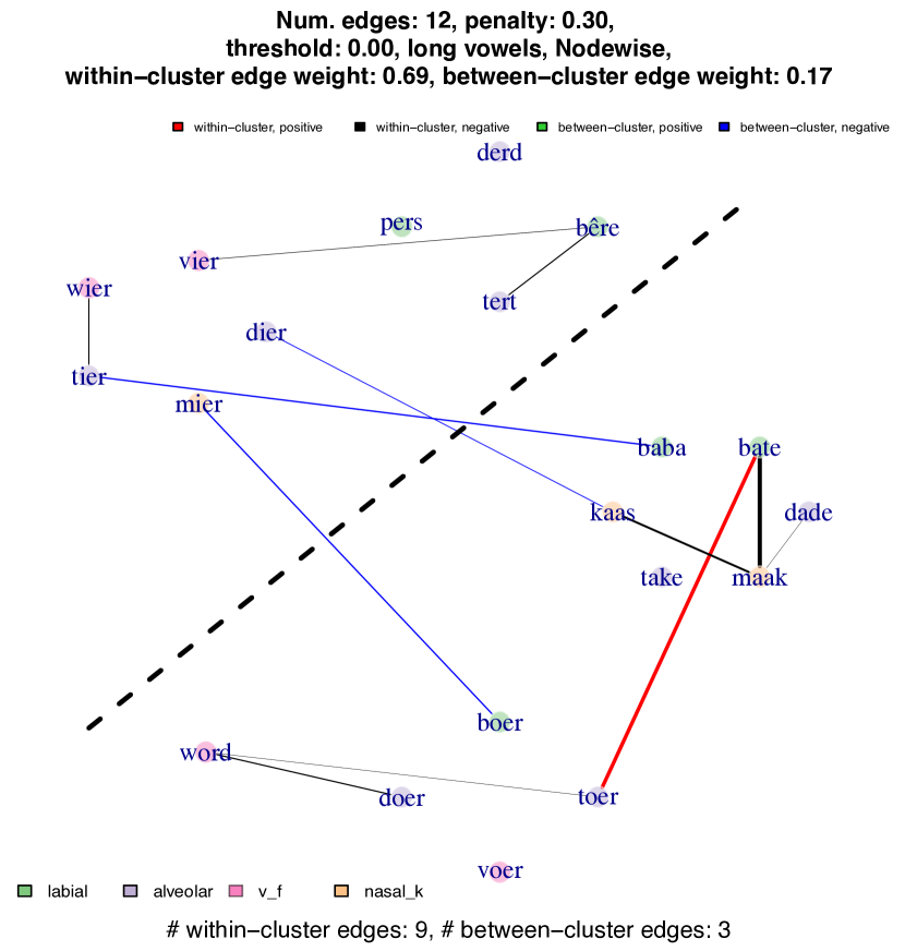
Figure 10: Inverse correlation edge graph for words with long vowels. Based on the estimated effective sample ($n(r)=3$, $n_{\text{eff}}(t)=3$ or $4$, $n(s)=20$) and the theoretical guidance from  Zhou (2014), we believe the theoretical penalty should be in the range of $[0.11,0.13]$. The words are organized by vowel, with each circle of words sharing a common vowel (``word'' is the only word with a long   vowel; in Afrikaans, it means ``become'').

Figure 4 displays a bar chart of the fraction of edges present among each pair of long vowels. The edges are estimated using a sequence of penalty parameters for Glasso and nodewise regression. Note that when the penalty is zero, the Glasso estimate reduces to the inverse sample correlation, which is a fully dense matrix, so the fraction of edges is equal to one. As the penalty increases, the fraction of edges decreases more rapidly for some vowel pairs than for others. For word pairs that have larger Pearson correlation but smaller penalized inverse correlation, the words are marginally correlated, but not conditionally correlated given the other words; that is, the relationship between those words is explained by other words. As seen in Figure 4, the long vowel pairs - and -u, both of which are spoken at the front of the mouth, persist to a penalty of $0.4$. By contrast, the between-cluster edges drop out first as the penalty increases. For example, the /æ-vowel pairs have many edges at smaller penalty parameters, but no edges at a penalty of $0.3$. Figure 10 displays the estimated inverse covariance graph for words with long vowels, using nodewise regression with a penalty of $0.3$.

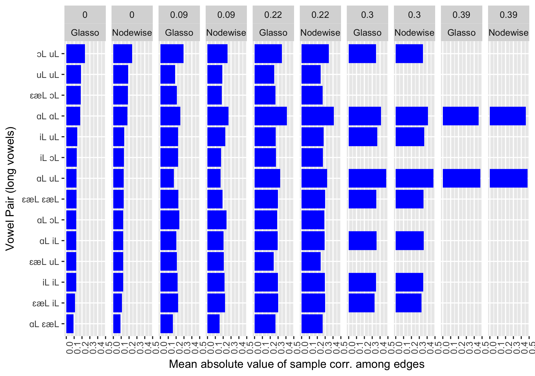
Figure 11: Bar chart of average sample correlation among edges for long vowels, estimated using Glasso and nodewise regression.

For each pair of long vowels, Figure 11 displays the average absolute values of the Pearson correlation entries among edges. Note that the edges are obtained via the precision matrix, but the average is taken using entries of the sample correlation matrix. For example, let $E(A,A)$ denote the set of edges between words with a long ``'' vowel, and let $|E(A,A)|$ denote the number of edges between words with long ``'' vowels. Then we calculate

$$\frac{1}{|E(A,A)|}\sum_{(i,j)\in E(A,A)}|S_{ij}|.$$ (11)

Note that as the penalty increases, the number of edges decreases, so the average Pearson correlation is taken over the stronger edges that remain, resulting in a larger value. At the highest penalty shown, three edges remain: bate-maak, maak-kaas, and bate-toer. Pearson correlations between word pairs with strong edges are shown in Table 2.

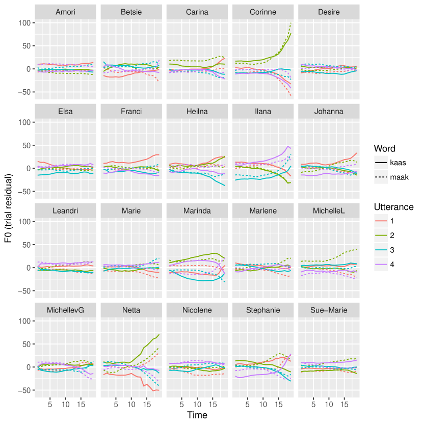
Figure 14: Trial residual pitch curves for the words maak and kaas.

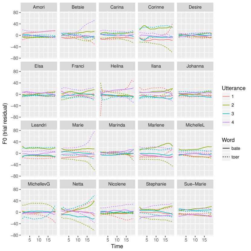
Figure 16: Trial residual pitch curves for the words bate and toer.

Figure 14 displays the trial residual pitch curves for maak and kaas. For multiple speakers, the variability increases towards the end of the word, flaring out over time. The Pearson correlation between two words is high if corresponding utterances within speakers predominantly have the same sign (e.g. if the first utterance of maak is positive for the same time points as the first utterance of kaas, the second utterance of maak is positive for the same time points as the second utterance of kaas, etc., and if this pattern holds across speakers). Analgously, Figure 15 shows the trial residual pitch curves for bate and maak. Figure 16 shows the trial residual pitch curves for bate and toer.

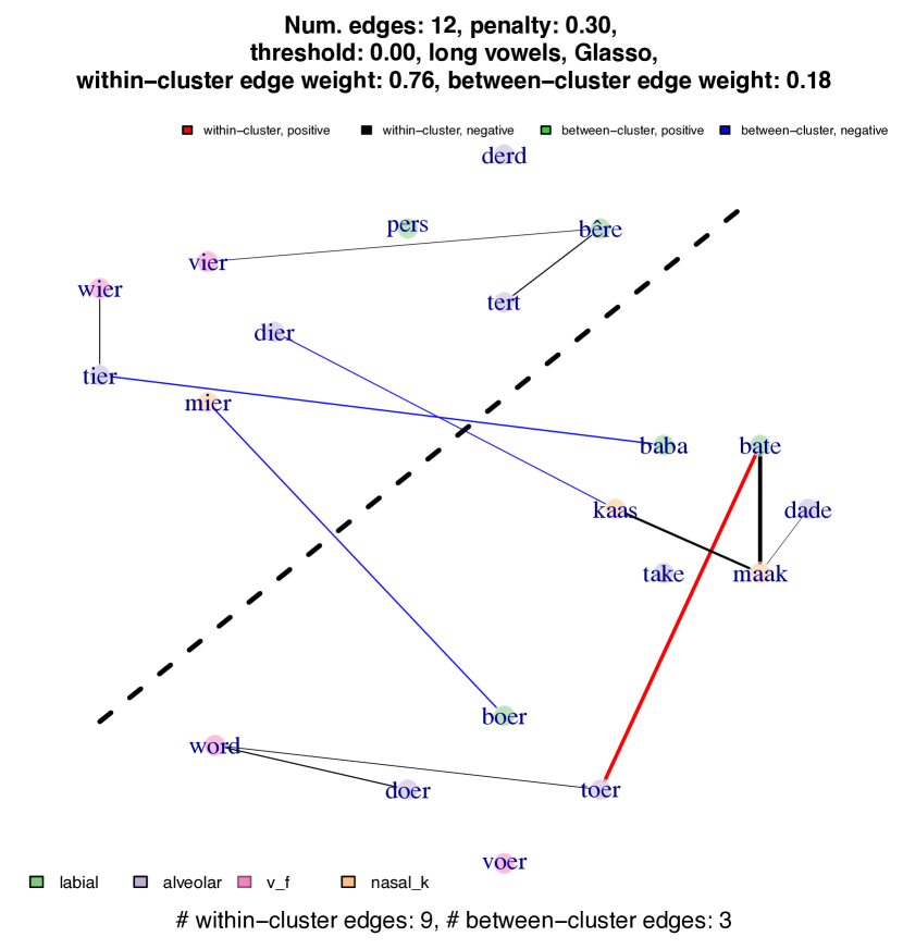
Figure 3: Inverse correlation edge graph for words with long vowels. The words are organized by vowel, with each circle of words sharing a common vowel. The words cluster based on whether the vowel is pronounced in the front of the mouth (upper cluster) or back of the mouth (lower cluster); see Figure 1(b).

Figure 4: Bar chart of fraction of edges for long vowels, estimated using Glasso and nodewise regression.

3.2 Short vowel conditional dependence is associated with initial and final consonants

Among words with short vowels, edges are associated with word attributes including onset (initial consonant) and coda (consonant after the vowel). Among edges that persist to a penalty of $0.52$ are words beginning with n and w (both continuously voiced), m and w (also continuously voiced), and n and t (both alveolar). Figure 5 (and Section B.4 in the appendix) displays bar charts of the average sample correlation corresponding to edges between words with short vowels for each pair of onsets, first codas, and last codas.

(a) Bar chart of average sample correlation between words with edges for each pair of onsets, estimated using Glasso and nodewise regression.

(b) Bar chart of average sample correlation between words with edges for each pair of first codas, estimated using Glasso and nodewise regression.

Figure 5: Bar charts for short vowels.

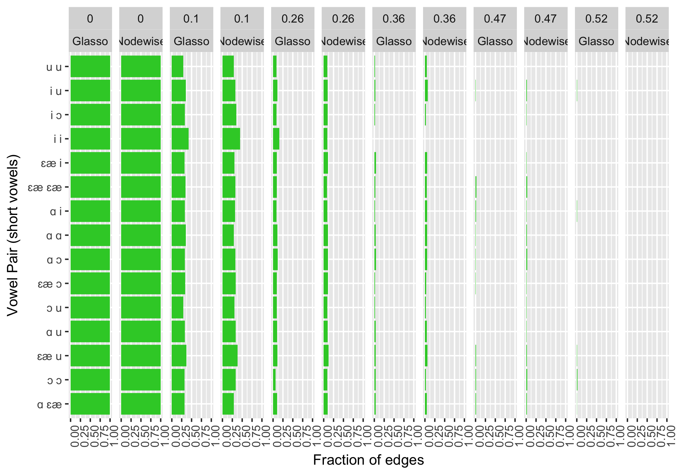
Figure 12: Bar chart of fraction of edges for short vowels, estimated using Glasso and nodewise regression.

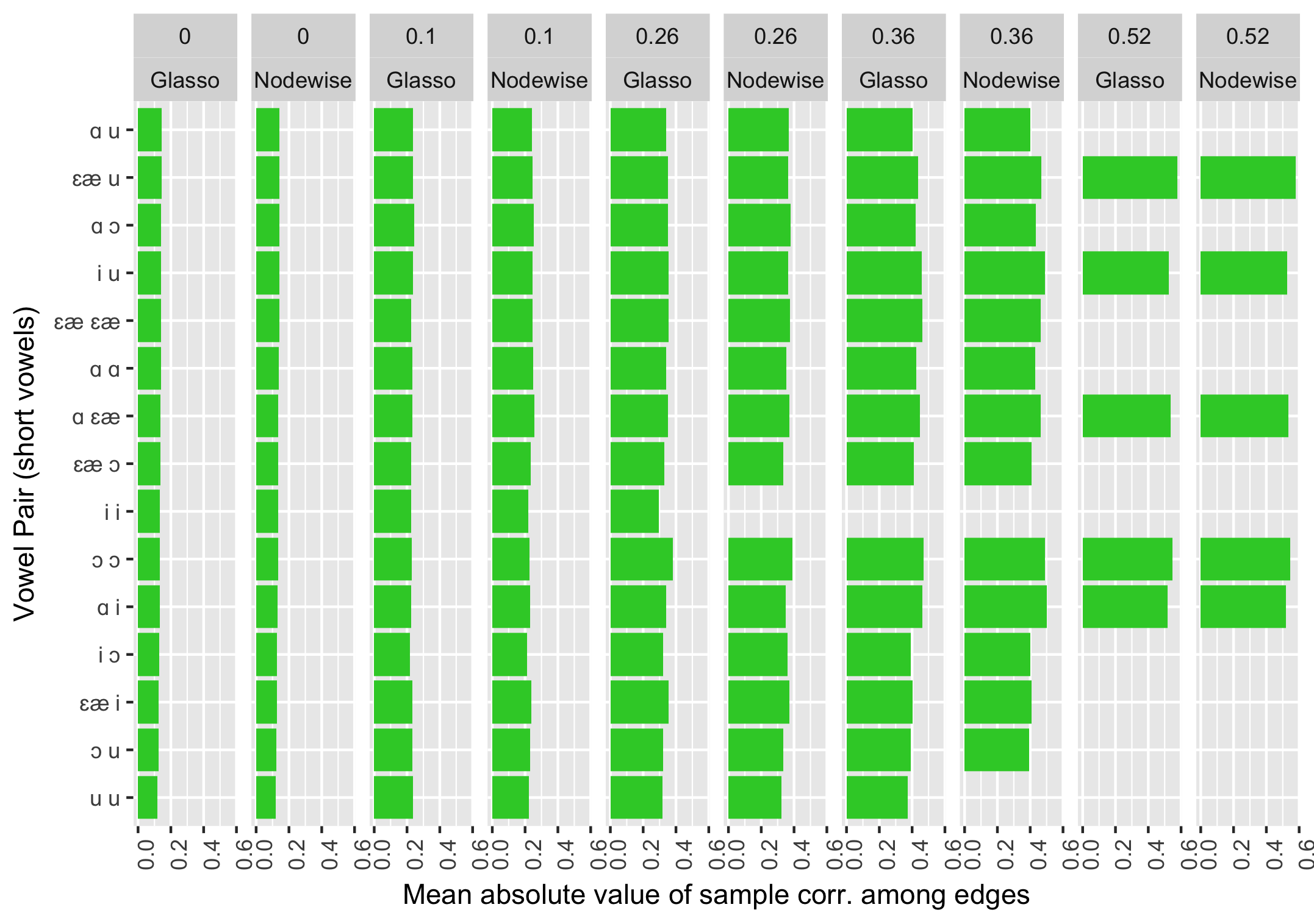
Figure 13: Bar chart of average sample correlation among edges for short vowels, estimated using Glasso and nodewise regression.

Figure 12 in the Appendix displays a bar chart of the fraction of edges between each pair of short vowels. By contrast to Figure 4, the edges appear to be uniformly distributed among vowel pairs. Figure 13 displays a bar chart for short vowels analogous to Figure 11. Hence for words with short vowels, edges appear to be driven more by the initial consonant than the vowel.

3.3 Conditional independence reveals initial consonants associate with vowel pronunciation

In Figure 6, we display the inverse correlation graph for all words, organized by initial consonant. The nodes are colored by category of the initial consonant: labial (pronounced with the lips), alveolar (pronounced with the tongue on the ridge behind the teeth), nasal (pronounced using the sinus cavity), and v/f (fricative, pronounced by partially obstructing the air). The Glasso penalty is $0.37$, followed by a threshold of $0.1$, and the nodewise regression penalty is $0.37$, followed by a threshold of $0.08$. The words are organized by initial consonant. Almost all of the edges are between group rather than within group; that is, almost all edges are between words starting with different consonants. In Figure 7, we present a high-level summary of this edge graph, by aggregating words with the same consonant into ``supernodes.'' Two supernodes are connected if there is an edge in Figure 6 between two words with the corresponding consonants, estimated by both Glasso and nodewise regression. This diagram holds for a particular choice of penalty and threshold. Figure 8 displays the Pearson correlations for word pairs that have edges in Figure 6.

The edges in the supernode diagram are associated with properties of words studied by linguists. Both m/n and w are continuously voiced consonants (i.e. they can be pronounced in a sustained way, with continuous vocal fold vibration). Figure 21 in the appendix displays a bar chart of the fraction of edges between each pair of onsets (initial consonants), for a sequence of Glasso penalty parameters. Even at a penatly of $0.43$, edges persist between words beginning with m/n and words beginning with w. Figure 20 in the appendix displays the inverse covariance graph for words with labial and alveolar initial consonants, estimated using Glasso with penalty $0.3$. At this penalty, the words starting with p and t are disconnected, whereas many edges remain between words starting with the other labial and alveolar consonants. The edges that remain are the same edges that are present in the supernode diagram, Figure 7. The leaf nodes are the fricative consonants v and w, whereas the labial b and alveolar t have more connections.

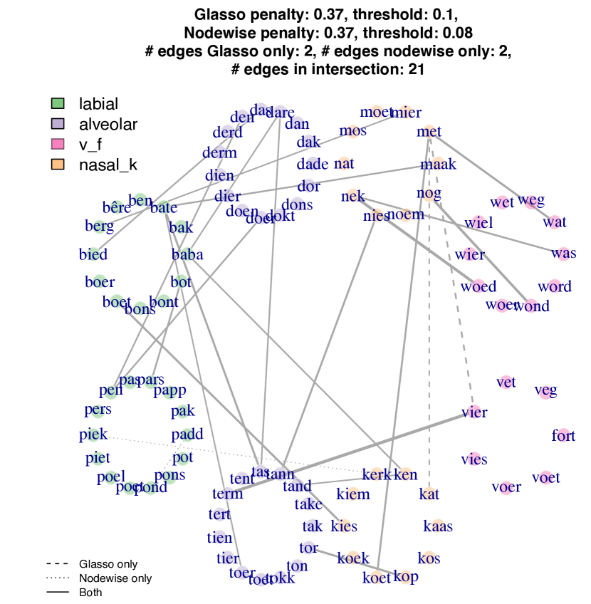
Figure 6: Inverse covariance graph of all words, comparing Glasso edges with nodewise regression edges.

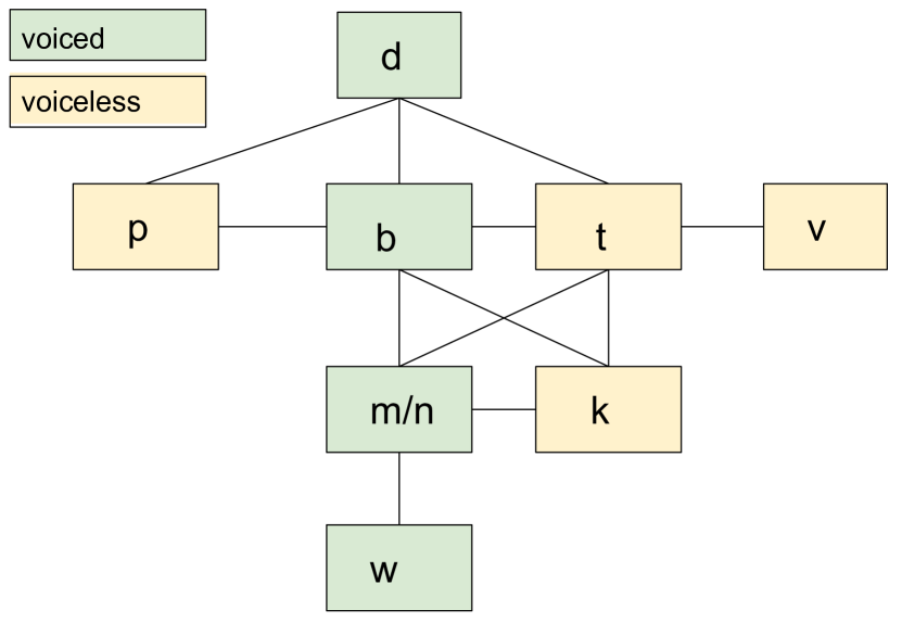
Figure 7: Diagram displaying connectivity among consonants, providing a higher-level representation of Figure 6 by combining nodes within a consonant type into ``supernodes.'' Two nodes are connected in this diagram if there is an edge estimated by both Glasso and nodewise regression between words with the corresponding initial consonants in Figure 6.

Word One	Word Two	Pearson Correlation
kop	tor	$0.53$
nog	wond	$0.56$
den	pen	$0.49$
baba	ken	$-0.49$
bate	maak	$0.50$
bate	tas	$0.52$
bate	toer	$-0.48$
berg	mier	$0.48$
bied	das	$0.49$
boet	kies	$0.60$
bot	pars	$0.50$
dare	baba	$0.48$

Word One	Word Two	Pearson Correlation
doer	pen	$0.50$
kat	met	$-0.48$
ken	tand	$0.48$
kerk	piek	$0.45$
koet	met	$0.51$
met	vier	$0.52$
met	wat	$0.53$
nek	was	$0.51$
nek	woed	$0.58$
padd	pond	$0.46$
term	vier	$0.60$

Figure 8: Word-word pearson correlations for words with edges in Figure 6.

3.4 Heteroscedasticity and nonstationary autocorrelation indicate heterogeneity over time

Since the pitch curves are smooth, strong local correlations along the time axis are expected. The time-time dependence structure is informative in that it provides a characterization of the variance of the pitch curves as a function of time, and reveals the extent to which local dependencies decay.

The time-time covariance matrices for each word group (labial, alveolar, nasal, fricative) shown in Section C.3 of the Appendix indicate that the variance increases over time; that is, the pitch exhibits greater variability at the end of the word utterance than at the beginning. This indicates that speech may be more constrained at the beginning of a word token than at the end. The correlation matrices are approximately banded, and essentially all pairwise correlations are above $0.5$. In some cases the correlations decay faster at the end of the utterance than at the beginning.

The diagonal entries of the inverse covariance matrix reflect the residual variances of each time point when regressed on the other other time points; a small diagonal entry corresponds to large residual variance. For each of the word groups, the diagonal entries of the precision matrix are decreasing in time, also consistent with the early portion of the utterance being more constrained and predictable than the later portion of the utterance.

In Table 1, we report metrics related to the Glasso estimate of the time-time correlation matrix. Based on the estimated effective sample using all words ($n(r)=4$, $n(w)=93$, $n(s)=20$), using the identity matrix for the word-word covariance, the theoretical penalty is $\sqrt{\log(n(w))/(n(s)*n(r)*n(w))}=0.03$. In practice, due to dependence on the other axis, one should use a larger penalty when estimating the time-time inverse covariance. The similar time-time edge structure for the word groups motivates pooling across the word groups to estimate a common time-time inverse correlation structure.

4 Conclusion

Using recently developed methods for tensor data with multi-way dependence, we show that word-word edges in an Afrikaans pitch curve data set are associated with natural word attributes of interest to linguists. This data analysis suggests that the notion of conditional independence and tools of graphical modeling, which have proved useful in other scientific fields are also useful in the field of phonetics. In particular, long vowel edges are driven by whether the vowel is pronounced at the front of the mouth or back of the mouth. A future research question of interest is whether the patterns observed here hold in other languages.

Acknolwedgments

We thank Will Styler for very delightful discussions of our initial findings as detailed in this report.

Appendix A Outline of supplement

Section A.1 displays the International Phonetic Alphabet (IPA) representation for Afrikaans words used in Coetzee et al. (2018). Section B discusses word-word inverse covariance estimation and graphical modeling. Section B.1 presents an inverse covariance graph and trial residualized pitch curves for words with long vowels, as well as bar charts and Pearson correlation tables summarizing the edges for long and short vowels. Section B.2 demonstrates that for words starting with labial and alveolar consonants, ``p'' and ``t'' become disconnected in the graphical model for sufficiently high penalty parameter. Section B.3 displays bar charts of the fraction of edges and Pearson correlation between each pair of initial consonants. Section B.4 shows that edges for words with short vowels are associated with initial consonant (onset) and final consonant (coda). Further visualizing these edges, Section B.5 displays the graphical model for all $93$ words, with each plot containing a subgraph consisting of two word categories (among labial, alveolar, nasal/k, and fricative) with a penalty of $0.32$ and threshold of $0.16$, and Section B.6 displays analogous plots with a penalty of $0.26$ and threshold $0.08$. Section C.3 discusses estimation of the time-time covariance and inverse covariance matrices, and compares time-time edges estimated using different subsets of words.

A.1 IPA representation of Afrikaans words

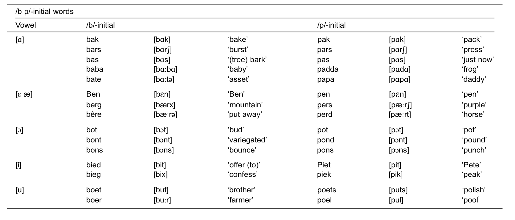
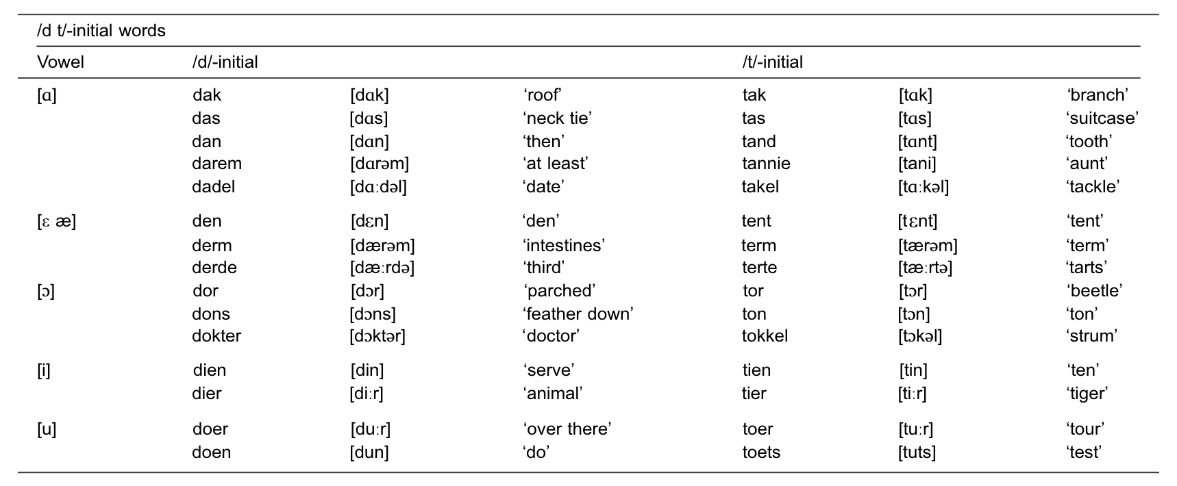
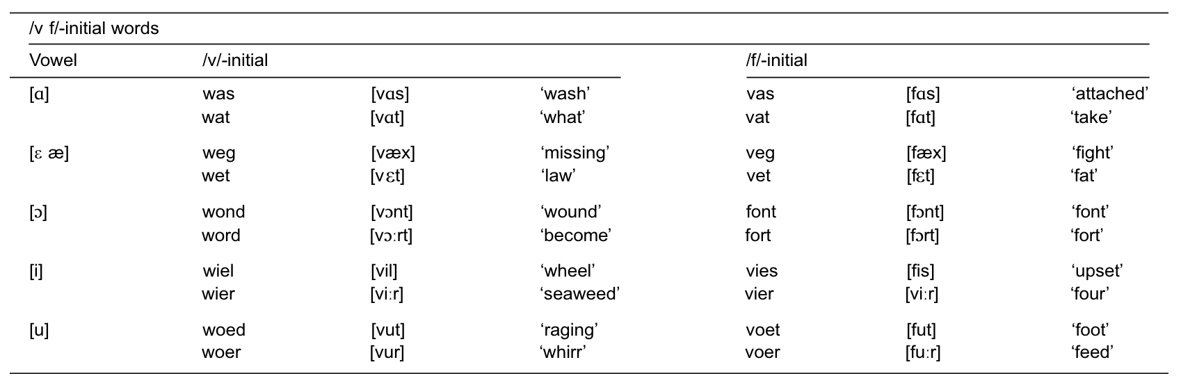
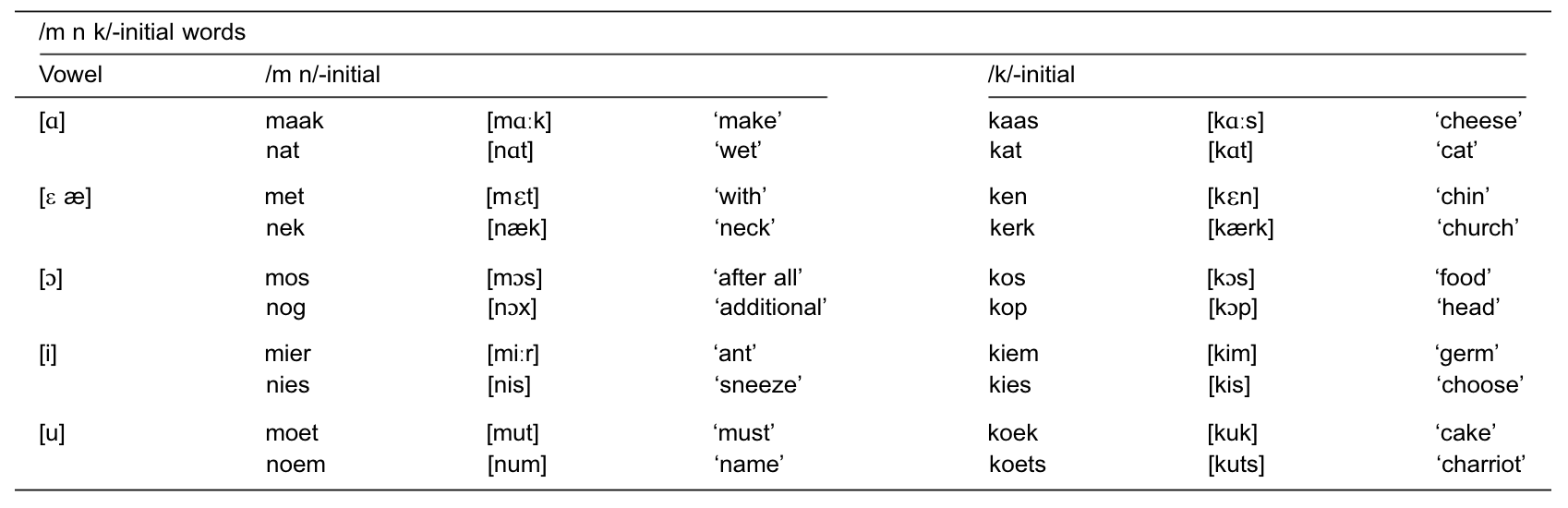
Figure 9: From Appendix A of Coetzee et al. (2018)

Appendix B Word-word graphical models and inverse correlation estimation

Word Group	Avg. node degree	# edges	$\text{tr}(B)/\lVert B\rVert_{F}$	$\lVert B\rVert_{2}$
All words ($93$ words)	$9.3$	$88$	$4.05$	$5.0$
Labial ($26$ words)	$9.5$	$90$	$4.05$	$5.0$
Alveolar ($30$ words)	$9.8$	$93$	$4.05$	$5.0$
Nasal words ($20$ words)	$9.8$	$93$	$4.07$	$5.0$
vf words ($17$ words)	$8.4$	$80$	$4.03$	$5.1$

Table 1: Metrics related to estimate of time-time correlation matrix.

B.1 Analyzing edges related to long vowels

Word One	Word Two	Pearson Correlation
bate	maak	$0.50$
kaas	maak	$0.41$
baba	tier	$0.37$
bate	maak	$0.50$
bate	toer	$-0.48$
boer	kaas	$0.28$
boer	mier	$0.36$
bêre	tert	$0.35$
bêre	vier	$0.33$
bate	kaas	$0.22$
dade	maak	$0.32$
derd	wier	$0.27$
dier	kaas	$0.35$
doer	voer	$0.26$
doer	word	$0.36$
kaas	tert	$0.28$
tert	vier	$0.30$
wier	tier	$0.35$

Table 2: Word-word Pearson correlations.

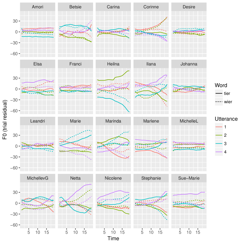
Figure 17: Trial residual pitch curves for the words wier and tier.

B.2 Labial and alveolar words

In Figures 18, 19, and 20 we show the inverse covariance graph estimated using a sequence of Glasso penalty parameters, with a threshold of $0.1$. For small penalty values, words of all four initial consonants (b, d, p, t) are densely connected. As the penalty increases the edges between words beginning with p and t drop off.

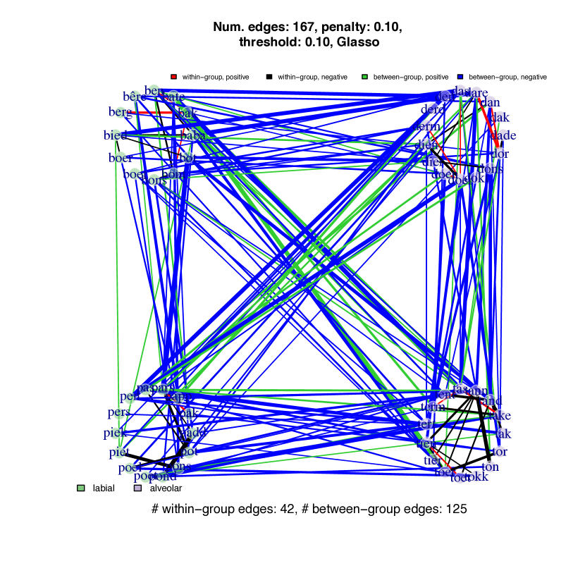
Figure 18: Inverse covariance graph of labial and alveolar words Glasso with a peanlty of $0.1$ and a threshold of $0.1$.

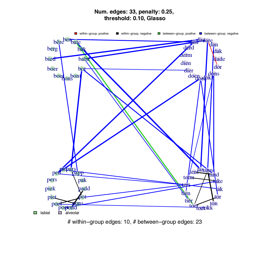
Figure 19: Inverse covariance graph of labial and alveolar words Glasso with a peanlty of $0.25$ and a threshold of $0.1$.

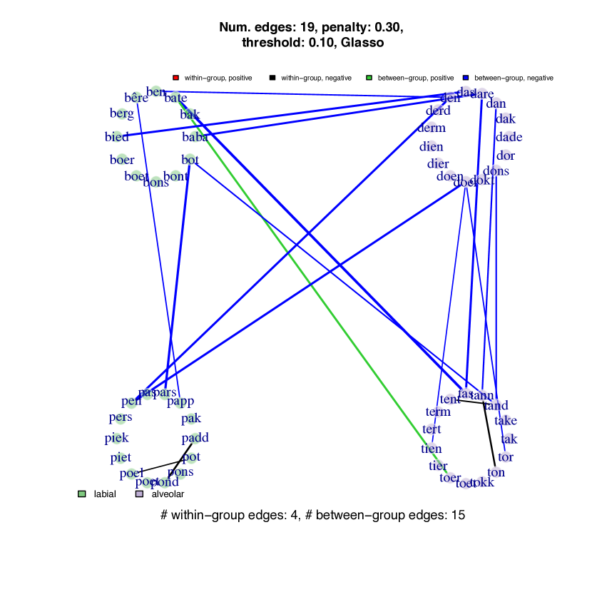
Figure 20: Inverse covariance graph of labial and alveolar words Glasso with a peanlty of $0.3$ and a threshold of $0.1$.

B.3 Initial consonant connectivities

Figure 21 displays a bar chart of the fraction of edges between each pair of onsets (i.e. initial consonants), for a sequence of Glasso penalty parameters. When counting edges, the ``m'' and ``n'' are treated as a single consonant, as are the consonants ``v'' and ``f''. Figure 22 displays the mean Pearson correlation among edges in the for each consonant pair.

Figure 21: Fraction of edges between each pair of initial consonants as we vary the Glasso penalty.

Figure 22: Mean absolute value of Pearson correlation among edges between each pair of initial consonants.

B.4 Associations between short vowel edges and word attributes

Figure 23: Bar chart of fraction of edges between each pair of onsets (initial consonants) for words with short vowels, estimated using Glasso and nodewise regression.

Figure 24: Bar chart of fraction of edges between each pair of first codas (consonant after the vowel) for words with short vowels, estimated using Glasso and nodewise regression.

Figure 25: Bar chart of fraction of edges between each pair of last codas (last consonant of the syllable) for words with short vowels, estimated using Glasso and nodewise regression.

Figure 26: Bar chart of average sample correlation between words with edges for each pair of last codas, estimated using Glasso and nodewise regression.

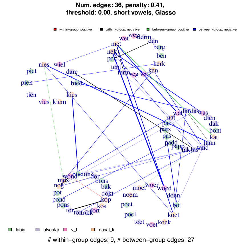
Figure 28: Inverse covariance graph of words with short vowels, estimated using Glasso regression, organized by vowel.

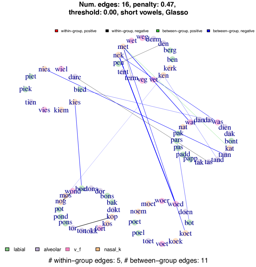
Figure 29: Inverse covariance graph of words with short vowels, estimated using Glasso regression, organized by vowel.

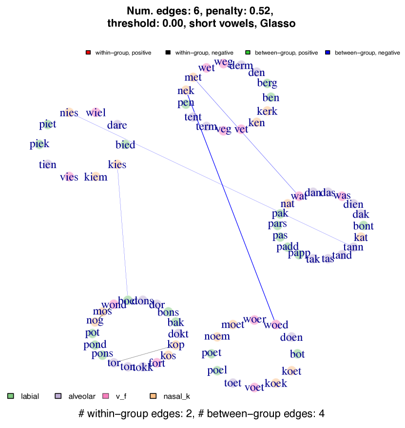
Figure 30: Inverse covariance graph of words with short vowels, estimated using Glasso regression, organized by vowel.

B.5 Comparing Glasso and nodewise regression graphs for pairs of word groups

We display inverse correlation graphs between each pair of word groups (labial, alveolar, nasal, and vf). Glasso and nodewise regression were run on all the words; in the following figures, we visualize subgraphs of the full graph. The line type indicates whether the edge appears in both the Glasso and nodewise regression graphs or in just one of the two. Both methods are run with a penalty of $0.32$ and threshold of $0.16$. We see that the edges are similar between the methods, but with more edges for Glasso than nodewise regression. In Section B.6 of the Appendix, we display analogous plots with a penalty of $0.26$ and threshold $0.08$.

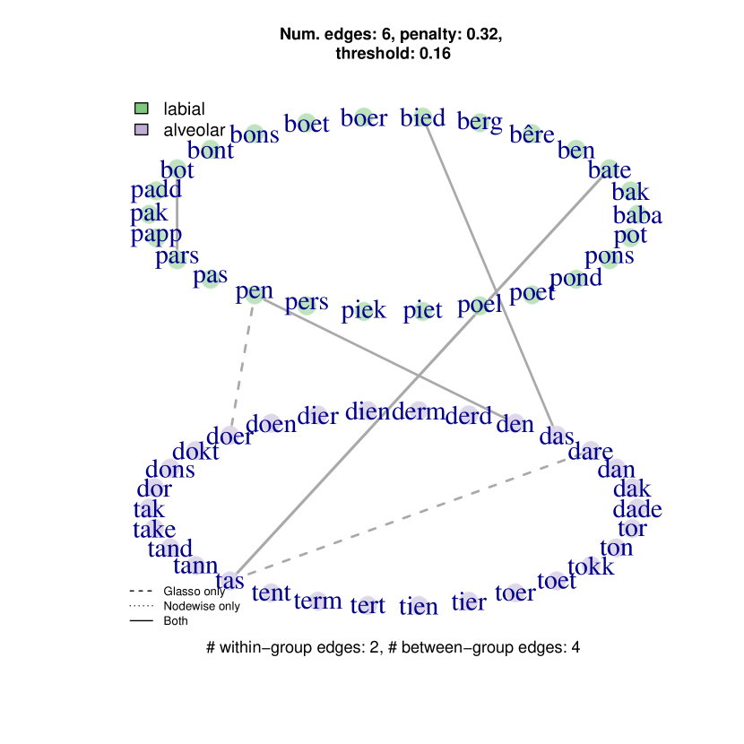
Figure 31: Inverse covariance graph of labial and alveolar words. This graph displays a subgraph of a graph for all $93$ words, estimated using Glasso and nodewise regression with thresholding.

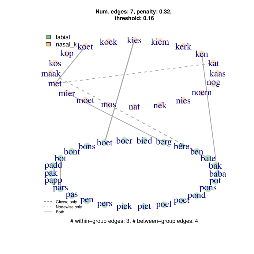
Figure 32: Inverse covariance graph of labial and nasal words. This graph displays a subgraph of a graph for all $93$ words, estimated using Glasso and nodewise regression with thresholding.

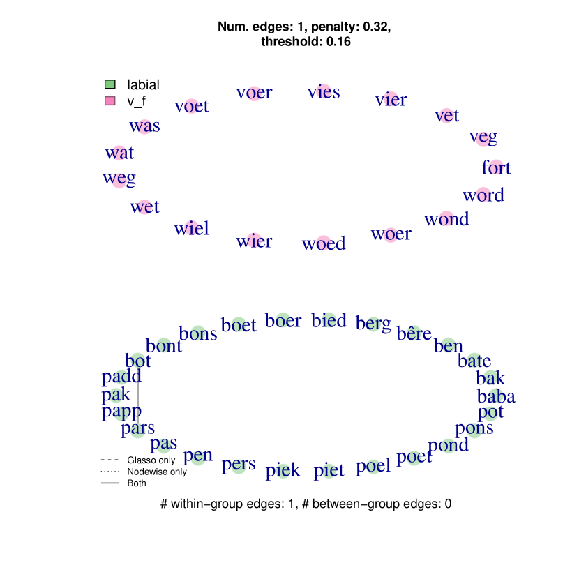
Figure 33: Inverse covariance graph of labial and vf words. This graph displays a subgraph of a graph for all $93$ words, estimated using Glasso and nodewise regression with thresholding.

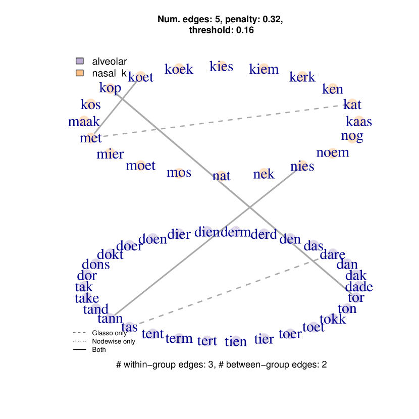
Figure 34: Inverse covariance graph of alveolar and nasal words. This graph displays a subgraph of a graph for all $93$ words, estimated using Glasso and nodewise regression with thresholding.

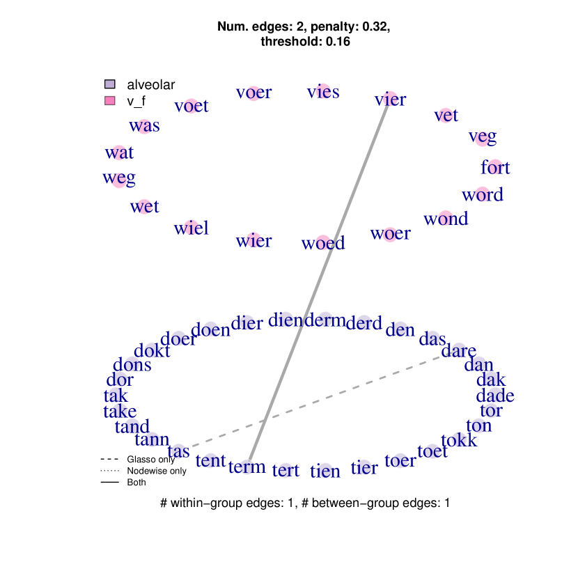
Figure 35: Inverse covariance graph of alveolar and vf words. This graph displays a subgraph of a graph for all $93$ words, estimated using Glasso and nodewise regression with thresholding.

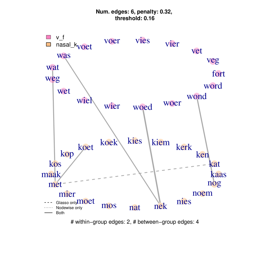
Figure 36: Inverse covariance graph of nasal and vf. This graph displays a subgraph of a graph for all $93$ words, estimated using Glasso and nodewise regression with thresholding.

B.6 Edge graphs comparing Glasso and nodewise regression, for each pair of word groups (labial, alveolar, nasal, vf)

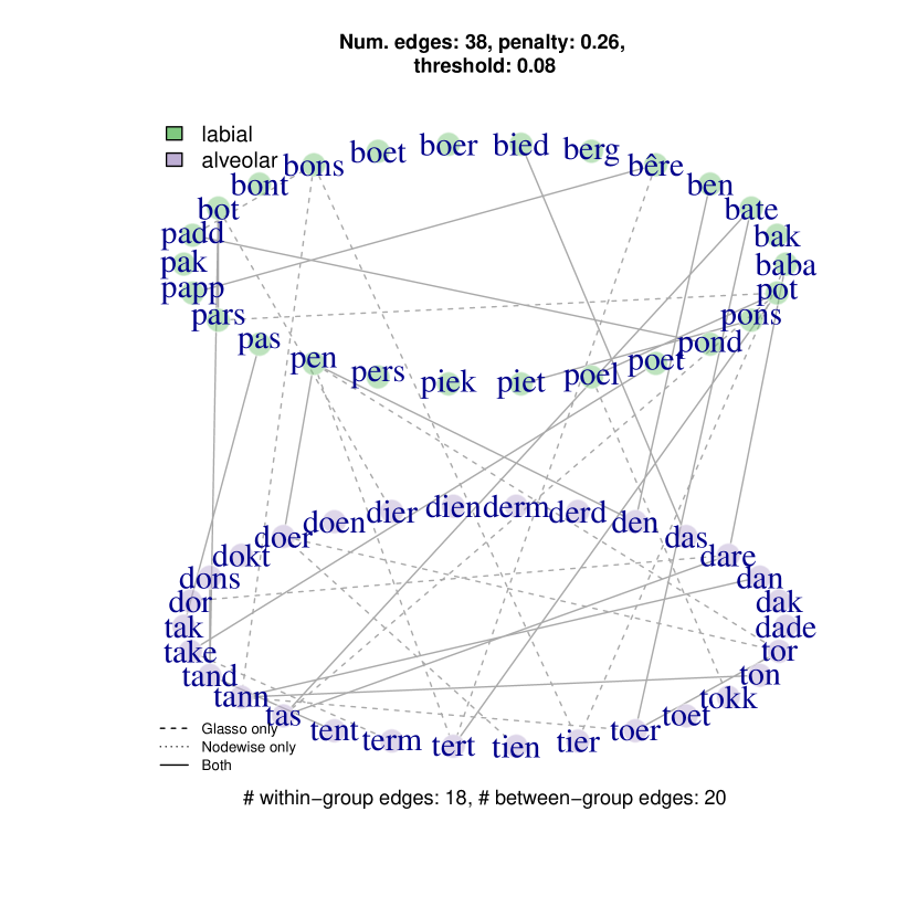
Figure 37: Inverse covariance graph of labial and alveolar words. This graph displays a subgraph of a graph for all $93$ words, estimated using Glasso and nodewise regression with thresholding.

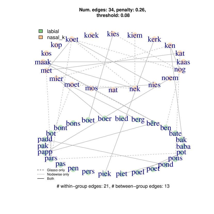
Figure 38: Inverse covariance graph of labial and nasal words. This graph displays a subgraph of a graph for all $93$ words, estimated using Glasso and nodewise regression with thresholding.

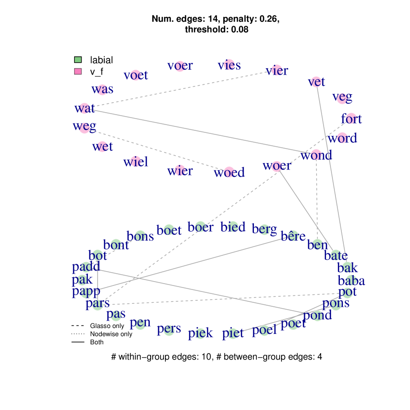
Figure 39: Inverse covariance graph of labial and vf words. This graph displays a subgraph of a graph for all $93$ words, estimated using Glasso and nodewise regression with thresholding.

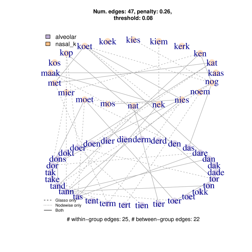
Figure 40: Inverse covariance graph of alveolar and nasal words. This graph displays a subgraph of a graph for all $93$ words, estimated using Glasso and nodewise regression with thresholding.

Figure 41: Inverse covariance graph of alveolar and vf words. This graph displays a subgraph of a graph for all $93$ words, estimated using Glasso and nodewise regression with thresholding.

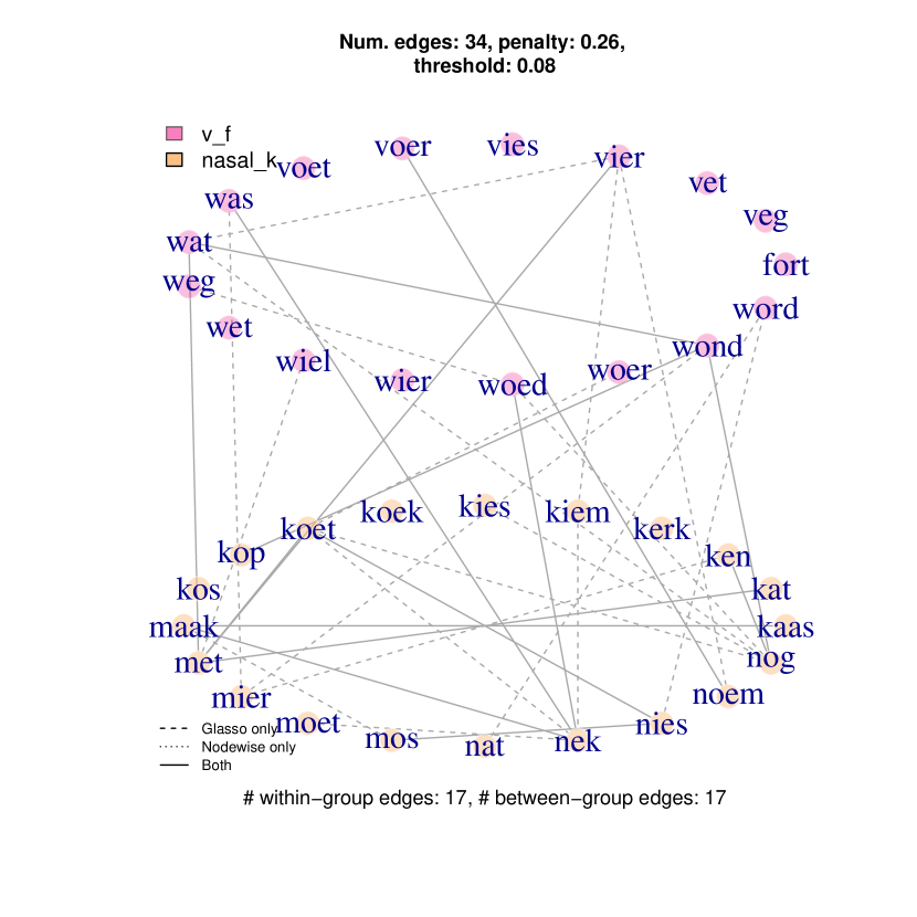
Figure 42: Inverse covariance graph of nasal and vf words. This graph displays a subgraph of a graph for all $93$ words, estimated using Glasso and nodewise regression with thresholding.

Appendix C Time-time inverse covariance modeling

C.1 Time-time and word-word correlation and covariance

Figure 43 displays sample covariance, sample correlation, Glasso covariance, Glasso inverse covariance, Glasso correlation, and Glasso inverse correlation for the labial words. Glasso is run using a penalty five times that of of the theoretical value. In Section C.3 of the Supplement, analogous figures are shown for the other word groups.

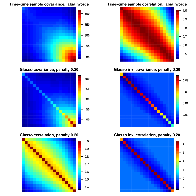
Figure 43: Time-time sample covariance (top left), sample correlation (top right), Glasso covariance (middle left), Glasso inverse covariance (middle right), Glasso correlation (bottom left), and Glasso inverse correlation (bottom right), for words beginning with a labial consonant. The sample covariance is calculated as in (4), and the Glasso penalty parameter is chosen as five times the value of (8).

C.2 Comparison of time inverse covariance graphs for each pair of word groups

For each pair of word groups, we compare the time-time inverse correlation graphs, by taking intersections and set differences. We threshold each graph down to $70$ edges. In each graph, nodes are connected to approximately five nearest neighbors on each side. The time-time edges are similar among the word groups; that is, most of the nodes are in the intersections of the graphs. This suggests that we can consider using a combined time-time inverse covariance matrix pooling over the words to decorrelate along the time axis, potentially improving the word-word covariance estimates, discussed in Zhou (2014).

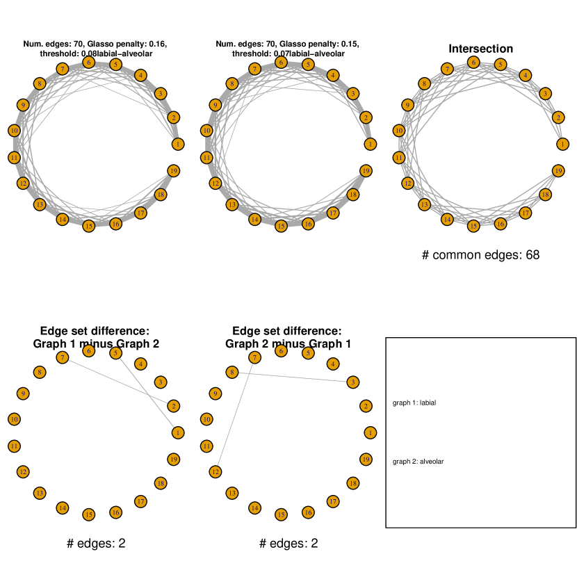
Figure 44: Time-time inverse covariance graphs for labial and alveolar words, as well as graph intersection and set differences. The inverse correlation matrices are thresholded so that $70$ edges remain in each word group.

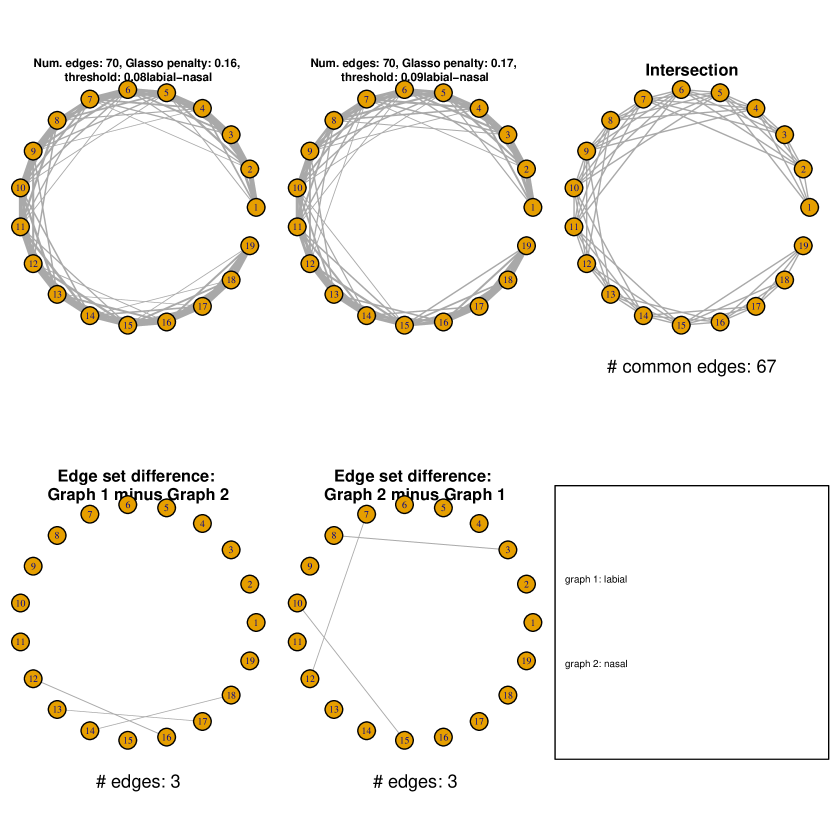
Figure 45: Time-time inverse covariance graphs for labial and nasal words, as well as graph intersection and set differences.

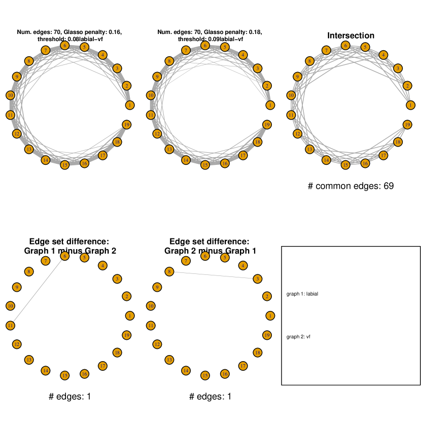
Figure 46: Time-time inverse covariance graphs for labial and vf words, as well as graph intersection and set differences.

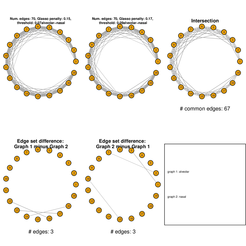
Figure 47: Time-time inverse covariance graphs for alveolar and nasal words, as well as graph intersection and set differences.

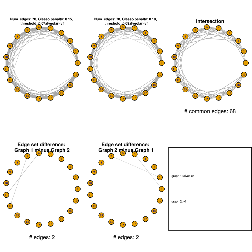
Figure 48: Time-time inverse covariance graphs for alveolar and vf words, as well as graph intersection and set differences.

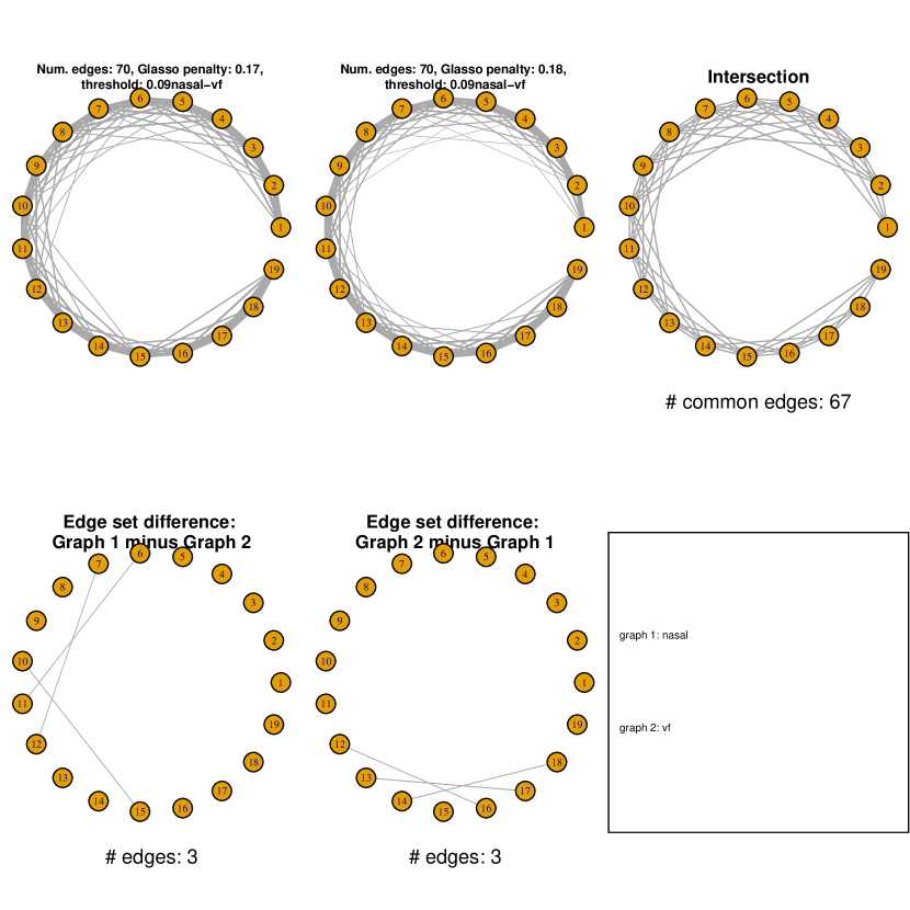
Figure 49: Time-time inverse covariance graphs for nasal and vf words, as well as graph intersection and set differences.

C.3 Time-time covariance, correlation, inverse covariance, and inverse correlation

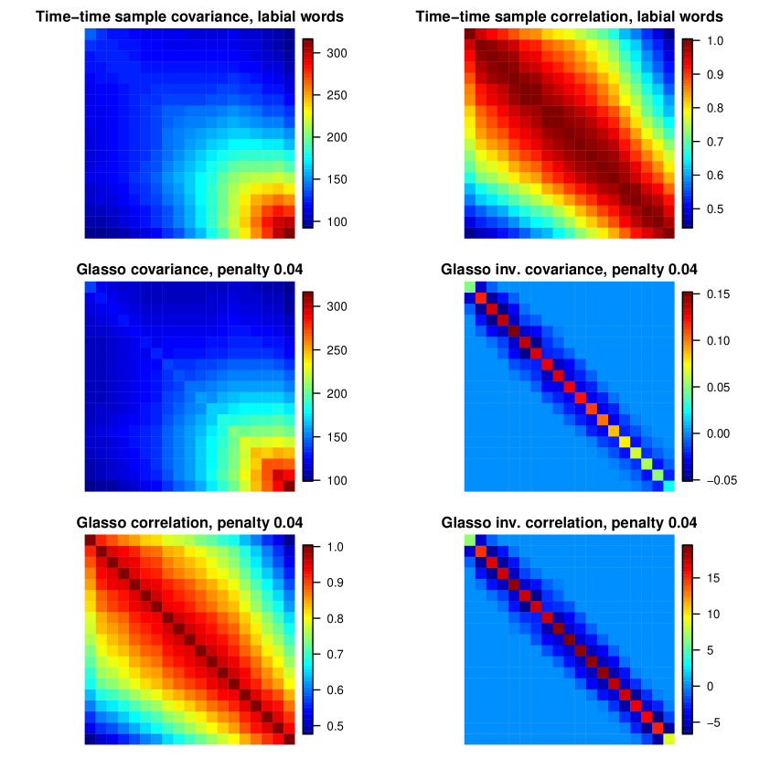
Figure 50: Time-time sample covariance (top left), sample correlation (top right), Glasso covariance (middle left), Glasso inverse covariance (middle right), Glasso correlation (bottom left), and Glasso inverse correlation (bottom right), for words beginning with a labial consonant. The sample covariance is calculated as in (4), and the Glasso penalty parameter is chosen as in (8).

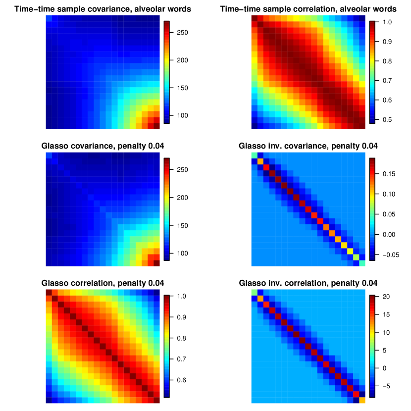
Figure 51: Time-time sample covariance (top left), sample correlation (top right), Glasso covariance (middle left), Glasso inverse covariance (middle right), Glasso correlation (bottom left), and Glasso inverse correlation (bottom right), for words beginning with an alveolar consonant. The sample covariance is calculated as in (4), and the Glasso penalty parameter is chosen as in (8).

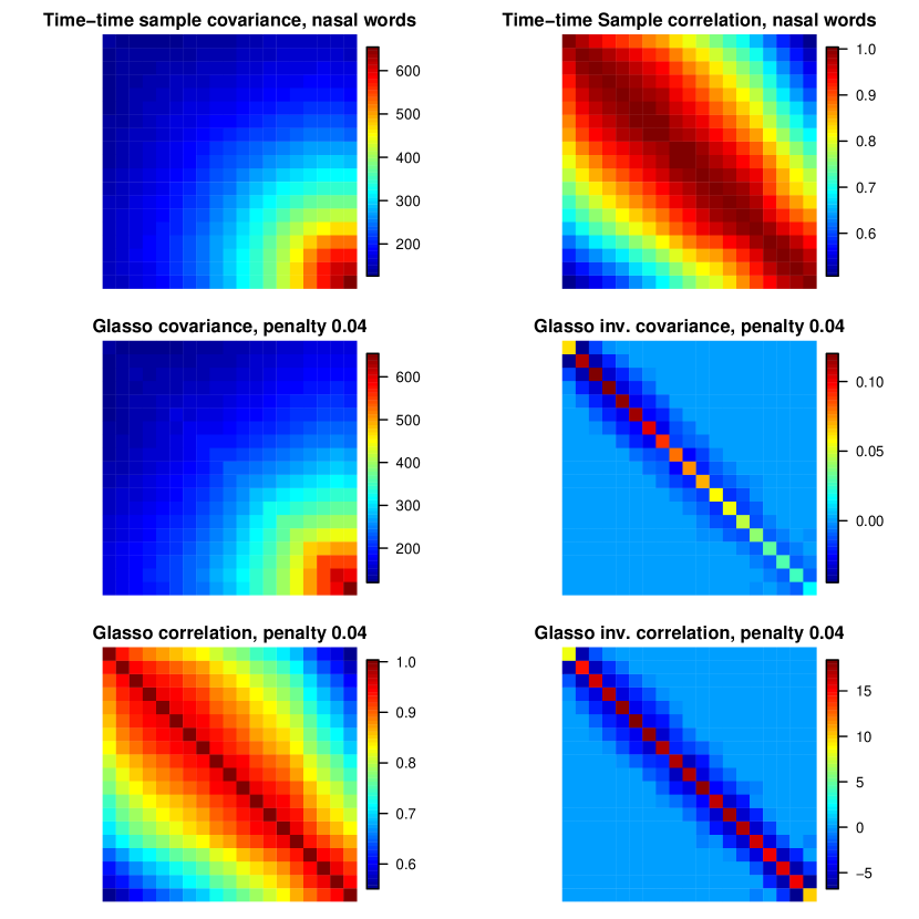
Figure 52: Time-time sample covariance (top left), sample correlation (top right), Glasso covariance (middle left), Glasso inverse covariance (middle right), Glasso correlation (bottom left), and Glasso inverse correlation (bottom right), for words beginning with a nasal consonant. The sample covariance is calculated as in (4), and the Glasso penalty parameter is chosen as in (8).

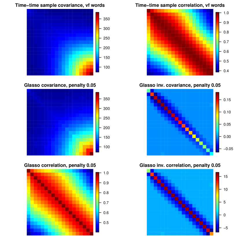
Figure 53: Time-time sample covariance (top left), sample correlation (top right), Glasso covariance (middle left), Glasso inverse covariance (middle right), Glasso correlation (bottom left), and Glasso inverse correlation (bottom right), for words beginning with a vf consonant. The sample covariance is calculated as in (4), and the Glasso penalty parameter is chosen as in (8).

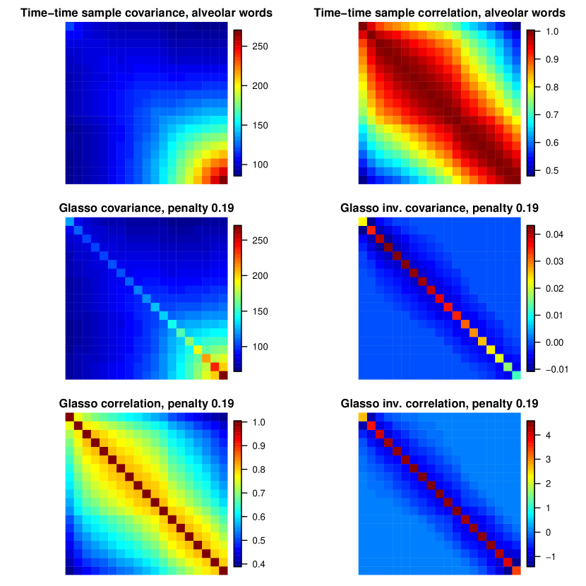
Figure 54: Time-time sample covariance (top left), sample correlation (top right), Glasso covariance (middle left), Glasso inverse covariance (middle right), Glasso correlation (bottom left), and Glasso inverse correlation (bottom right), for words beginning with an alveolar consonant. The sample covariance is calculated as in (4), and the Glasso penalty parameter is chosen as five times the value of (8).

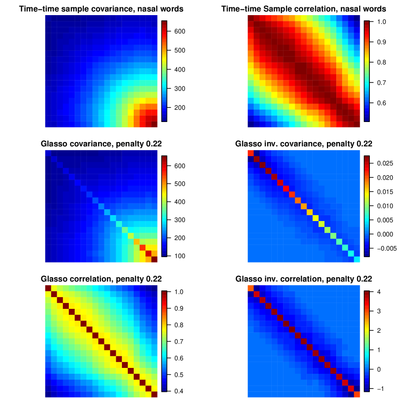
Figure 55: Time-time sample covariance (top left), sample correlation (top right), Glasso covariance (middle left), Glasso inverse covariance (middle right), Glasso correlation (bottom left), and Glasso inverse correlation (bottom right), for words beginning with a nasal consonant. The sample covariance is calculated as in (4), and the Glasso penalty parameter is chosen as five times the value of (8).

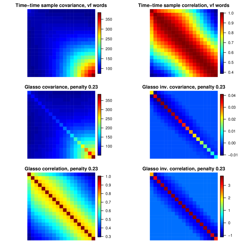
Figure 56: Time-time sample covariance (top left), sample correlation (top right), Glasso covariance (middle left), Glasso inverse covariance (middle right), Glasso correlation (bottom left), and Glasso inverse correlation (bottom right), for words beginning with a vf consonant. The sample covariance is calculated as in (4), and the Glasso penalty parameter is chosen as five times the value of (8).

References

- Baayen et al. (2008) Baayen, R. H., Davidson, D. J. and Bates, D. M. (2008). Mixed-effects modeling with crossed random effects for subjects and items. Journal of memory and language 59 390–412.
- Boersma (1993) Boersma, P. (1993). Accurate short-term analysis of the fundamental frequency and the harmonics-to-noise ratio of a sampled sound. In Proceedings of the institute of phonetic sciences, vol. 17. Amsterdam.
- Chetouani et al. (2009) Chetouani, M., Mahdhaoui, A. and Ringeval, F. (2009). Time-scale feature extractions for emotional speech characterization. Cognitive Computation 1 194–201.
- Coetzee et al. (2018) Coetzee, A. W., Beddor, P. S., Shedden, K., Styler, W. and Wissing, D. (2018). Plosive voicing in afrikaans: Differential cue weighting and tonogenesis. Journal of Phonetics 66 185–216.
- Hanson (2009) Hanson, H. M. (2009). Effects of obstruent consonants on fundamental frequency at vowel onset in english. The Journal of the Acoustical Society of America 125 425–441.
- Hirst (2011) Hirst, D. J. (2011). The analysis by synthesis of speech melody: from data to models. Journal of speech Sciences 1 55–83.
- Houde and Jordan (1998) Houde, J. F. and Jordan, M. I. (1998). Adaptation in speech motor control. In Advances in neural information processing systems.
- Iriondo et al. (2009) Iriondo, I., Planet, S., Socoró, J.-C., Martínez, E., Alías, F. and Monzo, C. (2009). Automatic refinement of an expressive speech corpus assembling subjective perception and automatic classification. Speech Communication 51 744–758.
- Kalaitzis et al. (2013) Kalaitzis, A., Lafferty, J., Lawrence, N. and Zhou, S. (2013). The bigraphical lasso. In Proceedings of The 30th International Conference on Machine Learning ICML-13.
- Loh and Wainwright (2012) Loh, P. and Wainwright, M. (2012). High-dimensional regression with noisy and missing data: Provable guarantees with nonconvexity. The Annals of Statistics 40 1637–1664.
- Meinshausen and Bühlmann (2006) Meinshausen, N. and Bühlmann, P. (2006). High dimensional graphs and variable selection with the Lasso. Annals of Statistics 34 1436–1462.
- Shami and Verhelst (2007) Shami, M. and Verhelst, W. (2007). An evaluation of the robustness of existing supervised machine learning approaches to the classification of emotions in speech. Speech Communication 49 201–212.
- Sheikhan et al. (2013) Sheikhan, M., Bejani, M. and Gharavian, D. (2013). Modular neural-svm scheme for speech emotion recognition using anova feature selection method. Neural Computing and Applications 23 215–227.
- Wissing (2012) Wissing, D. (2012). Integrasie van artikulatoriese en akoestiese eienskappe van vokale:'n beskrywingsraamwerk: geesteswetenskappe. Litnet Akademies:'n Joernaal vir die Geesteswetenskappe, Natuurwetenskappe, Regte en Godsdienswetenskappe 9 701–743.
- Yuan (2010) Yuan, M. (2010). High dimensional inverse covariance matrix estimation via linear programming. Journal of Machine Learning Research 11 2261–2286.
- Zhou (2010) Zhou, S. (2010). Thresholded lasso for high dimensional variable selection and statistical estimation. Tech. rep., Department of Statistics, University of Michigan.
- Zhou (2014) Zhou, S. (2014). Gemini: Graph estimation with matrix variate normal instances. Annals of Statistics 42 532–562.
- Zhou et al. (2011a) Zhou, S., Rütimann, P., Xu, M. and Bühlmann, P. (2011a). High-dimensional covariance estimation based on gaussian graphical models. Journal of Machine Learning Research 12 2975–3026.
- Zhou et al. (2011b) Zhou, S., Rütimann, P., Xu, M. and Bühlmann, P. (2011b). High-dimensional covariance estimation based on Gaussian graphical models. Journal of Machine Learning Research 12 2975–3026.