Umbilic Points on the Finite and Infinite Parts of Certain Algebraic Surfaces

Abstract

The global qualitative behaviour of fields of principal directions for the graph of a real valued polynomial function $f$ on the plane is studied. We determine and analyze the projective extension of these fields and show that it is defined by an analytic quadratic form on the whole unit 2-sphere. We prove that every umbilic point at infinity of this extension has a Poincaré-Hopf index equal to 1/2 and the topological type of a Lemon or a Monstar. As a consequence of these results we provide a Poincaré-Hopf type formula for the graph of $f$ pointing out that, if all umbilics are isolated, the sum of all indices of the principal directions at its umbilic points only depends upon the number of real linear factors of the homogeneous part of highest degree of $f$. A similar analysis is carried out in the case that $f$ is a homogeneous polynomial.

Keywords: umbilic points at infinity; real polynomials; fields of principal directions.

Mathematics Subject classification: 53C12, 53A05, 34K32, 53A20

1 Introduction

For any oriented smooth surface in real Euclidean 3-space, the eigenspaces of its second fundamental form define two orthogonal line fields, called fields of principal directions, whose singularities are the umbilics of the surface. The study of the fields of principal directions and the principal lines of a smooth surface dates back to Euler, Darboux [5], Monge [15] and Cayley [4], amongst others. An umbilic is characterized by the fact that its principal curvatures are equal. Moreover, to each isolated umbilic can be attached the index of either one of the two fields. This index is of the form ${n}/{2}$, with $n\in\mathbb{Z}$. When such a surface is generic, the behaviour of the principal lines in the neighbourhood of an umbilic can only be one of three Darbouxian types: Lemon, Monstar and Star [13] (see Fig. 1) with Poincaré-Hopf index $\frac{1}{2},\frac{1}{2},-\frac{1}{2}$, respectively. For topological reasons, if all of the umbilics are isolated, the sum over all half-integer indices of the fields of principal directions at its umbilic points equals the Euler characteristic of the surface.

Fig. 1: Darbouxian points

The study of umbilic points at infinity of a surface has been developed from various perspectives previously. In the case of smooth surfaces, V. Toponogov analyzes in [19], surfaces $S$ homeomorphic to a plane which are complete and convex. In terms of the principal curvatures $\kappa_{1},\kappa_{2}$ of $S$ he states the conjecture:

“on a complete convex surface $S$ homeomorphic to a plane, the equality

inf_p∈S $|k_{2}(p)-k_{1}(p)|=0$ holds”.

If there are no finite umbilic points, this can be taken to mean that there must be an umbilic point at infinity. In the same paper, he proves this conjecture under some additional hypotheses. We remark that after a straightforward calculation, this equality can be verified for any surface that is given as the graph of a real polynomial.

Another instance of umbilic points at infinity in the smooth case is the study, carried out by R. Garcia and J. Sotomayor in [7], on stable patterns of the nets of principal curvature lines on surfaces embedded in Euclidean 3-space near their end points, at which the surfaces tend to infinty. The research just cited is an extension of the work by the same authors [6] and devoted to the analysis at infinity of the principal curvature nets of smooth algebraic surfaces in real Euclidean 3-space. The surfaces discussed in [6] do not cover those studied in this paper as the former consider surfaces having a smooth projective closure while those studied in this paper are singular at infinity.

In the particular case of a surface given by the graph of a homogeneous polynomial $f\in\mathbb{R}[x,y]$, the study of the index of the umbilic point that appears after the one-point compactification of the surface with the point at infinity, was carried out by N. Ando in [1].

On the other hand, and in a broader context, there is the investigation of singular points, their Poincaré-Hopf index and topological type, that arise at infinity as a result of the projective extension of a quadratic differential form on the plane. In [10] V. Guíñez considers the set ${\cal F}_{m}$ of positive quadratic forms

$$\omega=a(x,y)\,dy^{2}+b(x,y)\,dxdy+c(x,y)\,dx^{2},$$

such that $a,b,c\in\mathbb{R}[x,y]$ are polynomials of degree at most $m$, the function $\,b^{2}-4ac\,$ is non-negative at every point of the $xy$-plane, and $(b^{2}-4ac)^{-1}(0)=a^{-1}(0)\cap b^{-1}(0)\cap c^{-1}(0)$. For a generic form $\omega\in{\cal F}_{m}$, he studies the projective extension of $\omega$ and proves, amongst other things, that the topological behavior of these foliations in a neighborhood of a singular point at infinity is a Monstar or a Star (Remark 2.9 of [10]).

In this paper, we study the global qualitative behaviour of fields of principal directions for the graph of a polynomial $f\in\mathbb{R}[x,y]$. This study is carried out through the analysis of the projective extension of the quadratic form $\operatorname{\cal{PD}}$ that defines the fields of principal directions of the surface, and the singular points that appear on it. It is worth emphasizing that even though the quadratic form $\operatorname{\cal{PD}}$ belongs to the set ${\cal F}_{3n-4}$, it is not a generic form of those analyzed in [10] as the polynomial expression determining the singular points at infinity of the projective extension of $\operatorname{\cal{PD}}$ vanishes at every point on the equator of the unit sphere. Nevertheless, by using Euler’s Lemma we obtain a non-degenerate form on the equator.

In what follows we begin by providing an analytic quadratic form $\Phi$ defined on the whole sphere that describes the projective extension of the form $\operatorname{\cal{PD}}$. The two solution fields of this form, $\mathbb{Y}_{1},\mathbb{Y}_{2}$, being restricted to the upper or lower open hemispheres, are diffeomorphic to the fields of principal directions, in Theorem 3.2. We then study the topological properties of the isolated singular points on the equator of these solution fields. In Theorem 4.5, we prove that every such singular point, called an umbilic point at infinity has a Poincaré-Hopf index equal to $1/2$ and the topological type of a Lemon if $n=2$ and for $n\geq 3$, of a Monstar.

Regarding the number of umbilic points at infinity that can appear in the projective extension of the form $\operatorname{\cal{PD}}$, in Theorem 4.6 we establish an upper bound. In Corollary 4.8 we analyze the following two special cases. A homogeneous polynomial on $\mathbb{R}[x,y]$ is elliptic (hyperbolic) if its Hessian function has no real linear factors and it is non-negative (non-positive). When $f_{n}$, the highest degree homogeneous part of a polynomial $f$ of degree $n$, is elliptic it is proven that there are no umbilic points at infinity. If $f_{n}$ is hyperbolic, the number of umbilic points at infinity is bounded by twice the number of real linear factors of $f_{n}$.

In subsection 4.1 we prove some remarks of the homogeneous case. In Theorem 4.12 we prove that when $f$ is a homogeneous polynomial any flat point on the equator is an umbilic point at infinity.

One of the main results of this paper is Theorem 5.2, which provides a Poincaré-Hopf type formula for the graph of $f$. This shows that the sum of the indices over all umbilic points only depends upon the number of real linear factors of $f_{n}$.

In section 6 we display the global configurations of the fields $\mathbb{Y}_{1},\,\mathbb{Y}_{2}$ for some specific cases. We conclude the paper with the proof of Theorem 4.5 developed in section 7.

2 Preliminaries

This section provides some definitions and basic results that will be essential in the rest of the article. In section 2.1, we define the differential form of principal directions $\,\operatorname{\cal{PD}}$ of the graph of a differentiable function $f:\mathbb{R}^{2}\rightarrow\mathbb{R}$ which will be used to determine the projective extension of the fields of principal directions of $f$. In section 2.2, we recall the fact that any smooth positive quadratic differential form defined on an orientable smooth surface determines globally two direction fields. In section 2.3, we define the projective Hessian curve of a polynomial $f\in\mathbb{R}[x,y]$ which will be used in Theorem 4.5.

2.1 Fields of Principal Directions

Given a smooth surface $S$ in Euclidean 3-space the Gauss map $\,N:S\rightarrow\mathbb{S}^{2}$ associates a unit vector normal to a point $p$ on $S$ in a smooth way, as long as $S$ is orientable. The eigenvalues $\,-k_{1},-k_{2}$ of the operator $\,DN|_{p}:T_{p}S\rightarrow T_{p}S$ define the principal curvatures $\,k_{1},k_{2}$ of the surface at the point $p$. The points on $S$ at which the principal curvatures coincide are called umbilic points. For any non-umbilic point $p$ on $S$ the eigenspaces of $DN|_{p}$, associated to $\,-k_{1}$ and $-k_{2}$ are two orthogonal directions on $T_{p}S$ called principal directions. These directions determine two smooth direction fields which are mutually orthogonal. The maximal integral curves of the fields of principal directions are called the principal curvature lines of the surface.

In order to understand the global behaviour of the principal curvature lines on the graph of a differentiable function $f:\mathbb{R}^{2}\rightarrow\mathbb{R}$, it is useful to consider the projection map $\,\pi:\mathbb{R}^{3}\rightarrow\mathbb{R}^{2}$, $(x,y,z)\mapsto(x,y)$. The image under $\pi$ of the fields of principal directions yields two fields of lines that are described by the quadratic differential equation:

$$(Eq-eQ)dx^{2}+(Eg-eG)dxdy+(Qg-qG)dy^{2}=0,$$ (1)

where $\hskip 68.28644pt\operatorname{I}(x,y)=E(x,y)dx^{2}+2Q(x,y)dxdy+G(x,y)dy^{2},$

$\hskip 82.51282pt\operatorname{II}(x,y)=e(x,y)dx^{2}+2q(x,y)dxdy+g(x,y)dy^{2}$

are, respectively the first and second fundamental forms of the surface. A point on the $xy$-plane is the projection of an umbilic point on $S$ if and only if the coefficients of the form in equation (1) vanish at such point.

After a direct simplification of the coefficients of equation (1), it becomes

$$\Big{(}f_{xy}+f_{xy}(f_{x})^{2} -f_{x}f_{y}f_{xx}\Big{)}dx^{2}+\Big{(}f_{yy}\Big{(}1+(f_{x})^{2}\Big{)}-f_{xx}\Big{(}1+(f_{y})^{2}\Big{)}\Big{)}dxdy$$

$$+\Big{(}f_{x}f_{y}f_{yy}-f_{xy}-f_{xy}(f_{y})^{2}\Big{)}dy^{2}=0.$$ (2)

The differential form on the left side of equation (2.1) is called the form of principal directions and will be denoted by $\,\operatorname{\cal{PD}}$. The two fields at which it vanishes will be denoted $\mathbb{X}_{1}$ and $\mathbb{X}_{2}$. For the sake of simplicity, we identify the principal direction fields on the graph of $f$ with the fields $\mathbb{X}_{1}$ and $\mathbb{X}_{2}$.

In the particular case of an $n$-degree polynomial $f\in\mathbb{R}[x,y]$, the coefficients of the form $\operatorname{\cal{PD}}$ are also polynomials in $\mathbb{R}[x,y]$ of degree at most $3n-4$.

2.2 Global Determination of a Direction Field

Let $S$ be an oriented smooth surface embedded in Euclidean space and $\eta$ be a quadratic differential form defined on an open subset $U\subset S$. Let $\eta(p):T_{p}S\rightarrow\mathbb{R}$ the quadratic form obtained by the restriction of $\eta$ to $T_{p}S$. We say that $\eta$ is positive if for every point $p\in U$ the subset $\eta(p)^{-1}(0)$ of $T_{p}S$ is either the union of two transversal directions or all $T_{p}S$. When $\eta(p)^{-1}(0)=T_{p}S$ we say that $p$ is a singular point of $\eta$. Assume that $p$ is not a singular point of $\eta$ and consider one of the two directions in $\eta(p)^{-1}(0)$ [12]. Choose an oriented circle $C$ on $T_{p}S$ whose center is the origin and denote by $q$ an intersection point of $C$ with the chosen direction (see Fig. 2). Consider an oriented small arc $\mathscr{C}=(q_{1},q_{2})$ on $C$ (according to the orientation of $C$) that contains the point $q$. Denote the chosen direction by $\eta_{1}(p)$ if the form $\eta(p)$ is positive along the subarc $(q_{1},q)$ and, negative on the subarc $(q,q_{2})$. Otherwise, denote the chosen direction as $\eta_{2}(p)$. In this way, the set of directions $\eta_{1}(p)$ obtained by varying $p$ in $U$, determines a continous direction field tangent to $S$.

Fig. 2: Determination of a direction field

2.3 Homogenization of the Hessian Function of $f$

The projection of the parabolic curve on the graph of a smooth function $f:U\subset\mathbb{R}^{2}\rightarrow\mathbb{R}$ under the map $\pi$ is the zero locus of the determinant of the Hessian matrix of $f$. This determinant, $|\operatorname{Hess}f|=f_{xx}f_{yy}-f_{xy}^{2}$, will be referred to as the Hessian function of $f$ and its zero locus will be called the Hessian curve of $f$. The hyperbolic and elliptic domains are projected under $\pi$ into sets on which the Hessian function of $f$ is negative and positive, respectively.

When $f$ is a polynomial of degree $n$ in $\mathbb{R}[x,y]$, its Hessian curve is thus a real plane algebraic curve of degree at most $2n-4$. Considering the homogeneous decomposition of $f$, $f=\sum_{i=0}^{n}f_{i}$, where $f_{i}\in\mathbb{R}\left[x,y\right]$ is a homogeneous polynomial of degree $i$, we remark that

$$|\operatorname{Hess}f|=\displaystyle\sum_{j=0}^{2n-4}h_{j},\mbox{ where }h_{j}\mbox{ is a homogeneous polynomial of degree $j$ and }h_{2n-4}=|\operatorname{Hess}f_{n}|.$$

Definition 2.1

The projective Hessian curve of $f$ is the zero locus of the homogeneous polynomial $H_{f}\in\mathbb{R}[x,y,z]$, the homogenization of the polynomial $|\operatorname{Hess}f(x,y)|$.

It follows, from the homogeneous decomposition of $f$, that $H_{f}$ has the expression: $\,H_{f}\left(x,y,z\right)=\sum_{j=0}^{2n-4}z^{2n-4}\,h_{j}\left(\frac{x}{z},\frac{y}{z}\right)$. Thus, the restriction of $H_{f}$ to the line at infinity $z=0$ is

$$H_{f}(x,y,0)=|\operatorname{Hess}f_{n}(x,y)|.$$

3 Projective Extension

In this section, $f$ will denote a polynomial in $\mathbb{R}[x,y]$. So, the coefficients of the form of principal directions $\operatorname{\cal{PD}}$ defined in the left-side of equation (2.1) are polynomials of degree at most $3n-4$. Our goal is to study the fields of principal directions at infinity and we will do this through the projective extension of the quadratic form $\operatorname{\cal{PD}}$. We start by developing the extension to infinity of the form of principal directions $\operatorname{\cal{PD}}$. This extension will be called the projective extension of $\operatorname{\cal{PD}}$ and will be obtained through the so-called projection into the Poincaré sphere [17].

Let $\,\mathbb{S}^{2}=\{(u,v,w)\in\mathbb{R}^{3}\,|\,u^{2}+v^{2}+w^{2}=1\}$ be the unit sphere centred at the origin $O$ in $\mathbb{R}^{3}$ and identify its tangent plane $T_{N}\mathbb{S}^{2}$ at the north pole $N=(0,0,1)$ with the $xy$-plane. Given a point ${\bf x}=(x,y,1)\in T_{N}\mathbb{S}^{2}$, the straight line through ${\bf x}$ and $O$ intersects $\mathbb{S}^{2}$ at the following two points (Fig. 3):

$$s_{1}\left(\mathbf{x}\right)=\frac{\mathbf{x}}{\sqrt{1+x^{2}+y^{2}}},\,\,\,\,s_{2}\left(\mathbf{x}\right)=-\frac{\mathbf{x}}{\sqrt{1+x^{2}+y^{2}}}.$$

Fig. 3: The projections of Poincaré

The maps $s_{1}:\mathbb{R}^{2}\to{\cal H}^{+}$ and $s_{2}:\mathbb{R}^{2}\to{\cal H}^{-}$ are called the projections of Poincaré where ${\cal H}^{+}$ (${\cal H}^{-}$) denotes the open northern hemisphere of $\mathbb{S}^{2}$ $\,\{(u,v,w)\in\mathbb{R}^{3}\,|\,\omega>0\}$ (open southern hemisphere $\,\{(u,v,w)\in\mathbb{R}^{3}\,|\,\omega<0\}$).

Remark 3.1

The image of each field of principal directions $\mathbb{X}_{i},\,i\in\{1,2\}$ under the projection of Poincaré $s_{j},\,j\in\{1,2\}$ is a direction field diffeomorphic to $\mathbb{X}_{i}$ and is the zero loci of the induced quadratic differential form $s_{j}^{\ast}\left(\operatorname{\cal{PD}}\right)$.

Theorem 3.2

The projective extension of the quadratic differential form $\operatorname{\cal{PD}}$ is determined by an analytic quadratic differential form $\Phi$ defined on the whole unit 2-sphere with the following properties:

• the two direction fields defined by $\Phi$ on the upper and lower open hemispheres are the zero loci of the induced quadratic forms $s_{1}^{\ast}\left(\operatorname{\cal{PD}}\right)$ and $s_{2}{\ast}\left(\operatorname{\cal{PD}}\right)$,

• away from the singular points of $\Phi$, the equator is an integral curve of a solution field of $\Phi$ whenever the homogeneous part $f_{n}$ of $f$ has no repeated real linear factors.

According to subsection 2.2, the analytic form $\Phi$ referred to in Theorem 3.2 defines globally two direction fields on the unit 2-sphere.

Definition 3.3

The two direction fields defined by the form $\Phi$ will be denoted $\mathbb{Y}_{1},\,\mathbb{Y}_{2}$.

Proof. Consider the map $\varrho:\mathbb{R}^{3}\backslash\left\{\omega=0\right\}\rightarrow\mathbb{R}^{2},\,$ $\left(u,v,\omega\right)\mapsto\left(x,y\right)\,$ where $\,x=\frac{u}{\omega},\,y=\frac{v}{\omega}.$ The images of a pair of antipodal points on the sphere $\mathbb{S}^{2}$ under this map are the same. We shall now obtain the pullback $\varrho^{\ast}\left(\operatorname{\cal{PD}}\right)$ of the form $\operatorname{\cal{PD}}$. We rewrite the form $\operatorname{\cal{PD}}$ as

$$\tilde{A}(x,y)dx^{2}+\tilde{B}(x,y)\ dxdy+\tilde{C}(x,y)dy^{2}=0,$$ (3)

where $\hskip 28.45274pt\tilde{A}=f_{xy}+f_{xy}(f_{x})^{2}-f_{x}f_{y}f_{xx},\,\,\tilde{B}=f_{yy}\big{(}1+(f_{x})^{2}\big{)}-f_{xx}\big{(}1+(f_{y})^{2}\big{)},\,$

$\hskip 113.81102pt\tilde{C}=f_{x}f_{y}f_{yy}-f_{xy}-f_{xy}(f_{y})^{2}.$

The replacement of

$\begin{pmatrix}dx&dy\end{pmatrix}=\begin{pmatrix}\frac{\omega du-ud\omega}{\omega^{2}}&\frac{\omega dv-vd\omega}{\omega^{2}}\end{pmatrix}=\frac{1}{\omega^{2}}\begin{pmatrix}du&dv&d\omega\end{pmatrix}\begin{pmatrix}\omega&0\\ 0&\omega\\ -u&-v\end{pmatrix}$

in the quadratic form displayed in equation (3) leads us to that pullback $\varrho^{\ast}\left(\operatorname{\cal{PD}}\right)$ is,

$$\frac{1}{\omega^{4}}\begin{pmatrix}du&dv&d\omega\end{pmatrix}\begin{pmatrix}\omega&0\\ 0&\omega\\ -u&-v\end{pmatrix}\begin{pmatrix}\tilde{A}\left(\frac{u}{\omega},\frac{v}{\omega}\right)&\frac{\tilde{B}}{2}\left(\frac{u}{\omega},\frac{v}{\omega}\right)\\ \frac{\tilde{B}}{2}\left(\frac{u}{\omega},\frac{v}{\omega}\right)&\tilde{C}\left(\frac{u}{\omega},\frac{v}{\omega}\right)\end{pmatrix}\begin{pmatrix}\omega&0&-u\\ 0&\omega&-v\end{pmatrix}\begin{pmatrix}du\\ dv\\ d\omega\end{pmatrix},$$ (4)

where $A,B,C$ are polynomials in $\mathbb{R}[u,v,\omega]$ such that

$$A(u,v,\omega)=\omega^{3n-4}\tilde{A}\left(\frac{u}{\omega},\frac{v}{\omega}\right),\,\,\,B(u,v,\omega)=\omega^{3n-4}\tilde{B}\left(\frac{u}{\omega},\frac{v}{\omega}\right),\,\,\,C(u,v,\omega)=\omega^{3n-4}\tilde{C}\left(\frac{u}{\omega},\frac{v}{\omega}\right),$$

and

$$A\left(u,v,\omega\right)=\left(F_{uv}(F_{u})^{2}-F_{uu}F_{u}F_{v}+\omega^{2(n-1)}F_{uv}\right)(u,v,\omega),$$

$$B(u,v,\omega)=\left(F_{vv}(F_{u})^{2}-F_{uu}(F_{v})^{2}+\omega^{2(n-1)}(F_{vv}-F_{uu})\right)(u,v,\omega),\qquad\hskip 71.13188pt$$

$$C\left(u,v,\omega\right)=\left(F_{vv}F_{u}F_{v}-F_{uv}(F_{v})^{2}-\omega^{2(n-1)}F_{uv}\right)(u,v,\omega),$$

$$F(u,v,\omega)=\sum_{i=0}^{n}\omega^{n-i}f_{i}(u,v),\,\,\,F_{uu}=\frac{\partial^{2}F}{\partial u^{2}},\,\,\,F_{uv}=\frac{\partial^{2}F}{\partial u\partial v},\,\,\,F_{vv}=\frac{\partial^{2}F}{\partial v^{2}}.\qquad$$ (5)

Expanding the product of the three interior matrices of expression (4), the pullback $\varrho^{\ast}\left(\operatorname{\cal{PD}}\right)$ becomes

$$\frac{1}{\omega^{3n}}\ ({\begin{matrix}du&dv&d\omega\end{matrix}})\left(\begin{smallmatrix}\omega^{2}A&\omega^{2}\frac{B}{2}&-\omega\big{(}uA+v\frac{B}{2}\big{)}\\ \omega^{2}\frac{B}{2}&\omega^{2}C&-\omega\big{(}u\frac{B}{2}+vC\big{)}\\ -\omega\big{(}uA+v\frac{B}{2}\big{)}\ &\ -\omega\big{(}u\frac{B}{2}+vC\big{)}\ &\ u^{2}A+uvB+v^{2}C\end{smallmatrix}\right)\left(\begin{matrix}du\\ dv\\ d\omega\end{matrix}\right).$$

It is worth noting that after multiplying by $\omega^{3n}$ and evaluating the last expression at $\omega=0$ we get the differential form $\,\Big{(}u^{2}A(u,v,0)+uvB(u,v,0)+v^{2}C(u,v,0)\Big{)}d\omega^{2}$. From this formula it can be seen that the equator is an integral solution of both fields away from the singular points if the term $u^{2}A+uvB+v^{2}C$ is not identically zero at $\omega=0$. In such a case the form $\operatorname{\cal{PD}}$ would be of the type of the positive quadratic forms studied in [10]. However, the opposite happens since $\omega$ is a factor of $u^{2}A+uvB+v^{2}C$. To prove it, we will develop the polynomial $u^{2}A(u,v,\omega)+uvB(u,v,\omega)+v^{2}C(u,v,\omega)$ by doing a recursive application of the well-known

Euler’s Lemma: Let $f\in{\mathbb{R}}[u,v]$ be a real homogeneous polynomial of degree $n$. Then,

$$nf(u,v)=uf_{u}(u,v)+vf_{v}(u,v).$$ (6)

Consider the expressions showed in equation (3). For simplicity’s sake, in the next steps denote

$$\Gamma=\omega^{2(n-1)}\Big{(}(u^{2}-v^{2})F_{uv}+uv(F_{vv}-F_{uu})\Big{)}.$$

We thus obtain

$$u^{2}A(u,v,\omega)+uvB(u,v,\omega)+v^{2}C(u,v,\omega)=$$

$$=-uF_{uu}F_{v}(uF_{u}+vF_{v})+vF_{vv}F_{u}(uF_{u}+vF_{v})+F_{uv}(uF_{u}-vF_{v})(uF_{u}+vF_{v})+\Gamma$$

$$=\left(uF_{u}+vF_{v}\right)\Big{(}F_{u}(vF_{vv}+uF_{uv})-F_{v}(uF_{uu}+vF_{uv})\Big{)}+\Gamma\quad$$

$$=nF\left(F_{u}\bigg{(}\sum_{i=2}^{n}\omega^{n-i}\left[v\frac{\partial^{2}f_{i}}{\partial v^{2}}+u\frac{\partial^{2}f_{i}}{\partial u\partial v}\right]\bigg{)}-F_{v}\bigg{(}\sum_{i=2}^{n}\omega^{n-i}\left[u\frac{\partial^{2}f_{i}}{\partial u^{2}}+v\frac{\partial^{2}f_{i}}{\partial u\partial v}\right]\bigg{)}\right)+\Gamma.$$

By Euler’s Lemma,

$$v\frac{\partial^{2}f_{i}}{\partial v^{2}}+u\frac{\partial^{2}f_{i}}{\partial u\partial v}=(i-1)\frac{\partial f_{i}}{\partial v}\qquad\mbox{ and }\qquad u\frac{\partial^{2}f_{i}}{\partial u^{2}}+v\frac{\partial^{2}f_{i}}{\partial u\partial v}=(i-1)\frac{\partial f_{i}}{\partial u}.$$

So, after a straightforward calculation we conclude that

$$u^{2}A(u,v,\omega)+uvB(u,v,\omega)+v^{2}C(u,v,\omega)=\omega\,T(u,v,\omega),$$ (7)

where $T\in\mathbb{R}[u,v,\omega]$ has the expression

$$T(u,v,\omega) =nf_{n}\bigg{(}\frac{\partial f_{n-1}}{\partial u}\frac{\partial f_{n}}{\partial v}-\frac{\partial f_{n-1}}{\partial v}\frac{\partial f_{n}}{\partial u}\bigg{)}\bigg{|}_{(u,v)}+\omega\Bigg{(}nf_{n}(u,v)R(u,v,\omega)+\omega^{-2}\Gamma\bigg{.}$$

$$\Bigg{.}+\bigg{(}\sum_{i=1}^{n-1}i\omega^{n-i-1}f_{i}(u,v)\bigg{)}\bigg{(}\omega R(u,v,\omega)+\bigg{(}\frac{\partial f_{n-1}}{\partial u}\frac{\partial f_{n}}{\partial v}-\frac{\partial f_{n-1}}{\partial v}\frac{\partial f_{n}}{\partial u}\bigg{)}\bigg{|}_{(u,v)}\bigg{)}\Bigg{)}.$$ (8)

Similarly $\,R\in\mathbb{R}[u,v,\omega]$ is the polynomial

$$R(u,v,\omega)=\bigg{(}\sum_{i=1}^{n-2}\omega^{n-i-2}\frac{\partial f_{i}}{\partial u}\bigg{)}\bigg{(}\sum_{i=2}^{n-1}(i-1)\omega^{n-i}\frac{\partial f_{i}}{\partial v}\bigg{)}+\frac{\partial f_{n}}{\partial u}\bigg{(}\sum_{i=2}^{n-2}(i-1)\omega^{n-i-2}\frac{\partial f_{i}}{\partial v}\bigg{)}$$

$$+\frac{\partial f_{n-1}}{\partial u}\bigg{(}\sum_{i=2}^{n-1}(i-1)\omega^{n-i-1}\frac{\partial f_{i}}{\partial v}\bigg{)}-\bigg{(}\sum_{i=1}^{n-2}\omega^{n-i-2}\frac{\partial f_{i}}{\partial v}\bigg{)}\bigg{(}\sum_{i=2}^{n-1}(i-1)\omega^{n-i}\frac{\partial f_{i}}{\partial u}\bigg{)}$$

$$-\frac{\partial f_{n-1}}{\partial v}\bigg{(}\sum_{i=2}^{n-1}(i-1)\omega^{n-i-1}\frac{\partial f_{i}}{\partial u}\bigg{)}-\frac{\partial f_{n}}{\partial v}\bigg{(}\sum_{i=2}^{n-2}(i-1)\omega^{n-i-2}\frac{\partial f_{i}}{\partial u}\bigg{)}$$

$$+(n-1)\frac{\partial f_{n}}{\partial v}\bigg{(}\sum_{i=1}^{n-2}\omega^{n-i-2}\frac{\partial f_{i}}{\partial u}\bigg{)}-(n-1)\frac{\partial f_{n}}{\partial u}\bigg{(}\sum_{i=1}^{n-2}\omega^{n-i-2}\frac{\partial f_{i}}{\partial v}\bigg{)}.$$ (9)

Equality (7) allows us to write the pullback $\varrho^{\ast}\left(\operatorname{\cal{PD}}\right)$ as

$$\frac{1}{\omega^{3n-1}}\ ({\begin{matrix}du&dv&d\omega\end{matrix}})\left(\begin{smallmatrix}\omega A&\omega\frac{B}{2}&-\big{(}uA+v\frac{B}{2}\big{)}\\ \omega\frac{B}{2}&\omega C&-\big{(}u\frac{B}{2}+vC\big{)}\\ -\big{(}uA+v\frac{B}{2}\big{)}\ &\ -\big{(}u\frac{B}{2}+vC\big{)}\ &\ T\end{smallmatrix}\right)\left(\begin{matrix}du\\ dv\\ d\omega\end{matrix}\right).\qquad$$

After multiplying $\varrho^{\ast}\left(\operatorname{\cal{PD}}\right)$ by $\,\omega^{3n-1}\,$ we obtain the differential form

$$\Phi\,\,:=\,\,\begin{pmatrix}du&dv&d\omega\end{pmatrix}\begin{pmatrix}\omega A&\omega\frac{B}{2}&-\left(uA+v\frac{B}{2}\right)\\ \omega\frac{B}{2}&\omega C&-\left(u\frac{B}{2}+vC\right)\\ -\left(uA+v\frac{B}{2}\right)&-\left(u\frac{B}{2}+vC\right)&T\end{pmatrix}\begin{pmatrix}du\\ dv\\ d\omega\end{pmatrix},$$ (10)

that satisfies the first property. To prove the second part of the theorem we need the next

Lemma 3.4

The following identities hold

$$\left(uA(u,v,\omega)+\frac{vB(u,v,\omega)}{2}\right)\bigg{|}_{\omega=0} =\frac{-nv}{2(n-1)}f_{n}(u,v)\Big{|}\operatorname{Hess}{f_{n}}(u,v)\Big{|},$$

$$\left(\frac{uB(u,v,\omega)}{2}+vC(u,v,\omega)\right)\bigg{|}_{\omega=0} =\frac{nu}{2(n-1)}f_{n}(u,v)\Big{|}\operatorname{Hess}{f_{n}}(u,v)\Big{|}.$$

When restricting to $\omega=0$ the form $\Phi$ in equation (10) we obtain by Lemma 3.4 the form

$$\Phi\big{|}_{\omega=0}:=\Big{(}\frac{nv}{(n-1)}f_{n}\Big{|}\operatorname{Hess}{f_{n}}\Big{|}\Big{)}dud\omega-\Big{(}\frac{nu}{(n-1)}f_{n}\Big{|}\operatorname{Hess}{f_{n}}\Big{|}\Big{)}dvd\omega+T(u,v,0)d\omega^{2}.$$ (11)

This proves that the equator is locally an integral curve of a direction field determined by $\Phi$.

Remark 3.5

If $f_{n}$ has no repeated real linear factors, then the Hessian polynomial $|\operatorname{Hess}{f_{n}}|$ is not identically zero.

This assertion follows from the classical result “a binary form $G$ of degree $n$ is the $n$th power of a linear form if and only if its Hessian function vanishes identically” (Proposition 5.3 of [14], Section 3.3.14 of [18]).

Remark 3.5 implies that the first two coefficients of the form $\Phi\big{|}_{\omega=0}$ of (11) are polynomials other than the zero polynomial provided that $f_{n}$ has no repeated real linear factors. Thus, under this assumption the equator is locally an integral curve of only one direction field. This completes the proof of Theorem 3.2. $\Box$

Proof of Lemma 3.4. In the following development it is assumed the notation $\hat{f}:=f_{n}$. Thus,

$$\Big{(}uA+v\mbox{{\small$\frac{B}{2}$}}\Big{)}\Big{|}_{\omega=0}=\ \frac{1}{2}\Big{(}-{\hat{f}}_{uu}{\hat{f}}_{v}(u{\hat{f}}_{u}+v{\hat{f}}_{v})+({\hat{f}}_{u})^{2}(v{\hat{f}}_{vv}+u{\hat{f}}_{uv})+u{\hat{f}}_{uv}({\hat{f}}_{u})^{2}-u{\hat{f}}_{uu}{\hat{f}}_{u}{\hat{f}}_{v}\Big{)}.$$

By using Euler’s formula (6),

$$2 \left(uA+v\frac{B}{2}\right)\bigg{|}_{\omega=0}=-n{\hat{f}}{\hat{f}}_{v}{\hat{f}}_{uu}+(n-1){\hat{f}}_{v}({\hat{f}}_{u})^{2}+{\hat{f}}_{uv}{\hat{f}}_{u}(n{\hat{f}}-v{\hat{f}}_{v})-u{\hat{f}}_{uu}{\hat{f}}_{u}{\hat{f}}_{v}\qquad$$

$$=n{\hat{f}}({\hat{f}}_{u}{\hat{f}}_{uv}-{\hat{f}}_{v}{\hat{f}}_{uu})+(n-1){\hat{f}}_{v}({\hat{f}}_{u})^{2}-{\hat{f}}_{u}{\hat{f}}_{v}(v{\hat{f}}_{uv}+u{\hat{f}}_{uu})$$

$$=n{\hat{f}}\left({\hat{f}}_{uv}\bigg{(}\frac{u{\hat{f}}_{uu}+v{\hat{f}}_{uv}}{n-1}\bigg{)}-{\hat{f}}_{uu}\bigg{(}\frac{u{\hat{f}}_{uv}+v{\hat{f}}_{vv}}{n-1}\bigg{)}\right)+(n-1){\hat{f}}_{v}({\hat{f}}_{u})^{2}-{\hat{f}}_{u}{\hat{f}}_{v}((n-1){\hat{f}}_{u})$$

$$=\frac{n}{n-1}{\hat{f}}\Big{(}v{\hat{f}}_{uv}^{2}-v{\hat{f}}_{uu}{\hat{f}}_{vv}\Big{)}.$$

Finally, $\,\displaystyle\left(uA(u,v,\omega)+\frac{vB(u,v,\omega)}{2}\right)\bigg{|}_{\omega=0}=\frac{-n}{2(n-1)}v\Big{(}f_{n}(u,v)\Big{)}\Big{|}\operatorname{Hess}{f_{n}}(u,v)\Big{|}.$

A similar calculation proves the second identity. $\Box$

4 Umbilic Points at Infinity

The behaviour of the fields $\mathbb{Y}_{1}$ and $\mathbb{Y}_{2}$ restricted to the equator of $\mathbb{S}^{2}$ reflects the comportment of the form $\operatorname{\cal{PD}}$ at infinity, thus it is relevant to study the singularities of these fields on the equator.

Definition 4.1

A point on the sphere $\mathbb{S}^{2}$ is a flat point of the differential form $\Phi$ displayed in equation (10) if all the coefficients of $\Phi$ vanish at that point.

The proof of next Lemma follows from equation (3) and Lemma 3.4.

Lemma 4.2

Let $f\in\mathbb{R}\left[x,y\right]$ be a polynomial of degree $n\geq 2$ and $p$ be a point on the equator of the sphere $\mathbb{S}^{2}$. Thus $p$ is a flat point of the form $\Phi$ defined in (10) if and only if the homogeneous polynomial $f_{n}$ vanishes at that point, or both polynomials, $|\operatorname{Hess}f_{n}|$ and $\nabla f_{n-1}\cdot(\nabla f_{n})^{\perp}$, vanish at $p$. Moreover, when $f_{n}$ has no repeated real linear factors, $p$ can not be a common zero of $f_{n}$ and $|\operatorname{Hess}f_{n}|$.

Definition 4.3

A point on the equator of the sphere $\mathbb{S}^{2}$ is an umbilic point at infinity if it is an isolated flat point of the form $\Phi$.

In what follows we need the following notation: for a polynomial $f\in\mathbb{R}\left[x,y\right]$ of degree $n$ consider its decomposition in homogeneous polynomials, that is, $\,f(x,y)=\sum_{j=0}^{n}f_{n-j}(x,y)\$ with $\ f_{n}(x,y)=\displaystyle\sum_{\begin{subarray}{c}j=0\end{subarray}}^{n-1}a_{j}\,x^{j}y^{n-j},\ f_{n-1}(x,y)=\displaystyle\sum_{\begin{subarray}{c}j=0\end{subarray}}^{n-1}b_{j}\,x^{j}y^{n-1-j}\$ and $\ f_{n-2}(x,y)=\displaystyle\sum_{\begin{subarray}{c}j=0\end{subarray}}^{n-2}r_{j}\,x^{j}y^{n-2-j}$. From these expressions we define the number

$$K:=a_{n-2}b_{n-1}^{2}+a_{n-1}^{2}r_{n-2}-a_{n-1}b_{n-1}b_{n-2}.$$ (12)

Remark 4.4

If $p$ is an umbilic point at infinity we can suppose without loss of generality that it is the point $(1,0,0)$. Indeed, $p$ can be sent to the point $(1,0,0)$ after a rotation around of the origin of the space with coordinates $\{(u,v,\omega)\}$ leaving invariant the $\omega$-axis.

The following result provides the Poincaré-Hopf index for an umbilic point at infinity and its topological type. We denote by $(u,v)^{\perp}$ the vector $(v,-u)$ in what follows.

Theorem 4.5

Let $f\in\mathbb{R}\left[x,y\right]$ be an $n$-degree polynomial and suppose that the point $p:=(1,0,0)$ is an umbilic point at infinity. If the polynomials $\ \nabla f_{n-1}\cdot(\nabla f_{n})^{\perp}$ and $|\operatorname{Hess}f_{n}|$, have no common real linear factors, then

• The Poincaré-Hopf index of $\mathbb{Y}_{k}$ at $p$ equals $\frac{1}{2}$,

• $p$ has the topological type of a Lemon if $n=2$; of a Monstar if $n=3$; and of a Monstar for $n\geq 4$ whenever $K\neq 0$.

• $H_{f}(p)<0$, where $H_{f}$ is the homogenization of the Hessian function of $f$ - Definition 2.1.

The proof of Theorem 4.5 will be given in section 7.

Fig. 4: Behaviour of $\mathbb{Y}_{k}$ at antipodal umbilic points at infinity of Monstar type

In the next result, an upper bound for the number of umbilic points at infinity is given.

Theorem 4.6

Let $f\in\mathbb{R}\left[x,y\right]$ be a polynomial of degree $n\geq 2$ and suppose that the $L$ real linear factors of $f_{n}$ are simple. If the polynomials $\nabla f_{n-1}\cdot(\nabla f_{n})^{\perp}$ and $|\operatorname{Hess}f_{n}|$ have $K$ common real linear factors, then the maximal number of umbilic points at infinity is $2L+2K$.

Proof. Note that the number of flat points on the equator of the form $\Phi$ is an upper bound for the number of umbilic points at infinity. By Lemma 4.2, the number of flat points on the equator is twice the sum of the number of real linear factors of $f_{n}$ plus the number of common real linear factors of the polynomials $\nabla f_{n-1}\cdot(\nabla f_{n})^{\perp}$ and $|\operatorname{Hess}f_{n}|$. The second sum is finite because, according to Remark 3.5, the polynomial $\big{|}\operatorname{Hess}{f_{n}}\big{|}$ is not identically zero. $\Box$

Definition 4.7

A homogeneous polynomial on $\mathbb{R}[x,y]$ is called hyperbolic (resp. elliptic) if its Hessian function has no real linear factors and if it is negative (resp. positive) away from the origin.

A better bound is exhibited, for some particular cases, in the next result.

Corollary 4.8

Let $f\in\mathbb{R}\left[x,y\right]$ be a polynomial of degree $n\geq 2$.

• If $f_{n}$ is elliptic, then there are no umbilic points at infinity.

• If $f_{n}$ is hyperbolic, then the number of umbilic points at infinity is at most twice the number of real linear factors of $f_{n}$.

Proof. Note that when $f_{n}$ is elliptic or hyperbolic, its Hessian polynomial has no real linear factors by definition. So, by Theorem 4.6 the only polynomial that contributes umbilic points to infinity is $f_{n}$. The first assertion follows from the fact that an elliptic homogeneous polynomial has no real linear factors (Lemma 3.3 of [9]). $\Box$

4.1 Some Remarks about the Homogeneous Case.

Remark 4.9

When $f$ is homogeneous, the polynomials $R$ and $T$ displayed in (3) and (3) respectively, turn out to be $R(u,v,\omega)\equiv 0$ and $T(u,v,\omega)=\omega^{2n-3}\Big{(}(u^{2}-v^{2})f_{uv}+uv(f_{vv}-f_{uu})\Big{)}.$ Indeed, by developing inside the parenthesis of $T$ we have

$$(u^{2}-v^{2})f_{uv}+uv(f_{vv}-f_{uu})=u(uf_{uv}+vf_{vv})-v(uf_{uu}+vf_{uv})=(n-1)(uf_{v}-vf_{u}),$$

where the last equality is obtained by Euler’s Lemma. Thus, the analytic differential form $\Phi$ cited in Theorem 3.2 becomes

$$\Phi=(\begin{matrix}du&dv&d\omega\end{matrix})\left(\begin{smallmatrix}\omega A\qquad\qquad&\omega\frac{B}{2}\quad\qquad&-(uA+v\frac{B}{2})\qquad\qquad\quad\\ \omega\frac{B}{2}\qquad\qquad&\omega C\qquad\quad&-\left(u\frac{B}{2}+vC\right)\qquad\qquad\\ -(uA+v\frac{B}{2})\quad&\,\,-\left(u\frac{B}{2}+vC\right)&\,\,(n-1)\omega^{2n-3}(uf_{v}-vf_{u})\end{smallmatrix}\right)\left(\begin{matrix}du\\ dv\\ d\omega\end{matrix}\right).$$ (13)

Remark 4.10

The proof of Theorem 4.5 is valid also in the homogeneous case of degree $n=2$ because it does not depend on the nullity of the coefficients $b_{ij}$. For the homogeneous case of degree $n\geq 3$, the origin has the topological type of a Monstar according to Remark 10.1 and Lemma 9.1 of [11].

A better upper bound for the number of umbilic points at infinity is given in the following:

Theorem 4.11

When $f$ is a homogeneous polynomial that has no repeated real linear factors and that is neither elliptic nor hyperbolic, the number of umbilic points at infinity is at most $6n-12$ for $n\geq 5$; 6 if $n=3$ and $4$ for $n=4$.

Proof. If $f$ has exactly $n$ simple real linear factors, then it is a hyperbolic polynomial [8], whose situation was analyzed in Corollary 4.8. Thus, the maximal number of umbilic points at infinity occurs when $f$ has exactly $n-2$ real linear factors and its Hessian polynomial, $2n-4$. In the particular case $n=4$, the Hessian polynomial of any homogeneous quartic polynomial having exactly two simple distinct real linear factors, has two real linear factors whose multiplicity is at least one (see [16], p. 60). $\Box$

Unlike the general case, it is proven in the next theorem that any flat point on the equator is an umbilic point at infinity when $f$ is a homogeneous polynomial.

Theorem 4.12

Let $f$ be a homogeneous polynomial with the property that it has no repeated real linear factors and neither does its Hessian polynomial. Then, a point is an umbilic point at infinity if and only if it is a flat point on the equator.

Proof. Let $p$ be a point on the equator. After a rotation on the $uv$-plane, we can suppose that $p=(1,0,0)$. In a neighborhood of this point the fields $\mathbb{Y}_{k}$ are described by the quadratic differential equation

$$\begin{pmatrix}dv&d\omega\end{pmatrix}\begin{pmatrix}\omega\ C(1,v,\omega)&-\left(\frac{B}{2}+vC\right)\left(1,v,\omega\right)\\ -\left(\frac{B}{2}+vC\right)\left(1,v,\omega\right)&\quad(n-1)\omega^{2n-3}\Big{(}uf_{v}-vf_{u}\Big{)}\left(1,v\right)\end{pmatrix}\begin{pmatrix}dv\\ d\omega\end{pmatrix}=0,$$ (14)

whose discriminant, up to a nonzero constant, is

$$\Delta(v,\omega)=\Big{(}B(1,v,\omega)+2vC(1,v,\omega)\Big{)}^{2}+4(n-1)\omega^{2n-2}(vf_{u}-f_{v})C(1,v,\omega).$$ (15)

Suppose that the origin on the $v\omega$-plane is a flat point of the differential form given in equation (14). Replacing the expressions

$\,B=f_{vv}(f_{u})^{2}-f_{uu}(f_{v})^{2}+\omega^{2(n-1)}(f_{vv}-f_{uu})\,\,$ and $\,\,C=f_{vv}f_{u}f_{v}-f_{uv}(f_{v})^{2}-\omega^{2(n-1)}f_{uv}\,$

in the discriminant of (15) we obtain

$$\Delta= \bigg{(}\alpha+2vf_{v}\Big{(}f_{vv}f_{u}-f_{uv}f_{v}\Big{)}+\omega^{2n-2}\Big{(}f_{vv}-f_{uu}-2vf_{uv}\Big{)}\bigg{)}^{2}$$

$$+4(n-1)\omega^{2n-2}\Big{(}vf_{u}-f_{v}\Big{)}\Big{(}\beta-f_{uv}\omega^{2n-2}\Big{)},\qquad$$ (16)

where $\alpha$ and $\beta$ are the following polynomials in one variable

$$\alpha(v)=f_{vv}f_{u}^{2}-f_{uu}f_{v}^{2},\quad\beta(v)=f_{vv}f_{u}f_{v}-f_{uv}f_{v}^{2}.\qquad$$

We remark that point $p$ on the equator is a flat point of (13) if and only if the polynomials, $f\,$ or $\,|\operatorname{Hess}{f}|,\,$ vanish at $p$. Therefore, we consider two cases.

First case. Assume that $\,f(1,0)=0$. So, $\,\left(B+2vC\right)(p)=0$ and $\Delta(0,0)=0$. It only remains to prove that the origin is an isolated singular point. Because $f(1,0)=0$ and $f$ has no repeated real linear factors, it can be written as

$$f\left(u,v\right)=v\left(\sum_{\begin{subarray}{c}i=0\end{subarray}}^{n-1}a_{i}\,u^{i}v^{n-1-i}\right),\text{ with }a_{n-1}\neq 0.$$ (17)

On the one hand, the lowest degree term of $\Delta$ containing only the variable $\omega$ is $\omega^{2n-2}$ whose coefficient is given by the constant part of the single-variable polynomial $\,2\alpha(f_{vv}-f_{uu})-4(n-1)\beta f_{v}$. The constant part of $\,2\alpha(f_{vv}-f_{uu})$ is zero. Thus, the coefficient of the monomial $\,\omega^{2n-2}$ is $\,4(n-1)^{2}a_{n-1}^{4}\,$ which is positive according to equation (17). On the other hand, the lowest degree term of $\Delta$ containing only the variable $v$ is the monomial $\,n^{2}(n-1)^{2}a_{n-1}^{4}v^{2}\,$ which appears in the expression $\Big{(}\alpha+2vf_{v}(f_{vv}f_{u}-f_{uv}f_{v})\Big{)}^{2}$ and whose coefficient is also positive. In conclusion, the discriminant $\Delta$ displayed in equation (4.1) can be written as

$$\Delta(v,\omega)=v^{2}g_{1}(v)+\omega^{2n-2}g_{2}(v)+\omega^{4n-4}g_{3}(v),$$ (18)

where $g_{1},g_{2},g_{3}\in\mathbb{R}[v]$ are one-variable polynomials such that $g_{1}(0)>0$ and $g_{2}(0)>0$. These properties and the parity of the powers appearing in equation (18) guarantee that the origin is an isolated singularity.

Second case. Let us suppose that $\,|\operatorname{Hess}f|(1,0)=0$. Since $f$ has no repeated real linear factor, its Hessian polynomial is not identically zero (Remark 3.5), and $f$ does not vanish at $p$ (Lemma 4.2). Thus, the polynomial $f$ has the expression

$$f\left(u,v\right)=\sum_{\begin{subarray}{c}i=0\end{subarray}}^{n}a_{i}\,u^{i}v^{n-i},\text{ with }a_{n}\neq 0\,\,\text{ and }\,a_{n-2}=\frac{(n-1)a_{n-1}^{2}}{2na_{n}}.$$ (19)

After a straightforward calculation, it is verified that the coefficient of the monomial $\,\omega^{2n-2}$ is zero and the lowest degree term in the variable $\omega$ is the monomial $\,\omega^{4n-4}$ whose coefficient is $\,\left(\frac{n-1}{na_{n}}\right)^{2}\Big{(}a_{n-1}^{2}-n^{2}a_{n}^{2}\Big{)}^{2}+4\Big{(}n-1\Big{)}^{2}a_{n-1}^{2}\neq 0$. The lowest degree term of $\Delta$ including only the variable $v\,$ is the monomial $\,\Big{(}6n^{2}a_{n-3}a_{n}^{2}-(n-1)(n-2)a_{n-1}^{3}\Big{)}^{2}v^{2}$. The coefficient of this monomial is positive because the polynomial $\,|\operatorname{Hess}f|\,$ has no repeated real linear factors. We conclude the proof by noting that the discriminant in this case has the form in equation (18) with $g_{2}(0)=0$. $\Box$

5 Umbilic Points on the Finite Part

In this section we prove an interesting relation between the indices of all the umbillic points of the graph of a real polynomial and the linear factors of the highest degree homogeneous part of such a polynomial.

Definition 5.1

We say that a polynomial $f\in\mathbb{R}[x,y]$ is generic if all of the singular points of the associated fields ${\mathbb{Y}}_{k},k=1,2$, that lie on the equator are umbilic points at infinity.

Theorem 5.2

Let $f\in\mathbb{R}[x,y]$ be a generic polynomial of degree $n\geq 2$ such that every umbilic point on its graph is isolated. Suppose that $f_{n}$ has $L$ real linear factors, and that the polynomials $|\operatorname{Hess}f_{n}|$ and $\nabla f_{n-1}\cdot(\nabla f_{n})^{\perp}$ have no common real linear factors. Then

$$\sum_{\begin{subarray}{c}$p$\mbox{ {\rm umbilic}}\end{subarray}}\operatorname{Ind}(p)=1-{\textstyle{\frac{1}{2}}}L.$$

The following lemma will be used in the development of the proof.

Lemma 5.3

Let $f\in\mathbb{R}[x,y]$ be a polynomial of degree $n\geq 2$ and suppose that the polynomials $|\operatorname{Hess}f_{n}|$ and $\nabla f_{n-1}\cdot(\nabla f_{n})^{\perp}$ have no common real linear factors. Then, every real linear factor of $f_{n}$ is simple.

Proof. Suppose that $v$ is a real linear factor of $f_{n}$. We have thus,

$$f_{n}\left(u,v\right)=v\left(\sum_{\begin{subarray}{c}i=0\end{subarray}}^{n-1}a_{i}\,u^{i}v^{n-1-i}\right).$$ (20)

Assume now that $v$ is a repeated linear factor of $f_{n}$. Thus, $a_{n-1}=0$, which implies that $\,|\operatorname{Hess}f_{n}|(1,0)=-\big{(}(n-1)\ a_{n-1}\big{)}^{2}=0$. So, $v$ is a factor of the polynomial $\,|\operatorname{Hess}f_{n}|$. The fact that $v^{2}$ is a factor of $f_{n}$ leads to $\frac{\partial f_{n}}{\partial u}\big{|}_{v=0}=0$ and $\frac{\partial f_{n}}{\partial v}\big{|}_{v=0}=0$. Hence $v$ is also a factor of the polynomial $\nabla f_{n-1}\cdot(\nabla f_{n})^{\perp}$, which contradicts the hypothesis. Thus, $v$ is a simple real linear factor of $f_{n}$. $\Box$

Proof of Theorem 5.2. By Lemma 5.3, the $L$ real linear factors of $f_{n}$ are simple. Moreover, each of these factors determines two antipodal points on the equator which are flat points of the form $\Phi$. Since every umbilic point on the graph of $f$ is isolated by hypothesis, every flat point on the equator is an umbilic point at infinity. Therefore, ${\mathbb{Y}}_{k}$ has $2L$ umbilic points at infinity.

Thus, the set of singularities on ${\mathbb{S}}^{2}$ of the field ${\mathbb{Y}}_{k}$, which are all of them isolated, consists of the umbilic points at infinity, which lie on the equator ${\mathbb{S}}^{1}\subset{\mathbb{S}}^{2}$, and the finite umbilic points which lie in antipodal pairs on the upper and lower hemispheres.

Applying the Poincaré-Hopf Theorem to the direction fields $\mathbb{Y}_{k}$ defined on the whole 2-sphere ${\mathbb{S}}^{2}$ which is split into parts to obtain, by Theorem 4.5,

$$\qquad\qquad\qquad\qquad 2\ =\sum_{p\in({\mathbb{S}}^{2}\setminus{\mathbb{S}}^{1})}\operatorname{Ind}(p)+\sum_{p\in{\mathbb{S}}^{1}}\operatorname{Ind}(p)$$

$$=\ 2\sum_{p\mbox{ umbilic}}\operatorname{Ind}(p)\ +\frac{1}{2}\Big{(}2L\Big{)}.\hskip 182.09746pt\Box$$

6 Examples

Example 6.1

The graph of the polynomial $f(x,y)=x+2y+x^{2}-y^{2}$ has no umbilic points because all of its points are hyperbolic. The homogeneous quadratic part of $f$ is a hyperbolic polynomial and each one of its real linear factors gives rise to two (antipodal) flat points. Clearly the condition of Theorem 4.5, that $\nabla f_{1}\cdot(\nabla f_{2})^{\perp}$ and $|\operatorname{Hess}f_{2}|$ have no common real linear factors, is satisfied since $|\operatorname{Hess}f_{2}|=-4$. Since every flat point is isolated, therefore there are four umbilic points at infinity whose topological type is that of a Lemon. In Fig. 5 we show the foliations of the fields $\mathbb{Y}_{1},\mathbb{Y}_{2}$.

Fig. 5: Foliations of $\mathbb{Y}_{k}$ corresponding to $f=x+2y+x^{2}-y^{2}$

Example 6.2

The graph of the polynomial $f(x,y)=xy+y^{2}+xy^{2}-x^{2}y$ has one umbilic point. Since the homogeneous cubic part of $f$ is a hyperbolic polynomial, $|\operatorname{Hess}f_{3}|$ has no real linear factors. Therefore, the condition stated in Theorem 4.5, that $\nabla f_{2}\cdot(\nabla f_{3})^{\perp}$ and $|\operatorname{Hess}f_{3}|$ have no common real linear factors, is fulfilled. Thus, the flat points on the equator are determined only by the real linear factors of $f_{3}$. Since the umbilic point on the finite part is isolated, every flat point on the equator is isolated, which leads to the presence of six umbilic points at infinity with topological type of a Monstar. In Fig. 6 we draw the foliations of the fields $\mathbb{Y}_{k}$.

Fig. 6: Foliations of $\mathbb{Y}_{k}$ corresponding to $f=xy+y^{2}+xy^{2}-x^{2}y$

Example 6.3

We provide some examples of homogeneous polynomials that reach the upper bounds given in Corollary 4.8 and Theorem 4.11.

• For $n\geq 2$, the polynomials $\,f(x,y)=(x^{2}+y^{2})^{n}$ are elliptic. In this case there are no umbilic points at infinity because the Hessian polynomial of $f$ is positive away from the origin.

• For $n\geq 2$, consider the product of $n$ real linear homogeneous polynomials in generic position. They are hyperbolic polynomials of degree $n$ [8] and have $2n$ umbilic points at infinity.
  

• In the cubic case, the polynomial $\,f(x,y)=x(x^{2}+y^{2})$ has 6 umbilic points at infinity because the polynomial $\,|\operatorname{Hess}f(x,y)|=4(3x^{2}-y^{2})\,$ has two real linear factors. For the quartic case, the polynomial $\,f(x,y)=(x^{2}-y^{2})(x^{2}+y^{2})$ reaches the bound of 4 umbilic points at infinity. In the remaining cases we do not know if the upper bounds are reached.

We now analyze some examples of classical homogeneous quadratic polynomials.

Example 6.4

1) The graph of $f(x,y)=x^{2}+2y^{2}$ has two umbilic points whose topological type is a Lemon. Since $f$ is elliptic, by Corollary 4.8, there are no umbilic points at infinity, Fig. 8.

2) The graph of the polynomial $f(x,y)=x^{2}+y^{2}$ has only one umbilic point. Because this is a surface of revolution, its meridian and parallel curves are lines of principal curvature. There are no umbilic points at infinity because $f$ is elliptic, Corollary 4.8. See Fig. 8.

Fig. 7: Foliations of $f(x,y)=x^{2}+2y^{2}$

Fig. 8: Foliations of $f(x,y)=x^{2}+y^{2}$

Example 6.5

The graph of the polynomial $f(x,y)=x^{2}-y^{2}$ has no umbilic points because $f$ is a hyperbolic polynomial. Thus, its Hessian polynomial $\,|\operatorname{Hess}f|$ does not contribute any flat points on the equator. There are therefore, exactly four flat points on the equator determined by $f$, all of which are isolated. In conclusion, there are 4 umbilic points at infinity. In Fig. 9, the foliation of the fields $\mathbb{Y}_{k},\,k=1,2$ are shown.

Fig. 9: Foliation of $\mathbb{Y}_{k}$ associated to $f(x,y)=x^{2}-y^{2}$

7 Proof of Theorem 4.5

Let $q$ be an umbilic point at infinity. According to Lemma 4.2, the polynomial $f_{n}$ vanishes at $q$. So, $v$ is a factor of $f_{n}$. In accordance with Lemma 5.3, $v$ is a simple linear factor of $f_{n}$. Therefore, $a_{n-1}\neq 0$ provided that

$$f_{n}(u,v)=v\left(\sum_{\begin{subarray}{c}i=0\end{subarray}}^{n-1}a_{i}u^{i}v^{n-1-i}\right).$$

A simple calculation leads to $\,H_{f}(p)=|\operatorname{Hess}f_{n}|(1,0)=-\big{(}(n-1)\ a_{n-1}\big{)}^{2}<0.$

Consider now the fields $\mathbb{Y}_{k},\,k=1,2,$ restricted to the set $\{(u,v,\omega)\in\mathbb{S}^{2}|u>0\}$. In the chart $u=1$, they are described by the quadratic differential equation

$$\omega C(1,v,\omega)dv^{2}-\Big{(}B(1,v,\omega)+2vC(1,v,\omega)\Big{)}dvd\omega+T(1,v,\omega)d\omega^{2}=0,\qquad\quad$$ (21)

where $$C(1,v,\omega)=-(n-1)a_{n-1}^{3}+\cdots$$

$$(B+2vC)(1,v,\omega)=-n(n-1)a_{n-1}^{3}v-(n-1)(n-2)a_{n-1}^{2}b_{n-1}\omega+\cdots$$

$$T(1,v,\omega)=\left\{\begin{array}[]{ll}2a_{1}^{2}b_{1}v+a_{1}(1+b_{1}^{2})\omega+\cdots&\mbox{ for }n=2\\ n(n-1)a_{n-1}^{2}b_{n-1}v+(n-1)^{2}a_{n-1}b_{n-1}^{2}\omega+\cdots&\mbox{ for }n\geq 3\end{array}\right.$$ (24)

and $$f_{n-1}(u,v)=\displaystyle\sum_{\begin{subarray}{c}i=0\end{subarray}}^{n-1}b_{i}\,u^{i}v^{n-1-i}.$$

We claim that the form displayed in the left-side of equation (21) is positive in a neighborhood of the origin. Indeed, on the one hand, Theorem 3.2 guarantees this property in the complement of the equator $\omega=0$. On the other hand, the restriction to the equator of the discriminant of this form is $\,\big{(}B(1,v,0)+2vC(1,v,0)\big{)}^{2}$, which according to Lemma 3.4 is the single-variable polynomial $\Big{(}\frac{n}{(n-1)}f_{n}(1,v)|\operatorname{Hess}{f_{n}}|(1,v)\Big{)}^{2}$. This polynomial vanishes at a finite number of points since, by Remark 3.5, the polynomial $|\operatorname{Hess}{f_{n}}(u,v)|$ is different from the zero polynomial.

The study around the origin of the direction fields defined by equation (21) will be divided into two cases, according to the value of $n$.

1. Case $n=2$. In this situation, $a_{1}b_{1}\neq 0$ and the differential form in the left-side of equation (21) becomes

   $$\Psi:=\Big{(}-a_{1}^{2}\omega+\cdots\Big{)}dv^{2}+\Big{(}2a_{1}^{2}v+\cdots\Big{)}dvd\omega+\Big{(}2a_{1}b_{1}v+(1+b_{1}^{2})\omega+\cdots\Big{)}d\omega^{2}.$$ (25)

   To understand the topological behavior of the fields defined by equation (25) we shall appeal to the Blowing up method.

   Consider the correspondence $\gamma:\mathbb{R}^{2}\rightarrow\mathbb{R}P^{1}$ that associates to each point on the $v\omega$-plane the slope of each straight line defined by the equation

   $$\Big{(}-a_{1}^{2}\omega+\cdots\Big{)}\alpha^{2}+\Big{(}2a_{1}^{2}v+\cdots\Big{)}\alpha\beta+\Big{(}2a_{1}b_{1}v+(1+b_{1}^{2})\omega+\cdots\Big{)}\beta^{2}=0.$$

   The image set corresponding to the origin, through $\gamma$, is $\mathbb{R}P^{1}$. The graph of $\gamma$ is a set $\Gamma$ in $\,\mathbb{R}^{2}\times\mathbb{R}P^{1}$ which, in coordinates, is described as

   $$\Gamma= \left\{\Big{(}(v,\omega),[\alpha:\beta]\Big{)}\in\mathbb{R}^{2}\times\mathbb{R}P^{1}:\big{(}-a_{1}^{2}\omega+\cdots\big{)}\alpha^{2}+\big{(}2a_{1}^{2}v+\cdots\big{)}\alpha\beta\right.$$

   $$\Big{.}+\big{(}2a_{1}b_{1}v+(1+b_{1}^{2})\omega+\cdots\big{)}\beta^{2}=0\Big{\}}.$$

   The discriminant of the form $\Psi$ is $\Delta_{\Psi}(v,\omega)=4a_{1}^{4}v^{2}+8a_{1}^{3}b_{1}v\omega+4a_{1}^{2}(1+b_{1}^{2})\omega^{2}+\cdots$. Since the Hessian polynomial of $\Delta_{\Psi}$ at the origin is $64a_{1}^{6}$, the function $\Delta_{\Psi}$ has a Morse singularity at the origin. Thus (Proposition 2.1, [3]), the set $\Gamma$ is a smooth surface around the circle $\{(0,0)\}\times\mathbb{R}P^{1}$ and the projection $\Pi:M\rightarrow\mathbb{R}^{2}$ defined by $(v,\omega,p)\mapsto(v,\omega)$, is a local diffeomorphism away from the set $\Pi^{-1}(0)$, where $\Pi^{-1}(0)=\{(0,0,p)\}$.

   Consider the following affine chart on $\mathbb{R}P^{1}$. Assume $\alpha\neq 0$ and set $p=\beta/\alpha$. We define

   $$F(u,v,p)=\big{(}2a_{1}b_{1}v+(1+b_{1}^{2})\omega+\cdots\big{)}p^{2}+\big{(}2a_{1}^{2}v+\cdots\big{)}p+\big{(}-a_{1}^{2}\omega+\cdots\big{)}.$$

   Thus, in the space $\mathbb{R}^{3}=\{(v,\omega,p)\}$ the set $\Gamma$ becomes the smooth surface $M=\{(v,\omega,p):F(v,\omega,p)=0\}.$

   Remark 7.1

   The vector field $\displaystyle\xi=F_{p}\frac{\partial}{\partial v}+pF_{p}\frac{\partial}{\partial\omega}-\Big{(}F_{v}+pF_{\omega}\Big{)}\frac{\partial}{\partial p}\,$ is tangent to $M$. Moreover, $\xi$ is a lift on $M$ of the two solution fields (25), that is, for each point $q\in M$ the vector $\xi(q)$ is sent, under the differential of $\Pi$ into the vector $F_{p}\frac{\partial}{\partial v}+pF_{p}\frac{\partial}{\partial\omega}$.

   Proposition 7.2

   The vector field $\xi$ has only one zero whose topological type is a saddle.

   Proof. The zeros of $\xi$ on $M$ are given by the equations $F=pF_{p}=F_{v}+pF_{\omega}=0$. The solution set to the system $F=0,\,pF_{p}=0$ is the set $\{(0,0,p):p\in\mathbb{R}\}$. Thus, the singular points of $\xi$ are the zeros of the cubic single-variable polynomial $(F_{v}+pF_{\omega})\big{|}_{(0,0,p)}=p\ Q(p),$ where $\,Q(p)=(1+b_{1}^{2})p^{2}+2a_{1}b_{1}p+a_{1}^{2}.$ Since the discriminant of $Q$ is the negative number $-a_{1}^{2}$, thus the only singular point of $\xi$ is the origin.

   We now prove that $\xi$ has a saddle point at the origin. Since $\frac{\partial F}{\partial\omega}|_{\bar{0}}\neq 0$, the surface $M$ can be locally written as $\omega=g(v,p)$, that is, $F(v,g(v,p),p)\equiv 0$. From this, it follows

   $$\frac{\partial F}{\partial v}+\frac{\partial F}{\partial\omega}\frac{\partial g}{\partial v}=0,\qquad\frac{\partial F}{\partial p}+\frac{\partial F}{\partial\omega}\frac{\partial g}{\partial p}=0.$$ (26)

   To determine the linear part of $\xi$ at the origin we obtain the linear part at the origin of the plane vector field $\bar{\xi}=F_{p}\frac{\partial}{\partial v}-(F_{v}+pF_{\omega})\frac{\partial}{\partial p}$ which is the projection of $\xi$ into the $vp$-plane. To accomplish this, write

   $$\bar{\xi}=\Big{(}\alpha_{1}v+\alpha_{2}p+\cdots\Big{)}\frac{\partial}{\partial v}+\Big{(}\beta_{1}v+\beta_{2}p+\cdots\Big{)}\frac{\partial}{\partial p}.$$

   Note that $\frac{\partial F}{\partial v}|_{\bar{0}}=0$ because the polynomial $F_{v}+pF_{\omega}$ vanishes at the origin. Using the equalities (26) we infer that $\frac{\partial g}{\partial v}\big{|}_{(0,0)}=0$; and also, $\frac{\partial g}{\partial p}\big{|}_{(0,0)}=0$ owing to the fact that $F_{p}(0,0,0)=0$. Thus,

   $\alpha_{1}=\frac{\partial F_{p}}{\partial v}\Big{|}_{(0,0)}=\left(\frac{\partial^{2}F}{\partial v\partial p}+\frac{\partial^{2}F}{\partial p\partial\omega}\frac{\partial g}{\partial v}\right)\Big{|}_{(0,0)}=\frac{\partial^{2}F}{\partial v\partial p}\Big{|}_{(0,0)}=2a_{1}^{2}>0$.

   $\alpha_{2}=\frac{\partial F_{p}}{\partial p}\Big{|}_{(0,0)}=\left(\frac{\partial^{2}F}{\partial p^{2}}+\frac{\partial^{2}F}{\partial p\partial\omega}\frac{\partial g}{\partial p}\right)\Big{|}_{(0,0)}=\frac{\partial^{2}F}{\partial p^{2}}\Big{|}_{(0,0)}=0$.

   $\beta_{1}=-\frac{\partial(F_{v}+pF_{\omega})}{\partial v}\Big{|}_{(0,0)}=-\frac{\partial^{2}F}{\partial v^{2}}\Big{|}_{(0,0)}=0$.

   $\beta_{2}=-\frac{\partial(F_{v}+pF_{\omega})}{\partial p}\Big{|}_{(0,0)}=-a_{1}^{2}<0$.

   We conclude that the origin is a saddle point (Fig. 11).

   Remark 7.3

   ([2], p.152) The projection into the $v\omega$-plane of the integral curves of the field $\xi$ under the map $\Pi$ leads to the conclusion that the origin is a singular point whose topological type is a Lemon (Fig. 11).

   

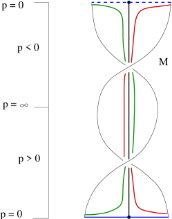
   Fig. 10: One saddle point in the surface $M$

   

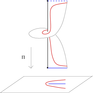
   Fig. 11: Projection of a saddle point

2. Case $n\geq 3$. The differential form (21) becomes, after dividing it by $(n-1)a_{n-1}$, into

   $$\Psi:= \Big{(}-a_{n-1}^{2}\omega+\cdots\Big{)}dv^{2}+\Big{(}na_{n-1}^{2}v+(n-2)a_{n-1}b_{n-1}\omega+\cdots\Big{)}dvd\omega\qquad$$

   $$+\Big{(}na_{n-1}b_{n-1}v+(n-1)b_{n-1}^{2}\omega+\cdots\Big{)}d\omega^{2}.$$ (27)

   Since the quadratic part of the discriminant of $\Psi$ is $n^{2}a_{n-1}^{2}(a_{n-1}v+b_{n-1}w)^{2}$, the origin is not a Morse singularity of $\Delta_{\Psi}$. Thus, we can not proceed as in the previous case.

   As a first step, consider the change of coordinates on the $v\omega$-plane

   $$\begin{pmatrix}v\\ \omega\end{pmatrix}=\begin{pmatrix}1&-\frac{b_{n-1}}{a_{n-1}}\\ 0&1\end{pmatrix}\begin{pmatrix}X\\ Y\end{pmatrix}.$$

   The differential form $\Psi$ of (ii) is transformed into the differential form

   $$\widetilde{\Omega}=\widetilde{A}(X,Y)dX^{2}+\widetilde{B}(X,Y)dXdY+\widetilde{C}(X,Y)dY^{2},$$

   where

   $$\widetilde{A}(X,Y) =a\left(X-\frac{b_{n-1}}{a_{n-1}}Y,Y\right)=Y(-a_{n-1}^{2}+\cdots),$$

   $$\widetilde{B}(X,Y) =\Big{(}b-2\frac{b_{n-1}}{a_{n-1}}a\Big{)}\left(X-\frac{b_{n-1}}{a_{n-1}}Y,Y\right)=na_{n-1}^{2}X+\cdots,$$

   $$\widetilde{C}(X,Y) =\left(\frac{b_{n-1}^{2}}{a_{n-1}^{2}}a-\frac{b_{n-1}}{a_{n-1}}b+c\right)\left(X-\frac{b_{n-1}}{a_{n-1}}Y,Y\right)=\cdots,$$

   and $a,b,c$ are the first, second and third coefficients of (ii). In what follows we consider the differential form $\Omega$ obtained of dividing $\widetilde{\Omega}$ by $a_{n-1}^{2}$, that is,

   $$\Omega:=A(X,Y)dX^{2}+B(X,Y)dXdY+C(X,Y)dY^{2},$$ (28)

   $A(X,Y)=-Y+\displaystyle\sum_{i+j=2}^{3n-3}a_{ij}X^{i}Y^{j},\ B(X,Y)=nX+\sum_{i+j=2}^{3n-3}b_{ij}X^{i}Y^{j},\ C(X,Y)=\sum_{i+j=2}^{3n-3}c_{ij}X^{i}Y^{j}$.

   As some terms of the previous coefficients depend on the degree $n$ we split the following analysis into two cases.

   1. Case $n=3$. Consider the function $G_{\Omega}:\mathbb{R}^{2}\rightarrow\mathbb{R}^{3}$ that associates to each pair $(X,Y)\in\mathbb{R}^{2}$ the coefficients $\,(C(X,Y),\,B(X,Y),\,A(X,Y))\,$ of the differential form $\Omega$. The Jacobian matrix D$G_{\Omega}$ of the map $G_{\Omega}$ at the origin is $\begin{pmatrix}0&0\\ 3&0\\ 0&-1\end{pmatrix}.$

      Since the rank of D$G_{\Omega}$ at the origin is 2, the origin is called a semi-simple singular point of $\Omega$ according to the notation of [11]. Moreover, $\Omega$ has the type of $E(\lambda)$ for $\lambda=3$. By Remark 10.1 and Lemma 9.1 of [11], the origin is a singular point of $\Omega$ with topological type of a Monstar.

   2. Case $n\geq 4$. As a second step, we will now transform the form (28) into a suitable differential form through the Blowing up method. On the $VW$-plane consider the isomorphism

      $$\phi:\mathbb{R}^{2}\setminus\{V=0\}\rightarrow\mathbb{R}^{2}\setminus\{X=0\}\mbox{ defined as }\phi(V,W)=(V,VW)=(X,Y),$$

      that is, $V=X,W=Y/X$. The pullback $\phi^{*}\Omega$ of $\Omega$ is the differential form

      $$\phi^{*}\Omega=AdV^{2}+BdVdW+CdW^{2}$$ (29)

      where $a,b,c$ denote respectively the first, second and third coefficients of $\Omega$, and

      $$A(V,W) =W^{2}c(V,VW)+Wb(V,VW)+a(V,VW),$$

      $$B(V,W) =Vb(V,VW)+2VWc(V,VW),$$

      $$C(V,W) =V^{2}c(V,VW).$$

      Since $V$ is a factor of $a,b,c$, rewrite the form $\phi^{*}\Omega$ as $\phi^{*}\Omega=V\Omega_{1}$ where

      $$\Omega_{1}:=A_{1}\ dV^{2}+VB_{1}\ dVdW+V^{2}C_{1}\ dW^{2},$$

      and $A_{1},B_{1},C_{1}$ are polynomials in $\mathbb{R}[V,W]$. A straightforward calculation shows that

      $$A_{1}(V,W)=(n-1)W+VWg_{1},\quad B_{1}(V,W)=n+Vg_{2},\quad C_{1}(V,W)=Vg_{3},$$ (30)

      where $g_{i},\,i\in\{1,2,3\}$ is a polynomial in $\mathbb{R}[V,W]$. Note that the origin is the only singular point of the form $\Omega_{1}$ on the line $V=0$.

      In a neighborhood of the origin on the $VW$-plane the two fields of directions defined by $\Omega_{1}$ are described by

      $$\Big{(}-2A_{1}\Big{)}\,dV+\Big{(}-VB_{1}+(-1)^{k}\sqrt{V^{2}(B_{1}^{2}-4A_{1}C_{1})}\Big{)}dW=0,\quad k\in\{1,2\}.$$

      Let’s denote by ${\cal F}_{k}(\Omega_{1}),k\in\{1,2\}$ the foliations corresponding to these direction fields. Consider now the vector fields

      $$Y_{k}(V,W):=(V\,T_{k},2A_{1}),\quad\mbox{with}\quad T_{k}=-B_{1}+(-1)^{k}\sqrt{B_{1}^{2}-4A_{1}C_{1}}.$$

      In a punctured neighborhood of the origin the foliation ${\cal F}_{1}(\Omega_{1})$ is tangent to the vector field $Y_{1}$ if $V>0$, and tangent to the vector field $Y_{2}$ if $V<0$. Analogously, the foliation ${\cal F}_{2}(\Omega_{1})$ is tangent to $Y_{2}$ when $V>0$, and tangent to $Y_{1}$ for $V<0$.

      From expressions (30) we infer that $T_{1}(0,0)=-2n,\$ $T_{2}(0,0)=0$ and the linear part of $Y_{1}$ at the origin is

      $$DY_{1}|_{(0,0)} = \left.\left(\begin{array}[]{cc}V\frac{\partial}{\partial V}T_{1}+T_{1}&V\frac{\partial}{\partial W}T_{1}\\ 2\frac{\partial}{\partial V}A_{1}&2\frac{\partial}{\partial W}A_{1}\end{array}\right)\right|_{\left(0,0\right)}=\left(\begin{array}[]{cc}-2n&0\\ 0&n-1\end{array}\right).$$

      Therefore, the origin is a saddle point of the field $Y_{1}$ and the eigenspaces of $DY_{1}|_{(0,0)}$ are the coordinate axes.

      On the other hand, consider the vector field

      $$\ Z_{1}(V,W)=(2VC_{1}(V,W),\ T_{1}(V,W)).$$

      Since $T_{1}(0,0)\neq 0$, the origin is a nonsingular point of this field. Moreover, because of the equality $T_{1}(V,W)\,T_{2}(V,W)=4A_{1}(V,W)\,C_{1}(V,W)$, the field $Z_{1}$ satisfies the relation

      $$2A_{1}(V,W)\,Z_{1}(V,W)=T_{1}(V,W)\,Y_{2}(V,W),$$

      which proves that $Z_{1}$ is tangent to the foliation of $Y_{2}$ (Fig. 12).

      

      Fig. 12: Foliation ${\cal F}_{1}(\Omega_{1})$

      
      

      In order to carry out a complete analysis of the singularity we will do another bluwing up of $\Omega$ as a third step.

      Consider the map $\varphi(V,W)=(VW^{2},W)=(X,Y)$. The pullback $\varphi^{*}\Omega$ of the form $\Omega$ is

      $$\varphi^{*}\Omega=(W^{4}A)\ dV^{2}+W^{2}(B+4VWA)\ dVdW+(4V^{2}W^{2}A+2VWB+C)\ dW^{2}.$$

      A straightforward calculation shows that $\varphi^{*}\Omega=W^{3}\,\Omega_{2}$ where

      $$\Omega_{2}=W^{2}A_{2}\ dV^{2}+WB_{2}\ dVdW+C_{2}\ dW^{2},$$ (32)

      where $\quad A_{2}(V,W)=-1+Wh_{1},$  $B_{2}(V,W)=b_{02}+(n-4)V+Wh_{2},$

      $C_{2}(V,W)=c_{03}+(c_{11}+2b_{02})V+(2n-4)V^{2}+Wh_{3},\,\$ and

      $h_{k},\$ is a polynomial in $\mathbb{R}[V,W]\$ for $\ k\in\{1,2,3\}$.

      The two fields of directions defined by $\Omega_{2}$ are described, in a neighborhood of the origin on the $VW$-plane by

      $$\Big{(}-WB_{2}+(-1)^{k}\sqrt{W^{2}(B_{2}^{2}-4A_{2}C_{2})}\Big{)}\,dV+\Big{(}-2C_{2}\Big{)}dW=0,\quad k\in\{1,2\}.$$

      Let’s denote by ${\cal F}_{k}(\Omega_{2}),\,k\in\{1,2\}$ the foliations of these fields. Consider the vector fields

      $$Y_{k}(V,W):=(2C_{2},\,W\,T_{k}),\quad\mbox{with}\quad T_{k}=-B_{2}+(-1)^{k}\sqrt{B_{2}^{2}-4A_{2}C_{2}}.$$

      In a punctured neighborhood of the origin the foliation ${\cal F}_{1}(\Omega_{2})$ is tangent to the vector field $Y_{1}\,$ if $\,W>0$, and tangent to the vector field $Y_{2}\,$ if $\,W<0$. Analogously, the foliation ${\cal F}_{2}(\Omega_{2})$ is tangent to $Y_{2}$ when $W>0$, and tangent to $Y_{1}$ for $W<0$.

      On the other hand, in the following analysis we will also consider the vector fields

      $$\ Z_{k}(V,W)=(2\,V\,C_{2}(V,W),\ T_{k}(V,W))\ \mbox{ for }k\in\{1,2\}.$$

      Because of the equality $T_{1}(V,W)\,T_{2}(V,W)=4A_{2}(V,W)\,C_{2}(V,W)$, the field $Z_{k},\ k\in\{1,2\}$ satisfies the relation

      $$2\,C_{2}(V,W)\,Z_{k}(V,W)=T_{k}(V,W)\,Y_{3-k}(V,W).$$ (33)

      In what follows we will need the following coefficients:

      $$b_{02}=\frac{(n-2)(n-3)K}{(n-1)a_{n-1}^{3}},\quad c_{11}=\frac{2n(n-2)K}{(n-1)a_{n-1}^{3}},\quad c_{03}=\frac{2(n-2)^{2}K^{2}}{(n-1)a_{n-1}^{6}},\quad$$ (34)

      where $K:=a_{n-2}b_{n-1}^{2}+a_{n-1}^{2}r_{n-2}-a_{n-1}b_{n-1}b_{n-2}\$ and $\ f_{n-2}(u,v)=\displaystyle\sum_{\begin{subarray}{c}i=0\end{subarray}}^{n-2}r_{i}\,u^{i}v^{n-1-i}.$

      The singular points of $\Omega_{2}$ on the line $W=0$ are given by the equation $\ C_{2}(V,0)=0,$ that is, $\ c_{03}+(c_{11}+2b_{02})V+(2n-4)V^{2}$. The discriminant of this cuadratic equation is $\Delta=\frac{4(n-2)^{2}K^{2}}{(n-1)^{2}a_{n-1}^{6}}$ which is positive if and only if $K\neq 0$. Therefore, the singular points on $W=0$ are

      $$p_{j}:=\left(-\frac{(2n-3)K\ }{2(n-1)a_{n-1}^{3}}(-1)^{j}\sqrt{\frac{K^{2}}{4(n-1)^{2}a_{n-1}^{6}}}\,,\ 0\right),\ \mbox{ for }j\in\{1,2\}.$$

      Suppose $K/a_{n-1}>0$. This condition implies that $\,V_{1}=-\frac{K}{a_{n-1}^{3}},\ V_{2}=-\frac{(n-2)K}{(n-1)a_{n-1}^{3}}\,$ and both roots are negative. From expressions (34) we derive that $\ T_{1}(p_{1})=-\frac{4K}{(n-1)a_{n-1}^{3}},$ $\,T_{1}(p_{2})=-\frac{2(n-2)K}{(n-1)a_{n-1}^{3}}\$ and the linear part of $Y_{1}$ at $p_{j}$ is

      $$DY_{1}|_{P_{j}}=\left\{\begin{aligned} &\left(\begin{array}[]{cc}-\frac{4(n-2)K}{(n-1)a_{n-1}^{3}}&2\frac{\partial C_{2}}{\partial W}(p_{1})\\ 0&-\frac{4K}{(n-1)a_{n-1}^{3}}\end{array}\right)\ \mbox{ for }j=1,\\ &\left(\begin{array}[]{cc}\frac{4(n-2)K}{(n-1)a_{n-1}^{3}}&\ \ 2\frac{\partial C_{2}}{\partial W}(p_{1})\\ 0&\ \ -\frac{2(n-2)K}{(n-1)a_{n-1}^{3}}\end{array}\right)\ \mbox{ for }j=2.\end{aligned}\right.$$

      Therefore, $p_{1}$ is a node point of the field $Y_{1}$, and $p_{2}$ is a saddle point. On the other hand, since $T_{1}(p_{j})\neq 0\$ for $j\in\{1,2\}$, the point $p_{j}$ is a nonsingular point of $Z_{1}$. Moreover, according to (33) the field $Z_{1}$ is tangent to the foliation of $Y_{2}$. We remark that analogous results are obtained when $K/a_{n-1}<0$.

      From all the previous analysis we conclude that the the origin on the $v\omega$-plane has the topological type of a Monstar when $K\neq 0$. This completes the proof of Theorem 4.5. $\Box$

Acknowledgments The second author thanks to the PASPA-DGAPA, UNAM Program for its finantial support during the preparation of this work and also thanks to the Institute of Technology, Tralee for its hospitality.

References

- [1] N. Ando, The behavior of the principal distributions on the graph of a homogeneous polynomial, Tohoku Math. J. 54 (2002) 163-177.
- [2] J. W. Bruce, D. L. Fidal, On binary differential equations and umbilics, Proc. R. Soc. Edinburgh 111A (1989) 147-168.
- [3] J. W. Bruce, F. Tari, On binary differential equations, Nonlinearity 8 (1995) 255-271.
- [4] A. Cayley, On differential equations and umbilici, In The Collected Mathematical Papers (Cambridge Library Collection - Mathematics), Cambridge: Cambridge University Press (2009) 115-130.
- [5] G. Darboux, Sur la forme des lignes de courbure dans le voisinage d’un ombilic, Leçons sur la théorie des surfaces, vol. IV Note 07, Gauthier Villars, Paris, 1896.
- [6] R. Garcia, J. Sotomayor, Lines of curvature on algebraic surfaces, Bull. Sci. math. 120 (1996) 367-395.
- [7] R. Garcia, J. Sotomayor, Lines of principal curvature near singular end points of surfaces in , Adv. Studies in Pure Mathematics 43 (2006) 437-462.
- [8] M. A. Guadarrama-García, Master dissertation, U.N.A.M., 2012.
- [9] M. A. Guadarrama-García, A. Ortiz-Rodríguez, On the geometric structure of certain real algebraic surfaces, Geom Dedicata 191 No.1 (2017) 153-169.
- [10] V. Guíñez, Nonorientable Polynomial Foliations on the Plane, J. Differ. Equations 87 (1990) 391-411.
- [11] V. Guíñez, Locally Stable Singularities for Positive Quadratic Differential Forms, J. Differ. Equations 110 (1994) 1-37.
- [12] C. Gutierrez, V. Guíñez, Positive quadratic differential forms : linearization, finite determinacy and versal unfolding, Ann. Fac. Sci. Toulouse: Math., Sér. 6 Vol. 5 No. 4 (1996) 661-690
- [13] C. Gutierrez, J. Sotomayor, Structurally stable configurations of lines of principal curvature, Astérisque, Tome 98-99 (1982) 195-215.
- [14] J. P. S. Kung, G-C. Rota, The theory of binary forms, Bull. Amer. Math. Soc. 10 (1984) 27-85.
- [15] G. Monge, Sur les lignes de courbure de la surface de l’ellipsoïde, Journ. de l’Ecole Polytechnique, Math. (1795) 145-165.
- [16] P. J. Olver, Classical invariant theory and the equivalence problem for particle Lagrangians. I. Binary forms, Adv. in Math. 80 No. 1 (1990) 39-77.
- [17] H. Poincaré, Mémoire sur les courbes définies par une équation différentielle. J. Math. Pure Appl. 7 (1881) 375-422.
- [18] T. A. Springer, Invariant Theory, Lecture Notes in Math. 585 Springer-Verlag, New York, 1977.
- [19] V. A. Toponogov, On conditions for existence of umbilical points on a convex surface, Siberian Math. J. 36 No. 4 (1995) 780-786.