The Minimum Energy Principle Applied to Parker’s Coronal Braiding and Nanoflaring Scenario

Abstract

Parker’s coronal braiding and nanoflaring scenario predicts the development of tangential discontinuities and highly misaligned magnetic field lines, as a consequence of random buffeting of their footpoints due to the action of sub-photospheric convection. The increased stressing of magnetic field lines is thought to become unstable above some critical misalignment angle and to result into local magnetic reconnection events, which is generally referred to as Parker’s “nanoflaring scenario”. In this study we show that the minimum (magnetic) energy principle leads to a bifurcation of force-free field solutions for helical twist angles at $|\varphi(t)|=\pi$, which prevents the build-up of arbitrary large free energies and misalignment angles. The minimum energy principle predicts that neighbored magnetic field lines are almost parallel (with misalignment angles of $\Delta\mu\approx 1.6^{\circ}-1.8^{\circ}$), and do not reach a critical misalignment angle prone to nanoflaring. Consequently, no nanoflares are expected in the divergence-free and force-free parts of the solar corona, while they are more likely to occur in the chromosphere and transition region.

1 INTRODUCTION

The sub-photospheric layers of the Sun exhibit vigorous convective motions, which are driven by a negative vertical temperature gradient $dT/dh<0$ due to the Bénard-Rayleigh instability (Lorenz 1963). The convective motion of the sub-photospheric fluid is a self-organizing process that creates granules with a characteristic size $\ell\approx 1000$ km and horizontal velocity $v\approx 2$ $\rm km~{}s^{-1}$. It follows that the convective motions have a typical time scale $\tau=\ell/v\approx 500$ s, or 7 minutes, which matches the observed life time of granules. The question now arises how the solar photosphere affects the coronal magnetic field. In Parker’s theory for solar coronal heating (Parker 1972, 1983), a coronal loop is perturbed by small-scale, random motions of the photospheric footpoints of the coronal field lines, driven by sub-photospheric convective flows. According to Parker, these motions lead to twisting and braiding of the coronal field lines. As the magnetic field evolves, thin current sheets are formed in the corona, and energy is dissipated by magnetic reconnection. The reconnection is likely to occur in a burst-like manner as a series of “nanoflares” (Parker 1988). Parker’s magnetic braiding scenario has become the main paradigm for coronal heating in active regions, and the nanoflare heating theory has been widely adopted (see reviews by Cargill 2015; Klimchuk 2015; Aschwanden 2005). However, the response of the coronal magnetic field to random footpoint motions is a complex physical problem, and the implications of Parker’s theory are not yet fully understood.

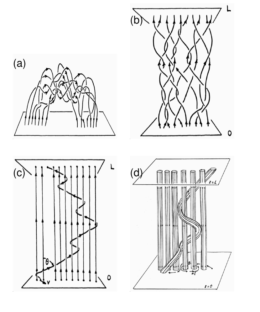
Figure 1: Original cartoons published by Eugene Parker (1989): Schematic drawings of field lines of a bipolar magnetic reconnection region above the photosphere (a); a bundle of loops stretched out in vertical direction (b); a wandering (braiding) field line among neighboring field lines (c), and a single flux tube after some random walk of its footpoint (d).

Parker (1983, 1988) created several cartoons that depict how the random motion of coronal magnetic field lines (or lines of force) wind around neighbored, less-twisted (or untwisted) field lines (Fig. 1), either for dipolar field lines (Fig. 1a) or in the form of stretched-out flux tubes (Fig. 1b). The winding motion has been aptly called “coronal loop braiding,” although it has never been demonstrated that a braided field can be formed by random motions of the photospheric footpoints. Some cartoons display a single braided field line among a set of untwisted (straight) field lines (Fig. 1c), or a single flux tube surrounded by a set of untwisted (straight) flux tubes (Fig. 1d). The magnetic braiding model predicts that the misalignment angle between a braided field line and a neighboring less-braided field line will increase with time, building up magnetic stress until a reconnection event is triggered, which causes some or all of the magnetic energy to be released.

When a coronal loop system is viewed from the side, it generally shows a collection of nearly parallel threads that do not cross each other, and neighboring threads are co-aligned to within a few degrees. The threads are believed to follow the magnetic field ${\bf B}({\bf r})$, so the direction of ${\bf B}$ in neighboring threads must be co-aligned to within a few degrees. In many cases the average direction of the threads is consistent with that predicted by potential field models. Therefore, the observations provide little evidence for the presence of braided fields with misalignment angles of about 20 degrees relative to the potential field, as predicted by Parker (1983). The observations are consistent with the much simpler geometries rendered in Figure 2, which shows a dipolar flux tube system with slightly twisted (Fig. 2a,b) or a strongly twisted (Fig. 2c,d) flux tubes.

In this paper we consider the assumptions of Parker’s braiding model and its suitability to explain the observed coronal loops. We argue that the model is not internally consistent because it predicts that thin current sheets will form quickly, but reconnection is assumed to be postponed until the braided field is fully formed. It is not clear that a braided field will form because the timescale for the formation of thin current sheets (a few minutes) is much shorter than the time needed to build up the braided field (hours). We propose an alternative “solution” to the Parker problem in which reconnection causes the magnetic field to remain close to a minimum energy state in which the field lines do not deviate strongly from straight lines (also see Rappazzo & Parker 2013; Rappazzo 2015). According to this scenario, the relative displacements of the footpoint at the two boundary plates in the Parker model are not much larger than the correlation length $\ell$ of the footpoint motions. We also compare the predictions of the minimum energy scenario with results from MHD simulations, and discuss the role of magnetic braiding in coronal heating. We find that quasi-static braiding driven by granule-scale footpoint motions cannot provide enough energy to heat active-region loops to the observed temperatures and densities.

2 RECONNECTION IN THE MAGNETIC BRAIDING MODEL

Parker (1972, 1983) considered a simplified model for a coronal loop in which an initially uniform field is contained between two parallel plates, which represent the photosphere at the two ends of the loop. The coronal plasma is assumed to be highly conducting, so the magnetic field is nearly “frozen” into the plasma. The loop is anchored in the photosphere at its two ends, and its length $L$ is assumed to be much larger than its width, so the curvature of the loop can be neglected. A cartesian coordinate system $(x,y,z)$ is used with the $z$-axis along the (straigthened) loop. The planes $z=0$ and $z=L$ represent the photosphere at the two ends of the loop, and the “corona” is the region in between these planes ($0<z<L$). At time $t=0$ the magnetic field is assumed to be a uniform potential field, ${\bf B}({\bf r},0)=B_{0}\hat{\bf z}$, where $B_{0}$ is the field strength. The field is perturbed by random footpoint motions at $z=0$ and $z=L$, which cause random twisting and braiding of the coronal field lines. In this model all details of the lower atmosphere are neglected, and footpoint motions with velocities of 1 – 2 $\rm km~{}s^{-1}$ are applied directly at the coronal base. This simplified version is very useful because it is well defined mathematically and can be studied in great detail.

In the Parker problem the footpoint velocities are assumed to be incompressible ($\nabla_{\perp}\cdot{\bf v}_{\perp}=0$), and vary randomly in space and time. The auto-correlation time $\tau$ is assumed to be large compared to the Alfvén travel time $L/v_{A}$ in the corona. Then the coronal field will remain close to a force-free state in which the Lorentz force nearly vanishes, ${\bf j}\times{\bf B}\approx 0$, where ${\bf j}({\bf r},t)$ is the electric current density (quasi-static braiding). The magnetic stresses will build up over time, and in some locations the stress will become so large that some energy is released by small-scale reconnection. Hence, we expect that the magnetic field will evolve quasi-statically most of the time, but this evolution will sometimes be interrupted by reconnection events where magnetic free energy is converted into heat of the plasma.

Parker (1983) argued on the basis of the observed coronal heating rates that, starting from an initial uniform field, the photospheric footpoints motions must continue for a period of about 8 hours before reconnection can start removing some of the energy. This long energy buildup time is needed because the transverse component of the coronal field must build up to a significant fraction of the parallel component, otherwise the rate of energy input into the corona (the Poynting flux at the coronal base) is too low compared to the plasma heating rate. During this buildup phase strong electric currents develop in between the mis-aligned coronal flux tubes.

In the following we argue that the concept of magnetic braiding, although convincing in cartoon representations (Fig. 1), may not be the correct solution to the Parker problem. On the one hand, the braiding model predicts the “spontaneous formation of tangential discontinuities” in the magnetic field, i.e., the formation of thin current sheets (Parker 1972). Although the validity of Parker’s (1972) argument has been questioned (e.g., van Ballegooijen 1985), it is expected that thin current sheets will develop in the Parker problem on the timescale of the solar granulation (at most a few minutes). This is certainly the case when discrete flux tubes are shuffled about as indicated in Fig. 1d. On the other hand, the model assumes that magnetic reconnection somehow does not occur at these current sheets until the braided field is fully formed. This is unlikely because the corona has a small but finite resistivity, and thin current sheets are expected to be unstable to resistive instabilities such as tearing modes (e.g., Tenerani et al. 2016). Therefore, thin current sheets cannot exist for the time needed to build up the braided field, which requires about 8 hours (Parker 1983). Hence, the magnetic braiding model is not internally consistent: it assumes magnetic reconnection is somehow prevented until the braided field has fully formed, then reconnection is “turned on” to explain the release of energy in nanoflares. Instead, one would expect that reconnection occurs whenever thin current sheets are present. Magnetic energy will then be released well before the braided field is fully formed.

Other analytical studies predicted a somewhat different scenario for what happens in the Parker problem. Van Ballegooijen (1985) proposed that the random footpoint motions cause a “cascade” of magnetic energy towards smaller spatial scales, even though the field evolves through a series of force-free states and the plasma is not turbulent in the traditional sense. This cascade model predicts the formation of thin current layers on a time scale of a few times the dynamical time of the footpoint motions (a few minutes). This is larger than the time for the “spontaneous formation of tangential discontinuities” (Parker 1972), which presumably occurs on the Alfvén time scale ($L/v_{A}\sim 30$ s), but is much shorter than the 8-hour period needed to form a braided field of sufficient complexity (Parker 1983). Strongly braided fields do not develop in the cascade model, and the predicted dissipation rates are a factor 10 to 40 lower than the observational requirements (van Ballegooijen 1986). Therefore, the cascade model fails as a theory for coronal heating, but it may give a more accurate description of what happens in the Parker problem when reconnection is allowed to occur.

3 THE MINIMUM ENERGY SCENARIO

The above considerations lead us to propose a somewhat different solution of the Parker problem in which magnetic reconnection is assumed to occur so frequently that the magnetic field lines never deviate very far from straight lines connecting the photospheric footpoints. The concept is first illustrated using a helically twisted cylindrical flux tube, then is generalized for random footpoint motions.

3.1 Helically Twisted Magnetic Fields

We use a parameterization of the 3-D magnetic field in terms of helically twisted cylindrical flux tubes, for which analytical divergence-free and force-free solutions of the magnetic field are known, either for a straight cylinder (Priest 1982), or in form of the vertical-current approximation nonlinear force-free field (VCA-NLFFF) model (Appendix A), which accommodates the full 3-D geometry of the spherical solar surface and the curvature of loops, being accurate to second order of $\alpha$ (Aschwanden 2013a).

We consider two magnetic field lines, one being a braiding field line (solid linestyle in Fig. 3 top), and the other one a less-braided (straight) field line (dashed linestyle in Fig. 3 top). The random footpoint motion at $L=0$ is represented, without loss of generality, by a circular motion at the photospheric level (z=0). The footpoint rotation moves the footpoint position from its initial location at $(x_{1},y_{1},z_{1}=0)$ (Fig. 3a) to rotation angles of $\varphi=\pi/2$ (Fig. 3b), $\varphi=\pi$ (Fig. 3c), $\varphi=\pi(3/2)$ (Fig. 3d), and finally back to the identical position where we started $(x_{1},y_{1},z_{1}=0)$ (Fig. 3e). The geometry of the twisted field line (solid curve in Fig. 3 top) results into a helix rotated by one full turn, which corresponds to a divergence-free and force-free solution in cylindrical or spherical coordinates (Appendix A, Eqs. A3-A6). We can define the angle between the twisted field line (at radius $r$) and an untwisted field line (at the cylindrical symmetry axis) with a misalignment angle $\mu$ (Fig. 4),

$$\tan{(\mu)}={\left({B_{\varphi}\over B_{p}}\right)}={\left({\varphi r\over L}\right)}\ ,$$ (1)

where $r$ is the radial distance from the loop symmetry axis, $L$ is the loop length, and $\varphi$ is the rotation angle of the twisted flux tube. The rotation angle $\varphi$ is simply defined by the number $N_{turn}$ of turns,

$$\varphi=2\pi N_{turn}\ .$$ (2)

The free energy density $\varepsilon_{free}=\varepsilon_{\varphi}$, which is the difference between the non-potential $\varepsilon_{np}=B_{np}^{2}/8\pi$ and the potential energy $\varepsilon_{p}=B_{p}^{2}/8\pi$, where $B_{np}$ is the nonpotential field, and $B_{p}$ is the potential field (Aschwanden 2013b),

$$\varepsilon_{free}=(\varepsilon_{np}-\varepsilon_{p})=\varepsilon_{\varphi}={B_{\varphi}^{2}\over 8\pi}\ ,$$ (3)

can be expressed with Eqs. (1) and (3) as a function of the rotation angle $\varphi$, which shows that the free energy density is zero for no twist or for a potential field, but is monotonically increasing with the square of the rotation angle $\varphi$ (using Eqs. 1 and 3),

$$\varepsilon_{free}={1\over 8\pi}\left({B_{p}\varphi\ r\over L}\right)^{2}\ ,$$ (4)

The twisted helical field line shown in Fig. 3 clearly illustrates the dynamics of Parker’s braiding model. If we continue to twist the helical cylinder, say by one full turn, the resulting helical loop will have a full turn, which we can continue until we obtain a “slinky” with an arbitrary large number of turns, and hence, arbitrary large free energy. The free energy density increases quadratically with the rotation angle, $\varepsilon_{free}\propto\varphi^{2}$ (Eq. 4). Mathematically, there is no upper limit on the number of twist and on the free energy density, which illustrates Parker’s dilemma that braiding leads to infinite energies, if it is not reduced by occasional magnetic reconnection episodes, or by nanoflare events above some critical threshold of the rotation (or twist) angle $\varphi$.

Let us now consider a slightly different model that we call the minimum energy model for short, referring to the minimum of the free magnetic energy density. We start with the same configuration of two parallel field lines (Fig. 3f), of which one is increasingly twisted by a rotating footpoint motion (Fig. 3g). For a small twist angle (say $\varphi=\pi/2$) the twisted field line has the same force-free solution (Fig. 3g) as in Parker’s braiding model (Fig. 3b). This is the case until we reach a twist angle of a half turn ($\varphi=\pi$) (Figs. 3c and Fig. 3h), at which point we encounter a bifurcation in the path of possible force-free magnetic field solutions. In Parker’s scenario, the number of helical turns increases, while the number of helical turns decreases in the minimum energy model, until it reaches the potential field solution of no twist after a rotation angle of one full turn ($\varphi=2\pi$) (Fig. 3j). The different behavior results from the ambiguous path after the bifurcation at $\varphi(t)=\pi$. The twisting process has two options, either to increase the rotation angle, or to decrease the rotation angle. The minimum energy principle requires the path of lower free energy density, because the lower energy state has a higher statistical probability than the higher energy state. Thus, the minimum energy principle sets an upper limit for the rotation angle,

$$|\varphi|\leq\pi\ .$$ (5)

The resulting dependence of the free energy density $\varepsilon_{\varphi}(\varphi)$ is shown in Fig. 5, for Parker’s braiding scenario (with quadratically increasing free energy as a function of time), while the minimum energy scenario follows a decreasing free energy density after passing the maximum rotation angle limit $\varphi(t)=\pi$ at the bifurcation point.

We can generalize our argument of the circular motion of a helically twisted field line to random walk motion of braided field lines. We simulate a random walk of the rotation angle $\varphi(t)$ that follows a diffusive pattern $\varphi(t)\propto t^{1/2}$ (Fig. 6, solid curve) for Parker’s braiding scenario. For the minimum energy scenario, however, a bifurcation sets in at $|\varphi|\leq\pi$ and the path evolves along smaller rotation angles (Fig. 6, dashed curve), preventing divergence to large free energies, large rotation angles $\varphi(t)$, or large misalignment angles $\mu(t)$, according to Eq. (1).

3.2 Random Footpoint Motions

We now generalize the above argument to random walk of the photospheric footpoints analytically. A magnetic flux bundle with a square cross-section of width $w$ is considered. The magnetic perturbations can be described in terms of the shapes of the field lines. These shapes are given by functions $X(x_{0},y_{0},z,t)$ and $Y(x_{0},y_{0},z,t)$, where $x_{0}$ and $y_{0}$ are labels of the field lines. Each field line is given by a curve with cartesian coordinates $[X(x_{0},y_{0},z,t),Y(x_{0},y_{0},z,t),z]$, where $z$ parameterizes the curve. The three components of the magnetic field are

$$B_{x}=\frac{B_{0}}{J}\frac{\partial X}{\partial z},~{}~{}~{}~{}~{}B_{y}=\frac{B_{0}}{J}\frac{\partial Y}{\partial z},~{}~{}~{}~{}~{}B_{z}=\frac{B_{0}}{J},$$ (6)

where $B_{0}$ is the strength of the original uniform field, and $J$ is the Jacobian on the mapping from $(x_{0},y_{0})$ to $(X,Y)$:

$$J(x_{0},y_{0},z,t)\equiv\frac{\partial X}{\partial x_{0}}\frac{\partial Y}{\partial y_{0}}-\frac{\partial Y}{\partial x_{0}}\frac{\partial X}{\partial y_{0}}.$$ (7)

We assume the loop is much longer than its width ($L\gg w$), so that the parallel components of the field is nearly constant, $J=1$. During the time interval before onset of reconnection ($0<t<t_{R}$), the coordinates $(x_{0},y_{0})$ are given by the initial positions of the field lines, but later on some field lines will have reconnected and $(x_{0},y_{0})$ are no longer given by the initial coordinates. The energy of the system is given by a volume integral of the magnetic free energy density:

$$E(t)=\frac{B_{0}^{2}}{8\pi}\int_{0}^{L}\int_{0}^{w}\int_{0}^{w}\left[\left(\frac{\partial X}{\partial z}\right)^{2}+\left(\frac{\partial Y}{\partial z}\right)^{2}\right]dx_{0}dy_{0}dz.$$ (8)

The boundary conditions for $X$ and $Y$ are the positions of the field lines at the boundary plates. A lower bound on the energy can be obtained by assuming that the field lines are nearly straight lines connecting the footpoints at $z=0$ and $z=L$:

$$\frac{\partial X}{\partial z}\approx\frac{\Delta X}{L},~{}~{}~{}~{}~{}~{}~{}\frac{\partial Y}{\partial z}\approx\frac{\Delta Y}{L},$$ (9)

where $\Delta X$ and $\Delta Y$ are relative displacements of the footpoints:

$$\Delta X(x_{0},y_{0},t) \equiv X(x_{0},y_{0},L,t)-X(x_{0},y_{0},0,t),$$ (10)

$$\Delta Y(x_{0},y_{0},t) \equiv Y(x_{0},y_{0},L,t)-Y(x_{0},y_{0},0,t).$$ (11)

Then the minimum energy is

$$E_{\rm min}(t)=\frac{B_{0}^{2}}{8\pi L}\int_{0}^{w}\int_{0}^{w}\left[(\Delta X)^{2}+(\Delta Y)^{2}\right]dx_{0}dy_{0}.$$ (12)

When the displacements $\Delta X$ and $\Delta Y$ become much larger than the correlation length $\ell$ of the footpoint motions, the field lines are forced to bend around each other, causing the formation of thin current sheets where reconnection can take place. The newly reconnected field lines will tend to be more straight and have smaller footpoint displacements, causing the magnetic stress to be reduced. Therefore, we expect that the footpoint displacements remain limited in magnitude,

$$|\Delta X|\sim|\Delta Y|\sim\ell,$$ (13)

and the minimum energy will saturates at a value given by

$$E_{\rm min}\sim\frac{B_{0}^{2}w^{2}\ell^{2}}{4\pi L}.$$ (14)

Note that this expression (Eq. 14) of the free energy calculated based on random motion of the footpoints is equivalent to the free energy density $\varepsilon_{free}$ defined for a helically twisted loop (Eq. 4), if we define the 2-D correlation length with $\ell=\sqrt{2}r\varphi$ and execute the volume integral $E_{\rm min}=\varepsilon_{free}\ V$ of the free energy density $\varepsilon_{free}$ with the volume definition $V=w^{2}L$, based on the width $w$ and length $L$ of a loop.

We suggest the actual free energy $E$ will not be much larger than $E_{\rm min}$. The above analysis is consistent with the work of Rappazzo & Parker (2013) and Rappazzo (2015), who argue that there is a threshold for the formation of thin current sheets, $B_{\perp}\sim B_{0}\ell/L$, which corresponds to Eq. (14). Therefore, the minimum energy scenario suggests that magnetic reconnection will prevent the build-up of arbitrary large transverse fields. The transverse displacements remain on the order of the scale of the solar granulation, $\ell\approx 1000$ km, and a strongly braided field does not form.

4 DISCUSSION

4.1 Criticism of Parker’s Braiding Scenario

The “magnetic field braiding” scenario of Parker (1988) suggests that the X-ray corona is created by the dissipation of the many tangential discontinuities arising spontaneously in the bipolar fields of the active regions of the Sun as a consequence of random continuous motion of the footpoints of the field in the photospheric convection. This concept implies that the field lines become increasingly more twisted and braided by the random motion of the footpoints, as depicted in the cartoons of Parker’s (1983) scenario (Fig. 1). Although cartoons are not intended to provide a scientific accurate model on scale, they should convey the correct concept qualitatively. However, three major criticisms can be discussed about the cartoons featured in Fig. 1: (i) the discontinuity of the magnetic field, (ii) the large misalignment angles, and (iii) the location of nanoflares.

The first criticism, i.e., the discontinuity of the magnetic field between a braided field line and a unbraided (or less-braided) field line is most conspicuously depicted in Fig. 1d. Even if both types of field lines would correspond to a physical solution of Maxwell’s or the ideal MHD equations, they cannot evolve independently of each other, as the cartoon in Fig. 1d suggests. If one field line becomes twisted, a continuous field solution (that fulfills the divergence-freeness and force-freeness) affects the adjacent field lines in such a way that only small misalignment angles between two neighbored field lines occur, as depicted in Fig. 2. In this sense, discontinuities in the 3-D magnetic field solution are unobserved and unphysical.

The second criticism, i.e., the large misalignment angles between adjacent magnetic field lines predicted by Parker’s braiding model is related to the unphysical discontinuity of the magnetic field. We can estimate the typical misalignment angle between two adjacent field lines in the following way. Two field lines with a distance $r$ and $r+\Delta r$ from the symmetry axis of a flux tube have an angle of $\mu$ and $\mu+\Delta\mu$ relative to the symmetry axis, and the misalignment angle $\Delta\mu$ between the two adjacent field lines is according to Eq. (1),

$$\Delta\mu=\arctan{\left({\varphi[r+\Delta r]\over L}\right)}-\arctan{\left({\varphi r\over L}\right)}\ ,$$ (15)

For instance, for field lines with distances of $r=0,1,2,...,10$ Mm from the flux tube axis, at a relative distance of $\Delta r=1$ Mm, a length of $L=100$ Mm, and twisted by a half turn ($\phi=\pi$), we obtain with Eq. (6) misalignment angles of $\Delta\mu\approx 1.6^{\circ}-1.8^{\circ}$. Such scales of small misalignment angles are approximately rendered in the revised cartoons shown in Fig. 2, in contrast to the large misalignment angles of order $\Delta\mu\approx 45^{\circ}$ shown in Fig. 1. Also, observations with TRACE and AIA/SDO of the corona in EUV wavelengths show invariably near-parallel loops, e.g., as determined from stereoscopic triangulation (Aschwanden et al. 2008).

The third criticism of Parker’s braiding scenario is the location of nanoflares, which would be expected throughout the corona, since uniformly twisted flux tubes have a constant twist angle (or a constant $\alpha$-parameter) along the loops. In contrast, if a divergence-free and force-free solution of magnetic fields is calculated (such as depicted in Fig. 2), misalignment angles in the force-free corona are small, and therefore no tangential discontinuities arise, and thus no nanoflares are produced in the force-free corona. However, the chromosphere and parts of the transition region are not force-free, and thus tangential discontinuities and nanoflaring are expected there. This is indicated with misalignments of the chromospheric footpoints in Fig. 2. According to measurements and modeling of the 3-D magnetic field with the virial theorem, the chromosphere was found to be not force-free up to a height of $h\approx 400$ km (Metcalf et al. 1995). Another (observational) argument for nanoflare locations in the chromosphere and transition region are EUV observations (Aschwanden et al. 2000) and hard X-ray observations of microflares (Hannah et al. 2001).

Of course, these three criticisms, (i) the discontinuity of the field, (2) the misalignment of adjacent field lines, and (iii) the location of nanoflares are all related to each other. If there is no discontinuity, then there is no misalignment, and no nanoflaring, but the three aspects can be measured from observations each separately.

4.2 Limits of the Energy Build-Up

A new aspect of this critics on Parker’s nanoflare scenario is the minimum energy aspect. Using the concept of helical twisting in the build-up of free energy we have shown that the free energy evolves in a nonlinear (quadratic) way with the twisting or rotation angle, i.e., $\varepsilon_{\varphi}\propto\varphi^{2}$, which introduces a bifurcation at $|\varphi(t)|=\pi$. Whenever such a bifurcation point is reached during the random shuffling of the footpoints of coronal loops, the lower energy state is statistically more likely to be chosen, which prevents an infinite build-up of free energy.

This is also consistent with the kink instability criterion (Török and Kliem 2003; Kliem et al. 2004), which limits the maximum stable solution to about $\lower 1.72218pt\hbox{$\;\buildrel<\over{\scriptstyle\sim}\;$}1$ helical turn (Hood and Priest 1979; Sakurai 1976; Mikic et al. 1990). If loops or filaments are helically twisted by a larger number or turns, they become unstable and erupt.

4.3 Numerical MHD Simulations

Many authors have studied magnetic braiding using 3-D MHD simulations (e.g., Mikic et al. 1989; Hendrix et al. 1996; Longcope and Sudan 1994; Ng and Bhattacharjee 2008; Galsgaard and Nordlund 1996, 1999; Rappazzo 2007, 2008; Dahlburg et al. 2016). This work has provided much insight into the structure and topology of braided fields, and the formation of current sheets in such models. However, none of these models has been able to reproduce the strongly braided fields predicted by Parker (1983). In most cases the field lines deviate only slightly from straight lines connecting the footpoints at the two boundary plates, consistent with the predictions of the minimum energy scenario.

In most cases detailed comparisons between observed and predicted coronal heating rates have not been made. Therefore, it is still an open question whether magnetic braiding models based on results from 3-D MHD simulations (as opposed to cartoons) are consistent with the observed properties of coronal loops. In order to have a valid comparison, the footpoint motions imposed in magnetic braiding models must be consistent with the observed motions of magnetic elements on the photosphere. In particular, observations of random-walk diffusion constants (see Berger 1998, and references therein) provide important constraints on the rate at which magnetic energy can be injected into coronal loops by random footpoint motions. The imposed footpoint motions should be consistent with these diffusion constants, otherwise the coronal heating rate may be overestimated.

The 3-D MHD model for a coronal loop has been extended to include an approximate description of the lower atmosphere (van Ballegooijen et al. 2011, 2014; Asgari et al. 2012, 2013, 2014, 2015). In this model Alfvén waves are launched in kilogauss flux tubes in the photosphere, and the waves travel upward into the corona, where wave dissipation and plasma heating take place. Magnetic braiding occurs in these models, but the braiding is more dynamic in nature because the Alfvén travel time from one photosphere footpoint to the other (about 2 minutes) is comparable to the timescale of the imposed footpoint motions. Therefore, when the lower atmosphere is included in the model, the corona responds much more dynamically to the footpoint motions, not quasi-statically as assumed in the Parker’s braiding model and in the cascade model (van Ballegooijen 1986). Quasi-static evolution was recovered only when the lower atmosphere was removed from the model (see section 3 in van Ballegooijen et al. 2014). This dynamic behavior for models that include the lower atmosphere is a consequence of the much higher density of these layers compared to the corona.

An observed coronal loop is expected to be rooted in multiple photospheric flux elements, and in plage regions these elements are expected to merge into a space-filling field at some height in the chromosphere. Recently, van Ballegooijen et al. (2017) simulated the dynamics of Alfvén waves in a coronal loop rooted in multiple flux tubes. They also developed a second “magnetic braiding” model in which the footpoint motions are applied in the low chromosphere, and realistic photospheric velocities and correlation times are used (see section 5 of that paper). They found that the energy injected into the corona by magnetic braiding is much less than that provided by Alfvén waves, and is insufficient to compensate for the radiative and conductive losses from the corona. The main reason for this low energy input rate is that the energy builds up only for about 20 minutes, after which the energy dissipation rate becomes equal to the energy input rate. This 20-minute build-up time is much shorter than the 8-hour period shown to be required by Parker (1983). Therefore, a strongly braided field never develops in this model.

The above result is consistent with predictions from the cascade model (van Ballegooijen 1986). According to this model, quasi-static braiding causes the thickness $\delta(t)$ of the coronal current sheets to decrease exponentially with time, $\delta(t)\sim e^{-t/\tau}$. The time scale $\tau$ is determined by the dynamical time of the footpoint motions and is only a few minutes. When $\delta(t)$ reaches the magnetic diffusion scale, reconnection will start and will soon dominate the evolution of the magnetic structure. The onset of reconnection occurs at a time $t_{R}\approx\text@frac{1}{2}\tau\ln R_{m}$, where $R_{m}$ is the magnetic Reynolds number. Even for the very high Reynolds numbers found on the Sun ($R_{m}\sim 10^{10}$), we expect $t_{R}<12\tau<30$ minutes, much less than the 8-hour period obtained by Parker (1983). In numerical models $R_{m}$ is much smaller and $t_{R}$ is somewhat reduced, but we do not expect that $t_{R}$ can be significantly increased simply by increasing the spatial resolution of the numerical models (with higher resolution resistive instabilities should develop as well). Therefore, the absence of a strongly braided field in the second simulation by van Ballegooijen et al. (2017) is a real effect and is not due to a lack of spatial resolution in the simulation.

4.4 Consequences for Coronal Heating

MHD simulations of coronal loops indicate that quasi-static magnetic braiding on the scale of the solar granulation ($\ell\sim 1000$ km) cannot provide enough energy to heat active region cores to the observed high temperatures and densities. Therefore, we must look for other sources of energy. One possibility is Alfvén waves, which are believed to be important for heating the plasma in coronal holes and driving the solar wind, but may also be important for coronal loops (e.g., Antolin and Shibata 2010; van Ballegooijen et al. 2011). In recent modeling (van Ballegooijen et al. 2017) it was found that Alfvén wave heating can produce a loop with a peak temperature of 2.5 MK and pressure of about 1.8 $\rm dyne~{}cm^{-2}$. However, the model cannot fully explain the observed differential emission measure (DEM) distributions (Warren et al. 2012; Schmelz et al. 2015), which have a peak at about 4 MK and extend to both lower and higher temperatures.

The non-existence of highly twisted coronal loops eliminates coronal nanoflares as a possible energy source. This is not at odds with observations, because no convincing direct observational evidence of coronal nanoflares has been put forward so far. Searches for the coronal type of nanoflares as predicted by Parker (1983) have been unsuccessful. In contrast, there exists a type of observed EUV nanoflares, which have typical energies of $E\approx 10^{24}$ erg, but occur in the lowest layers of the solar corona, near the transition region (Krucker & Benz 1998; Parnell & Jupp 2000; Aschwanden et al. 2000). Such events may produce energetic electrons that travel upward along the loop and deposit their energy near the loop top (in form of direct heating), or may accelerate electrons that travel downward along the loop and deposit their energy in the chromosphere as it occurs in the thick-target model of normal flares. The upward directed nonthermal energy flux would contribute to the direct heating of the coronal plasma, but unlike braided fields or MHD waves, would not be detectable in an unambiguous way.

Potential tracers of coronal nanoflares in the definition of Parker have been hypothesized in the form of a coronal high-temperature component, $T>8$ MK (Reale et al. 2009; Schmelz et al. 2009), but evidence is scant and dubious, considering the uncertainties of DEM modeling at high temperatures of $T_{e}>10$ MK. The original motivation of Parker’s nanoflare scenario has been the finding of an ubiquitous mechanism that can transport magnetic energy from the sub-photospheric convection zone to the corona and to dissipate it there. However, based on the lack of observational evidence for misaligned loops, the lack of coronal nanoflares, and the plausibility of the minimum energy principle, we suggest to revise the scenario of the Parker-type coronal nanoflares by attributing the misaligned magnetic fields and the generation of nanoflares to the lowest parts of the solar atmosphere (near the chromosphere and transition region), rather than to the upper corona as suggested by Parker (1983).

5 CONCLUSIONS

We revisit Parker’s coronal loop braiding model in the light of a new analytical magnetic field model that can calculate approximate solutions of a divergence-free and force-free magnetic field, based on helically twisted loop structures. This analytical code allows us also to study the coronal braiding and nanoflaring scenario of Parker (1983, 1988). We arrive at the following conclusions:

1. Simplifying the random walk trajectory of a coronal footpoint motion to a circular path (without loss of generality in Parker’s model), the force-free magnetic field solution is a helically twisted loop whose footpoint is rotated with a time-dependent rotation angle $\varphi(t)$, and the free energy increases quadratically with the rotation angle, i.e., $\varepsilon_{free}(t)\propto\varphi^{2}(t)$, which implies that the free (magnetic) energy can grow to arbitrary large values in Parker’s scenario.

2. We employ the minimum energy principle to the footpoint motion of helically twisted loops whenever there is a bifurcation between multiple force-free field solutions. This obeys the principle of the highest statistical likelihood, prevents the build-up of infinite energy, and yields small misalignment angles between adjacent loops, without creating tangential discontinuities or producing nanoflares in the corona.

3. We estimate the misalignment angles between two adjacent loops (separated by $\Delta r=1$ Mm, for separation distances of $r=1-10$ Mm, and with twisting by a half turn) and obtain relatively small misalignment angles of $\Delta\mu=1.6^{\circ}-1.8^{\circ}$ between adjacent loops, which confirm the observations of ubiquitous near-parallel loops seen in EUV. The Parker model predicts substantially larger misalignment angles and a threshold value of $\mu_{crit}\geq 20^{\circ}$ is required for nanoflaring (Parker 1983).

4. The Parker scenario predicts that the location of nanoflares is distributed throughout the corona, because individual field lines or flux tubes are uniformly twisted along their length (since the non-potential $\alpha$-parameter is constant along each field line). This spatial prediction of nanoflares in the entire corona is not consistent with observations, because all small EUV nanoflares and hard X-ray microflares are found to be localized in the lowest part of the solar atmosphere. Therefore, nanoflares are more likely to occur in the lower atmosphere (in the chromosphere and transition region), where the magnetic field is not force-free.

In summary, while Parker’s braiding model faces the three major problems of: (i) the (unphysical and unobserved) discontinuity of the magnetic field, (ii) large (unobserved) misalignment angles, and (iii) the (unobserved) location of coronal nanoflares. In contrast, the minimum energy model of helically twisted loops offers: (i) a continuous 3-D magnetic field solution without discontinuities, (ii) small misalignment angles ($\Delta\mu\lower 1.72218pt\hbox{$\;\buildrel<\over{\scriptstyle\sim}\;$}1.6^{\circ}-1.8^{\circ}$) that are consistent with observations, and (iii) nanoflare locations in the lower atmosphere (chromosphere to transition region) where EUV nanoflares and hard X-ray microflares are observed indeed. In short, all problems of Parker’s braiding and nanoflaring model can be reconciled with the minimum energy principle.

APPENDIX A: VERTICAL-CURRENT APPROXIMATION NONLINEAR FORCE-FREE FIELD MODEL

A physically valid coronal magnetic field solution has to satisfy Maxwell’s equations, which includes the divergence-freeness condition,

$$\nabla\cdot{\bf B}=0\ ,$$

and the force-freeness condition,

$$\nabla\times{\bf B}=\alpha({\bf r}){\bf B}\ ,$$

where $\alpha({\bf r})$ represents a scalar function that depends on the position ${\bf r}$, but is constant along a magnetic field line. Three different types of magnetic fields are generally considered for applications to the solar corona: (i) a potential field (PF) where the $\alpha$-parameter vanishes $(\alpha=0)$, (ii) a linear force-free field (LFFF) $(\alpha=const)$, and (iii) a nonlinear force-free field (NLFFF) with a spatially varying $\alpha({\bf r})\neq 0$.

Due to the nonlinearity of the equation system, no general analytical solution of the magnetic field ${\bf B}({\bf r})$ has been obtained for the coupled equation system of (A1)-(A2). However, an analytical approximation of a divergence-free and force-free magnetic field solution has been derived for a vertical current at the lower photospheric boundary, which twists a field line into a helical shape (Aschwanden 2013a),

$$B_{r}(r,\theta)=B_{0}\left({d^{2}\over r^{2}}\right){1\over(1+b^{2}r^{2}\sin^{2}{\theta})}\ ,$$

$$B_{\varphi}(r,\theta)=B_{0}\left({d^{2}\over r^{2}}\right){br\sin{\theta}\over(1+b^{2}r^{2}\sin^{2}{\theta})}\ ,$$

$$B_{\theta}(r,\theta)\approx 0\ ,$$

$$\alpha(r,\theta)\approx{2b\cos{\theta}\over(1+b^{2}r^{2}\sin^{2}{\theta})}\ ,$$

where ${\bf B}({\bf r})=[B_{r},B_{\varphi},B_{\theta}]$ is the magnetic field in a spherical coordinate system $[r,\varphi,\theta]$, $B_{0}$ is the magnetic field strength vertically above a buried magnetic charge at photospheric height $h=0$, $d$ is the depth of the buried magnetic charge, and $b$ is a parameter related to the nonlinear $\alpha$-parameter. We see that the non-potential solution $(b\neq 0$) degenerates to the potential field solution in the case of $(b=0)$,

$$B_{r}(r)=B_{0}\left({d_{j}\over r_{j}}\right)^{2}\ .$$

The 3-D vector field of the magnetic field is then,

$${\bf B_{j}}({\bf x})=B_{j}\left({d_{j}\over r_{j}}\right)^{2}{{\bf r}_{j}\over r_{j}}\ ,$$

Such a magnetic field model with a single buried magnetic (unipolar) charge can be adequate for a sunspot. For a bipolar active region, at least two magnetic charges are necessary.

A general magnetic field can be constructed by superposing the $N_{m}$ fields of $j=1,...,N_{m}$ magnetic charges, defined as,

$${\bf B}({\bf x})=\sum_{j=1}^{N_{\rm m}}{\bf B}_{j}({\bf x})=\sum_{j=1}^{N_{\rm m}}B_{j}\left({d_{j}\over r_{j}}\right)^{2}{{\bf r_{j}}\over r_{j}}\ .$$

where the depth $d_{j}$ of a magnetic charge $j$ is,

$$d_{j}=1-\sqrt{x_{j}^{2}+y_{j}^{2}+z_{j}^{2}}\ ,$$

and the distance $r_{j}$ between the magnetic charge position $(x_{j},y_{y},z_{j})$ and an arbitrary location $(x,y,z)$ where the calculation of a magnetic field vector is desired, is defined by,

$$r_{j}=\sqrt{(x-x_{j})^{2}+(y-y_{j})^{2}+(z-z_{j})^{2}}\ .$$

The magnetic field ${\bf B}(x,y,z)$ in Cartesian coordinates can be transformed into spherical coordinates ${\bf B}({\bf r})=[B_{r},B_{\varphi},B_{\theta}]$, as expressed in Eqs. (A3)-(A6).

The multi-pole magnetic field is divergence-free, since

$$\nabla\cdot{\bf B}=\nabla\cdot(\sum_{j}{\bf B}_{j})=\sum_{j}(\nabla\cdot{\bf B}_{j})=0\ ,$$

while the force-freeness is fulfilled with second-order accuracy in $\alpha^{2}\propto[br\sin{\theta}]^{2}$ for the solution of the vertical-current approximation of Eqs. (A3)-(A6) (Aschwanden 2013a),

$$\nabla\times{\bf B}=\nabla\times\sum_{j=1}^{N_{\rm m}}{\bf B}_{j}=\sum_{j=1}^{N_{\rm m}}(\nabla_{j}\times{\bf B}_{j})=\sum_{j=1}^{N_{\rm m}}\alpha_{j}({\bf r}){\bf B}_{j}=\alpha({\bf r}){\bf B}\ .$$

Numerical tests of comparing the analytical approximation solution with other nonlinear force-free field codes have been conducted for a large number of simulated and observed magnetograms, and satisfactory agreement with other NLFFF codes has been established (e.g., Aschwanden 2013a, 2013b, 2016; Aschwanden and Malanuchenko 2013; Warren et al. 2018).

REFERENCES

Antolin, P. and Shibata, K. 2010, ApJ 712, 494. The Role of Torsional Alfvén Waves in Coronal Heating

Aschwanden, M.J., Tarbell, T., Nightingale, R., et al. 2000, ApJ 535, 1047. Time variability of the quiet Sun observed with TRACE. II. Physical parameters, temperature evolution, and energetics of EUV nanoflares

Aschwanden, M.J. 2005, Physics of the Solar Corona, Springer: Berlin.

Aschwanden, M.J., Wuelser, J.P., Nitta, N., and Lemen,J. 2008, ApJ 679, 827. First 3D reconstructions of coronal loops with the STEREO A and B spacecraft: I. Geometry

Aschwanden, M.J. 2013a, SoPh 287, 323. A nonlinear force-free magnetic field approximation suitable for fast forward-fitting to coronal loops. I. Theory

Aschwanden, M.J. 2013b, SoPh 287, 369. A nonlinear force-free magnetic field approximation suitable for fast forward-fitting to coronal loops. III. The free energy

Aschwanden, M.J. and Malanuchenko, A. 2013, SoPh 287, 345. A nonlinear force-free magnetic field approximation suitable for fast forward-fitting to coronal loops. II. Numerical Code and Tests

Aschwanden, M.J. 2016, ApJSS 224, 25. The vertical current approximation nonlinear force-free field code - Description, performance tests, and measurements of magnetic energies dissipated in solar flares

Asgari-Targhi,M., and van Ballegooijen, A.A. 2012, ApJ 746, 81. Model for Alfvén Wave Turbulence in Solar Coronal Loops: Heating Rate Profiles and Temperature Fluctuations

Asgari-Targhi,M., van Ballegooijen, A.A., Cranmer, S.R., and DeLuca, E.E. 2013, ApJ, 773, 111. The Spatial and Temporal Dependence of Coronal Heating by Alfvén Wave Turbulence

Asgari-Targhi,M., van Ballegooijen, A.A., and Imada, S. 2014, ApJ 786, 28. Comparison of Extreme Ultraviolet Imaging Spectrometer Observations of Solar Coronal Loops with Alfvén Wave Turbulence Models

Asgari-Targhi, M., Schmelz, J.T., Imada, S., Pathak, S., and Christian, G.M. 2015, ApJ 807, 146. Modeling of Hot Plasma in the Solar Active Region Core

Berger, T.E., Loefdahl, M.G., Shine, R.A., and Title, A.M. 1998, ApJ 506, 439. Measurements of solar magnetic element dispersal

Cargill, P.J., Warren, H.P., and Bradshaw, S.J. 2015, Royal Society of London Philosophical Transactions Series A, 373, 40260. Modelling nanoflares in active regions and implications for coronal heating mechanisms

Dahlburg, R.B., Einaudi, G., Taylor, B.D., Ugarte-Urra, I., Warren, H.P., Rappazzo, A.F., and Velli, M. 2016, ApJ 817, 47. Observational Signatures of Coronal Loop Heating and Cooling Driven by Footpoint Shuffling

Galsgaard, K. and Nordlund, A. 1996, JGR 101/A6, 13445. Heating and activity of the solar corona. 1. Boundary shearing of an initially homogeneous magnetic field

Galsgaard, K. and Nordlund, A. 1997, JGR 102, 219. Heating and activity of the solar corona. 2. Kink instability in a flux tube

Hannah,I.G., Hudson, H. S., Battaglia, M., Christe, S., Kasparova, J., Krucker, S., Kundu, M. R., and Veronig, A. 2011, SSRv 159, 263. Microflares and the Statistics of X-ray Flares

Hendrix, D.L., van Hoven, G., Mikic, Z., and Schnack, D.D. 1996, ApJ 470, 1192. The viability of ohmic dissipation as a coronal heating source

Hood, A.W. and Priest, E.R. 1979, A&A 77, 233. The equilibrium of solar coronal magnetic loops

Kliem, B., Titov, V.S., and Toeroek, T. 2004, A&A 413, L23. Formation of current sheets and sigmoidal structure by the kink instability of a magnetic loop

Klimchuk, J.A. 2015, Royal Society of London Philosophical Transactions Series A, 373, 40256. Key aspects of coronal heating

Krucker, S. and Benz, A.O. 1998, ApJ 501, L213. Energy distribution of heating processes in the quiet solar corona

Longcope,D.W. and Sudan,R.N. 1994, ApJ 437, 491. Evolution and statistics of current sheets in coronal magnetic loops

Lorenz, E.N. 1963, J.Atmos Sci. 20, 130. Deterministic nonperiodic flow

Metcalf, T.R., Jiao, L., Uitenbroek,H., McClymont,A.N., and Canfield,R.C. 1995, ApJ 439, 474. Is the solar chromospheric magnetic field force-free?

Mikic, Z., Schnack, D.D., and van Hoven, G. 1989, ApJ 338, 1148. Creation of current filaments in the solar corona

Mikic, Z., Schnack,D.D., and van Hoven,G. 1990, ApJ 361, 690. Dynamical evolution of twisted magnetic flux tubes. I. Equilibrium and linear stability

Ng, C.S., and Bhattacharjee, A. 2008, ApJ 675, 899. A Constrained Tectonics Model for Coronal Heating

Parker, E.N. 1972, ApJ 174, 499. Topological dissipation and the small-scale fields in turbulent gases

Parker, E.N. 1983, ApJ 264, 642. Magnetic neutral sheets in evolving fields. II. Formation of the solar corona

Parker, E.N. 1988, ApJ 330, 474. Nanoflares and the solar X-ray corona

Parker, E.N. 1989, SoPh 121, 271. Solar and stellar magnetic fields and atmospheric structures: Theory

Parnell, C.E. and Jupp, P.E. 2000, ApJ 529, 554. Statistical analysis of the energy distribution of nanoflares in the Quiet Sun

Priest, E.R. 1982, Geophysics and Astrophysics Monographs Volume 21, D.Reidel Publishing Company, Dordrecht Solar Magnetohyrdodynamics

Rappazzo, A.F., Velli, M., Einaudi, G., and Dahlburg, R.B. 2007, ApJ 657, L47. Coronal Heating, Weak MHD Turbulence and Scaling Laws

Rappazzo, A.F. Velli, M., Einaudi, G., and Dahlburg, R.B. 2008, ApJ 677, 1348. Nonlinear Dynamics of the Parker Scenario for Coronal Heating

Rappazzo, A.F. and Parker, E.N. 2013, ApJ 773, L2. Current Sheets Formation in Tangled Coronal Magnetic Fields

Rappazzo, A.F. 2015, ApJ 815, 8, Equilibria, dynamics, and current sheet formation in magnetically confined coronae

Reale, F. McTiernan, J.M., and Testa, P. 2009, ApJ 704, 58. Comparison of Hinode/XRT and RHESSI detection of hot plasma in the non-flaring solar corona

Sakurai K. 1976, PASJ 28, 177. Magnetohydrodynamic interpretation of the motion of prominences

Schmelz, J.T., Kashyap, V.L., Saar, S.H., et al. 2009, ApJ 704, 863. Some like it hot: Coronal heating observations from Hinode X-ray Telescope and RHESSI

Schmelz, J.T., Asgari-Targhi, M., Christian, G.M., Dhaliwal, R.S., and Pathak, S. 2015, ApJ 806, 232. Hot Plasma from Solar Active Region Cores: a Test of AC and DC Coronal Heating Models?

Tenerani, A., Velli, M., Pucci, E., Landi, S., Rappazzo, A.F. 2016, J.Plasma Physics 82/5, 535820501. Ideally unstable current sheets and the triggering of fast magnetic reconnection

Török, T. and Kliem, B. 2003, A&A 406, 1043. The evolution of twisting coronal magnetic flux tubes

van Ballegooijen, A.A. 1985, ApJ 298, 421. Electric currents in the solar corona and the existence of magnetostatic equilibrium

van Ballegooijen, A.A. 1986, ApJ 311, 1101. Cascade of magnetic energy as a mechanism of coronal heating

van Ballegooijen, A.A. 1988, Geophys.Astrophys.Fluid Dynamics 41(3), 181. Force free fields and coronal heating part I. The formation of current sheets

van Ballegooijen, A.A., Asgari-Targhi, M., Cranmer, S.R., and DeLuca, E.E. 2011, ApJ 736, 3. Heating of the Solar Chromosphere and Corona by Alfvén Wave Turbulence

van Ballegooijen, A.A., Asgari-Targhi, M., and Berger, M.A. 2014, ApJ 787, 87. On the relationship between photospheric footpoint motions and coronal heating in solar active regions

van Ballegooijen, A. A., Asgari-Targhi, and Voss, A. 2017, Apj 849, 46. The heating of solar coronal loops by Alfvén wave turbulence

Warren, H.P., Winebarger, A.R., and Brooks, D.H. 2012, ApJ 759, 141. A Systematic Survey of High-temperature Emission in Solar Active Regions

Warren, H.P., Crump, N.A., Ugarte-Urra, I., Sun, X., Aschwanden, M.J., and Wiegelmann, T. 2018, ApJ 860, 46. Toward a quantitative comparison of magnetic field extrapolations and observed coronal loops

Figure 2: Revised versions of Parker’s cartoons shown in Fig. 1: Schematic drawings of field lines of a bipolar magnetic region (a), a bipolar bundle of loop stretched out in vertical direction (b), the same bundle with stronger twisting (c), and twisted flux tubes after some random walk of the loop footpoints (d). Note that all the loop braiding occurs in the chromosphere or transition region, while the coronal parts of the loops are force-free solutions with small misalignment angles between neighbored field lines.

Figure 3: Helical twisting of a force-free magnetic field line in a stretched-out geometry in Parkers’ braiding scenario (a-e), and according to the minimum energy principle (f-j). Note that there is a bifurcation at a rotation angle of $\varphi=\pi$ (c, h), whereafter the adjustment to a force-free solution follows a different evolution in the two scenarios c-e and h-j.

Figure 4: The basic 3-D geometry of a cylindrical flux tube with uniform twist is defined by the length $L$ of the cylinder axis, the number of twisting turns along this length, $N_{\rm turn}$, and by the misalignment angle $\mu$ at the flux tube radius $r$ between the potential field line ${\bf B}_{p}$ (aligned with the cylindrical axis) and the non-potential field line ${\bf B}_{np}$ (aligned with the twisted loop). The non-potential field line ${\bf B}_{np}$ can be decomposed into a longitudinal (potential) field component $B_{p}$ and an azimuthal field component $B_{\varphi}$.

Figure 5: Dependence of the free energy of a helically twisted flux tube for the Parker braiding scenario (dashed curve) and for the minimum energy principle (solid line). A bifurcation occurs at $\varphi=\pi$.

Figure 6: Diagram of the evolution of the rotation angle $\varphi(t)$ between an untwisted and twisted field line for Parker’s braiding scenario (solid curve) and for the minimum energy principle (thick dashed curve). The diffusive random walk $\varphi(t)\propto t^{1/2}$ is indicated (dot-dashed curve) and the bifurcation point (vertical dotted line) from where the evolution of the two models differs. The minimum energy principle allows rotation angles with $-\pi\leq\varphi\leq+\pi$.