Non-Perturbative Large $N$ Trans-series for the Gross-Witten-Wadia Beta Function

Abstract

We describe the non-perturbative trans-series, at both weak- and strong-coupling, of the large $N$ approximation to the beta function of the Gross-Witten-Wadia unitary matrix model. This system models a running coupling, and the structure of the trans-series changes as one crosses the large $N$ phase transition. The perturbative beta function acquires a non-perturbative trans-series completion at large but finite $N$ in the ’t Hooft limit, as does the running coupling.

I Introduction

One of the big puzzles concerning resurgent asymptotics in QFT Dunne:2016nmc is how it applies to the situation where the coupling is not fixed, but runs with the scale. In this short note, we explore this phenomenon in a simple solvable model, the Gross-Witten-Wadia (GWW) unitary matrix model gw ; wadia , which mimics a running coupling through the dependence on the lattice plaquette scale. The form of the resurgent structure changes as one crosses the large $N$ phase transition. The GWW unitary matrix model is a one-plaquette model of $2d$ Yang-Mills theory, and is defined by the partition function gw ; wadia :

$$Z(t,N)=\int_{U(N)}DU\,\exp\left[\frac{N}{2\,t}{\rm tr}\left(U+U^{\dagger}\right)\right]$$ (1)

Here $t\equiv Ng^{2}/2$ is the ’t Hooft coupling. The GWW model has a third-order phase transition at infinite $N$, as the specific heat develops a cusp at $t=1$. This large $N$ third order phase transition occurs in many related examples in physics and mathematics brezin-wadia ; Rossi:1996hs ; 2dgravity ; Douglas:1993iia ; matytsin ; forrester_book ; oxford ; marcos-book ; David:1990ge ; Tracy:1993xj ; Gross:1992tu .

For any $N$, the partition function in (1) can be compactly expressed as a Toeplitz determinant Rossi:1996hs :

$$Z(t,N)=\det\left[I_{j-k}\left(\frac{N}{t}\right)\right]_{j,k=1,\dots,N}$$ (2)

where $I_{j}$ is the modified Bessel function. While this formula is explicit, the determinant structure makes it of limited use for studying the large $N$ limit. Many alternative techniques have been developed to analyze the large $N$ limit David:1990ge ; brezin-wadia ; Rossi:1996hs ; 2dgravity ; forrester_book ; oxford ; marcos-book , including the double-scaling limit described by the universal Tracy-Widom form Tracy:1993xj . Resurgent asymptotics for the large $N$ limit in matrix models was introduced in marino-matrix , using the pre-string difference equation. To study the analytic continuation of the large $N$ trans-series structure, where $N$ becomes complex, one can alternatively map the GWW model to a Painlevé III equation (in terms of the ’t Hooft coupling $t$), in which $N$ appears as a parameter ad . The familiar double-scaling limit of the GWW model arises as the well-known coalescence limit reducing Painlevé III to Painlevé II dlmf:ps . In this paper, we extend this Painlevé-based approach to the analysis of the beta function of the GWW model, explaining the form of the large $N$ trans-series, at both weak and strong coupling.

I.1 Running Coupling and Beta Function

The running coupling is defined gw by reintroducing a length scale (the lattice spacing $a$) into the Wilson loop via the definition

$$\mathcal{W}(t,N)\equiv\exp\left[-a^{2}\,\Sigma\right]$$ (3)

Keeping the string tension $\Sigma$ fixed therefore defines $t=t(a,N)$ as a function of the scale $a$. This running coupling $t(a,N)$ can be obtained by inversion of the expression

$$a^{2}\equiv-\frac{1}{\Sigma}\,\ln\mathcal{W}(t,N)$$ (4)

The beta function is then defined gw :

$$\beta(t,N)=-\frac{\partial\,t(a,N)}{\partial\ln\,a}$$ (5)

From now on, we set the string tension $\Sigma=1$, absorbing it into the units of $a$.

At infinite $N$, the Wilson loop at strong and weak coupling is gw :

$$\mathcal{W}(t,N)\xrightarrow{N\to\infty}\left\{\begin{array}[]{@{}r@{\quad}l@{}}\dfrac{1}{2\,t}\text{\qquad\quad strong coupling, }t\geq 1\\ 1-\dfrac{t}{2}\text{\qquad weak coupling, }t\leq 1\end{array}\right.$$ (8)

Therefore, at infinite $N$ the running coupling $t(a)$ is:

$$t(a,N)\xrightarrow{N\to\infty}\left\{\begin{array}[]{@{}r@{\quad}l@{}}\dfrac{1}{2}\exp\left[a^{2}\right]\text{\qquad\qquad strong coupling, }t\geq 1\\ 2\left(1-\exp\left[-a^{2}\right]\right)\text{\qquad weak coupling, }t\leq 1\end{array}\right.$$ (11)

and the beta function is:

$$\beta(t,N)\xrightarrow{N\to\infty}\left\{\begin{array}[]{@{}r@{\quad}l@{}}-2t\ln(2t)\text{\qquad\qquad\quad strong coupling, }t\geq 1\\ 4\left(1-\dfrac{t}{2}\right)\ln\left(1-\dfrac{t}{2}\right)\text{\quad weak coupling, }t\leq 1\end{array}\right.$$ (12)

Gross and Witten observed that if one only had the infinite $N$ expressions at either weak or strong coupling, one might erroneously deduce the existence of spurious zeros of the beta function. See Figures 1 and 2. Similarly for the running coupling, one might deduce the incorrect behavior at small or large $a$, starting from the other limit at $N=\infty$. See Figure 3. The resolution of course is that infinite $N$ should be approached from finite $N$, with suitable large $N$ corrections included. In the next Sections we show that these finite $N$ corrections yield non-perturbative trans-series expressions both for the beta function and for the running coupling, and when these are included, the weak coupling expressions match consistently to the strong-coupling expressions. The kink in the beta function, indicating the third order phase transition, develops at $N=\infty$. See Figures 1 and 2.

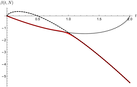
Figure 1: Plot of the GWW beta function $\beta(t,N)$ in (13). The red solid curve shows the exact beta function for $N=20$. The dashed and dotted lines show the strong-coupling and weak-coupling approximations, respectively, at infinite $N$, from (12). The infinite $N$ approximations show spurious zeros at $t=1/2$ and $t=2$, but in fact the true beta function has a single zero at $t=0$. As $N\to\infty$, the jump at $t=1$ shown in the red curve becomes a cusp, indicating the $N=\infty$ third-order phase transition gw ; wadia , and the beta function curve jumps from the infinite $N$ strong-coupling form to the infinite $N$ weak-coupling form as $t$ decreases through the phase transition. See Fig. 2 for a close-up of the cusp at $t=1$. The finite $N$ corrections, which produce this jump, are described in Sec. II in the form of a large $N$ trans-series.

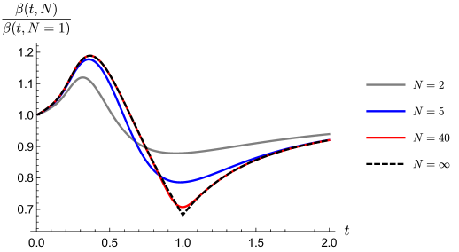
Figure 2: Plot of the ratio of the beta function $\beta(t,N)$ to the $N=1$ beta function, which shows the development, as $N$ increases, of the kink at the $N=\infty$ phase transition point $t=1$.

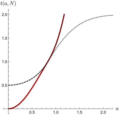
Figure 3: The running coupling $t(a,N)$ [red solid curve] as a function of the lattice scale $a$, for $N=20$. The dashed and dotted curves show the strong coupling and weak coupling behavior, respectively, at infinite $N$. The true behavior of the running coupling jumps from one asymptotic curve to the other, near the $N=\infty$ phase transition point: $t=1$. The finite $N$ corrections, in the form of a large $N$ trans-series, are described in Section III.

II Large N Trans-series for the Beta function

From the definition (4), for any $N$, we compute $\partial_{t}a$ and invert, in order to express the beta function in terms of the Wilson loop:

$$\beta(t,N)=-2\frac{\mathcal{W}(t,N)\,\ln\,\mathcal{W}(t,N)}{\partial_{t}\,\mathcal{W}(t,N)}=\frac{-2}{\partial_{t}\left(\ln\,\ln\mathcal{W}(t,N)\right)}$$ (13)

This implies that the beta function $\beta(t,N)$ inherits its non-perturbative trans-series structure directly from the trans-series structure of the Wilson loop $\mathcal{W}(t,N)$. The large $N$ trans-series for $\mathcal{W}(t,N)$ was studied in ad , showing how the form of the trans-series changes across the phase transition at $t=1$. Related changes therefore occur for the beta function. For other discussions of non-perturbative effects for the GWW Wilson loop, see Okuyama:2017pil ; Alfinito:2017hsh .

We briefly review some relevant results from ad . The non-perturbative trans-series form of $\mathcal{W}(t,N)$ at any $N$ is efficiently expressed in terms of a solution to a Painlevé III equation. Define $\Delta(t,N)$ as the expectation value of the determinant in the Gross-Witten-Wadia model:

$$\Delta(t,N)\equiv\langle\det U\rangle$$ (14)

Then $\mathcal{W}(t,N)$ is related to $\Delta(t,N)$, for any $N$, as:

$$\mathcal{W}(t,N)=\frac{1}{2t}\left[1-\Delta^{2}-\frac{t^{2}}{1-\Delta^{2}}\left(\frac{t^{2}(\partial_{t}\Delta)^{2}}{N^{2}}-1\right)\right]-\frac{t}{2}$$ (15)

The expectation value $\Delta(t,N)$ satisfies the following nonlinear ordinary differential equation, as a function of the ’t Hooft coupling $t$, for any value of $N$ Rossi:1982vw ; Rossi:1996hs ; ad :

$$t^{2}\partial_{t}^{2}\Delta+\frac{N^{2}\Delta}{t^{2}}\left(1-\Delta^{2}\right)=\frac{\Delta}{1-\Delta^{2}}\left(N^{2}-t^{2}\left(\partial_{t}\Delta\right)^{2}\right)$$ (16)

Notice that $N$ appears as a parameter in this equation, thereby enabling a simple analysis of the large $N$ limit, including analytic continuation in $N$. The equation (16) is directly related to the Painlevé III equation, and standard resurgent asymptotic techniques costin-book permit the development of explicit trans-series expansions in various limits: for example, weak or strong ’t Hooft coupling ad .

Combining (13) and (15), the GWW beta function can also be expressed in terms of $\Delta(t,N)$:

$$\beta(t,N) = -2t\left(1-\frac{2\left(\Delta^{2}-1\right)^{2}}{\Delta^{4}-\left(t^{2}+2\right)\Delta^{2}+1+t^{4}(\partial_{t}\Delta)^{2}/N^{2}}\right)$$ (17)

$$\times\ln\left[\frac{1}{2t}\left(1-\Delta^{2}-\frac{t^{2}}{1-\Delta^{2}}\left(\frac{t^{2}(\partial_{t}\Delta)^{2}}{N^{2}}-1\right)\right)-\frac{t}{2}\right]$$

For example, from (16) we see that at infinite $N$

$$\Delta(t,N)\xrightarrow{N\to\infty}\left\{\begin{array}[]{@{}r@{\quad}l@{}}0\text{\qquad\quad strong coupling, }t\geq 1\\ \sqrt{1-t}\text{\qquad\quad weak coupling, }t\leq 1\end{array}\right.$$ (18)

from which follows the infinite $N$ beta function in (12).

The correspondence (17) means that we can use the trans-series structure of $\Delta(t,N)$ to study the trans-series structure of $\beta(t,N)$. And since the trans-series expansions of $\Delta(t,N)$ were shown in ad to display concrete resurgence relations between different non-perturbative sectors in the trans-series, it follows that the same is true for the beta function $\beta(t,N)$.

We can also use the relation (17) to plot the beta function as a function of coupling, for various values of $N$: see Figures 1 and 2. These figures illustrate the fact that for any given $N$, the weak coupling dependence merges consistently with the strong coupling dependence, with a cusp developing at the critical ’t Hooft coupling only at $N=\infty$. In particular, it is clear that the zeros of the infinite $N$ beta function at $t=1/2$ and $t=2$ (see Fig. 1) are indeed spurious.

It is instructive to study the leading trans-series corrections to the infinite $N$ beta functions in (12). The form of the trans-series changes across the phase transition, so we illustrate this change of structure by considering the leading contributions at large but finite $N$. Express the Wilson loop for any finite $N$ as

$$\mathcal{W}=\mathcal{W}_{\rm pert}+\mathcal{W}_{\rm non-pert}$$ (19)

Keeping the leading power of the non-perturbative term, we obtain the following expression for the beta function:

$$\beta(t,N) = -\frac{2\ln\mathcal{W}_{\rm pert}(t,N)}{\partial_{t}\ln\mathcal{W}_{\rm pert}(t,N)}+\dfrac{2}{\partial_{t}\mathcal{W}_{\text{pert}}}\left(\frac{\ln\mathcal{W}_{\rm pert}}{\partial_{t}\ln\mathcal{W}_{\rm pert}}\partial_{t}\mathcal{W}_{\rm non-pert}-\ln\left(e\,\mathcal{W}_{\rm pert}\right)\mathcal{W}_{\rm non-pert}\right)+\dots$$ (20)

$$\equiv \beta_{\rm pert}(t,N)+\beta_{\rm non-pert}(t,N)$$

where the dots refer to higher powers of $\mathcal{W}_{\rm non-pert}$.

II.1 Large N expansion at strong ’t Hooft coupling

In the strong coupling limit, $\Delta_{\rm pert}$ is identically zero, so $\Delta(t,N)$ is purely non-perturbative ad . Consequently, from (15) we deduce that the Wilson loop $\mathcal{W}(t,N)$ has only one perturbative term, $\mathcal{W}_{\rm pert}=\frac{1}{2t}$, which is independent of $N$, and equal to the familiar infinite $N$ Wilson loop in (12). At finite $N$, the further corrections are all non-perturbative. Keeping the leading such non-perturbative correction ad ; Okuyama:2017pil ; Alfinito:2017hsh ,

where the large $N$ instanton action at strong coupling is

$$S_{\rm strong}(t)={\rm arccosh(t)}-\sqrt{1-1/t^{2}}$$ (22)

This translates into a non-perturbative large $N$ instanton correction to the infinite $N$ beta function in (12):

$$\beta_{\text{strong}}(t,N)=-2t\ln(2t)$$ (23)

$$-\dfrac{1}{N\pi}\frac{2t^{2}\ln(2t)}{\sqrt{t^{2}-1}} e^{-2NS_{\text{strong}}(t)}\left(1+\frac{t\left(6t^{2}-6-\left(14t^{2}-9\right)\ln(2t)\right)}{12N\left(t^{2}-1\right)^{3/2}\ln(2t)}+\dots\right)+\dots$$

Note the appearance of further terms involving $\ln(t)$ in the fluctuations about the leading large $N$ instanton term, consistent with general trans-series structure costin-book ; sauzin ; Aniceto:2018bis .

At any finite $N$, the expression (23) has an unphysical divergence at $t=1$, arising from use of the Debye expansion for the Bessel functions dlmf:debye . In ad , the leading large $N$ correction for the Wilson loop at strong coupling was calculated more precisely to be:

$$\mathcal{W}_{\text{strong}}(t,N)\approx\frac{1}{2t}-\frac{1}{2t}\left[\left(J_{N}\left(N/t\right)\right)^{2}-J_{N-1}\left(N/t\right)J_{N+1}\left(N/t\right)\right]+\dots$$ (24)

This leading correction, in terms of Bessel J functions, is exponentially small at large $N$, and represents a resummation of all fluctuations about the leading large $N$ instanton exponential factor in (21). At finite $N$, expression (24) is therefore much more accurate than the conventional large $N$ expression (21) in the vicinity of the large $N$ phase transition, at $t=1$, where instantons and their fluctuations condense ad ; Neuberger:1980as .

A uniform large $N$ instanton expression is obtained by using the uniform large $N$ approximation dlmf-uniform for the Bessel functions appearing in (24). This is a nonlinear analogue of the uniform WKB approximation, smooth through the transition point for any finite $N$, and expressed in terms of an Airy function rather than an exponential ad ; dlmf-uniform . Physically, this uniform large $N$ approximation arises from the merging of two saddles at the large $N$ phase transition. A similar expression, along with a corresponding uniform approximation, can be deduced for the beta function at large $N$, in the strong coupling regime:

$$\beta_{\text{strong}}(t,N)\approx-2t\log(2t)-2t\left(\left(J_{N}\left(N/t\right)\right)^{2}+(2\log(2t)-1)J_{N-1}\left(N/t\right)J_{N+1}\left(N/t\right)\right)+\dots$$ (25)

II.2 Large N expansion at weak ’t Hooft coupling

In the weak coupling regime, the infinite $N$ expression in (18), $\Delta\sim\sqrt{1-t}$, receives both perturbative and non-perturbative corrections at finite $N$:

$$\Delta(t,N)=\Delta_{\rm pert}(t,N)+\Delta_{\rm nonpert}(t,N)$$ (26)

This structure flows through to the Wilson loop and to the beta function.

$$\mathcal{W}_{\text{weak}}(t,N)= \left(1-\frac{t}{2}-\frac{t^{2}}{8N^{2}(1-t)}+\dots\right)$$ (27)

$$-\dfrac{i}{2\sqrt{2\pi}N^{3/2}}\frac{t}{(1-t)^{1/4}}e^{-NS_{\text{weak}}(t)}\left(1+\frac{8+12t+9t^{2}}{96N(1-t)^{3/2}}+\dots\right)$$

where the large $N$ instanton action at weak coupling is

$$S_{\text{weak}}(t)=\frac{2\sqrt{1-t}}{t}-2\,{\rm arctanh}\left(\sqrt{1-t}\right)$$ (28)

The corresponding large $N$ trans-series expansion for the beta function has the form

$$\beta_{\text{weak}}(t,N) = 2(2-t)\log\left(1-\frac{t}{2}\right)\Bigg{[}\left(1-\frac{t\left(t-t^{2}+(4-3t)\ln\left(1-\frac{t}{2}\right)\right)}{4N^{2}(2-t)(1-t)^{2}\log\left(1-\frac{t}{2}\right)}+\dots\right)$$ (29)

$$-i\sqrt{\frac{2}{\pi N}}\frac{(1-t)^{1/4}}{t}e^{-NS_{\text{weak}}(t)}\left(1+\dots\right)+\dots\Bigg{]}$$

II.3 Large N Double-scaling Limit

It is well known that the double-scaling limit is described by the Painlevé II equation gw ; wadia ; marino-matrix . In our approach this can be seen as follows. In the double-scaling limit, zoomed in to the immediate vicinity of the GWW phase transition at $t=1$, the Rossi equation (16) reduces to a Painlevé II equation in terms of the scaled variable $\kappa$ which measures the scaled deviation from $t=1$:

$$t=1+\frac{\kappa}{N^{2/3}}\qquad,\qquad\Delta(t,N)=\frac{t^{1/3}}{N^{2/3}}\,V(\kappa)$$ (30)

Here $V(\kappa)$ is the real Hastings-McLeod solution of the Painlevé II equation marino-matrix ; ad . In this double-scaling limit, the Wilson loop behaves as

$$\mathcal{W}_{\text{double-scaling}}(\kappa)\approx\frac{1}{2}-\frac{\kappa}{2\,N^{2/3}}+\frac{\left(\kappa+V^{2}(\kappa)\right)^{2}-(V^{\prime}(\kappa))^{2}}{2\,N^{4/3}}+\mathcal{O}\left(\frac{1}{N^{2}}\right)$$ (31)

and the beta function as

$$\beta_{\text{double-scaling}}(\kappa) \approx -2\ln(2)$$ (32)

$$-\frac{4\ln 2}{N^{2/3}}\bigg{(}\kappa\frac{\ln(2e)}{2\ln 2}+V^{2}(\kappa)+2\kappa V(\kappa)V^{\prime}(\kappa)+2V^{3}(\kappa)V^{\prime}(\kappa)-V^{\prime}(\kappa)V^{\prime\prime}(\kappa)\bigg{)}$$

$$+\,\mathcal{O}\left(\frac{1}{N^{4/3}}\right)$$

This matches smoothly to the strong- and weak-coupling sides of the phase transition, as shown for the double-scaling limit of $\Delta(t,N)$ in ad .

III Large N Trans-series for the Running Coupling

At infinite $N$, the running coupling has the form in (11). The finite $N$ corrections, described in the previous section for the beta function, lead also to trans-series structures for $t(a,N)$. At strong coupling, where the scale $a$ is large, the corrections are naturally expressed in terms of the Wilson loop, $\mathcal{W}=\exp[-a^{2}]$; while at weak coupling, where the scale $a$ is small, the corrections are naturally expressed in terms of $1-\mathcal{W}=1-\exp[-a^{2}]$. The infinite $N$ phase transition occurs at $\mathcal{W}=1/2$. At any finite $N$, the running coupling, $t(a,N)$ solves the scaling equation

$$a\frac{\partial t}{\partial a}=2\frac{\mathcal{W}(t,N)\,\ln\mathcal{W}(t,N)}{\partial_{t}\mathcal{W}(t,N)}$$ (33)

which is both non-linear and non-perturbative. It is convenient to consider the coupling as a function of the Wilson loop $\mathcal{W}$. At $N=\infty$ we have:

$$t(\mathcal{W},N)\xrightarrow{N\to\infty}\left\{\begin{array}[]{@{}r@{\quad}l@{}}\dfrac{1}{2\mathcal{W}}\text{\qquad\qquad strong coupling, }\mathcal{W}\leq\frac{1}{2}\\ 2(1-\mathcal{W})\text{\qquad weak coupling, }\mathcal{W}\geq\frac{1}{2}\end{array}\right.$$ (34)

By matching the expansions of $\mathcal{W}$, we deduce the following large $N$ trans-series structures for $t$ as a function of $\mathcal{W}$ (and hence of $a$)

$$t(\mathcal{W},N)=\left\{\begin{array}[]{@{}r@{\quad}l@{}}\dfrac{1}{2\mathcal{W}}+\sum_{k=1}^{\infty}e^{-kN\hat{S}_{\text{strong}}(\mathcal{W})}\mathcal{F}^{(k)}_{\text{strong}}(\mathcal{W},N),\text{\quad strong coupling, }\mathcal{W}\leq\frac{1}{2}\\ \sum_{k=0}^{\infty}e^{-kN\hat{S}_{\text{weak}}(\mathcal{W})}\mathcal{F}^{(k)}_{\text{weak}}(\mathcal{W},N),\text{\qquad\qquad weak coupling, }\mathcal{W}\geq\frac{1}{2}\end{array}\right.$$ (35)

The actions $\hat{S}_{\text{strong}}(\mathcal{W})$ and $\hat{S}_{\text{weak}}(\mathcal{W})$ are the strong and weak coupling actions $S_{\text{strong}}(t)$ and $S_{\text{weak}}(t)$, evaluated at the infinite $N$ values of $t$ as given in (34):

$$\hat{S}_{\text{strong}}(\mathcal{W}) =S_{\text{strong}}\left(\dfrac{1}{2\mathcal{W}}\right)={\rm arccosh}\left(\dfrac{1}{2\mathcal{W}}\right)-\sqrt{1-4\mathcal{W}^{2}}$$ (36)

$$\hat{S}_{\text{weak}}(\mathcal{W}) =S_{\text{weak}}\big{(}2(1-\mathcal{W})\big{)}=\dfrac{\sqrt{2\mathcal{W}-1}}{1-\mathcal{W}}-2\,{\rm arctanh}\left(\sqrt{2\mathcal{W}-1}\right)$$

The leading terms in the strong coupling trans-series (35) read:

$$t_{\text{strong}} (\mathcal{W},N)\approx\frac{1}{2\mathcal{W}}$$ (37)

$$-\frac{e^{-N\hat{S}_{\text{strong}}(\mathcal{W})}}{4\pi N^{2}\mathcal{W}\left(1-4\mathcal{W}^{2}\right)}\left(1-\frac{6\mathcal{W}^{2}+7}{6N\left(1-4\mathcal{W}^{2}\right)^{3/2}}-\frac{324\mathcal{W}^{4}+804\mathcal{W}^{2}+85}{72N^{2}\left(1-4\mathcal{W}^{2}\right)^{3}}+\dots\right)+\dots$$

understood as being expanded in $\mathcal{W}=\exp[-a^{2}]$. At weak coupling

$$t_{\text{weak}}(\mathcal{W},N)\approx 2(1-\mathcal{W})\left(1-\frac{1-\mathcal{W}}{2N^{2}(2\mathcal{W}-1)}+\frac{\left(8\mathcal{W}^{2}+5\mathcal{W}-9\right)(1-\mathcal{W})^{2}}{8N^{4}(2\mathcal{W}-1)^{4}}+\dots\right)$$ (38)

$$-\frac{2i}{\pi N^{3/2}}\frac{1-\mathcal{W}}{\left(2\mathcal{W}-1\right)^{1/4}}e^{-N\hat{S}_{\text{weak}}(\mathcal{W})}\left(1-\frac{9\mathcal{W}^{2}+5}{24N(2\mathcal{W}-1)^{3/2}}+\dots\right)+\dots{}$$

understood as being expanded in $(1-\mathcal{W})=(1-\exp[-a^{2}])$.

IV Conclusions

The Gross-Witten-Wadia unitary matrix model is a one-plaquette model of 2 dimensional lattice Yang-Mills theory, which has the interesting feature of a third-order phase transition at infinite $N$, in addition to a running coupling gw ; wadia . The perturbative beta function for this model acquires a non-perturbative trans-series completion at large but finite $N$ in the ’t Hooft limit, as does the running coupling. The ’t Hooft coupling runs with the scale $a$, and the trans-series rearranges itself across the phase transition. Physically, this transition is identified with the condensation of instantons Neuberger:1980as , with different kinds of instantons dominating at weak- and strong-coupling marino-matrix ; Buividovich:2015oju ; Alvarez:2016rmo . Technically, the beta function $\beta(t,N)$ can be expressed explicitly in terms of the expectation value $\Delta(t,N)\equiv\langle\det U\rangle$, whose resurgent trans-series structure was studied in detail in ad . The beta function $\beta(t,N)$ inherits its trans-series structure from that of $\Delta(t,N)$, and therefore the beta function trans-series also has full resurgent properties, including concrete relations between different instanton sectors. It would be interesting to study further this trans-series structure directly in the renormalization group approach to matrix models Carlson:1984nb ; Brezin:1992yc ; Damgaard:1993df ; Higuchi:1993nq .

Acknowledgments: This material is based upon work supported by the U.S. Department of Energy, Office of Science, Office of High Energy Physics under Award Number DE-SC0010339.

References

- (1) G. V. Dunne and M. Ünsal, “New Nonperturbative Methods in Quantum Field Theory: From Large-N Orbifold Equivalence to Bions and Resurgence,” Ann. Rev. Nucl. Part. Sci. 66, 245 (2016), [arXiv:1601.03414].
- (2) D. J. Gross and E. Witten, “Possible Third Order Phase Transition in the Large N Lattice Gauge Theory,” Phys. Rev. D 21, 446 (1980).
- (3) S. R. Wadia, “A Study of U(N) Lattice Gauge Theory in 2-dimensions,” [arXiv:1212.2906], an edited version of the unpublished 1979 preprint, EFI-79/44-CHICAGO.
- (4) E. Brézin and S. R. Wadia, The large N expansion in quantum field theory and statistical physics: from spin systems to 2-dimensional gravity, (World Scientific, 1993).
- (5) P. Rossi, M. Campostrini and E. Vicari, “The Large N expansion of unitary matrix models,” Phys. Rept. 302, 143 (1998), [arXiv:hep-lat/9609003].
- (6) P. Di Francesco, P. Ginsparg and J. Zinn-Justin, “2-D Gravity and random matrices”, Phys. Rept. 254, 1 (1995), [arXiv:hep-th/9306153].
- (7) P. J. Forrester, Log-Gases and Random Matrices, (Princeton Univ. Press, 2010).
- (8) G. Akemann, J. Baik and Ph. Di Francesco, The Oxford handbook of random matrix theory, (Oxford University Press, 2011).
- (9) M. Mariño, Instantons and Large N: An Introduction to Non-Perturbative Methods in Quantum Field Theory, (Cambridge University Press, 2015).
- (10) F. David, “Loop Equations and Nonperturbative Effects in Two-dimensional Quantum Gravity,” Mod. Phys. Lett. A 5, 1019 (1990); “Phases of the large N matrix model and nonperturbative effects in 2-d gravity,” Nucl. Phys. B 348, 507 (1991).
- (11) C. A. Tracy and H. Widom, “Level spacing distributions and the Bessel kernel,” Commun. Math. Phys. 161, 289 (1994), [arXiv:hep-th/9304063]; “Fredholm determinants, differential equations and matrix models,” Commun. Math. Phys. 163, 33 (1994), [arXiv:hep-th/9306042].
- (12) D. J. Gross, “Two-dimensional QCD as a string theory,” Nucl. Phys. B 400, 161 (1993), [arXiv:hep-th/9212149]; D. J. Gross and W. Taylor, “Two-dimensional QCD is a string theory,” Nucl. Phys. B 400, 181 (1993), [arXiv:hep-th/9301068].
- (13) M. R. Douglas and V. A. Kazakov, “Large N phase transition in continuum QCD in two-dimensions,” Phys. Lett. B 319, 219 (1993), [arXiv:hep-th/9305047].
- (14) D. J. Gross and A. Matytsin, “Instanton induced large N phase transitions in two-dimensional and four-dimensional QCD,” Nucl. Phys. B 429, 50 (1994), [arXiv:hep-th/9404004]; “Some properties of large N two-dimensional Yang-Mills theory,” Nucl. Phys. B 437, 541 (1995), [arXiv:hep-th/9410054].
- (15) M. Mariño, “Nonperturbative effects and nonperturbative definitions in matrix models and topological strings,” JHEP 0812, 114 (2008), [arXiv:0805.3033].
- (16) A. Ahmed and G. V. Dunne, “Transmutation of a Trans-series: The Gross-Witten-Wadia Phase Transition,” J. High Energ. Phys. 1711, 054 (2017), [arXiv:1710.01812].
- (17) The Painlevé equations are listed at http://dlmf.nist.gov/32.2.i. For the coalescence cascades, see http://dlmf.nist.gov/32.2.vi.
- (18) K. Okuyama, “Wilson loops in unitary matrix models at finite ,” JHEP 1707, 030 (2017), [arXiv:1705.06542].
- (19) E. Alfinito and M. Beccaria, “Large expansion of Wilson loops in the Gross-Witten-Wadia matrix model,” J. Phys. A 51, no. 5, 055401 (2018), [arXiv:1707.09625].
- (20) P. Rossi, “On The Exact Evaluation Of Det U(p) In A Lattice Gauge Model,” Phys. Lett. 117B, 72 (1982).
- (21) O. Costin, Aymptotics and Borel Summability, (CRC Press, 2008).
- (22) C. Mitschi and D. Sauzin, Divergent Series, Summability and Resurgence I, Lecture Notes in Math 2153 (Springer, 2016).
- (23) I. Aniceto, G. Basar and R. Schiappa, “A Primer on Resurgent Transseries and Their Asymptotics,” arXiv:1802.10441.
- (24) For the Debye large approximation to Bessel functions, see http://dlmf.nist.gov/10.19.ii.
- (25) H. Neuberger, “Instantons as a bridgehead at N = infinity,” Phys. Lett. 94B, 199 (1980); “Nonperturbative Contributions in Models With a Nonanalytic Behavior at Infinite ,” Nucl. Phys. B 179, 253 (1981).
- (26) For the uniform large approximation to Bessel functions, see http://dlmf.nist.gov/10.20.
- (27) P. V. Buividovich, G. V. Dunne and S. N. Valgushev, “Complex Path Integrals and Saddles in Two-Dimensional Gauge Theory,” Phys. Rev. Lett. 116, no. 13, 132001 (2016), [arXiv:1512.09021].
- (28) G. Álvarez, L. Martínez Alonso and E. Medina, “Complex saddles in the Gross-Witten-Wadia matrix model,” Phys. Rev. D 94, no. 10, 105010 (2016), [arXiv:1610.09948].
- (29) J. W. Carlson, “Approaching the Large Limit: A Renormalization Group Approach to Large Field Theories,” Nucl. Phys. B 248, 536 (1984).
- (30) E. Brezin and J. Zinn-Justin, “Renormalization group approach to matrix models,” Phys. Lett. B 288, 54 (1992) [arXiv:hep-th/9206035].
- (31) P. H. Damgaard and U. M. Heller, “On spin and matrix models in the complex plane,” Nucl. Phys. B 410, 494 (1993), [arXiv:hep-lat/9307016].
- (32) S. Higuchi, C. Itoi, S. Nishigaki and N. Sakai, “Nonlinear renormalization group equation for matrix models,” Phys. Lett. B 318, 63 (1993), [arXiv:hep-th/9307116]; “Renormalization group flow in one and two matrix models,” Nucl. Phys. B 434, 283 (1995), Erratum: [Nucl. Phys. B 441, 405 (1995)], [arXiv:hep-th/9409009].