Neural-network states for the classical simulation of quantum computing

Abstract

Simulating quantum algorithms with classical resources generally requires exponential resources. However, heuristic classical approaches are often very efficient in approximately simulating special circuit structures, for example with limited entanglement, or based on one-dimensional geometries. Here we introduce a classical approach to the simulation of general quantum circuits based on neural-network quantum states (NQS) representations. Considering a set of universal quantum gates, we derive rules for exactly applying single-qubit and two-qubit $Z$ rotations to NQS, whereas we provide a learning scheme to approximate the action of Hadamard gates. Results are shown for the Hadamard and Fourier transform of entangled initial states for systems sizes and total circuit depths exceeding what can be currently simulated with state-of-the-art brute-force techniques. The overall accuracy obtained by the neural-network states based on Restricted Boltzmann machines is satisfactory, and offers a classical route to simulating highly-entangled circuits. In the test cases considered, we find that our classical simulations are comparable to quantum simulations affected by an incoherent noise level in the hardware of about $10^{-3}$ per gate.

Introduction.-

Quantum algorithms offer exponential speedup over the best known classical algorithms for several interesting problems, ranging from quantum simulation Feynman82simulatingphysics ; lloyd_universal_1996 to integer factoring shor_polynomial-time_1997 . While the origin of the speedup varies from one quantum algorithm to another divincenzo_quantum_1995 ; RevModPhys.82.1 , an essential ingredient is the ability to efficiently modify and retrieve information stored in the large Hilbert space in which the quantum wave function lives. With quantum computers being actively developed neumann_multipartite_2008 ; mariantoni_implementing_2011 ; johnson_quantum_2011 ; blatt_quantum_2012 ; debnath_demonstration_2016 ; kandala_hardware-efficient_2017 ; hempel_quantum_2018 , it is becoming crucial to understand what practical applications these platforms should target, and what problems instead are better suited for classical algorithms. Indeed, delineating the so-called “quantum supremacy”–the point at which a quantum computer has solved a problem that a classical computer cannot solve in the foreseeable future–is a topic of very active current research Lund2017 ; Harrow2017 that pushes the limits of classical computation Boixo2018 ; boixo2017 ; haener2017 ; pednault2017 ; chen2018 ; chen2018b ; li2018 . To this end, useful guidance can be obtained from a comprehensive understanding of which interesting quantum algorithms that can be efficiently approximated using classical computers.

At first sight, the nominal exponential complexity of a generic quantum state suggests that efficient classical simulation of large quantum algorithms is impossible. However, in several interesting applications the practical complexity of the quantum state is greatly reduced, and heuristic classical approaches can be extremely successful at simulating the circuit at hand. Several classical approaches exploit the explicit structure of specific quantum circuits to provide polynomially, or effectively polynomially scaling simulation algorithms. Noticeable examples are circuits that are constituted of Clifford group gates 1998quant.ph..7006G ; jozsa_matchgates_2008 ; jozsa_jordan-wigner_2015 , entanglement-limited circuits Jozsa2011 ; PhysRevLett.91.147902 , and circuits with restricted topological and depth properties 2005quant.ph.11069M ; PhysRevLett.96.170503 ; 2006quant.ph..3163J ; van_den_nest_simulating_2011 . In addition, techniques originally developed in the context of many-body quantum theory can be also used to efficiently simulate specific classes of quantum circuits. Particularly successful are approaches based on Matrix Product States (MPS) white_density_1992 ; fannes1992 ; ostlund1995 , allowing to efficiently simulate the Quantum Fourier Transform of initial states of manageable bond dimension, typically arising in 1D physical systems 2007NJPh….9..146B . Of course these approaches cannot work in general, and there are thus many quantum algorithms of interest for which efficient classical algorithms are unknown. These most chiefly include quantum algorithms involving high entanglement, and with underlying geometries beyond the one-dimensional case amenable to MPS simulations. In this paper, we ask how we can extend the current abilities of classical simulation in these situations.

In recent times, machine learning techniques have been introduced as a novel approach to simulate highly entangled quantum systems. Key component of these approaches is a compact representation of the many-body quantum state, based on artificial neural networks carleo_solving_2016 . This approach has so far been used for the simulation of systems relevant for many-body quantum theory, including spins deng_quantum_2017 ; glasser_neural-network_2018 ; choo_symmetries_2018 ; kaubruegger_chiral_2018 ; carleo_constructing_2018 , bosons saito_machine_2017 ; saito_method_2018 ; saito_solving_2017 ; choo_symmetries_2018 , and fermions nomura_restricted-boltzmann-machine_2017 . Having a compact representation of the many-body state naturally leads to applications to quantum computing. For example, neural-network representations of quantum states have been used to learn many-qubit states from experimental measurements. Given the success in efficiently reconstructing the state of possibly large quantum computers torlai_neural-network_2018 ; rocchetto_learning_2018 ; torlai_latent_2018 , and highly-entangled states deng_exact_2016 ; deng_quantum_2017 ; chen_equivalence_2017 , it is natural to ask whether a classical algorithms based on artificial neural networks and stochastic learning can be devised to simulate quantum circuits.

In this paper, we present a general method to approximate the unitary transformations that comprise quantum circuits using neural-network quantum states based on complex-valued restricted Boltzmann machines and Monte Carlo sampling. This is achieved via a stochastic framework to learn the target quantum state after each gate in the circuit. In particular, we demonstrate the effectiveness of the method on fundamental primitives of quantum algorithms, such as the Hadamard and the Quantum Fourier transforms. As non-trivial entangled test input states, we consider the critical ground states of the transverse field Ising model (TFIM) in both one and two dimensions.

Neural-network states.-

Consider a quantum system consisting of $N$ qubits. Here we use a representation of the many-body state associated to this system in terms of a neural-network quantum state (NQS). More specifically, we consider a Restricted Boltzmann machine (RBM) architecture Hinton02 ; hinton_reducing_2006 ; lecun_deep_2015 . The RBM consists of a visible layer of $N$ nodes corresponding to the qubit degrees of freedom, and a layer of M latent variables ($h_{1},h_{2},...,h_{M}$). In the following, we work in the basis of eigenstates of the Pauli $Z$ operator on each site, and specify a basis state through bitstrings $|\mathcal{B}\rangle\equiv|B_{1},B_{2},...,B_{N}\rangle$. Here the $B$ variables are quantum numbers that can take the values $\left\{0,1\right\}$, and $Z|B\rangle=(-1)^{B}|B\rangle$. Given an input bitstring $\mathcal{B}$, the RBM is taken to output a complex number corresponding to the unnormalized wave-function amplitude $\langle\mathcal{B}|\Psi\rangle\equiv\Psi(\mathcal{B})$. This network description corresponds to the following variational expression for the quantum states carleo_solving_2016 :

$$\Psi_{\mathcal{W}}(\mathcal{B})=\exp\left(\sum_{j}^{N}a_{j}B_{j}\right)\times\\ \times\prod_{k}^{M}\left[1+\exp\left(b_{k}+\sum_{j}W_{jk}B_{j}\right)\right],$$ (1)

where the lower-script $\mathcal{W}$ denotes the dependence on a set of complex variational parameters, including the visible bias $a_{j}$, the hidden bias $\beta_{k}$ and the weights $W_{jk}$.

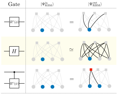
Figure 1: Action of a set of universal gate on a restricted Boltzman machine state. Here, $|\Psi_{\mathrm{RBM}}^{\mathrm{in}}\rangle$ represents the input state to which the gates in leftmost column are applied, $|\Psi_{\mathrm{RBM}}^{\mathrm{out}}\rangle$ is instead the output state. Single-qubit $Z$ rotations (upper panels) acting on a given qubit (in blue) result in local weight modifications, $\mathrm{CR^{Z}(\phi)}$ gates (bottom panels) acting on two qubits (in blue) require instead the introduction of an extra hidden neuron (in red). Those two families of gates can be applied exactly, whereas the Hadamard gate (middle panels) is approximated through the numerical scheme described in the text.

We then consider a quantum circuit, whose action is fully specified by a sequence of $N_{g}$ local gates $\mathcal{G}_{p}$ where $p=1,..,N_{g}$. Any unitary operation and hence any quantum circuit can be approximated to arbitrary accuracy in terms of a set of universal gates. In the following, we consider the universal set of gates comprising single-qubit rotations around the $Z$ axis ($R^{Z}(\phi)$), the Hadamard gate ($H$) and controlled rotations around the $Z$ axis ($\mathrm{CR^{Z}(\phi)}$). In order to simulate quantum computing with a neural-network ansatz, we then devise strategies to apply such gates to the states (1). Specifically, for a given gate $\mathcal{G}_{p}$ we look for a solution to $\langle\mathcal{B}|\Psi_{\mathcal{W^{\prime}}}\rangle=\langle\mathcal{B}|\mathcal{G}_{p}|\Psi_{\mathcal{W}}\rangle$, where the new set of weights $\mathcal{W^{\prime}}$ should be determined in such a way that this equation is satisfied for all the possible values of bistrings $\mathcal{B}$.

For the particular choice of NQS used here, all gates that are diagonal in the computational basis can easily be applied exactly. In the case, of single-qubit gates, these are (up to irrelevant global phases) all given by the diagonal matrix $R^{z}(\phi)=\mathrm{Diag(1,e^{i\phi})}$. The action of $R^{Z}(\phi)$ on a given qubit $l$ yields amplitudes $\langle\mathcal{B}|R_{l}^{Z}(\phi)|\Psi_{\mathcal{W}}\rangle=e^{iB_{l}\phi}\Psi_{\mathcal{W}}(\mathcal{\mathcal{B}})$. The action of the gate can be exactly reproduced with the choice $\mathcal{W}^{\prime}=\{\alpha^{\prime},\beta,W\}$, where $a_{j}^{\prime}=a_{j}+\delta_{jl}i\phi.$ For two qubits, we consider the controlled $Z$ rotations, and together with the single-qubit rotations generate all diagonal gates. Their action on a given state, $\langle\mathcal{B}|\mathrm{CR^{Z}}_{lm}(\phi)|\Psi_{\mathcal{W}}\rangle=e^{iB_{l}B_{m}\phi}\Psi_{\mathcal{W}}(\mathcal{\mathcal{B}})$, can also be exactly satisfied, apart from a trivial global normalization constant, by introducing an extra hidden unit $h_{[c]}$ coupled only to qubits $l$ and $m$ through the weights $W_{l[c]}=-W_{m[lm]}=2A(\phi)$, with $A(\phi)=\mathrm{arcosh}(e^{-i\phi/2})$ as derived in detail in the Appendix. Also, this gate requires a change in the visible bias, in such a way that $a_{l}^{\prime}=a_{l}+i\phi/2-A(\phi)$ and $a_{m}^{\prime}=a_{m}+i\phi/2+A(\phi)$. Note that the maximum number of hidden units that need to be added to implement all such two-qubit gates is $N^{2}$. The action of circuits containing only $R^{Z}(\phi)$ and $\mathrm{CR^{Z}(\phi)}$ gates thus can be efficiently simulated in terms of RBM states, since it induces local network modifications which are easily determined using the rules discussed above (see Fig. 1 for a schematic representation of how the RBM state is modified in those cases).

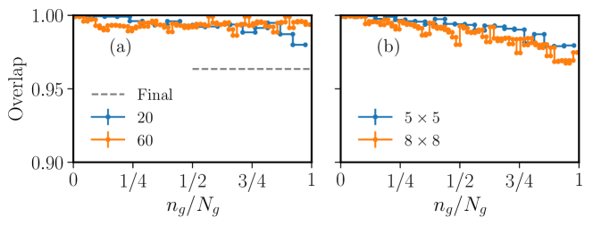
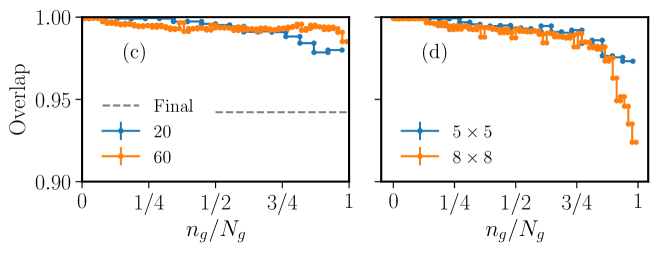
Figure 2: Simulation of quantum transforms with neural-network quantum states. Hadamard transform results are shown in (a,b), whereas Truncated Fourier Transform results are shown in (c,d). Input for the transforms are the ground-states of the Transverse-Field Ising model for one-dimensional chains with periodic boundaries (a,c) and two-dimensional square lattices (b,d). Values of the transverse field are chosen to be at or close to the critical points, thus $\Gamma/J=1$ and $\Gamma/J=3$, respectively. Dots connected by continuous lines show the intermediate fidelities obtained when approximate the action of the Hadamard gates in the circuit. $N_{\mathrm{g}}$ denotes here the total number of Hadamard gates applied. The horizontal dashed lines shown the final overlap between the NQS approximation at the end of the circuit, and the exact state, obtained for the smaller system size ($N=20$ for one-dimensional chains).

Approximating Hadamard gates.-

In order to provide a complete scheme for the classical simulation of quantum circuits with NQS, we further need to specify the action of the Hadamard gate. In contrast to the previously discussed unitaries, in the general case it is hard to find exact strategies to efficiently apply the Hadamard gate to an NQS. The exact application of the Hadamard gate results in the introduction of an additional layer in the Boltzmann machine, thus going beyond the NQS form gao_efficient_2017 . As a consequence of the additional deep layer, the sampling from the evolved states quickly becomes intractable as the circuit depth grows. Here, we instead consider an approximate strategy, relying on a generalized variational treatment of the quantum circuit in the pure RBM form. Given an initial variational state $|\Psi_{\mathcal{W}}\rangle$, our goal is to devise an efficient numerical scheme to obtain an optimal representation of the many-body quantum state after the Hadamard gate, $|\Phi\rangle=H|\Psi_{\mathcal{W}}\rangle$, such that $|\Psi_{\mathcal{W}^{\prime}}\rangle\simeq|\Phi\rangle$ for a set of parameters $\mathcal{W}^{\prime}$ to be determined. Specifically, we consider the negative log-overlap:

$$L(\Psi_{\mathcal{W}^{\prime}},\Phi)=-\log\left[\frac{|\langle\Psi_{\mathcal{W^{\prime}}}|\Phi\rangle|}{||\Psi_{\mathcal{W}^{\prime}}\rangle|||\Phi\rangle|}\right],$$ (2)

which attains a minimum $L=0$ when the two states are equal, and devise a procedure to minimize it with respect to $\mathcal{W^{\prime}}$. In the language of machine learning, this corresponds to the loss function. In analogy with the time-dependent variational Monte Carlo scheme carleo_localization_2012 ; carleo_light-cone_2014 , this quantity can be minimized using a stochastic procedure. In particular, the gradient with respect to the $k$-th variational parameter, $p_{k}$, can expressed in terms of expectation values:

$$\partial_{p_{k}}L(\Psi_{\mathcal{W}^{\prime}},\Phi) = \langle\mathcal{O}_{k}^{\star}(\mathcal{B})\rangle_{\Psi}-\frac{\left\langle\frac{\Phi(\mathcal{B})}{\Psi(\mathcal{B})}\mathcal{O}_{k}^{\star}(\mathcal{B})\right\rangle_{\Psi}}{\left\langle\frac{\Phi(\mathcal{B})}{\Psi(\mathcal{B})}\right\rangle_{\Psi}},$$ (3)

where we have introduced the variational operators $\mathcal{O}_{k}(\mathcal{\mathcal{B}})=\partial_{p_{k}}\log\Psi_{\mathcal{W}^{\prime}}(\mathcal{B})$, and $\langle F(\mathcal{B})\rangle_{\Psi}\equiv\sum_{\mathcal{B}}F(\mathcal{B})|\Psi(\mathcal{B})|^{2}/\sum_{\mathcal{B}}|\Psi(\mathcal{B})|^{2}$ denote expectation values over the variational state $\Psi_{\mathcal{W^{\prime}}}$. The minimization of the negative log-overlap with respect to the parameters of the RBM is then achieved through an iterative scheme where at each iteration stochastic estimates of the gradient are obtained through Eq. (3). The network parameters are then updated with a Stochastic Gradient Descent optimization method kingma_adam:_2014 . This stochastic approach can then be used to systematically optimize the log-overlap even on large systems, inaccessible to exact simulation approaches. Details concerning the sampling procedure, and the optimization steps are discussed in the Appendix.

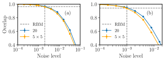
Figure 3: Comparing the effect of hardware noise to the variational error. Continuous lines show the behavior of the overlap as a function of the noise level in a minimal model consisting of depolarizing channels after each gate. The noise model is applied only to the quantum transforms, whereas the preparation of the initial state is assumed to be exact in the hardware. Results are shown for both the Hadamard (a) and the truncated Fourier (b) transforms. Horizontal dashed lines correspond to the NQS final overlap for the smaller 1d systems.

Hadamard and Fourier transform.-

To validate the effectiveness of this scheme in approximating prototypical quantum circuits, we benchmark our approach on the simulation of quantum transforms of entangled initial states. Specifically, the initial states are prepared considering the transverse-field Ising Hamiltonian:

$$\mathcal{H} = -\Gamma\sum_{i}X_{i}+J\sum_{\langle i,j\rangle}Z_{i}Z_{j},$$ (4)

where the interaction terms runs over pairs of nearest neighbors on a lattice. These states exemplify quantum states commonly encountered in quantum simulation. We consider both one-dimensional chains and two-dimensional square lattices with periodic boundary conditions, and prepare an initial NQS in the ground-state of $\mathcal{H}$ at or close to the critical point ($\Gamma/J=1$ in 1d, and $\Gamma/J=3$ for the 2d square lattice). We prepare NQS variational ground states with $\alpha=1$, which in previous work was already shown to yield an accurate description of the ground-state, $|\Phi_{0}\rangle$.

The first transform we consider is the Hadamard transform, in which the output state is given by $|\Phi_{HT}\rangle=H_{1}\dots H_{N}|\Phi_{0}\rangle$, i.e. the corresponding quantum circuits contains Hadamard gates on each qubit. We further apply our approach to the quantum Fourier transform, one of the fundamental building blocks for the most important quantum algorithms, including Shor shor_polynomial-time_1997 , phase estimation kitaev_quantum_1995 , and more Nielsen:2011:QCQ:1972505 . For simplicity, we have considered here the truncated Fourier transform, where the final state is given by $|\Phi_{\mathrm{TFT}}\rangle=H_{N}\dots B_{2,4}A_{2,3}H_{2}B_{1,3}A_{1,2}H_{1}|\Phi_{0}\rangle,$where the controlled gates are $A=\mathrm{CR^{Z}}(\pi/2)$ and $B=\mathrm{CR^{Z}}(\pi/4)$.

Numerical results for the Hadamard transform are shown in Fig. 2 (a,b), and in (c,d) for the truncated Fourier transform. Results for both one- and two-dimensional initial states are presented. The intermediate fidelity, as obtained stochastically minimizing (2) at each step involving an Hadamard gate is shown as a function of the total circuit depth. For both one and two-dimensional circuits we find satisfactorily high intermediate overlaps ($>0.96$) with RBM states of fixed number of hidden units, $\alpha=1$. To the best of our knowledge, the circuits shown here for the largest systems cannot be exactly simulated with existing state-of-the-art brute-force approaches.

In order to assess the overall quality of the variational approximation, beyond the individual gates fidelity, for small one-dimensional systems we compute the overlap between the exact output state and the approximate output variational state (horizontal dashed lines). As expected, the overall fidelity is lower than the intermediate ones, yet not significantly lower than what found for the intermediate steps. Note in particular that the fidelity at the end is better than the product of the intermediate fidelities over the whole evolution, suggesting that there is a cancellation of errors in the final state.

Noisy quantum computing.-

One of the major challenges for quantum computers is controlling and mitigating the effect of noise caused by interactions of the quantum system with the environment. As a result of such decoherence, the output of a quantum computer is affected by a loss of fidelity with the exact target state, if error correction is not taken into account. It is therefore interesting to compare the variational error in the classical NQS simulation to the error due to a noisy quantum hardware. To simulate the effect of noise, we consider here a simple Pauli noise channel, which approximates the depolarizing channel knill_randomized_2008 ; barends_superconducting_2014 ; barends_digitized_2016 . This is implemented by applying, after each one qubit gate, with probability $r$one of the three randomly selected Pauli operators and with probability $1-r$ the qubit is left untouched. For the two-qubit gates one of the 15 combinations of Pauli operators, where the identity on one of the qubits is included, is applied with probability $r$ and the qubit pair is left untouched with probability $1-r$. Here the parameter r has the role of a noise level. Results are shown in Fig. 3 for both the Hadamard transform (a) and the truncated Fourier transform (b). We find similar qualitative and quantitative behavior of the final overlap versus the noise level for both one and two-dimensional initial states. The final overlap achieved with the RBM variational ansatz in 1d is shown as horizontal dashed lines, and correspond to an effective noise level of about $10^{-3}$. Notice that the noise model considered here takes into account hardware error only for the quantum transforms circuits, and not for the circuits necessary to prepare the initial states. The effective noise level for the complete circuits is expected to be significantly lower than $10^{-3}$.

Discussion.-

We have introduced a stochastic algorithm to perform classical simulation of large, entangled quantum circuits. Our results show that neural-network quantum states can approximate, with good fidelity, quantum circuits beyond the current state of the art of brute-force classical simulation. Our approach, while not expected to be efficient in cases where sampling from the wave-function is practically hard, effectively enlarge the space of interesting quantum algorithms that can be classically simulated. Apart from the practical applications of our algorithm, several conceptual points will hopefully be stimulated by our results. For example, the theoretical analysis of the complexity of quantum algorithms might find new insights coming from highly-entangled classical variational representations of the quantum states. Finally, the results presented here can serve as a guide for the undergoing development of quantum hardware, setting reference values for the maximum noise levels necessary to outperform classical approximation schemes.

Appendix A Exact Application of Quantum Gates to Restricted Boltzmann Machines

In this Appendix we discuss a number of quantum gates whose application to an RBM state can be performed efficiently. These include all the single-qubit Pauli gates and Z rotations, as well as two-qubit controlled Z rotations.

A.1 Single-Qubit Z rotations

The action of the single-qubit Z rotations of angle $\phi$ is fully determined by the $2\times 2$ unitary matrix

$$R^{Z}(\phi) = \left(\begin{array}[]{cc}1&0\\ 0&e^{i\phi}\end{array}\right)$$

Its action on a given qubit $l$ yields $\langle\mathcal{B}|R_{l}^{z}(\phi)|\Psi_{\mathcal{W}}\rangle=e^{i\phi B_{l}}\Psi_{\mathcal{W}}(\mathcal{\mathcal{B}})$. Considering a RBM machine with weights $\mathcal{W}^{\prime}=\{\alpha,\beta,W\}$, the action of the $R^{Z}(\phi)$ gate is exactly reproduced if we satisfy $e^{B_{l}a_{l}}e^{i\phi B_{l}}=e^{B_{l}a_{l}^{\prime}},$ which has the simple solution:

$$a_{j}^{\prime} = a_{j}+\delta_{jl}i\phi.$$ (6)

The action of this gate then simply modifies the local visible bias of the RBM.

A.2 Controlled Z rotations

The action of a controlled Z rotations acting on two given qubits $l$ and $m$ is determined by the $4\times 4$ unitary matrix:

$$\mathrm{CR^{Z}}(\phi) = \left(\begin{array}[]{cccc}1&0&0&0\\ 0&1&0&0\\ 0&0&1&0\\ 0&0&0&e^{i\phi}\end{array}\right),$$ (11)

where $\phi$ is a given rotation angle. This gate is diagonal, and we can compactly write it as an effective two-body interaction:

$$\left\langle\mathcal{B}\right|\mathrm{CZ}(\phi)\left|\Psi_{\mathcal{W}}\right\rangle = e^{i\phi B_{l}B_{m}}\Psi_{\mathcal{W}}(Z_{1}\dots Z_{N}).$$ (12)

Since in the RBM architecture there is no direct interaction between visible spins, this CZ interaction can be mediated through the insertion of a dedicated extra hidden unit $h_{c}$, which is coupled only to the qubits $l$ and $m$:

$$\left\langle\mathcal{B}\right|\mathrm{CZ}(\phi)\left|\Psi_{\mathcal{W}}\right\rangle = e^{\Delta a_{l}B_{l}+\Delta a_{m}Z_{m}}\sum_{h_{c}}e^{W_{lc}B_{l}h_{c}+W_{mc}B_{m}h_{c}}$$ (14)

$$= e^{\Delta a_{l}B_{l}+\Delta a_{m}B_{m}}\times$$

$$\times(1+e^{W_{lc}B_{l}+W_{mc}B_{m}})\Psi_{\mathcal{W}}(\mathcal{B}),$$

where the new weights $W_{lc}$ and $W_{mc}$ , and visible units biases $a_{l}^{\prime}=a_{l}+\Delta a_{l}$, $a_{m}^{\prime}=a_{m}+\Delta a_{m}$ are determined by the equation:

$$e^{\Delta a_{l}B_{l}+\Delta a_{m}B_{m}}(1+e^{W_{lc}B_{l}+W_{mc}B_{m}}) = C\times e^{i\phi B_{l}B_{m}},$$ (15)

for all the 4 possible values of the qubits values $B_{l},B_{m}=\{0,1\}$ and where $C$ is an arbitrary (finite) normalization. A possible solution for this system is:

$$W_{lc} = -2\mathcal{A}(\phi)$$ (16)

$$W_{mc} = 2\mathcal{A}(\phi)$$ (17)

$$\Delta a_{l} = i\frac{\phi}{2}+\mathcal{A}(\phi)$$ (18)

$$\Delta a_{m} = i\frac{\phi}{2}-\mathcal{A}(\phi),$$ (19)

where $\mathcal{A}(\phi)=\mathrm{arccosh}\left[e^{-i\frac{\phi}{2}}\right]$.

A.3 Pauli X gate

We then consider an $X$ gate, acting on some given qubit $l$. In this case, the gate just flips the qubit, and the RBM amplitudes are:

$$\langle\mathcal{B}|X_{l}|\Psi_{\mathcal{W}}\rangle = \langle B_{1}\dots\bar{B}_{l}\dots B_{N}|\Psi_{\mathcal{W}}\rangle,$$

therefore since $\bar{B}_{l}=(1-B_{l})$, we must satisfy

$$(1-B_{l})W_{lk}+b_{k} = B_{l}W_{lk}^{\prime}+b_{k}^{\prime},$$ (20)

$$(1-B_{l})a_{l} = B_{l}a_{l}^{\prime}+C,$$ (21)

for all the (two) possible values of $B_{l}=0,1$. The solution is simply:

$$W_{lk}^{\prime} = -W_{lk}$$ (22)

$$b_{k}^{\prime} = b_{k}+W_{lk}$$ (23)

$$a_{l}^{\prime} = -a_{l}$$ (24)

$$C = a_{l}.$$ (25)

whereas all the $a_{j}$ and the other weights $W_{jk}$ with $j\neq l$ are unchanged.

A.4 Pauli Y gate

A similar solution is found also for the Y gate, with the noticeable addition of extra phases with respect to the $X$ gate:

$$W_{lk}^{\prime} = -W_{lk}$$ (26)

$$b_{k}^{\prime} = b_{k}+W_{lk}$$ (27)

$$a_{l}^{\prime} = -a_{l}+i\pi$$ (28)

$$C = a_{l}+\frac{i\pi}{2}.$$ (29)

whereas all the $a_{j}$ and the other weights $W_{jk}$ with $j\neq l$ are unchanged.

A.5 Pauli Z gate

For a $Z$ gate acting on qubit $l$, we have:

$$\langle\mathcal{B}|Z_{l}|\Psi_{\mathcal{W}}\rangle = (-1)^{B_{l}}\langle\mathcal{B}|\Psi_{\mathcal{W}}\rangle,$$ (30)

therefore we must satisfy $e^{B_{l}a_{l}}(-1)^{B_{l}}=e^{B_{l}a_{l}^{\prime}},$ which has the simple solution:

$$a_{l}^{\prime} = a_{l}+i\pi,$$ (31)

whereas all the other weights and biases are unchanged.

Appendix B Stochastic Approximation of the Hadamard Gate

The key numerical component of our approach is the stochastic framework needed to find network parameters $\mathcal{W}^{\prime}$ such that $|\Psi_{\mathcal{W}^{\prime}}\rangle\simeq|\Phi\rangle$ , where $|\Phi\rangle=H_{l}|\Psi_{\mathcal{W}}\rangle$ is the exact state after a Hadamard gate has been applied on some qubit $l$. The overlap between the two states is the key quantity to measure how close these two states are, and reads

$$\mathrm{O}(\mathcal{W}^{\prime}) = \sqrt{\frac{|\langle\Psi_{\mathcal{W}^{\prime}}|\Phi\rangle|^{2}}{\langle\Psi_{\mathcal{W}^{\prime}}|\Psi_{\mathcal{W}^{\prime}}\rangle\langle\Phi|\Phi\rangle}}$$ (32)

$$= \sqrt{\left\langle\frac{\Phi(\mathcal{B})}{\Psi_{\mathcal{W}^{\prime}}(\mathcal{B})}\right\rangle_{\Psi}\left\langle\frac{\Psi_{\mathcal{W}^{\prime}}(\mathcal{B})}{\Phi(\mathcal{B})}\right\rangle_{\Phi}^{\star}},$$

where $\langle F(\mathcal{B})\rangle_{A}\equiv\sum_{\mathcal{B}}F(\mathcal{B})|A(\mathcal{B})|^{2}/\sum_{\mathcal{B}}|A(\mathcal{B})|^{2}$ denote expectation values over the variational state ($A(\mathcal{B})=\Psi_{\mathcal{W^{\prime}}}(\mathcal{B})$) and over the exact state $(A(\mathcal{B})=\Phi(\mathcal{B}))$, respectively. In order to stochastically compute the overlap, we then generate two independent set of samples, one distributed according to $|\Psi_{\mathcal{W^{\prime}}}(\mathcal{B})|^{2}$ and another one according to $|\Phi(\mathcal{B})|^{2}$. These can be obtained using standard Markov Chain Monte Carlo techniques becca_quantum_2017 , and look-up tables approaches as discussed in Ref. carleo_solving_2016 are used to reduce the overall computational complexity of the sampling.

In addition to a stochastic expression for the overlap, it is also possible to find a suitable stochastic expression for its derivatives with respect to a generic network-parameter $k$. In practice, it is more convenient to define as a loss function to be minimized:

$$L(\mathcal{W}^{\prime}) = -\log\mathrm{O}(\mathcal{W}^{\prime}),$$ (33)

which attains a minimum $(L=0$) when the two states are equal. In this case, the gradients have a more compact form than for the bare overlap, and read:

$$\partial_{p_{k}}L(\Psi_{\mathcal{W}^{\prime}}) = \langle\mathcal{O}_{k}^{\star}(\mathcal{B})\rangle_{\Psi}-\frac{\left\langle\frac{\Phi(\mathcal{B})}{\Psi(\mathcal{B})}\mathcal{O}_{k}^{\star}(\mathcal{B})\right\rangle_{\Psi}}{\left\langle\frac{\Phi(\mathcal{B})}{\Psi(\mathcal{B})}\right\rangle_{\Psi}},$$ (34)

where $\mathcal{O}_{k}(\mathcal{\mathcal{B}})=\partial_{p_{k}}\log\Psi_{\mathcal{W}^{\prime}}(\mathcal{B})$ are the variational derivatives, and estimates of the gradient can be obtained sampling according to $|\Psi_{\mathcal{W^{\prime}}}(\mathcal{B})|^{2}$.

Once the loss function and its gradient are defined, we can use any standard Stochastic Gradient Descent method to carry on the optimization. In our results, we have used AdaMax kingma_adam:_2014 , and typically initialized the parameters in a way that $\mathcal{W^{\prime}\simeq\mathcal{W}}$, adding some small random noise to $\mathcal{W}$.

References

- (1) Feynman, R. P. Simulating physics with computers. International Journal of Theoretical Physics 21, 467–488 (1982). URL https://link.springer.com/article/10.1007/BF02650179.
- (2) Lloyd, S. Universal Quantum Simulators. Science 273, 1073–1078 (1996). URL http://science.sciencemag.org/content/273/5278/1073.
- (3) Shor, P. Polynomial-Time Algorithms for Prime Factorization and Discrete Logarithms on a Quantum Computer. SIAM Journal on Computing 26, 1484–1509 (1997). URL https://epubs.siam.org/doi/10.1137/S0097539795293172.
- (4) DiVincenzo, D. P. Quantum Computation. Science 270, 255–261 (1995). URL http://science.sciencemag.org/content/270/5234/255.
- (5) Childs, A. M. & van Dam, W. Quantum algorithms for algebraic problems. Rev. Mod. Phys. 82, 1–52 (2010). URL https://link.aps.org/doi/10.1103/RevModPhys.82.1.
- (6) Neumann, P. et al. Multipartite Entanglement Among Single Spins in Diamond. Science 320, 1326–1329 (2008). URL http://science.sciencemag.org/content/320/5881/1326.
- (7) Mariantoni, M. et al. Implementing the Quantum von Neumann Architecture with Superconducting Circuits. Science 334, 61–65 (2011). URL http://science.sciencemag.org/content/334/6052/61.
- (8) Johnson, M. W. et al. Quantum annealing with manufactured spins. Nature 473, 194–198 (2011). URL http://www.nature.com/nature/journal/v473/n7346/full/nature10012.html.
- (9) Blatt, R. & Roos, C. F. Quantum simulations with trapped ions. Nature Physics 8, 277–284 (2012). URL http://www.nature.com/nphys/journal/v8/n4/abs/nphys2252.html.
- (10) Debnath, S. et al. Demonstration of a small programmable quantum computer with atomic qubits. Nature 536, 63–66 (2016). URL https://www.nature.com/articles/nature18648.
- (11) Kandala, A. et al. Hardware-efficient variational quantum eigensolver for small molecules and quantum magnets. Nature 549, 242–246 (2017). URL https://www.nature.com/articles/nature23879.
- (12) Hempel, C. et al. Quantum Chemistry Calculations on a Trapped-Ion Quantum Simulator. Physical Review X 8, 031022 (2018). URL https://link.aps.org/doi/10.1103/PhysRevX.8.031022.
- (13) Lund, A. P., Bremner, M. J. & Ralph, T. C. Quantum sampling problems, bosonsampling and quantum supremacy. npj Quantum Information 3, 15 (2017). URL https://doi.org/10.1038/s41534-017-0018-2.
- (14) Harrow, A. W. & Montanaro, A. Quantum computational supremacy. Nature 549, 203 EP – (2017). URL http://dx.doi.org/10.1038/nature23458.
- (15) Boixo, S. et al. Characterizing quantum supremacy in near-term devices. Nature Physics 14, 595–600 (2018). URL https://doi.org/10.1038/s41567-018-0124-x.
- (16) Boixo, S., Isakov, S. V., Smelyanskiy, V. N. & Neven, H. Simulation of low-depth quantum circuits as complex undirected graphical models. Preprint (2017). eprint 1712.05384.
- (17) Häner, T. & Steiger, D. S. 0.5 petabyte simulation of a 45-qubit quantum circuit. Preprint (2017). eprint 1704.01127.
- (18) Pednault, E. et al. Breaking the 49-qubit barrier in the simulation of quantum circuits. Preprint (2017). eprint 1710.05867.
- (19) Chen, Z.-Y. et al. 64-qubit quantum circuit simulation. Science Bulletin 63, 964 – 971 (2018). URL http://www.sciencedirect.com/science/article/pii/S2095927318302809.
- (20) Chen, J., Zhang, F., Huang, C., Newman, M. & Shi, Y. Classical simulation of intermediate-size quantum circuits. Preprint (2018). eprint 1805.01450.
- (21) Li, R., Wu, B., Ying, M., Sun, X. & Yang, G. Quantum supremacy circuit simulation on sunway taihulight. Preprint (2018). eprint 1804.04797.
- (22) Gottesman, D. The Heisenberg Representation of Quantum Computers. eprint arXiv:quant-ph/9807006 (1998). eprint quant-ph/9807006.
- (23) Jozsa, R. & Miyake, A. Matchgates and classical simulation of quantum circuits. Proceedings of the Royal Society of London A: Mathematical, Physical and Engineering Sciences 464, 3089–3106 (2008). URL http://rspa.royalsocietypublishing.org/content/464/2100/3089.
- (24) Jozsa, R., Miyake, A. & Strelchuk, S. Jordan-Wigner Formalism for Arbitrary 2-input 2-output Matchgates and Their Classical Simulation. Quantum Info. Comput. 15, 541–556 (2015). URL http://dl.acm.org/citation.cfm?id=2871411.2871412.
- (25) Jozsa, R. & Linden, N. On the role of entanglement in quantum-computational speed-up. Proceedings of the Royal Society of London A: Mathematical, Physical and Engineering Sciences 459, 2011–2032 (2003). URL http://rspa.royalsocietypublishing.org/content/459/2036/2011.
- (26) Vidal, G. Efficient classical simulation of slightly entangled quantum computations. Phys. Rev. Lett. 91, 147902 (2003). URL https://link.aps.org/doi/10.1103/PhysRevLett.91.147902.
- (27) Markov, I. L. & Shi, Y. Simulating quantum computation by contracting tensor networks. eprint arXiv:quant-ph/0511069 (2005). eprint quant-ph/0511069.
- (28) Yoran, N. & Short, A. J. Classical simulation of limited-width cluster-state quantum computation. Phys. Rev. Lett. 96, 170503 (2006). URL https://link.aps.org/doi/10.1103/PhysRevLett.96.170503.
- (29) Jozsa, R. On the simulation of quantum circuits. eprint arXiv:quant-ph/0603163 (2006). eprint quant-ph/0603163.
- (30) Van Den Nest, M. Simulating Quantum Computers with Probabilistic Methods. Quantum Info. Comput. 11, 784–812 (2011). URL http://dl.acm.org/citation.cfm?id=2230936.2230941.
- (31) White, S. R. Density matrix formulation for quantum renormalization groups. Physical Review Letters 69, 2863–2866 (1992).
- (32) Fannes, M., Nachtergaele, B. & Werner, R. Finitely correlated states on quantum spin chains. Communications in Mathematical Physics 144, 443–490 (1992).
- (33) Östlund, S. & Rommer, S. Thermodynamic Limit of Density Matrix Renormalization. Phys. Rev. Lett. 75, 3537 (1995).
- (34) Browne, D. E. Efficient classical simulation of the quantum Fourier transform. New Journal of Physics 9, 146 (2007). eprint quant-ph/0612021.
- (35) Carleo, G. & Troyer, M. Solving the quantum many-body problem with artificial neural networks. Science 355, 602–606 (2017). URL http://science.sciencemag.org/content/355/6325/602.
- (36) Deng, D.-L., Li, X. & Das Sarma, S. Quantum Entanglement in Neural Network States. Physical Review X 7, 021021 (2017). URL https://link.aps.org/doi/10.1103/PhysRevX.7.021021.
- (37) Glasser, I., Pancotti, N., August, M., Rodriguez, I. D. & Cirac, J. I. Neural-Network Quantum States, String-Bond States, and Chiral Topological States. Physical Review X 8, 011006 (2018). URL https://link.aps.org/doi/10.1103/PhysRevX.8.011006.
- (38) Choo, K., Carleo, G., Regnault, N. & Neupert, T. Symmetries and many-body excited states with neural-network quantum states. arXiv:1807.03325 [cond-mat, physics:quant-ph] (2018). URL http://arxiv.org/abs/1807.03325. ArXiv: 1807.03325.
- (39) Kaubruegger, R., Pastori, L. & Budich, J. C. Chiral topological phases from artificial neural networks. Physical Review B 97, 195136 (2018). URL https://link.aps.org/doi/10.1103/PhysRevB.97.195136.
- (40) Carleo, G., Nomura, Y. & Imada, M. Constructing exact representations of quantum many-body systems with deep neural networks. arXiv:1802.09558 [cond-mat, physics:physics, physics:quant-ph] (2018). URL http://arxiv.org/abs/1802.09558. ArXiv: 1802.09558.
- (41) Saito, H. & Kato, M. Machine Learning Technique to Find Quantum Many-Body Ground States of Bosons on a Lattice. Journal of the Physical Society of Japan 87, 014001 (2017). URL http://journals.jps.jp/doi/10.7566/JPSJ.87.014001.
- (42) Saito, H. Method to solve quantum few-body problems with artificial neural networks. arXiv:1804.06521 [cond-mat, physics:physics] (2018). URL http://arxiv.org/abs/1804.06521. ArXiv: 1804.06521.
- (43) Saito, H. Solving the bose-hubbard model with machine learning. Journal of the Physical Society of Japan 86, 093001 (2017). URL http://journals.jps.jp/doi/10.7566/JPSJ.86.093001.
- (44) Nomura, Y., Darmawan, A., Yamaji, Y. & Imada, M. Restricted-Boltzmann-Machine Learning for Solving Strongly Correlated Quantum Systems. arXiv:1709.06475 [cond-mat, physics:physics, physics:quant-ph] (2017). URL http://arxiv.org/abs/1709.06475. ArXiv: 1709.06475.
- (45) Torlai, G. et al. Neural-network quantum state tomography. Nature Physics (2018). URL https://doi.org/10.1038/s41567-018-0048-5.
- (46) Rocchetto, A., Grant, E., Strelchuk, S., Carleo, G. & Severini, S. Learning hard quantum distributions with variational autoencoders. npj Quantum Information 4, 28 (2018). URL https://www.nature.com/articles/s41534-018-0077-z.
- (47) Torlai, G. & Melko, R. G. Latent Space Purification via Neural Density Operators. Physical Review Letters 120, 240503 (2018). URL https://link.aps.org/doi/10.1103/PhysRevLett.120.240503.
- (48) Deng, D.-L., Li, X. & Sarma, S. D. Exact Machine Learning Topological States. arXiv:1609.09060 (2016). URL http://arxiv.org/abs/1609.09060.
- (49) Chen, J., Cheng, S., Xie, H., Wang, L. & Xiang, T. On the Equivalence of Restricted Boltzmann Machines and Tensor Network States. arXiv:1701.04831 (2017). URL http://arxiv.org/abs/1701.04831.
- (50) Hinton, G. E. Training products of experts by minimizing contrastive divergence. Neural Comput. 14, 1771–1800 (2002). URL http://dx.doi.org/10.1162/089976602760128018.
- (51) Hinton, G. E. & Salakhutdinov, R. R. Reducing the Dimensionality of Data with Neural Networks. Science 313, 504–507 (2006). URL http://science.sciencemag.org/content/313/5786/504.
- (52) LeCun, Y., Bengio, Y. & Hinton, G. Deep learning. Nature 521, 436–444 (2015). URL http://www.nature.com/nature/journal/v521/n7553/full/nature14539.html.
- (53) Gao, X. & Duan, L.-M. Efficient representation of quantum many-body states with deep neural networks. Nature Communications 8, 662 (2017). URL https://www.nature.com/articles/s41467-017-00705-2.
- (54) Carleo, G., Becca, F., Schiro, M. & Fabrizio, M. Localization and Glassy Dynamics Of Many-Body Quantum Systems. Scientific Reports 2, 243 (2012).
- (55) Carleo, G., Becca, F., Sanchez-Palencia, L., Sorella, S. & Fabrizio, M. Light-cone effect and supersonic correlations in one- and two-dimensional bosonic superfluids. Phys. Rev. A 89, 031602 (2014).
- (56) Kingma, D. P. & Ba, J. Adam: A Method for Stochastic Optimization. arXiv:1412.6980 [cs] (2014). URL http://arxiv.org/abs/1412.6980. ArXiv: 1412.6980.
- (57) Kitaev, A. Y. Quantum measurements and the Abelian Stabilizer Problem. arXiv:quant-ph/9511026 (1995). URL http://arxiv.org/abs/quant-ph/9511026. ArXiv: quant-ph/9511026.
- (58) Nielsen, M. A. & Chuang, I. L. Quantum Computation and Quantum Information: 10th Anniversary Edition (Cambridge University Press, New York, NY, USA, 2011), 10th edn.
- (59) Knill, E. et al. Randomized benchmarking of quantum gates. Physical Review A 77, 012307 (2008). URL https://link.aps.org/doi/10.1103/PhysRevA.77.012307.
- (60) Barends, R. et al. Superconducting quantum circuits at the surface code threshold for fault tolerance. Nature 508, 500–503 (2014). URL https://www.nature.com/articles/nature13171.
- (61) Barends, R. et al. Digitized adiabatic quantum computing with a superconducting circuit. Nature 534, 222–226 (2016). URL https://www.nature.com/articles/nature17658.
- (62) Carleo, G. et al. NetKet (2018). URL https://www.netket.org.
- (63) Becca, F. & Sorella, S. Quantum Monte Carlo Approaches for Correlated Systems (Cambridge University Press, Cambridge, United Kingdom, 2017).