Nonperturbative properties of Yang-Mills theories
Markus Q. Huber
Institut für Theoretische Physik, Justus–Liebig–Universität Giessen, 35392 Giessen, Germany
Institute of Physics, University of Graz, NAWI Graz, Universitätsplatz 5, 8010 Graz, Austria
Abstract:
Yang-Mills theories are an important building block of the standard model and in particular of quantum chromodynamics.
Its correlation functions describe the behavior of its elementary particles, the gauge bosons.
In quantum chromodynamics, the correlation functions of the gluons are basic ingredients for calculations of hadrons from bound state equations or properties of its phase diagram with functional methods.
Correlation functions of gluons are defined only in a gauge fixed setting.
The focus of many studies is the Landau gauge which has some features that alleviate calculations.
I discuss recent results of correlation functions in this gauge obtained from their equations of motions.
Besides the four-dimensional case also two and three dimensions are treated, since the effects of truncations, viz., the procedure to render the infinitely large system of equations finite, can be studied more directly in these cases.
In four dimensions, the anomalous running of dressing functions plays a special role and it is explained how resummation is realized in the case of Dyson-Schwinger equations.
Beyond the Landau gauge other gauges can provide additional insights or can alleviate the development of new methods.
Some aspects or ideas are more easily accessible in alternative gauges and the results presented here for linear covariant gauges, the Coulomb gauge and the maximally Abelian gauge help to refine our understanding of Yang-Mills theories.
Keywords: Yang-Mills theory, quantum chromodynamics, functional equations, Dyson-Schwinger equations, PI effective actions, correlations functions, propagators, vertices, Landau gauge, Coulomb gauge, linear covariant gauges, maximally Abelian gauge, confinement
1 Introduction
Quantum chromodynamics is the theory of quarks and gluons describing the strong interaction [1, 2]. It is part of the Standard Model of particle physics which since its formulation in the 1970’s serves as the basic theoretical description of elementary particles and their interactions. The Standard Model was successfully tested in many different ways and the search for physics ’beyond the Standard Model’ is one of the driving forces in modern physics. To be able to separate ’new’ physics from Standard Model physics, it is necessary to understand the latter as good as possible including the strong interaction.
Quantum chromodynamics (QCD) is an asymptotically free theory which means that the interaction becomes weak at high energies [3, 4]. This makes perturbative studies reliable at high scales. But QCD has many nonperturbative properties as well. The two most prominent ones are confinement and chiral symmetry breaking. Confinement describes the fact that no free quark or gluon has ever been observed [5, 6, 7, 8, 9]. Many different mechanisms have been proposed to explain this, see, e.g., Refs. [10, 11] for an overview. Some of them might just be different viewpoints and the picture that will finally emerge will most likely contain aspects of several of them. The second property refers to the breaking of an approximate symmetry of QCD, chiral symmetry. It is explicitly broken by the nonzero quark masses. In addition, it is broken dynamically. This explains observations like the low masses of some mesons, which are the Goldstone bosons of the broken symmetry, and the high masses of other bound states, which consist mostly of dynamically created mass.
For the nonperturbative description of QCD different methods exist, each with its own advantages and disadvantages. A very prominent and successful method are Monte Carlo simulations on discretized spacetime [12]. With lattice QCD one can successfully describe many aspects of QCD including parts of the meson and baryon spectrum [13, 14, 15, 16]. Also thermodynamic quantities are described nicely for vanishing density [17, 18]. When a chemical potential is introduced, however, lattice methods encounter a technical problem in form of a complex phase of the weight factor of the path integral [19]. Besides, many state of the art calculations in lattice QCD require a lot of human effort and large computing resources. This makes alternative methods interesting which require less resources and do not suffer from the complex action problem.
The approach followed in this work is functional equations. They constitute sets of integral, differential or integro-differential equations. They can be applied directly to the action of QCD, so they start from first principles, but they also can be applied to effective model descriptions of it. However, actual calculations typically introduce some modeling, as the underlying equations need to be approximated. The determination of the reliability of such approximations is one of the challenging problems of this method. Via such models, also effective models can be introduced into the system which allow a phenomenological successful description of some quantities, as, for example, bound states and their properties, e.g., [20, 21, 22].
In recent years, though, we have steadily progressed towards a description from first principles. This required the extension of previous truncation schemes and testing the impact of neglected or modeled parts. Giving up modeling and employing dynamically calculated quantities instead was an instructive process, since models sometimes had circumvented problems which had not been perceived as such. A recent breakthrough in this regard was the calculation of the scalar and pseudoscalar glueball spectrum in Yang-Mills theory [23] from a parameter-free determination of the correlation functions in Landau gauge [24]. The results were in quantitative agreement with corresponding lattice results.
In this work, recent developments for functional equations are described with a focus on the equations of motion of correlation functions. Calculations of three- and four-point functions are covered as are advancements in solving untruncated propagator equations. Some aspects, which may initially seem only technical, are treated in detail, because they turn out to be important for self-consistent solutions of the equations.
Physical observables are by definition gauge independent, but it is often helpful to calculate them in a gauge-fixed setting. Since the choice of gauge should not matter for the result, one has the freedom to choose a gauge that is convenient for the specific task. Functional equations also operate in a gauge-fixed setting and the choice of gauge plays an important role to keep calculations feasible. The most advanced studies were done in the Landau gauge, both on the technical and the conceptual level, but a handful of other gauges was used as well. The purpose of employing alternative gauges is thereby twofold: First, some quantities are more easily accessible in certain gauges. Second, some techniques are naturally developed in one gauge before they are transferred to other gauges. We will encounter examples for both cases in this work.
In the second section, the basics of QCD and its gauge fixed continuum formulation are introduced. In Sec. 3, a general introduction to functional methods is given. After setting up the quantum field theoretical framework, Dyson–Schwinger equations, the functional renormalization group, PI effective action techniques and the Hamiltonian approach are introduced. This section also contains a section dedicated to the discussion of computational tools which are becoming more and more important these days. The section concludes with an overview of alternative methods to study correlation functions.
Readers familiar with functional equations and their use in QCD might skip Sec. 2 and Sec. 3 and proceed directly to Sec. 4 where developments and results in Landau gauge Yang-Mills theory are presented. This gauge is in many respects the most accessible gauge for functional but also other methods, as explained in detail in Sec. 4.1. Fundamental aspects important for the future development of Dyson–Schwinger equations like the treatment of spurious divergences and perturbative resummation are discussed. Technical advances treated in this section include the inclusion of two-loop diagrams in the gluon propagator equation and the calculation of non-primitively divergent correlation functions and estimates of their impact on other correlation functions. For completeness, also results for three-point functions are discussed. Besides four dimensions, also two and three dimensions are considered. In particular, in three dimensions a detailed analysis of the truncation dependence is presented.
Correlation functions in gauges other than the Landau gauge are treated in Sec. 5. Investigations of linear covariant gauges, the maximally Abelian gauge and the Coulomb gauge are presented. Although the Landau gauge is a special case of a linear covariant gauge, most methods need to be refined for the general case. With several methods progress in this direction was achieved recently, so that linear covariant gauges receive again more attention. The attractive feature is that ideas, concepts and methods can be tested with a continuous connection to the Landau gauge. Another example of a covariant gauge is the maximally Abelian gauge. It is of interest, because it provides access to the dual superconductor picture of confinement. Again, similar methods can be employed as in the Landau gauge due to its covariance. An example for a non-covariant gauge is the Coulomb gauge. Different functional methods were used in this gauge. An interesting case is a variational approach, which was developed specifically in this gauge and later extended to the Landau gauge.
Sec. 6 contains conclusions and is followed by two appendices. They provide some integral kernels for reference and details on the analytic calculation of the two-loop diagrams in the gluon propagator Dyson–Schwinger equation.
2 Quantum chromodynamics and gauge fixed correlation functions
This section contains details on QCD and its correlation functions in linear covariant gauges. It serves as a reference for the rest of this work. In particular, the Dyson–Schwinger equations (DSEs) and equations of motion from the 3PI effective action as well as the notation of all correlation functions are presented in Sec. 2.2.
2.1 Basics of QCD
2.1.1 The Lagrangian density of QCD
The fundamental matter fields of QCD are quark fields. They appear in three generations with two types each resulting in six flavors: up and down, strange and charm, bottom and top. The masses of quarks range from a few MeV (up and down) to 173 GeV (top). The interaction between quarks is mediated by gluons. The Lagrangian density of QCD is [25, 26]
| (1) | ||||
| (2) |
where the sum is over all flavors of quark fields . In the following, the flavor index will be suppressed again. The covariant derivative contains the gluon field as gauge field:
| (3) |
The second term, , contains only gluons. Since QCD is a non-Abelian gauge theory, the gluons interact among themselves. In the limit of infinitely heavy quarks, only remains and we have a pure Yang-Mills theory [26]. Note that in this work the Euclidean metric is used exclusively.
The field strength tensor is given by
| (4) |
The gauge field lives in an algebra defined by the hermitian generators of a generic gauge group. For QCD this is . They obey the relations
| (5) | ||||
| (6) |
with for the gauge group . The decomposition of the gauge field is
| (7) |
and similarly for the field strength tensor:
| (8) | ||||
| (9) |
In components, the Yang-Mills Lagrangian reads
| (10) |
An important property of the Lagrangian density of QCD is that it is invariant under gauge transformations. In particular, both terms in are gauge invariant by themselves. A gauge transformation is given by
| (11) | ||||
| (12) | ||||
| (13) |
where is
| (14) |
with the Lie algebra valued gauge parameter:
| (15) |
In infinitesimal form a gauge transformation reads
| (16) | ||||
| (17) | ||||
| (18) |
where the covariant derivative in the adjoint representation is defined as
| (19) |
2.1.2 Gauge fixing
The Lagrangian density (1) cannot be used in functional equations as it stands. Functional equations are formulated in terms of correlation functions of quarks and gluons, which are gauge dependent objects. Consequently, a gauge must be fixed. The standard procedure to choose one representative of a class of gauge equivalent configurations, called a gauge orbit, is realized by the Faddeev-Popov method [27]. Although it was shown that this is insufficient to fix a gauge uniquely [28, 29], it is the standard method for perturbation theory and also functional equations. For the former, this can be understood by the fact that standard perturbation theory is an expansion around . Gauge equivalent configurations, so-called Gribov copies, however, appear for large amplitudes far away from . Thus, they do not have any influence in perturbation theory. Functional equations, on the other hand, are expected to be applicable also non-perturbatively and thus in the regime where Gribov copies are possibly relevant. The role of Gribov copies for functional equations is currently an open question. More in Gribov copies can be found in Sec. 3.2.2.
Following the Faddeev-Popov method, we choose a gauge fixing functional . Its purpose is to select a representative of each gauge orbit. For now, we ignore the caveat of Gribov copies mentioned above. A standard choice is . One can insert the condition into the path integral by writing unity as
| (20) |
is the integration over the gauge orbit and is the Jacobian for switching from variables to . It is explicitly given by
| (21) |
is the Faddeev-Popov operator. A determinant in the path integral can be localized using auxiliary fields called ghost fields. They need to be scalar Grassmann fields and are thus unphysical, since they violate the spin-statistics theorem:
| (22) |
For the quantization of Yang-Mills theory in the Landau gauge without ghost fields see, e.g., Ref. [30].
The delta functional is regularized by writing it as a Gaussian distribution with a width . Although only the limit recovers the original gauge fixing condition, also the case with a non-zero width can be considered as a valid choice of gauge. It corresponds to a weighted sampling over the complete gauge orbit.111See Sec. 3.2.1 for more details on choosing a configuration on the gauge orbit. The complete gauge fixing part added to the Lagrangian density is then
| (23) |
Adding to the Lagrangian density breaks gauge symmetry explictly. However, there is another symmetry named Becchi-Rouet-Stora-Tyutin (BRST) symmetry after Becchi, Rouet, Stora [31, 32] and Tyutin [33]. It is very useful in proving renormalizability and unitarity of a theory, see, for example, refs. [34, 35]. For the quark and gauge fields, the corresponding transformations take the form of a gauge transformation with the gauge parameter replaced by a ghost field . The transformations of the ghost fields are constructed such that is invariant after a new field is introduced.
This field, called Nakanishi-Lautrup field [36, 37], is not dynamical and takes the role of a Lagrange multiplier for gauge fixing:
| (24) |
is a normalization factor. One can then relax the gauge fixing condition into :
| (25) |
This corresponds to the Gaussian averaging over the gauge orbit in linear covariant gauges.
In Landau gauge the off-shell BRST transformation is:
| (26a) | ||||
| (26b) | ||||
| (26c) | ||||
| (26d) | ||||
The on-shell form is obtained by integrating out the Nakanishi-Lautrup field what amounts to replacing by . The off-shell BRST transformation is nilpotent, viz., . Via the nilpotency one can fix the gauge without the need for a path integral [38]. This relies on the possibility to add any quantity that is the result of a BRST transformation, a so-called BRST exact quantity, to the Lagrangian without spoiling its BRST invariance. We construct such a term by noting that the gauge fixing condition has ghost number zero and the BRST transformation raises the ghost number by one. Thus we introduce the factor in front of to get ghost number zero. In the case of the Landau gauge this leads to the already known gauge fixing terms:
| (27) |
This method is very general and can also be employed, for example, for gauge fixing conditions including ghost fields [38]. Finally, it should be noted that the expectation value of any gauge invariant quantity remains unaffected by adding such a BRST exact form. Thus, all physical observables are independent of the chosen gauge as required.
2.2 Correlation functions of QCD in linear covariant gauges
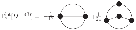
This section contains general information about the correlation functions of QCD in linear covariant gauges.222 In the literature, also the term Green’s function is used for a general correlation function, although mathematically only a propagator fulfills its definition. Both terms Green function and Green’s function are in use, the latter being correct from the historical linguistic viewpoint. Despite the fact that Green function corresponds to the prevalent style in modern English, Green’s function is predominantly used [39]. Their structures in color, Lorentz and Dirac spaces are described and their DSEs are given in untruncated form if not noted otherwise. In addition, for the three-point functions the equations of motion from a three-loop expansion of the three-particle irreducible (3PI) effective action are provided. Their forms are very similar to those of the corresponding DSEs, and they provide a useful alternative description for these vertices. Beyond the primitively divergent correlation functions, also details on the two-gluon-two-ghost and the four-ghost vertices are given, as they will be discussed in Sec. 4. For completeness, also the quark propagator and the quark-gluon vertex are included to provide a consistent description of full QCD. The derivations of the DSEs and equations of motion for the 3PI effective action will be described later in Sec. 3 where details like signs and numeric prefactors will also be explained. However, the equations are already given here to collect all the information about the description of correlation functions in one place. In later sections, subsets of these equations and their truncations will be discussed.
Since many different correlation functions will be treated, it will be convenient to use a common notation where the field content of the correlation functions is put in the upper index. denotes a gluon leg, a ghost/anti-ghost leg, and a quark/anti-quark leg. When the field content is clear because of the explicitly given Lorentz and color indices, the field indices may be omitted. The tree-level expression is denoted by a superscript . Tab. 1 contains an overview of all dressings and tensors introduced in the following.
Correlation functions with gluon legs can be split into transverse and longitudinal parts. To be precise, there are two ways of splitting a correlation function , see [40] for a detailed discussion:
| (28) |
and are defined as the parts that vanish when projecting longitudinally and transversely, respectively:
| (29) | ||||
| (30) |
is the transverse and the longitudinal projector. In general, and . is often called longitudinal, although it does not vanish when it is projected transversely. As a consequence, information about can be inferred using gauge techniques [41, 42, 43, 44] from longitudinal projections. This was applied in QCD for example in Refs. [45, 46, 47, 48, 49, 50, 51, 52]. On the other hand, the transversality of the gluon propagator in the Landau gauge leads to the closure of the parts of correlation functions [53] that survive when transverse projections are applied. Thus, is sufficient in this gauge. Keeping in mind these comments, we will now continue in agreement with the widespread use in the literature and call it transverse in the following. It should also be noted that the choice of a basis is subject to many considerations including technical and physical ones. For a discussion of the latter, see Ref. [40].
| Correlation function | Dressings | Tensors |
|---|---|---|
| Ghost propagator | 1 | |
| Gluon propagator | , | , |
| Quark two-point function | , | , |
| Ghost-gluon vertex | , | |
| Three-gluon vertex | ||
| Quark-gluon vertex | ||
| Four-gluon vertex | ||
| Two-ghost-two-gluon vertex | ||
| Four-ghost vertex |
2.2.1 Ghost propagator
The ghost field is a scalar field and hence its propagator has one dressing function only. The negative norm of the ghost field can be taken into account directly in the propagator via a minus sign:
| (31) |
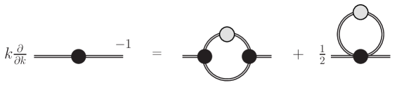
The tree-level corresponds to . The full DSE of the ghost propagator is given in Fig. 1.
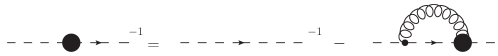

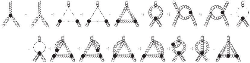
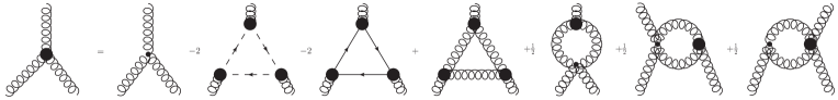
Here and in other figures, internal propagators are dressed, and thick blobs denote dressed vertices, wiggly lines gluons, dashed lines ghosts and continuous lines quarks.
2.2.2 Gluon propagator
The gluon propagator in linear covariant gauges is uniquely split into a transverse and a longitudinal part parametrized by two dressing functions:
| (32) | ||||
| (33) | ||||
| (34) |
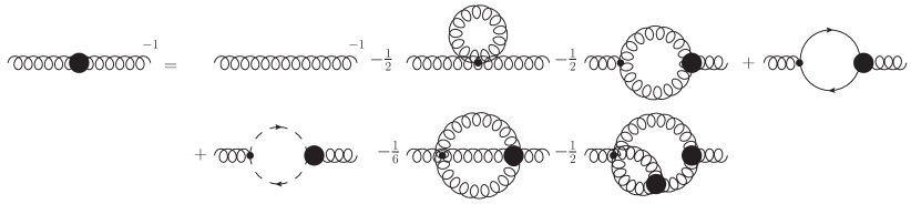
At the tree-level we have and . The Slavnov–Taylor identity (STI) of the gluon propagator fixes the longitudinal part to be equal to the gauge fixing parameter also beyond tree-level, . The full DSE of the gluon propagator is given in Fig. 1. It is equivalent to the corresponding equation of motion of the 4PI effective action [54].
2.2.3 Quark propagator
The quark propagator depends on two dressing functions which can be chosen in various ways. A typical parametrization starts from its inverse:
| (35) |
The tree-level is and with the bare quark mass. The propagator in terms of the two scalar functions and reads then
| (36) |
Two alternative parametrizations use the scalar and the vector dressing functions and , respectively, or the quark renormalization function and the quark mass function :
| (37) |
The full DSE of the quark propagator is given in Fig. 1.
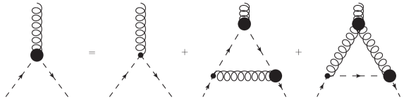
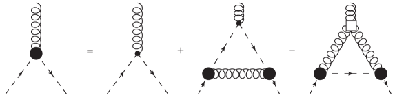
2.2.4 Ghost-gluon vertex
Three-point functions depend on two independent external momenta from which one constructs three variables. Possible sets are three squared momenta, two squared momenta and the angle between the two or even more complex combinations, see, e.g., [55]. In the following, typically the three external momenta are used as arguments. However, in plots for specific momentum configurations either three momentum squares or two momentum squares and the angle between the two corresponding momenta are used, e.g., or . The first two arguments refer to the gluon and anti-ghost momenta.
The full ghost-gluon vertex can be parametrized as
| (38) |
where the momentum arguments correspond to the order of the fields in the superscript. For a discussion of the color part see Sec. 2.2.5. All momenta are taken as incoming. The bare vertex has and . This parametrization of the vertex contains a part that is proportional to and thus vanishes upon contraction with the transverse projector. Contracting with a longitudinal projector, both tensors survive. Thus, it is elucidating to parametrize the vertex as follows where a clear separation into transverse and longitudinal parts is evident:
| (39) |
is the transverse projector.
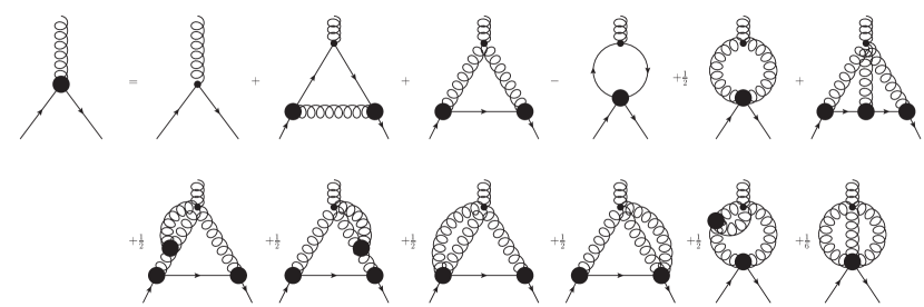
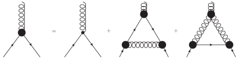
The ghost-gluon vertex has two different DSEs differing by the leg that is attached to the bare vertex. They are called - and -DSE. A third one, the -DSE, is due to the ghost–anti-ghost symmetry of the Landau gauge [20, 56] equivalent to the -DSE in this gauge. The two full DSEs and the equation of motion from the 3PI effective action in a three-loop expansion are depicted in Fig. 2. It should be noted that the - and -DSE are both exact, but truncations can have different effects on them. In contradistinction, the equation of motion from the 3PI effective action that is shown in Fig. 2 is obtained from a truncation of the effective action and thus not exact. Differences in the description of the ghost-gluon vertex due to using different truncations are discussed in detail in Secs. 4.2.5 and 4.3.3.

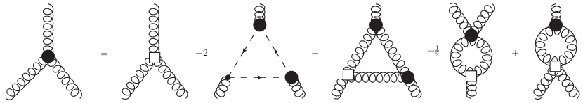
2.2.5 Three-gluon vertex
The three-gluon vertex has 14 tensors:
| (40) |
A possible color structure with the symmetric structure constant is ignored here, since it would be in conflict with the charge invariance of QCD [57, 58, 59]. In Sec. 4.2.5 it will be explained that in three-point DSEs can only arise from a decoupled part of the four-point functions.
The three-gluon vertex has 14 Lorentz tensors:
| (41) |
For the Landau gauge, the four-dimensional transverse sector is sufficient due to the closure of the corresponding parts of correlation functions [53]. The resulting transverse vertex can be written as:
| (42) |
The superscript to indicate that this is the transverse part will be suppressed whenever calculations in the Landau gauge are discussed. An explicit transverse basis can be constructed from the naive basis, viz., the set of all possible combinations of the two independent momenta and the metric tensor with three Lorentz indices. Upon transverse projection, six tensors survive, but only four are linearly independent. They can be chosen as
| (43) | ||||
| (44) | ||||
| (45) | ||||
| (46) |
As discussed around Eq. (28), this corresponds to the part of the vertex that survices when projected transversely, . Alternatively, considerations of the symmetry group underlying the Bose symmetry of the vertex can be used to construct a basis that has specific properties under permutations of the legs [55]. The bare vertex is given by
| (47) |
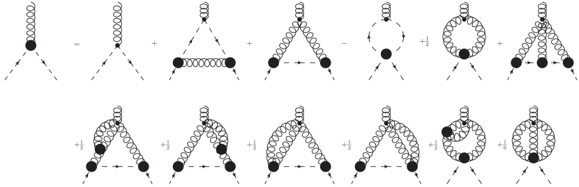
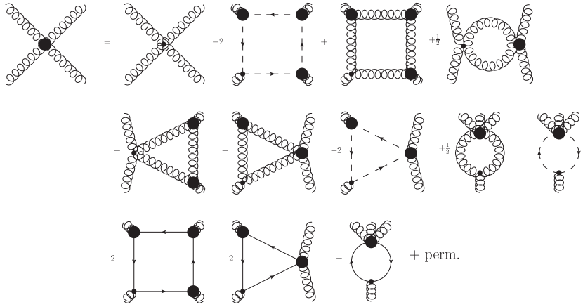
The full DSE of the three-gluon vertex and its equation of motion from the 3PI effective action in a three-loop expansion are depicted in Fig. 3.
2.2.6 Quark-gluon vertex
The full quark-gluon vertex has twelve tensors:
| (48) |
where is the generator of the gauge group. The transverse subspace is eight-dimensional:
| (49) |
Again, the superscript can be skipped in discussions of the Landau gauge. The tree-level vertex is
| (50) |
In the calculation of the quark-gluon vertex a good choice of the basis is particularly important. In particular, a bad choice can lead to numeric instabilities. Various versions have been used in the literature [60, 61, 48, 62, 63, 64, 65, 66, 67], among them the traditional Ball-Chiu basis [60] and variants thereof.
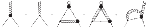
The diagrammatic structure of the quark-gluon vertex DSEs is the same as for the ghost-gluon vertex. Two of its three DSEs, which are all equivalent as long as they are not truncated, are depicted in full form in Fig. 4 as well as its equation of motion from the 3PI effective action in a three-loop expansion. The -DSE, which is not shown, is equivalent to the -DSE in the Landau gauge.
2.2.7 Four-gluon vertex
With four-point functions, which have three independent momenta, the size of the tensor space increases drastically. Writing down all tensors with four Lorentz indices constructed from the three independent momenta or the metric tensor leads to 138 tensors:
| (51) | |||||
| (52) | |||||
| (53) |
However, the basis is spanned by 136 tensors only, since some tensors are not linearly independent [40]. The transverse subspace has 41 tensors [40].
In addition, the color space is also more complicated. With four color indices, one can construct from the basis elements of the Kronecker delta and the symmetric and anti-symmetric structure constants and , respectively, the following 15 combinations:
| (54) | |||||
| (55) | |||||
| (56) | |||||
| (57) |
However, several identities relate tensors to each other [68]:
| (58) | ||||
| (59) | ||||
| and 2 permutations. |
The Jacobi identity is a combination of the permutations of Eq. (59). These identities reduce the number of independent tensors by six. Finally, for an additional identity reduces the final number of independent tensors to eight [68]:
| (60) |
For , there is no symmetric structure constant which reduces the number of tensors even further to three. In the following we will restrict ourselves to . Hence, for , one needs to generalize.
A full basis can be chosen as
| (61) |
Combining these tensors such that they have clear permutation symmetries would be advantageous. For now, however, we restrict ourselves to the permutations of with and with , as these symmetries are those relevant for the two-ghost-two-gluon vertex. The full symmetrization is discussed in Ref. [40]. The partially symmetric basis reads
| (62) |
The symmetry properties are summarized in Tab. 2.
| + | + | + | - | - | - | - | + | |
| + | + | + | - | - | + | - | - |
If the symmetric structure constant is neglected, the number of independent tensors reduces to five. Based on the relations in Eq. (59), one might expect that neglecting leads to problems with an incomplete basis. However, it was already noted in Ref. [69] that the set closes under DSE iterations if no symmetric color part from three-point functions is taken into account. Indeed, the sets and are orthogonal to each other for . The former set is called the reduced basis in the following. Furthermore, the second set only couples to the symmetric color part in the DSEs of three-point functions as discussed in Sec. 4.2.5.
The tree-level tensor of the four-gluon vertex is given by
| (63) |
The full transverse vertex can be written as
| (64) |
where the tensors are given by
| (65) |
with . A full list of the Lorentz tensors is not given here. For testing purposes, some specific dressing functions are used statically in Sec. 4.2.5, for example,
| (66) | ||||
| (67) |
Two other tensors, and , are constructed by transverse projection and orthonormalization of the set consisting of the tree-level tensor and these two tensors [70, 71]:
| (68) | |||
| (69) |
Four-point functions depend on three independent momenta. They can be chosen as follows:
| (70) |
The three radial variables , and and the three angles , and can then be taken to span the six-dimensional space for four-point functions.
2.2.8 Two-ghost-two-gluon vertex
The two-ghost-two-gluon vertex has two Lorentz indices what simplifies its treatment in Lorentz space considerably compared to the four-gluon vertex. In Lorentz space, the following basis is explicitly transverse and has clear (anti-)symmetry properties under the exchange of the gluon momenta:
| (71) |
Here, , the two gluon momenta are and and the anti-ghost/ghost momentum is . The full basis is constructed as the direct product in color and Lorentz space:
| (72) |
with . The vertex is then written as
| (73) |
Note that a factor of is put in front to account for the fact that the lowest diagrams are of this order, since there is no tree-level contribution as for the four-gluon vertex. In Sec. 4.2.5, it will be explained that dressings are sufficient corresponding to the reduced set of color tensors, because the other three color tensors do not couple to the reduced set or to three-point functions. As defined here, the dressing functions are dimensionful, because the vertex is dimensionless, but the Lorentz tensors are chosen as dimensionful.
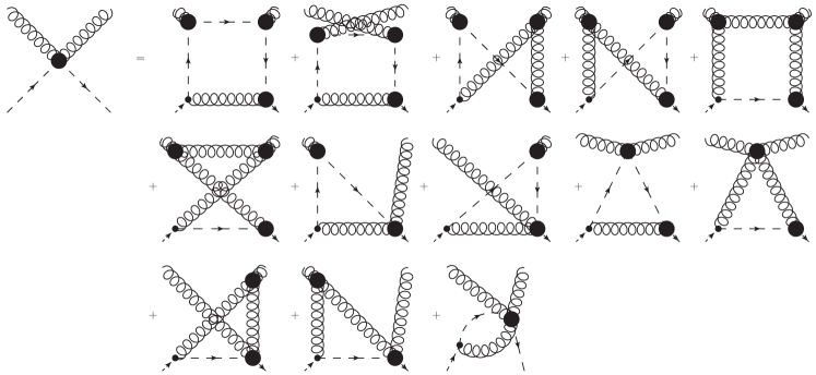
As typical for vertices of mixed types of fields, the two-ghost-two-gluon vertex has several DSEs. In analogy to the ghost-gluon vertex, they are called -DSE and -DSE based on which type of field is attached to the bare vertices. Due to the existence of a bare four-gluon vertex, the -DSE contains also two-loop terms, while the -DSE has a one-loop structure. An additional advantage of the -DSE is that in contrast to the -DSE, it does not contain a four-ghost vertex. The full -DSE is shown in Fig. 6.
2.2.9 Four-ghost vertex
The four-ghost vertex is a comparatively simple four-point function, because it is a scalar in Lorentz space. Thus, it features only eight tensors in total. The full vertex is written as
| (74) |
As for the two-ghost-two-gluon vertex, the reduced color basis is completely decoupled from the other three tensors and thus sufficient.
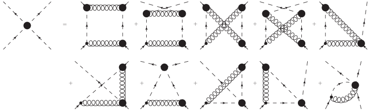
A full DSE of the vertex is shown in Fig. 7. Another one, where the bare vertex is attached to the anti-ghost leg, has the same structure.
3 Methods
Many methods are used to calculate correlation functions nonperturbatively. Sec. 3.1 contains details on different functional equations with a focus on equations of motion from PI effective actions and the functional renormalization group. The Hamiltonian approach is also sketched. Furthermore, an overview of available technical tools is given. The section concludes with a short comparative summary of functional methods. In Sec. 3.2, further methods are shortly discussed.
3.1 Functional equations
Functional equations relate correlation functions via integral, differential or integro–differential equations. They come in different variants, for example, as equations of motion of correlations functions or as equations expressing underlying symmetries. In the main part of this work only the correlations functions of QCD are considered, but functional methods are very general and can be used in many different fields of physics, ranging from condensed matter to quantum field theory to gravity. This section is kept general and describes the derivation of different functional equations. Before details on specific functional equations are given, some general definitions are provided.
In the following, the path integral formalism is used as it is the most natural way to deal with functional equations. To keep things general and to avoid cumbersome notation, a super-field is introduced where the index represents a field-type and all of its indices as well as position or momentum. Repeated indices are summed/integrated over. The action can then be represented as
| (75) |
For conventional reasons, minus signs were put in front of the interaction terms. The coefficients , and denote the bare two-, three and four-point functions and the statistical factors are chosen for convenience. Here, only three- and four-point functions are included, but it is straightforward to add higher terms.
The path integral is given by
| (76) |
where the sources were introduced as well as the generating functional of connected correlation functions, . The central object we are interested in is the effective action which is obtained as the Legendre transformation of :
| (77) |
The effective action depends on the averaged field in the presence of the external source :
| (78) |
The inverse relation is
| (79) |
The effective action can be expanded in -point functions , also called vertex functions, around the physical ground state, which is taken here as :
| (80) |
The are symmetry factors. The derivatives of the effective action are denoted as where the superscript is kept to indicate that the sources are not set to zero333The negative sign is a choice of convention. It counteracts the minus sign appearing from the derivative in Eq. (91b) below.:
| (81) | ||||
| (82) |
The coefficients in the vertex expansion correspond to
| (83) |
The two-point functions play a special role, since they are the inverse of the propagators . For non-zero sources the relation is
| (84) |
and the physical propagator is given by
| (85) |
It should be noted that Eq. (84) is a matrix relation in field space.
3.1.1 Dyson–Schwinger equations
Dyson-Schwinger equations are named after Julian Schwinger and Freeman Dyson who initiated the use of these equations [72, 73, 74]. Nowadays, they are most conveniently written as integral equations and derived in the path integral formalism. DSEs can be derived from the following total derivative:
| (86) |
This is the generating equation for the DSEs of full correlation functions. To switch to connected correlation functions, the generating functional is replaced by and the identity
| (87) |
is used. After multiplying with from the left, Eq. (86) becomes
| (88) |
Finally, we perform a Legendre transformation to obtain the generating equation for the DSEs of one-particle irreducible (1PI) correlation functions. In the transformation, the derivative with respect to the sources becomes
| (89) |
and we finally have
| (90) |
An example for this equation is shown Fig. 8. From Eq. (90), all DSEs of 1PI correlation functions are obtained by differentiating with respect to fields and then setting the fields to their physical values. In the course of such derivations, the following differentiation rules are required:
| (91a) | ||||
| (91b) | ||||
| (91c) | ||||
These rules are depicted in graphical form in Fig. 9.
An example for a two-point function, obtained by performing one derivative of Eq. (90) with respect to a field, is shown in Fig. 10. It is important to keep diagrams with external fields until the end. Only then the sources are set to zero and thus the external fields take their physical values. In the cases considered in this work, the expectation value of fields is always zero.
A special application of DSEs in gauge field theories is the combination of the pinch technique [75, 76, 77, 78] with the background field method [79, 80] which is referred to as PT-BFM [81, 82, 83, 84]. A special advantage of this approach in QCD is that individual subsets of diagrams in the gluon propagator equation are fully transverse [83]. It was successfully employed for the study of propagators, e.g., [81, 85, 86, 87, 88, 45, 89, 90, 91, 92], and three-point functions [91, 49, 51, 52, 93, 94].
3.1.2 Equations of motion from PI effective actions
The effective action is given by the Legendre transformation of where is the expectation value of the field variable. One can treat the propagator and the proper vertices on the same footing as the expectation value of the field by adding corresponding sources:
| (92) |
The are source terms for the propagator , defined in Eq. (85), and the vertices , defined in Eq. (83), where the superscript was added to denote the order of a vertex. With follows
| (93) | ||||
| (94) | ||||
| (95) |
is the third derivative of with respect to .
Performing additional Legendre transformations, the corresponding PI effective action is obtained:
| (96) |
From Eq. (96), one can show
| (97) |
For the last equation, was used. For vanishing sources this leads to the stationarity conditions
| (98) |
from which the equations of motion of correlations functions follow.
The effective action is called 2PI effective action as it contains only 2-particle irreducible diagrams [97], viz., it only contains diagrams which cannot be separated by cutting two lines. The 3PI effective action is obtained by performing an additional Legendre transformation with respect to three-point functions [98, 54]. It contains only 3-particle irreducible diagrams. Effective actions with Legendre transformations up to -point functions are called PI effective actions, although the property of -particle irreducibility does not hold any more for the 5PI effective action [54]. All effective actions are equivalent, viz.,
| (99) |
However, in PI effective actions with , propagators and vertices are not all treated on the same footing, because -point functions with are not dressed. Thus, only correlation functions up to legs are treated self-consistently.
For practical calculations, typically loop expansions of PI effective actions are considered. For a self-consistent expansion of an PI effective action at least an -loop expansion is necessary [98]. Higher PI effective actions are equivalent at the same expansion order:
| (100) | ||||
| (101) | ||||
| (102) |
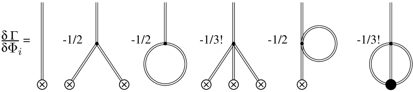
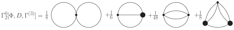
As an example, the three-loop expansion of the 3PI effective action of a scalar theory with cubic and quartic interactions is considered in the following. The generalization to QCD can be done diagrammatically following the usual rules, viz., by endowing the fields with the appropriate indices and the diagrams with closed loops of Grassmann fields with additional minus signs. Details for QCD can be found in Ref. [98]. For the derivation of the 3PI effective action, it is convenient to start with the 2PI effective action [97] and perform another Legendre transformation. The loop expansion of the 2PI effective action itself is derived using a loop expansion of the 1PI effective action [99]. The resulting expression is [98, 54]
| (103) |
is the field dependent inverse propagator defined as . contains bare vertices, whereas depends only on dressed quantities. They are given by
| (104) | ||||
| (105) |
Graphically, these expressions are depicted in Fig. 11.
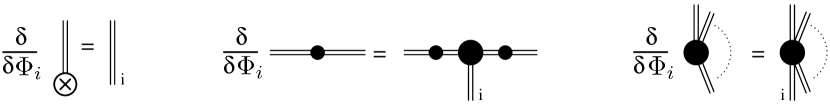
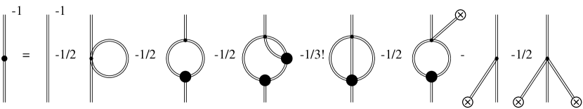
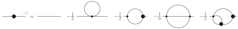
The equations of motion for the propagator and the vertex are derived from the stationarity conditions in Eq. (98). For the propagator one obtains
| (106) |
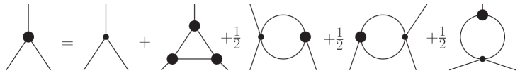
where is the bare propagator. Following through with the derivative one arrives at an expression that does not yet resemble the corresponding DSE. However, it can be rewritten using the equation for the vertex which is shown in Fig. 12. It is used to replace the vertex in the diagram with two dressed vertices. This insertion corrects the prefactors of the other diagrams and leads to the equation depicted in Fig. 13. The equation is identical to the DSE except for the four-point functions which are bare here. This is a direct consequence of using the 3PI effective action in which only the bare four-vertex appears.
3.1.3 Functional renormalization group
The functional renormalization group (FRG) is a versatile tool used in a wide range of fields including ultracold fermion gases, e.g., [100, 101, 102], supersymmetric models, e.g., [103, 104, 105, 106, 107], gravity, e.g., [108, 109, 110, 111, 112, 113, 114, 115, 116, 117, 118, 119], Higgs physics, e.g., [120, 121, 122, 123] and the phase diagram of QCD, e.g.,[124, 125, 126, 127, 128, 129, 130, 131, 132, 133, 134, 135, 136, 137]. This list is necessarily incomplete. For general reviews see Refs. [138, 139, 140, 124]. A short overview of the idea of the functional renormalization group is given in the following.
The central object in the FRG is the effective average action . It introduces an artificial momentum scale that allows to interpolate between the ultraviolet (UV) and the infrared (IR). In the limit , where is the UV cutoff of the theory, the effective average action corresponds to the bare action at the cutoff, . Lowering the scale , all quantum fluctuations above are integrated out successively. For , the full quantum effective action is recovered.
To introduce the scale , the action is modified by a regulator term:
| (107) |
The regulator function needs to possess the following properties: (1) It has to vanish for to obtain the standard effective action in this limit. (2) It has to diverge for so that the classical action is recovered in this limit. (3) For small momenta it must be proportional to , thus behaving like an effective mass acting as an IR cutoff for fluctuations with small momenta. (4) It has to vanish for large momenta so that it does not interfere with the high momentum behavior.
The effective average action is obtained via a modified Legendre transformation:
| (108) |
with
| (109) |
The dependence of the effective average action on the scale is described by a flow equation:
| (110) |
Here, and Eq. (109) was used to cancel the second and third terms in the first line. was decomposed as . is the connected propagator in presence of the sources at the regulator scale :
| (111) |
Its inverse is the two-point function but with an additional contribution from the regulator :
| (112) |
with
| (113) |
and
| (114) |
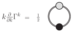
Hence, Eq. (3.1.3) can also be written as [141]
| (115) |
This equation is shown diagrammatically in Fig. 14. Solving the flow equation (115) corresponds to integrating out all fluctuations and going from a microscopic description, determined by the classical actions , to a macroscopic description. It should be noted that the trajectory in theory space but not the endpoint depends on the regulator function . However, this equation cannot be solved exactly and the necessary approximations lead to a regulator dependence of the endpoint.
From Eq. (115), flow equations for all correlation functions can be derived by applying derivatives with respect to fields. To this end, the following differentiation rules are required:
| (116a) | ||||
| (116b) | ||||
Again, the external sources are set to zero at the end and and correspond to the propagators and vertices of the theory for fixed . For Grassmann fields, the expected minus signs arise directly from their anticommutativity. As an example, consider the two-point function of a scalar theory. Two derivatives yield
| (117) |
The flow equation is obtained by setting the external source . The resulting integro-differential equation is depicted in Fig. 15.
As is clear from the flow equation of the effective average action, flow equations only contain one-loop diagrams. From a technical point of view, this is very convenient. At the same time, for an -point function all vertices up to order appear. For example, in QCD the flow equation for the quark propagator contains tadpole diagrams with quark-gluon, quark-quark and quark-ghost scattering kernels in addition to the diagram with the quark-gluon vertices. This is in marked contrast to the quark propagator DSEs which contains only a single loop diagram.
A technical advantage of the FRG is that renormalization is implemented automatically via the regulator function. It makes the integrals UV finite and thus no extrapolation of correlation functions in the UV is required as is often the case otherwise. Solving a flow equation requires to calculate the integrals at fixed scale and solve the differential equation in . This adds an additional layer of complexity. However, often flow equations are considered under approximations that allow certain simplifications.
3.1.4 Hamiltonian approach
The Hamiltonian approach is shortly discussed here as it has some similarities with other functional methods. In contrast to the other sections, here solely its application to Yang-Mills theory is discussed. It uses the canonical quantization in the Weyl gauge, viz., . The residual gauge freedom in form of time-independent gauge transformations is fixed to the Coulomb gauge, . Resolving Gauss’s law for the longitudinal part of the momentum operator leads to an extra term in the Hamiltonian, the so-called Coulomb Hamiltonian. The final Hamiltonian depends only on transverse gauge fields. The method was extended to Landau gauge in Ref. [142].
Correlation functions are calculated from the corresponding vacuum expectation values:
| (118) |
where is a polynomial of fields. The functional integral runs over all configurations in Coulomb gauge. is the vacuum wave functional and is the Faddeev-Popov determinant of Coulomb gauge with the Faddeev-Popov operator given by444In Sec. 2.1.2, the Faddeev-Popov determinant was called and the Faddeev-Popov operator . The notation with and is used in some literature on the Coulomb gauge.
| (119) |
The vacuum wave functional cannot be obtained exactly by solving a functional Schrödinger equation with the exception of dimensions [143]. Hence, one uses an ansatz. It is convenient to rewrite the square modulus of the vacuum wave functional as
| (120) |
The functional integral in Eq. (118) has then strong similarities with the standard path integral formulation. Indeed, one can interpret as an action and make the ansatz [144]
| (121) |
For , the integral is purely Gaussian [145, 146, 147]. The coefficients , and are variational kernels that have to be determined by minimization of the vacuum energy [144]. They are given explicitly in Sec. 5.3.
In analogy with the standard path integral, one can directly derive equations relating the different correlation functions from the identity
| (122) |
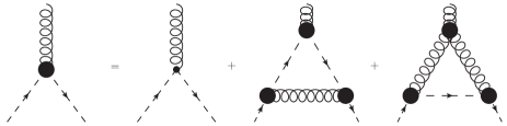
The truncated equation for the three-gluon vertex is shown in Fig. 16. For correlation functions involving ghost legs, one can also start from the inversion of the Faddeev-Popov operator given in Eq. (119), multiplies it with the appropriate number of gluon fields and takes the expectation value, see Ref. [148] for details. For the ghost-gluon vertex, for example, this leads as in the case of DSEs to two different equations. They are depicted in Fig. 17 in truncated form.
3.1.5 Technical tools
Part of the progress with functional equations in recent years was driven by new tools that were partially developed specifically for use with functional equations. The development of such tools became necessary with the systems of equations growing in size over the years. This was made possible by the increase in available computing power but also the improved conceptual understanding of the equations.
The calculation of a particular correlation function from a functional equation consists of two steps, the derivation of the equation and the actual process of solving it. For both steps dedicated programs exist which can also interface with each other. Advantageously, some of these programs were made publicly available and can be used by everyone. Of course, it depends on the specific problem if it is worth spending the time to learn how to use these programs. However, it should be clear that beyond a certain complexity of the problem automatizations become necessary.
The first publicly available program for the derivation of functional equations was DoDSE which is short for ’Derivation Of DSEs’ [149]. It is a Mathematica [150] package that can derive DSEs and represent them graphically. The output are DSEs in a symbolic form that does not refer to any specifics of the fields beyond their type. A single index contains all physical specifics like color, flavor or component similar to the notation used in Sec. 3.1.1. The commutation and anticommutation properties of the fields are taken into account as well. To use the abstract output in numeric calculations, it has first to be translated manually into the full algebraic form and then the contractions of indices have to be performed. Finally, these expressions have to be put into the numeric program.
While DoDSE represented the first step towards automatization and was capable of dealing with large systems of equations like arising for the maximally Abelian gauge (MAG) [151] or the Gribov-Zwanziger (GZ) action [152], the lack of output usable for numeric calculations constituted a major bottleneck. With the upgrade to version 2.0, a possibility was added to transform the symbolic output into algebraic form. To this end, the user needs to supply the corresponding Feynman rules. A tool to derive such rules from a given action was also added. The definition of Feynman rules also provides control over which parts of a correlation function to include. To contract the indices of the algebraic expression only rudimentary functions are provided like handling Kronecker deltas. The user is free to choose other available programs to perform such contractions of which there is a fair choice, e.g., FORM [153, 154, 155, 156, 157], FeynCalc [158, 159, 160], HEPMath [161] or TRACER [162]. The program FORM has a long tradition in high energy physics calculations as it is very efficient in corresponding calculations due to its specialization. However, using it requires learning the programming language. The Mathematica package FormTracer [163] makes the features of FORM relevant for functional calculations, viz., contractions of Lorentz, color and Dirac indices, directly available in Mathematica while still having a very flexible syntax.
Version 2.0 of DoDSE added the derivation of functional flow equations [164]. Hence the name was changed to DoFun, ’Derivation Of FUNctional equations’. The inclusion of flow equations expanded the applicability of DoFun to gravity [116] and effective QCD models including the Nambu–Jona-Lasinio (NJL) and quark-meson models [165, 166, 167, 168, 169, 170]. It was also used for QCD and Yang-Mills theory [171, 151, 152, 172, 173, 174, 175, 176, 177, 65, 178, 71, 179, 180, 181, 182, 183, 184, 185, 137, 186, 137, 67, 187, 188, 189, 190, 169, 191, 192, 24], the Thirring model [193] and for calculations of spectral functions in the model [194].
In version 3.0 [195], the workflow was made more flexible by implementing stricter rules for the definition of fields and the code was partially restructured for easier maintainance. In addition, the derivation of equations for composite operators was included and the code was put on a public GitHub repository, https://github.com/markusqh/DoFun. Bugfixes and updates are also made accessible via this webpage. At the time of writing, the current version number is 3.0.1. The documentation of DoFun is contained in Mathematica’s Documentation Center.
For solving functional equations numerically, a wide range of programs can be used, e.g., C, C++, Fortran, Python or Julia. Various packages can be used to deal with standard operations like integration or interpolation. Technical details on solving DSEs can be found, e.g., in Refs. [196, 197, 198, 199]. A framework for handling DSEs is provided by CrasyDSE [198] written in C++. The name is an acronym for ’Computation of RAther large SYstems of DSEs’. It does not rely on any particular packages to make it as autonomous as possible. Hence it can be deployed easily on different systems without worrying about dependencies. Naturally, this comes at the price of not being as fast as some dedicated packages. CrasyDSE consists of separate modules for integration, interpolation and handling DSEs which can be used independently from each other. A useful tool contained in CrasyDSE is a Mathematica package that provides the functionality to create kernel files from expressions in Mathematica. This can be used directly with the output of DoFun, but it works with general expressions.
FORM [153, 154, 155, 156, 157] was already mentioned as a tool for contracting indices. In addition, it provides an optimization routine [156, 157] that brings large expressions into a form that not only reduces their size but also speeds up their evaluation considerably. For large kernels as appearing, for example, for four-point functions [183, 188], such optimization routines are extremely helpful. Expressions can be passed on from Mathematica to FORM, optimized with it and then be read back in to export them to dedicated kernel files, e.g., with CrasyDSE. Alternatively, FormTracer also provides access to this FORM feature.
In summary, recent years have seen an increased use of automated tools for deriving and solving functional equations. Such tools are helpful not only to reduce errors and allow an efficient treatment, but given the size and complexity of modern truncations their use has become obligatory in many cases and their importance will most likely grow. It should also be noted that public availability and exposition of technical details increase the accessibility of the field and the trust in the results by researchers from other fields. Thus, any effort to make tools and programs public in the future is welcome.
3.1.6 Summary: Similarities and differences of functional approaches
All of the functional equations described above share some similarities. They can be represented with Feynman diagrams of dressed and, in some cases, bare quantities. The Feynman diagrams correspond to integrals, but also differential forms of the equations exist, e.g., [200].
An interesting difference lies in the role of bare quantities. While in DSEs every diagram contains one bare vertex, flow equations contain only dressed vertices. Thus, although some diagrams look very similar except for one bare/dressed vertex, there are also diagrams appearing only in one set of equations. In the equations of motion of PI effective actions, bare quantities appear either because the corresponding vertex has more than legs, or because a resummation takes place that leads to the same diagrams as for the 1PI effective action. In the Hamiltonian approach, some bare vertices are replaced by variational kernels which are determined separately by a variational principle. The variational kernels thus contain already more nonperturbative information than the standard bare vertices. Tab. 3 contains an overview of the differences between equations of motion and flow equations.
| DSEs | PI | FRG | |
|---|---|---|---|
| Effective action | |||
| Loops | fixed | loop expansion possible | 1 |
| Bare vertices | one per diagram | yes | none |
| Remarks | integrated RGEs | differential DSEs, | |
| regulator |
DSEs and equations of motion of PI effective actions are naturally very similar on the technical level, since DSEs are nothing else than the equations of motion of the 1PI effective action. Thus, the same techniques can be used to solve them. The equations of the Hamiltonian approach have a similar structure as well. However, the appearance of variational kernels instead of bare vertices requires to rethink the renormalization procedure, since variational kernels can have a different momentum structure than the bare vertices, see, e.g., Ref. [178]. Flow equations, finally, can be handled in a similar fashion for fixed renormalization group (RG) scale , but in addition the solution of the differential equation in is required. The appearance of the regulator has advantages as far as regularization is concerned. However, it also complicates real-time calculations by introducing additional poles [201].
3.2 Other methods
QCD correlation functions are studied with a range of methods. Their complementarities, e.g., analytic vs. numerical, continuous vs. discrete spacetime, are useful and sometimes lead to additional benefits. In this section, methods other than functional methods are shortly reviewed to sketch the landscape of approaches used for studying nonperturbative QCD.
3.2.1 Monte Carlo simulations on the lattice
Lattice QCD, viz., Monte Carlo simulations of QCD on a discretized spacetime [12], are very successful in describing many aspects of QCD e.g., [13, 14, 15, 17, 18, 16]. It relies on making spacetime discrete and finite by reducing it to a lattice on a four-dimensional torus. The quark fields live on the sites of the lattice and the gauge fields on the links. This formulation is very convenient from the conceptual point of view, because the UV regularization via the lattice spacing does not break gauge symmetry. In addition, physical quantities, viz., gauge independent quantities, can be calculated directly without fixing a gauge.
However, to make contact with other nonperturbative methods it is useful to fix the gauge nevertheless. Then, quantities like correlation functions of elementary fields can be calculated and directly compared. Unfortunately, the gauge fixing procedure is not unique due to the Gribov problem mentioned in Sec. 2.1.2. This directly affects lattice calculations as different algorithms to fix the gauge can be used. Based on the specific way to choose a gauge copy, ’different’ gauges can be defined which are equivalent on the perturbative level. For example, in case of the Landau gauge, choosing the first copy found is known as minimal Landau gauge and choosing the copy with the lowest norm of the gauge configuration as absolute Landau gauge. Many other choices are possible, see, e.g., [202, 203, 204, 205, 206, 207, 208, 209, 210, 211, 212, 213, 214, 215]. Averages over the full gauge orbits constitute also a valid choice [216, 217, 218, 219, 220, 221, 222, 223, 224, 225, 226, 227, 228], but this approach has not been realized yet with lattice methods. Results for correlations functions are available for propagators, e.g., [229, 230, 209, 211, 210, 231, 232, 233, 234, 235, 236, 237, 238, 239, 240, 241, 242, 243, 206, 244, 245, 246, 247, 248, 249, 250, 251, 252, 208, 253, 254, 255, 256, 257, 258, 259] and three-point functions [260, 261, 237, 262, 263, 233, 241, 264] in two, three and four dimensions at zero and nonvanishing temperatures.
These results are very useful for comparisons with the results from functional methods. However, care must be taken in such comparisons. In lattice studies questions of infinite volume and continuum limits are not always fully clarified. In addition, it is not clear which gauge fixing prescription on the lattice corresponds to which solution of functional equations. In some cases, the two approaches were also combined. For example, fits to gluon propagator results can be used as input in functional equations at nonvanishing temperatures [265, 266, 267, 268, 269, 270, 186, 271].
3.2.2 (Refined) Gribov-Zwanziger framework
As mentioned in Sec. 2.1.2, it is not possible to fix a gauge uniquely in the continuum. For example, many gauges can be implemented by introducing a delta functional of a gauge fixing functional or a Gaussian smearing of it together with the Jacobian, the Faddeev-Popov operator. However, this always leaves some remnant gauge copies. Gribov suggested a way to alleviate the situation [28] by restricting the integration in field configuration space on the gauge fixing hypersurface to a smaller region defined as the region where the Faddeev-Popov operator is positive. This region is nowadays known as first Gribov region, bounded by the Gribov horizon. At the boundary, the first eigenvalue of the Faddeev-Popov operator becomes zero and directly beyond the horizon the Faddeev-Popov determinant is negative. Where the second eigenvalue becomes negative and the determinant becomes positive again, the second Gribov horizon is crossed from the second to the third Gribov region. However, even if the restriction to the first Gribov region can be implemented, there are still gauge copies [272].
Formally, one can define a copy-free region called the fundamental modular region (FMR) [272]. It is contained within the first Gribov region and shares some of its boundary. Some of its boundary points are identified which makes the FMR a nonlocal and highly nontrivial object. It is not known how to fix the gauge to this region in the continuum. On the lattice, finding the absolute minimum is also not feasible, since this minimization problem is of the spin-glass type. However, one can approximate the search by taking the lowest minimum of the gauge fixing functional found in a (finite) sampling of the gauge orbit. This is known as the absolute Landau gauge.
For the Landau gauge, the first Gribov region is defined by
| (123) |
is the Faddeev-Popov operator which is related to the ghost propagator as
| (124) |
Gribov’s idea to restrict the integration in field configuration space to the region where is positive relied on parametrizing the ghost propagator as [28]
| (125) |
It can be shown that increases with decreasing . Thus, it is sufficient to demand . This relation is known as no-pole condition. The ghost-self-energy can be calculated as a series in the external field . In the path integral, the no-pole condition can be implemented via a Heaviside functional as
| (126) |
Using the saddle-point method, the integral over can be evaluated. then takes a certain value which is also known as Gribov parameter. It has the dimension of mass and must be calculated separately.
The generalization to all orders shows that one can add the so-called horizon condition to the Lagrangian density that implements the restriction to the first Gribov horizon [273]:
| (127) |
This expression can be localized by introducing four new fields forming a BRST quartet leading to the so-called Gribov-Zwanziger (GZ) action [274]. The resulting action has a gluon propagator that vanishes at tree-level [275]. The ghost dressing function at one-loop level is IR divergent [274, 202]. Among other things, the breaking of the standard BRST symmetry [276], the definition of a nonperturbative BRST transformation for this action [277, 278] or the construction of physical operators [279, 280, 281] were also investigated.
A generalization of the GZ action takes into account the existence of several condensates [282]. This is known as the refined Gribov-Zwanziger (RGZ) action. The form of the action depends on details of the considered condensates [282, 283, 284], but it is always chosen such that the gluon propagator at tree-level and the ghost dressing function at one-loop level are IR finite. The condensates are difficult to calculate dynamically. Thus, they are typically determined by fits to lattice data [239]. Such results can then be used in further calculations as input in analytic form. For example, glueball masses [285, 286, 287], the Polyakov loop [288] or the topological susceptibility [289] were calculated. The method, originating in Landau gauge, was extended also to the maximally Abelian gauge [290, 291, 292, 293, 294] and linear covariant gauges [295, 296, 297, 298].
3.2.3 Massive extensions of Yang-Mills theory
The fact that lattice simulations find a non-zero and finite value for the gluon propagator at zero momentum has motivated several model studies that contain a mass term for the gluon in the Lagrangian. This term is sometimes considered only on a phenomenological level, but there are also approaches with a physical motivation. The refined Gribov-Zwanziger framework, mentioned in Sec. 3.2.2, belongs to the latter class, ascribing the mass term to the existence of certain condensates arising from the restriction of the integration in the path integral to the first Gribov region.
Another approach that links a gluon mass to the Gribov problem leads to a massive extension of Yang-Mills theory [227, 228] in form of the Curci-Ferrari model [299]. In contrast to the refined Gribov-Zwanziger framework, which contains many nonperturbative condensates, only one additional parameter appears in form of a mass term for the gluon. With perturbative one-loop and two-loop calculations, an effective description of the nonperturbative regime is obtained, e.g., for two- [300, 301, 302, 303, 304] and three-point functions [305, 306]. Besides the coupling, the gluon mass is also a free parameter which can be fixed by fitting to lattice data. The analysis was also extended to two loops [307]. This model was also successfully applied to studies at nonzero temperatures and densities [308, 309, 310, 311, 312, 313, 314]. Other studies of massive extensions of Yang-Mills theory include [315, 316, 317, 318, 319, 320, 321, 322, 323, 324, 325, 326].
4 Correlation functions of Landau gauge Yang-Mills theory
The correlation functions of Yang-Mills theory have been studied with various methods ranging from phenomenological modeling to studies from first principles. While consensus has been reached in some questions, there are also some open issues pending further investigation. In particular, although several methods agree qualitatively and even quantitatively, there are still some subtle issues concerning details of gauge fixing.
In this section, the status of results from DSEs is reviewed. First, an overview of the Landau gauge is given. In the subsequent section, Yang-Mills theory in four dimensions is discussed. A particular focus lies on testing truncation dependences and clarifying some aspects which are important for a self-contained solution. The cases of three and two dimensional Yang-Mills theory are then investigated in Secs. 4.3 and 4.4, respectively. These theories are not only interesting by themselves, but they also allow insights on the general structure of functional equations and their truncations.
4.1 Landau gauge Yang-Mills theory
The Landau gauge is the gauge investigated best with functional methods. It is, technically speaking, more accessible than other gauges and was always a preferred gauge also for other methods. This allowed useful comparisons and complementary combinations of methods. Quite generally, it is also advantageous that the Landau gauge has the lowest number of ’terms’ possible. This refers, on the one hand, to the number of primitively divergent correlation functions. On the other hand, the physically relevant transverse correlation functions form a closed system [53] and the longitudinal ones do not need to be computed. Another set of functional equations, the STIs, constrains the longitudinal part only. Turning to other gauges, more dressings, for instance, the longitudinal ones in linear covariant gauges, or even more fields and interaction terms are needed. An example for the latter case is the maximally Abelian gauge where the diagonal and off-diagonal parts of all fields are treated separately thus doubling the field content.
It should also be mentioned that the Landau gauge has some interesting perturbative properties. Very often, Feynman gauge is used for perturbative calculations due to the simpler structure of the gluon propagator. However, when momentum subtraction (MOM) renormalization schemes are used, it turns out that the dependence on which vertex is used to define the coupling is weakest in the Landau gauge [327].
For studies of hadrons using bound state equations, the Landau gauge is also a standard choice. A vast list of calculations using effective interactions exists, see Refs. [21, 22] for recent reviews, but also results directly from calculated correlation functions were obtained, e.g., [66, 23].
Historically, the nonrenormalization of the ghost-gluon vertex played an important role in the investigation of the Landau gauge. The observation that his vertex is finite in the Landau gauge is attributed to Taylor and thus known as Taylor’s nonrenormalization theorem [328, 1]. Using an approximated STI, one can show that in the limit of the ghost momentum going to zero the vertex is bare. Variations for deriving this can be found, e.g., in [328, 1, 329, 330, 331, 332, 176]. Although it can only be shown for this special limit, it was often used as justification to employ a bare ghost-gluon vertex as ansatz. This was the entry point for many calculations of propagators. For the ghost propagator it is the only vertex that is needed and in the one-loop truncated gluon propagator only the three-gluon vertex remains to be specified. In dedicated calculations of the ghost-gluon vertex using lattice, functional and other methods, it was later found that the ghost-gluon vertex indeed shows only a quantitative deviation from a bare vertex [260, 333, 261, 237, 332, 175, 176, 305, 334, 335, 336, 51, 337, 24]. This explained the success of using this vertex ansatz. Investigations of other gauges, with the exception of the Coulomb gauge where the ghost-gluon vertex shows a similar behavior [338, 148, 178], are aggravated by the fact that corresponding simplifications are not known.
Another factor contributing to the widespread use of the Landau gauge in functional calculations is its accessibility with lattice methods which can thus be used for comparisons. The calculation of correlation functions with lattice methods has a long history itself. A breakthrough was achieved when finally lattice calculations were able to probe propagators also in the IR regime [246, 250, 247, 253]. Since then, the corresponding results in the midmomentum regime are often used as benchmarks for other methods. Propagators were studied heavily in two [230, 209, 211, 210, 231, 239, 232, 233, 241, 337], three [229, 234, 235, 230, 236, 231, 209, 237, 211, 210, 238, 239, 240, 232, 241, 337] and four dimensions [242, 243, 206, 244, 245, 246, 247, 248, 236, 249, 250, 251, 252, 208, 253, 254, 255, 256, 238, 239, 232, 257, 339, 233, 340, 241, 341, 342, 343, 337] and some results for vertices are available as well [260, 261, 237, 262, 263, 344, 264, 337]. Also for lattice calculations of correlation functions the Landau gauge is investigated best with only very limited results available beyond this gauge. However, some issues like gauge fixing ambiguities due to the Gribov problem are not fully settled yet and still actively investigated, e.g., [232, 213, 241, 337] and references therein.
An aspect of correlation functions of Yang-Mills theory that is most likely related to the unresolved Gribov issue is the existence of several solutions. Historically, the first calculation that solved the ghost and the gluon propagators together [345, 346] found a solution that is characterized by power laws of all dressing functions [330, 347, 348, 349, 350]. The gluon propagator was found to be IR vanishing and the ghost dressing function IR enhanced. This is in qualitative agreement with predictions in relation to the confinement scenario by Kugo and Ojima [34, 351] and in the GZ framework. The exponents of the corresponding power laws,
| (128) |
were shown to be related by [345, 346, 350]
| (129) |
The value obtained for was [352, 56, 175]. Lattice calculations at that time could not reach low enough momenta to confirm that. Only ten years later, first calculations on large enough lattices were made that showed a direct conflict with this behavior [246, 250, 247, 253]. What was found was an IR finite gluon propagator and an IR finite ghost dressing function. The solution of this type was named massive or decoupling solution and the earlier one scaling solution. Soon after these lattice results, solutions with this behavior were also found with other methods [282, 353, 354, 85, 53, 355]. However, the idea of the dynamic generation of a gluon mass goes back to the 80’s [75] and was investigated previously, for example, in Refs. [81, 356]. The current status is that both types of solutions can be obtained with functional and other continuum methods while on lattice only the decoupling solution is found. In particular, with functional equations it is possible to find an infinite number of decoupling solutions and the scaling solution corresponds to the endpoint with an infinite gluon mass [53]. If all these solutions are physically equivalent, they must necessarily lead to the same results for physical quantities. This was tested explicitly for scalar and pseudoscalar glueballs for which a range of different solutions was tested as input for their bound state equations, but no change in the spectrum was found [23]. It should be noted that only the scaling solution possesses an intact standard BRST symmetry [34] and this symmetry is not realized in lattice calculations [357, 217].
The fact that for the Landau gauge many results from lattice simulations exist also led to this gauge being a preferred gauge for many other methods. For example, models with a gluon mass term fix the value of this mass by fits to lattice results, e.g., [300, 301, 302, 319, 304]. Such approaches are discussed in Sec. 3.2.3. In the RGZ framework, originating in restricting the integration in the path integral to the first Gribov region [28, 275, 274], see Sec. 3.2.2, also fits to lattice data are often used, e.g., [239, 233], since a self-consistent determination of the corresponding quantities is difficult [284].
Beyond the vacuum, correlation functions have also been studied best in the Landau gauge. At vanishing density and nonzero temperature, lattice studies are less abundant than in the vacuum but still provide useful guidelines, e.g., [265, 358, 359, 360, 361, 362, 363]. At nonzero density there are currently no lattice results for correlation functions of QCD due to the complex action problem. However, results for the gauge group exist [364, 365, 366, 367]. With functional methods, studies range from using effective actions originally designed for hadron phenomenology, e.g., [368, 369, 370], to combinations with lattice methods, e.g., [266, 267, 371, 269, 270, 186, 192, 372, 373], to pure functional studies, e.g., [374, 131, 375, 376, 185, 137, 377, 191]. The most advanced pure functional studies calculated propagators [137, 376, 191] and even vertices [375, 137]. For a recent review on the DSE approach to the phase diagram of QCD see Ref. [378]. Also other methods rely on the Landau gauge for studies of the phase diagram of QCD, e.g., [311, 288, 313].
Finally, in the Landau gauge also results on the analytic structures of its propagators are available from different sources, e.g., [379, 380, 381, 382, 383, 384, 385, 386, 387, 388, 389, 390, 391, 392, 391, 393]. As far as the Yang-Mills propagators are concerned, the only direct functional calculation for complex momenta up to now was done in this gauge [382]. These results were used for solving bound state equations for the scalar and pseudoscalar glueballs [394]. For further calculations of glueballs using bound state equations see Refs. [395, 396, 397, 23]. The direct calculation of the analytic structures of propagators is possible with functional methods. However, there are technical obstacles related to calculating dressing functions for complex momenta [398, 201]. To overcome them, various techniques were developed [399, 400, 380, 381, 401, 402, 398, 383, 403], but they have not been applied to state-of-the-art truncations yet. More details are given in Sec. 4.2.4.
Since other gauges are investigated even less than the Landau gauge, one can consider the situation in the Landau gauge as the state of the art of gauge fixed nonperturbative studies of QCD. And despite the plethora of studies using the Landau gauge there is still much work to be done. There are some conceptual questions that need to be answered, for example, what role Gribov copies play and how different ways to fix the Landau gauge on the lattice are mirrored in functional equations. In recent years, studies with functional methods have made some big steps forward and provided interesting results on the question of the impact of truncations. Yet, when it comes to studies of the phase diagram, most results still rely on input from lattice results. Obtaining reliable results at nonvanishing density requires to repeat calculations in a more complicated setting and possibly extend the truncation setup. Such comprehensive studies should be the goal for the coming years.
4.2 Correlation functions from Dyson–Schwinger equations
Yang-Mills theory, being the limit of QCD with infinitely heavy quarks and describing the gluonic part of QCD, has been studied intensively with functional methods. For quite some time, it was assumed that the gluonic part of QCD constitutes the main obstacle to use functional methods for nonperturbative studies of QCD. The reason was that for a long time no quantitative results could be obtained and even the qualitative behavior in the IR was debated. The latter issue seems to be resolved nowadays, and the former is most likely close to a resolution. Results from the FRG give good reasons to believe that [184] and results from equations of motion presented here and in Ref. [24] also point in this direction. In this context it should be noted, though, that the matter sector of QCD turned out not to be as simple as expected for a long time. Recent studies indicate that in order to desert the successfully employed modeling in the quark sector and proceed to a self-contained solution, some unexpected subtleties still have to be resolved, see, e.g., [404, 61, 64, 63, 62, 65, 48, 66, 405, 406, 49, 67, 47, 94].
In this section several aspects important for a self-contained description from Dyson–Schwinger equations (DSEs) are discussed. Some of them have been an obvious item on the to-do list of DSE practitioners, for example, the inclusion of two-loop diagrams in the gluon propagator. Others, like the issue of quadratic divergences or the correct perturbative RG resummation, are only becoming important now, as their impact is only noticeable in new truncations. Secs. 4.2.1, 4.2.2 and 4.2.3 treat these points. The final section, Sec. 4.2.5, contains results for three- and four-point functions. In particular, the study of non-primitively divergent correlation functions in Sec. 4.2.5 is of interest with regard to the importance of higher correlation functions in functional equations.
4.2.1 Spurious divergences
QCD is a renormalizable quantum field theory. Employing the usual power counting, the superficial degree of divergence of correlation functions can be determined [407, 408]. The ghost and gluon propagators turn out to have a superficial degree of divergence of two (quadratic). All other correlation functions have a lower degree. However, the ghost two-point function must be proportional to the external momentum . Thus, any calculation automatically leads to a separation of this factor and the effective degree of divergence is zero (logarithmic) [407]. The gluon two-point function, on the other hand, has two tensors, and . For the latter, the same argument as for the ghost propagator applies, but for the former a quadratic divergence remains. Here, gauge symmetry comes to the rescue. It entails via an STI that the longitudinal part of the gluon propagator does not receive any quantum corrections and equals the tree-level. Only the transverse part of the propagator gets dressed where one can pull out a factor . And again the effective degree of divergence gets reduced to zero. Also for three-point functions the effective degrees of divergence are zero.
So in QCD all divergences are logarithmic. However, when calculating the gluon propagator explicitly, it turns out that it has quadratic divergences when a hard UV cutoff is employed. This also happens for other regularizations. Their common property is that they break gauge covariance. A notable exception to this is dimensional regularization [409, 410], which is widely employed for perturbative calculations. Unfortunately, its applicability to numeric calculations is difficult at best. It was tested for logarithmic divergences in quantum electrodynamics (QED) [411, 412] and for the Lippmann-Schwinger equation [413]. However, the regularization of power law divergences has not been attempted yet. In Ref. [413] it was noted that the employed technique relies on being able to directly take the limit . Power law divergences appear as poles in and the techniques must then be adapted accordingly.
Since dimensional regularization can (currently) not be applied to deal with the quadratic divergences of the gluon propagator, one has to find alternative ways. As it is numerically most convenient, one typically uses an invariant Euclidean cutoff . In analytic calculations, one can then discard the part of the result that contains the quadratic cutoff dependence. In numeric calculations, this cannot be done directly. In addition, the question of mixing between high and low momentum regimes arises, as we will see below.
Based on the observation that the gluon propagator corrections must be proportional to and the individual parts do not scale differently, Brown and Pennington argued that it would be sufficient to project onto , since the quadratic divergences only reside in the part proportional to [414]. This can be achieved with what has become known as the Brown-Pennington projector. It is a special case of the generalized projector
| (130) |
Acting on the two parts of the transverse tensor with this projector yields
| (131) | ||||
| (132) |
The Brown-Pennington projector corresponds to for which the first projection vanishes. While the quadratic divergences can be discarded with this projector, some new problems arise [56, 175]. First of all, when acting with on the right-hand side of the gluon propagator DSE, only , which corresponds to the transverse projector , ensures the absence of the longitudinal parts of the vertices. This would not be a problem if the longitudinal parts were known. However, we want to avoid calculating them. Furthermore, a projection with introduces a spurious parameter dependence [56]. To see this, the ghost-gluon vertex is written as (neglecting a part proportional to the gluon momentum for now)
| (133) |
and are parameters related by . A possible dressing of the vertex is taken to be one here. This approximation is sufficient in the UV and the arguments below would not be changed by a more general dressing. Th employed parametrization reflects that one can always shift contributions from the ghost to the anti-ghost legs due to the transversality of the Landau gauge:
| (134) |
Plugging this vertex into the gluon propagator DSE and projecting with , the kernel of the ghost loop becomes with and [179]
| (135) |
Appendix A.1 contains the full expressions for the DSE. One can see that only for the dependence on vanishes and for an undesired dependence on remains. Hence, only will be used in this work for calculations. Nevertheless, it will be kept explicitly in some analytic expressions.
The divergences in the gluon propagator DSE can be identified by analyzing the UV behavior of the equation. To this end, one approximates all dressing functions by their UV expressions and discards the external momentum in their arguments, since we are interested in the case . Then, all angle integrals can be performed. For the one-loop diagrams one obtains
| (136) |
and are the dressing functions and of the gluon and ghost propagators, respectively, in the UV. The dressing function of the three-gluon vertex in the UV is denoted by . The renormalization constants that appear are for the gluon field, for the ghost field, for the three-gluon vertex, for the ghost-gluon vertex and for the four-gluon vertex. The quadratically divergent part is proportional to .
To remove this part from the gluon propagator equation, various methods have been used in the past. Besides the Brown-Pennington projector, also modifications of the integrands [415, 416, 417, 374, 418, 419, 176], modifications of the vertices [53], fitting the momentum [380, 269] or the cutoff dependence [183], or additional counterterms [420, 421, 175, 188, 24] were used. In the combination of the pinch technique with the background field method, so-called seagull identities get rid of the quadratic divergences [86, 422]. Also in the functional renormalization group spurious divergences are introduced by the regulator. In practical calculations, it is overcome by fine-tuning the initial value of the gluon mass at the initial cutoff scale [184]. For a more detailed overview see Ref. [179].
For simple truncations, viz., using models for the vertices and only one-loop diagrams in the gluon propagator DSE, the subtraction terms can be calculated analytically [179]. In the UV, all dressings take their perturbative form. Here, we take for this the one-loop resummed expression discussed in detail in Sec. 4.2.2:
| (137) |
is the corresponding anomalous dimension and with . is any perturbative scale and is given by with the coupling. One can then perform the quadratically divergent integral in Eq. (4.2.1):
| (138) |
is the incomplete Gamma function. Its arguments are
| (139) |
where is the lower boundary of the integral. can be chosen equal to . This corresponds to the Landau pole of the employed parametrization of the perturbative dressings. Using an alternative parametrization, one can show that if is chosen as the lowest possible value, the results for both parametrizations agree [179]. For this choice of , the second term in Eq. (138) only cancels the imaginary part of the first part and leaves the real part untouched. Rewriting the incomplete Gamma functions into a convenient representation, the final subtraction coefficient is
| (140) |
is the anomalous dimension of the ghost propagator and is a coefficient that depends on the details of the vertex models. It should be noted that the result is not proportional to but to . The dependence on the cutoff is more intricate and completely encoded in the incomplete Gamma functions. This is a direct consequence of resummation in four-dimensional Yang-Mills theory. If we had used the leading tree-level contributions of the dressings, the result would be proportional to .
With this subtraction term, the quadratically divergent part can be subtracted from the gluon self-energy by adding . Assuming that all dressings behave like in Eq. (137), reads for the ghost and gluon loops of Eq. (4.2.1)
| (141) |
Note that RG improvement terms as discussed in Sec. 4.2.2 are not taken into account in this expression and still must be added appropriately. To test the precision of this method, the derivative with respect to the cutoff can be calculated which must agree with the original integrand. For an example calculation, this is shown in Fig. 18. It should be noted that a precise determination of the coefficient is important and that already tiny changes have an effect, see, for example, Fig. 36 below.
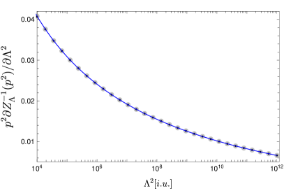
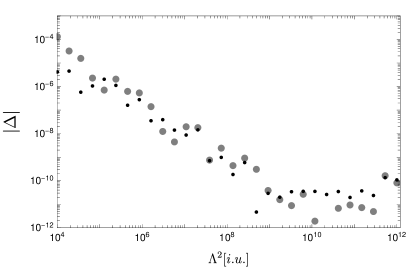
Unfortunately, this method of calculating the subtraction term is not feasible when dynamic vertices or two-loop diagrams are included. In that case, a convenient method is to introduce a mass counterterm for the gluon [421]. Although a mass term for the gluon is forbidden by gauge invariance of the Yang-Mills action, a counterterm can be introduced once a gauge is fixed [423]. One can then explicitly calculate this counterterm with a second renormalization condition. In practical calculations it is easiest to fix the gluon propagator at a low momentum value. Writing the gluon propagator DSE as
| (142) |
one can determine the renormalization constant by choosing a fixed value for :
| (143) |
is determined by demanding that the propagator has a fixed value at :
| (144) |
This method is employed for the two-loop calculation in Sec. 4.2.3. It should be noted that results can depend on this counterterm. However, for a large enough truncation, this dependence vanishes and the original number of relevant counterterms is restored [24].
4.2.2 Resummed perturbative behavior
In many studies of the QCD propagators using DSEs from the last 20 years, the one-loop resummed perturbative behavior is recovered. This means that the dressing functions behave at high momenta like a logarithm with a power known as anomalous dimension. The usual way to extract this behavior is solving the corresponding renormalization group equations which are based on the invariance of bare correlation functions under a change of the renormalization scale. A one-loop RG calculation leads to this anomalous running, whereas direct perturbative one-loop calculations yield only pure logarithms. However, the corresponding coefficients contain the anomalous dimensions. This is related to a general structure in perturbation theory that allows to predict certain aspects already from lower orders [423].
Unfortunately, this structure can be violated by truncations of DSEs. For example, it is in general not possible to solve a DSE self-consistently to a fixed order in perturbation theory. Self-consistency means here that the expression on the left-hand side of the equation is the same as on the right-hand side. A perturbative calculation lacks this consistency, as the right-hand side is calculated with a fixed input and the result is assigned to the left-hand side. A DSE, when solved self-consistently, has contributions up to infinite order. In the simplest case, a solution can be obtained by iteration. In this case, the left-hand side is repeatedly inserted on the right-hand side until it does not change any more. In every iteration step, a subset of higher order perturbative contributions is included. The best we can say perturbatively about the solution of a DSE is that it contains all contributions up to a certain order and some contributions beyond that.
Resummation in Dyson–Schwinger equations
So how can the anomalous running be obtained from a DSE? As the name resummed perturbative behavior suggests, its origin is in the resummation of certain diagrams. The renormalization group is a natural way to realize this resummation, but without exposing the individual contributions beyond one-loop. This is due to the aforementioned structure of perturbation theory. To perform resummation in DSEs, it is necessary to actually calculate these diagrams. The resulting series in the coupling constant can partially be resummed. To see how this works it is easiest to start from the other end. The one-loop resummed expression for a propagator dressing function reads
| (145) |
The anomalous dimension is denoted by . is the renormalization scale and the first coefficient of the -function. A series expansion yields
| (146) |
Thus, the resummation contains all terms which contain a logarithm of the same power as .
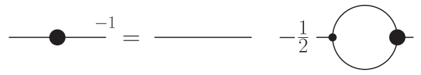
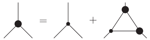
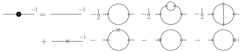
To illustrate how such terms are generated, we consider as an example a scalar theory in six dimensions with a cubic interaction:
| (147) |
The propagator DSE is shown in Fig. 19. The self-energy has one diagram at the perturbative one-loop level. At two-loop level, there are two diagrams, one from the one-loop vertex correction and one from the one-loop correction of the internal propagators. The corresponding diagrams are depicted in Fig. 20.
For simplicity, the following calculations are done in dimensional regularization considering dimensions and with . The calculation of the one-loop diagram yields [424]
| (148) |
Here and in the following, the numbers in parentheses in the superscript refer to the loop order. is the Euler-Mascheroni constant. The terms at order denoted by the dots will not be relevant in the following. We will also need the one-loop result for the vertex up to order :
| (149) |
Using the minimal subtraction (MS) scheme to fix the finite parts, the counterterms at one-loop level are:
| (150) | ||||
| (151) |
The two two-loop diagrams yield [424]
| (152) | ||||
| (153) |
is the propagator correction and the vertex correction depicted by the third and fourth diagrams, respectively, in the right-hand side in Fig. 20. As expected, terms proportional to appear in the finite parts. They will contribute at order to the resummation.
Renormalization beyond one-loop order requires that subdivergences are subtracted before the overall divergences are subtracted. At two-loop level, this is achieved by adding diagrams with appropriate counterterm insertions as shown in the second row of Fig. 20. For DSEs, the counterterms enter automatically at the right places and they do not need to be added explicitly, since one is working with renormalized quantities only. In this way, also overlapping divergences are automatically dealt with correctly in DSEs. As an example, consider the overlapping divergence arising from the second perturbative two-loop diagram shown in Fig. 20. It corresponds to a correction of the vertex and is also known as kite diagram. It contains two subdivergences which overlap and require separate counterterms. These are shown as the last two diagrams in Fig. 20. In the propagator DSE, Fig. 19, these counterterms enter differently: One is automatically included directly as the bare vertex comes with the renormalization constant of the vertex which is . The second one is contained in the dressed vertex. Its DSE contains as lowest order term also the renormalization constant and thus the appropriate counterterm.
The one-loop diagrams containing the one-loop counterterms are of order . The required integrals can be calculated from the expressions we already encountered, since they correspond to the one-loop diagram with additional momentum independent factors:
| (154) | ||||
| (155) |
The minus sign for stems from the fact that the counter term for the propagator at one-loop order is , because it is the inverse of the two-point function. The one-loop counterterms in the MS scheme contain only the terms of order . Thus, since we are here interested in the finite parts, we need the one-loop self-energy terms of order . The resulting expressions contain the following squared logarithms:
| (156) | ||||
| (157) |
Note that the disappearance of subdivergences, which is required for renormalizability, is reflected in the fact that all terms containing cancel out in the sum of all expressions.
Finally, if we sum all relevant terms from Fig. 20 and drop a factor of , we obtain
| (158) |
The prefactors were rearranged and expressed in terms of and . Eq. (4.2.2) corresponds to the first terms of the Taylor series of
| (159) |
This, however, is the one-loop solution to the renormalization group equation for the two-point function,
| (160) |
Thus, Eq. (159) corresponds to the one-loop resummed expression for the inverse propagator.
The resummed expressions thus contains all one-loop contributions and a subset of the higher terms. To realize the resummation in a DSE calculation, all contributions required for each order must be calculated. In particular, the renormalization constants have to be included correctly. In a one-loop truncation of the QCD propagator DSEs, already many terms of order and higher are contained via the nonperturbative propagators and possibly even the employed vertex models. However, in the gluon propagator DSE, the two-loop diagrams are required as they contain a sizable contribution to the second order. Higher terms can be included systematically, although this has been done only up to two-loop level up to now [188]. It turns out that this is sufficient and approximates the one-loop resummed behavior very well as discussed in Sec. 4.2.3. In particular, Fig. 22 in that section shows that the UV behavior of the propagator dressing functions recovers the pure perturbative one-loop resummed behavior quite well.
RG improvement in propagator equations: Yang-Mills propagators and other examples
In the remainder of this section it is discussed how the one-loop resummed behavior can be obtained in one-loop truncations. Most truncations do not contain two-loop terms for reasons of technical complexity. However, having the correct one-loop resummed perturbative behavior is advantageous and can be obtained by modifying the equations. This is done in many calculations and can be considered as part of the employed modeling of the missing parts. The modifications are derived by enforcing the self-consistency of a DSE in the perturbative regime. One possiblity to realize this is to interpolate between a given vertex model and an expression with the correct UV behavior [425]. However, since the necessary modification is part of the modeling anyway, once can include it directly in the vertex models. To see how this works, we consider the system of ghost and gluon propagator DSEs by following [415, 426, 176]. The dressing functions of the ghost and gluon propagators, and , respectively, can be parametrized as follows at the one-loop resummed level:
| (161a) | ||||
| (161b) | ||||
Here, is used as, for now, generic coefficient of the logarithm. Also the anomalous dimensions and are not specified yet. is a perturbative momentum scale.
The kernels of the propagator equations are given in Appendix A.1. We are interested in high external momenta . The integrals in the DSEs are dominated then by the region , where is a UV cutoff. In this regime, the momentum dependence of all dressing functions is dominated by the loop momentum . Hence, we approximate all dressing functions by ignoring the external momentum in their arguments, e.g., is replaced by , see also above Eq. (4.2.1). This allows calculating all three angle integrals analytically:
| (162) | ||||
| (163) |
Here, and and is a parameter from the projector kept for convenience. For the dressed ghost-gluon and three-gluon vertices only their tree-level structures, which dominate in the UV, were taken into account. They were dressed with the dressing functions and (depending only on the dominant scale), respectively, and the coupling was explicitly split off. Also the vertex dressings are taken to depend only on the large momentum scale with a form similar to Eqs. (161) with anomalous dimensions and . From counting the powers in in the integrals, the quadratic and logarithmic parts can be identified. The quadratic terms are discussed in Sec. 4.2.1. Here we are only interested in the logarithmic behavior and discard the other terms. Note that perturbatively the dependence cancels for the logarithmic terms between the ghost and the gluon loops. Plugging in the perturbative expressions for the dressings, the radial integral can also be performed:
| (164) | ||||
| (165) | ||||
| (166) |
The first terms in the brackets contain the cutoff dependence and are canceled by the renormalization constants. Of interest are the second terms. Self-consistency requires that the exponents of the logarithms are the same on the left- and right-hand sides. The dressings at the point are also discarded for the moment. Normally one discards these terms by choosing appropriate renormalization conditions [415]. We will see below that this is actually not necessary.
The ghost-gluon vertex is UV finite. Thus, its anomalous dimension is zero, , and was only kept for illustration purposes, as was the renormalization constant , which will be chosen as in the following. Matching the exponents in the ghost propagator DSE yields
| (167) |
which is a sum rule known from the perturbative renormalization group. The ghost-loop in the gluon propagator DSE leads to the same relation. If the exponents should match also for the gluon loop, the anomalous dimension of the three-gluon vertex must be . Plugging this in and setting , there are three equations (the exponents and the two coefficients in the two equations) from which one can determine , and as
| (168) | ||||
| (169) | ||||
| (170) |
The first coefficient of the Yang-Mills function, was used to highlight that corresponds to the expression used in Eq. (145).
Two things need to be emphasized with regard to the preceding calculation. First, the anomalous dimension of the three-gluon vertex is not . Second, taking into account also the dressings at , the solution does not look so simple anymore and depends on the relative sizes of , , , and . On the other hand, the approximation of taking only the loop momentum as argument of the dressing functions is not problematic. It actually turns out to work very well, as can be seen in the analysis of the quadratically divergent part which is extremely sensitive to even small deviations [179].
So how can one fix the analysis? The correct anomalous dimension of the three-gluon vertex is actually only half of the one above, viz., . One could thus think of replacing the dressed three-gluon vertex by the squared three-gluon vertex. This indeed leads to self-consistency also of the gluon propagator DSE. The same can even be done for the ghost-gluon vertex, as it does not change the exponents. It also cures the second problem by changing the coefficients as explained below.
It is known that from every vertex one can extract an expression for the running coupling [427, 330, 55], for example:
| (171a) | ||||
| (171b) | ||||
| (171c) | ||||
Here, . For a review on the QCD running coupling see Ref. [428]. The definitions above should be contrasted with the so-called MiniMOM [345, 429] or Taylor coupling [430]:
| (172) |
It agrees with for a bare ghost-gluon vertex. Its advantage is that the scale parameter can be determined from two-point functions alone. A range of studies exists for different numbers of quark families [431, 430, 432, 433, 434, 435, 436, 437, 438]. From the momentum dependent STIs it follows that the couplings (171) must agree in the perturbative regime. This entails
| (173) |
To make the coefficients of the two diagrams agree so that the STI can be used, we square the vertex dressings. then becomes
| (174) | ||||
| (175) |
The only term that is not accounted for is the renormalization constant of the three-gluon vertex, . The doubling of the vertex introduces an additional factor which modifies the behavior under changes of the renormalization scale. To maintain multiplicative renormalizability, we must counterbalance this change. By construction, the new term behaves under changes of the renormalization scale exactly as . Thus, we do not need it and discard it. There are two ways to do this: One can include a term in the vertex model or interpret the additional term as a momentum dependent renormalization constant [346]. The renormalization constant is related to the renormalization constants of the propagators via an STI:
| (176) |
The renormalization constants and run with the negative anomalous dimension, as can be seen from Eq. (4.2.2). Thus the ’anomalous dimension’ of is indeed . However, it runs with the cutoff, not with the momentum. Since the extra terms fix the RG running of the dressings, they are sometimes referred to as RG improvement terms [176].
It is interesting to compare these modifications with the flow equations of the functional RG. In these equations all vertices are dressed and no renormalization constants appear. Thus, dressing the bare vertices in DSEs seems like a natural choice. However, there is no one-to-one correspondence between a one-loop truncation with all vertices dressed and the complete equation.
While RG improvement terms are useful to get a self-consistent UV behavior, they also introduce problems, because the connection to the nonperturbative regime is not clear. There are various ways to continue the UV running to the nonperturbative regime and unfortunately results depend quantitatively on this choice. For the propagators, this was explicitly studied in [179]. Fig. 21 shows an example where two different versions of RG improvement terms were used. One version uses
| (177) |
where and are determined such that the anomalous dimension of the expression corresponds to the one of the three-gluon vertex. The remaining parameter is fixed such that the vertex becomes IR finite. For the scaling solution one obtains then and and for a decoupling solution and . This vertex model leads to the correct logarithmic running, but in the coefficients the factors of and do not combine as they should. However, it turns out that the inconsistency between the ghost and the gluon loops is not problematic in practical calculations, probably due to the fact that the gluon loop is perturbatively much larger then the ghost loop.
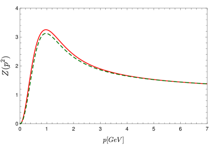
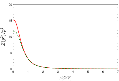
A second variant reads
| (178) |
It is motivated by the STI Eq. (176) and thus the factors of and combine as they should. The employed propagator dressings have the perturbative form with the Landau pole regularized:
| (179) | |||
| (180) |
with
| (181) |
Fig. 21 shows the influence of the choice of the RG improvement term. It is large enough that this effect has to be taken into account in modern truncations. For vertices such RG improvement terms were used in the past [177, 55, 71] as well. For the three-gluon vertex it was found that the RG improvement terms have a sizable impact also on the nonperturbative regime [55].
The usage of RG improvement terms works also in other cases. Let me illustrate this with the previous example of theory in six dimensions. The propagator dressing function behaves asymptotically as
| (182) |
We calculated in Sec. 4.2.2 that and with . The DSE of the propagator has the form depicted in Fig. 19:
| (183) |
is the field renormalization constant. The integral of the self-energy reads
| (184) |
The coupling was explicitly pulled out from the dressed three-point function. For the propagators we use now Eq. (182) and for the dressed three-point function we use a perturbative model that contains an RG improvement term and discards the renormalization constant in the self-energy:
| (185) |
is given by and the anomalous dimension of the vertex is . For large loop momenta we approximate the arguments of the dressing functions by their dominant part and obtain
| (186) |
Four angle integrals can be performed trivially: The fifth one can be done analytically as well, but the cases and have to be distinguished. We are only interested in the former case:
| (187) |
In the second step only the logarithmically divergent part was kept. The renormalization constant is determined by the expression depending on the cutoff . The second part must match the inverse dressing function on the left-hand side. From the exponents we obtain
| (188) |
Matching the coefficients yields
| (189) |
from which we infer
| (190) |
with the running coupling . In the Yang-Mills case the anomalous dimension could be calculated, because we used . Here, we also need some external information and took the anomalous dimension from the one-loop coefficient in Eq. (4.2.2).
Similar mechanisms to obtain the one-loop resummed behavior have also been employed in the quark sector. A version that is very close to the one explained above employs for the quark-gluon vertex a model that runs like the ghost dressing function squared. As in the previous examples, the self-consistency of the quark propagator equation using this ansatz can be shown by counting the powers of the logarithms. For simplicity we consider only the chiral case. The loop diagram contains a gluon propagator (anomalous dimension ), a quark propagator () and a quark-gluon vertex (). The integration leads to another power of the logarithm so that one ends up with as exponent of the logarithm on the right hand side. Since the anomalous dimension of the quark propagator wave function renormalization is zero, one can see that , where is the anomalous dimension of the ghost propagator, leads to the same relation as in the Yang-Mills sector: . The case where the anomalous dimensions of the integrand add up to as here is actually not well behaved, but a more detailed analysis, including also the quark mass function, shows that the general statements made here hold [439, 426]. The true anomalous dimension of the quark-gluon vertex, however, is . Again we see that an effective UV dressing of the bare vertex is necessary to enforce perturbative self-consistency at the one-loop level. In practical calculations of the quark propagator DSE, the modification of the anomalous dimension is realized, for example, by introducing an additional ghost dressing function in the model for the quark-gluon vertex, e.g., [439, 426, 45], or by directly changing the anomalous dimension from to [440]. The latter option was often used for calculations at nonvanishing temperatures and/or densities, e.g., [266, 267, 268, 269, 270, 441, 186, 271, 442, 192].
An alternative version to fix the one-loop resummed behavior was already used much earlier in form of the Maris-Tandy interaction. It also has a term that repairs the UV behavior at one-loop level [443, 444]. This interaction replaces the gluon propagator and the quark-gluon vertex dressing functions. The UV term of the interaction reads
| (191) |
At high momenta it behaves as
| (192) |
However, the combination of gluon propagator and quark-gluon vertex should run with the exponent . Again we see that a missing was added. With this interaction, the integrand has the same asymptotic behavior as in the previous case and the anomalous dimension of the quark wave function vanishes. Although this approach can be employed also at nonvanishing temperature [445], the UV part is typically ignored in such studies.
4.2.3 Two-loop diagrams in the gluon propagator DSE
The DSEs of QCD are two-loop exact, viz., only one- and two-loop diagrams appear.555The reason lies in the structure of the bare action of QCD that has only three- and four-point interactions. Higher interactions would lead to higher loop diagrams. At fixed order of perturbation theory, the hierarchy of diagrams is clear. For example, in the gluon propagator DSE the contributions at order stem from the explicit two-loop diagrams and the one-loop corrections of the propagators and vertices in the one-loop diagrams. However, as discussed in Sec. 4.2.2, they contribute to the one-loop resummed perturbative behavior. Here, it should only be noted that (some) two-loop diagrams are required to obtain the one-loop resummed perturbative behavior. In any case, in the perturbative regime there is a clear hierarchy of diagrams and one-loop diagrams are more important than two-loop diagrams. In the non-perturbative regime, on the other hand, the role of two-loop terms is a priori unclear, since no obvious ordering scheme exists. Hence, two-loop diagrams can become quantitatively more important than one-loop diagrams.
Unfortunately, two-loop diagrams are conceptually and numerically more difficult to calculate and corresponding studies are scarce. In DSEs they come in two types called sunset and squint diagrams, see Appendix B. Analytically, the importance of two-loop diagrams in the non-perturbative regime was analyzed for the scaling type of solutions in the Landau gauge [347, 348, 355, 350, 152, 446] and the maximally Abelian gauge (MAG) [447, 151, 448, 449]. Such analyses were made possible by the combination of the functional RG and DSEs as initially introduced in [347] or under the assumption of a convergent skeleton expansion [348, 355]. A general structure, which was worked out in Ref. [151, 448], emerges that explains why in the Landau gauge diagrams with the highest number of ghost propagators are dominant in the IR. This holds provided no cancellations appear, which, at least at the level of the propagator equations, would be very difficult to realize in this specific case. The corresponding analysis can also be applied to the Gribov-Zwanziger action [152]. Due to the mixing of fields at the two-point level the algebraic analysis yields four possible solutions at first, two of which could be discarded right away [152]. A third one was discarded later numerically [446], leaving as only solution the one which is equivalent to the solution from the Faddeev-Popov action.
The MAG constitutes a nice example where the hierarchy of diagrams is inverted in the IR. A scaling analysis revealed that certain sunset diagrams yield the dominant contributions in the IR with the corresponding squint diagrams possibly contributing as well [151]. The generalized method developed in Ref. [151] to determine the hierarchy of diagrams at low momenta was necessary to find this solution, since previously typically only the one-loop diagrams had been taken into account. More details on the MAG can be found in Sec. 5.2.
Numerical studies of two-loop diagrams were initially limited by the available computing power. A first inclusion via approximating one of the two loops was realized in [450]. Full numerical calculations were done later [451, 452, 453, 421, 183, 188, 24]. In the Landau gauge, an early finding was that the sunset diagram leads only to a very small change [451]. The squint diagram, on the other hand, has a larger impact as was shown in the case of four [452, 421] and three dimensions [183]. In Ref. [421], models for the vertices were used and their couplings were fitted to match lattice results of the propagators. In the latter case of Ref. [183], dynamically calculated vertices were employed that agree well with available lattice results. A solution in four dimensions with partially coupled vertices was obtained in [188] and the full system of primitively divergent correlation functions was solved in Ref. [24].
The analysis of two-loop diagrams is aggravated by the fact that analytic expressions are more difficult to obtain. A calculation using power laws for all the dressing functions as required for scaling type solutions can be realized using the negative dimension integration method (NDIM) [454, 455, 456, 457]. The case of two-loop diagrams is treated, e.g., in Ref. [458]. For the specific case of massless propagators and including a tensorial structure it was explicitly worked out in Ref. [448]. As in one-loop diagrams, spurious divergences appear in the two-loop diagrams which are best exposed when using a hard UV cutoff. However, in most perturbative studies, dimensional regularization is employed which cannot be used to identify these divergent terms. The sunset diagram was worked out for a UV cutoff in [451, 453]. The general method, which can also be applied to the squint diagram, is described in Appendix B. The corresponding results are discussed below. A numeric solution for the gluon propagator concludes the discussion of two-loop diagrams.
Analytic calculation of two-loop diagrams in the gluon propagator Dyson–Schwinger equation
The two-loop diagrams of the gluon propagator DSE, see Fig. 1, can be calculated analytically in the perturbative regime. The involved part are the angle integrations. With the method described in Appendix B, one can derive the following expressions for the squint and sunset integrals. Only the tree-level structure of the vertices is taken into account and all dressing functions have been set to one, so these are the perturbative results of leading order:
| (193) | ||||
| (194) |
The projector from Eq. (130) was used. with the being the loop momenta. The quadratic divergences can be identified as the terms proportional to as in the one-loop case. The remaining radial integrals can be done directly:
| (195) | ||||
| (196) |
Of direct relevance is the squared logarithm in the result for the squint diagram which is important for the resummation of logarithms. The sunset diagram does not yield such a term and thus does not contribute to the perturbative one-loop resummation at two-loop order.
Two-loop complete calculation of the Yang-Mills propagators
Being able to solve the two-loop diagrams in the gluon propagator DSE, one can solve the untruncated system of propagator DSEs of Yang-Mills theory. The vertices still need to be specified. For the ghost-gluon vertex, a bare vertex should be sufficient. However, since it is not problematic and actually advantageous for using the obtained propagator solutions as input for the vertex equations in Sec. 4.2.5, the ghost-gluon vertex will be included in a one-configuration approximation, see Sec. 4.2.5 for details. The four-gluon vertex is taken as bare. This vertex appears here only in the sunset diagram, which, however, is quantitatively not as important as the squint diagram. For the three-gluon vertex only the tree-level is dressed with the model function
| (197) |
is given by . This is a simple model with the correct UV behavior. The reason for choosing the structure is motivated by the UV analysis of the propagator DSEs, see Sec. 4.2.2. However, since this term is IR divergent, a damping function is added to tame it in the IR. The damping scale is chosen as . Note that neglecting non-tree-level dressings should be irrelevant for the perturbative resummation, since such dressings decay with a power law and thus do not yield terms proportional to .
One comment needs to be made about the tadpole diagram. Its role was scrutinized in Ref. [179]. While a small quantitative impact could not be excluded, it is clear that it behaves like a constant over . Thus, in most variants to subtract quadratic divergences it will be absorbed directly without any possibility to influence the results [179]. This is also the case for the method employed here where a second renormalization condition for the gluon propagator is used, . Any tadpole contribution will be absorbed in this condition and the tadpole is thus discarded.
The employed renormalization scheme is the MiniMOM scheme [346, 429], viz. the propagators are renormalized with a momentum subtraction. The specific renormalization conditions are for the ghost and , with , for the gluon. The momentum subtraction scheme entails that the renormalization constants of the ghost and the gluon propagators, and , respectively, are fixed implicitly and only once a solution is obtained, they can be calculated exactly. However, the renormalization constants of the three- and four-gluon vertices, and , respectively, are required as prefactors of the gluon loop and the two-loop diagrams. They are obtained from the corresponding STIs:
| (198) |
As a starting point, the solution of a one-loop truncated system of propagators is used. This gives access to values for and which are reasonable close to their final values so that the system can be solved with fixed values for and . From the solution, their new values are calculated and the system is solved again. This meta iteration process is continued until and do not change anymore. In these calculations, the value for the renormalized coupling was chosen as , since it is advantageous for the convergence of the resummed series to have a small value. However, must be large enough that the scale is inside the considered momentum region.
The results for the propagators are shown in Fig. 22. The two most important consequences of including the two-loop diagrams concern the UV behavior of the propagators and the quantitative changes in the midmomentum regime. A comparison of the obtained dressing functions with the analytic expression for the resummed one-loop behavior is also shown in Fig. 22. The plot shows that the solutions respect the expected behavior. It should be stressed, though, that only up to order all contributions are included. Beyond that, many contributions are included, for example, nested propagator self-energy insertions. Missing contributions are, for instance, contributions of order from the ghost-gluon vertex. Nevertheless, the agreement is quite good and is sufficient for practical purposes.
As expected, the inclusion of two-loop diagrams has an impact on the midmomentum regime. The more sizable contribution comes from the squint diagram, whereas the sunset diagram is relatively small. This can be tested by discarding the latter. The dressing functions do not change much then.
The present calculation still depends on models for the three- and four-gluon vertex. For a future complete analysis, full expressions for these vertices need to be used including non-tree-level dressings. The status of corresponding calculations of vertices is discussed in Sec. 4.2.5.
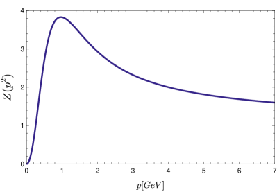
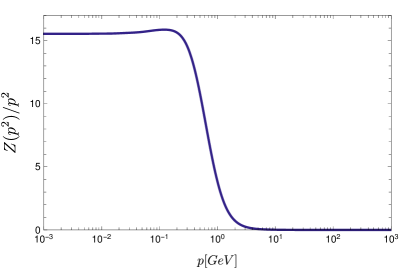
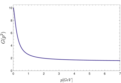
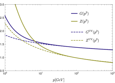
4.2.4 Analytic structure of the gluon propagator
The analytic structure of the gluon propagator is of interest for several reasons. In bound state equations the correlation functions of the constituent particles are accessed at complex values of the momenta, see, e.g., [20, 21, 22, 199]. Futhermore, the spectral function of a particle provides information about its spectrum. And finally, real-time quantities like transport coefficients require knowledge of the real-time properties of particles.
Functional equations are typically solved after a Wick rotation to Euclidean metric is performed, viz., the time coordinate is rotated to the imaginary axis as , where the subscript indicates now Euclidean time. In momentum space, this corresponds to . This entails . Calculations are then performed for real where no poles or branch cuts exist.
To undo the Wick rotation, Euclidean results need to be continued analytically to . This is an ill-posed inverse problem and always requires some form of bias. Possible reconstruction methods are, for example, the maximum entropy method [459, 460, 461, 462, 463, 464, 134, 465, 136, 466, 467, 468, 469], fits motivated by analytic results or phenomenology [470, 471, 472, 390], Padé approximants [473], the Schlessinger point method [474, 475], the Tikonov regularization [384], or the Backus-Gilbert method [470].
Alternatively, it is possible to solve the equations for complex momenta. However, this complicates any calculations considerably as care has to be taken which regions of the complex plane are probed in the integration. Poles or branch cuts constitute obstructions that have to be avoided. Methods suitable for this task include the shell method [399, 400], the Cauchy contour method [380, 400, 381], and others [383]. A very flexible method is based on contour deformation. Unfortunately, it is also very intricate and was thus not used extensively up to now. It was already successfully applied in QED [399], QCD [379, 382, 476] and for the scalar glueball propagator in the Born approximation [402]. The challenge is to deform the contour of the radial integration in such that any non-analyticities in the complex plane are avoided. Such non-analyticities can also be created by the angle integration [399, 379, 398]. For massless particles the contour deformation can be done along rays starting at the origin, see Ref. [477] for details. This ensures that the branch cut created by the angle integration is avoided via the only possible point , where is the complex external momentum. The integration path can then be continued outside the branch cut to the UV cutoff.
The analytic structure of a propagator is directly reflected in the spectral function. In general, one expects a branch cut for time-like momenta starting at a threshold value and possibly poles.666The possible existence of a term proportional to the Dirac delta functional is discussed in Refs. [388, 389, 392]. As a direct consequence of Cauchy’s integral formula the propagator can then be written as
| (199) |
where the sum is over the potential pole contributions with residues and masses which are either real with or complex. If there is only a real pole at , this expression can be rewritten as
| (200) |
with
| (201) |
and for . Eq. (200) has the form of a Stieltjes representation for the propagator [478, 479]. The inversion operation is formally known but includes infinitely many derivatives [478, 479, 480]. The difficulties in inverting this expression also become obvious when rewriting it as a double Laplace transform:
| (202) |
Eq. (200) has a physical interpretation as a sum of free propagators with density . This is called Källén-Lehmann spectral representation. It requires to be nonnegative so that the field is part of the physical state space of the theory. This is not necessarily the case for gauge theories, but Eq. (200) can be used even if contains negative contributions. Turning the argument around, negative norm contributions mean that the particle cannot describe an asymptotic phyiscal particle and is thus confined. This is a sufficient but not a necessary condition for confinement. Mathematically, it is encoded in the axiom of reflection positivity for Euclidean quantum field theory as formulated by Osterwalder and Schrader [481, 482]. It boils down to calculating the Schwinger function defined as the time Fourier transformation of the momentum space propagator for vanishing spatial momentum:
| (203) |
If the propagator can be written as in Eq. (200), this is the Laplace transform of the spectral density:
| (204) |
Clearly, if one can show that is negative somewhere, then must also contain negative contributions. If the propagator vanishes at zero momentum, as it does for a solution of the scaling type, positivity violation is obvious from
| (205) |
From the derivative of Eq. (200) with respect to , one can infer that a non-monotonous propagator also violates positivity. Such a behavior is seen in lattice and functional results in three dimensions, e.g., [258, 259, 233, 183, 189]. In four dimensions, the peak in the gluon propagator is only very small and not yet confirmed with lattice calculations. Functional methods, on the other hand, find such a peak, e.g., [53, 91, 184, 67, 188, 24] so that one can conclude without explicit calculation of the Schwinger function that positivity is violated also for decoupling type solutions. The existence of a maximum also has consequences for the spectral dimension of the gluon propagator, which is the dimension felt by the propagator. If the propagator has a maximum, it is reduced from four to one [483].
The Schwinger function can be calculated from Euclidean data alone and thus provides an easy means of testing for positivity violation. For the gluon propagator, the positivity violation in the Schwinger function was explicitly calculated with lattice and functional methods, e.g., [346, 379, 484, 485, 486, 53, 232, 335, 24]. The Schwinger function of the gluon propagator from Fig. 22 is shown in Fig. 23. Positivity violation is observed at a typical scale of about . For quarks, on the other hand, positivity violation is more subtle. In particular, it depends on the employed quark-gluon interaction and also the quark masses, see, for example, Refs. [379, 378].
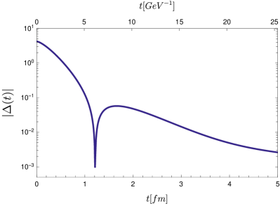
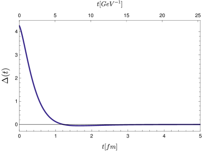
4.2.5 Vertices of Yang-Mills theory
In this section, results for the primitively divergent vertices of Yang-Mills theory, viz., the ghost-gluon, three-gluon and four-gluon vertices, as well as for two non-primitively divergent vertices, the two-ghost-two-gluon and four-ghost vertices, are discussed.
Ghost-gluon vertex
Three-point functions have for a long time only been modeled. This worked quite well for the ghost-gluon vertex, because using a bare vertex is close enough to the correct vertex that it is sufficient for many calculations. Only once quantitative precision is required, its quantum corrections need to be added. First semi-perturbative calculations using fits for the propagators recovered the qualitative behavior of the vertex actually quite well [333]. Later dynamical calculations only showed some quantitative changes [176, 334]. The full momentum dependence of the vertex is known up to two loops [487]. Further pertubative calculations can be found, for example, in Refs. [488, 489, 490, 491, 492, 493].
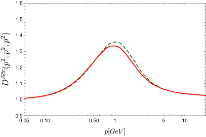
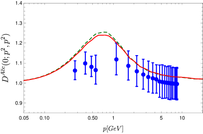
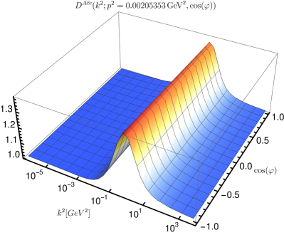
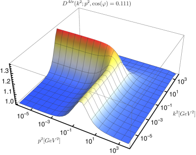
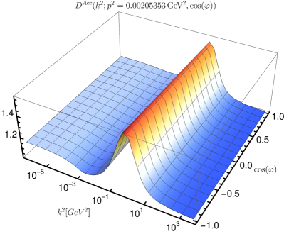
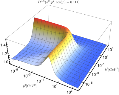
The results from a combined calculation of propagators and the ghost-gluon vertex are shown in Fig. 25. A comparison to lattice results is presented in Fig. 24. The general features of available lattice results are reproduced, viz., there is a bump in the midmomentum regime and the dressing goes down to one at zero momentum. A noteworthy anomaly concerns the scale of the bump for the gauge group [237]. All continuum results have the bump at a lower scale than the lattice results [176, 334, 305, 336, 188, 51, 24].
Three-gluon vertex
The three-gluon vertex is a crucial ingredient for the solution of the gluon propagator DSE as discussed in Sec. 4.2.2. An important property of initial models was a UV behavior that leads to a consistent UV behavior of the gluon propagator DSE [415]. Lattice calculations in lower dimensions indicated later [235, 237] that the tree-level dressing of the three-gluon vertex could become negative in the IR. In first exploratory continuum studies it was found that the ghost triangle indeed becomes negative [495]. The first full calculation was then done for two dimensions and the zero crossing was confirmed [175]. By now this feature was found in many approaches, e.g., [305, 91, 177, 496, 55, 497, 498, 66, 188, 94, 52, 24]. Also lattice methods find evidence of it [499, 263, 262, 264], although the low position of the crossing makes a definite confirmation difficult. Continuum methods show that the vertex diverges logarithmically in four dimensions [305, 91, 177, 55, 188, 52, 24]. The possibility of additional kinematic IR singularities, viz., only one momentum goes to zero, was ruled out for the decoupling solutions [355, 350]. For the scaling solution they can be present, although they are weaker than the overall IR ones [355, 171, 500, 350]. It should also be noted that the creation of a gluon mass gap is related to a potential IR irregularity of the vertex [75, 501, 184]. Perturbatively the full momentum dependence of the vertex is known up to two-loop order [487]. More perturbative studies can be found, for example, in Refs. [327, 502, 488, 489, 490, 491, 492, 493, 487]. String inspired methods for the decomposition of the vertex [503] are also known [504, 505, 506, 507].
A model that implements this zero crossing is given by [176]
| (206) |
where the UV part is (with , and )
| (207) |
and the IR part
| (208) |
with the damping factors
| (209) |
The exponents and can be determined such as to reproduce the correct anomalous running and make the vertex finite at zero momentum. For decoupling one obtains and and for scaling and , see also below Eq. (177). The parameter is typically chosen as . The scale can then be used to move the zero crossing. To obtain the correct anomalous dimension of the gluon propagator in a one-loop truncation, the final expression used for the three-gluon vertex is (see Sec. 4.2.2 for details)
| (210) |
It turned out that this model can be used to obtain a gluon propagator in good agreement with lattice results. However, it was clear that with the choice of parameters required for that agreement, the model can only be considered an effective model, because the zero crossing was at momenta so high that there was a clear disagreement with lattice results. Nevertheless, results from this calculation, which are shown in Figs. 27 and 28, proved as useful input for subsequent studies of vertices.
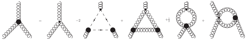
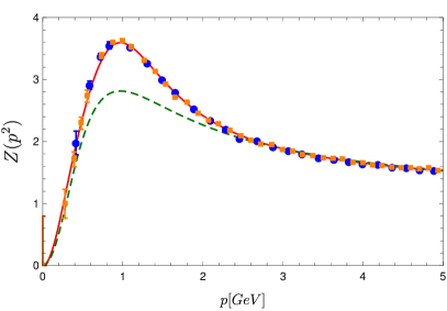
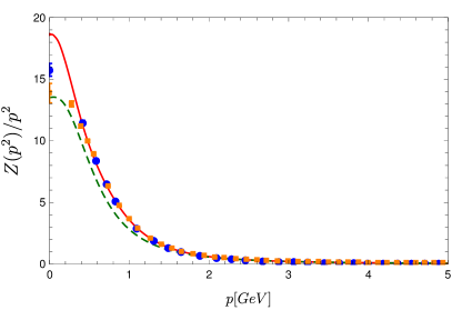
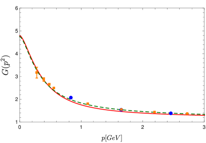
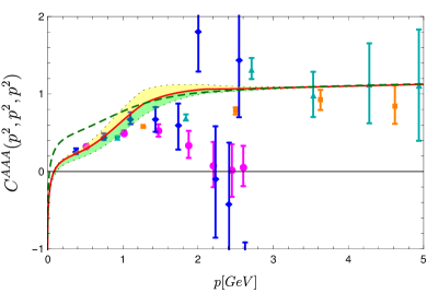
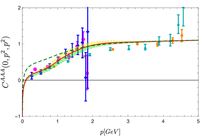
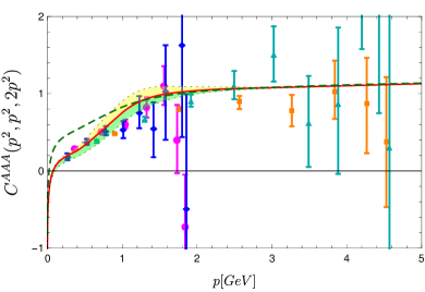
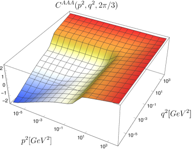
First dynamical calculations of the three-gluon vertex were done in Refs. [177, 55]. Using a modern form of the gauge technique, the longitudinal parts of the three-gluon vertex were also calculated [52]. All these calculations confirmed the existence of the zero crossing. A comparison with lattice results for different kinematic configurations is shown in Fig. 29 [177]. The employed truncation is shown in Fig. 26. An important step when solving the equation is the manual symmetrization of the results. Since the Bose symmetry of the vertex is broken by the truncation, one has to restore it by hand by averaging over all three distinct permutations of the external legs. When this procedure is used, one can discard one swordfish diagram and multiply another one with as indicated in Fig. 26.
The results are shown in form of a band that was obtained by varying the parameters of the employed four-gluon vertex model given by
| (211) |
where and determines the additional IR interaction strength and the momentum scale of its onset. The exponents and are determined from the leading anomalous dimension of the four-gluon vertex, , and from the requirement that the vertex approaches a constant value in the IR. This yields and for decoupling and and for scaling. The qualitative agreement of the tree-level dressing with lattice results is quite good and it was shown in Ref. [55] that the other three dressing functions are smaller than the tree-level one. The vertex results from Fig. 29 were also fed back into the gluon propagator equation. To fix the UV behavior, the gluon loop was amended by Eq. (207) as RG improvement term. Assuming that the vertex results are close enough to the true form of the vertex, one can in this way estimate the importance of the missing two-loop diagrams in the gluon propagator DSE. The gap of the results to the lattice results can be interpreted as an estimate of the missing contributions of the two-loop diagrams [177]. In Sec. 4.2.3, the importance of two-loop diagrams was confirmed by a direct calculation.
Four-gluon vertex
The first truncations that were realized for the ghost-gluon and the three-gluon vertex DSEs involved models for the four-gluon vertex and set the other four-point functions to zero [333, 175, 176, 334, 177, 55, 66, 188]. A motivation for discarding the latter is that the corresponding diagrams are of order and thus suppressed in the UV. The diagrams with a four-gluon vertex, on the other hand, contribute to the leading perturbative order. It was also found that this vertex plays a role for the convergence of the three-gluon vertex DSE [177, 55, 188]. Thus, a more detailed analysis of the four-gluon vertex is of interest. Up to now this vertex was investigated with its DSE [508, 509, 510, 71, 511, 183, 512, 188, 513, 24], the FRG [184, 67, 189] and perturbatively up to one-loop for various kinematic configurations [502, 68, 514, 515], in particular the symmetric point [68, 514, 515]. String inspired methods for the decomposition of the vertex [503] are also known [516, 506].
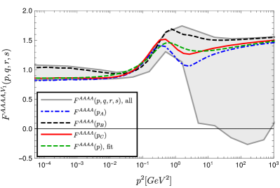
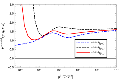
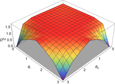
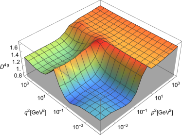
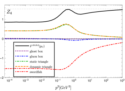
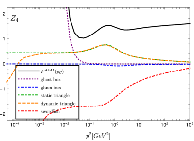
The four-gluon vertex is the most complicated four-point function, because it not only has four color indices but also four Lorentz indices as detailed in Sec. 2.2.7. Its DSE has 60 diagrams. 39 of them are two-loop and 20 are one-loop diagrams. For the presently employed truncation, all of the former are dropped as are all one-loop diagrams containing the two-ghost-two-gluon vertex (3 diagrams) or five-point functions (2 diagrams). This leaves 15 one-loop diagrams and the tree-level diagram. The impact of the discarded diagrams with two-ghost-two-gluon vertices is discussed in Sec. 4.2.5. However, the Bose symmetry of the four-gluon vertex allows reducing the number of diagrams to be calculated even further. If the complete kinematic dependence of a diagram is known, one can extract also the information about the diagrams obtained by permutations of legs. Thus, instead of calculating similar diagrams several times, only a single calculation is necessary. In total, five diagrams need to be calculated as can be seen in Fig. 5, where also the other one-loop diagrams are shown.
The employed truncation violates Bose symmetry. This can be repaired by averaging over all four distinct four-gluon vertex DSEs. Finally, there are twelve diagrams of each type which correspond to all possible permutations and the DSE is schematically calculated as
| (212) | |||
| (213) | |||
| (214) | |||
| (215) |
Here, is the transverse projection of the one-loop diagrams contracted with the tree-level tensor . The normalization is chosen such that the tree-level corresponds to one:
| (216) |
As another approximation, only the tree-level tensor out of the 41 transverse dressing functions is considered.
For solving the four-gluon vertex DSE in this approximation, fixed input given by the propagators from Refs. [176, 179], a bare ghost-gluon vertex and the three-gluon vertex from [177, 71] is used. Both decoupling and scaling type solutions are considered and the results are shown in Fig. 30 for three different kinematic configurations. The shaded area indicates the angle dependence which seems to be quite large. Fig. 31, however, shows that the angle dependence is in general very mild and only at the boundaries a strong dependence can be observed. As can be seen in Fig. 30, the dressing is very close to the tree-level. Thus, it is interesting to note that the contributions of the individual diagrams are not small by themselves but they largely cancel out as can be inferred from the results of the individual diagrams shown in Fig. 32.
Since the four-gluon vertex has many dressings, it is interesting to investigate if some of them are sizable. For a first impression, one can evaluate alternative projections of the four-gluon vertex DSE using the obtained results as input. The result for three projections is shown in Fig. 33. As can be seen, they are not larger than the corrections to the tree-level projection. Thus, within the tested set of tensors, the tree-level tensor is dominant due to its constant contribution from the bare vertex.
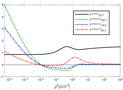
Two-ghost-two-gluon vertex
Landau gauge Yang-Mills theory has two non-primitively divergent four-point functions, the two-ghost-two-gluon and the four-ghost vertices. For the scaling type solution it is known that diagrams with the two-ghost-two-gluon vertex can belong to the class of IR leading diagrams [348]. Neglecting them does not change the scaling laws themselves, but in a quantitative study, the contributions of these diagrams might be important. If this is true for scaling, one might expect that for decoupling they might play a similar role. Thus, a detailed study of their influence on lower correlations functions is warranted. Perturbatively this vertex was studied in Ref. [515] and with its DSE in Ref. [188].
The two-ghost-two-gluon vertex, being non-primitively divergent, does not appear in the Lagrangian density. Thus, its lowest perturbative order is one order higher than that of the four-gluon vertex. Its impact in the midmomentum regime is hardly studied due to the technical complexity of corresponding calculations. However, its structure reveals a few simplifications that alleviate its study. This also includes the fact that its DSEs can be truncated such that almost all contributions are retained as discussed below.
As the ghost-gluon vertex, the two-ghost-two-gluon vertices has formally three different DSEs. The two with the ghost and anti-ghost legs attached to the bare vertex can be transformed into each other by exchanging ghost and anti-ghost. They yield identical equations. The third equation, with the gluon leg attached to the bare vertices, is the more complex equation due to the appearance of two-loop diagrams. Thus, the equation with the ghost attached to the bare vertices is used here, see Fig. 6. The employed truncation discards only one diagram, namely the one containing a five-point function.
The study of the two-ghost-two-gluon vertex is complicated by the absence of a tree-level tensor which is a good first approximation of the full tensor bases in case of the three- and the four-gluon vertices [55, 71, 512]. A possible guide could be the fact that the anti-symmetric structure constants contracted with the vertex in the corresponding diagrams of the ghost-gluon and three-gluon vertex DSEs annihilate the color part symmetric with respect to the two corresponding legs. However, in the generation of the relevant dressing functions the complete color space may play a role. Thus, the full basis as given in Eq. (73) is used.
The kinematic dependence of the two-ghost-two-gluon vertex is approximated by a single momentum scale. Given the size of angle dependences observed in three-point functions, see, for example, Fig. 25, the error induced in the two-ghost-two-gluon vertex, which is smaller in magnitude than the three-point functions, is expected to be small. The advantage of this approximation is that calculations are much faster compared to calculations of the full kinematic dependence with six variables [71]. The chosen kinematic configuration is the average of the squared momenta:777The same variable name is used for all -point functions, since it is clear from the context the average of which momentum squares is meant.
| (217) |
To calculate the 40 individual dressing functions , the DSE of the two-ghost-two-gluon vertex is contracted with the basis tensors yielding 40 scalar equations. Due to the non-orthogonal basis, the dressing functions are extracted by multiplication with the corresponding rotation matrix , where is given by
| (218) |
The chosen basis leads to dimensionful dressing functions. For plotting, it is advantageous to work with the dimensionless dressing functions instead by multiplying with appropriate power laws:
| (219) |
The are the dimensions of the dressings given by the negative dimensions of the basis tensors. Thus, the quantities reflect the actual momentum behavior that enters in other equations. Power laws with the dimensions of the dressings are also used for the UV extrapolations. The suppression from these power laws is crucial to avoid spurious UV contributions.
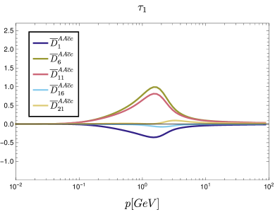
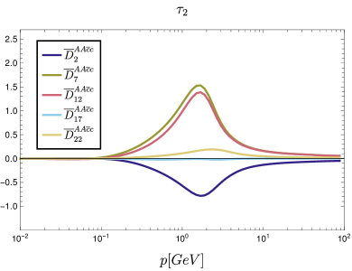
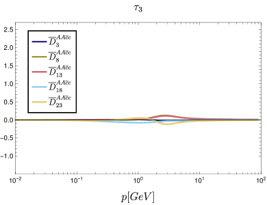
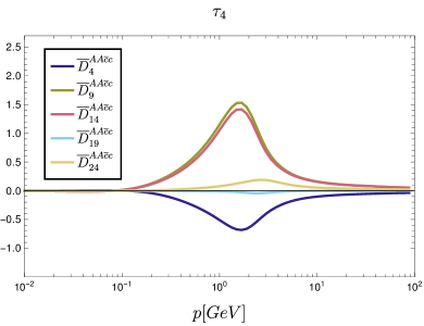
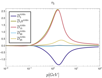
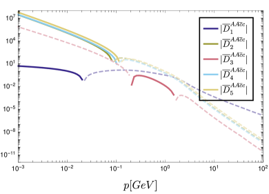
The two-ghost-two-gluon vertex is calculated together with the ghost-gluon, three-gluon and four-gluon vertices for which also one-configuration approximations are used. In their DSEs, the diagrams with the two-ghost-two-gluon vertex were included. The propagators are taken as fixed input and correspond to the results shown in Fig. 22. In this context it should be noted that the dynamic inclusion of the ghost-gluon vertex for the results of Fig. 22 is important, as otherwise the three-gluon vertex did not converge. This could be an artifact of the employed truncation and the sensibility of the three-gluon vertex DSE on the employed input in general. The results for the two-ghost-two-gluon vertex are shown in Fig. 34 in form of the dimensionless dressing functions . The behavior of the dressing functions in the UV shows that the leading behavior is, as expected, in agreement with the power laws from the dimensional analysis. In the IR, the dressing functions are power law suppressed compared to the UV. This is expected from a power counting analysis of the corresponding diagrams: Every gluon dressing function, behaving like in the IR, suppresses the integral. The power law behavior is exposed in the lower right image of Fig. 34 for a few dressing functions. The other five images show the 25 dressing functions corresponding to the reduced set of color tensors, see Sec. 2.2.7, grouped by their Lorentz parts. The scales on the ordinate have been chosen the same for easier comparison. Clearly, the largest dressing functions are those belonging to followed by those belonging to and . The group belonging to is basically negligible. Also the dressing function corresponding to the color tensors and are very small. These two are anti-symmetric under exchange of the two gluon legs, see Tab. 2.
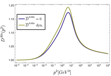
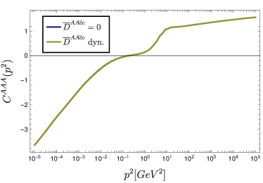
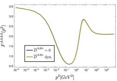
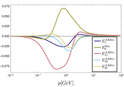
The dressings of the remaining three color tensors can be considered separately, because they decouple from the reduced set of color tensors. Projecting with these three tensors, only the diagrams with a two-ghost-two-gluon vertex remain. In this vertex, only these three color tensors remain so that this part of the vertex does not couple with the rest. It should be noted that this part of the vertex only contributes to the color symmetric part of the three-point functions, which, however, should be zero as discussed in Sec. 2.2.5. In the present case, the equation reduces in this color subspace to a homogeneous linear equation. For such an equation the trivial solution of all dressings equal to zero always exists. The attempt to find an alternative solution by starting from a simple ansatz always led to the trivial solution. A nontrivial solution cannot be excluded at this point, but it would be irrelevant due to the complete decoupling from the rest of the system of equations.
To assess the influence of the two-ghost-two-gluon vertex on other correlation functions, the same system as above can be solved without this vertex. The results for the ghost-gluon and the three-gluon vertices are shown in Fig. 35. Most remarkably, the three-gluon vertex does not change. This can be traced back to the color structure. In the three-gluon vertex DSE the gluon legs of the two-ghost-two-gluon vertex are contracted with an antisymmetric structure constant. Consequently, all contributions which are symmetric in the color indices of the two gluon legs vanish and only contributions from the color tensors and remain. However, Fig. 34 shows that these are the dressing functions which are very small. They cannot have any substantial influence on the three-gluon vertex. There could be indirect effects via the dependence of the other vertices on the two-ghost-two-gluon vertex, but as it turns out that they are not influenced largely either, this effect is tiny. In the four-gluon vertex the effect is also very small. Only the ghost-gluon vertex shows some difference, which, however, is at most.
Four-ghost vertex
The second non-primitively divergent four-point function is the four-ghost vertex. It was studied perturbatively in Ref. [515] and with its DSE in Ref. [188]. This vertex does not appear in the three-gluon vertex DSE. For the ghost-gluon vertex, it appears only in the -DSE. However, having the two-ghost-two-gluon vertex available, one can use the -DSE for the ghost-gluon vertex which is complete then and thus the preferred choice. At the four-point level, the four-ghost vertex does neither appear in the four-gluon vertex nor the -DSE for the two-ghost-two-gluon vertex. Hence, the four-ghost vertex does not couple back within this truncation.
The four-ghost vertex can thus be calculated a posteriori. Its setup is similar to the two-ghost-two-gluon vertex calculation. Its DSE is depicted in Fig. 7. Only one diagram is dropped in the truncation, namely the one with a five-point function. The full tensor basis, in this case consisting of eight color tensors, is employed, but the momentum dependence is approximated by a single momentum configuration. The result for the reduced color basis is shown in Fig. 35. The other three color tensors lead also in this case to a homogeneous linear equation for which only the vanishing solution is found.
4.3 Correlation functions of three-dimensional Yang-Mills theory
The study of Yang-Mills theory in three dimensions is interesting for several quite different reasons.888All results in this section were obtained for the gauge group , since all lattice results in three dimensions shown here are for this gauge group. However, within the employed truncations, the solutions are invariant under rescaling . First of all, the high temperature limit of four-dimensional Yang-Mills theory is a three-dimensional Yang-Mills theory with an adjoint Higgs field which is the leftover of the fourth component of the gluon field. This was studied, for example, in Ref. [485]. On the other hand, there are technical reasons as well for such studies. In lattice studies, three and also two dimensions were studied to reach lower momenta. For example, propagators were calculated in [234, 484, 237, 209, 211, 210, 235, 250, 236, 238, 229, 239, 240, 517, 232, 258, 259, 518, 233, 241, 337] and there are a few studies of vertices as well [235, 237, 337]. Studies of the Gribov problem are also simpler in lower dimensions [209, 211, 210, 240, 232, 258, 518, 241]. While the problem of reaching the deep IR does no exist for continuum studies, three dimensions are of interest as well, since they have a simpler UV behavior than four dimensions. This alleviates the treatment of spurious divergences as will be explained below. Further previous studies of the correlation functions of three-dimensional Yang-Mills theory were done with functional methods in [485, 348, 519, 171, 520, 91, 521, 512, 189], with the (refined) GZ framework in [522] and with a massive extension of Yang-Mills theory in [300, 315, 301, 305].
In this section I will present results for Yang-Mills theory in three dimensions obtained from the equations of motion of the 1PI and the 3PI effective actions. The employed truncation does not contain any model parameters and is fully self-contained. This allows studying modifications of this truncation to test its stability. Furthermore, the hierarchy of diagrams in the gluon propagator DSE is identified.
In the following, the differences between three- and four-dimensional Yang-Mills theory will be explained. Results for the primitively divergent correlation functions will be presented in Sec. 4.3.2. In Sec. 4.3.3 the stability of the employed truncation will be discussed and Sec. 4.3.4 contains a discussion of the results.
4.3.1 Specifics of three-dimensional Yang-Mills theory
In four dimensions, Yang-Mills theory is only logarithmically divergent due to gauge symmetry. Lowering the dimension by one, the theory becomes finite. One-loop diagrams behave then like , which can directly be inferred from the fact that the coupling has a mass dimension of . In addition, the UV finiteness leads to a trivial behavior under the renormalization group and, consequently, the absence of anomalous dimensions. This difference in the UV behavior makes three dimensions somewhat easier to treat numerically.
As discussed in detail in Sec. 4.2.1, the standard regularizations employed by functional methods break gauge covariance which entails the appearance of spurious divergences. In three dimensions, these spurious divergences are of degree one. As a remnant of resummation in four dimensions, also logarithmic divergences appear. This can be seen by considering that the one-loop UV behavior of the propagator dressings is of the form [523]:
| (220) |
In contrast to four dimensions, where the dressing functions behave logarithmically, the dressing functions in three dimensions become constant at asymptotically high momenta. Plugging the one-loop result into a one-loop expression, the second part lowers the degree of divergence by one leading to a logarithmic divergence proportional to . For dimensional reasons, it is obvious that no divergences can arise from higher orders in since the mass dimension of must be canceled by a corresponding momentum. This reflects the absence of resummation in three dimensions.
The general form for the divergent term in three dimensions is then
| (221) |
The coefficients and can be calculated perturbatively [512]. A term proportional to [523] would require a quadratic cutoff dependence, which, however, was not found in the actual calculations. However, once full vertices and propagators are employed numerically, this influences their values. In the present truncation, differences of up to were observed. Thus, it is best to fit the coefficients to the cutoff . In this way, also two-loop diagrams can be handled without having to calculate them analytically in the perturbative regime. Furthermore, the contribution of the tadpole diagram is automatically absorbed in , as it can produce only powers of the cutoff or a logarithm thereof. The perfect agreement of the fit with the analytic result can be illustrated by plotting , where corresponds to the unrenormalized right-hand side of the DSE, see Fig. 36. The reason for the perfect agreement is that the fit function contains all possible dependencies on the cutoff , namely and . This is different in four dimensions where fitting is thus not practicable. The subtraction coefficient must indeed be known very precisely. As an example, consider the solution when it is artificially modified as as shown in Fig. 36. Any larger change has a correspondingly larger influence.
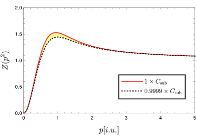
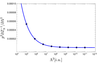
The subtraction of spurious divergences contains a possible ambiguity, namely, a constant term can always be added to without changing the asymptotic UV behavior or the cutoff independence of the results. Thus, technically the subtraction term can be used to generate a family of solutions. In this case, instead of fitting , it is set such as to obtain a given value for the gluon propagator at zero momentum in a similar way as discussed in Sec. 4.2.1. In Fig. 37, this possibility is shown for a simple test system that consists of the propagators and uses bare vertices [512]. Clearly, different solutions arise akin to the family of decoupling solutions. However, since the back reaction on the vertices is not contained in the system, the observed effects are most likely larger than they would be in a more elaborate truncation. It should also be noted that the ghost dressing function is not set to any value in the IR and, hence, there is only one effective parameter for choosing different solutions. In fact, it was found that doing so leads to the wrong UV behavior of the form with . In four dimensions, the procedure of fixing the ghost dressing function via a boundary condition [53] does not face this problem because of the anomalous running of the dressings.
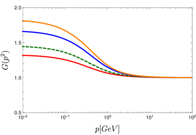
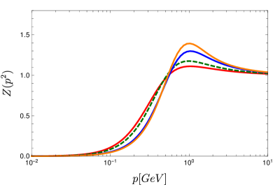
As mentioned above, the coupling is dimensionful in three dimensions. Thus, one could express all dimensionful quantities as multiples of powers of . A physical value is determined using lattice results where the scale is set via a string tension of . To transfer this scale to the continuum results, the peak of the gluon dressing function is matched to that of lattice results. However, since the heights of the dressing functions are not the same, one has some freedom to match the forms of the peaks. From this an interval of to around the lattice maximum is used to set the continuum maximum. In the plots where a band is shown, it represents this freedom in setting the scale. In plots with single lines, the maxima are matched using a value of .
4.3.2 Results for the primitively divergent correlation functions
Before the details of testing the truncation dependence are discussed, I present the results for all primitively divergent correlation functions and compare them to lattice results in the minimal Landau gauge. The results shown below were calculated with the largest truncation up to date: The propagator equations were fully included and the vertex equations were truncated to the perturbative one-loop level. In other words: All correlations functions are dynamical except for the non-primitively divergent ones which are set to zero. For the three- and four-gluon vertices only the dressings of the tree-level tensors were used.
The result for the ghost propagator is shown and compared to lattice results in Fig. 38. Below , the DSE result is systematically below the lattice result. Since the equation for the ghost propagator is complete, the source of this discrepancy must be caused by deviations in the other correlation functions. Such deviations are indeed found, as discussed below. The sensibility of the ghost dressing function on the gluon propagator was already visible in Fig. 37. However, also the existence of a family of solutions is reflected in the ghost propagator. Thus, the overall effect is most likely a mixture of both.
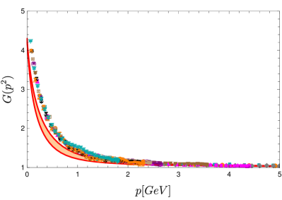
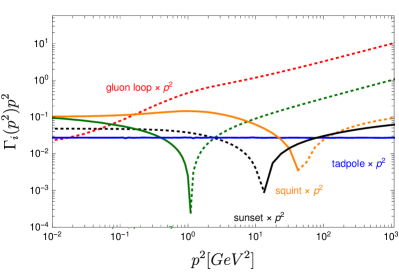
For the gluon propagator there is also a difference to lattice results. It is largest in the midmomentum regime. In particular, the peak in the dressing function is lower than in lattice results. As for the ghost propagator, the existence of the family of solutions has most likely an effect here. In particular, one can see in Fig. 37, that the height of the bump varies for different solutions. In addition, while the equation for the gluon propagator is complete in terms of diagrams, two vertices are not taken with their full tensor structure. Thus, those missing contributions may also have their share in the missing strength of the gluon dressing function.
Calculating each single diagram from the obtained solution, one can also assess the quantitative importance of single diagrams. Spurious divergences are subtracted in the same way as for the full equation, viz., by fitting the cutoff dependence. Note that for other methods it might not be possible to calculate individual diagrams. The contributions of all five diagrams are shown in Fig. 38. The hierarchy in the UV is as expected: The one-loop diagrams are dominant with the gluon loop being larger than the ghost loop as expected perturbatively. In the low momentum regime, the ghost loop becomes important. The sunset diagram is overall very small. The second most important contribution in the midmomentum regime comes from the squint diagram. As far as two-loop diagrams are concerned, it is interesting to see that the squint diagram clearly dominates over the sunset diagram. However, one has to bear in mind that in this calculation only restricted tensor bases for the gluonic vertices were taken into account and it cannot be excluded that the full bases would alter the relative importance of the diagrams.
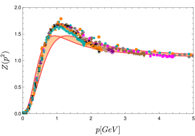
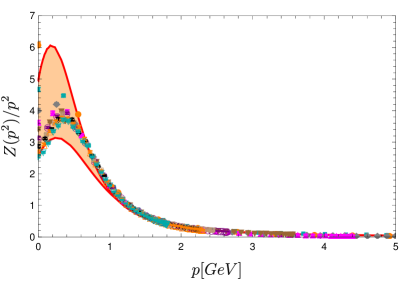
As discussed in Sec. 2.2.4, the ghost-gluon vertex has two DSEs. Here, the one with the bare vertex attached to the ghost leg is employed. The obtained dressing function features some angle dependence. In particular, the height of the bump around varies. The contributions of the two diagrams contained in the employed truncation are shown in Fig. 40. As can be seen, the non-Abelian diagram is the more important one. The comparison to lattice results [237] shown in Fig. 40 makes evident that the position of the bumps do not match. This is also known from results for the gauge group in four dimensions, see Sec. 4.2.5. A change in scale within the range discussed in Sec. 4.3.1 is insufficient to explain this. The source of this discrepancy is currently not known.
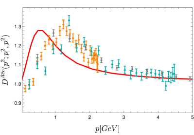
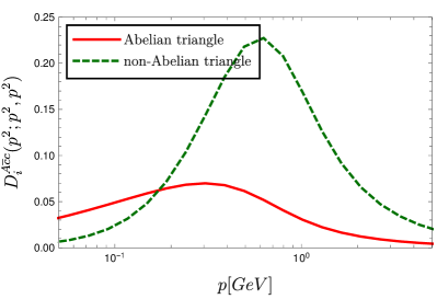
The three-gluon vertex has only a small angle dependence. The structure of the dressing function is very simple, being close to one, the asymptotic value, at high momenta and only moving away below . In the IR it diverges linearly. In general, the result is remarkably close to lattice results [237]. Seeing this structure, it is surprising to find that the individual diagrams are not small. They start to deviate from zero roughly below . The smallness of deviation from the tree-level is thus the consequence of cancellations between the contributions of the individual diagrams. Only the ghost triangle is not compensated and causes the divergence in the IR.
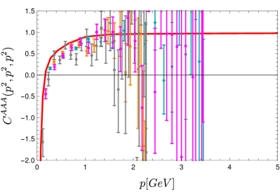
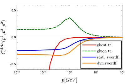
The last correlation function to be discussed is the four-gluon vertex. Similar to Sec. 4.2.5, three specific configurations are chosen for illustration purposes. The calculation itself was done for the full momentum dependence. As can be seen in Fig. 42, there is a similar pattern as for the three-gluon vertex although not as extreme. Still, the deviation from the tree-level is small. The dominant contribution at low momenta is again the ghost diagram. The gluonic diagrams, on the other hand, partially cancel each other. As can also be seen in Fig. 42, the four-gluon vertex has a stronger angle dependence, at least in the variables chosen here, than the three-gluon vertex. To get an idea about the possible influence of other dressing functions not taken into account, alternative projections were evaluated taken the previously obtained solution as input. The results for three further projections including the corresponding contributions from single diagrams is shown in Fig. 43. The only sizable contributions appear around , but compared to the tree-level dressing, which gets a constant contribution from the tree-level diagram, they are small.
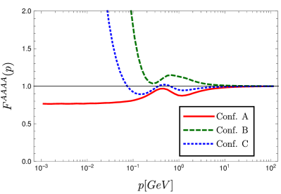
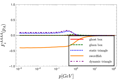
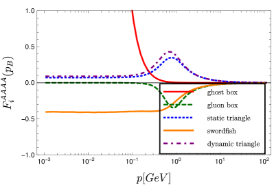
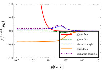
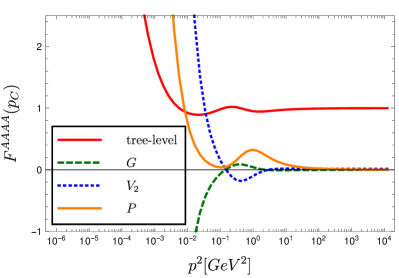
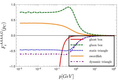
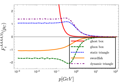
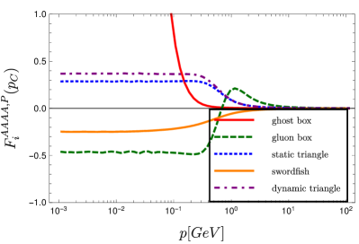
Finally, the couplings as extracted from the different vertices, see Eq. (171), are shown in Fig. 44. The couplings from the ghost-gluon, the three-gluon and the four-gluon vertices agree very well from the perturbative regime down to a few GeV.
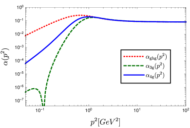
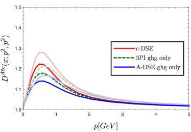
4.3.3 Testing the truncation
While the truncation used in the previous section is already quite large, it is not clear whether it is already sufficient to obtain quantitatively reliable results. However, since the truncation is large enough, it allows various modifications to test the influence of different parts. For small truncations such tests are often not possible, because all the ingredients are crucial and tampering with them too much changes the solution drastically. In this section, the truncation dependence is tested in two different ways. First, the influence of choosing different equations is tested. Second, the influence of the highest included correlation function, the four-gluon vertex, is assessed.
As explained in Sec. 2.2.4, the ghost-gluon vertex has two different DSEs, one with the gluon leg attached to the bare vertex, the -DSE, and one with the ghost leg attached to the bare vertex, the -DSE. The ghost-gluon vertex also fulfills an equation of motion derived from the 3PI effective action, see Fig. 2. Here, the results from all three equations are tested. The two DSEs are truncated to the two triangle diagrams. The difference between the three equations lies only in the number and position of dressed vertices. One should keep in mind, though, that the truncations drop a different number and different types of diagrams: For the -DSE, nine diagrams are dropped (seven two-loop diagrams and two one-loop diagrams containing a quartic ghost vertex or a two-ghost-two-gluon vertex) and for the -DSE only one diagram containing the two-ghost-two-gluon vertex is dropped. The 3PI effective action is expanded up to three loops. The resulting equation of motion contains the same diagrams as the DSEs, but all three vertices are dressed. So while formally the truncation specified above is the same in all three cases, it has different effects on the equations. The resulting difference can thus be interpreted as the systematic error of this truncation.
For this comparison fixed input from the full system discussed in Sec. 4.3.2 is used to avoid a backcoupling of the truncation effects. Fig. 44 shows the results for two different kinematic configurations from the three equations. The contributions of single diagrams are shown in Fig. 45. Taking as a measure of the truncation error the maximum of the ratios of dressings, we obtain . The difference for the configurations shown is even lower and typically below .
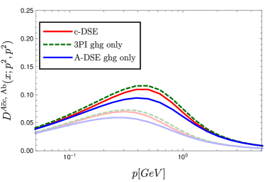
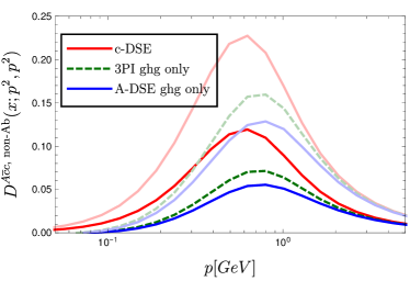
As a second test, the full system was calculated with the equations of motion from 1PI and 3PI effective actions. For the DSE system, the -DSE was used. The ghost dressing functions from the two systems differ only below , see Fig. 46. For the gluon propagators the situation is similar and the main difference in the gluon dressing functions occurs at , see Fig. 47. Fig. 48 shows the differences for the ghost-gluon and three-gluon vertices. For the former, it is similar to the ghost-gluon vertex-only calculation discussed above and depicted in Fig. 44. For the three-gluon vertex the main difference is a shift of the zero crossing for the 3PI system towards the IR. Overall the differences between the DSE and the 3PI setup are relatively small with the largest effects observed in the deep IR.
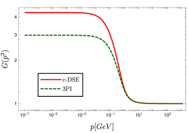
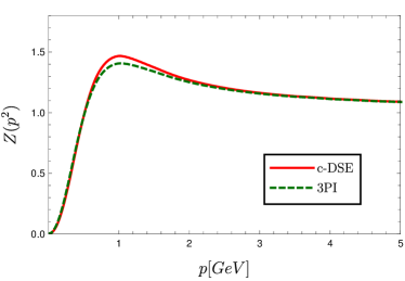
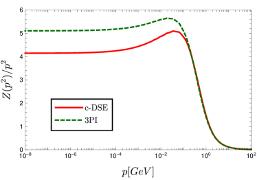
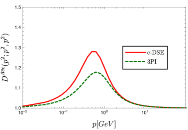
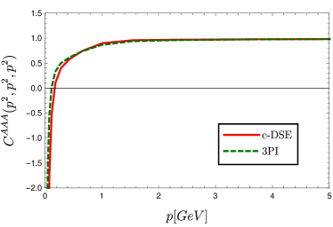
Finally, the effect of the four-gluon vertex is discussed. The corresponding results of this vertex, which show only a small deviation from the tree-level behavior, suggest that it has only a minor influence on lower correlation functions. It appears in the gluon propagator and the three-gluon vertex equations and we already saw that the corresponding diagram in the former, the sunset diagram, has only a minor quantitative influence. The ghost propagator and the ghost-gluon vertex are only influenced indirectly. To quantify the effects, the system is solved with a bare four-gluon vertex and compared to the results from Sec. 4.3.2. The comparison is shown in Fig. 49 and Fig. 50. Clearly, the effect is very small indeed. However, it should be noted that the four-gluon vertex plays a decisive role in the convergence of the three-gluon vertex DSE in four dimensions as mentioned in Sec. 4.2.5.
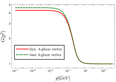
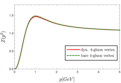
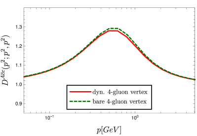
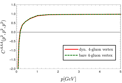
4.3.4 Discussion
Overall, the tests of the truncation performed here show that the changes are only of quantitative nature. On the one hand, it is promising that finally a truncation was found that exhibits this degree of stability. First of all, because simpler truncations are more sensitive to the input, and second, because the present truncation does not have the freedom to tune any model parameters. On the other hand, the question is now why there is still a discrepancy to results from lattice calculations. Several possible explanations exist.
First, one must ask how meaningful a quantitative comparison between lattice and continuum results is at all, because the ways how the gauge is fixed in the two methods are different and no direct one-to-one correspondence is known. The dependence on the gauge fixing algorithm is well established on the lattice for three [211, 240, 232, 215, 258] and also four dimensions [204, 206, 494, 211, 232, 213]. Results exist [215, 241] where the difference between two ghost dressing functions is at and even more below. As demonstrated in Sec. 4.3.1, also with functional equations different solutions can be obtained. However, at the moment it is not clear how close the present results should be to the lattice results using the minimal Landau gauge, because the gauge employed here is most likely a different gauge.
Of course, another source for the differences are contributions that are still missing in the continuum results. There are two types of such contributions: Incomplete equations and incomplete tensor bases. In the present truncation, neither applies to the propagators and the latter also does not apply to the ghost-gluon vertex.
For the ghost-gluon vertex different equations were tested in Sec. 4.3.3. The found differences of the order of can clearly be attributed to truncation artifacts. Thus, it will be necessary to include more diagrams and check how the results change. In case of the -DSE, this requires only the two-ghost-two-gluon vertex, which was discussed for four dimensions in Sec. 4.2.5, to make the equation complete, whereas the -DSE contains two-loop diagrams as well.
In addition to missing diagrams, the calculation of the three-gluon vertex also lacks a full tensor basis. In four dimensions, the three-gluon vertex DSE was solved with fixed input with a full tensor basis [55]. It was found that the dressing of the tree-level dressing is the dominant contribution and the other three transverse dressings are quite small. This should hold also in three dimensions and hence one would expect the effect of completing the basis to be correspondingly small. However, one should not forget about the non-linearity of the equations which could make the suppressed dressings at least somewhat important. On the other hand, the three-gluon vertex shows the best agreement with lattice results. From this one would expect that the truncation works quite well for this particular quantity.
For the four-gluon vertex, the cancellations between diagrams do not work as well as for the three-gluon vertex. In addition, there are many more dressing functions so that the sum of even small contributions could, if no cancellations appear, be sizable. Thus, for the four-gluon vertex the choice of a proper basis could well be quite important. An enlarged tensor basis could also change the importance of the sunset diagram if additional tensors are taken into account.
In summary, there remain a few extensions of the present truncation the effects of which still have to be tested. In the meantime, it is reassuring that with the FRG results with similar deviations from lattice results were found [525, 189]. Taking into account also information from four dimensions, extensions of the three and four-gluon vertex bases currently seems to be a promising approach, especially since these vertices directly enter in the gluon propagator DSE.
4.4 Correlation functions of two-dimensional Yang-Mills theory
Yang-Mills theory in two dimensions is another testing ground for lattice and functional methods. One of the reasons for a more detailed investigation with lattice methods was the hints found in three and four dimensions that the three-gluon vertex could become negative at low momenta [235, 237]. A calculation in two dimensions can probe even deeper into the IR. Besides the confirmation of the zero crossing of the three-gluon vertex, it was also found that the correlation functions in two dimensions behave qualitatively different to three and four dimensions in the IR regime [230]. Within the available statistics, the scaling solution seemed to be realized for propagator and vertices [352, 230, 348]. Later studies, however, raised some questions, since the scaling laws seem not to respect the sum rule [256, 210, 526, 239, 518].
The absence of a decoupling solution sparked some additional interest in the study of two-dimensional Yang-Mills theory. A study with the (refined) GZ framework found that the condensates responsible for making the gluon propagator finite in three and four dimensions do not exist in two dimensions due to IR divergences [527]. Also in other approaches, IR divergences were found to play a decisive role [300, 301, 315, 528, 175, 529].
In DSE calculations the relevant divergences appear in the ghost propagator equation. They need to be counteracted by a gluon propagator that vanishes at zero momentum [528]. This holds as long as the ghost-gluon vertex does not vanish itself, which, however, is not found in explicit calculations [175]. Note, though, that these calculations of the vertex are done for the scaling case. For the vertex to vanish at zero momentum in the decoupling case, the contribution of the tree-level would need to be canceled by the loop contributions. Thus, a decoupling solution is unlikely to be realized in two dimensions. Quantitatively, for the decoupling case the IR divergences lead to an explicit dependence on the IR cutoff as shown in Fig. 51.
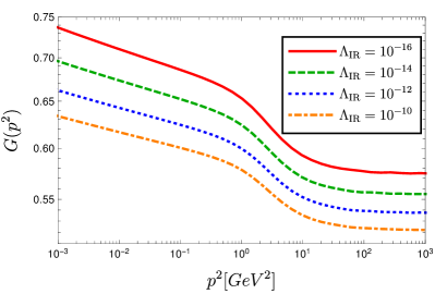
Another effect in two dimensions is the mixing of different momentum regimes. In four dimensions, a clear separation is possible. For example, the UV behavior can be determined self-consistently without referring to low scales. In three dimensions, the influence of different momentum regimes on each other is already noticeable [485, 183], see also Sec. 4.3. However, a perturbative calculation can still be performed for high momenta. In two dimensions, on the other hand, perturbation theory does not work anymore again due to arising IR divergences. They are cured by the nonperturbative behavior of the gluon propagator that vanishes at zero momentum. Thus, the asymptotic high momentum behavior in two dimensions can only be determined qualitatively from dimensional arguments as
| (222) |
The coefficients and can be determined numerically in a nonperturbative calculation.
The strong entanglement of different momentum regimes makes it difficult to recover the correct UV behavior in a truncated system, since any defects in other regimes have an impact on the UV regime. This problem appears also in three dimensions but is less severe there, see Sec. 4.3. However, as long as models are used for the vertices, once can use them to tune the UV behavior of the dressing functions to approach in the UV.
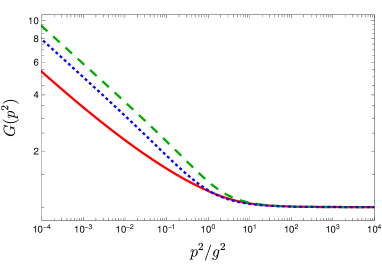
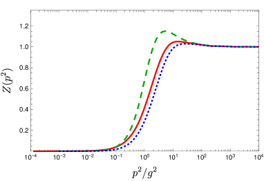
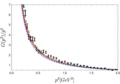
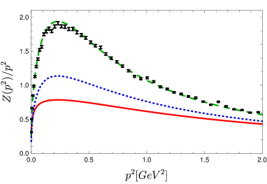
Truncating the system of propagators to the one-loop diagrams without tadpole diagram [175], only the ghost-gluon and three-gluon vertices are required. In the following, three choices for the vertices will be tested. Two use a model for the ghost-gluon vertex and one includes it dynamically. In the former case, it is once taken as bare and once the following model is employed:
| (223) |
For the three-gluon vertex, two models will be tested. The first one, which is constructed to mimic the known behavior of the vertex, is
| (224) |
The correct UV behavior is ensured by the second term, whereas the first term implements the IR divergence [175]. Choosing negative leads to a zero crossing. The position of the zero crossing resulting from the employed parameters is higher than one would expect from lattice results. In this way, the gluon loop can make up some missing strength coming from the neglected two-loop diagrams. An alternative model, inspired by a model in three-dimensions [485] that was created before the qualitative IR behavior of the vertex was known, is
| (225) |
The three combinations of vertices tested in the following are:
-
•
A bare ghost-gluon vertex and Eq. (225) for the three-gluon vertex.
- •
-
•
A dynamically coupled ghost-gluon vertex and Eq. (224) for the three-gluon vertex.
The parameter values for the models are listed in Tab. 4.
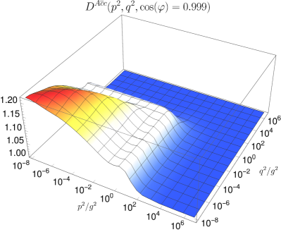
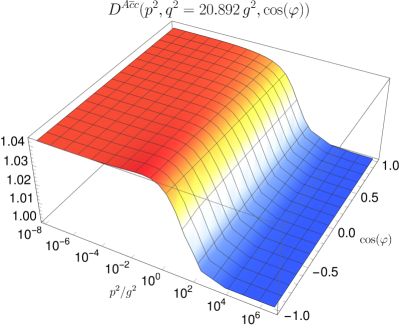
Two-dimensional Yang-Mills theory is in principle superrenormalizable. However, also here spurious divergences arise in the gluon propagator DSE, see Sec. 4.2.1. They are logarithmic and appear in the following form:
| (226) |
Here, is logarithmically divergent and is finite. The logarithmic divergence can be handled by a subtraction of the self-energy at multiplied by :
| (227) |
Alternatively, other methods discussed in Sec. 4.2.1 could be used.
| Ghost-gluon vertex | Bare | Model 223 | Dynamic | |||
|---|---|---|---|---|---|---|
| Three-gluon vertex | Model 225 | Model 224 | Model 224 | |||
The results for the three setups are shown in Fig. 52. Clearly, the models have a large impact on the midmomentum regime. The ghost-gluon vertex result is shown in Fig. 53. Due the large deviations between the functional and the lattice results in the propagators of the combined calculation, the agreement of the ghost-gluon vertex result with lattice results is not very good either [175]. The employed level of truncation is rather basic, though, and it would be interesting to see how the results of all quantities would change in a more elaborate truncation as used in Sec. 4.3 for three dimensions.
For the three-gluon vertex, results are shown in Fig. 54. They were calculated from the solution of the propagators and the ghost-gluon vertex using a bare four-gluon vertex. The employed truncation is the same one used in Sec. 4.3, viz., all diagrams with two loops or non-primitively divergent vertices are discarded. This provides the correct IR behavior and includes also the leading corrections to the tree-level behavior in the UV. Fig. 54 also shows the effect of different diagrams. Clearly, the ghost triangle is leading in the IR. As in higher dimensions, a cancellation between the gluon triangle and the swordfish diagrams is observed: The gluon triangle introduces a bump in the dressing which is removed completely by the inclusion of the swordfish diagrams.
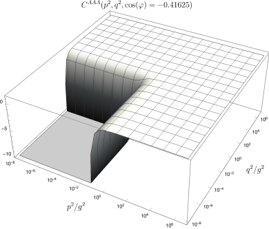
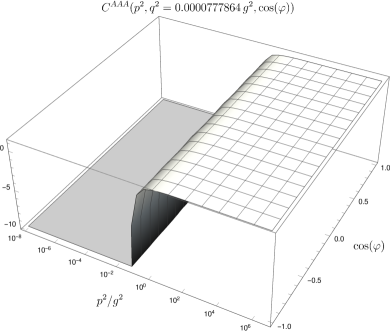
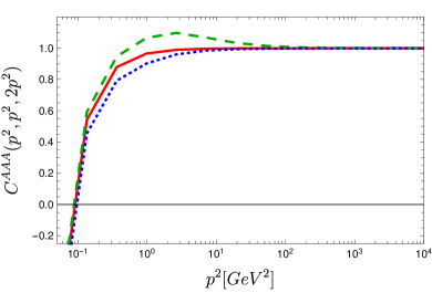
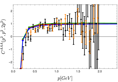
In summary, two-dimensional Yang-Mills theory, for which vertex DSEs were solved for the first time self-consistently, proved to be a useful testing ground for developing the necessary methods and get a first impression of the general problems like cancellations between diagrams in the gluonic vertices. The results also hinted at the fact that, in the absence of resummation, the three-gluon vertex can be recovered in good agreement with lattice results, while a good description of the propagators is more difficult.
5 Correlation functions in different gauges
The correlation functions of quarks and gluons are necessarily gauge dependent. As explained in Sec. 4.1, the Landau gauge has many advantages that make it very convenient to work with. However, beyond that, also other gauges are investigated. An obvious reason for using different gauges is to check the gauge dependence of gauge invariant quantities introduced by the truncation. Another reason to investigate different gauges is that they might provide alternative perspectives at specific physical problems. For example, the color-Coulomb potential, viz., the instantaneous part of the -component of the gluon propagator in Coulomb gauge, is related to the potential of a quark–anti-quark pair [530]. This is known as ’no confinement without Coulomb confinement’. Another example is the maximally Abelian gauge which allows the investigation of the Abelian dominance conjecture related to the dual superconductor picture of confinement.
In this section, results for various gauges beyond the Landau gauge are reviewed. The first example are linear covariant gauges in Sec. 5.1. The Landau gauge is actually just one specific gauge of this class. In Sec. 5.2, the maximally Abelian gauge is discussed and the Coulomb gauge in Sec. 5.3. Beyond these examples, infinitely many more gauges exist, for example, the axial gauge, the planar gauge, and the light-cone gauge, see, e.g., Ref. [531], or exotic ones like the Palumbo gauge [532, 533]. However, they are hardly used in functional equations and some gauges like the Laplacian gauge [534] are not accessible with functional methods at all.
Before the discussion of results from the different specific gauges, an interesting possibility should be mentioned here, namely the interpolation between different gauges. In the strict sense, also linear covariant gauges are such an interpolating gauge, but it is also possible to interpolate, for instance, between linear covariant and maximally Abelian gauges. However, with the different levels of sophistication in studies of different gauges, calculations using interpolating gauges are currently rather limited. Nevertheless, the prospect of connecting confinement scenarios that are more easily accessible in one or the other gauge makes them interesting for possible future calculations.
A prime example of an interpolating gauge is the so-called gauge which interpolates between the Landau and the Coulomb gauges via the gauge fixing condition
| (228) |
The case corresponds to the Landau gauge, while the limit corresponds to a Coulomb-like gauge. For an additional condition must be supplemented for a full gauge fixing condition. Note that also the Faddeev-Popov operator depends now on :
| (229) |
The gauge was studied on the lattice in Refs. [535, 536, 537].
Besides the Coulomb-Landau gauges example many other realizations of interpolating gauges exist, for example, formulations for interpolation between the Landau gauge and the maximally Abelian gauge [538, 151, 448]; linear covariant gauges, the Coulomb gauge and the maximally Abelian gauge [539, 540]; or linear covariant gauges, the maximally Abelian gauge and the Curci-Ferrari gauge [541].
5.1 Linear covariant gauges
The most natural choice of gauge beyond the Landau gauge are linear covariant gauges, also called gauges. They have the same gauge fixing condition as the Landau gauge, , but it is not enforced strictly. Rather, the gauge orbit is sampled around the Landau gauge with a Gaussian weight where the gauge fixing parameter determines the width:
| (230) |
The endpoint is the Landau gauge where the Gaussian distribution becomes a delta functional. For , the gauge field is not transverse. Consequently, the Faddeev-Popov operator is no longer Hermitian because of the term . Thus, its eigenvalues are not real as in the Landau gauge and a Gribov region cannot be defined in the same manner. However, there is a generalization of the Gribov-Zwanziger procedure [542] that can be applied also to linear covariant gauges [295].
For lattice calculations, the gauge fixing process of linear covariant gauges poses an additional challenge, since it cannot be formulated in the standard way as a minimization problem [543]. A suitable implementation was suggested in Ref. [544].
The relaxation of the gauge fixing condition entails that the gluon propagator in linear covariant gauges has a second dressing function. However, it is fixed by gauge symmetry via a corresponding STI. Thus, the gluon propagator has the form
| (231) |
Due to the longitudinal part of the propagator also the longitudinal parts of the vertices are relevant in functional equations. In the Landau gauge, on the other hand, it is straightforward to see that the transverse part constitutes a closed set [53].
In Sec. 5.1.2, results for the propagators in linear covariant gauges are presented. Details on how the longitudinal parts of the vertices are obtained are described in Sec. 5.1.1. There, also the dependence of correlation functions on the gauge fixing parameter is discussed using Nielsen identities.
5.1.1 Nielsen and Ward identities
In this section the Nielsen and Ward identities for linear covariant gauges are derived. The former, encoding the gauge parameter dependence, can be used to calculate correlation functions for different values of the gauge fixing parameter from a solution for a fixed value. The latter can be used to fix the longitudinal parts of correlation functions.
The fact that physical quantities must be independent of the gauge fixing parameter can be expressed via the Nielsen identity. One starts with the derivative of the effective action with respect to a gauge fixing parameter:
| (232) |
The notation from Sec. 3.1.1 was used where represents all classical QCD fields and the corresponding sources. For linear covariant gauges, we have . The Nielsen identity reads then
| (233) |
Equations for correlation functions can be obtained by applying further derivatives with respect to fields. For the ghost and gluon two-point functions, and , respectively, one obtains
| (234) | ||||
| (235) |
Following a different route, the explicit equations for the ghost and gluon propagators were also derived in [545].
Ward identities are derived from the invariance of the path integral under gauge transformations, see Refs. [546, 547, 139, 140] for details:
| (236) |
where the Ward operator ,
| (237) |
is the generator of infinitesimal gauge transformations. Eq. (236) is the generating equation for the Ward identities of all Yang-Mills correlation functions. By applying appropriate derivatives, the Ward identities for the ghost-gluon and three-gluon vertex follow. Keeping only the (dressed) tree-level terms, as indicated by , they read
| (238) |
for the ghost-gluon vertex and
| (240) |
for the three-gluon vertex. Note that the result for the three-gluon vertex does not assume any specific choice of basis tensors. The inhomogeneous terms of the ghost-gluon vertex are a direct consequence of the Faddeev-Popov term.
5.1.2 Propagators of linear covariant gauges from Dyson–Schwinger equations
Generally, linear covariant gauges have not been extensively investigated with the exception for their endpoint, the Landau gauge. In the following, I will only refer to the case , as the Landau gauge is discussed in detail in Sec. 4. Another special case of linear covariant gauges is the Feynman gauge, defined by . However, its special role is limited to perturbation theory because the gluon propagator reduces to the simple form at tree-level. This property does not extend to the non-perturbative regime, where the transverse part acquires a dressing. The case is called the Yennie gauge. Its special property is that the ghost one-loop self-energy becomes finite. The same happens for the gluon for the value .
In recent years, some progress has been made in nonperturbative investigations of linear covariant gauges: In lattice techniques the obstacle of how to fix the gauge was overcome [544, 548], and also continuum methods have shed some light on the nonperturbative behavior of its correlation functions [545, 182, 549, 296, 297, 550, 92, 551, 552]. The picture that has emerged during the last few years by combining several methods is the following: The gluon propagator is affected only very little by varying the gauge fixing parameter. In particular, it stays constant at zero momentum. This was seen in lattice calculations [548], Dyson–Schwinger calculations [182], the pinch technique-background field method (PT-BFM) [92] and the refined Gribov-Zwanziger framework [549, 296, 297, 550]. The ghost dressing function, on the other hand, vanishes logarithmically for , as seen with Nielsen identities [545] and DSEs [545, 182]. Also in the refined Gribov-Zwanziger framework this holds [296]. First lattice results do not reach far enough into the IR to say anything about the asymptotic behavior [553].
For , calculations are aggravated compared to the Landau gauge by the explicit appearance of the longitudinal parts of correlation functions. In the case of the gluon propagator, this can easily be handled, because the exact result is know from an STI, see Eq. (231). However, due to the necessary truncations, the calculation of the longitudinal part from its DSE or flow equation would show deviations from the exact result. For higher correlation functions, the STIs cannot be solved exactly. Alternatively, one can use Ward identities to derive closed expressions. The form of these equations is similar to DSEs and to render them useful they have to be truncated. As the simplest truncation, the UV leading terms can be kept, viz., only the tree-level terms are retained, see Sec. 5.1.1.
For an explicit calculation, also the transverse parts of the three-point functions need to be specified. As a minimal requirement, the models should obey the correct anomalous running in the perturbative regime. Since the ghost-gluon vertex is no longer finite for , it also runs logarithmically. This can be accommodated by the following model for the transverse part:
| (241) |
The exponents and are determined by demanding the correct UV behavior of the dressing. A natural choice for the second condition would be IR finiteness. However, this cannot be achieved, since the ghost dressing function vanishes logarithmically. So the exponents are determined assuming that the ghost dressing function is constant which should give a reasonable approximation. The exponents can be found in Tab. 6. The full ghost-gluon vertex is then given by
| (242) |
with
| (243) |
The three-gluon vertex consists of four transverse dressing functions. In the Landau gauge, the dressing of the tree-level term is dominant [55], so as a first approximation for the transverse part we will take into account the transversely projected tree-level tensor only. For the corresponding dressing function we make a similar ansatz as for the ghost-gluon vertex:
| (244) |
The exponents are determined in the same manor and can be found in Tab. 6. Whenever the three-gluon vertex is longitudinally contracted, Eq. (240) is used.
The anomalous dimensions of propagators and vertices are given in Tab. 5. The sum rules in linear covariant gauges are and .
Having specified these vertex models, the propagator DSEs can be investigated. First, the ghost propagator DSE is analyzed from which the IR behavior of the ghost propagator can directly be inferred. After plugging in Eq. (242), it reads
| (245) | ||||
| (246) |
where , and . From the third term in the parentheses, the IR behavior of the ghost dressing function can be determined [182]. For low external momentum it becomes
| (247) |
If were IR divergent or constant, this term would be IR divergent what would require the ghost dressing function on the left-hand side to vanish, in contradiction to the original assumption. Consequently, the ghost dressing function must vanish for low momenta. As no terms exist that would allow for a power law divergence on the right-hand side, corresponding to a power law suppression of the ghost dressing function, it must vanish logarithmically.
The gluon propagator DSE is truncated by retaining only the one-loop diagrams. Furthermore, the tadpole is dropped. The missing two-loop diagrams, however, would most likely contribute quantitatively. Thus, this study gives only a qualitative picture.
The level of truncation of this system of equations requires the usual additional tweak of using an RG improvement term discussed in Sec. 4.2.2 to obtain the correct one-loop resummed anomalous running. Here, in contrast to the Landau gauge, it is necessary also for diagrams with a ghost-gluon vertex, since the ghost-gluon vertex acquires an anomalous running for . Thus, also the ghost propagator DSE is affected. In addition, in the gluon loop several terms are required due to different combinations of dressing functions introduced by the longitudinal terms. The final equations read
| (248) | ||||
| (249) |
The detailed kernels are given in A.2. The renormalization group improvement is encoded in the function :
| (250) |
with . For different terms, different exponents and are required which are detailed in Tab. 6. They are determined such as to reproduce a self-consistent UV behavior of the equations while being constant in the IR assuming a constant ghost dressing function. The kernel contains additional factors of .
| Correlation function | Anomalous dimension |
|---|---|
| Ghost propagator | |
| Gluon propagator | |
| Ghost-gluon vertex | |
| Three-gluon vertex |
The spurious divergences in the gluon propagator DSE are subtracted analytically by subtracting the perturbatively calculated counterterms [179], see also Sec. 4.2.1. The corresponding coefficient of the subtraction term
| (251) |
is given by
| (252) |
Solving the coupled system of ghost and gluon propagator DSEs yields the results depicted in Fig. 55. The ghost dressing function vanishes in the IR as expected logarithmically, while the gluon propagator remains constant. The bump in the gluon dressing function becomes larger for increasing and moves to higher momenta. This shows that the employed truncation is not very suitable for higher values of the gauge fixing parameter, since the bump finally enters the regime which should be determined mainly by perturbation theory. For low momenta, on the other hand, the results should suffer only from the same quantitative effects as the equivalent solution for the Landau gauge to which it connects smoothly, viz., the missing two-loop terms lead to missing strength in the mid-momentum regime of the gluon dressing function.
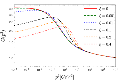
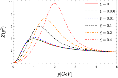
The results for the propagators in linear covariant gauges obtained with a simple truncation show that calculations with functional equations are feasible. To push such investigations further, also vertices need to be calculated. However, in that case the longitudinal parts could be problematic and it would be interesting to see how well the approximations of the Ward identities derived here work. Other improvements, like the inclusion of two-loop terms, which would discard the necessity of RG improvement terms, are expected to be straightforward.
5.2 Maximally Abelian gauge
The maximally Abelian gauge (MAG) is an example of a non-linear covariant gauge. It can be defined by a minimization procedure similar to the Landau gauge and is thus also amenable to lattice simulations in a standard way. The physical motivation for this gauge is the role played by the diagonal part of the gauge field in the dual superconductor picture of confinement. This gauge breaks the global color symmetry and treats the diagonal and off-diagonal parts separately. The plain MAG only gauge fixes the off-diagonal part and is thus an incomplete gauge fixing which has to be supplemented by an additional condition on the diagonal part. The standard choice for this is the Landau gauge.
In this section, investigations of the IR behavior of the MAG are presented. In general, investigations in this gauge are by far not as advanced as in the Landau gauge. The results presented here offer an explanation why this gauge constitutes a particular challenging gauge for functional equations.
5.2.1 The dual superconductor picture of confinement and Abelian infrared dominance
The dual superconductor picture of confinement explains confinement of chromoelectric charges by the QCD vacuum being a dual superconductor [554, 555]. In this scenario, chromoelectric charges are confined by chromomagnetic vortices which correspond to the flux tubes between quarks. Such vortices can form when chromomagnetic monopoles condense. The condensation of monopoles was observed later in lattice calculations [556, 557]. Motivated by the dual superconductor picture, an order parameter based on the chromomagnetic charge was developed [558, 559, 560, 561, 562, 563]. By choosing a certain class of gauges, the so-called Abelian gauges, monopoles can be identified [564, 565]. These gauges impose only a partial gauge fixing and leave the Abelian part of the gauge field unfixed. For a theory with gauge group , this is the subgroup . There are infinitely many possibilities to realize an Abelian gauge. One is the maximally Abelian gauge (MAG), in which the gauge field itself is made as Abelian as possible. Thereby, Abelian refers to the part of the gauge field living in the Cartan subalgebra, which consists only of diagonal matrices and is thus also referred to as diagonal part.999The Cartan subalgebra is defined by the generators that commute with all other generators. For , this is and for and , where are the Pauli matrices and the Gell-Mann matrices. For general , the Cartan subalgebra consists of the matrices (253) The gauge field is maximally Abelian if the norm of the parts of the gauge field not in the Abelian subalgebra is minimized.
Based on the assumption that chromomagnetic monopoles cause confinement, Ezawa and Iwazaki conjectured that the Abelian parts of the gauge fields should be dominant at large distances, since classic magnetic monopoles live in the Cartan subalgebra [566]. This conjecture is called Abelian IR dominance. Indeed, for many quantities it is observed that they are only slightly affected by removing the off-diagonal part, a procedure called Abelian projection. For example, the string tension between a static pair of quarks has almost the same value if calculated from the diagonal part of gauge fields alone or from the complete fields, see, for example Refs. [567, 568]. An extension of Abelian dominance is monopole dominance. In that case, only the monopoles are retained and still many observables remain close to the values from the full theory [569, 570]. Monopoles are also investigated as a mechanism to create a gauge invariant mass in Yang-Mills theory [571].
5.2.2 Definition of the maximally Abelian gauge
As explained above, the MAG is defined by minimization of the norm of the off-diagonal part of the gauge field denoted by :
| (254) |
This leads to
| (255) |
where is the covariant derivative with respect to the diagonal field only:
| (256) |
The full gluon field is defined by
| (257) |
Here, denotes the generators of the Cartan subalgebra and the other generators. The identification of the two parts is often done in the literature via using indices and , respectively. In addition, the two different symbols and are chosen here for the gauge fields. This splitting leads to an increase in the number of interaction vertices. However, some vertices are not allowed because the corresponding structure constants vanish. It can easily be inferred from the definition of the Cartan subalgebra,
| (258) |
that the structure constants with two or more diagonal indices vanish, , . In addition, is zero for , because it only has two off-diagonal generators and the structure constants are fully anti-symmetric.
The Lagrangian density of QCD, Eq. (1), is written for the MAG explicitly in diagonal and off-diagonal components:
| (259) |
The gauge fixing for the off-diagonal components can directly be inferred from Eq. (23) using the gauge fixing condition Eq. (255). However, an additional complication arises, because the action is not renormalizable: A quartic ghost interaction emerges that requires the introduction of a quartic ghost term in the bare action with a corresponding counterterm [572, 573]. The prefactor of this term is determined by a Ward identity called the diagonal ghost equation [573]. It requires the prefactor to be equal to the gauge fixing parameter . Since the limit corresponds to the MAG, also the quartic ghost term vanishes. However, this limit can only be performed at the end, since the vertices contain terms proportional to . The complete gauge fixing term plus the additional quartic ghost interactions for the MAG reads then
| (260) |
The diagonal part is still invariant under gauge transformations. A typical choice to fix it to a gauge is a Landau gauge-like condition, viz., . However, in this case, the diagonal ghosts can be integrated out [574, 290] similar to QED and the gauge fixing part with gauge fixing parameter reads
| (261) |
The total Lagrangian density is the sum of Eqs. (259), (5.2.2) and (261). For the gauge group some terms vanish due to . Thus, often is considered instead of .
Finally, let me remark that the MAG has a BRST symmetry based on the splitting of the BRST transformations from Eq. (26):
| (262) | ||||||
| (263) | ||||||
| (264) | ||||||
| (265) |
Consequently, gauge fixing can also be derived from BRST exact terms. They are for the off-diagonal and diagonal terms:
| (266) | ||||
| (267) |
For full BRST invariance it is necessary that also the additional quartic ghost part can be written as a BRST exact term:
| (268) |
Here, the two possible parameters are made explicit. Above it was argued that they both have to be equal to the gauge fixing parameter of the off-diagonal part, .
5.2.3 Abelian dominance in the correlation functions of the maximally Abelian gauge
The correlation functions of the MAG were studied in perturbation theory in different renormalization schemes [572, 575, 576, 577]. For example, the propagators are known up to three loops in the modified minimal subtraction () scheme [575] and the three-point functions up to two-loops in the MOM scheme [577]. Since the MAG can be introduced in the same way as the Landau gauge by minimizing a Lorentz invariant gauge fixing functional, it is not only also directly accessible for lattice calculations [578, 579, 580, 581, 582, 583], but also the Gribov-Zwanziger construction of an improved gauge fixing can be done in a similar way [290, 292, 294, 584]. Finally, also functional methods were used to investigate the correlation functions of the MAG [151, 449, 585, 451].
With functional equations, the focus was on the study of the scaling solution. For details on solutions of the scaling type see Sec. 4.1 below Eq. (128). The propagators in the MAG can be parametrized as
| (269) | ||||
| (270) | ||||
| (271) |
For the scaling solution, all dressing functions obey power laws:
| (272) |
With a scaling analysis, relations between the different exponents can be determined. However, only after a general method was developed [151], the behavior of the correlation functions could be unraveled. The reason lies in the more complex structure of the functional equations compared to the Landau gauge which is not only a consequence of having three instead of two different fields (in the Yang-Mills case) but also of the more intricate possibilities of interactions. The latter contain many four-point functions which are responsible for changing the qualitative behavior compared to the Landau gauge.
The scaling relation found is
| (273) |
and identifies certain two-loop diagrams as IR leading [151]. This complicates finding a suitable but simple truncation for the propagator equations, since besides the IR dominant two-loop diagrams also all UV leading diagrams are required even only for an exploratory but self-consistent solution. What makes the found scaling solution interesting is that the diagonal gluon dressing function was found to be IR divergent. This is in marked contrast to the Landau gauge, where the ghost dressing function is IR divergent for the scaling solution. Another difference is that the other propagators in the MAG do not vanish in the IR. In fact, they can be IR divergent but less than the tree-level propagator. A numeric value for the exponent of the power laws found by taking into account only the sunset diagrams is [585].
With hindsight, the dominance of the diagonal gluon propagator is not so surprising. First of all, the Gribov region looks different in the MAG and in the Landau gauge [586, 574]. It is bounded in the latter case in all directions, while the diagonal direction is unbounded for the MAG. Furthermore, Abelian dominance in terms of correlation functions corresponds to dominance of the diagonal gluon propagator. Finally, although lattice calculations find a decoupling type solution, these results are in agreement with what one would expect if in the MAG the relation between the scaling and decoupling solution is similar to the Landau gauge. Interpreting the lattice results as massive propagators, it turns out that the diagonal gluon propagator has the lowest mass [580, 581]. Thus, it is quantitatively IR enhanced and it is conceivable that the scaling solution is the endpoint of a family of decoupling type solutions.
In summary, the study of the maximally Abelian gauge with functional methods is currently only exploratory. The reason is the importance of two-loop diagrams. Although this was found for a scaling type solution, it can be expected that the hierarchy of diagrams is similar for a decoupling solution. In a quantitative calculation of the propagators in the MAG, the importance of the vertices is currently unclear. A key point for the success of such calculations is probably a better understanding of them. However, albeit cumbersome, even a brute force attempt seems possible that calculates propagators and vertices.
5.3 Coulomb gauge
The Coulomb gauge could for a long time be considered the gauge investigated most often after the Landau gauge until in recent years linear covariant gauges received more attention. The list of quantities calculated in Coulomb gauge includes the ’t Hooft loop [587], the color dielectric function of the Yang-Mills vacuum [588], and the transition temperatures at vanishing density [589, 590, 591, 592, 593, 594]. Correlation functions were studied with continuum, e.g., [595, 338, 144, 148, 176, 596, 597] and lattice methods, e.g., [598, 599]. An inconvenient aspect of the Coulomb gauge is the breaking of Lorentz covariance which makes its investigation technically more complex. Furthermore, the question of the renormalizability of Coulomb gauge has not been answered yet.
In Sec. 3.1.4 the Hamiltonian approach to Yang-Mills theory was described and functional identities leading to equations similar to DSEs were introduced. The largest difference to DSEs is the replacement of purely gluonic bare vertices by variational kernels. These kernels contain themselves already some nonperturbative information. The equations for the ghost-gluon and three-gluon vertices are shown in Figs. 16 and 17. Only the lowest order diagrams are shown.
To solve these equations, the variational kernels are required in explicit form. They can be calculated by minimization of the vacuum energy [144]. The kernel for the three-gluon vertex is given by
| (274) |
and that for the four-gluon vertex by
| (275) | ||||
| (276) | ||||
| (277) | ||||
| (278) | ||||
| (279) | ||||
| (280) | ||||
| (281) |
is the gluon energy defined by the static gluon propagator
| (282) |
where is the transverse projector
| (283) |
In Eq. (275) the Coulomb interaction kernel appears which is approximated by
| (284) |
The quantities and correspond to the negative spatial parts of the three- and four-gluon vertices without coupling, see Eq. (47) and Eq. (2.2.7), respectively:
| (285) |
and
| (286) |
The solutions for the propagators obtained in are fitted very well by the following expressions [595, 598, 144]:
| (287) | ||||
| (288) | ||||
| (289) |
is the Coulomb string tension. The coupling is set in the following to what corresponds to a renormalization of . With this input the equations for the three-point functions were solved.
The momentum dependence of the ghost-gluon vertex with the angle fixed at is shown in Fig. 56 for its two equations. For equal momenta, the angle dependence is shown in more detail in the left plot of Fig. 57. For vanishing gluon momenta, the results from the two equations basically agree as can be seen in the right plot of Fig. 57. In general, differences between the two equations are very small, even smaller than the ones observed for a similar test in three-dimensional Yang-Mills theory, see Sec. 4.3.3.
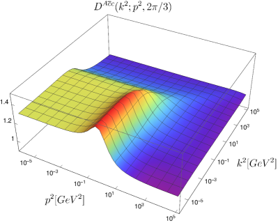
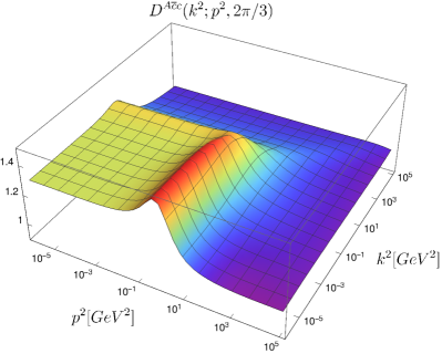
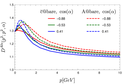
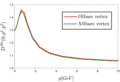
Lattice data for the ghost-gluon vertex in Coulomb gauge is not available. However, a qualitative comparison can be done with results form three-dimensional Yang-Mills theory [237]. A quantitative agreement can naturally not be achieved. Not only do the lattice results contain too many uncertainties, but also some basic differences exist. The foremost difference is expected in the UV. In Coulomb gauge, the ghost-gluon vertex possess an anomalous dimension while in three-dimensional Yang-Mills theory it approaches one rapidly. At small momenta, the shown results approach a value above one, whereas the lattice results are compatible with one. This is due to the lattice results supporting a solution of the decoupling type, whereas the results from the variational approach are of the scaling type. This difference in the IR behavior of the ghost-gluon vertex is known already from Landau gauge [176] and can be traced back to the fact that for the scaling type solution the integrals can have a nonzero contribution in the IR limit, whereas for decoupling they vanish in the IR. Despite these differences, it is instructive to compare the results to three-dimensional Yang-Mills theory due to the similar structure of the equations. And indeed the qualitative behavior of the ghost-gluon vertex is very similar in both cases. Also, in agreement with an IR analysis in three dimensions [171], no kinematic singularities are seen.
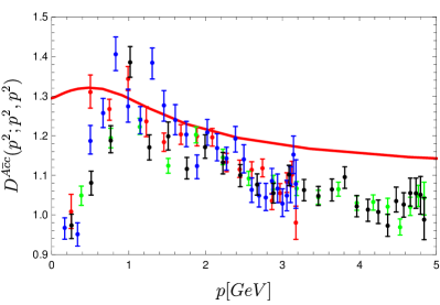
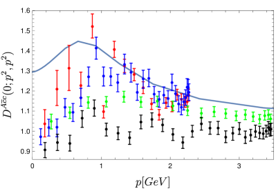
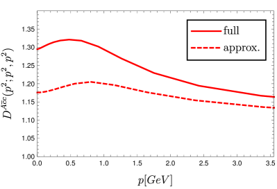
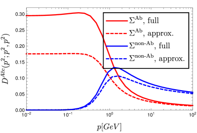
In Fig. 59 the effect of self-consistency is shown by comparing results for the -DSE to a semiperturbative calculation [148]. In that calculation, dressed propagators but bare ghost-gluon vertices were used. Clearly, solving the equation self-consistently increases the strength of the vertex. This is mostly due to the Abelian diagram. The non-Abelian diagram has in the -DSE only one ghost-gluon vertex so that backcoupling effects are not that large.
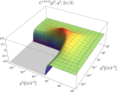
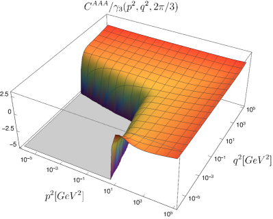
For the three-gluon vertex only the tree-level dressing is considered. It is then convenient to consider the dressing function divided by the variational kernel, . This quantity is more similar to the dressing function in other functional approaches, since the variational kernel plays here the role of the tree-level dressing. Thus, in some figues both and are shown. The calculation was done using a bare ghost-gluon vertex. It should also be noted that the appearance of the variational kernel instead of a bare vertex at the tree-level requires some additional steps in the renormalization procedure [178].
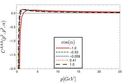
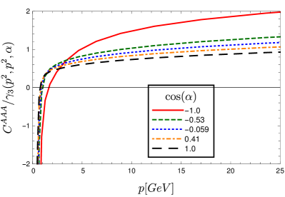
The kinematic dependence for the angle fixed to is shown in Fig. 60. The bump in the midmomentum regime appears due to the variational kernel and is not present in . The results are qualitatively indeed similar to calculations of the three-gluon vertex in three dimensions. However, here a larger angle dependence is observed, as shown in Fig. 61. In the IR, the vertex becomes negative and diverges with a power law, since the solution corresponds to a scaling type solution. The overall IR exponent of the full three-gluon vertex is , in agreement with the results obtained in Refs. [348, 144]. As in Landau gauge, the IR divergence is driven by the ghost triangle. The gluon triangle has only a small impact, as can be seen in Fig. 62, where the results from solving only with different subsets of diagrams are shown. From this figure, it is also evident that the swordfish diagrams do have a quantitative impact that should not be neglected. Due to the variational kernel of the four-gluon vertex, , one swordfish diagram also diverges as the ghost triangle with . This is in contrast to the Landau gauge, where all swordfish diagrams are IR suppressed compared to the ghost triangle. However, the coefficient of this power law is much smaller than that of the ghost triangle. It has only of the magnitude of the ghost triangle with the present truncation [178]. In general, the corresponding swordfish diagram does not have a large impact on the solution. Although its contribution is small, a reliable calculation of this diagram requires an increased precision compared to similar calculations in the Landau gauge [177, 176, 55].
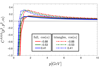
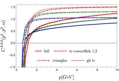
With the ghost triangle being the dominant part, the question of the importance of the ghost-gluon vertex arises. Fig. 63 shows the ghost triangle calculated with a bare and with a dressed ghost-gluon vertex. As can be expected, the ghost-gluon vertex shifts the zero crossing, but overall the effect is not very large and smaller than, e.g., the impact of the swordfish diagrams.
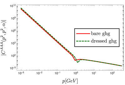
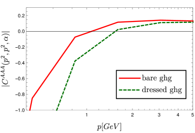
Results from the Hamiltonian approach in the Coulomb gauge including the ones presented here show that this gauge constitutes a reasonable alternative choice to the Landau gauge. With corresponding effort, calculations using similar sophisticated truncations as in the Landau gauge should be possible. Although the available results indicate a favorable answer, the question of the quantitative reliability of such calculations needs to be asked again. In any case, the Hamiltonian approach provides an interesting alternative perspective on the nonperturbative regime and can also be applied to full QCD [600, 601, 602, 603].
6 Conclusions
The investigation of the strong interaction has been an important topic in particle physics for the past decades, and we have not yet run out of problems to solve. Despite its deceptively simple form, the Lagrangian density of QCD still holds many secrets to be revealed. Functional methods constitute a promising approach in this endeavor. However, the fact that the exact equations have to be truncated is problematic as long as it is not known what the effect of a certain truncation is. By pushing truncations further and enlarging the systems of equations to be solved, the use of models can be reduced or in some cases even be eliminated. Such calculations demand a certain level of automatization for deriving and solving the equations which was made possible by tools that have been developed in recent years. Some of them were reviewed in Sec. 3.1.5.
The positive outcome of these efforts is increasing evidence that a self-contained and quantitative description of QCD from functional methods is achievable. To realize this, individual steps of understanding correlation functions and their mutual influence on each other must be taken and technical improvements must continue to be adopted. Within the last few years, some correlation functions were calculated for the first time nonperturbatively and we are learning to separate the important from the irrelevant facts. The emerging picture is promising, and although calculations are not getting easier, the potential benefit from establishing functional methods as a reliable nonperturbative method is motivating, for example, with regard to studies of the phase diagram of QCD.
The way to improve the reliability of functional equations seems simple: enlarge the truncation. However, it must be noted that this is not a plain brute force attack on the problem but involves also conceptual challenges. In particular, when replacing models with dynamic quantities new problems can surface and results might initially even get worse before the full picture is understood. The reason is simply that when models are used for unknown quantities, they provide a level of freedom that helps to overcome certain problems. Some of these problems may not even appear as such and one has to deal with them only once a certain level of truncation is reached. One example of the latter are the spurious divergences of the gluon propagator as discussed in detail in Sec. 4.2.1. Various methods to deal with them are known, but the results differ quantitatively. Only once we want quantitative results, care has to be taken how to subtract these divergences in order not to artificially influence the result. Another aspect that becomes relevant when one wants to obtain a self-contained solution is perturbative resummation. In this case, the problem lay dormant for a long time, because either no correct anomalous dimension was obtained, or the employed models guaranteed the self-consistency of the equation at the one-loop level. How to correctly realize resummation in DSEs is treated in Sec. 4.2.2.
To understand quantum field theory, functional equations and correlation functions better, it is often useful to consider variations of the physical theory, for example, by changing the number of dimensions. In the case of Yang-Mills theory, investigations of two and three dimensions proved to be helpful to scrutinize the structure of the solutions and the impact of different truncations as discussed in Sec. 4.3 and 4.4. Since in these dimensions the theory is finite, no anomalous running occurs. This simplifies the analysis. A consistent treatment of the anomalous running poses a challenge in four dimensions and links back to Sec. 4.2.2.
As argued in Sec. 4.1, the Landau gauge is the most widely adopted gauge for calculations with functional equations. To complete the picture, it is also useful to look at other gauges. Some examples were described in Sec. 5. Among them, in particular linear covariant gauges are receiving more attention lately. The reason is that their endpoint is the better understood Landau gauge and recently several problems related to the non-transverse gluon field have been addressed successfully.
For the future, the understanding of individual equations and insights into their interplay will be useful to unravel the nonperturbative regime of QCD. A particular challenge will be the study of its phase diagram. This is a field where functional equations can exert their advantages of being a continuum method without any inherent technical problems akin to the complex action problem of lattice QCD. Of course, nonvanishing temperature and density introduce another two layers of complexity. Having a good control over the vacuum results is a prerequisite to get on the right track to overcome also these problems.
Acknowledgments
During the last years I enjoyed many useful discussions and had the pleasure to learn from and collaborate with many colleagues. Among them I would like to thank in particular Reinhard Alkofer, Christian S. Fischer, Holger Gies, Jan M. Pawlowski, Lorenz von Smekal, and Andreas Wipf for their collaboration and their support.
For fruitful collaborations and helpful discussions I would like to thank Laurent Baulieu, Adrian L. Blum, Jens Braun, Davide Campagnari, Marcio A. L. Capri, Romain Contant, Anton K. Cyrol, David Dudal, Marcelo S. Guimaraes, Axel Maas, Mario Mitter, Hugo Reinhardt, Hèlios Sanchis Alepuz, Kai Schwenzer, Silvio P. Sorella, Nele Vandersickel, Richard Williams, Andreas Windisch, and Daniel Zwanziger.
In addition, discussions with Arlene Aguilar, Daniele Binosi, Gernot Eichmann, Leonard Fister, John Gracey, Markus Hopfer, Ernst-Michael Ilgenfritz, Christian Kellermann, Valentin Mader, Joannis Papavassiliou, Bernd-Jochen Schaefer, André Sternbeck, Ralf-Arno Tripolt, Selym Villalba-Chávez, Björn Wellegehausen, and Nicolas Wink were very helpful.
The most important thanks go to my family, to Birgit, Elisabeth and Katharina. Although they are only mentioned in this one line, they also contributed to this work in their own unique ways.
Funding
This research was supported by the Alexander von Humboldt foundation, the Helmholtz International Center for FAIR within the LOEWE program of the State of Hesse, the FWF (Austrian Science Fund) under Contract No. P 27380-N27 and the DFG (German Research Foundation) under Contract No. Fi970/11-1.
Technicalities
Appendix A Kernels
For reference some DSEs kernels are collected here. Two-loop kernels and vertex kernels are not given. Except for the ghost-gluon vertex, the kernels of which can be found in Ref. [176], they are too long to be useful in written form. To solve the corresponding DSEs, it is advised to create the required kernels with the help of some algebra program; see Sec. 3.1.5 for more information.
A.1 Landau gauge
For generality, the bare ghost-gluon vertex from general covariant gauges of Refs. [605, 606, 607, 608] is employed:
| (290) |
with . For most applications one can set . For the dressed vertex the dressing is added. For the gluon DSE the projector
| (291) |
is used. corresponds to the transverse projector which is typically chosen. This leads to the following expressions for the one-loop truncated propagator DSEs:
| (292) | ||||
| (293) |
There is no dependence on in the ghost equation, because its ghost-gluon vertex is contracted with a transverse projector, and the ghost-gluon vertex dressing was put explicitly. In the ghost loop of the gluon equation, the two structures of the bare vertex are contained in the kernel . The integral measure is defined as
| (294) |
The kernels are given by
| (295) | ||||
| (296) | ||||
| (297) | ||||
| (298) |
where , and .
A.2 Linear covariant gauges
The kernels for the gluon propagator DSE in linear covariant gauges, Eq. (5.1.2), are
| (299) | ||||
| (300) | ||||
| (301) | ||||
| (302) |
Appendix B Calculation of two-loop diagrams with a hard momentum cutoff
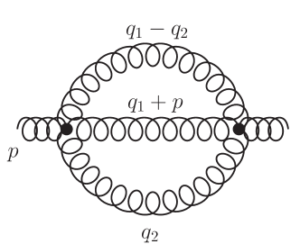
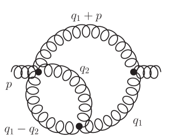
The calculation of a two-point two-loop integral of the type sunset or squint using a hard UV cutoff is described here. The generic integral reads
| (303) |
As can be seen in Fig. 64, the squint and sunset diagrams have similar integral structures except for the factor in the denominator. In actual perturbative calculations, the exponents are only one or two.
The external momentum is chosen to define the -direction, the loop momentum the --plane and the loop momentum the -- volume:
| (304) |
Two angles of and one angle of can be integrated trivially as they do not appear in any scalar products. The integral measure reduces then to
| (305) |
The integrals over the moduli of and have been rewritten to integrals over and .
In the one-loop case, the angle integrals have to be considered separately for and . The same applies here, only that now there are four different regions:
-
(I)
-
(II)
,
-
(III)
,
-
(IV)
,
For illustration, the angle integrals for , and are calculated in the following for .
Since for the angle integrals only the ratio of and is relevant, we introduce :
| (306) |
First, the integral over is performed. It should be noted that this reduces the power of by one:
| (307) |
is the integral over . To calculate it, the logarithm is split into a sum and the variable transformations and are employed:
| (308) |
Using the symmetry properties of the integrals, this expression can be rewritten to
| (309) |
and Eq. (B) becomes
| (310) |
where was plugged in. The final result is
| (311) |
is the unit step function. The case can be done in the same way, only that in this case one sets .
For the complete calculation of two-loop diagrams, many different are required. To keep calculations manageable, the calculation is automated. To this end, all required integrals are extracted from the expressions and precalculated analytically with Mathematica. Unfortunately, the correctness of the results is not guaranteed and different versions of Mathematica give different results. The trick to have correct results is quite simple, though. Every integral is checked numerically. If a wrong result is detected, the integral is recalculated after performing some simple rewritings like . The final list of results is converted into a list of simple replacement rules.
A tricky part is the required transformation of variables, as many different combinations appear. However, one can deal with that algorithmically and bring all expressions into the desired form before applying the rules. As a final test, all analytically derived results can be tested numerically at random points.
References
- [1] W. J. Marciano and H. Pagels, Quantum Chromodynamics: A Review, Phys.Rept. 36 (1978) 137.
- [2] N. Brambilla et al., QCD and Strongly Coupled Gauge Theories: Challenges and Perspectives, Eur. Phys. J. C74 no. 10, (2014) 2981, arXiv:1404.3723 [hep-ph].
- [3] D. J. Gross and F. Wilczek, Ultraviolet Behavior of Nonabelian Gauge Theories, Phys. Rev. Lett. 30 (1973) 1343–1346.
- [4] H. D. Politzer, Reliable Perturbative Results for Strong Interactions?, Phys. Rev. Lett. 30 (1973) 1346–1349.
- [5] T. Nash, T. Yamanouchi, D. Nease, and J. Sculli, A Search for Fractionally Charged Quarks Produced by 200-GeV and 300-GeV Proton - Nuclear Interactions, Phys. Rev. Lett. 32 (1974) 858–862.
- [6] D. Antreasyan, G. Cocconi, J. W. Cronin, H. J. Frisch, K. A. Olive, M. J. Shochet, L. Kluberg, J. Mueller, P. A. Piroue, and R. L. Sumner, Search for Quarks Produced with Large Transverse Momentum in 400-GeV Proton-Nucleus Collisions., Phys. Rev. Lett. 39 (1977) 513–515.
- [7] M. L. Stevenson, A search for massive, longlived, fractionally charged particles produced by 300-GeV protons, Phys. Rev. D20 (1979) 82.
- [8] CHARM Collaboration, F. Bergsma et al., Experimental Limits on the Production of Fractionally Charged Particles in Proton - Nucleus and Neutrino - Nucleus Collisions, Z. Phys. C24 (1984) 217.
- [9] R. L. Delgado, C. Hidalgo-Duque, and F. J. Llanes-Estrada, To What Extent is Gluon Confinement an Empirical Fact?, Few Body Syst. 54 (2013) 1705–1717, arXiv:1106.2462 [hep-ph].
- [10] R. Alkofer and J. Greensite, Quark Confinement: The Hard Problem of Hadron Physics, J. Phys. G34 (2007) S3, arXiv:hep-ph/0610365.
- [11] J. Greensite, The confinement problem in lattice gauge theory, Prog. Part. Nucl. Phys. 51 (2003) 1, arXiv:hep-lat/0301023.
- [12] K. G. Wilson, Confinement of Quarks, Phys. Rev. D10 (1974) 2445–2459.
- [13] G. Colangelo et al., Review of lattice results concerning low energy particle physics, Eur. Phys. J. C71 (2011) 1695, arXiv:1011.4408 [hep-lat].
- [14] C. Gattringer and C. B. Lang, Quantum chromodynamics on the lattice, Lect. Notes Phys. 788 (2010) 1–343.
- [15] Z. Fodor and C. Hoelbling, Light Hadron Masses from Lattice QCD, Rev. Mod. Phys. 84 (2012) 449, arXiv:1203.4789 [hep-lat].
- [16] S. Aoki et al., Review of lattice results concerning low-energy particle physics, Eur. Phys. J. C77 no. 2, (2017) 112, arXiv:1607.00299 [hep-lat].
- [17] S. Borsanyi, Z. Fodor, C. Hoelbling, S. D. Katz, S. Krieg, and K. K. Szabo, Full result for the QCD equation of state with 2+1 flavors, Phys. Lett. B730 (2014) 99–104, arXiv:1309.5258 [hep-lat].
- [18] HotQCD Collaboration, A. Bazavov et al., Equation of state in ( 2+1 )-flavor QCD, Phys. Rev. D90 (2014) 094503, arXiv:1407.6387 [hep-lat].
- [19] P. de Forcrand, Simulating QCD at finite density, PoS LAT2009 (2009) 010, arXiv:1005.0539 [hep-lat].
- [20] R. Alkofer and L. von Smekal, The infrared behavior of QCD Green’s functions: Confinement, dynamical symmetry breaking, and hadrons as relativistic bound states, Phys. Rept. 353 (2001) 281, arXiv:hep-ph/0007355.
- [21] A. Bashir, L. Chang, I. C. Cloet, B. El-Bennich, Y.-X. Liu, C. Roberts, C. D., and P. Tandy, Collective perspective on advances in Dyson-Schwinger Equation QCD, Commun.Theor.Phys. 58 (2012) 79–134, arXiv:1201.3366 [nucl-th].
- [22] G. Eichmann, H. Sanchis-Alepuz, R. Williams, R. Alkofer, and C. S. Fischer, Baryons as relativistic three-quark bound states, Prog. Part. Nucl. Phys. 91 (2016) 1–100, arXiv:1606.09602 [hep-ph].
- [23] M. Q. Huber, C. S. Fischer, and H. Sanchis-Alepuz, Spectrum of scalar and pseudoscalar glueballs from functional methods, arXiv:2004.00415 [hep-ph].
- [24] M. Q. Huber, Correlation functions of Landau gauge Yang-Mills theory, arXiv:2003.13703 [hep-ph].
- [25] H. Fritzsch, M. Gell-Mann, and H. Leutwyler, Advantages of the Color Octet Gluon Picture, Phys. Lett. B47 (1973) 365–368.
- [26] C.-N. Yang and R. L. Mills, Conservation of isotopic spin and isotopic gauge invariance, Phys. Rev. 96 (1954) 191–195.
- [27] L. D. Faddeev and V. N. Popov, Feynman diagrams for the Yang-Mills field, Phys. Lett. B25 (1967) 29–30.
- [28] V. Gribov, Quantization of Nonabelian Gauge Theories, Nucl.Phys. B139 (1978) 1.
- [29] I. M. Singer, Some Remarks on the Gribov Ambiguity, Commun. Math. Phys. 60 (1978) 7–12.
- [30] H. Huffel and D. Markovic, Perturbative Yang–Mills theory without Faddeev–Popov ghost fields, Phys. Lett. B780 (2018) 418–421, arXiv:1712.10302 [hep-th].
- [31] C. Becchi, A. Rouet, and R. Stora, Renormalization of Gauge Theories, Annals Phys. 98 (1976) 287–321.
- [32] C. Becchi, A. Rouet, and R. Stora, Renormalization of the Abelian Higgs-Kibble Model, Commun. Math. Phys. 42 (1975) 127–162.
- [33] I. V. Tyutin, Gauge Invariance in Field Theory and Statistical Physics in Operator Formalism, arXiv:0812.0580 [hep-th].
- [34] T. Kugo and I. Ojima, Local Covariant Operator Formalism of Nonabelian Gauge Theories and Quark Confinement Problem, Prog. Theor. Phys. Suppl. 66 (1979) 1.
- [35] O. Piguet and S. P. Sorella, Algebraic renormalization: Perturbative renormalization, symmetries and anomalies, Lect. Notes Phys. M28 (1995) 1–134.
- [36] N. Nakanishi, Indefinite metric quantum field theory, Prog. Theor. Phys. Suppl. 51 (1972) 1–95.
- [37] B. Lautrup, Canonical quantum electrodynamcis in covariant gauges, Kong. Dan. Vid. Sel. Mat. Fys. Med. 35 no. 11, (1967) .
- [38] T. Kugo and S. Uehara, General Procedure of Gauge Fixing Based on BRS Invariance Principle, Nucl. Phys. B197 (1982) 378–384.
- [39] M. C. M. Wright, Green function or Green’s function?, Nature Physics 2(10) (2006) 646.
- [40] G. Eichmann, C. S. Fischer, and W. Heupel, Four-point functions and the permutation group S4, Phys. Rev. D92 no. 5, (2015) 056006, arXiv:1505.06336 [hep-ph].
- [41] A. Salam, Renormalizable electrodynamics of vector mesons, Phys. Rev. 130 (1963) 1287–1290.
- [42] A. Salam and R. Delbourgo, Renormalizable electrodynamics of scalar and vector mesons. II, Phys. Rev. 135 (1964) B1398–B1427.
- [43] R. Delbourgo and P. C. West, A Gauge Covariant Approximation to Quantum Electrodynamics, J. Phys. A 10 (1977) 1049.
- [44] R. Delbourgo and P. C. West, Infrared Behavior of a Gauge Covariant Approximation, Phys. Lett. B 72 (1977) 96–98.
- [45] A. C. Aguilar and J. Papavassiliou, Chiral symmetry breaking with lattice propagators, Phys. Rev. D83 (2011) 014013, arXiv:1010.5815 [hep-ph].
- [46] E. Rojas, J. de Melo, B. El-Bennich, O. Oliveira, and T. Frederico, On the Quark-Gluon Vertex and Quark-Ghost Kernel: combining Lattice Simulations with Dyson-Schwinger equations, JHEP 1310 (2013) 193, arXiv:1306.3022 [hep-ph].
- [47] A. Aguilar, J. Cardona, M. Ferreira, and J. Papavassiliou, Quark gap equation with non-abelian Ball-Chiu vertex, Phys. Rev. D 98 no. 1, (2018) 014002, arXiv:1804.04229 [hep-ph].
- [48] A. C. Aguilar, D. Binosi, D. Ibañez, and J. Papavassiliou, New method for determining the quark-gluon vertex, Phys. Rev. D90 no. 6, (2014) 065027, arXiv:1405.3506 [hep-ph].
- [49] A. C. Aguilar, J. C. Cardona, M. N. Ferreira, and J. Papavassiliou, Non-Abelian Ball-Chiu vertex for arbitrary Euclidean momenta, Phys. Rev. D96 no. 1, (2017) 014029, arXiv:1610.06158 [hep-ph].
- [50] O. Oliveira, T. Frederico, W. de Paula, and J. de Melo, Exploring the Quark-Gluon Vertex with Slavnov-Taylor Identities and Lattice Simulations, Eur. Phys. J. C 78 no. 7, (2018) 553, arXiv:1807.00675 [hep-ph].
- [51] A. Aguilar, M. Ferreira, C. Figueiredo, and J. Papavassiliou, Nonperturbative structure of the ghost-gluon kernel, Phys. Rev. D 99 no. 3, (2019) 034026, arXiv:1811.08961 [hep-ph].
- [52] A. Aguilar, M. Ferreira, C. Figueiredo, and J. Papavassiliou, Nonperturbative Ball-Chiu construction of the three-gluon vertex, Phys. Rev. D 99 no. 9, (2019) 094010, arXiv:1903.01184 [hep-ph].
- [53] C. S. Fischer, A. Maas, and J. M. Pawlowski, On the infrared behavior of Landau gauge Yang-Mills theory, Annals Phys. 324 (2009) 2408–2437, arXiv:0810.1987 [hep-ph].
- [54] M. Carrington and Y. Guo, Techniques for n-Particle Irreducible Effective Theories, Phys.Rev. D83 (2011) 016006, arXiv:1010.2978 [hep-ph].
- [55] G. Eichmann, R. Williams, R. Alkofer, and M. Vujinovic, The three-gluon vertex in Landau gauge, Phys.Rev. D89 (2014) 105014, arXiv:1402.1365 [hep-ph].
- [56] C. Lerche and L. von Smekal, On the infrared exponent for gluon and ghost propagation in Landau gauge QCD, Phys.Rev. D65 (2002) 125006, arXiv:hep-ph/0202194.
- [57] N. V. Smolyakov, Furry Theorem for Nonabelian Gauge Lagrangians, Theor. Math. Phys. 50 (1982) 225–228. [Teor. Mat. Fiz.50,344(1982)],
- [58] R. Peccei, Discrete and global symmetries in particle physics, Lect. Notes Phys. 521 (1999) 1–50, arXiv:hep-ph/9807516.
- [59] A. L. Blum, R. Alkofer, M. Q. Huber, and A. Windisch, Unquenching the three-gluon vertex: A status report, Acta Phys. Polon. Supp. 8 no. 2, (2015) 321, arXiv:1506.04275 [hep-ph].
- [60] J. S. Ball and T.-W. Chiu, Analytic Properties of the Vertex Function in Gauge Theories. 1., Phys. Rev. D22 (1980) 2542.
- [61] M. Hopfer, A. Windisch, and R. Alkofer, The Quark-Gluon Vertex in Landau gauge QCD, PoS ConfinementX (2012) 073, arXiv:1301.3672 [hep-ph].
- [62] R. Williams, The quark-gluon vertex in Landau gauge bound-state studies, Eur. Phys. J. A51 no. 5, (2015) 57, arXiv:1404.2545 [hep-ph].
- [63] M. Hopfer, Gauge theories: QCD & beyond. PhD thesis, Graz U., 2014. http://unipub.uni-graz.at/obvugrhs/content/titleinfo/269085.
- [64] A. Windisch, Features of strong quark correlations at vanishing and non-vanishing density. PhD thesis, Graz U., 2014. http://unipub.uni-graz.at/obvugrhs/content/titleinfo/242468.
- [65] M. Mitter, J. M. Pawlowski, and N. Strodthoff, Chiral symmetry breaking in continuum QCD, Phys. Rev. D91 (2015) 054035, arXiv:1411.7978 [hep-ph].
- [66] R. Williams, C. S. Fischer, and W. Heupel, Light mesons in QCD and unquenching effects from the 3PI effective action, Phys. Rev. D93 no. 3, (2016) 034026, arXiv:1512.00455 [hep-ph].
- [67] A. K. Cyrol, M. Mitter, J. M. Pawlowski, and N. Strodthoff, Nonperturbative quark, gluon, and meson correlators of unquenched QCD, Phys. Rev. D97 no. 5, (2018) 054006, arXiv:1706.06326 [hep-ph].
- [68] P. Pascual and R. Tarrach, Slavnov-Taylor Identities in Weinberg’s Renormalization Scheme, Nucl.Phys. B174 (1980) 123.
- [69] L. Driesen, J. Fromm, J. Kuhrs, and M. Stingl, Extended iterative scheme for QCD: Three point vertices, Eur. Phys. J. A4 (1999) 381–400, arXiv:hep-th/9808152 [hep-th].
- [70] L. Driesen and M. Stingl, Extended iterative scheme for QCD: The Four gluon vertex, Eur.Phys.J. A4 (1999) 401–419, arXiv:hep-th/9808155 [hep-th].
- [71] A. K. Cyrol, M. Q. Huber, and L. von Smekal, A Dyson–Schwinger study of the four-gluon vertex, Eur. Phys. J. C75 (2015) 102, arXiv:1408.5409 [hep-ph].
- [72] F. J. Dyson, The S matrix in quantum electrodynamics, Phys. Rev. 75 (1949) 1736–1755.
- [73] J. S. Schwinger, On the Green’s functions of quantized fields. 1, Proc. Nat. Acad. Sci. 37 (1951) 452–455.
- [74] J. S. Schwinger, On the Green’s functions of quantized fields. 2, Proc. Nat. Acad. Sci. 37 (1951) 455–459.
- [75] J. M. Cornwall, Dynamical Mass Generation in Continuum QCD, Phys. Rev. D26 (1982) 1453.
- [76] J. M. Cornwall and J. Papavassiliou, Gauge Invariant Three Gluon Vertex in QCD, Phys. Rev. D40 (1989) 3474.
- [77] D. Binosi and J. Papavassiliou, The Pinch technique to all orders, Phys. Rev. D66 (2002) 111901, arXiv:hep-ph/0208189 [hep-ph].
- [78] D. Binosi and J. Papavassiliou, Pinch technique selfenergies and vertices to all orders in perturbation theory, J. Phys. G30 (2004) 203, arXiv:hep-ph/0301096 [hep-ph].
- [79] L. F. Abbott, The Background Field Method Beyond One Loop, Nucl. Phys. B185 (1981) 189–203.
- [80] L. F. Abbott, Introduction to the Background Field Method, Acta Phys. Polon. B13 (1982) 33.
- [81] A. C. Aguilar and J. Papavassiliou, Gluon mass generation in the PT-BFM scheme, JHEP 0612 (2006) 012, arXiv:hep-ph/0610040 [hep-ph].
- [82] D. Binosi and J. Papavassiliou, Gauge-invariant truncation scheme for the Schwinger-Dyson equations of QCD, Phys. Rev. D77 (2008) 061702, arXiv:0712.2707 [hep-ph].
- [83] D. Binosi and J. Papavassiliou, New Schwinger-Dyson equations for non-Abelian gauge theories, JHEP 11 (2008) 063, arXiv:0805.3994 [hep-ph].
- [84] D. Binosi and J. Papavassiliou, Pinch Technique: Theory and Applications, Phys. Rept. 479 (2009) 1–152, arXiv:0909.2536 [hep-ph].
- [85] A. Aguilar, D. Binosi, and J. Papavassiliou, Gluon and ghost propagators in the Landau gauge: Deriving lattice results from Schwinger-Dyson equations, Phys.Rev. D78 (2008) 025010, arXiv:0802.1870 [hep-ph].
- [86] A. C. Aguilar and J. Papavassiliou, Gluon mass generation without seagull divergences, Phys.Rev. D81 (2010) 034003, arXiv:0910.4142 [hep-ph].
- [87] J. Rodriguez-Quintero, On the massive gluon propagator, the PT-BFM scheme and the low-momentum behaviour of decoupling and scaling DSE solutions, JHEP 01 (2011) 105, arXiv:1005.4598 [hep-ph].
- [88] A. Aguilar, D. Binosi, and J. Papavassiliou, The dynamical equation of the effective gluon mass, Phys.Rev. D84 (2011) 085026, arXiv:1107.3968 [hep-ph].
- [89] A. Aguilar, D. Binosi, and J. Papavassiliou, Gluon mass through ghost synergy, JHEP 1201 (2012) 050, arXiv:1108.5989 [hep-ph].
- [90] D. Binosi, D. Ibáñez, and J. Papavassiliou, The all-order equation of the effective gluon mass, arXiv:1208.1451 [hep-ph].
- [91] A. Aguilar, D. Binosi, D. Ibáñez, and J. Papavassiliou, Effects of divergent ghost loops on the Green’s functions of QCD, Phys.Rev. D89 (2014) 085008, arXiv:1312.1212 [hep-ph].
- [92] A. C. Aguilar, D. Binosi, and J. Papavassiliou, Schwinger mechanism in linear covariant gauges, Phys. Rev. D95 no. 3, (2017) 034017, arXiv:1611.02096 [hep-ph].
- [93] A. Aguilar, M. Ferreira, C. Figueiredo, and J. Papavassiliou, Gluon mass scale through nonlinearities and vertex interplay, Phys. Rev. D 100 no. 9, (2019) 094039, arXiv:1909.09826 [hep-ph].
- [94] A. Aguilar, F. De Soto, M. Ferreira, J. Papavassiliou, J. Rodríguez-Quintero, and S. Zafeiropoulos, Gluon propagator and three-gluon vertex with dynamical quarks, Eur. Phys. J. C 80 no. 2, (2020) 154, arXiv:1912.12086 [hep-ph].
- [95] T. Pfeffer and L. Pollet, A stochastic root finding approach: the homotopy analysis method applied to Dyson–Schwinger equations, New J. Phys. 19 no. 4, (2017) 043005, arXiv:1701.02680 [cond-mat.stat-mech].
- [96] T. Pfeffer and L. Pollet, Full and unbiased solution of the Dyson-Schwinger equation in the functional integro-differential representation, arXiv:1803.00961 [cond-mat.stat-mech].
- [97] J. M. Cornwall, R. Jackiw, and E. Tomboulis, Effective Action for Composite Operators, Phys. Rev. D10 (1974) 2428–2445.
- [98] J. Berges, n-PI effective action techniques for gauge theories, Phys. Rev. D70 (2004) 105010, arXiv:hep-ph/0401172.
- [99] R. Jackiw, Functional evaluation of the effective potential, Phys. Rev. D9 (1974) 1686.
- [100] S. Diehl, S. Floerchinger, H. Gies, J. M. Pawlowski, and C. Wetterich, Functional renormalization group approach to the BCS-BEC crossover, Annalen Phys. 522 (2010) 615–656, arXiv:0907.2193 [cond-mat.quant-gas].
- [101] S. Diehl, H. Gies, J. M. Pawlowski, and C. Wetterich, Flow Equations for the BCS-BEC Crossover, Phys. Rev. A76 (2007) 021602, arXiv:cond-mat/0701198.
- [102] I. Boettcher, J. M. Pawlowski, and S. Diehl, Ultracold atoms and the Functional Renormalization Group, Nucl. Phys. Proc. Suppl. 228 (2012) 63–135, arXiv:1204.4394 [cond-mat.quant-gas].
- [103] H. Gies, F. Synatschke, and A. Wipf, Supersymmetry breaking as a quantum phase transition, Phys. Rev. D80 (2009) 101701, arXiv:0906.5492 [hep-th].
- [104] F. Synatschke, J. Braun, and A. Wipf, N=1 Wess Zumino Model in d=3 at zero and finite temperature, Phys. Rev. D81 (2010) 125001, arXiv:1001.2399 [hep-th].
- [105] F. Synatschke, H. Gies, and A. Wipf, Phase Diagram and Fixed-Point Structure of two dimensional N=1 Wess-Zumino Models, Phys. Rev. D80 (2009) 085007, arXiv:0907.4229 [hep-th].
- [106] D. F. Litim, M. C. Mastaler, F. Synatschke-Czerwonka, and A. Wipf, Critical behavior of supersymmetric O(N) models in the large-N limit, Phys. Rev. D84 (2011) 125009, arXiv:1107.3011 [hep-th].
- [107] M. Heilmann, D. F. Litim, F. Synatschke-Czerwonka, and A. Wipf, Phases of supersymmetric O(N) theories, Phys. Rev. D86 (2012) 105006, arXiv:1208.5389 [hep-th].
- [108] E. Manrique and M. Reuter, Bare vs. Effective Fixed Point Action in Asymptotic Safety: The Reconstruction Problem, arXiv:0905.4220 [hep-th]. Talk given at International Workshop on Continuum and Lattice Approaches to Quantum Gravity, Brighton, United Kingdom, 17-19 Sep 08.,
- [109] M. Reuter, Nonperturbative Evolution Equation for Quantum Gravity, Phys. Rev. D57 (1998) 971–985, arXiv:hep-th/9605030.
- [110] M. Reuter and F. Saueressig, Renormalization group flow of quantum gravity in the Einstein-Hilbert truncation, Phys. Rev. D65 (2002) 065016, arXiv:hep-th/0110054.
- [111] A. Codello, R. Percacci, and C. Rahmede, Ultraviolet properties of f(R)-gravity, Int. J. Mod. Phys. A23 (2008) 143–150, arXiv:0705.1769 [hep-th].
- [112] A. Eichhorn and H. Gies, Ghost anomalous dimension in asymptotically safe quantum gravity, Phys. Rev. D81 (2010) 104010, arXiv:1001.5033 [hep-th].
- [113] A. Eichhorn, H. Gies, and M. M. Scherer, Asymptotically free scalar curvature-ghost coupling in Quantum Einstein Gravity, Phys. Rev. D80 (2009) 104003, arXiv:0907.1828 [hep-th].
- [114] D. F. Litim, Renormalisation group and the Planck scale, Phil. Trans. Roy. Soc. Lond. A369 (2011) 2759–2778, arXiv:1102.4624 [hep-th].
- [115] S. Folkerts, D. F. Litim, and J. M. Pawlowski, Asymptotic freedom of Yang-Mills theory with gravity, Phys. Lett. B709 (2012) 234–241, arXiv:1101.5552 [hep-th].
- [116] T. Denz, J. M. Pawlowski, and M. Reichert, Towards apparent convergence in asymptotically safe quantum gravity, arXiv:1612.07315 [hep-th].
- [117] H. Gies, B. Knorr, S. Lippoldt, and F. Saueressig, Gravitational Two-Loop Counterterm Is Asymptotically Safe, Phys. Rev. Lett. 116 no. 21, (2016) 211302, arXiv:1601.01800 [hep-th].
- [118] A. Bonanno and F. Saueressig, Asymptotically safe cosmology – A status report, Comptes Rendus Physique 18 (2017) 254–264, arXiv:1702.04137 [hep-th].
- [119] A. Platania and F. Saueressig, Functional Renormalization Group flows on Friedman-Lemaître-Robertson-Walker backgrounds, arXiv:1710.01972 [hep-th].
- [120] H. Gies, C. Gneiting, and R. Sondenheimer, Higgs Mass Bounds from Renormalization Flow for a simple Yukawa model, Phys. Rev. D89 no. 4, (2014) 045012, arXiv:1308.5075 [hep-ph].
- [121] H. Gies and R. Sondenheimer, Higgs Mass Bounds from Renormalization Flow for a Higgs-top-bottom model, Eur. Phys. J. C75 no. 2, (2015) 68, arXiv:1407.8124 [hep-ph].
- [122] J. Borchardt, H. Gies, and R. Sondenheimer, Global flow of the Higgs potential in a Yukawa model, Eur. Phys. J. C76 no. 8, (2016) 472, arXiv:1603.05861 [hep-ph].
- [123] H. Gies, R. Sondenheimer, and M. Warschinke, Impact of generalized Yukawa interactions on the lower Higgs mass bound, Eur. Phys. J. C77 no. 11, (2017) 743, arXiv:1707.04394 [hep-ph].
- [124] B.-J. Schaefer and J. Wambach, Renormalization group approach towards the QCD phase diagram, Phys. Part. Nucl. 39 (2008) 1025–1032, arXiv:hep-ph/0611191.
- [125] B.-J. Schaefer and J. Wambach, Susceptibilities near the QCD (tri)critical point, Phys. Rev. D75 (2007) 085015, arXiv:hep-ph/0603256.
- [126] J. Braun, H. Gies, and J. M. Pawlowski, Quark Confinement from Color Confinement, Phys. Lett. B684 (2010) 262–267, arXiv:0708.2413 [hep-th].
- [127] B.-J. Schaefer and M. Wagner, The three-flavor chiral phase structure in hot and dense QCD matter, Phys. Rev. D79 (2009) 014018, arXiv:0808.1491 [hep-ph].
- [128] J. Braun, L. M. Haas, F. Marhauser, and J. M. Pawlowski, Phase Structure of Two-Flavor QCD at Finite Chemical Potential, Phys. Rev. Lett. 106 (2011) 022002, arXiv:0908.0008 [hep-ph].
- [129] T. K. Herbst, J. M. Pawlowski, and B.-J. Schaefer, The phase structure of the Polyakov–quark-meson model beyond mean field, Phys. Lett. B696 (2011) 58–67, arXiv:1008.0081 [hep-ph].
- [130] J. M. Pawlowski, The QCD phase diagram: Results and challenges, AIP Conf.Proc. 1343 (2011) 75–80, arXiv:1012.5075 [hep-ph].
- [131] L. Fister and J. M. Pawlowski, Yang-Mills correlation functions at finite temperature, arXiv:1112.5440 [hep-ph].
- [132] L. M. Haas, R. Stiele, J. Braun, J. M. Pawlowski, and J. Schaffner-Bielich, Improved Polyakov-loop potential for effective models from functional calculations, Phys.Rev. D87 (2013) 076004, arXiv:1302.1993 [hep-ph].
- [133] T. K. Herbst, M. Mitter, J. M. Pawlowski, B.-J. Schaefer, and R. Stiele, Thermodynamics of QCD at vanishing density, Phys.Lett. B731 (2014) 248–256, arXiv:1308.3621 [hep-ph].
- [134] M. Haas, L. Fister, and J. M. Pawlowski, Gluon spectral functions and transport coefficients in Yang–Mills theory, Phys. Rev. D90 (2014) 091501, arXiv:1308.4960 [hep-ph].
- [135] R.-A. Tripolt, L. von Smekal, and J. Wambach, Flow equations for spectral functions at finite external momenta, Phys. Rev. D90 no. 7, (2014) 074031, arXiv:1408.3512 [hep-ph].
- [136] N. Christiansen, M. Haas, J. M. Pawlowski, and N. Strodthoff, Transport Coefficients in Yang–Mills Theory and QCD, Phys. Rev. Lett. 115 no. 11, (2015) 112002, arXiv:1411.7986 [hep-ph].
- [137] A. K. Cyrol, M. Mitter, J. M. Pawlowski, and N. Strodthoff, Nonperturbative finite-temperature Yang-Mills theory, Phys. Rev. D97 no. 5, (2018) 054015, arXiv:1708.03482 [hep-ph].
- [138] J. Berges, N. Tetradis, and C. Wetterich, Non-perturbative renormalization flow in quantum field theory and statistical physics, Phys. Rept. 363 (2002) 223–386, arXiv:hep-ph/0005122.
- [139] J. M. Pawlowski, Aspects of the functional renormalisation group, Annals Phys. 322 (2007) 2831–2915, arXiv:hep-th/0512261.
- [140] H. Gies, Introduction to the functional RG and applications to gauge theories, Lect.Notes Phys. 852 (2012) 287–348, arXiv:hep-ph/0611146 [hep-ph].
- [141] C. Wetterich, Exact evolution equation for the effective potential, Phys. Lett. B301 (1993) 90–94.
- [142] M. Quandt, H. Reinhardt, and J. Heffner, Covariant variational approach to Yang-Mills theory, Phys. Rev. D89 no. 6, (2014) 065037, arXiv:1310.5950 [hep-th].
- [143] H. Reinhardt and W. Schleifenbaum, Hamiltonian Approach to 1+1 dimensional Yang-Mills theory in Coulomb gauge, Annals Phys. 324 (2009) 735–786, arXiv:0809.1764 [hep-th].
- [144] D. R. Campagnari and H. Reinhardt, Non-Gaussian wave functionals in Coulomb gauge Yang–Mills theory, Phys.Rev. D82 (2010) 105021, arXiv:1009.4599 [hep-th].
- [145] D. Schutte, Nonperturbative many body techniques applied to a Yang-Mills field theory, Phys. Rev. D31 (1985) 810–821.
- [146] A. P. Szczepaniak and E. S. Swanson, Coulomb gauge QCD, confinement, and the constituent representation, Phys. Rev. D65 (2002) 025012, arXiv:hep-ph/0107078 [hep-ph].
- [147] C. Feuchter and H. Reinhardt, Variational solution of the Yang-Mills Schrodinger equation in Coulomb gauge, Phys.Rev. D70 (2004) 105021, arXiv:hep-th/0408236 [hep-th].
- [148] D. R. Campagnari and H. Reinhardt, The ghost-gluon vertex in Hamiltonian Yang-Mills theory in Coulomb gauge, Phys.Lett. B707 (2012) 216–220, arXiv:1111.5476 [hep-th].
- [149] R. Alkofer, M. Q. Huber, and K. Schwenzer, Algorithmic derivation of Dyson-Schwinger Equations, Comput. Phys. Commun. 180 (2009) 965–976, arXiv:0808.2939 [hep-th].
- [150] S. Wolfram, The Mathematica Book. Wolfram Media and Cambridge University Press, 2004.
- [151] M. Q. Huber, K. Schwenzer, and R. Alkofer, On the infrared scaling solution of SU(N) Yang-Mills theories in the maximally Abelian gauge, Eur. Phys. J. C68 (2010) 581–600, arXiv:0904.1873 [hep-th].
- [152] M. Q. Huber, R. Alkofer, and S. P. Sorella, Infrared analysis of Dyson-Schwinger equations taking into account the Gribov horizon in Landau gauge, Phys. Rev. D81 (2010) 065003, arXiv:0910.5604 [hep-th].
- [153] T. van Ritbergen, A. N. Schellekens, and J. A. M. Vermaseren, Group theory factors for Feynman diagrams, Int. J. Mod. Phys. A14 (1999) 41–96, arXiv:hep-ph/9802376.
- [154] J. A. M. Vermaseren, New features of FORM, arXiv:math-ph/0010025.
- [155] J. Kuipers, T. Ueda, J. A. M. Vermaseren, and J. Vollinga, FORM version 4.0, Comput. Phys. Commun. 184 (2013) 1453–1467, arXiv:1203.6543 [cs.SC].
- [156] J. Kuipers, T. Ueda, and J. A. M. Vermaseren, Code Optimization in FORM, Comput. Phys. Commun. 189 (2015) 1–19, arXiv:1310.7007 [cs.SC].
- [157] B. Ruijl, T. Ueda, and J. Vermaseren, FORM version 4.2, arXiv:1707.06453 [hep-ph].
- [158] R. Mertig, M. Bohm, and A. Denner, FEYN CALC: Computer algebraic calculation of Feynman amplitudes, Comput. Phys. Commun. 64 (1991) 345–359.
- [159] V. Shtabovenko, R. Mertig, and F. Orellana, New Developments in FeynCalc 9.0, Comput. Phys. Commun. 207 (2016) 432–444, arXiv:1601.01167 [hep-ph].
- [160] V. Shtabovenko, FeynHelpers: Connecting FeynCalc to FIRE and Package-X, Comput. Phys. Commun. 218 (2017) 48–65, arXiv:1611.06793 [physics.comp-ph].
- [161] M. Wiebusch, HEPMath 1.4: A mathematica package for semi-automatic computations in high energy physics, Comput. Phys. Commun. 195 (2015) 172–190, arXiv:1412.6102 [hep-ph].
- [162] M. Jamin and M. E. Lautenbacher, TRACER: Version 1.1: A Mathematica package for gamma algebra in arbitrary dimensions, Comput. Phys. Commun. 74 (1993) 265–288.
- [163] A. K. Cyrol, M. Mitter, and N. Strodthoff, FormTracer - A Mathematica Tracing Package Using FORM, Comput. Phys. Commun. 219 (2017) 346–352, arXiv:1610.09331 [hep-ph].
- [164] M. Q. Huber and J. Braun, Algorithmic derivation of functional renormalization group equations and Dyson-Schwinger equations, Comput.Phys.Commun. 183 (2012) 1290–1320, arXiv:1102.5307 [hep-th].
- [165] J. Braun, M. Leonhardt, and M. Pospiech, Fierz-complete NJL model study: Fixed points and phase structure at finite temperature and density, Phys. Rev. D96 no. 7, (2017) 076003, arXiv:1705.00074 [hep-ph].
- [166] J. Braun, M. Leonhardt, and M. Pospiech, Fierz-complete NJL model study. II. Toward the fixed-point and phase structure of hot and dense two-flavor QCD, Phys. Rev. D97 no. 7, (2018) 076010, arXiv:1801.08338 [hep-ph].
- [167] R. Alkofer, A. Maas, W. A. Mian, M. Mitter, J. París-López, J. M. Pawlowski, and N. Wink, Bound state properties from the functional renormalization group, Phys. Rev. D99 no. 5, (2019) 054029, arXiv:1810.07955 [hep-ph].
- [168] J. Eser, F. Divotgey, M. Mitter, and D. H. Rischke, Low-energy limit of the quark-meson model from the functional renormalization group approach, Phys. Rev. D98 no. 1, (2018) 014024, arXiv:1804.01787 [hep-ph].
- [169] J. Braun, M. Leonhardt, and M. Pospiech, Fierz-complete NJL model study III: Emergence from quark-gluon dynamics, arXiv:1909.06298 [hep-ph].
- [170] F. Divotgey, J. Eser, and M. Mitter, Dynamical generation of low-energy couplings from quark-meson fluctuations, Phys. Rev. D99 no. 5, (2019) 054023, arXiv:1901.02472 [hep-ph].
- [171] R. Alkofer, M. Q. Huber, and K. Schwenzer, Infrared Behavior of Three-Point Functions in Landau Gauge Yang-Mills Theory, Eur. Phys. J. C62 (2009) 761–781, arXiv:0812.4045 [hep-ph].
- [172] L. Fister, R. Alkofer, and K. Schwenzer, On the Infrared Behavior of Landau Gauge Yang-Mills Theory with a Fundamentally Charged Scalar Field, Phys. Lett. B688 (2010) 237–243, arXiv:1003.1668 [hep-th].
- [173] V. Macher, A. Maas, and R. Alkofer, A Study of the Influence of the Gauge Group on the Dyson-Schwinger Equations for Scalar-Yang-Mills Systems, Int. J. Mod. Phys. A27 (2012) 1250098, arXiv:1106.5381 [hep-ph].
- [174] N. Alkofer and R. Alkofer, Features of ghost-gluon and ghost-quark bound states related to BRST quartets, Phys. Lett. B702 (2011) 158–163, arXiv:1102.2753 [hep-th].
- [175] M. Q. Huber, A. Maas, and L. von Smekal, Two- and three-point functions in two-dimensional Landau-gauge Yang-Mills theory: Continuum results, JHEP 1211 (2012) 035, arXiv:1207.0222 [hep-th].
- [176] M. Q. Huber and L. von Smekal, On the influence of three-point functions on the propagators of Landau gauge Yang-Mills theory, JHEP 1304 (2013) 149, arXiv:1211.6092 [hep-th].
- [177] A. Blum, M. Q. Huber, M. Mitter, and L. von Smekal, Gluonic three-point correlations in pure Landau gauge QCD, Phys. Rev. D 89 (2014) 061703(R), arXiv:1401.0713 [hep-ph].
- [178] M. Q. Huber, D. R. Campagnari, and H. Reinhardt, Vertex functions of Coulomb gauge Yang–Mills theory, Phys.Rev. D91 no. 2, (2015) 025014, arXiv:1410.4766 [hep-ph].
- [179] M. Q. Huber and L. von Smekal, Spurious divergences in Dyson-Schwinger equations, JHEP 1406 (2014) 015, arXiv:1404.3642 [hep-ph].
- [180] J. Braun, L. Fister, J. M. Pawlowski, and F. Rennecke, From Quarks and Gluons to Hadrons: Chiral Symmetry Breaking in Dynamical QCD, arXiv:1412.1045 [hep-ph].
- [181] F. Rennecke, Vacuum structure of vector mesons in QCD, Phys. Rev. D92 no. 7, (2015) 076012, arXiv:1504.03585 [hep-ph].
- [182] M. Q. Huber, Gluon and ghost propagators in linear covariant gauges, Phys. Rev. D91 no. 8, (2015) 085018, arXiv:1502.04057 [hep-ph].
- [183] M. Q. Huber, Correlation functions of three-dimensional Yang-Mills theory from Dyson-Schwinger equations, Phys. Rev. D93 no. 8, (2016) 085033, arXiv:1602.02038 [hep-th].
- [184] A. K. Cyrol, L. Fister, M. Mitter, J. M. Pawlowski, and N. Strodthoff, Landau gauge Yang-Mills correlation functions, Phys. Rev. D94 no. 5, (2016) 054005, arXiv:1605.01856 [hep-ph].
- [185] M. Q. Huber, An exploratory study of Yang-Mills three-point functions at non-zero temperature, EPJ Web Conf. 137 (2017) 07009, arXiv:1611.06136 [hep-ph].
- [186] R. Contant and M. Q. Huber, Phase structure and propagators at nonvanishing temperature for QCD and QCD-like theories, Phys. Rev. D96 no. 7, (2017) 074002, arXiv:1706.00943 [hep-ph].
- [187] J. M. Pawlowski, N. Strodthoff, and N. Wink, Finite temperature spectral functions in the O(N)-model, arXiv:1711.07444 [hep-th].
- [188] M. Q. Huber, On non-primitively divergent vertices of Yang–Mills theory, Eur. Phys. J. C77 no. 11, (2017) 733, arXiv:1709.05848 [hep-ph].
- [189] L. Corell, A. K. Cyrol, M. Mitter, J. M. Pawlowski, and N. Strodthoff, Correlation functions of three-dimensional Yang-Mills theory from the FRG, arXiv:1803.10092 [hep-ph].
- [190] M. Leonhardt, M. Pospiech, B. Schallmo, J. Braun, C. Drischler, K. Hebeler, and A. Schwenk, Symmetric nuclear matter from the strong interaction, arXiv:1907.05814 [nucl-th].
- [191] O. Hajizadeh, M. Q. Huber, A. Maas, and J. M. Pawlowski, Exploring the Tan contact term in Yang-Mills theory, arXiv:1909.12727 [hep-ph].
- [192] R. Contant and M. Q. Huber, Dense two-color QCD from Dyson-Schwinger equations, arXiv:1909.12796 [hep-ph].
- [193] L. Janssen and H. Gies, Critical behavior of the (2+1)-dimensional Thirring model, Phys. Rev. D86 (2012) 105007, arXiv:1208.3327 [hep-th].
- [194] N. Strodthoff, Self-consistent spectral functions in the O(N) model from the functional renormalization group, Phys. Rev. D95 no. 7, (2017) 076002, arXiv:1611.05036 [hep-th].
- [195] M. Q. Huber, A. K. Cyrol, and J. M. Pawlowski, DoFun 3.0: Functional equations in Mathematica, Comput. Phys. Commun. 248 (2020) 107058, arXiv:1908.02760 [hep-ph].
- [196] D. Atkinson and J. C. R. Bloch, Running coupling in non-perturbative QCD. I: Bare vertices and y-max approximation, Phys. Rev. D58 (1998) 094036, arXiv:hep-ph/9712459.
- [197] A. Maas, Solving a set of truncated Dyson-Schwinger equations with a globally converging method, Comput.Phys.Commun. 175 (2006) 167–179, arXiv:hep-ph/0504110 [hep-ph].
- [198] M. Q. Huber and M. Mitter, CrasyDSE: A Framework for solving Dyson-Schwinger equations, Comput.Phys.Commun. 183 (2012) 2441–2457, arXiv:1112.5622 [hep-th].
- [199] H. Sanchis-Alepuz and R. Williams, Recent developments in bound-state calculations using the Dyson-Schwinger and Bethe-Salpeter equations, arXiv:1710.04903 [hep-ph].
- [200] R. J. Rivers, Path Integrals Methods in Quantum Field Theory. Cambridge University Press, Cambridge, 1988.
- [201] J. M. Pawlowski and N. Strodthoff, Real time correlation functions and the functional renormalization group, Phys. Rev. D92 no. 9, (2015) 094009, arXiv:1508.01160 [hep-ph].
- [202] D. Zwanziger, Fundamental modular region, Boltzmann factor and area law in lattice gauge theory, Nucl. Phys. B412 (1994) 657–730.
- [203] UKQCD Collaboration, D. S. Henty, O. Oliveira, C. Parrinello, and S. Ryan, Soft covariant gauges on the lattice, Phys. Rev. D54 (1996) 6923–6927, arXiv:hep-lat/9607014 [hep-lat].
- [204] A. Cucchieri, Gribov copies in the minimal Landau gauge: The influence on gluon and ghost propagators, Nucl. Phys. B508 (1997) 353–370, arXiv:hep-lat/9705005.
- [205] P. Silva and O. Oliveira, Gribov copies, lattice QCD and the gluon propagator, Nucl.Phys. B690 (2004) 177–198, arXiv:hep-lat/0403026 [hep-lat].
- [206] I. L. Bogolubsky, G. Burgio, M. Müller-Preussker, and V. K. Mitrjushkin, Landau gauge ghost and gluon propagators in SU(2) lattice gauge theory: Gribov ambiguity revisited, Phys. Rev. D74 (2006) 034503, arXiv:hep-lat/0511056.
- [207] I. L. Bogolubsky et al., Improved Landau gauge fixing and the suppression of finite-volume effects of the lattice gluon propagator, Phys. Rev. D77 (2008) 014504, arXiv:0707.3611 [hep-lat].
- [208] V. G. Bornyakov, V. K. Mitrjushkin, and M. Müller-Preussker, Infrared behavior and Gribov ambiguity in SU(2) lattice gauge theory, Phys. Rev. D79 (2009) 074504, arXiv:0812.2761 [hep-lat].
- [209] A. Maas, More on Gribov copies and propagators in Landau-gauge Yang-Mills theory, Phys. Rev. D79 (2009) 014505, arXiv:0808.3047 [hep-lat].
- [210] A. Maas, J. M. Pawlowski, D. Spielmann, A. Sternbeck, and L. von Smekal, Strong-coupling study of the Gribov ambiguity in lattice Landau gauge, Eur.Phys.J. C68 (2010) 183–195, arXiv:0912.4203 [hep-lat].
- [211] A. Maas, Constructing non-perturbative gauges using correlation functions, Phys. Lett. B689 (2010) 107–111, arXiv:0907.5185 [hep-lat].
- [212] V. G. Bornyakov and V. K. Mitrjushkin, SU(2) lattice gluon propagators at finite temperatures in the deep infrared region and Gribov copy effects, Phys. Rev. D84 (2011) 094503, arXiv:1011.4790 [hep-lat].
- [213] A. Sternbeck and M. Müller-Preussker, Lattice evidence for the family of decoupling solutions of Landau gauge Yang-Mills theory, Phys.Lett. B726 (2013) 396–403, arXiv:1211.3057 [hep-lat].
- [214] N. Vandersickel and D. Zwanziger, The Gribov problem and QCD dynamics, Phys.Rept. 520 (2012) 175–251, arXiv:1202.1491 [hep-th].
- [215] A. Maas, Local and global gauge-fixing, PoS ConfinementX (2013) 034, arXiv:1301.2965 [hep-th].
- [216] P. Hirschfeld, Strong evidence that Gribov copying does not affect gauge theory functional integral, Nucl. Phys. B157 (1979) 37–44.
- [217] H. Neuberger, Nonperturbative BRS Invariance and the Gribov Problem, Phys. Lett. B183 (1987) 337–340.
- [218] C. Parrinello and G. Jona-Lasinio, A Modified Faddeev-Popov formula and the Gribov ambiguity, Phys. Lett. B251 (1990) 175–180.
- [219] S. Fachin and C. Parrinello, Global gauge fixing in lattice gauge theories, Phys. Rev. D44 (1991) 2558–2564.
- [220] S. P. Fachin, Quantization of Yang-Mills theory without Gribov copies: Perturbative renormalization, Phys. Rev. D47 (1993) 3487–3495.
- [221] A. C. Kalloniatis, L. von Smekal, and A. G. Williams, Curci-Ferrari mass and the Neuberger problem, Phys. Lett. B609 (2005) 424–429, arXiv:hep-lat/0501016 [hep-lat].
- [222] L. von Smekal, D. Mehta, A. Sternbeck, and A. G. Williams, Modified Lattice Landau Gauge, PoS LAT2007 (2007) 382, arXiv:0710.2410 [hep-lat].
- [223] L. von Smekal, M. Ghiotti, and A. G. Williams, Decontracted double BRST on the lattice, Phys. Rev. D78 (2008) 085016, arXiv:0807.0480 [hep-th].
- [224] L. von Smekal, A. Jorkowski, D. Mehta, and A. Sternbeck, Lattice Landau gauge via Stereographic Projection, PoS CONFINEMENT8 (2008) 048, arXiv:0812.2992 [hep-th].
- [225] D. Mehta, A. Sternbeck, L. von Smekal, and A. G. Williams, Lattice Landau Gauge and Algebraic Geometry, PoS QCD-TNT09 (2009) 025, arXiv:0912.0450 [hep-lat].
- [226] A. Maas, (Non-)Aligned gauges and global gauge symmetry breaking, Mod. Phys. Lett. A27 (2012) 1250222, arXiv:1205.0890 [hep-th].
- [227] J. Serreau and M. Tissier, Lifting the Gribov ambiguity in Yang-Mills theories, Phys.Lett. B712 (2012) 97–103, arXiv:1202.3432 [hep-th].
- [228] J. Serreau, M. Tissier, and A. Tresmontant, Covariant gauges without Gribov ambiguities in Yang-Mills theories, Phys. Rev. D89 (2014) 125019, arXiv:1307.6019 [hep-th].
- [229] A. Cucchieri, Infrared behavior of the gluon propagator in lattice Landau gauge: The Three-dimensional case, Phys. Rev. D60 (1999) 034508, arXiv:hep-lat/9902023 [hep-lat].
- [230] A. Maas, Two- and three-point Green’s functions in two-dimensional Landau-gauge Yang-Mills theory, Phys. Rev. D75 (2007) 116004, arXiv:0704.0722 [hep-lat].
- [231] A. Maas and S. Olejnik, A first look at Landau-gauge propagators in G2 Yang-Mills theory, JHEP 02 (2008) 070, arXiv:0711.1451 [hep-lat].
- [232] A. Maas, Describing gauge bosons at zero and finite temperature, Phys.Rept. 524 (2013) 203–300, arXiv:1106.3942 [hep-ph].
- [233] A. Cucchieri, D. Dudal, T. Mendes, and N. Vandersickel, Modeling the Landau-gauge ghost propagator in 2, 3, and 4 spacetime dimensions, Phys. Rev. D93 no. 9, (2016) 094513, arXiv:1602.01646 [hep-lat].
- [234] A. Cucchieri, T. Mendes, and A. R. Taurines, SU(2) Landau gluon propagator on a 140**3 lattice, Phys. Rev. D67 (2003) 091502, hep-lat/0302022.
- [235] A. Cucchieri, A. Maas, and T. Mendes, Exploratory study of three-point Green’s functions in Landau-gauge Yang-Mills theory, Phys. Rev. D74 (2006) 014503, arXiv:hep-lat/0605011.
- [236] A. Cucchieri and T. Mendes, Constraints on the IR behavior of the gluon propagator in Yang-Mills theories, Phys. Rev. Lett. 100 (2008) 241601, arXiv:0712.3517 [hep-lat].
- [237] A. Cucchieri, A. Maas, and T. Mendes, Three-point vertices in Landau-gauge Yang-Mills theory, Phys. Rev. D77 (2008) 094510, arXiv:0803.1798 [hep-lat].
- [238] A. Cucchieri and T. Mendes, Landau-gauge propagators in Yang-Mills theories at beta = 0: Massive solution versus conformal scaling, Phys.Rev. D81 (2010) 016005, arXiv:0904.4033 [hep-lat].
- [239] A. Cucchieri, D. Dudal, T. Mendes, and N. Vandersickel, Modeling the Gluon Propagator in Landau Gauge: Lattice Estimates of Pole Masses and Dimension-Two Condensates, arXiv:1111.2327 [hep-lat].
- [240] V. G. Bornyakov, V. K. Mitrjushkin, and R. N. Rogalyov, Gluon Propagators in 3D SU(2) Theory and Effects of Gribov Copies, Phys. Rev. D86 (2012) 114503, arXiv:1112.4975 [hep-lat].
- [241] A. Maas, Dependence of the propagators on the sampling of Gribov copies inside the first Gribov region of Landau gauge, Annals Phys. 387 (2017) 29–61, arXiv:1705.03812 [hep-lat].
- [242] J. C. R. Bloch, A. Cucchieri, K. Langfeld, and T. Mendes, Propagators and running coupling from SU(2) lattice gauge theory, Nucl. Phys. B687 (2004) 76–100, arXiv:hep-lat/0312036.
- [243] S. Furui and H. Nakajima, Infrared features of the Landau gauge QCD, Phys. Rev. D69 (2004) 074505, arXiv:hep-lat/0305010 [hep-lat].
- [244] P. J. Silva and O. Oliveira, Infrared Gluon Propagator from lattice QCD: Results from large asymmetric lattices, Phys. Rev. D74 (2006) 034513, arXiv:hep-lat/0511043 [hep-lat].
- [245] A. Cucchieri and T. Mendes, Infrared behavior of gluon and ghost propagators from asymmetric lattices, Phys. Rev. D73 (2006) 071502, hep-lat/0602012.
- [246] A. Cucchieri and T. Mendes, What’s up with IR gluon and ghost propagators in Landau gauge? A puzzling answer from huge lattices, PoS LAT2007 (2007) 297, arXiv:0710.0412 [hep-lat].
- [247] A. Sternbeck, L. von Smekal, D. Leinweber, and A. Williams, Comparing SU(2) to SU(3) gluodynamics on large lattices, PoS LAT2007 (2007) 340, arXiv:0710.1982 [hep-lat].
- [248] O. Oliveira and P. J. Silva, Infrared gluon and ghost propagators exponents from lattice QCD, Eur. Phys. J. C62 (2009) 525–534, arXiv:0705.0964 [hep-lat].
- [249] A. Cucchieri, T. Mendes, O. Oliveira, and P. J. Silva, Just how different are SU(2) and SU(3) Landau propagators in the IR regime?, Phys. Rev. D76 (2007) 114507, arXiv:0705.3367 [hep-lat].
- [250] A. Cucchieri and T. Mendes, Constraints on the IR behavior of the ghost propagator in Yang-Mills theories, Phys. Rev. D78 (2008) 094503, arXiv:0804.2371 [hep-lat].
- [251] M. Gong, Y. Chen, G. Meng, and C. Liu, Lattice Gluon Propagator in the Landau Gauge: A Study Using Anisotropic Lattices, Mod. Phys. Lett. A24 (2009) 1925–1935, arXiv:0811.4635 [hep-lat].
- [252] O. Oliveira and P. J. Silva, Does The Lattice Zero Momentum Gluon Propagator for Pure Gauge SU(3) Yang-Mills Theory Vanish in the Infinite Volume Limit?, Phys. Rev. D79 (2009) 031501, arXiv:0809.0258 [hep-lat].
- [253] I. L. Bogolubsky, E. M. Ilgenfritz, M. Müller-Preussker, and A. Sternbeck, Lattice gluodynamics computation of Landau gauge Green’s functions in the deep infrared, Phys. Lett. B676 (2009) 69–73, arXiv:0901.0736 [hep-lat].
- [254] V. Bornyakov, V. Mitrjushkin, and M. Muller-Preussker, SU(2) lattice gluon propagator: Continuum limit, finite-volume effects and infrared mass scale m(IR), Phys.Rev. D81 (2010) 054503, arXiv:0912.4475 [hep-lat].
- [255] O. Oliveira and P. J. Silva, The Lattice infrared Landau gauge gluon propagator: The Infinite volume limit, PoS LAT2009 (2009) 226, arXiv:0910.2897 [hep-lat].
- [256] J. M. Pawlowski, D. Spielmann, and I.-O. Stamatescu, Lattice Landau gauge with stochastic quantisation, Nucl. Phys. B830 (2010) 291–314, arXiv:0911.4921 [hep-lat].
- [257] O. Oliveira and P. J. Silva, The lattice Landau gauge gluon propagator: lattice spacing and volume dependence, Phys.Rev. D86 (2012) 114513, arXiv:1207.3029 [hep-lat].
- [258] V. G. Bornyakov, V. K. Mitrjushkin, and R. N. Rogalyov, Infinite volume and continuum limits for the gluon propagator in 3d SU(2) lattice gauge theory, Phys. Rev. D89 no. 5, (2014) 054504, arXiv:1304.8130 [hep-lat].
- [259] A. Maas, Some more details of minimal-Landau-gauge SU(2) Yang-Mills propagators, Phys. Rev. D91 no. 3, (2015) 034502, arXiv:1402.5050 [hep-lat].
- [260] A. Cucchieri, T. Mendes, and A. Mihara, Numerical study of the ghost-gluon vertex in Landau gauge, JHEP 12 (2004) 012, arXiv:hep-lat/0408034.
- [261] E. M. Ilgenfritz, M. Müller-Preussker, A. Sternbeck, A. Schiller, and I. L. Bogolubsky, Landau gauge gluon and ghost propagators from lattice QCD, Braz. J. Phys. 37 (2007) 193, arXiv:hep-lat/0609043.
- [262] A. Sternbeck, QCD propagators and vertices from lattice QCD (in memory of Michael Müller-Preußker), EPJ Web Conf. 137 (2017) 01020, arXiv:1612.06106 [hep-lat].
- [263] A. Athenodorou, D. Binosi, P. Boucaud, F. De Soto, J. Papavassiliou, J. Rodriguez-Quintero, and S. Zafeiropoulos, On the zero crossing of the three-gluon vertex, Phys. Lett. B761 (2016) 444–449, arXiv:1607.01278 [hep-ph].
- [264] P. Boucaud, F. De Soto, J. Rodríguez-Quintero, and S. Zafeiropoulos, Refining the detection of the zero crossing for the three-gluon vertex in symmetric and asymmetric momentum subtraction schemes, Phys. Rev. D95 no. 11, (2017) 114503, arXiv:1701.07390 [hep-lat].
- [265] C. S. Fischer, A. Maas, and J. A. Muller, Chiral and deconfinement transition from correlation functions: SU(2) vs. SU(3), Eur. Phys. J. C68 (2010) 165–181, arXiv:1003.1960 [hep-ph].
- [266] C. S. Fischer, J. Luecker, and J. A. Mueller, Chiral and deconfinement phase transitions of two-flavour QCD at finite temperature and chemical potential, Phys.Lett. B702 (2011) 438–441, arXiv:1104.1564 [hep-ph].
- [267] C. S. Fischer and J. Luecker, Propagators and phase structure of Nf=2 and Nf=2+1 QCD, Phys.Lett. B718 (2013) 1036–1043, arXiv:1206.5191 [hep-ph].
- [268] C. S. Fischer, L. Fister, J. Luecker, and J. M. Pawlowski, Polyakov loop potential at finite density, Phys.Lett. B732 (2014) 273–277, arXiv:1306.6022 [hep-ph].
- [269] C. S. Fischer, J. Luecker, and C. A. Welzbacher, Phase structure of three and four flavor QCD, Phys. Rev. D90 no. 3, (2014) 034022, arXiv:1405.4762 [hep-ph].
- [270] G. Eichmann, C. S. Fischer, and C. A. Welzbacher, Baryon effects on the location of QCD’s critical end point, Phys. Rev. D93 no. 3, (2016) 034013, arXiv:1509.02082 [hep-ph].
- [271] R. Contant and M. Q. Huber, The quark propagators of QCD and QCD-like theories, Acta Phys. Polon. Supp. 10 (2017) 1009, arXiv:1709.03326 [hep-ph].
- [272] P. van Baal, More (thoughts on) Gribov copies, Nucl. Phys. B369 (1992) 259–275.
- [273] D. Zwanziger, Local and Renormalizable Action From the Gribov Horizon, Nucl. Phys. B323 (1989) 513–544.
- [274] D. Zwanziger, Renormalizability of the critical limit of lattice gauge theory by BRS invariance, Nucl.Phys. B399 (1993) 477–513.
- [275] D. Zwanziger, Vanishing of zero momentum lattice gluon propagator and color confinement, Nucl. Phys. B364 (1991) 127–161.
- [276] D. Dudal, S. P. Sorella, N. Vandersickel, and H. Verschelde, Gribov no-pole condition, Zwanziger horizon function, Kugo-Ojima confinement criterion, boundary conditions, BRST breaking and all that, Phys. Rev. D79 (2009) 121701, arXiv:0904.0641 [hep-th].
- [277] K.-I. Kondo, The Nilpotent BRST symmetry for the Gribov-Zwanziger theory, arXiv:0905.1899 [hep-th].
- [278] S. P. Sorella, Gribov horizon and BRST symmetry: a few remarks, Phys. Rev. D80 (2009) 025013, arXiv:0905.1010 [hep-th].
- [279] L. Baulieu, D. Dudal, M. S. Guimaraes, M. Q. Huber, S. P. Sorella, N. Vandersickel, and D. Zwanziger, Gribov horizon and i-particles: about a toy model and the construction of physical operators, arXiv:0912.5153 [hep-th].
- [280] S. P. Sorella, L. Baulieu, D. Dudal, M. S. Guimaraes, M. Q. Huber, N. Vandersickel, and D. Zwanziger, Gribov Horizon and BRST Symmetry: A Pathway to Confinement, AIP Conf. Proc. 1361 no. 1, (2011) 272–276, arXiv:1003.0086 [hep-th].
- [281] D. Dudal, N. Vandersickel, L. Baulieu, S. P. Sorella, M. S. Guimaraes, M. Q. Huber, O. Oliveira, and D. Zwanziger, From unphysical gluon and ghost propagators to physical glueball propagators (in the Gribov-Zwanziger picture): A Not so trivial task?, PoS LC2010 (2010) 021, arXiv:1009.5846 [hep-th].
- [282] D. Dudal, J. A. Gracey, S. P. Sorella, N. Vandersickel, and H. Verschelde, A refinement of the Gribov-Zwanziger approach in the Landau gauge: infrared propagators in harmony with the lattice results, Phys. Rev. D78 (2008) 065047, arXiv:0806.4348 [hep-th].
- [283] J. Gracey, Alternative refined Gribov-Zwanziger Lagrangian, Phys.Rev. D82 (2010) 085032, arXiv:1009.3889 [hep-th].
- [284] D. Dudal, S. Sorella, and N. Vandersickel, The dynamical origin of the refinement of the Gribov-Zwanziger theory, Phys.Rev. D84 (2011) 065039, arXiv:1105.3371 [hep-th].
- [285] D. Dudal, M. S. Guimaraes, and S. P. Sorella, Glueball masses from an infrared moment problem and nonperturbative Landau gauge, Phys. Rev. Lett. 106 (2011) 062003, arXiv:1010.3638 [hep-th].
- [286] M. A. L. Capri, A. J. Gomez, M. S. Guimaraes, V. E. R. Lemes, S. P. Sorella, and D. G. Tedesco, A study of the lightest glueball states in SU(2) Euclidean Yang-Mills theory in the maximal Abelian gauge, Phys. Rev. D85 (2012) 085012, arXiv:1110.4395 [hep-th].
- [287] D. Dudal, M. S. Guimaraes, and S. P. Sorella, Pade approximation and glueball mass estimates in and with colors, Phys. Lett. B732 (2014) 247–254, arXiv:1310.2016 [hep-ph].
- [288] F. E. Canfora, D. Dudal, I. F. Justo, P. Pais, L. Rosa, and D. Vercauteren, Effect of the Gribov horizon on the Polyakov loop and vice versa, Eur. Phys. J. C75 no. 7, (2015) 326, arXiv:1505.02287 [hep-th].
- [289] D. Dudal, C. P. Felix, M. S. Guimaraes, and S. P. Sorella, Accessing the topological susceptibility via the Gribov horizon, Phys. Rev. D96 no. 7, (2017) 074036, arXiv:1704.06529 [hep-ph].
- [290] M. A. L. Capri, V. E. R. Lemes, R. F. Sobreiro, S. P. Sorella, and R. Thibes, The influence of the Gribov copies on the gluon and ghost propagators in Euclidean Yang-Mills theory in the maximal Abelian gauge, Phys. Rev. D72 (2005) 085021, arXiv:hep-th/0507052.
- [291] D. Dudal, M. A. L. Capri, J. A. Gracey, V. E. R. Lemes, R. F. Sobreiro, S. P. Sorella, R. Thibes, and H. Verschelde, Gribov ambiguities in the maximal Abelian gauge, Braz. J. Phys. 37 (2007) 320–324, arXiv:hep-th/0609160 [hep-th].
- [292] M. A. L. Capri, V. E. R. Lemes, R. F. Sobreiro, S. P. Sorella, and R. Thibes, A study of the maximal Abelian gauge in SU(2) Euclidean Yang-Mills theory in the presence of the Gribov horizon, Phys. Rev. D74 (2006) 105007, arXiv:hep-th/0609212.
- [293] M. A. L. Capri, D. Dudal, J. A. Gracey, S. P. Sorella, and H. Verschelde, Nonperturbative ghost dynamics in the maximal Abelian gauge, JHEP 01 (2008) 006, arXiv:0708.4303 [hep-th].
- [294] M. A. L. Capri, V. E. R. Lemes, R. F. Sobreiro, S. P. Sorella, and R. Thibes, The gluon and ghost propagators in Euclidean Yang-Mills theory in the maximal Abelian gauge: taking into account the effects of the Gribov copies and of the dimension two condensates, Phys. Rev. D77 (2008) 105023, arXiv:0801.0566 [hep-th].
- [295] M. A. L. Capri, D. Dudal, D. Fiorentini, M. S. Guimaraes, I. F. Justo, A. D. Pereira, B. W. Mintz, L. F. Palhares, R. F. Sobreiro, and S. P. Sorella, Exact nilpotent nonperturbative BRST symmetry for the Gribov-Zwanziger action in the linear covariant gauge, Phys. Rev. D92 no. 4, (2015) 045039, arXiv:1506.06995 [hep-th].
- [296] M. A. L. Capri, D. Fiorentini, M. S. Guimaraes, B. W. Mintz, L. F. Palhares, S. P. Sorella, D. Dudal, I. F. Justo, A. D. Pereira, and R. F. Sobreiro, More on the nonperturbative Gribov-Zwanziger quantization of linear covariant gauges, Phys. Rev. D93 no. 6, (2016) 065019, arXiv:1512.05833 [hep-th].
- [297] M. A. L. Capri, D. Fiorentini, A. D. Pereira, R. F. Sobreiro, S. P. Sorella, and R. C. Terin, Aspects of the refined Gribov-Zwanziger action in linear covariant gauges, Annals Phys. 376 (2017) 40–62, arXiv:1607.07912 [hep-th].
- [298] M. A. L. Capri, D. Fiorentini, A. D. Pereira, and S. P. Sorella, Renormalizability of the refined Gribov-Zwanziger action in linear covariant gauges, Phys. Rev. D96 no. 5, (2017) 054022, arXiv:1708.01543 [hep-th].
- [299] G. Curci and R. Ferrari, On a Class of Lagrangian Models for Massive and Massless Yang-Mills Fields, Nuovo Cim. A32 (1976) 151–168.
- [300] M. Tissier and N. Wschebor, Infrared propagators of Yang-Mills theory from perturbation theory, Phys.Rev. D82 (2010) 101701, arXiv:1004.1607 [hep-ph].
- [301] M. Tissier and N. Wschebor, An Infrared Safe perturbative approach to Yang-Mills correlators, Phys. Rev. D84 (2011) 045018, arXiv:1105.2475 [hep-th].
- [302] M. Peláez, M. Tissier, and N. Wschebor, Two-point correlation functions of QCD in the Landau gauge, Phys. Rev. D90 (2014) 065031, arXiv:1407.2005 [hep-th].
- [303] M. Peláez, U. Reinosa, J. Serreau, M. Tissier, and N. Wschebor, Small parameters in infrared quantum chromodynamics, Phys. Rev. D96 no. 11, (2017) 114011, arXiv:1703.10288 [hep-th].
- [304] J. A. Gracey, M. Peláez, U. Reinosa, and M. Tissier, Two loop calculation of Yang-Mills propagators in the Curci-Ferrari model, Phys. Rev. D100 no. 3, (2019) 034023, arXiv:1905.07262 [hep-th].
- [305] M. Pelaez, M. Tissier, and N. Wschebor, Three-point correlation functions in Yang-Mills theory, Phys.Rev. D88 (2013) 125003, arXiv:1310.2594 [hep-th].
- [306] M. Peláez, M. Tissier, and N. Wschebor, Quark-gluon vertex from the Landau gauge Curci-Ferrari model, Phys. Rev. D92 no. 4, (2015) 045012, arXiv:1504.05157 [hep-th].
- [307] J. A. Gracey, Low momentum propagators at two loops in gluon mass model, J. Phys. A47 no. 44, (2014) 445401, arXiv:1409.0455 [hep-ph].
- [308] U. Reinosa, J. Serreau, M. Tissier, and N. Wschebor, Yang-Mills correlators at finite temperature: A perturbative perspective, Phys. Rev. D89 no. 10, (2014) 105016, arXiv:1311.6116 [hep-th].
- [309] U. Reinosa, J. Serreau, M. Tissier, and N. Wschebor, Deconfinement transition in SU() theories from perturbation theory, Phys. Lett. B742 (2015) 61–68, arXiv:1407.6469 [hep-ph].
- [310] U. Reinosa, J. Serreau, M. Tissier, and N. Wschebor, Deconfinement transition in SU(2) Yang-Mills theory: A two-loop study, Phys. Rev. D91 (2015) 045035, arXiv:1412.5672 [hep-th].
- [311] U. Reinosa, J. Serreau, M. Tissier, and N. Wschebor, Two-loop study of the deconfinement transition in Yang-Mills theories: SU(3) and beyond, Phys. Rev. D93 no. 10, (2016) 105002, arXiv:1511.07690 [hep-th].
- [312] U. Reinosa, J. Serreau, and M. Tissier, Perturbative study of the QCD phase diagram for heavy quarks at nonzero chemical potential, Phys. Rev. D92 (2015) 025021, arXiv:1504.02916 [hep-th].
- [313] U. Reinosa, J. Serreau, M. Tissier, and A. Tresmontant, Yang-Mills correlators across the deconfinement phase transition, Phys. Rev. D95 no. 4, (2017) 045014, arXiv:1606.08012 [hep-th].
- [314] J. Maelger, U. Reinosa, and J. Serreau, A perturbative study of the QCD phase diagram for heavy quarks at nonzero chemical potential: two-loop corrections, arXiv:1710.01930 [hep-ph].
- [315] A. Weber, Epsilon Expansion for Infrared Yang-Mills theory in Landau Gauge, Phys. Rev. D85 (2012) 125005, arXiv:1112.1157 [hep-th].
- [316] A. Weber, The Infrared fixed point of Landau gauge Yang-Mills theory: A renormalization group analysis, J. Phys. Conf. Ser. 378 (2012) 012042, arXiv:1205.0491 [hep-th].
- [317] A. Weber, The infrared fixed point of Landau gauge Yang-Mills theory, arXiv:1211.1473 [hep-th]. [Acta Phys. Polon. Supp.6,341(2013)],
- [318] A. Weber and P. Dall’Olio, Callan-Symanzik approach to infrared Yang-Mills theory, EPJ Web Conf. 80 (2014) 00016.
- [319] F. Siringo, Gluon propagator in Feynman gauge by the method of stationary variance, Phys.Rev. D90 no. 9, (2014) 094021, arXiv:1408.5313 [hep-ph].
- [320] F. Siringo, Second order gluon polarization for SU(N) theory in a linear covariant gauge, Phys. Rev. D92 no. 7, (2015) 074034, arXiv:1507.00122 [hep-ph].
- [321] F. A. Machado, Transversality of gluon mass generation through an effective loop expansion in covariant and background field gauges, arXiv:1601.02067 [hep-ph].
- [322] A. Weber, P. Dall’Olio, and F. Astorga, Infrared Yang–Mills theory: A renormalization group perspective, Int. J. Mod. Phys. E25 no. 07, (2016) 1642002.
- [323] F. Siringo, Analytical study of Yang–Mills theory in the infrared from first principles, Nucl. Phys. B907 (2016) 572–596, arXiv:1511.01015 [hep-ph].
- [324] F. Siringo, Analytic structure of QCD propagators in Minkowski space, Phys. Rev. D94 no. 11, (2016) 114036, arXiv:1605.07357 [hep-ph].
- [325] G. Comitini and F. Siringo, Variational study of mass generation and deconfinement in Yang-Mills theory, arXiv:1707.06935 [hep-ph].
- [326] F. Siringo and G. Comitini, The gluon propagator in linear covariant gauges, arXiv:1806.08397 [hep-ph].
- [327] W. Celmaster and R. J. Gonsalves, The Renormalization Prescription Dependence of the QCD Coupling Constant, Phys. Rev. D20 (1979) 1420.
- [328] J. C. Taylor, Ward Identities and Charge Renormalization of the Yang-Mills Field, Nucl. Phys. B33 (1971) 436–444.
- [329] P. Boucaud, J. P. Leroy, A. Le Yaouanc, A. Y. Lokhov, J. Micheli, O. Pene, J. Rodriguez-Quintero, and C. Roiesnel, The infrared behaviour of the pure Yang-Mills Green functions, arXiv:hep-ph/0507104.
- [330] R. Alkofer, C. S. Fischer, and F. J. Llanes-Estrada, Vertex functions and infrared fixed point in Landau gauge SU(N) Yang-Mills theory, Phys.Lett. B611 (2005) 279–288, arXiv:hep-th/0412330 [hep-th].
- [331] P. Boucaud, J. P. Leroy, A. L. Yaouanc, J. Micheli, O. Pene, and J. Rodriguez-Quintero, The Infrared Behaviour of the Pure Yang-Mills Green Functions, Few Body Syst. 53 (2012) 387–436, arXiv:1109.1936 [hep-ph].
- [332] P. Boucaud, D. Dudal, J. Leroy, O. Pene, and J. Rodriguez-Quintero, On the leading OPE corrections to the ghost-gluon vertex and the Taylor theorem, JHEP 1112 (2011) 018, arXiv:1109.3803 [hep-ph].
- [333] W. Schleifenbaum, A. Maas, J. Wambach, and R. Alkofer, Infrared behaviour of the ghost-gluon vertex in Landau gauge Yang-Mills theory, Phys.Rev. D72 (2005) 014017, arXiv:hep-ph/0411052 [hep-ph].
- [334] A. Aguilar, D. Ibáñez, and J. Papavassiliou, Ghost propagator and ghost-gluon vertex from Schwinger-Dyson equations, Phys.Rev. D87 (2013) 114020, arXiv:1303.3609 [hep-ph].
- [335] M. Q. Huber and L. von Smekal, Going beyond the propagators of Landau gauge Yang-Mills theory, PoS CONFINEMENTX (2013) 062, arXiv:1301.3080 [hep-th].
- [336] B. W. Mintz, L. F. Palhares, S. P. Sorella, and A. D. Pereira, The ghost-gluon vertex in the presence of the Gribov horizon, arXiv:1712.09633 [hep-th].
- [337] A. Maas, Constraining the gauge-fixed Lagrangian in minimal Landau gauge, arXiv:1907.10435 [hep-lat].
- [338] W. Schleifenbaum, M. Leder, and H. Reinhardt, Infrared analysis of propagators and vertices of Yang- Mills theory in Landau and Coulomb gauge, Phys. Rev. D73 (2006) 125019, arXiv:hep-th/0605115.
- [339] A. G. Duarte, O. Oliveira, and P. J. Silva, Lattice Gluon and Ghost Propagators, and the Strong Coupling in Pure SU(3) Yang-Mills Theory: Finite Lattice Spacing and Volume Effects, Phys. Rev. D94 no. 1, (2016) 014502, arXiv:1605.00594 [hep-lat].
- [340] P. Boucaud, F. De Soto, J. Rodríguez-Quintero, and S. Zafeiropoulos, Comment on “Lattice gluon and ghost propagators and the strong coupling in pure Yang-Mills theory: Finite lattice spacing and volume effects”, Phys. Rev. D96 no. 9, (2017) 098501, arXiv:1704.02053 [hep-lat].
- [341] A. G. Duarte, O. Oliveira, and P. J. Silva, Reply to “Comment on ‘Lattice gluon and ghost propagators and the strong coupling in pure ) Yang-Mills theory: Finite lattice spacing and volume effects’ ”, Phys. Rev. D96 no. 9, (2017) 098502, arXiv:1704.02864 [hep-lat].
- [342] P. Boucaud, F. De Soto, K. Raya, J. Rodríguez-Quintero, and S. Zafeiropoulos, Discretization effects on renormalized gauge-field Green’s functions, scale setting, and the gluon mass, Phys. Rev. D 98 no. 11, (2018) 114515, arXiv:1809.05776 [hep-ph].
- [343] J. C. Biddle, W. Kamleh, and D. B. Leinweber, Gluon propagator on a center-vortex background, Phys. Rev. D 98 no. 9, (2018) 094504, arXiv:1806.04305 [hep-lat].
- [344] A. Sternbeck, P.-H. Balduf, A. Kızılersu, O. Oliveira, P. J. Silva, J.-I. Skullerud, and A. G. Williams, Triple-gluon and quark-gluon vertex from lattice QCD in Landau gauge, PoS LATTICE2016 (2017) 349, arXiv:1702.00612 [hep-lat].
- [345] L. von Smekal, R. Alkofer, and A. Hauck, The infrared behavior of gluon and ghost propagators in Landau gauge QCD, Phys. Rev. Lett. 79 (1997) 3591–3594, arXiv:hep-ph/9705242.
- [346] L. von Smekal, A. Hauck, and R. Alkofer, A solution to coupled Dyson-Schwinger equations for gluons and ghosts in Landau gauge, Ann. Phys. 267 (1998) 1, arXiv:hep-ph/9707327.
- [347] C. S. Fischer and J. M. Pawlowski, Uniqueness of infrared asymptotics in Landau gauge Yang- Mills theory, Phys. Rev. D75 (2007) 025012, arXiv:hep-th/0609009.
- [348] M. Q. Huber, R. Alkofer, C. S. Fischer, and K. Schwenzer, The infrared behavior of Landau gauge Yang-Mills theory in d=2, 3 and 4 dimensions, Phys. Lett. B659 (2008) 434–440, arXiv:0705.3809 [hep-ph].
- [349] R. Alkofer, C. S. Fischer, M. Q. Huber, F. J. Llanes-Estrada, and K. Schwenzer, Confinement and Green functions in Landau-gauge QCD, PoS CONFINEMENT8 (2008) 019, arXiv:0812.2896 [hep-ph].
- [350] C. S. Fischer and J. M. Pawlowski, Uniqueness of infrared asymptotics in Landau gauge Yang- Mills theory II, Phys. Rev. D80 (2009) 025023, arXiv:0903.2193 [hep-th].
- [351] T. Kugo, The universal renormalization factors Z(1) / Z(3) and color confinement condition in non-Abelian gauge theory, arXiv:hep-th/9511033. Talk given at International Symposium on BRS Symmetry on the Occasion of Its 20th Anniversary, Kyoto, Japan, 18-22 Sep 1995. Published in *Kyoto 1995, BRS symmetry* 107-119,
- [352] D. Zwanziger, Nonperturbative Landau gauge and infrared critical exponents in QCD, Phys.Rev. D65 (2002) 094039, arXiv:hep-th/0109224 [hep-th].
- [353] P. Boucaud et al., IR finiteness of the ghost dressing function from numerical resolution of the ghost SD equation, JHEP 06 (2008) 012, arXiv:0801.2721 [hep-ph].
- [354] P. Boucaud, J. Leroy, A. Le Yaouanc, J. Micheli, O. Pene, et al., On the IR behaviour of the Landau-gauge ghost propagator, JHEP 0806 (2008) 099, arXiv:0803.2161 [hep-ph].
- [355] R. Alkofer, M. Q. Huber, and K. Schwenzer, Infrared singularities in Landau gauge Yang-Mills theory, Phys. Rev. D81 (2010) 105010, arXiv:0801.2762 [hep-th].
- [356] A. C. Aguilar and A. A. Natale, A Dynamical gluon mass solution in a coupled system of the Schwinger-Dyson equations, JHEP 08 (2004) 057, arXiv:hep-ph/0408254 [hep-ph].
- [357] H. Neuberger, Nonperturbative BRS invariance, Phys. Lett. B175 (1986) 69–72.
- [358] A. Maas, J. M. Pawlowski, L. von Smekal, and D. Spielmann, The Gluon propagator close to criticality, Phys.Rev. D85 (2012) 034037, arXiv:1110.6340 [hep-lat].
- [359] A. Cucchieri and T. Mendes, Electric and Magnetic Screening Masses around the Deconfinement Transition, PoS LATTICE2011 (2011) 206, arXiv:1201.6086 [hep-lat].
- [360] P. J. Silva, O. Oliveira, P. Bicudo, and N. Cardoso, Gluon screening mass at finite temperature from the Landau gauge gluon propagator in lattice QCD, Phys. Rev. D89 no. 7, (2014) 074503, arXiv:1310.5629 [hep-lat].
- [361] L. Fister and A. Maas, Exploratory study of the temperature dependence of magnetic vertices in SU(2) Landau gauge Yang–Mills theory, Phys. Rev. D90 no. 5, (2014) 056008, arXiv:1406.0638 [hep-lat].
- [362] P. J. Silva and O. Oliveira, Gluon Dynamics, Center Symmetry and the deconfinement phase transition in SU(3) pure Yang-Mills theory, Phys. Rev. D93 no. 11, (2016) 114509, arXiv:1601.01594 [hep-lat].
- [363] P. J. Silva, O. Oliveira, D. Dudal, P. Bicudo, and N. Cardoso, Gluons at finite temperature, Few Body Syst. 58 no. 3, (2017) 127, arXiv:1611.04966 [hep-lat].
- [364] T. Boz, S. Cotter, L. Fister, D. Mehta, and J.-I. Skullerud, Phase transitions and gluodynamics in 2-colour matter at high density, Eur. Phys. J. A49 (2013) 87, arXiv:1303.3223 [hep-lat].
- [365] O. Hajizadeh, T. Boz, A. Maas, and J.-I. Skullerud, Gluon and ghost correlation functions of 2-color QCD at finite density in 35th International Symposium on Lattice Field Theory (Lattice 2017) Granada, Spain, June 18-24, 2017. 2017. arXiv:1710.06013 [hep-lat]. http://inspirehep.net/record/1631179/files/arXiv:1710.06013.pdf.
- [366] T. Boz, O. Hajizadeh, A. Maas, and J.-I. Skullerud, Finite-density gauge correlation functions in QC2D, Phys. Rev. D 99 no. 7, (2019) 074514, arXiv:1812.08517 [hep-lat].
- [367] V. Bornyakov, V. Braguta, A. Nikolaev, and R. Rogalyov, Effects of Dense Quark Matter on Gluon Propagators in Lattice QC2D, arXiv:2003.00232 [hep-lat].
- [368] M. He, H.-T. Feng, W.-M. Sun, and H.-S. Zong, A model study of QCD phase transition, J. Phys. G34 (2007) 2655–2663.
- [369] X.-y. Xin, S.-x. Qin, and Y.-x. Liu, Quark number fluctuations at finite temperature and finite chemical potential via the Dyson-Schwinger equation approach, Phys. Rev. D90 no. 7, (2014) 076006.
- [370] F. Gao and Y.-x. Liu, QCD phase transitions via a refined truncation of Dyson-Schwinger equations, Phys. Rev. D94 no. 7, (2016) 076009, arXiv:1607.01675 [hep-ph].
- [371] D. Müller, M. Buballa, and J. Wambach, Dyson-Schwinger approach to color superconductivity at finite temperature and density, Eur. Phys. J. A49 (2013) 96, arXiv:1303.2693 [hep-ph].
- [372] P. Isserstedt, M. Buballa, C. S. Fischer, and P. J. Gunkel, Baryon number fluctuations in the QCD phase diagram from Dyson-Schwinger equations, Phys. Rev. D 100 no. 7, (2019) 074011, arXiv:1906.11644 [hep-ph].
- [373] P. J. Gunkel, C. S. Fischer, and P. Isserstedt, Quarks and light (pseudo-)scalar mesons at finite chemical potential, Eur. Phys. J. A 55 no. 9, (2019) 169, arXiv:1907.08110 [hep-ph].
- [374] A. Maas, J. Wambach, and R. Alkofer, The high-temperature phase of Landau-gauge Yang-Mills theory, Eur. Phys. J. C42 (2005) 93–107, arXiv:hep-ph/0504019.
- [375] M. Q. Huber and L. von Smekal, On two- and three-point functions of Landau gauge Yang-Mills theory, PoS LATTICE2013 (2014) 364, arXiv:1311.0702 [hep-lat].
- [376] M. Quandt and H. Reinhardt, A covariant variational approach to Yang-Mills Theory at finite temperatures, Phys. Rev. D 92 no. 2, (2015) 025051, arXiv:1503.06993 [hep-th].
- [377] R. Contant, M. Q. Huber, C. S. Fischer, C. A. Welzbacher, and R. Williams, On the quark-gluon vertex at non-vanishing temperature, Acta Phys. Polon. Supp. 11 (2018) 483, arXiv:1805.05885 [hep-ph].
- [378] C. S. Fischer, QCD at finite temperature and chemical potential from Dyson-Schwinger equations, arXiv:1810.12938 [hep-ph].
- [379] R. Alkofer, W. Detmold, C. S. Fischer, and P. Maris, Analytic properties of the Landau gauge gluon and quark propagators, Phys. Rev. D70 (2004) 014014, arXiv:hep-ph/0309077.
- [380] C. S. Fischer, P. Watson, and W. Cassing, Probing unquenching effects in the gluon polarisation in light mesons, Phys. Rev. D72 (2005) 094025, arXiv:hep-ph/0509213 [hep-ph].
- [381] A. Krassnigg, Excited mesons in a Bethe-Salpeter approach, PoS CONFINEMENT8 (2008) 075, arXiv:0812.3073 [nucl-th].
- [382] S. Strauss, C. S. Fischer, and C. Kellermann, Analytic structure of the Landau gauge gluon propagator, Phys.Rev.Lett. 109 (2012) 252001, arXiv:1208.6239 [hep-ph].
- [383] S. M. Dorkin, L. P. Kaptari, T. Hilger, and B. Kampfer, Analytical properties of the quark propagator from a truncated Dyson-Schwinger equation in complex Euclidean space, Phys. Rev. C89 (2014) 034005, arXiv:1312.2721 [hep-ph].
- [384] D. Dudal, O. Oliveira, and P. J. Silva, Källén-Lehmann spectroscopy for (un)physical degrees of freedom, Phys. Rev. D89 no. 1, (2014) 014010, arXiv:1310.4069 [hep-lat].
- [385] J. M. Cornwall, Positivity violations in QCD, Mod. Phys. Lett. A28 (2013) 1330035, arXiv:1310.7897 [hep-ph].
- [386] A. Windisch, Analytic properties of the quark propagator from an effective infrared interaction model, Phys. Rev. C95 no. 4, (2017) 045204, arXiv:1612.06002 [hep-ph].
- [387] P. Lowdon, The non-perturbative structure of the quark and ghost propagators in QCD, arXiv:1711.07569 [hep-th].
- [388] P. Lowdon, Nonperturbative structure of the photon and gluon propagators, Phys. Rev. D96 no. 6, (2017) 065013, arXiv:1702.02954 [hep-th].
- [389] P. Lowdon, Dyson–Schwinger equation constraints on the gluon propagator in BRST quantised QCD, Phys. Lett. B786 (2018) 399–402, arXiv:1801.09337 [hep-th].
- [390] A. K. Cyrol, J. M. Pawlowski, A. Rothkopf, and N. Wink, Reconstructing the gluon, arXiv:1804.00945 [hep-ph].
- [391] L. P. Kaptari, B. Kämpfer, and P. Zhang, Analytical properties of the gluon propagator from truncated Dyson-Schwinger equation in complex Euclidean space, arXiv:1811.01479 [hep-ph].
- [392] P. Lowdon, On the analytic structure of QCD propagators in 13th Conference on Quark Confinement and the Hadron Spectrum (Confinement XIII) Maynooth, Ireland, July 31-August 6, 2018. 2018. arXiv:1811.03037 [hep-th].
- [393] D. Dudal, O. Oliveira, M. Roelfs, and P. Silva, Spectral representation of lattice gluon and ghost propagators at zero temperature, Nucl. Phys. B 952 (2020) 114912, arXiv:1901.05348 [hep-lat].
- [394] H. Sanchis-Alepuz, C. S. Fischer, C. Kellermann, and L. von Smekal, Glueballs from the Bethe-Salpeter equation, Phys. Rev. D92 (2015) 034001, arXiv:1503.06051 [hep-ph].
- [395] J. Meyers and E. S. Swanson, Spin Zero Glueballs in the Bethe-Salpeter Formalism, Phys. Rev. D87 no. 3, (2013) 036009, arXiv:1211.4648 [hep-ph].
- [396] E. V. Souza, M. N. Ferreira, A. C. Aguilar, J. Papavassiliou, C. D. Roberts, and S.-S. Xu, Pseudoscalar glueball mass: a window on three-gluon interactions, Eur. Phys. J. A56 no. 1, (2020) 25, arXiv:1909.05875 [nucl-th].
- [397] L. Kaptari and B. Kämpfer, Mass spectrum of pseudo-scalar glueballs from a Bethe-Salpeter approach with the rainbow-ladder truncation, arXiv:2004.06523 [hep-ph].
- [398] A. Windisch, M. Q. Huber, and R. Alkofer, How to determine the branch points of correlation functions in Euclidean space, Acta Phys. Polon. Supp. 6 no. 3, (2013) 887–892, arXiv:1304.3642 [hep-ph].
- [399] P. Maris, Confinement and complex singularities in QED in three-dimensions, Phys. Rev. D52 (1995) 6087–6097, arXiv:hep-ph/9508323 [hep-ph].
- [400] C. S. Fischer, D. Nickel, and R. Williams, On Gribov’s supercriticality picture of quark confinement, Eur. Phys. J. C60 (2009) 47–61, arXiv:0807.3486 [hep-ph].
- [401] A. Windisch, R. Alkofer, G. Haase, and M. Liebmann, Examining the Analytic Structure of Green’s Functions: Massive Parallel Complex Integration using GPUs, Comput. Phys. Commun. 184 (2013) 109–116, arXiv:1205.0752 [hep-ph].
- [402] A. Windisch, M. Q. Huber, and R. Alkofer, On the analytic structure of scalar glueball operators at the Born level, Phys. Rev. D87 no. 6, (2013) 065005, arXiv:1212.2175 [hep-ph].
- [403] A. Windisch, M. Q. Huber, and R. Alkofer, On the Analytic Structure of Scalar Glueball Operators, PoS ConfinementX (2012) 060, arXiv:1301.3525 [hep-ph].
- [404] R. Alkofer, C. S. Fischer, F. J. Llanes-Estrada, and K. Schwenzer, The quark-gluon vertex in Landau gauge QCD: Its role in dynamical chiral symmetry breaking and quark confinement, Annals Phys. 324 (2009) 106–172, arXiv:0804.3042 [hep-ph].
- [405] A. L. Blum, R. Alkofer, M. Q. Huber, and A. Windisch, Three-point vertex functions in Yang-Mills Theory and QCD in Landau gauge, EPJ Web Conf. 137 (2017) 03001, arXiv:1611.04827 [hep-ph].
- [406] D. Binosi, L. Chang, J. Papavassiliou, S.-X. Qin, and C. D. Roberts, Natural constraints on the gluon-quark vertex, Phys. Rev. D95 no. 3, (2017) 031501, arXiv:1609.02568 [nucl-th].
- [407] P. Pascual and R. Tarrach, QCD: Renormalization for the practitioner, vol. 194 of Lecture Notes in Physics. Springer, Heidelberg, 1984.
- [408] L. H. Ryder, Quantum Field Theory. Cambridge University Press, Cambridge, 1996.
- [409] G. ’t Hooft and M. J. G. Veltman, Regularization and Renormalization of Gauge Fields, Nucl. Phys. B44 (1972) 189–213.
- [410] C. G. Bollini and J. J. Giambiagi, Dimensional Renormalization: The Number of Dimensions as a Regularizing Parameter, Nuovo Cim. B12 (1972) 20–26.
- [411] A. W. Schreiber, T. Sizer, and A. G. Williams, Dimensionally regularized study of nonperturbative quenched QED, Phys. Rev. D58 (1998) 125014, arXiv:hep-ph/9804385 [hep-ph].
- [412] V. P. Gusynin, A. W. Schreiber, T. Sizer, and A. G. Williams, Chiral symmetry breaking in dimensionally regularized nonperturbative quenched QED, Phys. Rev. D60 (1999) 065007, arXiv:hep-th/9811184 [hep-th].
- [413] D. R. Phillips, I. R. Afnan, and A. G. Henry-Edwards, Numerical renormalization using dimensional regularization: A Simple test case in the Lippmann-Schwinger equation, Phys. Rev. C61 (2000) 044002, arXiv:nucl-th/9910063 [nucl-th].
- [414] N. Brown and M. Pennington, Studies of Confinement: How the Gluon Propagates, Phys.Rev. D39 (1989) 2723.
- [415] C. S. Fischer, R. Alkofer, and H. Reinhardt, The elusiveness of infrared critical exponents in Landau gauge Yang-Mills theories, Phys. Rev. D65 (2002) 094008, arXiv:hep-ph/0202195.
- [416] C. S. Fischer and R. Alkofer, Infrared exponents and running coupling of SU(N) Yang-Mills theories, Phys. Lett. B536 (2002) 177–184, arXiv:hep-ph/0202202.
- [417] M. D. Sampaio, A. P. Baeta Scarpelli, J. E. Ottoni, and M. C. Nemes, Implicit regularization and renormalization of QCD, Int. J. Theor. Phys. 45 (2006) 436–457, arXiv:hep-th/0509102 [hep-th].
- [418] A. Cucchieri, A. Maas, and T. Mendes, Infrared properties of propagators in Landau-gauge pure Yang-Mills theory at finite temperature, Phys. Rev. D75 (2007) 076003, arXiv:hep-lat/0702022.
- [419] L. C. Ferreira, A. L. Cherchiglia, B. Hiller, M. Sampaio, and M. C. Nemes, Momentum routing invariance in Feynman diagrams and quantum symmetry breakings, Phys. Rev. D86 (2012) 025016, arXiv:1110.6186 [hep-th].
- [420] F. J. Llanes-Estrada and R. Williams, Two infrared Yang-Mills solutions in stochastic quantization and in an effective action formalism, Phys.Rev. D86 (2012) 065034, arXiv:1207.5950 [hep-th].
- [421] J. Meyers and E. S. Swanson, The Gluon Propagator with Two-loop Schwinger-Dyson Equations, Phys.Rev. D90 (2014) 045037, arXiv:1403.4350 [hep-ph].
- [422] A. C. Aguilar, D. Binosi, C. T. Figueiredo, and J. Papavassiliou, Unified description of seagull cancellations and infrared finiteness of gluon propagators, Phys. Rev. D94 no. 4, (2016) 045002, arXiv:1604.08456 [hep-ph].
- [423] J. Collins, Renormalization: An Introduction to Renormalization, the Renormalization Group and the Operator-product Expansion. Cambridge University Press, 2008.
- [424] T. Muta, Foundations of quantum chromodynamics. World Scientific, Singapore, 1998.
- [425] M. Pennington and D. Wilson, Are the Dressed Gluon and Ghost Propagators in the Landau Gauge presently determined in the confinement regime of QCD?, Phys.Rev. D84 (2011) 119901, arXiv:1109.2117 [hep-ph].
- [426] C. S. Fischer, arXiv:hep-ph/0304233, PhD thesis, Eberhard-Karls-Universität zu Tübingen, 2003.
- [427] B. Alles, D. Henty, H. Panagopoulos, C. Parrinello, C. Pittori, and D. G. Richards, from the nonperturbatively renormalised lattice three gluon vertex, Nucl. Phys. B502 (1997) 325–342, arXiv:hep-lat/9605033 [hep-lat].
- [428] A. Deur, S. J. Brodsky, and G. F. de Teramond, The QCD Running Coupling, Prog. Part. Nucl. Phys. 90 (2016) 1–74, arXiv:1604.08082 [hep-ph].
- [429] L. von Smekal, K. Maltman, and A. Sternbeck, The Strong coupling and its running to four loops in a minimal MOM scheme, Phys.Lett. B681 (2009) 336–342, arXiv:0903.1696 [hep-ph].
- [430] P. Boucaud, F. De Soto, J. Leroy, A. Le Yaouanc, J. Micheli, O. Pene, and J. Rodriguez-Quintero, Ghost-gluon running coupling, power corrections and the determination of Lambda(MS-bar), Phys. Rev. D 79 (2009) 014508, arXiv:0811.2059 [hep-ph].
- [431] A. Sternbeck, K. Maltman, L. von Smekal, A. Williams, E. Ilgenfritz, and M. Muller-Preussker, Running alpha(s) from Landau-gauge gluon and ghost correlations, PoS LATTICE2007 (2007) 256, arXiv:0710.2965 [hep-lat].
- [432] A. Sternbeck, E.-M. Ilgenfritz, K. Maltman, M. Muller-Preussker, L. von Smekal, et al., QCD Lambda parameter from Landau-gauge gluon and ghost correlations, PoS LAT2009 (2009) 210, arXiv:1003.1585 [hep-lat].
- [433] ETM Collaboration, B. Blossier, P. Boucaud, F. De soto, V. Morenas, M. Gravina, O. Pene, and J. Rodriguez-Quintero, Ghost-gluon coupling, power corrections and from twisted-mass lattice QCD at Nf=2, Phys. Rev. D 82 (2010) 034510, arXiv:1005.5290 [hep-lat].
- [434] B. Blossier, P. Boucaud, M. Brinet, F. De Soto, X. Du, M. Gravina, V. Morenas, O. Pene, K. Petrov, and J. Rodriguez-Quintero, Ghost-gluon coupling, power corrections and from lattice QCD with a dynamical charm, Phys. Rev. D 85 (2012) 034503, arXiv:1110.5829 [hep-lat].
- [435] B. Blossier, P. Boucaud, M. Brinet, F. De Soto, X. Du, V. Morenas, O. Pene, K. Petrov, and J. Rodriguez-Quintero, The Strong running coupling at and mass scales from lattice QCD, Phys. Rev. Lett. 108 (2012) 262002, arXiv:1201.5770 [hep-ph].
- [436] A. Sternbeck, K. Maltman, M. Muller-Preussker, and L. von Smekal, Determination of LambdaMS from the gluon and ghost propagators in Landau gauge, PoS LATTICE2012 (2012) 243, arXiv:1212.2039 [hep-lat].
- [437] ETM Collaboration, B. Blossier, P. Boucaud, M. Brinet, F. De Soto, V. Morenas, O. Pene, K. Petrov, and J. Rodriguez-Quintero, High statistics determination of the strong coupling constant in Taylor scheme and its OPE Wilson coefficient from lattice QCD with a dynamical charm, Phys. Rev. D 89 no. 1, (2014) 014507, arXiv:1310.3763 [hep-ph].
- [438] S. Zafeiropoulos, P. Boucaud, F. De Soto, J. Rodríguez-Quintero, and J. Segovia, Strong Running Coupling from the Gauge Sector of Domain Wall Lattice QCD with Physical Quark Masses, Phys. Rev. Lett. 122 no. 16, (2019) 162002, arXiv:1902.08148 [hep-ph].
- [439] C. S. Fischer and R. Alkofer, Non-perturbative Propagators, Running Coupling and Dynamical Quark Mass of Landau gauge QCD, Phys. Rev. D67 (2003) 094020, arXiv:hep-ph/0301094.
- [440] C. S. Fischer and J. A. Müller, Chiral and deconfinement transition from Dyson-Schwinger equations, Phys. Rev. D80 (2009) 074029, arXiv:0908.0007 [hep-ph].
- [441] R. Contant and M. Q. Huber, The quark propagator in QCD and QCD, EPJ Web Conf. 137 (2017) 13003, arXiv:1612.00691 [hep-ph].
- [442] M. Mitter, M. Hopfer, B. J. Schaefer, and R. Alkofer, Center phase transition from matter propagators in (scalar) QCD, arXiv:1709.00299 [hep-ph].
- [443] P. Maris and P. C. Tandy, Bethe-Salpeter study of vector meson masses and decay constants, Phys. Rev. C60 (1999) 055214, arXiv:nucl-th/9905056 [nucl-th].
- [444] P. Maris and C. D. Roberts, Pi- and K meson Bethe-Salpeter amplitudes, Phys. Rev. C56 (1997) 3369–3383, arXiv:nucl-th/9708029 [nucl-th].
- [445] M. Blank and A. Krassnigg, The QCD chiral transition temperature in a Dyson-Schwinger-equation context, Phys. Rev. D82 (2010) 034006, arXiv:1004.5301 [hep-ph].
- [446] M. Q. Huber, R. Alkofer, and S. P. Sorella, Non-perturbative analysis of the Gribov-Zwanziger action, AIP Conf.Proc. 1343 (2011) 158–160, arXiv:1010.4802 [hep-th].
- [447] M. Q. Huber, Preliminary infrared analysis of Yang-Mills Green Functions in the Maximally Abelian Gauge, Erstausgabe 1 (2008) 251.
- [448] M. Q. Huber, On gauge fixing aspects of the infrared behavior of Yang-Mills Green functions. Springer, 2010. arXiv:1005.1775 [hep-th]. Ph.D.Thesis, Karl-Franzens-University Graz, Theses series.
- [449] M. Q. Huber, R. Alkofer, and K. Schwenzer, Infrared scaling solutions beyond the Landau gauge: The maximally Abelian gauge and Abelian infrared dominance, PoS FACESQCD (2010) 001, arXiv:1103.0236 [hep-th].
- [450] J. C. Bloch, Two loop improved truncation of the ghost gluon Dyson-Schwinger equations: Multiplicatively renormalizable propagators and nonperturbative running coupling, Few Body Syst. 33 (2003) 111–152, arXiv:hep-ph/0303125.
- [451] V. Mader and R. Alkofer, Including 4-gluon interactions into Dyson-Schwinger studies, PoS ConfinementX (2012) 063, arXiv:1301.7498 [hep-th].
- [452] M. Hopfer, PhD thesis, University of Graz, 2014, http://unipub.uni-graz.at/obvugrhs/content/titleinfo/269085.
- [453] V. Mader, Signals of Confinement in the Dyson-Schwinger Equation for the Gauge Boson Propagator. PhD thesis, Graz U., 2014. arXiv:1412.6348 [hep-th]. http://inspirehep.net/record/1335168/files/arXiv:1412.6348.pdf.
- [454] I. G. Halliday and R. M. Ricotta, Negative dimensional integrals 1. Feynman graphs, Phys. Lett. B193 (1987) 241–246.
- [455] G. V. Dunne and I. G. Halliday, Negative Dimensional Integration. 2. Path Integrals and Fermionic Equivalence, Phys. Lett. B193 (1987) 247.
- [456] G. V. Dunne and I. G. Halliday, Negative dimensional oscillators, Nucl. Phys. B308 (1988) 589–618.
- [457] R. Ricotta, Negative dimensions in field theory in J.J. Giambiagi Festschrift, p. 350. ed. H. Falomir, 1990.
- [458] A. T. Suzuki and A. G. M. Schmidt, NDIM achievements: Massive, arbitrary tensor rank and N- loop insertions in Feynman integrals, J. Phys. A33 (2000) 3713–3722, hep-th/0005082.
- [459] M. Jarrell and J. E. Gubernatis, Bayesian inference and the analytic continuation of imaginary-time quantum Monte Carlo data, Phys. Rept. 269 (1996) 133–195.
- [460] M. Asakawa, T. Hatsuda, and Y. Nakahara, Maximum entropy analysis of the spectral functions in lattice QCD, Prog. Part. Nucl. Phys. 46 (2001) 459–508, arXiv:hep-lat/0011040 [hep-lat].
- [461] H. T. Ding, A. Francis, O. Kaczmarek, F. Karsch, H. Satz, and W. Soeldner, Charmonium properties in hot quenched lattice QCD, Phys. Rev. D86 (2012) 014509, arXiv:1204.4945 [hep-lat].
- [462] D. Nickel, Extraction of Spectral Functions from Dyson-Schwinger Studies via the Maximum Entropy Method, Annals Phys. 322 (2007) 1949–1960, arXiv:hep-ph/0607224 [hep-ph].
- [463] J. A. Mueller, C. S. Fischer, and D. Nickel, Quark spectral properties above Tc from Dyson-Schwinger equations, Eur. Phys. J. C70 (2010) 1037–1049, arXiv:1009.3762 [hep-ph].
- [464] S.-x. Qin, L. Chang, Y.-x. Liu, and C. D. Roberts, Quark spectral density and a strongly-coupled QGP, Phys. Rev. D84 (2011) 014017, arXiv:1010.4231 [nucl-th].
- [465] S.-x. Qin and D. H. Rischke, Quark Spectral Function and Deconfinement at Nonzero Temperature, Phys. Rev. D88 (2013) 056007, arXiv:1304.6547 [nucl-th].
- [466] F. Gao, S.-X. Qin, Y.-X. Liu, C. D. Roberts, and S. M. Schmidt, Zero mode in a strongly coupled quark gluon plasma, Phys. Rev. D89 no. 7, (2014) 076009, arXiv:1401.2406 [nucl-th].
- [467] A. Rothkopf, Bayesian inference of nonpositive spectral functions in quantum field theory, Phys. Rev. D95 no. 5, (2017) 056016, arXiv:1611.00482 [hep-ph].
- [468] E.-M. Ilgenfritz, J. M. Pawlowski, A. Rothkopf, and A. Trunin, Finite temperature gluon spectral functions from lattice QCD, Eur. Phys. J. C78 no. 2, (2018) 127, arXiv:1701.08610 [hep-lat].
- [469] C. S. Fischer, J. M. Pawlowski, A. Rothkopf, and C. A. Welzbacher, Bayesian analysis of quark spectral properties from the Dyson-Schwinger equation, Phys. Rev. D98 no. 1, (2018) 014009, arXiv:1705.03207 [hep-ph].
- [470] B. B. Brandt, A. Francis, H. B. Meyer, and D. Robaina, Pion quasiparticle in the low-temperature phase of QCD, Phys. Rev. D92 no. 9, (2015) 094510, arXiv:1506.05732 [hep-lat].
- [471] B. B. Brandt, A. Francis, B. Jäger, and H. B. Meyer, Charge transport and vector meson dissociation across the thermal phase transition in lattice QCD with two light quark flavors, Phys. Rev. D93 no. 5, (2016) 054510, arXiv:1512.07249 [hep-lat].
- [472] H.-T. Ding, O. Kaczmarek, and F. Meyer, Vector spectral functions and transport properties in quenched QCD, PoS LATTICE2014 (2015) 216, arXiv:1412.5869 [hep-lat].
- [473] H. J. Vidberg and J. W. Serene, Solving the Eliashberg equations by means of N-point Padé approximants, Journal of Low Temperature Physics 29 (1977) 179–192.
- [474] L. Schlessinger, Use of Analyticity in the Calculation of Nonrelativistic Scattering Amplitudes, Phys. Rev. 167 no. 3, (1968) 1411.
- [475] R.-A. Tripolt, I. Haritan, J. Wambach, and N. Moiseyev, Threshold energies and poles for hadron physical problems by a model-independent universal algorithm, Phys. Lett. B774 (2017) 411–416, arXiv:1610.03252 [hep-ph].
- [476] E. Weil, G. Eichmann, C. S. Fischer, and R. Williams, Electromagnetic decays of the neutral pion, Phys. Rev. D96 no. 1, (2017) 014021, arXiv:1704.06046 [hep-ph].
- [477] S. Strauss, C. S. Fischer, and C. Kellermann, Analytic structure of Landau gauge ghost and gluon propagators, Prog. Part. Nucl. Phys. 67 (2012) 239–244.
- [478] D. V. Widder, An introduction to transform theory. Academic Press, 1971.
- [479] L. Debnath and D. Bhatta, Integral transforms and their applications. Taylor and Francis Group, 2007.
- [480] D. Dudal and M. S. Guimaraes, On the computation of the spectral density of two-point functions: complex masses, cut rules and beyond, Phys. Rev. D83 (2011) 045013, arXiv:1012.1440 [hep-th].
- [481] K. Osterwalder and R. Schrader, Axioms for Euclidean Green’s Functions. 2, Commun. Math. Phys. 42 (1975) 281.
- [482] K. Osterwalder and R. Schrader, Axioms for Euclidean Green’s functions, Commun. Math. Phys. 31 (1973) 83–112.
- [483] W. Kern, M. Q. Huber, and R. Alkofer, Spectral dimension as a tool for analyzing nonperturbative propagators, Phys. Rev. D100 no. 9, (2019) 094037, arXiv:1909.12207 [hep-th].
- [484] A. Cucchieri, T. Mendes, and A. R. Taurines, Positivity violation for the lattice Landau gluon propagator, Phys. Rev. D71 (2005) 051902, arXiv:hep-lat/0406020.
- [485] A. Maas, J. Wambach, B. Grüter, and R. Alkofer, High-temperature limit of Landau-gauge Yang-Mills theory, Eur. Phys. J. C37 (2004) 335–357, hep-ph/0408074.
- [486] P. O. Bowman, U. M. Heller, L. D. B., P. M. B., S. Andre, L. von Smekal, A. G. Williams, and J.-b. Zhang, Scaling behavior and positivity violation of the gluon propagator in full QCD, Phys. Rev. D76 (2007) 094505, arXiv:hep-lat/0703022.
- [487] J. A. Gracey, Off-shell two-loop QCD vertices, Phys. Rev. D90 no. 2, (2014) 025014, arXiv:1406.0649 [hep-ph].
- [488] K. Chetyrkin and A. Retey, Three loop three linear vertices and four loop similar to MOM beta functions in massless QCD, arXiv:hep-ph/0007088.
- [489] K. Chetyrkin and T. Seidensticker, Two loop QCD vertices and three loop MOM beta functions, Phys.Lett. B495 (2000) 74–80, arXiv:hep-ph/0008094 [hep-ph].
- [490] A. I. Davydychev, P. Osland, and O. V. Tarasov, Three-gluon vertex in arbitrary gauge and dimension, Phys. Rev. D54 (1996) 4087–4113, arXiv:hep-ph/9605348.
- [491] A. I. Davydychev, P. Osland, and O. V. Tarasov, Two loop three gluon vertex in zero momentum limit, Phys. Rev. D58 (1998) 036007, arXiv:hep-ph/9801380 [hep-ph].
- [492] A. I. Davydychev and P. Osland, On-shell two loop three gluon vertex, Phys. Rev. D59 (1999) 014006, arXiv:hep-ph/9806522 [hep-ph].
- [493] J. A. Gracey, Two loop QCD vertices at the symmetric point, Phys. Rev. D84 (2011) 085011, arXiv:1108.4806 [hep-ph].
- [494] A. Sternbeck, arXiv:hep-lat/0609016, PhD thesis, Humboldt-Universität zu Berlin, 2006.
- [495] K. Schwenzer, Private communication, 2008.
- [496] M. Q. Huber, A. L. Blum, M. Mitter, and L. von Smekal, On propagators and vertices of Landau gauge Yang-Mills theory, PoS QCD-TNT-III (2013) 018, arXiv:1401.5241 [hep-ph].
- [497] M. Vujinovic, R. Alkofer, G. Eichmann, and R. Williams, Non-perturbative features of the three-gluon vertex in Landau gauge, Acta Phys. Polon. Supp. 7 no. 3, (2014) 607, arXiv:1404.4474 [hep-ph].
- [498] R. Alkofer, G. Eichmann, C. S. Fischer, M. Hopfer, M. Vujinovic, R. Williams, and A. Windisch, On propagators and three-point functions in Landau gauge QCD and QCD-like theories, PoS QCD-TNT-III (2013) 003, arXiv:1405.7310 [hep-ph].
- [499] A. G. Duarte, O. Oliveira, and P. J. Silva, Further Evidence For Zero Crossing On The Three Gluon Vertex, Phys. Rev. D94 no. 7, (2016) 074502, arXiv:1607.03831 [hep-lat].
- [500] M. Q. Huber, R. Alkofer, and K. Schwenzer, Infrared Behavior of 3-Point Functions in Landau Gauge Yang-Mills Theory, PoS Confinement8 (2008) 174, arXiv:0812.4451 [hep-ph].
- [501] P. Boucaud, J. Leroy, A. Le Yaouanc, A. Lokhov, J. Micheli, O. Pene, J. Rodriguez-Quintero, and C. Roiesnel, Divergent IR gluon propagator from Ward-Slavnov-Taylor identities?, JHEP 03 (2007) 076, arXiv:hep-ph/0702092.
- [502] F. T. Brandt and J. Frenkel, Infrared Behavior of Three and Four Gluon Vertices in Yang-Mills Theory, Phys. Rev. D33 (1986) 464.
- [503] N. Ahmadiniaz, C. Schubert, and V. M. Villanueva, String-inspired representations of photon/gluon amplitudes, JHEP 01 (2013) 132, arXiv:1211.1821 [hep-th].
- [504] N. Ahmadiniaz and C. Schubert, A Compact Representation of the Three-Gluon Vertex, Frascati Phys. Ser. 55 (2012) 1–6, arXiv:1206.1843 [hep-ph].
- [505] N. Ahmadiniaz and C. Schubert, A covariant representation of the Ball-Chiu vertex, Nucl. Phys. B869 (2013) 417–439, arXiv:1210.2331 [hep-ph].
- [506] N. Ahmadiniaz and C. Schubert, QCD gluon vertices from the string-inspired formalism, Int. J. Mod. Phys. E25 no. 07, (2016) 1642004.
- [507] N. Ahmadiniaz and C. Schubert, Worldline calculation of the three-gluon vertex, AIP Conf. Proc. 1492 (2012) 199–204.
- [508] C. Kellermann and C. S. Fischer, The running coupling from the four-gluon vertex in Landau gauge Yang-Mills theory, Phys. Rev. D78 (2008) 025015, arXiv:0801.2697 [hep-ph].
- [509] C. Kellermann and C. S. Fischer, The Four-gluon vertex and the running coupling in Landau gauge Yang-Mills theory in Proceedings, 1st Workshop on Excited QCD 2009: Zakopane, Poland, February 8-14, 2009. 2009. arXiv:0905.2506 [hep-ph].
- [510] D. Binosi, D. Ibañez, and J. Papavassiliou, Nonperturbative study of the four gluon vertex, JHEP 1409 (2014) 059, arXiv:1407.3677 [hep-ph].
- [511] M. Q. Huber, A. K. Cyrol, and L. von Smekal, On Dyson-Schwinger studies of Yang-Mills theory and the four-gluon vertex, Acta Phys. Polon. Supp. 8 no. 2, (2015) 497, arXiv:1506.03908 [hep-ph].
- [512] M. Q. Huber, A non-perturbative study of the correlation functions of three-dimensional Yang-Mills theory, Acta Phys. Polon. Supp. 9 (2016) 389, arXiv:1606.02068 [hep-th].
- [513] M. Q. Huber, Gluonic vertices and the gluon propagator in Landau gauge Yang-Mills theory, Acta Phys. Polon. Supp. 13 (2020) 133, arXiv:1909.10867 [hep-ph].
- [514] J. A. Gracey, Symmetric point quartic gluon vertex and momentum subtraction, Phys. Rev. D90 no. 2, (2014) 025011, arXiv:1406.1618 [hep-ph].
- [515] J. A. Gracey, Symmetric point four-point functions at one loop in QCD, Phys. Rev. D95 no. 6, (2017) 065013, arXiv:1703.01094 [hep-ph].
- [516] N. Ahmadiniaz and C. Schubert, Form factor decomposition of the off-shell four-gluon amplitudes, PoS QCD-TNT-III (2013) 002, arXiv:1311.6829 [hep-ph].
- [517] A. Maas, On the gauge-algebra dependence of Landau-gauge Yang-Mills propagators, JHEP 02 (2011) 076, arXiv:1012.4284 [hep-lat].
- [518] A. Maas, More on the properties of the first Gribov region in Landau gauge, Phys. Rev. D93 no. 5, (2016) 054504, arXiv:1510.08407 [hep-lat].
- [519] R. Alkofer, C. S. Fischer, M. Q. Huber, and K. Schwenzer, Lower dimensional Yang-Mills theory as a laboratory to study the infrared regime, PoS LAT2007 (2007) 329, arXiv:0710.1054 [hep-ph].
- [520] A. C. Aguilar, D. Binosi, and J. Papavassiliou, Nonperturbative gluon and ghost propagators for d=3 Yang- Mills, Phys. Rev. D81 (2010) 125025, arXiv:1004.2011 [hep-ph]. Decoupling 3d,
- [521] J. M. Cornwall, Exploring dynamical gluon mass generation in three dimensions, arXiv:1510.03453 [hep-ph].
- [522] D. Dudal, J. A. Gracey, S. P. Sorella, N. Vandersickel, and H. Verschelde, The Landau gauge gluon and ghost propagator in the refined Gribov-Zwanziger framework in 3 dimensions, Phys. Rev. D78 (2008) 125012, arXiv:0808.0893 [hep-th].
- [523] R. Jackiw and S. Templeton, How Superrenormalizable Interactions Cure their Infrared Divergences, Phys. Rev. D23 (1981) 2291.
- [524] A. Maas, in preparation.
- [525] A. K. Cyrol, PhD thesis, Universität Heidelberg, 2017, http://archiv.ub.uni-heidelberg.de/volltextserver/23766/.
- [526] A. Cucchieri and T. Mendes, The Saga of Landau-Gauge Propagators: Gathering New Ammo, AIP Conf.Proc. 1343 (2011) 185–187, arXiv:1101.4779 [hep-lat].
- [527] D. Dudal, S. P. Sorella, N. Vandersickel, and H. Verschelde, The effects of Gribov copies in 2D gauge theories, Phys. Lett. B680 (2009) 377–383, arXiv:0808.3379 [hep-th].
- [528] A. Cucchieri, D. Dudal, and N. Vandersickel, The No-Pole Condition in Landau gauge: Properties of the Gribov Ghost Form-Factor and a Constraint on the 2d Gluon Propagator, Phys.Rev. D85 (2012) 085025, arXiv:1202.1912 [hep-th].
- [529] D. Zwanziger, Some exact properties of the gluon propagator, arXiv:1209.1974 [hep-ph].
- [530] D. Zwanziger, No confinement without Coulomb confinement, Phys. Rev. Lett. 90 (2003) 102001, arXiv:hep-lat/0209105 [hep-lat].
- [531] G. Leibbrandt, Introduction to Noncovariant Gauges, Rev. Mod. Phys. 59 (1987) 1067.
- [532] F. Palumbo, Quantization of Gauge Theories on a Torus, Phys. Lett. B173 (1986) 81–85.
- [533] F. Palumbo, Exact Evaluation of the Faddeev-popov Determinant in a Complete Axial Gauge on a Torus, Phys. Lett. B243 (1990) 109–115.
- [534] P. de Forcrand and M. Pepe, Laplacian gauge and instantons, Nucl. Phys. Proc. Suppl. 94 (2001) 498–501, arXiv:hep-lat/0010093 [hep-lat]. [,498(2000)],
- [535] A. Maas, A. Cucchieri, and T. Mendes, Propagators in Yang-Mills theory for different gauges, PoS CONFINEMENT8 (2008) 181, arXiv:hep-lat/0610123 [hep-lat].
- [536] A. Cucchieri, A. Maas, and T. Mendes, Infrared-suppressed gluon propagator in 4-D Yang-Mills theory in a Landau-like gauge, Mod. Phys. Lett. A22 (2007) 2429–2438, arXiv:hep-lat/0701011 [hep-lat].
- [537] A. Maas, T. Mendes, and S. Olejnik, Yang-Mills Theory in lambda-Gauges, Phys. Rev. D84 (2011) 114501, arXiv:1108.2621 [hep-lat].
- [538] D. Dudal, J. Gracey, V. Lemes, M. Sarandy, R. F. Sobreiro, S. P. Sorella, and H. Verschelde, An analytic study of the off-diagonal mass generation for Yang-Mills theories in the maximal Abelian gauge, Phys. Rev. D70 (2004) 114038, arXiv:hep-th/0406132.
- [539] M. A. L. Capri, R. F. Sobreiro, and S. P. Sorella, Interpolating among the Landau, Coulomb and maximal Abelian gauges, Phys. Rev. D73 (2006) 041701, arXiv:hep-th/0512096.
- [540] M. A. L. Capri, R. F. Sobreiro, S. P. Sorella, and R. Thibes, Renormalizability of a generalized gauge fixing interpolating among the Coulomb, Landau and maximal Abelian gauges, Annals Phys. 322 (2007) 1776–1789, arXiv:hep-th/0607117 [hep-th].
- [541] D. Dudal, J. A. Gracey, V. E. R. Lemes, R. F. Sobreiro, S. P. Sorella, R. Thibes, and H. Verschelde, Remarks on a class of renormalizable interpolating gauges, JHEP 07 (2005) 059, arXiv:hep-th/0505037 [hep-th].
- [542] M. A. L. Capri, D. Dudal, D. Fiorentini, M. S. Guimaraes, I. F. Justo, A. D. Pereira, B. W. Mintz, L. F. Palhares, R. F. Sobreiro, and S. P. Sorella, Local and BRST-invariant Yang-Mills theory within the Gribov horizon, Phys. Rev. D94 no. 2, (2016) 025035, arXiv:1605.02610 [hep-th].
- [543] L. Giusti, Lattice gauge fixing for generic covariant gauges, Nucl.Phys. B498 (1997) 331–344, arXiv:hep-lat/9605032 [hep-lat].
- [544] A. Cucchieri, T. Mendes, and E. M. Santos, Covariant gauge on the lattice: A New implementation, Phys.Rev.Lett. 103 (2009) 141602, arXiv:0907.4138 [hep-lat].
- [545] A. Aguilar, D. Binosi, and J. Papavassiliou, Yang-Mills two-point functions in linear covariant gauges, Phys.Rev. D91 (2015) 085014, arXiv:1501.07150 [hep-ph].
- [546] D. F. Litim and J. M. Pawlowski, Flow equations for Yang-Mills theories in general axial gauges, Phys.Lett. B435 (1998) 181–188, arXiv:hep-th/9802064 [hep-th].
- [547] F. Freire, D. F. Litim, and J. M. Pawlowski, Gauge invariance and background field formalism in the exact renormalization group, Phys.Lett. B495 (2000) 256–262, arXiv:hep-th/0009110 [hep-th].
- [548] P. Bicudo, D. Binosi, N. Cardoso, O. Oliveira, and P. J. Silva, Lattice gluon propagator in renormalizable gauges, Phys. Rev. D92 no. 11, (2015) 114514, arXiv:1505.05897 [hep-lat].
- [549] M. A. L. Capri, A. D. Pereira, R. F. Sobreiro, and S. P. Sorella, Non-perturbative treatment of the linear covariant gauges by taking into account the Gribov copies, Eur. Phys. J. C75 no. 10, (2015) 479, arXiv:1505.05467 [hep-th].
- [550] M. A. L. Capri, D. Dudal, A. D. Pereira, D. Fiorentini, M. S. Guimaraes, B. W. Mintz, L. F. Palhares, and S. P. Sorella, Nonperturbative aspects of Euclidean Yang-Mills theories in linear covariant gauges: Nielsen identities and a BRST-invariant two-point correlation function, Phys. Rev. D95 no. 4, (2017) 045011, arXiv:1611.10077 [hep-th].
- [551] T. De Meerleer, D. Dudal, S. P. Sorella, P. Dall’Olio, and A. Bashir, A fresh look at the (non-)Abelian Landau-Khalatnikov-Fradkin transformations, arXiv:1801.01703 [hep-th].
- [552] T. De Meerleer, D. Dudal, S. P. Sorella, P. Dall’Olio, and A. Bashir, Landau-Khalatnikov-Fradkin Transformations, Nielsen Identities, Their Equivalence and Implications for QCD, arXiv:1911.01907 [hep-th].
- [553] A. Cucchieri, D. Dudal, T. Mendes, O. Oliveira, M. Roelfs, and P. Silva, “Lattice Ghost Propagator in Linear Covariant Gauges.” Talk at 666. WE-Heraeus-seminar - From correlations functions to QCD phenomenology . http://www.thphys.uni-heidelberg.de/~funqcd2018/Talks/Silva.pdf.
- [554] S. Mandelstam, Vortices and Quark Confinement in Nonabelian Gauge Theories, Phys. Rept. 23 (1976) 245–249.
- [555] G. ’t Hooft, Gauge Fields with Unified Weak, Electromagnetic, and Strong Interactions. Rapporteur’s talk given at Int. Conf. on High Energy Physics, Palermo, Italy, Jun 23-28, 1975.
- [556] A. S. Kronfeld, M. L. Laursen, G. Schierholz, and U. J. Wiese, Monopole Condensation and Color Confinement, Phys. Lett. B198 (1987) 516.
- [557] A. S. Kronfeld, G. Schierholz, and U. J. Wiese, Topology and Dynamics of the Confinement Mechanism, Nucl. Phys. B293 (1987) 461.
- [558] A. Di Giacomo, Mechanisms of color confinement, Acta Phys. Polon. B25 (1994) 215–226.
- [559] L. Del Debbio, A. Di Giacomo, G. Paffuti, and P. Pieri, Color confinement as dual Meissner effect: SU(2) gauge theory, Phys. Lett. B355 (1995) 255–259, arXiv:hep-lat/9505014 [hep-lat].
- [560] A. Di Giacomo and G. Paffuti, A Disorder parameter for dual superconductivity in gauge theories, Phys. Rev. D56 (1997) 6816–6823, arXiv:hep-lat/9707003 [hep-lat].
- [561] A. Di Giacomo, B. Lucini, L. Montesi, and G. Paffuti, Color confinement and dual superconductivity of the vacuum. 1., Phys. Rev. D61 (2000) 034503, arXiv:hep-lat/9906024 [hep-lat].
- [562] C. Bonati, G. Cossu, M. D’Elia, and A. Di Giacomo, The disorder parameter of dual superconductivity in QCD revisited, Phys. Rev. D85 (2012) 065001, arXiv:1111.1541 [hep-lat].
- [563] A. Di Giacomo, QCD monopoles, abelian projections and gauge invariance, arXiv:1707.07896 [hep-lat].
- [564] G. ’t Hooft, Topology of the Gauge Condition and New Confinement Phases in Nonabelian Gauge Theories, Nucl. Phys. B190 (1981) 455.
- [565] M. N. Chernodub and M. I. Polikarpov, Abelian projections and monopoles in Confinement, duality, and nonperturbative aspects of QCD. Proceedings, NATO Advanced Study Institute, Newton Institute Workshop, Cambridge, UK, June 23-July 4, 1997, pp. 387–414. 1997. arXiv:hep-th/9710205 [hep-th].
- [566] Z. F. Ezawa and A. Iwazaki, Abelian Dominance and Quark Confinement in Yang-Mills Theories, Phys. Rev. D25 (1982) 2681.
- [567] T. Suzuki and I. Yotsuyanagi, A possible evidence for Abelian dominance in quark confinement, Phys. Rev. D42 (1990) 4257–4260.
- [568] M. I. Polikarpov, Recent results on the Abelian projection of lattice gluodynamics, Nucl. Phys. Proc. Suppl. 53 (1997) 134–140, arXiv:hep-lat/9609020 [hep-lat].
- [569] J. D. Stack, S. D. Neiman, and R. J. Wensley, String tension from monopoles in SU(2) lattice gauge theory, Phys. Rev. D50 (1994) 3399–3405, arXiv:hep-lat/9404014.
- [570] H. Shiba and T. Suzuki, Monopoles and string tension in SU(2) QCD, Phys. Lett. B333 (1994) 461–466, arXiv:hep-lat/9404015.
- [571] S. Nishino, R. Matsudo, M. Warschinke, and K.-I. Kondo, Magnetic monopoles in pure Yang–Mills theory with a gauge-invariant mass, arXiv:1803.04339 [hep-th].
- [572] H. Min, T. Lee, and P. Y. Pac, Renormalization of Yang-Mills Theory in the Abelian Gauge, Phys. Rev. D32 (1985) 440.
- [573] A. R. Fazio, V. E. R. Lemes, M. S. Sarandy, and S. P. Sorella, The diagonal ghost equation Ward identity for Yang-Mills theories in the maximal Abelian gauge, Phys. Rev. D64 (2001) 085003, arXiv:hep-th/0105060.
- [574] M. A. L. Capri, A. J. Gomez, M. S. Guimaraes, V. E. R. Lemes, and S. P. Sorella, Study of the properties of the Gribov region in SU(N) Euclidean Yang-Mills theories in the maximal Abelian gauge, arXiv:1002.1659 [hep-th].
- [575] J. A. Gracey, Three loop MS-bar renormalization of QCD in the maximal Abelian gauge, JHEP 04 (2005) 012, arXiv:hep-th/0504051 [hep-th].
- [576] J. M. Bell and J. A. Gracey, Momentum subtraction scheme renormalization group functions in the maximal Abelian gauge, Phys. Rev. D88 no. 8, (2013) 085027, arXiv:1310.0243 [hep-ph].
- [577] J. M. Bell and J. A. Gracey, Maximal abelian and Curci-Ferrari gauges in momentum subtraction at three loops, Phys. Rev. D92 (2015) 125001, arXiv:1511.00854 [hep-th].
- [578] V. G. Bornyakov, M. N. Chernodub, F. V. Gubarev, S. M. Morozov, and M. I. Polikarpov, Abelian dominance and gluon propagators in the maximally Abelian gauge of SU(2) lattice gauge theory, Phys. Lett. B559 (2003) 214–222, arXiv:hep-lat/0302002.
- [579] T. Mendes, A. Cucchieri, and A. Mihara, Infrared Maximally Abelian Gauge, AIP Conf. Proc. 892 (2007) 203–205, arXiv:hep-lat/0611002.
- [580] S. Gongyo, T. Iritani, and H. Suganuma, Off-diagonal Gluon Mass Generation and Infrared Abelian Dominance in Maximally Abelian Gauge in SU(3) Lattice QCD, Phys. Rev. D86 (2012) 094018, arXiv:1207.4377 [hep-lat].
- [581] S. Gongyo and H. Suganuma, Gluon Propagators in Maximally Abelian Gauge in SU(3) Lattice QCD, Phys. Rev. D87 (2013) 074506, arXiv:1302.6181 [hep-lat].
- [582] S. Gongyo, Two-dimensional gluon propagators in maximally Abelian gauge in SU(2) Lattice QCD, arXiv:1411.2211 [hep-lat].
- [583] M. Schröck and H. Vogt, Lattice QCD Green’s functions in maximally Abelian gauge: Infrared Abelian dominance and the quark sector, Phys. Rev. D93 no. 1, (2016) 014501, arXiv:1504.05545 [hep-lat].
- [584] S. Gongyo and H. Iida, Gribov-Zwanziger action in SU(2) maximally Abelian gauge with U(1)3 Landau gauge, Phys. Rev. D89 no. 2, (2014) 025022, arXiv:1310.4877 [hep-th].
- [585] R. Alkofer, M. Q. Huber, V. Mader, and A. Windisch, On the Infrared Behaviour of QCD Green Functions in the Maximally Abelian Gauge, PoS QCD-TNT-II (2011) 003, arXiv:1112.6173 [hep-th].
- [586] M. A. L. Capri, A. J. Gomez, V. E. R. Lemes, R. F. Sobreiro, and S. P. Sorella, Study of the Gribov region in Euclidean Yang-Mills theories in the maximal Abelian gauge, Phys. Rev. D79 (2009) 025019, arXiv:0811.2760 [hep-th].
- [587] H. Reinhardt and D. Epple, The ’t Hooft loop in the Hamiltonian approach to Yang-Mills theory in Coulomb gauge, Phys. Rev. D76 (2007) 065015, arXiv:0706.0175 [hep-th].
- [588] H. Reinhardt, The Dielectric function of the QCD vacuum, Phys. Rev. Lett. 101 (2008) 061602, arXiv:0803.0504 [hep-th].
- [589] H. Reinhardt, D. R. Campagnari, and A. P. Szczepaniak, Variational approach to Yang-Mills theory at finite temperatures, Phys. Rev. D84 (2011) 045006, arXiv:1107.3389 [hep-th].
- [590] J. Heffner, H. Reinhardt, and D. R. Campagnari, The deconfinement phase transition in the Hamiltonian approach to Yang–Mills theory in Coulomb gauge, Phys. Rev. D85 (2012) 125029, arXiv:1206.3936 [hep-th].
- [591] H. Reinhardt and J. Heffner, The effective potential of the confinement order parameter in the Hamilton approach, Phys. Lett. B718 (2012) 672–677, arXiv:1210.1742 [hep-th].
- [592] H. Reinhardt and J. Heffner, Effective potential of the confinement order parameter in the Hamiltonian approach, Phys. Rev. D88 (2013) 045024, arXiv:1304.2980 [hep-th].
- [593] H. Reinhardt and P. Vastag, Chiral and deconfinement phase transition in the Hamiltonian approach to QCD in Coulomb gauge, Phys. Rev. D94 no. 10, (2016) 105005, arXiv:1605.03740 [hep-th].
- [594] E. Ebadati, H. Reinhardt, and P. Vastag, Chiral symmetry restoration at finite temperature within the Hamiltonian approach to QCD in Coulomb gauge, arXiv:1706.06966 [hep-ph].
- [595] D. Epple, H. Reinhardt, and W. Schleifenbaum, Confining Solution of the Dyson-Schwinger Equations in Coulomb Gauge, Phys. Rev. D75 (2007) 045011, arXiv:hep-th/0612241.
- [596] M. S. Guimaraes, B. W. Mintz, and S. P. Sorella, Dimension two condensates in the Gribov-Zwanziger theory in Coulomb gauge, Phys. Rev. D91 no. 12, (2015) 121701, arXiv:1503.03120 [hep-th].
- [597] D. R. Campagnari, H. Reinhardt, M. Q. Huber, P. Vastag, and E. Ebadati, Dyson–Schwinger Approach to Hamiltonian QCD, EPJ Web Conf. 137 (2017) 03004, arXiv:1610.06456 [hep-th].
- [598] G. Burgio, M. Quandt, and H. Reinhardt, Coulomb gauge gluon propagator and the Gribov formula, Phys. Rev. Lett. 102 (2009) 032002, arXiv:0807.3291 [hep-lat].
- [599] G. Burgio, M. Quandt, H. Reinhardt, and H. Vogt, Gribov horizon and Gribov copies effect in lattice Coulomb gauge, Phys. Rev. D95 no. 1, (2017) 014503, arXiv:1608.05795 [hep-lat].
- [600] P. Vastag, H. Reinhardt, and D. Campagnari, Improved variational approach to QCD in Coulomb gauge, Phys. Rev. D93 no. 6, (2016) 065003, arXiv:1512.06733 [hep-ph].
- [601] D. R. Campagnari, E. Ebadati, H. Reinhardt, and P. Vastag, Revised variational approach to QCD in Coulomb gauge, Phys. Rev. D94 no. 7, (2016) 074027, arXiv:1608.06820 [hep-ph].
- [602] D. Campagnari and H. Reinhardt, Variational and Dyson–Schwinger Equations of Hamiltonian Quantum Chromodynamics, Phys. Rev. D 97 no. 5, (2018) 054027, arXiv:1801.02045 [hep-th].
- [603] D. Campagnari and H. Reinhardt, Equal-time quark propagator in Coulomb gauge, Phys. Rev. D 100 no. 11, (2019) 114042, arXiv:1911.04158 [hep-ph].
- [604] D. Binosi and L. Theussl, JaxoDraw: A Graphical user interface for drawing Feynman diagrams, Comput.Phys.Commun. 161 (2004) 76–86, arXiv:hep-ph/0309015.
- [605] G. Curci and R. Ferrari, Slavnov Transformations and Supersymmetry, Phys. Lett. 63B (1976) 91–94.
- [606] L. Baulieu and J. Thierry-Mieg, The Principle of BRS Symmetry: An Alternative Approach to Yang-Mills Theories, Nucl. Phys. B197 (1982) 477.
- [607] J. Thierry-Mieg, Ghost Creating Gauges in Yang-Mills Theory, Nucl. Phys. B261 (1985) 55–65.
- [608] R. Alkofer, C. S. Fischer, H. Reinhardt, and L. von Smekal, On the infrared behaviour of gluons and ghosts in ghost- antighost symmetric gauges, Phys. Rev. D68 (2003) 045003, arXiv:hep-th/0304134.
Index
- 1PI effective action §3.1.2
- 2PI effective action §3.1.2
- 3PI effective action §4.3.3
- -DSE §4.3.3
- Abelian dominance §5.2.1, §5.2.3
- Abelian gauges §5.2.1
- analytic continuation §4.2.4
- analytic structure §4.2.4
- anomalous dimension §4.3.1
- Bose symmetry §4.2.5
- Brown-Pennington projector §4.2.1
- BRST symmetry §2.1.2
- -DSE §4.3.3
- Cartan subalgebra §5.2.1
- Cauchy contour method §4.2.4
- Cauchy’s integral formula §4.2.4
- charge invariance §2.2.5
- chiral symmetry breaking §1
- computer algebra system §3.1.5
- confinement §1
- contour deformation method §4.2.4
- correlation function, connected §3.1.1
- correlation function, full §3.1.1
- Coulomb gauge §5
- counterterms §4.2.2
- covariant derivative §2.1.1
- CrasyDSE §3.1.5
- Curci-Ferrari gauge §5
- cutoff Appendix B, §4.3.1
- cutoff regularization §4.2.1
- decoupling solution §4.1, §4.2.5, §4.3.1
- dimensional regularization §4.2.1, §4.2.2
- DoDSE §3.1.5
- DoFun §3.1.5
- dual superconductor picture §5.2.1
- effective action §3.1, §3.1.2
- effective average action §3.1.3
- Faddeev-Popov operator §2.1.2
- Feynman gauge §5.1.2
- field strength tensor §2.1.1
- flavor §2.1.1
- flow equation §3.1.3
- FORM §3.1.5
- four-ghost vertex §2.2.9, §4.2.5
- four-gluon vertex §2.2.7, §4.2.5, §4.2.5, §4.3.2, §4.3.3, §4.3.4
- FRG §4.2.2
- functional equations §1, §3.1
- functional renormalization group §3.1.3
- fundamental modular region §3.2.2
-
gauge covariance
- breaking of §4.3.1
- gauge fixing §2.1.2, §4.3.4
- gauge group §2.1.1
- gauge orbit §2.1.2
- gauge transformation §2.1.1
-
gauges §5
- interpolating §5
- generating functional §3.1
- ghost propagator §2.2.1, §4.2.2, §4.3.2, §4.4, §5.1.2
- ghost-gluon vertex §2.2.4, §4.1, §4.2.2, §4.2.5, §4.2.5, §4.3.2, §4.3.3, §4.3.4, §4.4, §5.1.2
- gluon propagator §2.2.2, §4.2.2, §4.2.3, §4.3.2, §4.4, §5.1, §5.1.2
- Green function §2.2
- Green’s function §2.2
- Gribov copies §2.1.2
- Gribov region, first §3.2.2
- Gribov-Zwanziger framework §3.2.2
- hadrons §4.1
- IR divergences §4.4
- Källén-Lehmann representation §4.2.4
- Landau gauge §A.1, §4.1, §5, §5.1
- lattice calculations §3.2.1, §4.1, §4.4
- lattice QCD §1
- linear covariant gauges §A.2, §5.1
- loop expansion §3.1.2
- Maris-Tandy model §4.2.2
- massive Yang-Mills theory §3.2.3
- maximally Abelian gauge §4.2.3, §5, §5.2, §5.2.2
- MiniMOM scheme §4.2.2, §4.2.3
- MOM scheme §4.1
- monopole dominance §5.2.1
- Nakanishi-Lautrup field §2.1.2
- Nielsen identity §5.1.1
- PI effective action §3.1.2
- Osterwalder-Schrader axioms §4.2.4
- overlapping divergences §4.2.2
- path integral §3.1
- perturbation theory §4.2.2, §4.2.2
- positivity violation §4.2.4
- propagator §3.1
- quadratic divergences §4.2, §4.2.1
- quantum chromodynamics §1, §2.1.1
- quark propagator §2.2.3
- quark propagator DSE §4.2.2
- quark-gluon vertex §2.2.6
- reflection positivity §4.2.4
- regularization §4.3.1
- regulator §3.1.3
- regulator function §4.3.1
- renormalization group §4.2.2
- resummation §4.2, §4.2.2, §4.2.3
- resummed perturbation theory §4.2.2, §4.2.3, §4.2.3
- RG improvement §4.2.2, §5.1.2
- RGZ framework §4.4
- running coupling §4.2.2, §4.3.2
- scalar theory §3.1.2
- scaling solution §4.1, §4.2.3, §4.2.5, §5.2.3
- Schwinger function §4.2.4
- self-energy §4.2.2
- shell method §4.2.4
- Slavnov-Taylor identity §5.1
- spectral function §4.2.4
- spin-statistics theorem §2.1.2
- spurious divergences §4.2.1, §4.2.3, §4.3.1, §4.3.2, §5.1.2
- squint diagram Appendix B, §4.2.3, §4.2.3
- standard model §1
- Stieltjes transformation §4.2.4
- sunset diagram Appendix B, §4.2.3, §4.2.3
- super field §3.1
- tadpole diagram §4.2.3
- three-gluon vertex §2.2.5, §4.2.2, §4.2.5, §4.2.5, §4.3.2, §4.3.4, §4.4, §5.1.2
- two-ghost-two-gluon vertex §2.2.8, §4.2.5, §4.2.5
- two-loop diagrams Appendix B, §4.2, §4.2.2, §4.2.3, §4.2.3
- UV divergence §4.3.1
- Ward identities §5.1.1
- Wick rotation §4.2.4
- Yang-Mills theory §2.1.1, §4, §4.2
- Yennie gauge §5.1.2
- gauge §5
- theory §4.2.2, §4.2.2