Locality and digital quantum simulation of power-law interactions
Minh C. Tran
Joint Center for Quantum Information and Computer Science, NIST/University of Maryland, College Park, Maryland 20742, USA
Joint Quantum Institute, NIST/University of Maryland, College Park, Maryland 20742, USA
Kavli Institute for Theoretical Physics, University of California, Santa Barbara, California 93106, USA
Andrew Y. Guo
Joint Center for Quantum Information and Computer Science, NIST/University of Maryland, College Park, Maryland 20742, USA
Joint Quantum Institute, NIST/University of Maryland, College Park, Maryland 20742, USA
Yuan Su
Joint Center for Quantum Information and Computer Science, NIST/University of Maryland, College Park, Maryland 20742, USA
Department of Computer Science, University of Maryland, College Park, Maryland 20742, USA
Institute for Advanced Computer Studies, University of Maryland, College Park, Maryland 20742, USA
James R. Garrison
Joint Center for Quantum Information and Computer Science, NIST/University of Maryland, College Park, Maryland 20742, USA
Joint Quantum Institute, NIST/University of Maryland, College Park, Maryland 20742, USA
Zachary Eldredge
Joint Center for Quantum Information and Computer Science, NIST/University of Maryland, College Park, Maryland 20742, USA
Joint Quantum Institute, NIST/University of Maryland, College Park, Maryland 20742, USA
Michael Foss-Feig
United States Army Research Laboratory, Adelphi, Maryland 20783, USA
Joint Center for Quantum Information and Computer Science, NIST/University of Maryland, College Park, Maryland 20742, USA
Joint Quantum Institute, NIST/University of Maryland, College Park, Maryland 20742, USA
Andrew M. Childs
Joint Center for Quantum Information and Computer Science, NIST/University of Maryland, College Park, Maryland 20742, USA
Department of Computer Science, University of Maryland, College Park, Maryland 20742, USA
Institute for Advanced Computer Studies, University of Maryland, College Park, Maryland 20742, USA
Alexey V. Gorshkov
Joint Center for Quantum Information and Computer Science, NIST/University of Maryland, College Park, Maryland 20742, USA
Joint Quantum Institute, NIST/University of Maryland, College Park, Maryland 20742, USA
Abstract
The propagation of information in non-relativistic quantum systems obeys a speed limit known as a Lieb-Robinson bound.
We derive a new Lieb-Robinson bound for systems with interactions that decay with distance as a power law, .
The bound implies an effective light cone tighter than all previous bounds.
Our approach is based on a technique for approximating the time evolution of a system, which was first introduced as part of a quantum simulation algorithm by Haah et al., FOCS’18.
To bound the error of the approximation, we use a known Lieb-Robinson bound that is weaker than the bound we establish.
This result brings the analysis full circle, suggesting a deep connection between Lieb-Robinson bounds and digital quantum simulation.
In addition to the new Lieb-Robinson bound, our analysis also gives an error bound for the Haah et al. quantum simulation algorithm when used to simulate power-law decaying interactions.
In particular, we show that the gate count of the algorithm scales with the system size better than existing algorithms when (where is the number of dimensions).
I Introduction
Lieb-Robinson bounds limit the rate at which information can propagate in systems that obey the laws of non-relativistic quantum mechanics Lieb and Robinson (1972); Nachtergaele et al. (2006); Nachtergaele and Sims (2006); Hastings and Koma (2006); Gong et al. (2014); Foss-Feig et al. (2015); Storch et al. (2015); Nachtergaele et al. (2009); Prémont-Schwarz et al. (2010); Prémont-Schwarz and Hnybida (2010).
These bounds have found a plethora of applications Nachtergaele and Sims ; Bravyi et al. (2006a); Cheneau et al. (2012); Lashkari et al. (2013); Kliesch et al. (2014); Nachtergaele and Sims ; Hamza et al. (2012); Barmettler et al. (2012); Hastings (2009); Schollwöck (2011); Enss and Sirker (2012); Woods et al. (2015); Woods and Plenio (2016), including recent results on entanglement area laws Hastings (2007); Eisert, J. and Cramer, M. and Plenio, M.
B. (2010); Gong et al. (2017), the classical complexity of sampling bosons Deshpande et al. (2018), and even a quantum algorithm for digital quantum simulation Haah et al. (2018).
Lieb and Robinson’s original proof applies only to short-range interactions, i.e., those that act over a finite range or decay at least exponentially in space.
However, interactions in many physical systems, such as trapped ions Britton et al. (2012); Kim et al. (2011), Rydberg atoms Saffman et al. (2010), ultracold atoms and molecules Douglas et al. (2015); Yan et al. (2013), nitrogen-vacancy centers Maze et al. (2011), and superconducting circuits Otten et al. (2016), can decay with distance as a power law () and, hence, lie outside the scope of the original Lieb-Robinson bound.
Thus, understanding the fundamental limit on the speed of information propagation
in these systems holds serious physical implications, including for the applications mentioned above.
Despite many efforts in recent years Hastings and Koma (2006); Gong et al. (2014); Foss-Feig et al. (2015); Storch et al. (2015), a tight Lieb-Robinson bound for such long-range interactions remains elusive.
In this paper, we derive a new Lieb-Robinson bound for systems with power-law decaying interactions in dimensions.
While our bound is not known to be tight, it has four main benefits compared to the best previous bound for such systems Foss-Feig et al. (2015):
(i) It is tighter, resulting in the best effective light cone to date [Eq.17].
(ii) The bound applies at all times, and not just asymptotically in the large-time limit.
(iii) The framework behind the proof is conceptually simpler, with an easy-to-understand interpretation based on physical intuition.
(iv) Our approach is potentially applicable to studying a wider variety of quantities, including connected correlators Bravyi et al. (2006b); Tran et al. (2017) and higher-order correlators (for instance, the out-of-time-ordered correlator Larkin and Ovchinnikov (1969); Kitaev and Suh (2018) and the full measurement statistics of boson sampling Aaronson and Arkhipov (2011); Deshpande et al. (2018)) as we discuss in Sec.VI.
In contrast to the previous long-range Lieb-Robinson bounds Hastings and Koma (2006); Gong et al. (2014); Foss-Feig et al. (2015); Storch et al. (2015), which all relied on the so-called Hastings-Koma series Hastings and Koma (2006),
our approach is based on a generalization of the framework Haah et al. Haah et al. (2018) (HHKL) introduced as a building block for their quantum simulation algorithm.
The essence of their framework is a technique for decomposing the time evolution of a system into evolutions of subsystems, with an error bounded by the Lieb-Robinson bound for short-range interactions Lieb and Robinson (1972).
We extend the HHKL framework to long-range interactions and to a more general choice of subsystems.
Remarkably, these modifications enable us to derive a tighter Lieb-Robinson bound for long-range interactions than the one we use in the analysis of the decomposition Gong et al. (2014).
Additionally, we return to the original motivation of Haah et al.’s framework: the digital simulation of lattice-based quantum systems.
We generalize the HHKL algorithm to simulate systems with power-law decaying interactions.
The algorithm scales better as a function of system size than previous algorithms when , and the speed-up becomes more dramatic as is increased.
The structure of the paper is as follows.
In Sec.II, we state our main results and summarize the proof of the new Lieb-Robinson bound.
In Sec.III, we lay out the precise mathematical framework for the proof and generalize the technique for decomposing time-evolution unitaries Haah et al. (2018) to power-law decaying interactions and to more general choices of subsystems.
After that, we present two applications of the unitary decomposition in Sec.IV and Sec.V, which can be read independently of each other.
Specifically, in Sec.IV, we use the unitary decomposition to derive the improved Lieb-Robinson bound for long-range interactions.
In Sec.V, we analyze the performance of the HHKL algorithm from Ref. Haah et al. (2018) when applied to simulating long-range interacting systems.
We conclude in Sec.VI with an outlook for the future.
II Summary of results
In this section, we summarize our main results for the case of a one-dimensional lattice.
Without loss of generality, we assume that the distance between neighboring sites is one.
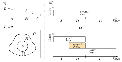
The unitary decomposition technique in Sec.III is generalized from a similar result for short-range interactions in Ref. Haah et al. (2018). We use it to approximate the evolution of a long-range interacting system by three sequential evolutions of its subsystems , , and (see Fig. 1).
We assume that the interaction strength between any two sites in the system is bounded by , with being the distance between the sites and a nonnegative constant.
This restriction on the Hamiltonian norm also sets the time unit for the evolution of the system.
There are two sources of error in the approximation:
one due to the truncation of the Hamiltonian of the system (we ignore the interactions that connect and ),
and the other due to the Hamiltonians of the subsystems , and not commuting with each other.
For a fixed value of , if the distance between the two regions and (see Fig. 1a) is large enough, namely , the two error sources have the same scaling with .
To estimate the error, for example from the truncation, we sum over interactions connecting sites in and , and obtain a total error of (in one dimension) for the approximation in the unitary decomposition (as shown in Sec.A.1).
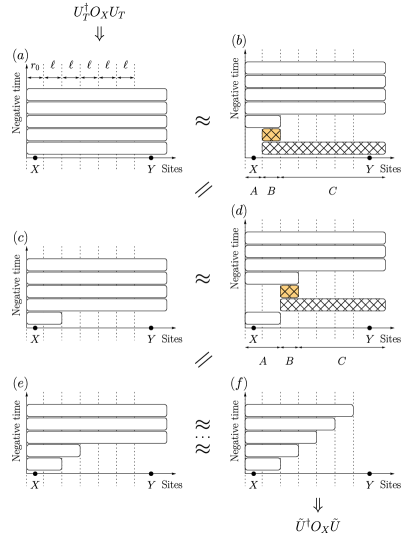
Figure 1: A demonstration of the unitary decomposition in Lemma 1. Panel : the three disjoint regions in and dimensions with convex and compact. Panel : Lemma 1 allows the evolution of the whole system to be approximated by a series of three evolutions of subsystems. The horizontal axis lists the sites in each of the three sets (not necessarily according to their geometrical arrangement, particularly in higher dimensions). Each box is an evolution for time of a Hamiltonian supported on the sites the box covers. These evolutions can be forward (white fill) or backward (orange fill, with dagger) in time.Figure 2: A step-by-step construction of the unitary such that .
Each box represents an evolution of the subsystem covered by the width of the box for a fixed time.
The colors of the boxes follow the same convention as in Fig. 1.
In panel (a), the unitary is written as a product of evolutions of the same system in consecutive time slices. (b) The evolution in the last (bottom) time slice is decomposed using the method in Fig. 1, with the choice of subsystems such that is contained in .
The evolutions of the subsystems and (hatched boxes) therefore commute with and cancel out with their counterparts from , resulting in (c). In panel (d), we repeat the procedure for the second-from-bottom time slice, but note the different choice of from panel (b).
This difference is necessary to ensure that the evolutions of and commute with the evolution(s) from the previously decomposed time slice(s).
We then commute them through again and remove them from the construction of in panel (e).
Repeatedly applying the unitary decomposition for the other time slices, we obtain the unitary in panel (f), which is supported on a smaller region than the original unitary .
With a proper choice of the size of , we can make sure that lies outside this region, and, therefore, commutes with .
In Sec.IV, we use the unitary decomposition to prove a Lieb-Robinson bound for long-range interactions that is stronger than previous bounds, including the one we use in the proof of the unitary decomposition.
The subject of such a bound is usually the norm of the commutator between an operator evolved under a long-range Hamiltonian for time and another operator supported on a set that is at least a distance away from the support of .
Here, we briefly explain the essence of the proof using a one-dimensional system with fixed and large enough as an example.
The strategy is to use the aforementioned unitary decomposition to construct another unitary such that (i) approximates and (ii) commutes with , so the commutator norm will be approximately zero, up to the error of our approximation.
For fixed , we consider equal time slices and use the unitary decomposition to extract the relevant parts from the evolution in each time slice.
Each time we decompose a unitary, we choose the subsystems so that only overlaps with the supports of the unitaries from the previous time slices (see Fig.2), and therefore the evolutions of and can be commuted through to cancel their counterparts from (Fig.2b and Fig.2d):
(1)
The remaining evolutions that contribute to the construction of are supported entirely on a ball of radius around , where is the size of and is chosen to be the same in all time slices.
By choosing and so that lies outside this ball, the commutator norm is at most the number of time slices multiplied by , which is the decomposition error per time slice.
Therefore, we obtain a Lieb-Robinson bound for long-range interactions in one dimension:
(2)
where is a constant that may depend on , but not on .
Setting the commutator norm to a small constant yields the causal region inside the effective light cone: .
For comparison, the previous best Lieb-Robinson bound produces a light cone Foss-Feig et al. (2015).
Our bound is therefore tighter in the asymptotic limit of large and large , while its proof is substantially more intuitive than in Ref. Foss-Feig et al. (2015).
A more careful analysis (Sec.IV) shows that our light cone also becomes linear in the limit , where the power-law decaying interactions are effectively short-range.
Moreover, our bound works for arbitrary time , while the bound in Ref. Foss-Feig et al. (2015) applies only in the long-time limit.
We provide a more rigorous treatment as well as a bound for -dimensional systems in Sec.IV.
SectionV then then discusses the original motivation for the unitary decomposition—digital quantum simulation—in the case of long-range interactions that decay as a power law.
For , our analysis shows that the HHKL algorithm Haah et al. (2018) requires only two-qubit gates to simulate the evolution of a system of sites arranged in a -dimensional lattice for time with an error at most .
For large , the gate count of the algorithm scales with significantly better than other algorithms.
III Framework
In this section, we present the technique for approximating the time evolution of a system by evolutions of subsystems. We later use this technique to derive a stronger Lieb-Robinson bound (Sec.IV) and an improved quantum simulation algorithm (Sec.V) for systems with long-range interactions.
We consider sites arranged in a -dimensional lattice of size and .
Recall that, without loss of generality, we assume the spacing between neighboring lattice sites is one.
This assumption sets the unit for distances between sites in the lattice.
We shall embed the lattice into the real space .
The intersection therefore contains every lattice site in a subset .
The system evolves under a (possibly) time-dependent Hamiltonian
with being the interaction between two sites .
Without ambiguity, we may suppress the time-dependence in the Hamiltonians.
We say a system has power-law decaying interactions if , where denotes both the matrix and the vector 2-norms, for some nonnegative constant and for all . [Note that may have arbitrarily large norm.]
For readability, we denote by the terms of that are supported entirely on a subset , and by the evolution unitary under from time to , where is the time-ordering operator.
We also denote by the minimum distance between any two sites in and , by the complement of in real space, by the boundary of a compact subset , by the area of , and by the union .
In the following, we keep track of how errors scale with time, distance, and , while treating the dimension as a constant.
We now describe how to approximate the evolution of the system to arbitrary precision by a series of evolutions of subsystems using a technique we generalize from Ref. Haah et al. (2018).
Lemma 1.
Let be three distinct regions with non-empty interiors such that . Let be both compact (closed and bounded) and convex.
We have
with
(3)
for all . Here, are positive constants, is a constant that can be chosen arbitrarily in the range , and is the distance between sets and .
We emphasize that this lemma applies to arbitrary sets that are both convex and compact.
The sets we focus on include -balls and hyperrectangles in . The former geometry is relevant in the proof of our new Lieb-Robinson bound, the latter in the analysis of the HHKL algorithm for long-range interactions.
Lemma 1 allows us to approximate the evolution of a long-range interacting system by that of subsystems (Fig. 1).
The features of the function are better understood by considering two limiting cases of physical interest.
First, when is finite and (the distance between and ) is large compared to , the function behaves like
(4)
which decays only polynomially with .
In the second limit, as for a large but finite , we recover from the exponentially decaying error bound —a trademark of finite-range interactions Lieb and Robinson (1972); Haah et al. (2018).
The proof of Lemma 1, while more general, bears close resemblance to the corresponding analysis for short-range interactions in Ref. Haah et al. (2018).
However, there are two key differences.
First, in order to make the approximation in Lemma 1, some interactions between sites separated by a distance greater than are truncated from the Hamiltonian.
While such terms vanish in a system with short-range interactions, here they contribute to the error of the approximation.
In addition, instead of the original Lieb-Robinson bound Lieb and Robinson (1972) which applies only to systems with short-range interactions, we use Gong et al.’s generalization of the bound for long-range interactions Gong et al. (2014).
The result is an approximation error that decays with polynomially as , in addition to the exponentially decaying error that exists already for short-range interactions.
Nevertheless, the error can always be made arbitrarily small by choosing to be large enough.
In Sec.III.1 below, we present the proof of Lemma 1.
After that, we demonstrate the significance of Lemma 1 with two applications: a stronger Lieb-Robinson bound for long-range interacting systems (Sec.IV) and an improved error bound for simulating these systems (Sec.V).
Both sections are self-contained, and readers may elect to focus on either of them.
III.1 Error bound on the unitary decomposition
Here, we will outline the proof of Lemma 1.
Similar to Ref. Haah et al. (2018), we begin with an identity:
(5)
Our aim is to approximate by , from which Lemma 1 will follow.
For that, we look at the generator of Haah et al. (2018), i.e., a Hamiltonian such that
(6)
for all time.
Exact differentiation of yields Osborne (2006); Michalakis (2012)
(7)
(8)
(9)
where denotes the sum of terms supported across disjoint sets and , and are error terms we now define and evaluate.
Note that the first term in Eq. (9) is the generator of —the unitary with which we aim to approximate .
In contrast to the approximation for short-range interacting systems in Ref. Haah et al. (2018), there are two sources of error in Eq. (9).
The first error term arises after we discard from Eq. (7).
For the short-range interactions in Ref. Haah et al. (2018), this error vanishes when the distance between and is larger than the interaction range.
However, in our case, there is a nontrivial truncation error associated with ignoring long-range interactions between and :
(10)
for , where is a constant [Eq.30], is the distance between and .
The factor of in the bound comes from the requirement that the two-body interactions decay as a power law ,
while the term is due to the sum over all sites in the -dimensional set . Another factor of arises after summing over the volume of , which we assume to be a compact and convex set.
The detailed evaluation of the norm is presented in Appendix A.1.
The other error, which we define to be , is the result of the approximation used between Eqs.8 and 9.
In the former equation, the operator evolves under , whereas in the latter, it evolves under the reduced Hamiltonian , thus incurring the error:
(11)
To understand why is small, recall that is the sum of terms that are supported on two sites and .
Since the strengths of such terms decay as (with the distance between the sites and ), the main contribution to —and thus to —comes from the terms where and are spatially close to each other.
But since the sets are separated by a large distance , if the site is close to , then it must be far from . Thus, the evolution of for a short time under can be well-approximated by evolution under alone.
In SectionA.2, we make this intuition rigorous using Gong et al. Gong et al. (2014)’s generalization of the Lieb-Robinson bound to systems with long-range interactions.
In the end, we obtain the following bound on :
(12)
where is a constant [Eq.49] and is a free parameter.
The bound has contributions from two competing terms: one that decays polynomially with and another that decays exponentially.
The polynomially decaying term is dominant for fixed and large , whereas the exponentially decaying term prevails as for fixed .
The errors and in approximating the generator combine to give an overall error in approximating with (see AppendixB). From this, we obtain the error bound in Lemma1, with .
Before discussing applications of Lemma1, we pause here to note that the Lieb-Robinson bound in Gong et al. Gong et al. (2014) used in the above analysis is not the tightest-known bound for long-range interactions Foss-Feig et al. (2015).
Our use of this bound, however, does not lead to a suboptimal error bound in Lemma1. For finite , the error bound is dominated by the polynomially decaying term , which arises from the truncation error rather than . Therefore, this error term would not benefit from a tighter Lieb-Robinson bound.
In the limit , on the other hand, we shall see later that the lemma already reproduces the short-range Lieb-Robinson bound, which is optimal up to a constant factor.
Thus, we expect that using stronger Lieb-Robinson bounds would produce no significant improvement for the error bound in Lemma1.
IV A stronger Lieb-Robinson bound
In this section, we will use Lemma 1 to derive a stronger Lieb-Robinson bound for long-range interactions.
The first generalization of the Lieb-Robinson bound to power-law decaying interactions was given by Hastings and Koma Hastings and Koma (2006).
However, their bound diverges in the limit , where the power-law decaying interactions are effectively short-range.
Later, Gong et al. Gong et al. (2014) derived a different bound that, in this limit, does indeed converge to the Lieb-Robinson bound for short-range interactions.
While we used this bound in Sec.III to prove Lemma 1, we will also show that by using this lemma, we can in turn derive a Lieb-Robinson bound for long-range interactions that is stronger than the one in Gong et al. In fact, our bound produces a tighter effective light cone than even the strongest Lieb-Robinson bound for long-range interactions known previously Foss-Feig et al. (2015).
Recall that the subject of a Lieb-Robinson bound is the commutator norm
(13)
where are two operators supported respectively on two sets geometrically separated by a distance , and is the time-evolution unitary of the full lattice under a power-law decaying Hamiltonian, as defined above.
To compare different bounds, we analyze their effective light cones, which, up to constant prefactors, predict the minimum time it takes for the correlator to reach a certain value.
For example, the original Lieb-Robinson bound Lieb and Robinson (1972) produces a linear light cone
for short-range interactions.
For long-range interactions, Hastings and Koma Hastings and Koma (2006) first showed that for some (-dependent) constants .
By setting equal to a constant, the bound gives an effective light cone
in the limit of large and .
Gong et al. Gong et al. (2014) later achieved a tighter light cone that is linear for short distances and becomes logarithmic only for large .
Shortly after, Foss-Feig et al. Foss-Feig et al. (2015) derived a bound with a polynomial light cone:
(14)
Equation14 was the tightest light cone known previously.
In the remainder of this section, we use Lemma 1 to derive a Lieb-Robinson bound for long-range interactions that produces an effective light cone tighter than the one in Ref. Foss-Feig et al. (2015), while also using a much more intuitive approach.
In addition, our bound works for all times, unlike the bound in Ref. Foss-Feig et al. (2015), which applies only in the long-time limit.
Theorem 1(Lieb-Robinson bound for long-range interactions).
Suppose is supported on a fixed subset .
For , we have
(15)
Here is the distance between the supports of and , are constants that may depend only on [defined in AppendixC], and is given by Eq.3.
Before we prove Theorem1, let us analyze the features of the bound.
Although the general bound in Eq.15 looks complicated, it can be greatly simplified in some limits of interest.
For example, for finite , in the limit of large and large such that , the term algebraically decaying with in dominates the exponentially decaying one [see also Eq.3 and Eq.72].
Therefore, the Lieb-Robinson bound in this limit takes the form:
(16)
where is finite and may depend on [Eq.74].
We can immediately deduce the effective light cone given by our bound for a finite :
(17)
which is tighter than Eq.14 (as given by Ref. Foss-Feig et al. (2015)).
In particular, for close to , the exponent in Eq.17 can be almost twice that of Ref. Foss-Feig et al. (2015) (the larger the exponent, the tighter the light cone).
On the other hand, in the limit , is finite and therefore always less than .
Hence our bound converges to the short-range bound .
We note that in this limit, the exponent of the light cone in Eq.17 also converges to one, which corresponds to a linear light cone, at a linear convergence rate [see Eq.76 for details].
These behaviors are naturally expected since a power-law decaying interaction with very large is essentially a short-range interaction.
As mentioned earlier, we derive Theorem1 by constructing a unitary such that (i) approximates and (ii) commutes with .
We note that does not necessarily approximate .
It then follows from the two requirements that the commutator norm , defined in Eq.13, is upper bounded by the error of the approximation in (i).
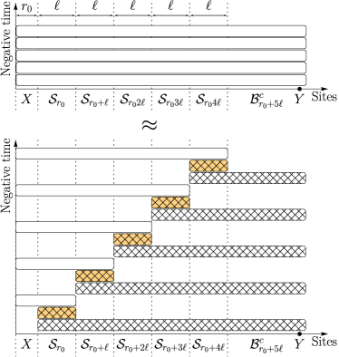
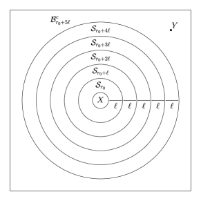
Figure 3: A construction of the unitary which results in an improved Lieb-Robinson bound for long-range interactions in Theorem 1.
The horizontal axes list the sites in each subset.
Here denotes a -ball of radius centered on , and a -dimensional shell of inner radius and outer radius , for some parameter to be chosen later. (See Fig.7 in AppendixC for an illustration of the sets.)
The evolution unitaries are represented by boxes with the same color convention as in Fig. 1.
We first divide the interval into equal time slices (upper panel).
Note that because we consider in the Heisenberg picture, the vertical axis is therefore backward in time so that the bottom time slice will correspond to the first unitary applied on .
The evolution during each time slice is approximated by three evolutions of subsystems using Lemma 1 (lower panel).
The bottom two unitaries have their supports outside and therefore commute with .
They cancel with their Hermitian conjugates from in .
Repeating the argument for higher time slices, we can eliminate some unitaries (hatched boxes) from the construction of .
Finally, we are left with consisting only of unitaries (white boxes) that are supported entirely on the -ball of radius .
Therefore, commutes with , whose support lies in the complement of .
We also note that the assumption on the norms of the interactions being bounded excludes several physical systems whose local dimensions are unbounded, e.g. bosons [see Ref. Eisert and Gross (2009); Jünemann et al. (2013) for discussions of information propagation and Lieb-Robinson bounds in these systems].
However, our Lieb-Robinson bound may still apply if the dynamics of the systems can be restricted to local Hilbert subspaces which are finite-dimensional.
Examples of such situations include trapped ions in the perturbative regime Kim et al. (2011) and noninteracting bosons Deshpande et al. (2018).
To construct , we use Lemma1 to decompose the unitary into unitaries supported on subsystems, each of which either contains or is disjoint from .
The unitaries of the latter type can be commuted through to cancel out with their Hermitian conjugates from .
The remaining unitaries form , which is supported on a smaller subset than .
In particular, with a suitable decomposition, the support of can be made to not contain , and, therefore, commutes with .
The step-by-step construction of the unitary has also been briefly described earlier in Sec.II and in Fig.2, using the specific case of a one-dimensional system with a finite .
This construction immediately generalizes to higher dimensions and to arbitrary , including the limit.
The construction of for arbitrary is summarized in Fig.3.
We note that there is more than one way to decompose the unitary in the construction of .
Different constructions of result in different approximation errors, each of which provides a valid bound on the commutator norm .
Therefore, the goal is to find a construction of with the least approximation error.
In AppendixC, we present the construction that results in the bound in Theorem1.
Although we have evidence suggesting that the construction is optimal, we do not rule out the existence of a better construction.
V Better performance of digital simulation
In this section, we generalize the algorithm in Ref. Haah et al. (2018) to simulating long-range interactions.
In general, the aim of quantum simulation algorithms is to approximate the time evolution unitary using the fewest number of primitive, e.g. two-qubit, quantum gates.
Here, we show that in addition to the stronger Lieb-Robinson bound presented in the previous section, Lemma 1 can also be used to perform error analysis for the HHKL algorithm (Ref. Haah et al. (2018)) in the case of interactions that decay as a power law,
therefore improving the theoretical gate count of digital quantum simulation for such interactions.
Using the best known rigorous error bounds, simulations based on the first-order Suzuki-Trotter product formula Lloyd (1996) use gates to simulate the evolution of a time-dependent Hamiltonian on sites up to a fixed error .
(In this section, the big is with respect to and .)
The generalized ()th-order product formula uses quantum gates.
While this scaling asymptotically approaches as , it suffers from an exponential prefactor of Berry et al. (2007).
More advanced algorithms, e.g., those using quantum signal processing (QSP) Low and Chuang (2017) or linear combinations of unitaries (LCU) Berry et al. (2015), can reduce the gate complexity to .
Our error analysis below (Lemma2) reveals that, when is large, the number of quantum gates required by the HHKL algorithm to simulate long-range interactions scales better as a function of the system size than previous algorithms.
The HHKL algorithm itself uses either the QSP algorithm or the LCU algorithm as a subroutine to simulate the dynamics of a subset of the sites for one time step. Although the QSP algorithm does not handle time-dependent Hamiltonians, LCU can be applied to time-dependent Hamiltonians.
Our results assume that (i) the local terms have bounded norms for all , and (ii) the Hamiltonian varies slowly and smoothly with time so that exists and scales at most polynomially with for all subsets .
These restrictions allow portions of the system to be faithfully simulated using LCU (or QSP, for a time-independent Hamiltonian).
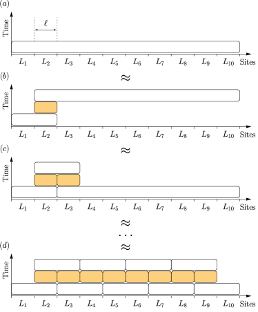
Figure 4: A demonstration of the HHKL decomposition Haah et al. (2018) of the evolution of a fixed time interval for a system with blocks, each consisting of sites.
As before, each box represents a unitary (white) or its Hermitian conjugate (orange) supported on the covered sites.
Using Lemma 1, the HHKL decomposition approximates the evolution of the whole system [panel (a)] by three unitaries supported on subsystems [panel (b)].
By applying Lemma 1 repeatedly [panels (c) and (d)], the evolution of the whole system is decomposed into a series of evolutions of subsystems, each of size at most .
V.1 HHKL-type algorithm for simulating long-range interactions
Although Ref. Haah et al. (2018) focused on simulating short-range interactions, their (HHKL) algorithm can also be used to simulate long-range interactions.
Here, we analyze the performance of their algorithm in simulating such systems.
In the HHKL algorithm Haah et al. (2018), the evolution of the whole system is decomposed, using Lemma 1, into elementary unitaries, each evolving a subsystem of at most sites, where is again a length scale to be chosen later.
For a fixed time , the algorithm simply simulates each of these elementary unitaries using one of the existing quantum simulation algorithms.
In particular, we shall use LCU or (for a time-independent Hamiltonian) QSP due to their logarithmic dependence on the accuracy.
In this section, we assume is finite and analyze the gate count in the limit of large system size .
As a consequence, the block size can also be taken to be much larger than .
For simplicity, we will not keep track of constants that may depend on .
Recall that in this limit, the error bound in Lemma1 is at most
(18)
where we have assumed .
Using Lemma1, we obtain the error bound for the first step of the HHKL algorithm, which can be summarized by the following lemma.
Lemma 2(HHKL decomposition).
There exists a circuit that approximates up to error , where is a free parameter. The circuit has depth at most and consists of elementary unitaries, each of which evolves a subsystem supported on at most sites for time .
Proof.
We now demonstrate the proof by constructing the circuit for a one-dimensional lattice (Fig. 4). A generalization of the proof to arbitrary dimension follows the same lines and is presented in AppendixD.
First, we consider equal time intervals such that is a constant for all .
The simulation of then naturally decomposes into consecutive simulations of .
We then divide the system into consecutive disjoint blocks, each of size (Fig. 4).
Denote by the set of sites in the -th block.
Using Lemma 1, we can approximate
(19)
This approximation can be visualized using the top two panels of Fig. 4.
Repeated application of Lemma 1 yields the desired circuit (bottom panel of Fig. 4), with each elementary unitary evolving at most sites for time .
To obtain the error estimate in Lemma 2, we count the number of times Lemma 1 is used in our approximation.
In each of the time slices, we use the lemma times, each of which contributes an error of [see Eq.18 with in one dimension].
Therefore, with , the error of using the constructed circuit to simulate is
The error bound for the approximation in Lemma2 leads to an upper bound on the gate complexity of digital quantum simulation, as stated in the following theorem.
Theorem 2.
For , there exists a quantum algorithm for simulating up to error at most with gate complexity
(21)
This gate complexity can be achieved by applying the HHKL algorithm Haah et al. (2018) for long-range interactions, as described above.
First, the evolution of the whole system is approximated by elementary unitaries as provided in Lemma 2.
Each of these elementary unitaries is then simulated using one of the existing algorithms, e.g., LCU, with error that we require to be at most .
If the Hamiltonian is time-independent, one can also use the QSP algorithm to simulate the elementary unitaries.
In the decomposition of the evolution, the accuracy of the approximation can be improved by increasing the block size .
By Lemma 2, to achieve an overall error at most , we need
(22)
When simulating the elementary unitaries, since each is an evolution of at most sites for time , the LCU algorithm with error at most uses two-qubit gates Berry et al. (2007).
Recall that we assume scales at most polynomially with .
With the block size from Eq. (22), we find the total gate complexity of simulating the elementary unitaries is
(23)
(24)
The scaling of as a function of the system size is significantly better than existing algorithms for large . In particular, at , this HHKL algorithm for long-range interactions requires only gates, while algorithms such as QSP or LCU use gates or more.
Therefore, the algorithm provides an improvement for .
However, the gate complexity of the algorithm depends polynomially on , in contrast to the logarithmic dependence achieved by QSP and LCU, and by the HHKL algorithm for systems with short-range interactions.
While this scaling is undesirable, in practice, the total error of the simulation is often set to a fixed constant (for example, see Ref. Babbush et al. (2015)) and effectively the dependence of only contributes a prefactor to the gate complexity of the algorithm.
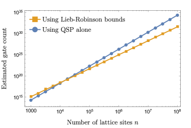
As an example, in Fig.5, we estimate the actual gate count of the HHKL algorithm in simulating a Heisenberg chain [Eq.25] and compare it with the gate count of the QSP algorithm (up to the same error tolerance).
Because of the overhead, the HHKL algorithm based on Lieb-Robinson bounds uses more quantum gates for simulating small systems, but eventually outperforms the QSP algorithm when the system size is large.
Figure 5: The gate count for simulating the dynamics of a one-dimensional Heisenberg chain [Eq.25] of length , with and .
We compare the gate count of the HHKL algorithm (orange square) to the QSP algorithm (blue circle).
Note that the HHKL algorithm based on Lieb-Robinson bounds also uses the QSP algorithm as a subroutine.
We obtain the scatter points using the approach described in AppendixE and fit them to a power-law model (solid lines).
The asymptotic scalings of the gate count obtained from the power-law fits ( for HHKL, for QSP) agree well with our theoretical predictions (see Table1).
It is also worth noting that, in the limit , the gate complexity becomes , which coincides (up to a polylogarithmic factor) with the result for short-range interactions in Ref. Haah et al. (2018).
This behavior is expected, given that a power-law decaying interaction with is essentially a nearest-neighbor interaction.
However, we caution readers that at the beginning of this section, we have assumed that is finite so that . Hence, the gate count in Eq.24 is technically not valid in the limit .
Nevertheless, the error bound in Lemma1 reproduces the estimate for short-range interactions in Ref. Haah et al. (2018), and therefore, repeating the argument of this section in the limit should also reproduce the gate count for simulating short-range interactions in Ref. Haah et al. (2018).
V.2 Numerical evidence of potential improvement
Up to now, we have seen that Lieb-Robinson bounds can improve the error bounds of quantum simulation algorithms, as demonstrated by the HHKL algorithm.
We now provide numerical evidence hinting at the possibility of further improving the error bounds.
Although the HHKL algorithm outperforms previous ones when , it remains an open question whether there is a faster algorithm for simulating long-range interactions.
We also note that the gate complexities are only theoretical upper bounds, and these algorithms may actually perform better in practice Childs et al. (2017).
As an example, we compute the empirical gate count of a Suzuki-Trotter product formula simulation of a one-dimensional long-range interacting Heisenberg model
(25)
where are chosen uniformly at random and denotes the vector of Pauli matrices on the qubit .
Specifically, we consider a simulation using the fourth-order product formula (PF4).
We use a classical simulation to determine the algorithm’s performance for systems of size to for time , and extrapolate to larger systems.
For each , we search for the minimum number of gates for which the simulation error is at most .
We plot in AppendixF this empirical gate count, which appears to
scale only as with the system size .
We list in Table1 the gate counts of several popular algorithms for comparison.
The theoretical gate complexity of PF4 is Lloyd (1996), while the QSP and LCU algorithms both have complexity .
These numerics show that the PF4 algorithm for simulating long-range interacting systems performs better in practice than theoretically estimated; in fact, it even performs almost as well as the HHKL algorithm based on Lieb-Robinson bounds [which scales as by our earlier analysis].
Whether other quantum simulation algorithms, including the HHKL algorithm, can perform better than suggested by the existing bounds remains an important open question.
Table 1: A comparison between the gate complexity of several quantum simulation algorithms for simulating one-dimensional power-law systems at and .
Our analysis shows that the HHKL algorithm performs at least as well as the empirical gate count of PF4, while having a similar scaling with the error .
It is not known whether the empirical gate count of PF4 can scale with better than suggested by the best proven bound (the third row).
VI Conclusion & outlook
To conclude, we derived an improved bound on how quickly quantum information propagates in systems evolving under long-range interactions.
The bound applies to power-law interactions with , such as dipole-dipole interactions in 1D (often realizable with nitrogen-vacancy centers Maze et al. (2011) or polar molecules Yan et al. (2013)), trapped ions in 1D Britton et al. (2012); Kim et al. (2011), and van-der-Waals-type interactions between Rydberg atoms Saffman et al. (2010) in either 1D or 2D.
For finite , our Lieb-Robinson bound gives a tighter light cone than previously known bounds—including the one used in the proof of Lemma 1.
As of yet, we are not aware of any physical systems that saturate the Lieb-Robinson bounds for power-law interactions, including the new bound.
In the limit , our bound asymptotically approaches the exponentially decaying bound for short-range interactions.
Our bound gives a linear light cone only in this limit, however, and it remains an open question whether there exists a stronger bound with a critical such that the light cone is exactly linear for Luitz and Bar Lev (2019).
Currently, there are no known methods for quantum information transfer that are faster than linear for .
It is possible, therefore, that a stronger bound exists with a finite .
It is our hope that the present work, as well as the techniques that we use, will help motivate the search for such stronger bounds.
Our technique immediately extends the HHKL algorithm in Ref. Haah et al. (2018) to the digital quantum simulation of the above systems.
Our error bounds indicate that the gate complexity of the algorithm is better than that of other state-of-the-art simulation algorithms when is sufficiently large (), and matches that of the short-range algorithm when .
However, the empirical scaling of other algorithms—such as product formulas—indicates that this gate complexity may only be a loose upper bound to the true quantum complexity of the problem.
While a matching lower bound for the gate complexity of the HHKL algorithm is provided in Ref. Haah et al. (2018) for Hamiltonians with short-range interactions, we do not know of any techniques that could provide a corresponding bound for long-range interactions.
In addition to improving the quantum gate complexity, our results may also aid in the design of better classical algorithms for simulating long-range interacting quantum systems.
In particular, while we still expect the classical gate complexity to be exponential in the simulation time, there may be room for a polynomial improvement.
While the use of Lieb-Robinson bounds to improve the performance of quantum algorithms is a natural extension of Haah et al., the opposite direction—using quantum algorithms to improve Lieb-Robinson bounds—is new.
The connection from quantum simulation algorithms to Lieb-Robinson bounds that we have established opens another avenue for the condensed matter and atomic/molecular/optical physics communities to potentially benefit from future advances in quantum algorithms.
In addition to proving a stronger Lieb-Robinson bound, the tools we developed may help to answer other questions regarding both short-range and long-range interacting systems.
Using the same unitary construction as Theorem1, we can generalize the bounds on connected correlators Bravyi et al. (2006b); Tran et al. (2017) to long-range interacting systems.
Our results can also provide a framework for proving tighter bounds on higher-order commutators, such as out-of-time-order correlators Larkin and Ovchinnikov (1969); Kitaev and Suh (2018).
Previous methods used to derive Lieb-Robinson bounds—due to their use of the triangle inequality early in their proofs—have not been able to capture the nuances in the growth of such correlators.
In addition to the more intuitive proof of the Lieb-Robinson bounds, our framework can be used to provide an alternative, simpler proof of the classical complexity of the boson-sampling problem Aaronson and Arkhipov (2011), which generalizes the result in Ref. Deshpande et al. (2018) to long-range interactions and also to more general Hamiltonians with arbitrary local interactions Bos .
By taking advantage of the unitary decomposition in Lemma1, we obtain a longer time interval within which the sampler in Ref. Deshpande et al. (2018) is efficient Bos .
Moreover, by generalizing from two-body to many-body interactions, our technique may find applications in systems whose Hamiltonians include interaction terms between three or more sites, e.g. many-body localized systems in the -bit basis Serbyn et al. (2014).
Note added:
Shortly after we submitted our paper to arXiv, Else et al. Else et al. posted their work on a different Lieb-Robinson bound for power-law decaying interactions.
For Hamiltonians consisting of at most two-body interactions, the bound in Ref. Else et al. and our bound both apply in the same regime, 111
Note that there is a difference between the definition of the exponent in Ref. Else et al. and in this paper.
For two-body Hamiltonians, the exponent in Ref. Else et al. is equal to our minus the dimension .
Within this regime, our bound results in a strictly tighter light cone than Ref. Else et al..
However, the bound in Ref. Else et al. also applies to Hamiltonians consisting of -body interactions, for any integer .
Generalizing our framework to cover such -body interactions would be an interesting future direction.
Acknowledgements.
We thank G. H. Low, A. Deshpande, P. Titum, T. Zhou, and Z.-X. Gong for helpful discussions.
MCT, AYG, ZE and AVG acknowledge funding from the U.S. Department of Energy ASCR Quantum Testbed Pathfinder program (Award No. DE-SC0019040), ARO MURI, ARO, NSF Ideas Lab on Quantum Computing, ARL CDQI, NSF PFC at JQI, AFOSR, and the U.S. Department of Energy BES Materials and Chemical Sciences Research for Quantum Information Science program (Award No. DE-SC0019449).
AMC and YS acknowledge funding from ARO MURI, CIFAR, NSF, and the U.S. Department of Energy, Office of Science, Office of Advanced Scientific Computing Research, Quantum Algorithms Teams and Quantum Testbed Pathfinder programs (Award No. DE-SC0019040).
MCT is supported in part by the NSF Grant No. NSF PHY-1748958 and the Heising-Simons Foundation.
AYG is supported by the NSF Graduate Research Fellowship Program under Grant No. DGE 1322106.
JRG is supported by the NIST NRC Research Postdoctoral Associateship Award and performed his work in part at the Aspen Center for Physics, which is supported by National Science Foundation grant PHY-1607611.
ZE is supported in part by the ARCS Foundation.
In this subsection, we provide explicit calculations of in Eq. (10).
Recall that is the shortest distance between any two points in and .
Therefore, is always greater than .
For each , let be the minimum distance from to the set and .
Clearly, is a subset of .
Therefore,
(26)
(27)
(28)
where is a constant independent of and the sum over is bounded using Lemma 5 in AppendixG.
Next, to evaluate the sum over , we parameterize the sites in the set by their distance to its boundary .
Note that by assumption the interior of is non-empty, so that .
Roughly speaking, there will be at most sites whose distances to the boundary is between and , for each , where is the boundary area of .
Therefore, we have (see Lemma9 in SectionG.2 for a rigorous proof)
(29)
(30)
for ,
where is a constant that arises after using Lemma5 to bound the sum, and the factor is because we lower bound to simplify the expression.
The constants are later absorbed into the definition of .
A.2 Evaluation of
In this section, we show how we bound from Eq.11 in the proof of Lemma1.
To estimate , we use the following lemma, which generalizes a similar lemma in Ref. Haah et al. (2018) to arbitrary, time-dependent Hamiltonians.
Lemma 3.
Let be a subset of sites.
Let be the terms of supported entirely on .
Let be an observable supported on a subset at a fixed time .
We have:
(31)
where .
Proof.
To prove the lemma, we shall move into the interaction picture of and treat as a perturbation.
Let and be respectively the Hamiltonian and the evolution operator in the interaction picture.
We have:
By substituting , , , and noting that operators supported on disjoint subsets commute, we can show using Lemma 3 that
(36)
where the observables are, in general, evaluated at different times .
We note that while it is necessary to keep track of for completeness, one should pay more attention to the supports of the operators, as they carry useful information about the locality of the system.
In fact, let us pause for a moment to discuss why the right hand side of Eq. (36) should be small when , the distance between and , is large.
Whenever the supports of and are far from each other, we can bound their commutator norm using a Lieb-Robinson bound for long-range interactions.
We use the bound by Gong et al. Gong et al. (2014):
(37)
where is the distance between the supports, is a constant that can be made arbitrarily close to 1, and are constants that depend only on .
Figure 6: An illustration of and in a one-dimensional lattice.
For short-range interactions, the sets and are separated by a distance of the same order as the size of (upper figure).
The contributions from these terms to are bounded using a Lieb-Robinson bound.
However, for long-range interactions, and can be geometrically close to each other (lower figure).
In such cases, the norms of and decay as and and, therefore, their contributions to are small.
However, in contrast to short-range interacting systems, here run over all possible sites in , so in principle the distance between the supports of and can be small (Fig. 6).
Fortunately, if that is indeed the case, then although the Lieb-Robinson bound is trivial, the assumption that and fall off as and , respectively, makes the summand in Eq. (36) small.
Let us now evaluate the sum in Eq.36.
In the following, we shall consider , since the estimation for the case follows a similar, but less complicated argument.
Using Gong et al.’s Lieb-Robinson bound for long-range interactions Gong et al. (2014):
(38)
where is a constant that can be chosen arbitrarily close to 1, while are finite and bounded constants for all , and
(39)
is the distance between the supports of and (see Fig.6).
Since each term of contributes a sum of an algebraically decaying as and an exponential decaying as terms, it is convenient to evaluate their contributions separately.
First, let us find the contribution from the algebraically decaying part.
It is straightforward to find out their contributions to when takes one of the four allowed values.
Depending on which value takes, we use either Lemma 5 or Lemma 7 in AppendixG to evaluate the sums over and .
For example, the contribution from the terms where is at most
(40)
(41)
(42)
where are constants that arise after we use Lemma 7 in AppendixG twice to evaluate the sums over and consecutively, and the sums over have been bounded in the previous section (see Eq.27).
The constant absorbs both and the constants from the sums over .
On the other hand, if , we use Lemma 7 to evaluate the sum over and Lemma 5 for the sum over :
(43)
(44)
(45)
where come from the uses of Lemma7 and Lemma5 respectively.
The constant absorbs both and the constants from the sums over .
Repeating for the other values of , we find that the contribution from the algebraically decaying terms in Equation38 to is at most
(46)
for some constant .
Next, let us find the contribution from the exponentially decaying term in Equation38.
If , we have
(47)
where we have applied Lemma8 in AppendixG to obtain the first inequality, Lemma8 twice again and Lemma7 to get the second inequality, and then Lemma5 and Lemma6 for the sums over similarly to SectionA.1.
The constants arise from the applications of the lemmas and are absorbed into a constant .
We note that the constant in the last three lines are different from the one in the first line (see Lemma8 for details).
However, they both are constants that can be chosen arbitrarily between 0 and 1. Therefore, we denote them by the same constant for convenience.
Repeating the argument for other choices of in Eq.39, we find that the contribution from the exponentially decaying terms to is still at most the right hand side of Eq.47.
for a constant .
Since for any arbitrary small positive constant , we can upper bound
(49)
where we have absorbed into the definition of and .
This completes the estimation of .
Appendix B Error propagation from generating function
In this section, we reproduce a lemma in Ref. Haah et al. (2018) which shows how the error in approximating the generating function propagates to an error of the unitary in Eq.6.
Suppose we approximate by such that
(50)
for some function of time and is time-independent.
We shall prove that the unitary generated by approximates with error
(51)
Proof.
By simple differentiation, we have
(52)
(53)
(54)
(55)
(56)
∎
Appendix C Proof of the Lieb-Robinson bound for long-range interactions
We present a more detailed proof of Theorem1 in this section.
The key ingredient in the proof of Theorem 1 is the following lemma.
Lemma 4.
Denote by a -ball of radius centered around the origin.
Let be an observable supported on with being finite.
For each and a positive integer , there exists a unitary supported on a -ball with such that
(57)
where is a constant, and is a free parameter.
Proof.
Figure 7: An example of the subset and five shells for . The operator is supported on , which lies on , the complement of the ball .
We shall prove the lemma by constructing the unitary .
In addition to above, we define
(58)
to be a shell consisting of sites between and away from the origin (Fig.7).
We divide into equal time intervals, namely for , where .
The unitary then naturally decomposes into a product of unitaries :
(59)
We now use Lemma 1 to further decompose each into evolutions of subsystems.
We start with and use Lemma 1 with , and (Fig. 3) to decompose (instead of ):
(60)
where again denotes the complement subset , and is the boundary area of .
This choice of decomposition allows us to eliminate the contribution to the evolution from the terms of the Hamiltonian that commute with , i.e. those supported entirely on .
Explicitly, we have:
(61)
(62)
where is supported entirely on .
If we repeat the above argument for but with replaced by , we can approximate
(63)
for some supported entirely on .
The error of this approximation is at most
By induction to all , we can construct such that
(64)
where the overall error is at most
(65)
(66)
and where we have replaced the surface area of a -ball by and by .
Also by induction, the unitary is supported entirely on .
Therefore the lemma follows.
∎
We are now ready to prove our Lieb-Robinson bound in Theorem 1.
Without loss of generality, we assume the origin is in .
Since , there exists such that is a subset of .
By Lemma4, there exists a unitary supported entirely on a -ball with such that
(67)
If we choose the number of time slices () and the block size () such that , the set will lie outside the support of , and therefore will commute with .
Note that for a fixed value of , the error should decrease with a larger value of .
Therefore, to prove the strongest bound, we should choose as large as possible, i.e., , and hence .
Substituting the value of and into Eq.67, we obtain the error bound in terms of alone:
(68)
where is a finite constant.
We note that the above bound is valid for all values of .
The tightest bound can therefore be obtained by choosing a value for that minimizes the above expression.
Our intuition and numerical evidence suggest that this happens when , so in the below analysis, we aim to choose as close to this value as possible.
To proceed, we consider two regimes of time , when and when .
In the former regime, we choose and substitute into Eq.68 to get
(69)
where we have used for all , and .
In particular, if , where is the larger solution of , the algebraically decaying term in dominates the exponentially decaying one, and therefore
(70)
(71)
(72)
Combining Eqs.69 and 72, we obtain a bound on the commutator norm:
(73)
where
(74)
The light cone implied by the bound is
(75)
In the limit , the exponent of the light cone converges to one at a rate given by
(76)
On the other hand, if , we simply choose .
Equation68 then becomes
(77)
Therefore, we arrive at the Lieb-Robinson bound in Theorem1 with .
In this section, we discuss the construction of the circuit in Lemma 2 that generalizes the lemma to higher dimensions.
Similar to the case, we first break the unitary into unitaries for some .
We then use an algorithm consisting of steps to break the simulation of into simulations of Hamiltonians on smaller hypercubes of size at most .
In the first of the steps, we cut the -dimensional lattice into layers, each with the same thickness , a parameter to be chosen later.
In this step, the cross section of the cut is .
Therefore, by Lemma1, each time a new layer is generated, we accumulate an error of
For layers of the first step, the accumulated error will be .
Next, for each of the layers of dimensions, we break them again into layers of dimensions. Using Lemma 1 with a cross section , we find the error of the second step
(78)
which decreases with faster than the error of the first step.
More explicitly, in the th of the steps, the error is , which is dominated by the error in the first step for all .
Therefore, the error of cutting the -dimensional lattice of size into subsystems is still .
To meet a fixed total error , we need to choose .
The geometrical constraint requires .
Finally, simulating each of the subsystems using the LCU algorithm up to accuracy requires quantum gates.
Therefore, the overall gate complexity of the algorithm is
(79)
Appendix E Estimation of the actual gate count
In this section, we describe how we estimate the actual gate count of the HHKL algorithm and the QSP algorithm in simulating one-dimensional power-law systems.
The direct implementation of the QSP algorithm requires computing a sequence of rotation angles on a classical computer, which is prohibitive for large-size Hamiltonian simulation. Instead, we use a suboptimal approach described in Ref. Childs et al. (2017). To simulate for time and accuracy , where is the number of terms in the Hamiltonian, and are both unitary and Hermitian, we divide the entire evolution into segments. We choose sufficiently large so that each segment is short enough for the classical preprocessing. Specifically, we choose
(80)
and Haah . Within each segment, we choose to be the smallest positive integer satisfying
(81)
so that the overall error is at most . This gives phased iterates within each segment Childs et al. (2017).
The number of elementary operations of each phased iterate is . Here, the first term corresponds to the reflection along an -dimensional state ; the second term costs the preparation/unpreparation of an -dimensional state; and the third term is the cost of selecting two-body operators. We thus estimate the gate complexity of the QSP algorithm as .
Next, in order to determine the gate count of the HHKL algorithm, we need an estimate for the error of the unitary decomposition in Lemma1.
Recall that for , the error given by our analysis is , where is a constant that can be estimated numerically by computing the actual error for small values of and extrapolating for larger .
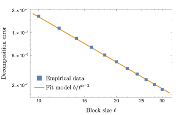
Figure 8:
The empirical error of the unitary decomposition in Lemma1, computed for the single-excitation one-dimensional Heisenberg chain () in Eq.25 at different values of .
The system size is fixed at and the evolution time at .
We fit the data (blue square) to the theoretical model and obtain .
Since simulating the evolution of a generic system is classically intractable even for a moderate system size, we study only the one-dimensional Heisenberg model given in Eq.25 and restrict our calculation to the single-excitation subspace.
In Fig.8, we plot the error of the unitary decomposition in Lemma1 at several different values of (for system size and evolution time ).
The scaling of the error agrees well with our prediction.
By fitting the data to , we obtain an estimate .
Recall that there are time slices in the HHKL algorithm.
In each time slice, there are blocks of size and blocks of size .
To meet the total error at most , we need to choose (see also Eq.20)
(82)
By multiplying the number of blocks by the gate count for using QSP to simulate a single block, we arrive at the total gate count presented in Fig.5.
Appendix F Numerical performance of the product formula
This section includes the numerical performance of the fourth-order product formula (PF4) used to simulate the evolution of the system given in Eq.25 for time .
We plot this numerical performance as well as the theoretical estimates for the gate counts of the PF4, LCU, QSP, and HHKL algorithms in Fig.9.
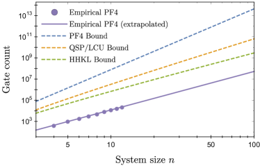
Figure 9:
The empirical gate count of PF4 (purple dots) from to , extrapolated to larger system sizes (solid, purple), for simulating the dynamics of the Hamiltonian in Eq. (25) for time at a fixed error tolerance.
The error bars are smaller than the size of the markers and hence not visible in the plot.
Also shown in dashed lines are the slopes of the gate counts of several advanced algorithms for comparison.
These slopes represent the scaling of the gate counts as functions of . Their -intercepts, which represent a constant multiplicative factor, should be ignored.
Appendix G Mathematical tools
This section contains a collection of mathematical results omitted from the previous sections.
In SectionG.1, we present the upper bounds on standard sums we use in the proof of Lemma1 in AppendixA.
In SectionG.2, we show how we estimate the sum over the convex set in Eq.28 by parameterizing the elements of the set by their distance to the boundary of .
We also note that we use the same notation “” for constants that appear in different lemmas.
Let be a -dimensional lattice and be the coordinates of sites in .
For and , there exists a constant that may depend on but not on such that:
(83)
In particular, it implies that the sum converges for all .
Proof.
The proof of this bound is straightforward.
For simplicity, we first assume none of the coordinates of is zero.
Since is a decreasing function of for all , we can always bound the sum over such by an integral
(84)
where denotes the sum over with no zero coordinate and .
Next, consider with exactly one zero coordinate.
These sites lie on hyperplanes, each of dimension . Therefore the contribution from them can be evaluated using the above integral with :
(85)
By repeating this argument for the sums over with different number of zero coordinates, we arrive at
(86)
where is a constant independent of .
∎
Lemma 6.
Let be a -dimensional lattice and be the coordinates of sites in .
For all , there exists a constant that may depend on but not on such that:
(87)
where is a positive constant.
In particular, it also implies that the sum converges.
Proof.
The proof of this lemma follows the same idea as of Lemma5.
However, note that the function is a decreasing function of only when for some that depends only on .
Therefore, if , we follow the exact same lines as in the proof of Lemma5.
For example, if none of the coordinates of is zero, we can bound
(88)
(89)
for some constants that depend only on .
On the other hand, if , we consider
(90)
The lemma should follow if we can argue that can be chosen independently of .
Indeed, since and from the previous calculation, we know that the sum over converges to a constant that depends only on .
This concludes the proof of Lemma6.
∎
Lemma 7.
Let be three distinct sites in a -dimensional lattice .
For all ,
(91)
where is a constant independent of .
Proof.
A proof of the lemma is presented in Ref. Hastings and Koma (2006).
∎
Lemma 8.
Let be three distinct sites in a -dimensional lattice .
For all , , and positive integers , there exists a constant such that
(92)
where are constants that may depend on , but not on .
Proof.
Without loss of generality, assume .
Let be the distance between and .
We need to prove
(93)
Let be a -ball of radius centered around for some arbitrary constant .
We shall divide the sum over into two regimes, corresponding to
inside and outside .
In the first regime where is inside , we can show using the triangle inequality that . Therefore, the sum over these can be bounded by
(94)
where we have used the fact that converges and is bounded by a constant which may depend only on .
In the second regime, we bound to obtain
(95)
where the last sum is bounded using Lemma6 and noting that .
Let and take , it is straightforward to show that , and therefore,
(97)
Note that if we choose , then takes on a value between 0 and 1, which can be arbitrarily close to 1.
∎
G.2 Parameterizing a convex set
In this subsection, we show how we evaluate the sum over in Eq.28.
First, we parameterize a convex set by the distance to its boundary.
The following lemma simplifies a sum over every site in a convex set to a sum over the above distance, multiplied by the boundary area of the set.
Lemma 9.
Let be a compact and convex set in with non-empty interior. Let be another subset disjoint from ,
and let be the smallest distance between elements of the two sets.
Furthermore, we denote by the minimal distance from a given lattice site in to .
For a decreasing function , we shall have
(98)
where is a constant that may depend only on and is the boundary area of .
Proof.
Let us divide the set into disjoint subsets for
Note that the assumption that the interior of is non-empty implies that is not uniformly zero.
Roughly speaking, contains the sites in whose distances to the boundary are between and .
Therefore, for all .
We then obtain
(99)
(100)
where is the number of lattice sites that lie within .
Let be a subset of containing sites at least a distance from the boundary of .
Clearly, and .
Roughly speaking, is a shell with the outer surface , the inner surface and a unity thickness.
The number of lattice sites in will be bounded by (see SectionG.2.1 for the definition of the constant ).
Since is compact and convex, (see SectionG.2.2).
Therefore, we arrive at the lemma.
∎
G.2.1 The number of lattice sites in a compact region
In this subsection, we shall provide an upper bound on the number of lattice sites inside a compact set .
We use this bound in Eq.100 to estimate the number of lattice sites in the set by its boundary area.
Let be the set of lattice sites that are at least a distance away from the boundary , and let be the other lattice sites of .
First, note that for every lattice site in , there exists a -ball of radius that contains no other lattice site and .
Therefore, the number of lattice sites in is at most , where is the volume of in and .
Next, to count the lattice sites in , we note that for every , we can select a point on the boundary such that .
We now argue that for all distinct lattice sites in .
Indeed, since are distinct lattice sites, the least distance between them is 1, i.e. . Using a triangle inequality, we can show that
(101)
Therefore, a -ball around shall contain no of any other lattice site .
Therefore, the number of lattice sites in is at most , where is the boundary area of and is the area of a -dimensional disk of radius .
In summary, the number of lattice sites in is therefore at most .
In particular, for a shell whose volume can be upper bounded by , the number of lattice sites will be at most , where .
G.2.2 Convex sets in are shrinkable
In the proof of Lemma 9 [see the discussion after Eq.100], we used the fact that . In this section, we will show that this property of —which we term shrinkability—holds if belongs to the class of convex and compact sets in . The formal definition is as follows:
Definition 1(Shrinkable set).
A compact set with boundary is shrinkable if, for all , , we have that .
In other words, a set is shrinkable if the surface area of the boundary of is no larger than that .
In this section, we will prove that convexity is a sufficient condition for shrinkability.
Recall that a set is compact if it is both closed and bounded, whereas convexity is usually defined as follows:
Definition 2.
A set is convex if for any and any such
that , we have .
Examples of convex sets include -balls and hyperrectangles, which are also shrinkable.
To prove this holds in general, we will first show that if is convex, then is also convex (or empty) for all .
To do this, we formulate an equivalent definition of a convex set as an intersection of halfspaces.
Definition 3.
A halfspace is given by the points ,
where .
From this definition, it follows that halfspaces are convex sets.
A folk lemma Boyd and Vandenberghe (2004) states that a closed set is convex iff
for some countable index set .
In other words, is equivalent to the intersection of all halfspaces that contain it.
Since convexity is preserved under arbitrary intersection, this implies that is convex.
The converse follows from the separating hyperplane theorem—see Boyd and Vandenberghe (2004) for details.
With this equivalent definition of convexity in hand, we will prove that is also convex.
Lemma 10.
If a compact set is convex, then is convex (or empty) for all .
Proof.
Write as the intersection of half-spaces ,
for . Then is the intersection of the half-spaces
given by .
By the converse of the above lemma, is convex (or empty).
∎
To show that is shrinkable, we must show that .
Following a standard technique in the literature, we define the nearest-point projection of onto a convex set and then show that it is a contraction.
The following lemma implies that such a mapping is well-defined.
Lemma 11.
Given a non-empty, compact and convex set and
a point , there exists a unique point
such that
Proof.
Since is compact, the continuous function must achieve
its minimum value on .
Now suppose that minimum value of occurs at a point . We will
show that is unique. Assume for the sake of contradiction that
there exists some point such that ,
but . Then the set of points and
form an isosceles triangle, with as the base.
Dropping an altitude from intersects this line segment at the
midpoint such that . But
is a convex combination of and , i.e. ,
so we have reached a contradiction. Thus, must be unique, and, therefore,
is well-defined.
∎
The projection function can be interpreted as generalizing
the concept of the orthogonal projection into an affine subspace.
It is also well-known that the nearest point projection is a contraction mapping.
Lemma 12.
Given a nearest-point projection onto a convex set , it holds
for all that
Proof.
While the lemma can be proved for all , for
our purposes, we only need to consider . Assume that
. Then consider the hyperplanes and
that pass through and respectively,
and are perpendicular to the line segment .
(See the geometric diagram in Fig. 10.)
We prove by contradiction that () and () lie on opposite sides of ().
Suppose without loss of generality that and
lie on the same side of . Then the point where the altitude from
intersects the line segment would lie in ,
contradicting the fact that is the nearest-point in
to . Thus, () must lie on the opposite side of
() from (). Then, as shown in Fig. 10,
the points and must fall outside the rectangular strip between
the two hyperplanes. From this we conclude that
∎
Figure 10: The nearest-point projection of two points and onto a
compact set (oval). Also depicted are the line segment connecting
the two image points and , as well as the two
hyperplanes orthogonal to it.
The above result proves that the projection is indeed
a contraction. Since contraction mappings do not increase lengths,
we can use this fact to demonstrate that the boundary of
is less than that of .
Theorem 3.
If the set is compact and convex, then .
Proof.
Consider the projection . Note
that for , we have that
is entirely contained in the interior of , which implies that
. Thus, our situation satisfies the
assumption we made in the proof of Lemma 12.
Under the action
of , any point in outside of will
get mapped to . In particular, since the map is onto, will
get mapped to , i.e. .
Using the fact that is contractive, we have that
from which we conclude that is a shrinkable set.
∎
This provides the final step in our proof of Lemma 9.
Note that we do not require an explicit formula for the surface area
of the boundary of a -dimensional convex set.
In general, one may use the Cauchy-Crofton formula to calculate this quantity—for more details, see
Theorem 5.5.2 of Ref. Klain and Rota (1997).
References
Lieb and Robinson (1972)Elliott H. Lieb and Derek W. Robinson, “The Finite Group Velocity of Quantum Spin Systems,” Comm. Math. Phys. 28, 251–257 (1972).
Gong et al. (2014)Z.-X. Gong, M. Foss-Feig,
S. Michalakis, and A. V. Gorshkov, “Persistence of Locality in
Systems With Power-Law Interactions,” Physical Review Letters 113, 030602 (2014).
Foss-Feig et al. (2015)Michael Foss-Feig, Zhe-Xuan Gong, Charles W. Clark, and Alexey V. Gorshkov, “Nearly Linear
Light Cones in Long-Range Interacting Quantum Systems,” Phys. Rev. Lett. 114, 157201 (2015).
Storch et al. (2015)David-Maximilian Storch, Mauritz Van Den Worm, and Michael Kastner, “Interplay of Soundcone and Supersonic Propagation in Lattice Models With
Power Law Interactions,” New Journal of Physics 17, 063021 (2015).
Prémont-Schwarz et al. (2010)Isabeau Prémont-Schwarz, Alioscia Hamma, Israel Klich, and Fotini Markopoulou-Kalamara, “Lieb-robinson bounds for commutator-bounded operators,” Phys. Rev. A 81, 040102 (2010).
Prémont-Schwarz and Hnybida (2010)Isabeau Prémont-Schwarz and Jeff Hnybida, “Lieb-robinson bounds on the speed of information propagation,” Phys. Rev. A 81, 062107 (2010).
(11)B. Nachtergaele and R. Sims, “Much Ado About
Something: Why Lieb-Robinson Bounds Are Useful,” arXiv:1102.0835 .
Bravyi et al. (2006a)S. Bravyi, M. B. Hastings, and F. Verstraete, “Lieb-Robinson Bounds and the Generation of Correlations and Topological
Quantum Order,” Phys. Rev. Lett. 97, 050401 (2006a).
Cheneau et al. (2012)Marc Cheneau, Peter Barmettler, Dario Poletti, Manuel Endres, Peter Schauß, Takeshi Fukuhara, Christian Gross, Immanuel Bloch,
Corinna Kollath, and Stefan Kuhr, “Light-Cone-Like Spreading of
Correlations in a Quantum Many-Body System,” Nature 481, 484 (2012).
Lashkari et al. (2013)Nima Lashkari, Douglas Stanford, Matthew Hastings, Tobias Osborne, and Patrick Hayden, “Towards the
Fast Scrambling Conjecture,” Journal of High Energy Physics 2013, 22 (2013).
Barmettler et al. (2012)Peter Barmettler, Dario Poletti, Marc Cheneau,
and Corinna Kollath, “Propagation Front of
Correlations in an Interacting Bose Gas,” Phys.
Rev. A 85, 053625
(2012).
Schollwöck (2011)Ulrich Schollwöck, “The
Density-Matrix Renormalization Group in the Age of Matrix Product States,” Annals of Physics 326, 96–192 (2011).
Enss and Sirker (2012)Tilman Enss and Jesko Sirker, “Light Cone
Renormalization and Quantum Quenches in One-Dimensional Hubbard Models,” New Journal of Physics 14, 023008 (2012).
Woods et al. (2015)M. P. Woods, M. Cramer, and M. B. Plenio, “Simulating Bosonic Baths
With Error Bars,” Phys. Rev. Lett. 115, 130401 (2015).
Woods and Plenio (2016)M. P. Woods and M. B. Plenio, “Dynamical Error
Bounds for Continuum Discretisation via Gauss Quadrature Rules-a
Lieb-Robinson Bound Approach,” Journal of Mathematical Physics 57, 022105 (2016).
Eisert, J. and Cramer, M. and Plenio, M.
B. (2010)Eisert, J. and Cramer,
M. and Plenio, M. B., “Colloquium: Area laws for the entanglement entropy,” Rev.
Mod. Phys. 82, 277–306
(2010).
Gong et al. (2017)Zhe-Xuan Gong, Michael Foss-Feig, Fernando G.
S. L. Brandão, and Alexey V. Gorshkov, “Entanglement Area Laws for Long-Range Interacting
Systems,” Phys. Rev. Lett. 119, 050501 (2017).
Deshpande et al. (2018)Abhinav Deshpande, Bill Fefferman, Minh C. Tran, Michael Foss-Feig, and Alexey V. Gorshkov, “Dynamical Phase Transitions in Sampling Complexity,” Phys. Rev. Lett. 121, 030501 (2018).
Britton et al. (2012)Joseph W. Britton, Brian C. Sawyer, Adam C. Keith, C. C Joseph Wang, James K. Freericks, Hermann Uys, Michael J. Biercuk, and John J. Bollinger, “Engineered Two-Dimensional Ising Interactions in a Trapped-Ion Quantum
Simulator With Hundreds of Spins,” Nature 484, 489 (2012).
Kim et al. (2011)K Kim, S Korenblit,
R Islam, E E Edwards, M-S Chang, C Noh, H Carmichael, G-D Lin,
L-M Duan, C C Joseph Wang, J K Freericks, and C Monroe, “Quantum Simulation of the Transverse Ising Model With
Trapped Ions,” New Journal of Physics 13, 105003 (2011).
Douglas et al. (2015)J. S. Douglas, H. Habibian,
C.-L. Hung, A. v. Gorshkov, H. J. Kimble, and D. E. Chang, “Quantum Many-Body Models With Cold Atoms Coupled to
Photonic Crystals,” Nature Photonics 9, 326 (2015), article.
Yan et al. (2013)Bo Yan, Steven A. Moses,
Bryce Gadway, Jacob P. Covey, Kaden R. A. Hazzard, Ana Maria Rey, Deborah S. Jin, and Jun Ye, “Observation of Dipolar Spin-Exchange Interactions With
Lattice-Confined Polar Molecules,” Nature 501, 521 (2013).
Maze et al. (2011)J. R. Maze, A. Gali,
E. Togan, Y. Chu, A. Trifonov, E. Kaxiras, and M. D. Lukin, “Properties of Nitrogen-Vacancy Centers in
Diamond: The Group Theoretic Approach,” New Journal of Physics 13, 025025 (2011).
Otten et al. (2016)Daniel Otten, Sebastian Rubbert, Jascha Ulrich, and Fabian Hassler, “Universal
Power-Law Decay of Electron-Electron Interactions Due to Nonlinear Screening
in a Josephson Junction Array,” Phys.
Rev. B 94, 115403
(2016).
Bravyi et al. (2006b)S. Bravyi, M. B. Hastings, and F. Verstraete, “Lieb-Robinson Bounds and the Generation of Correlations and Topological
Quantum Order,” Phys. Rev. Lett. 97, 050401 (2006b).
Tran et al. (2017)Minh Cong Tran, James R. Garrison, Zhe-Xuan Gong, and Alexey V. Gorshkov, “Lieb-Robinson Bounds on -Partite Connected Correlation Functions,” Phys. Rev. A 96, 052334 (2017).
Larkin and Ovchinnikov (1969)A. I. Larkin and Y. N. Ovchinnikov, “Quasiclassical Method in the Theory of Superconductivity,” Sov. Phys. JETP 28, 1200 (1969).
Osborne (2006)Tobias J. Osborne, “Efficient Approximation of the Dynamics of One-Dimensional Quantum Spin
Systems,” Phys. Rev. Lett. 97, 157202 (2006).
Michalakis (2012)S. Michalakis, “Stability
of the Area Law for the Entropy of Entanglement,” (2012), arXiv:1206.6900 .
Jünemann et al. (2013)J. Jünemann, A. Cadarso,
D. Pérez-García,
A. Bermudez, and J. J. García-Ripoll, “Lieb-Robinson Bounds for Spin-Boson Lattice Models and Trapped Ions,” Phys. Rev. Lett. 111, 230404 (2013).
Low and Chuang (2017)Guang Hao Low and Isaac L. Chuang, “Optimal Hamiltonian Simulation by Quantum Signal Processing,” Phys. Rev. Lett. 118, 010501 (2017).
Berry et al. (2015)Dominic W. Berry, Andrew M. Childs, Richard Cleve, Robin Kothari, and Rolando D. Somma, “Simulating Hamiltonian Dynamics With a Truncated Taylor Series,” Phys. Rev. Lett. 114, 090502 (2015).
Babbush et al. (2015)Ryan Babbush, Jarrod McClean, Dave Wecker,
Alán Aspuru-Guzik, and Nathan Wiebe, “Chemical Basis of
Trotter-Suzuki Errors in Quantum Chemistry Simulation,” Phys.
Rev. A 91, 022311
(2015).
Childs et al. (2017)A. M. Childs, D. Maslov,
Y. Nam, N. J. Ross, and Y. Su, “Toward the First Quantum Simulation With
Quantum Speedup,” (2017), arXiv:1711.10980 .
Luitz and Bar Lev (2019)David J. Luitz and Yevgeny Bar Lev, “Emergent locality in systems with power-law interactions,” Phys. Rev. A 99, 010105 (2019).
(51)To be published .
Serbyn et al. (2014) Maksym Serbyn, Z. Papi Ć, and D. A. Abanin, “Quantum Quenches in the Many-Body Localized
Phase,” Phys. Rev. B 90, 174302 (2014).
(53)Dominic V. Else, Francisco Machado, Chetan Nayak, and Norman Y. Yao, “An
Improved Lieb-Robinson Bound for Many-Body Hamiltonians With Power- Law
Interactions,” arXiv:1809.06369 .
Note (1)Note that there is a difference between the definition of
the exponent in Ref. Else et al. and in this paper. For two-body
Hamiltonians, the exponent in Ref. Else et al. is equal to our
minus the dimension .
(55)Jeongwan Haah, “Product Decomposition of Periodic Functions in Quantum Signal
Processing,” arXiv:1806.10236 .
Boyd and Vandenberghe (2004)Stephen Boyd and Lieven Vandenberghe, “Convex Optimization,” (Cambridge University Press, New
York, NY, 2004) p. 36.
Klain and Rota (1997)Daniel A. Klain and Gian-Carlo Rota, “Introduction to
Geometric Probability,” (Cambridge University
Press, New York, NY, 1997) pp. 46–47.