Non-Interfering Concurrent Exchange (NICE) Networks

Abstract

In studying the statistical frequency of exchange in comparison-exchange (CE) networks we discover a new elementary form of comparison-exchange which we name the ”2-op”. The operation supports concurrent and non-interfering operations of two traditional CEs upon one shared element. More than merely improving overall statistical performance, the introduction of NICE (non-interfering CE) networks lowers long-held bounds in the number of stages required for sorting tasks. Code-based CEs also benefit from improved average/worst case run time costs.

Keywords: comparison exchange networks, median, non-interfering exchange networks, oblivious exchange networks, sorting networks.

Preamble

This manuscript is a refined version of one of the last projects Dr. Alan W. Paeth, a Professor of Computer Science at the University of British Columbia Okanagan worked on. Sadly, Dr. Paeth was not able to complete his work due to his courageous battle with cancer [3].

We (Heinz Bauschke, Scott Fazackerley, Wade Klaver, Mason Macklem) have taken up Dr. Paeth’s last draft (see Appendix D) and attempted to polish it, to connect it to existing literature (see [4, Section 5.3.4]), and to disseminate its contents. Please contact us at heinz.bauschke@ubc.ca for questions and comments concerning this manuscript, or Dr. Paeth’s son Doug at dpaeth@gmail.com.

1 Motivation

Comparison-based sorts dominate much of modern sorting; in-place methods such as quicksort are widely employed and well-studied. All seek to minimize the number of comparisons required. For small numbers of input ($N$), a sequence of predetermined comparisons form a decision tree of $N!$ leaves; if minimal, its height is then $\lceil N\log_{2}N\rceil$ e.g. for $N=5$, $7$ comparisons suffice to fully determine the input permutation. To complete the sort a sequence of cyclic exchanges then reorder the data. These are often simplified into a sequence of two-element swaps. At $N>5$, the decision tree’s size makes it impractical in production settings. At $N=3$ all solutions require a tree having $\texttt{height}=3$, $\texttt{leaves}=6$. The tree show below is optimal in that the two comparison descents occur with $\texttt{mem}[1]\leq\texttt{mem}[2]\leq\texttt{mem}[3]$ or $\texttt{mem}[1]\geq\texttt{mem}[2]\geq\texttt{mem}[3]$ i.e., termination occurs early with ascendingly presorted elements:

        if mem[1] <= mem[2] then
             if mem[2] <= mem[3]      then      return // 1 2 3
             else if mem[1] <= mem[3] then      return // 1 3 2
                  else                          return // 3 1 2
        else if mem[2] >= mem[3]      then      return // 3 2 1
             else if mem[1] >= mem[3] then      return // 2 3 1
                  else                          return // 2 1 3

This network is well known. In the first two steps we either establish mem[1]<=mem[2] and mem[2]<=mem[3] and gain mem[1]<=mem[3] by transitivity (we are sorted). Otherwise, at the first else, mem[2] has largest rank; we need merely disambiguate the ranks of nonadjacent mem[1] and mem[3]. The second half follows by symmetry.

(For larger $N$, we can establish that mem[i]<mem[i+1] in $N-1$ steps but this set of comparisons does not lead to an optimal (balanced) decision tree.) In the code seen above, exchanges complete the sort. For the above six leaves, these are the permutations (written in cycle notation) nil, (23), (123), (13), (132), (12), respectively.

By contrast, compare-exchange sorting networks order an array by performing a fused compare and conditional-exchange operation. (See, e.g., [1, Section 8.6] and [4, Section 5.3.4] for further information.) They are ideally suited to sorting arrays of integers of fixed small size ($N=1\ldots 25$ typical) where the decision making overhead of more general methods (tree traversal using comparison and bifurcation) will diminish or even negate any reduction in total machine comparisons. An integer compare is typically a single machine instruction. While compact and efficient, a general methodology for the creation of optimal fixed compare-exchange networks remains elusive.

Worst, lack of suitable metrics may lead to sub-optimal networks. Below are two simple networks for $N=3$. In Figure 1(a), we recode based on the above algorithm. In Figure 1(b), we apply Batcher’s even-odd construction for an odd number of elements, applying central symmetry (of inversion) to the right and left halves.

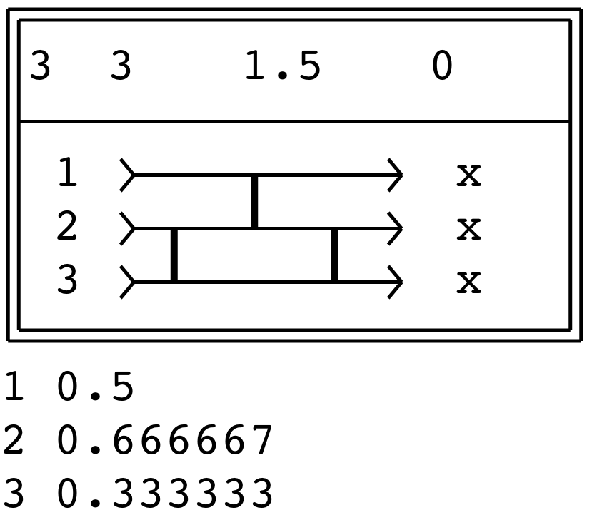
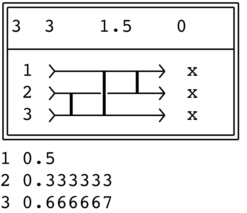
(a)		(b)

Figure 1: Two sorting networks: (a) corresponds to the comparisons (23), (12), (23), at stages 1, 2, 3, respectively; (b) corresponds to the comparisons (23), (13), (12), at stages 1, 2, 3, respectively.

Exchanges are costly, often at a ratio of $2:1$ or $3:1$ to a simple comparison. We have affixed the likelihood of an exchange to each link. Summary statistics give the maximum and average number of exchanges for the entire network. Consider Figure 1(a) which features 3 stages, namely —in that order— (23), (12), and again (23). The number 3 in the upper left corner gives the number of links for this particular network. The second number, again 3 here, means that there is one input to the network where $3$ links are active and swap, the worst-case scenario. The third number, 1.5, means that the average number of swaps, taken over all possible inputs, is $1.5$. The number 0 in the upper right corner is a degree of disorder meaning that this design results in a fully sorted array which can also be seen by the three x characters in the output. Below the left rectangle, the first row “1 0.5” signifies that the probability of an exchange at stage 1 is $0.5=\tfrac{1}{2}$; the second row “2 0.666667” signifies that the probability of an exchange at stage 2 is $0.666667\approx 2/3$; finally, the third row “3 0.333333” signifies that the probability of an exchange at stage 3 is $0.333333\approx 1/3$. In Appendix A, we provide more details on how the statistics in Figure 1(a) was obtained.

The networks presented so far for $N=3$ are distinct and require in both cases three stages, comparisons and exchanges. Both also demonstrate that a full sort network will include all possible $\texttt{length}=1$ links as these alone can serve to reorder permutations of sorted data when merely one adjacent transposition exists. The symmetry in Figure 1(b) is compelling: it allows for fully bidirectional sorting when then input and output sides reverse. Unfortunately, it (as in Figure 1(a)) also exhibits a link (a.k.a. comparator in [4]) in which swapping occurs more often than not.

When a link exchange occurs more than half the time, we may reverse the swap vs non-swap $.67/.33$ to $.33/.67$ by preexchanging its elements. We remove the direct cost of the exchange by reversing the order of input lines to the left of the offending link. But all inputs are unsorted so any non-conditional exchange has no sorting efficacy and may be removed. In Figure 1(a), the offending link is at stage 2, namely (12). Thus, we replace (23) by (13) at stage 1 while keeping (23) at stage 3 unchanged. For Figure 1(b), the offending link is at stage 3, namely (12). Thus, we replace (23) by (13) at stage 1 and (13) by (23) at stage 2.

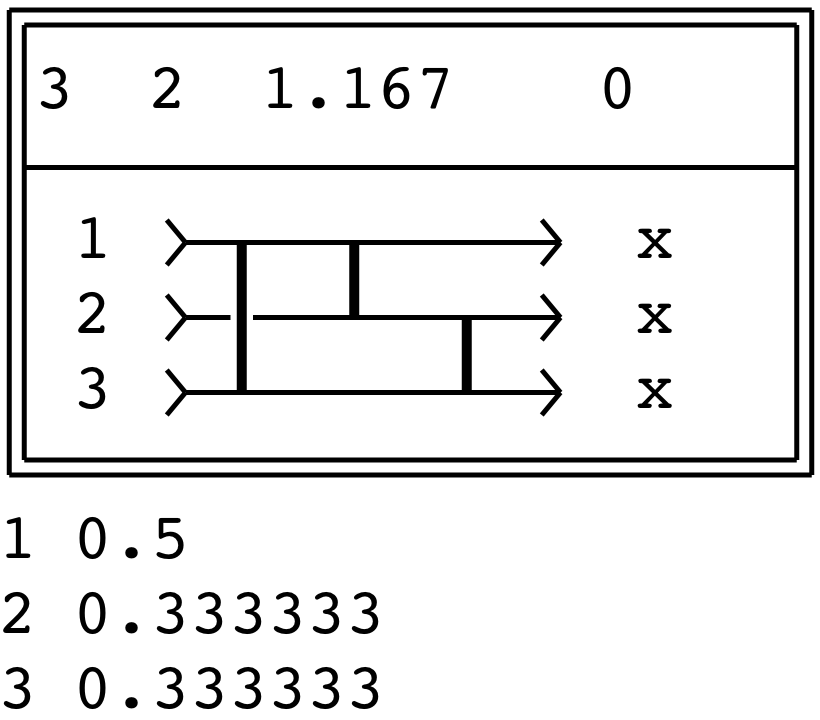
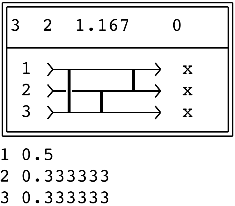
(a)		(b)

Figure 2: Two sorting networks: (a) corresponds to the comparisons (13), (12), (23), at stages 1, 2, 3, respectively; (b) corresponds to the comparisons (13), (23), (12), at stages 1, 2, 3, respectively.

The networks, depicted in Figure 2 and identical under mirror symmetry, substantially improve the average cost of exchange. More striking is a reduction in maximum exchange, which was lowered from 3 to 2! Moreover, the average number of swaps was lowered from $3/2=1.5$ to $7/6\approx 1.167$. This is unexpected and serves as the basis of non-interfering concurrent exchange. Clearly, the first link may exchange without restriction. The remaining cost of one exchange must be shared between the two remaining links: at most one may occur. This in turn implies that the central element cannot be rewritten by both links, allowing both the upper and lower link concurrent execution.

We now create a new fused dual-link element, which we name a “2-op” (borrowing from mathematical nomenclature used for such occurrences), depicted below:

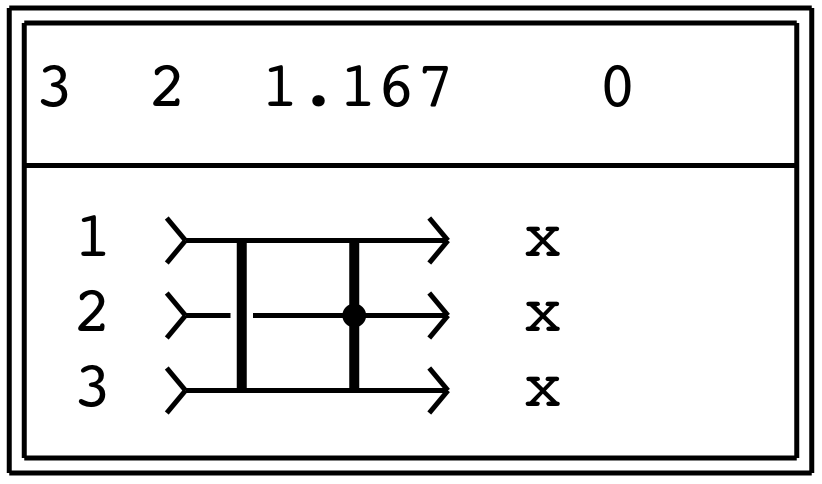
Figure 3: At stage 1, we have the comparison $(13)$, while at stage 2, we have the new 2-op $(123)$ which will execute at most one of the exchanges $\{(12),(23)\}$.

The circle at the common link joint $2$ indicates non-interference.

2 9-element networks and medians

The 2-op exchange on three elements yields immediate gains in lowering costs of traditional networks. For example, Paeth [5] described a median on a $3\times 3$ box (see Figure 4),

1	2	3
4	5	6
7	8	9

Figure 4: Labeling of cells in the $3\times 3$ box.

formed by column, row and (single) diagonal sorting, first conceived as a means to reuse column sorts when filtering a large raster image.

Defining $\operatorname{s3}(a,b,c)$ to be either the three swaps $(a,b)(b,c)(a,b)$ (as in the original [5]) or $(a,c)(a,b)(b,c)$ (reworked to be a 2-op!), we can find the median by $\operatorname{s3}(1,4,7)$, $\operatorname{s3}(2,5,8)$, $\operatorname{s3}(3,6,9)$, $\operatorname{s3}(1,2,3)$, $\operatorname{s3}(4,5,6)$, $\operatorname{s3}(7,8,9)$, $\operatorname{s3}(3,5,7)$, where this sequence of operators is executed from left to right.

2.1 Original design

The first version gives the 21-link network in Figure 5 below.

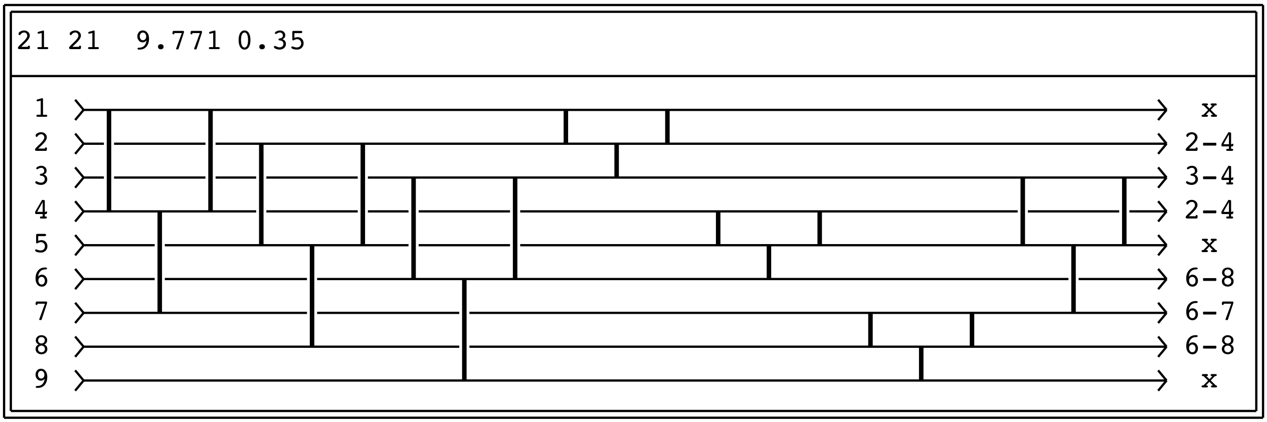
Figure 5: A 21-link network to determine the median. The probabilities of swapping are: $\nicefrac{{1}}{{2}}$ at link 1, $\nicefrac{{2}}{{3}}$ at link 2, $\nicefrac{{1}}{{3}}$ at link 3, $\nicefrac{{1}}{{2}}$ at link 4, $\nicefrac{{2}}{{3}}$ at link 5, $\nicefrac{{1}}{{3}}$ at link 6, $\nicefrac{{1}}{{2}}$ at link 7, $\nicefrac{{2}}{{3}}$ at link 8, $\nicefrac{{1}}{{3}}$ at link 9, $\nicefrac{{1}}{{2}}$ at link 10, $\nicefrac{{2}}{{3}}$ at link 11, $\nicefrac{{1}}{{3}}$ at link 12, $\nicefrac{{1}}{{2}}$ at link 13, $\nicefrac{{2}}{{3}}$ at link 14, $\nicefrac{{1}}{{3}}$ at link 15, $\nicefrac{{1}}{{2}}$ at link 16, $\nicefrac{{2}}{{3}}$ at link 17, $\nicefrac{{1}}{{3}}$ at link 18, $\nicefrac{{19}}{{70}}$ at link 19, $\nicefrac{{5}}{{14}}$ at link 20, $\nicefrac{{1}}{{7}}$ at link 21. This results in $9\nicefrac{{27}}{{35}}\approx 9.771$ swaps on average.

In Figure 6, we re-arrange the links in Figure 5 to highlight stages, i.e., links that can be executed in parallel. (Stages correspond to delay time in [4].) This does not change the overall swap statistics:

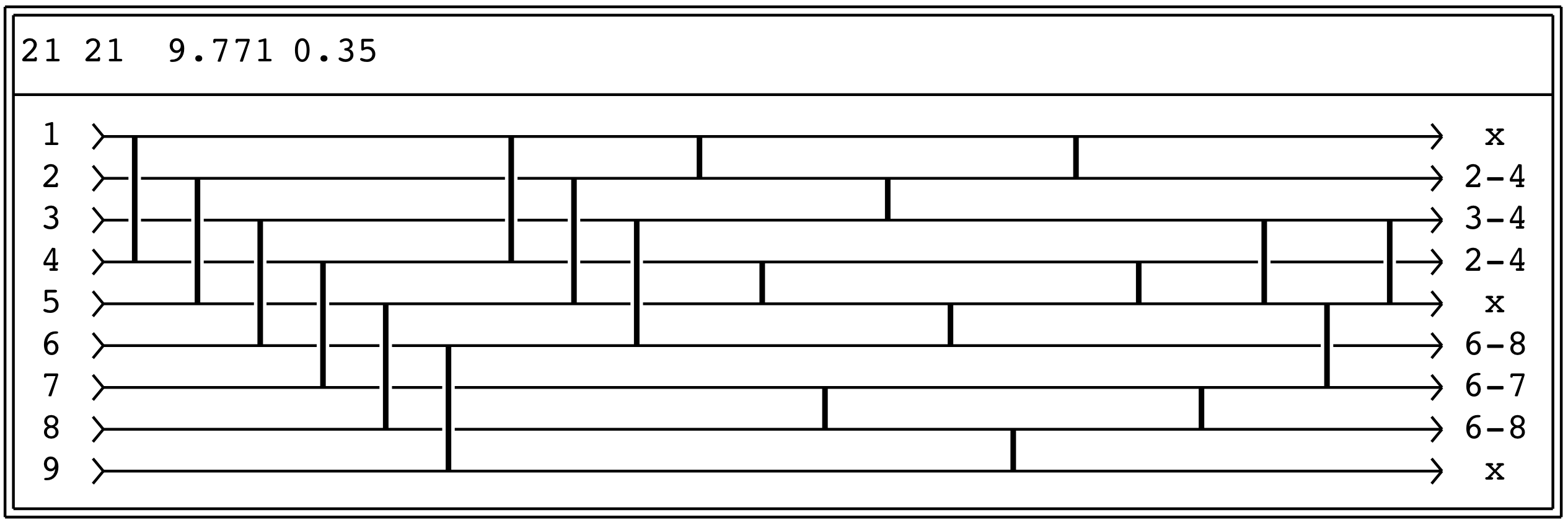
Figure 6: The 21-link network to determine the median from Figure 5 re-arranged. Note that there are 9 stages (stage 1: links $(1,4)(2,5)(3,6)$; stage 2: links $(4,7)(5,8)(6,9)$; stage 3: links $(1,4)(2,5)(3,6)$; stage 4: links $(1,2)(4,5)(7,9)$; stage 5: links $(2,3)(5,6)(8,9)$; stage 6: links $(1,2)(4,5)(7,9)$; stage 7: link $(3,5)$; stage 8: link $(5,7)$; stage 9: link $(3,5)$) that can be executed in parallel.

Using 21 links, we find minimum, maximum and median (see Figure 5 or Figure 6 above.) This design leads to efficient bare median (19 links) and full sorting (25 links) on nine-element arrays; see Figure 7 below.

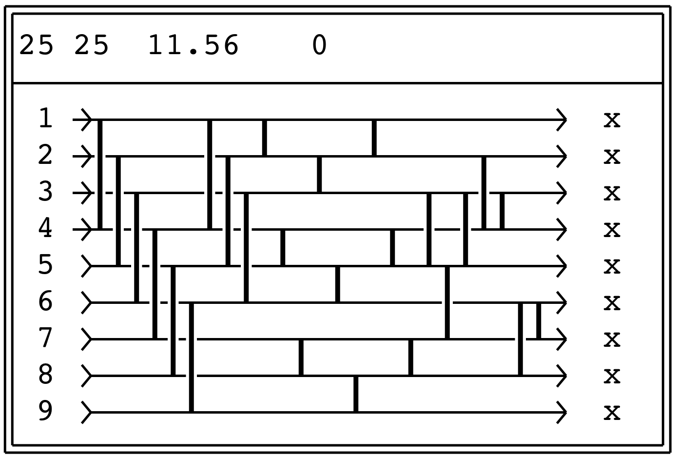
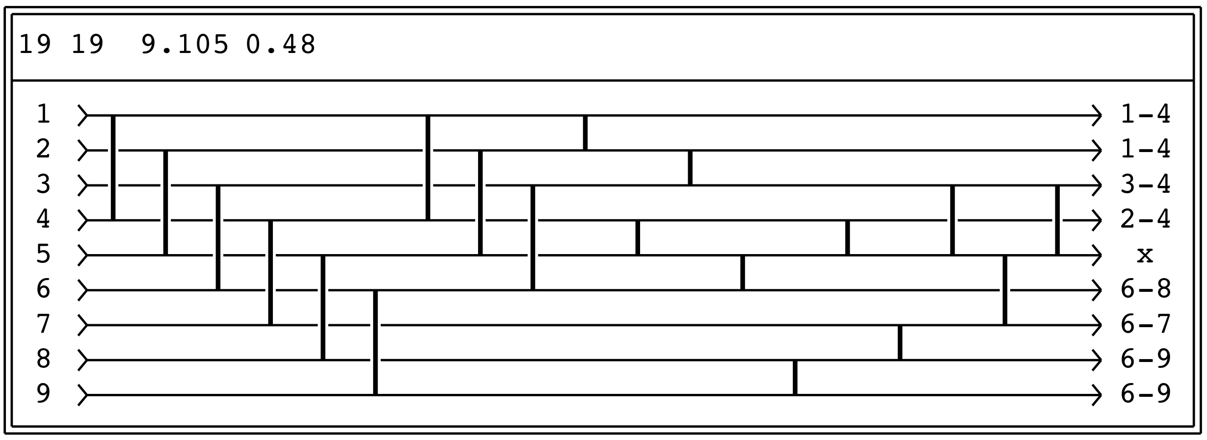
(a)		(b)

Figure 7: Two sorting networks derived from that in Figure 6. (a) corresponds to the fully sorted version by adding the links $(23),(34),(68),(67)$ at the end. (b) corresponds to the bare median version by deleting the first $(1,2)$ link and the last $(7,8)$ link.

Exchanges on 21 links occur when presented reverse sorted input, and (see Figure 5) $9\nicefrac{{27}}{{35}}\approx 9.771$ times on average which gives a relative frequency of $(9\nicefrac{{27}}{{35}})/21=\nicefrac{{114}}{{245}}\approx 47\%$.

2.2 New design using 3-ops

Substitution of $\operatorname{s3}$ by its reworked 3-op version gives the network in Figure 8 below.

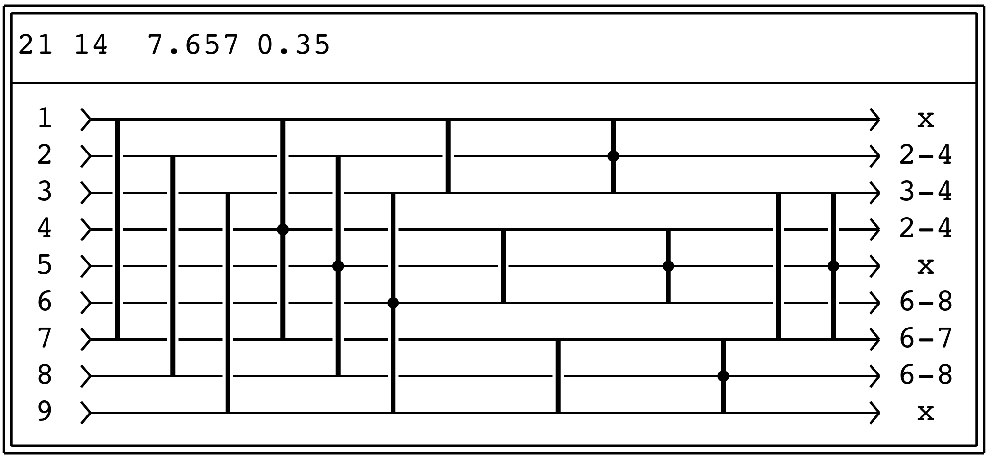
Figure 8: A new network based on 3-ops, featuring 6 stages.

Full sorting in 25 links adds the four CE elements $(2,4)(3,4)(6,8)(6,7)$; Bare median finding in 19 links omits $(1,2)$ and $(8,9)$ from the 2-ops $(1,2,3)$ and $(7,8,9)$, respectively. Note that these omissions cannot be made directly on the original net without permutations to allow for median. The final networks are presented in Figure 9 below.

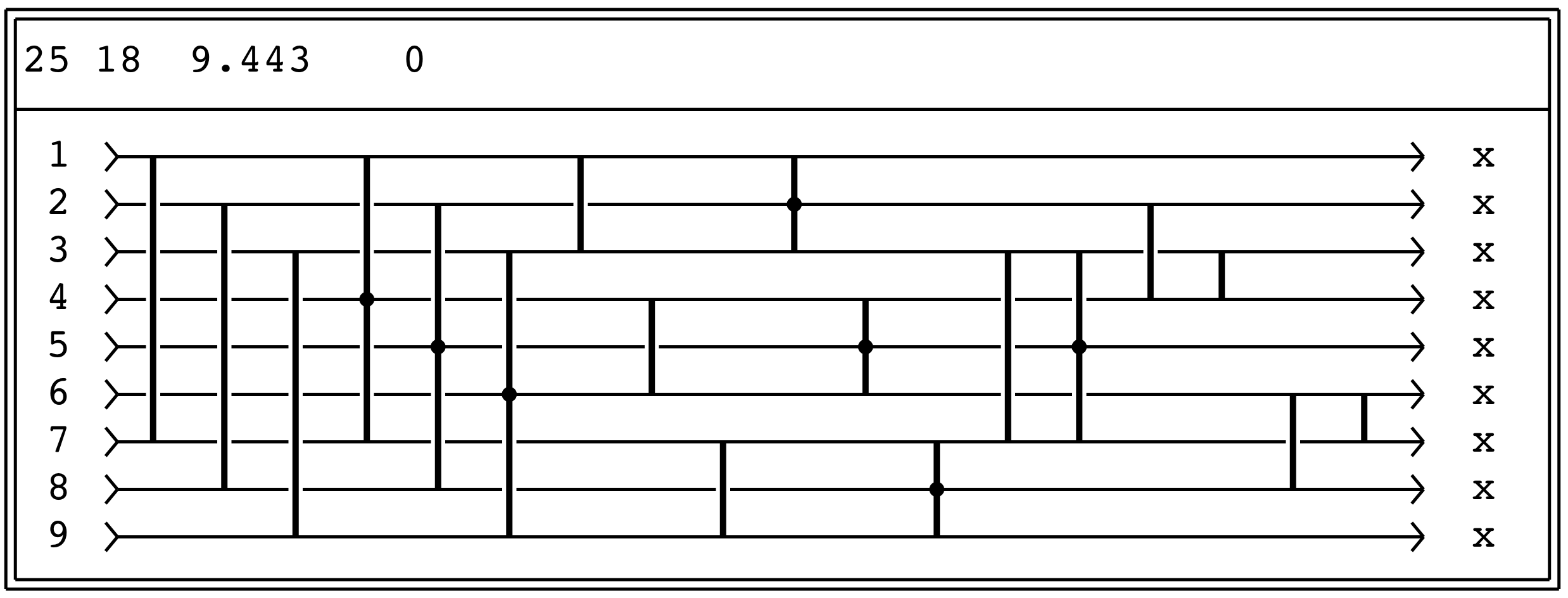
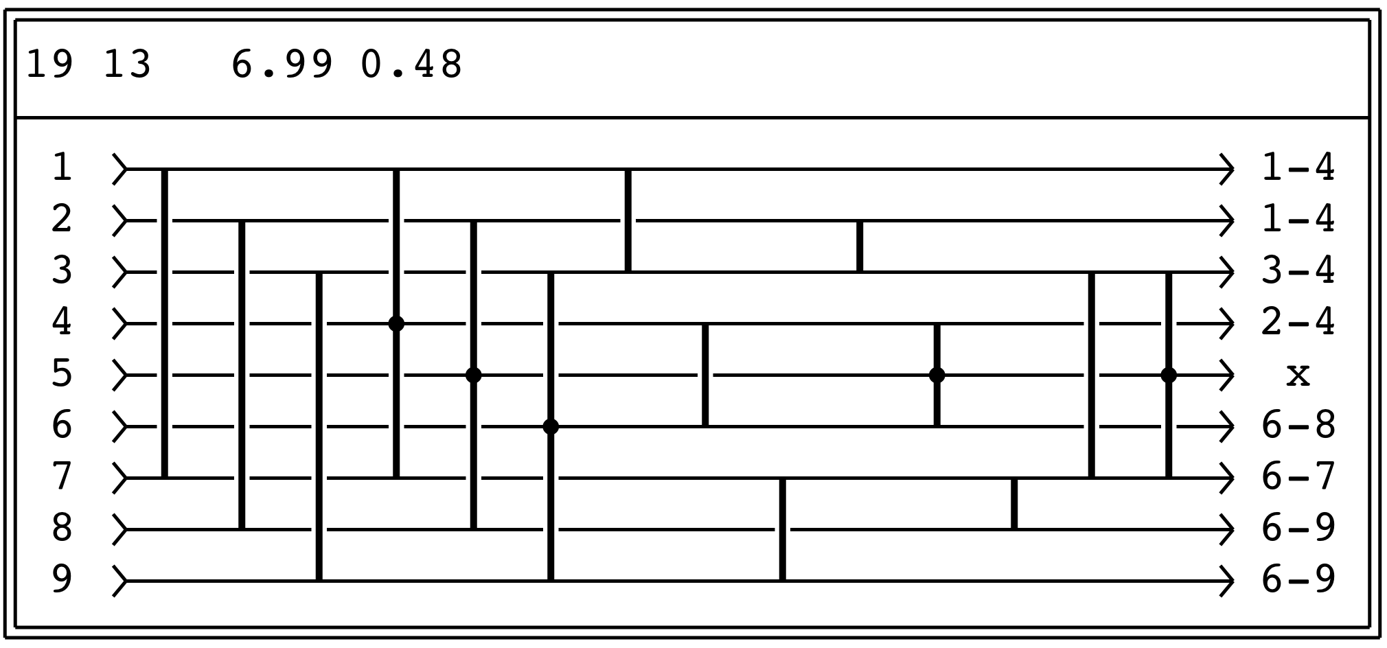
(a)		(b)

Figure 9: Two sorting networks derived from that in Figure 8. (a) corresponds to the fully sorted version by adding the links $(23),(34),(68),(67)$. (b) corresponds to the bare median version by deleting the links $(1,2)$ and $(8,9)$ from the 2-ops $(1,2,3)$ and $(7,8,9)$ respectively.

2.3 Comparison

We summarize the benefits of the new design versus the old design in Table 1:

Design	Median only				Min/Med/Max				Fully sorted
	Swaps		Stages		Swaps		Stages		Swaps		Stages
	Avg	Max			Avg	Max			Avg	Max
old	9.105	19	9		9.771	21	9		11.56	25	11
new	6.99	13	6		7.657	14	6		9.443	18	8
new/old	76.8%	68.4%	66.7%		78.4%	66.7%	66.7%		81.7%	72.0%	72.7%

Table 1: Summarized statistics of the old and the new design for sorting $9$-element networks.

We conclude our discussion by listing Schwiebert’s sorting network which is known to have the minimum number of stages/delay time. Note that the average and maximum number of comparisons is considerably higher.

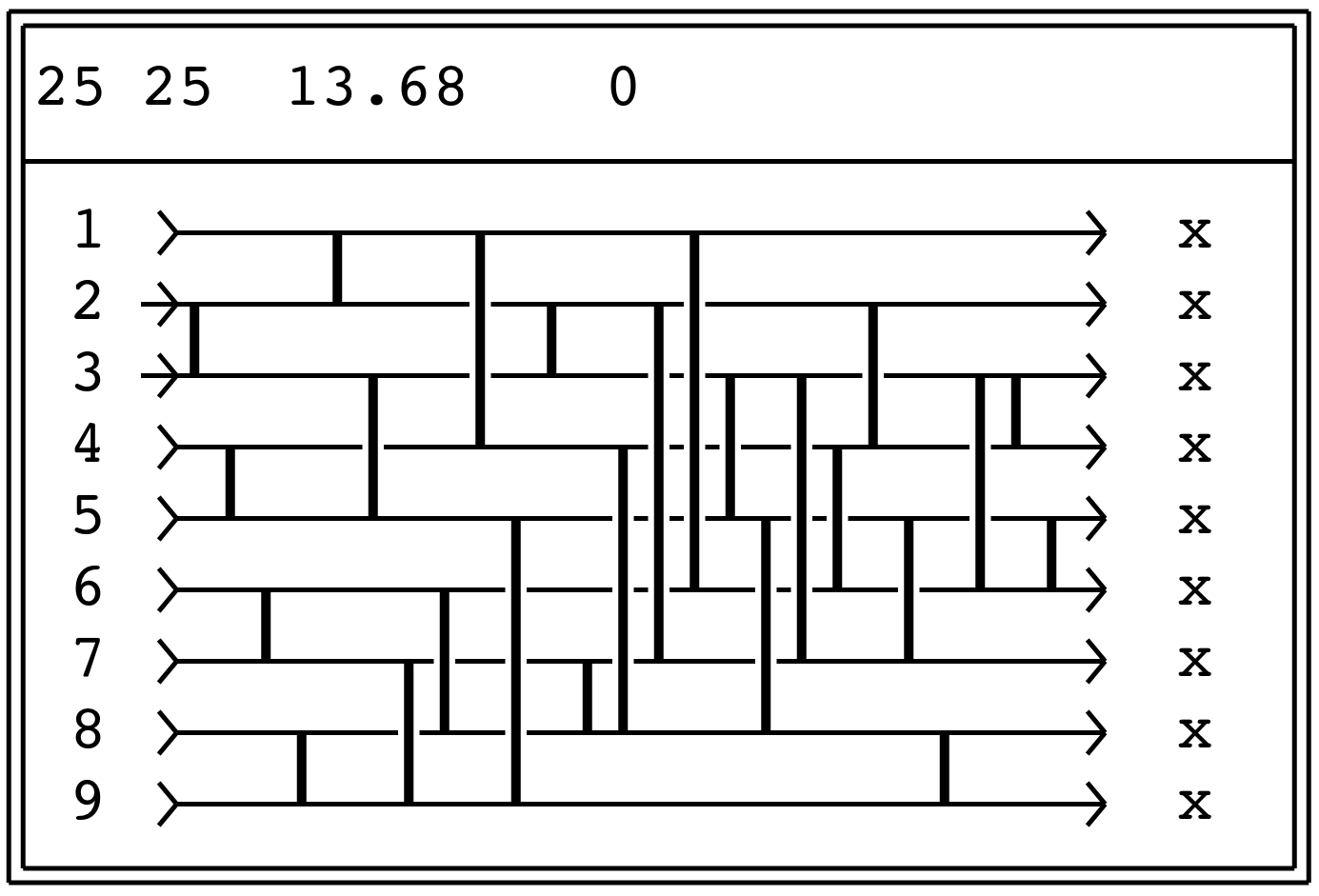
Figure 10: Loren Schwiebert’s 25-link sorting network for 9 elements taken from [4, Figure 51 for $n=9$] with delay time $7$, i.e., $7$ stages.

3 Intuition and Extension

To some the lowered statistics seem surprising. Typical reasoning follows: ”to sort three, order any two, the third draws a bye. Bye enters and plays to establish an overall winner (WLOG, loser); third step ranks the runner’s up.” While accurate when elements are chosen freely, as a memory-based method each element carries a rank implicit in its index. CE sorting ranks all elements, chosen pairs are not isomorphic. In the case of $N=3$ we may disambiguate thus: “Choosing any two at most omits the median, our set is are guaranteed to hold at least the min or max. Choosing and sorting the outermost elements therefore guarantees at least one of max or min landing in its final position. A single swap will place the remaining extrema; both extreme must be treated (a 2-op). With both extrema placed, median is properly placed by process of elimination”.

Students of computer science will recognize Figure 1(a) as bubble-sort on three elements where the initial link leaves the maximum element in central position $2/3$ of the time (for the remaining $1/3$, it started in proper position and will not move), thereby encumbering subsequent links the task of floating it into its outer position. By comparison, the non-interfering method is seen as a selection or insertion sort whose improved swapping statistics are well-known. It is ironic such study of CE networks is rare and that the total number of links (or stages) has remained the sole performance metric for so long.

Conceptually, the longer prefacing element link in Figure 2(a) serves as a guard in assuring that no double-exchange occurs, allowing fusion into one 2-op. The final links might not be unit length, as seen in the improved sort/median on nine elements. The guard needs only protect (operate on) the outer two unshared elements. As a second and more interesting means of extension, we envision a 3-op of higher order, formed by allowing two adjacent 2-ops to execute concurrently. We explore the latter now.

4 Sorting $N=4$

A trial network (see Figure 11(a)) overlaps two optimal 3-sorts, sharing a central element, whose sorting statistics and testing reveal a maximum swap of four elements, occurring only with the center link $(2,3)$ of the 3-op $(1,2,3,4)$, which consists of 3 links without conflict: $(1,2)$, $(2,3)$, and $(3,4)$ where $(2,3)$ is either non-active or the only active link. Unfortunately, this network fails to fully sort in five steps: $1/6$ of the time, the central elements are transposed, requiring a sixth link as seen in Figure 11(b). This is both undesirable and surprising: the final link seemingly replicates the work concluded immediately its left. There are two remedies to this. Both rely on the fact that the central link in the 3-op might not execute, yet its operation is essential to attain a full sort.

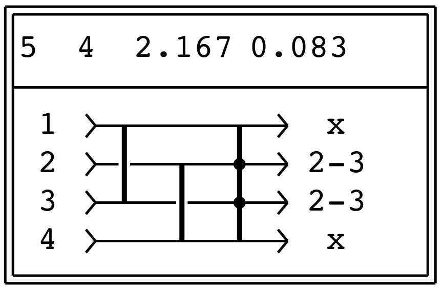
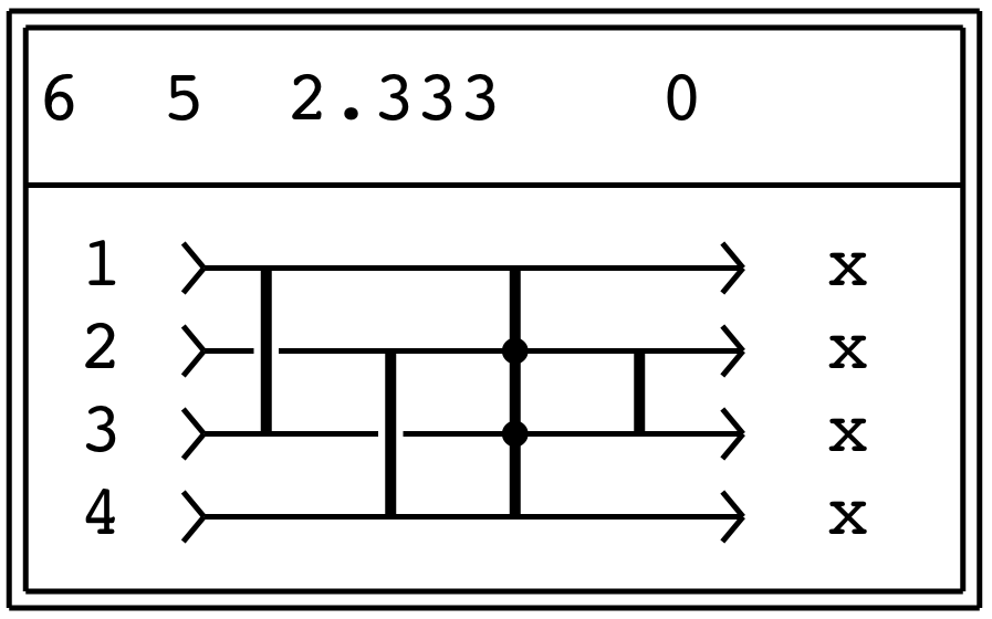
(a)		(b)

Figure 11: A sorting network for $N=4$ identifying min/max in (a) on the left, and fully sorting in (b) on the right.

Our first solution breaks the 3-op into its constituent links. Since they do not interfere, we are afforded any ordering of its components. We first choose to place the link to its right, giving rise to redundant right-most central links (not shown). We retain one only, giving the familiar solution Figure 12(a), sans N-ops. The second solution, depicted in Figure 12(b), recognizes that the additional link is necessary in the case the 3-op is fully active (i.e., two outer swaps), its actions then juxtaposing two (as yet unordered) elements against each other into adjacent central position. As before, we guard against interference by employing a prefacing link whose two endpoints are the outer endpoints (elements) of the two links it protects.

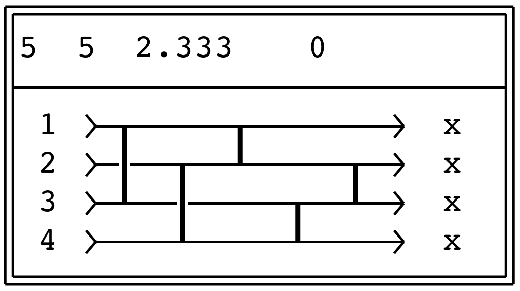
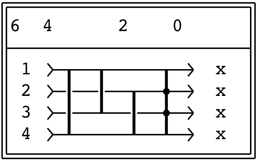
(a)		(b)

Figure 12: (a): Swap frequencies are $\nicefrac{{1}}{{2}}$ at links 1,2,3,4; $\nicefrac{{1}}{{3}}$ at link 5. (b): Swap frequencies are $\nicefrac{{1}}{{2}}$ at link 1; $\nicefrac{{1}}{{3}}$ at links 2 and 3; $\nicefrac{{1}}{{4}},\nicefrac{{1}}{{2}},\nicefrac{{1}}{{4}}$ at $(1,2),(2,3),(3,4)$ from the 3-op $(1,2,3,4)$, respectively.

The second solution (in Figure 12(b)) is in fact the $\mathcal{O}(n^{2})$ pair-wise comparison of all elements, taken in descending order, which necessarily ranks all elements. While not a viable solution for large $N$, for $N=4$ it sits close to the theoretical minimum (5 links, see Figure 13 below) and rewards the implementor with surprisingly good statistics for average swaps (2) while nonetheless executing in at most three hardware stages.

Large networks whose size $N$ is a power of two, have many prefacing links whose sorting statistics show a $50/50$ probability of exchange. The transposition operator may be applied to any such link (and to any implicated links lying to its left) without changes to the average sorting statistics. The topological change may instead succeed in reducing the maximum number of exchanges. Applied to the network seen in Figure 12(a), we obtain the network depicted in Figure 13 below, where the maximum number of exchanges dropped from 5 to 4.

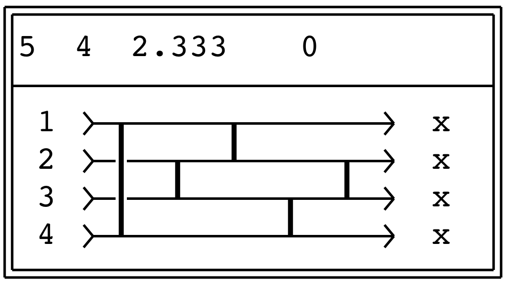
Figure 13: A 5-link sorting network for 4 elements. The last link has swap probability of $\nicefrac{{1}}{{3}}$; all other links have swap probability of $\nicefrac{{1}}{{2}}$.

The worst-case input occurs when reordering $(3,4,1,2)$ and in this case all save but the final link are active. A breakdown of total swap counts appears below:

Figure 14: A histogram for representing the number of occurrences with respect to number of exchanges/swaps required for all possible inputs for the two networks from Figures 12(a) and Figure 13. The input requiring 5 exchanges for the network from Figure 12(a) is $(4,2,3,1)$.

Note that the reappearance of the central link $(2,3)$ in Figure 13 implies that a ”needless” i.e. redundant comparison might take place, as when presented the input $(1,3,2,4)$ requiring merely one central transposition. This cannot be helped; the network is statistically optimal. In the extreme case, sorted data requiring no exchanges will nonetheless compare at all link positions, including ”redundant” links – such is the topology of CE networks. Attempts to mitigate this, such as (software) early termination as when reaching the threshold of maximum exchange are not cost effective: they must both count and test in order to detect this condition at a cost often greater than a few additional link comparisons.

The network depicted in Figure 13 also sheds light into the subtleties of conditional probability. While there are $4!=24$ possible inputs permutations, the first four links cannot each successively half the size of the solution space: $24$ is not divisible by $2^{4}=16$. While links 3 and 4 both execute independently with $50/50$ exchange statistics, they are nonetheless conditionally bound. If link 3 does execute, then there is a $\nicefrac{{2}}{{3}}$ chance that link 4 does not, and vice versa. In effect, when ”double winner” (max of all four) is found by exchanging element 2 with 3, previous losers to this element may be ascribed less demotion; they are more apt to retain a superior position and not trigger a link 4 exchange. Intuition aside, careful analysis of exchange statistics bears this all out.

Finally, we compare the network in Figure 13 to the following one found in [4, Figure 44]:

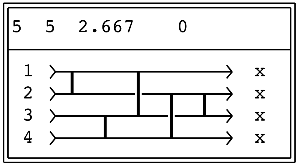
Figure 15: A 5-link sorting network for 4 elements taken from [4, Figure 44]. The last link has swap probability of $\nicefrac{{2}}{{3}}$; all other links have swap probability of $\nicefrac{{1}}{{2}}$.

Note that this network does not compare as well as the one in Figure 13; it requires 5 swaps and the average number of swaps is higher as well.

5 Software Implementation

Reduction in total exchanges without the use of conditional directives is the greatest benefit of CONEX techniques. In the case of 2-ops and 3-ops a simple software addition can reduce the explicit cost of an unnecessary comparison:

  #define sort2(a,b)   if ((a) < (b)) { (a) ^= (b); (b) ^= (a); (a) ^= (b) }
  #define op2(a,b,c)   if (sort2(a,b)) else sort2(b,c)
  #define sort3(a,b,c) sort2(a,c); op2(a,b,c)

in which the ”else” elides a non-interfering CE element. The form shown above provides exchanges without resort to additional variables / registers. If we allow their inclusion the difference implicit in the first comparison can be retained to speed the body of the exchange, as shown elsewhere [5].

  #define sort2(a,b)   if ((t = (a) - (b)) < 0) { (b) += t; (a) -= t); }

With 3-ops, an exchange of the central element will elide possible swaps by the outlying “wings”

  #define op3(a,b,c,d)   if (sort2(b,c)) else { sort2(a,b); sort2(c,d); }

These macros expand as in-line code, removing subroutine overhead and form the basic primitives used in software implementations of NICE networks.

6 Higher Order Networks

For $N$ odd, we explore methods of median finding, for $N$ even, we consider fully sorting networks.

6.1 Sorting $N=5$

An efficient method for $N=5$ is elusive: network sizes which are a power of two show a high degree of symmetry, sizes $2^{n}+1$ must accommodate the new addition. Theory prescribes 7 comparisons (as $5!=120<128=2^{7}$), and is realizable in careful practice. For CE implementations, a worst case figure of 10 links is an upper bound, this is the triangle number $T(4)=4(4+1)/2$ enumerating all pairwise comparisons of five elements. In practice, nine links is the minimum CE implementation. Exhaustive searching reveals that a simple elimination of one maximal element (four steps) followed by a sort4 (five links) gives the best sorting statistics:

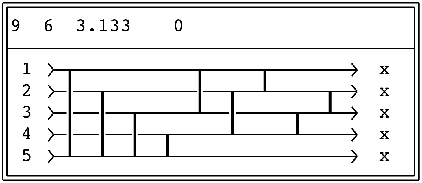
Figure 16: A 9-link network to sort 5 elements. The probabilities of swapping are: $\nicefrac{{1}}{{2}}$ at link 1, $\nicefrac{{1}}{{3}}$ at link 2, $\nicefrac{{1}}{{4}}$ at link 3, $\nicefrac{{1}}{{5}}$ at link 4, $\nicefrac{{1}}{{3}}$ at link 5, $\nicefrac{{5}}{{12}}$ at link 6, $\nicefrac{{2}}{{5}}$ at link 7, $\nicefrac{{2}}{{5}}$ at link 8, $\nicefrac{{3}}{{10}}$ at link 9. This results in $3\nicefrac{{2}}{{15}}=3.1\overline{3}$ swaps on average.

Note that the final sort is of the style of that one in Figure 12(a), and not the one in Figure 13. While not strictly a NICE network, a compact software implementation for $N=5$ is a good project for future work.

6.2 Sorting $N=6$

For $N=6$, three-sort the elements $(1,3,5)$ and symmetrically on $(2,4,6)$, after sorting $(1,5)$ and $(2,6)$. Note that in each case a central 2-op occurs on element 3 (4). We now center these two elements by again using a 2-op, but this time against the outer interval formed by the opposing 3-sort; that is, the 2-ops $(1,4,5)$ and $(2,3,6)$. These leads to a highly parallel execution model in which the central two elements are located at $(3,4)$ albeit unordered. By the ranking nature of CE networks, elements $(1,2)$ and $(5,6)$ are also properly partitioned, albeit unsorted. Three concurrent links at $(1,2)$, $(3,4)$ and $(5,6)$ thereby conclude the sort (see Figure 17):

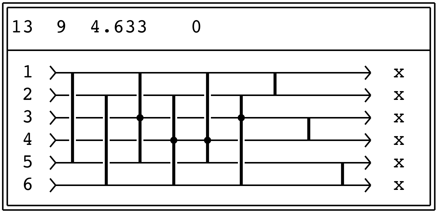
Figure 17: A network to sort $6$ elements.

A rework of the network from Figure 17 presented in Figure 18 preserves the overall exchange statistics while lowering the worst-case performance to 8 swaps.

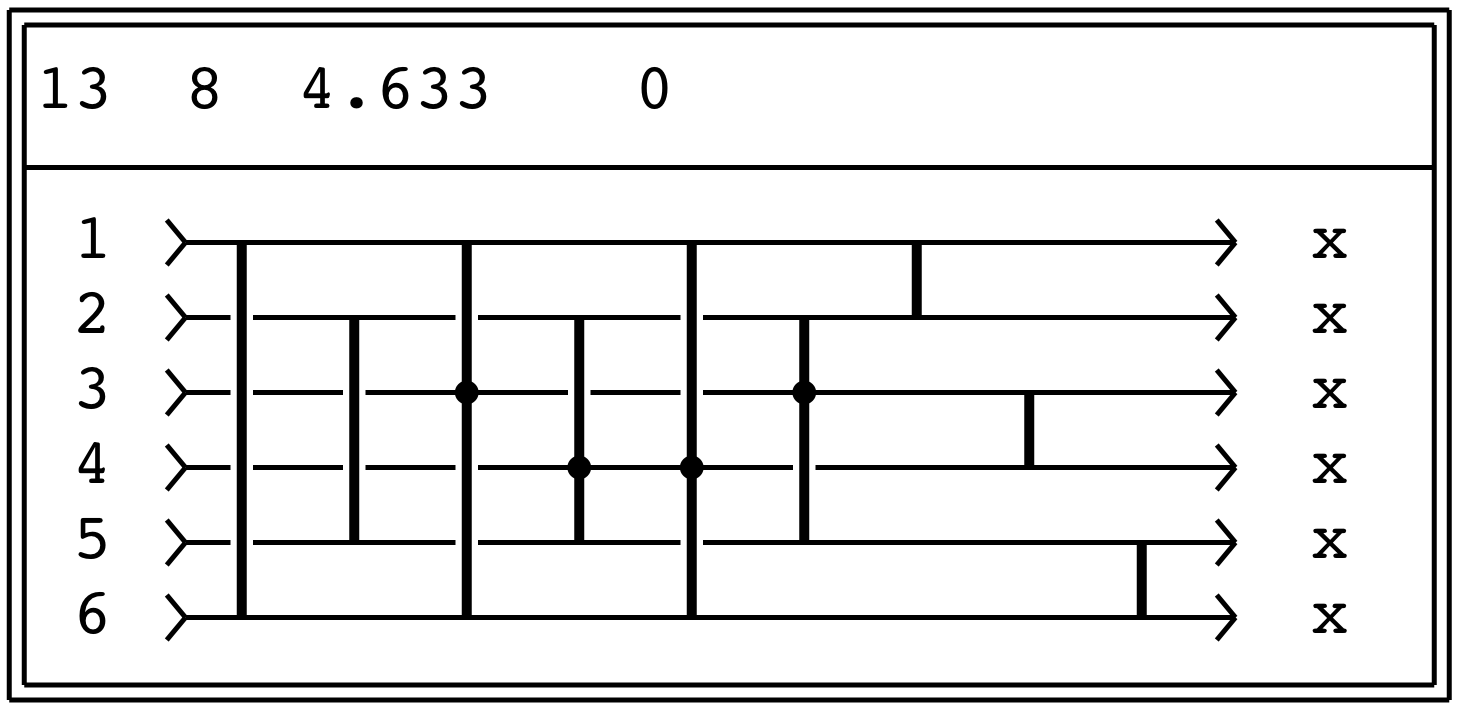
Figure 18: A rework of the network from Figure 17 to sort $6$ elements with improved worst-case performance.

Note that both networks complete in only four stages with the two central stages involving all elements concurrently.

If the goal is to reduce average swaps in reduced links, the network in Figure 19 will do that, at the expense of additional stages:

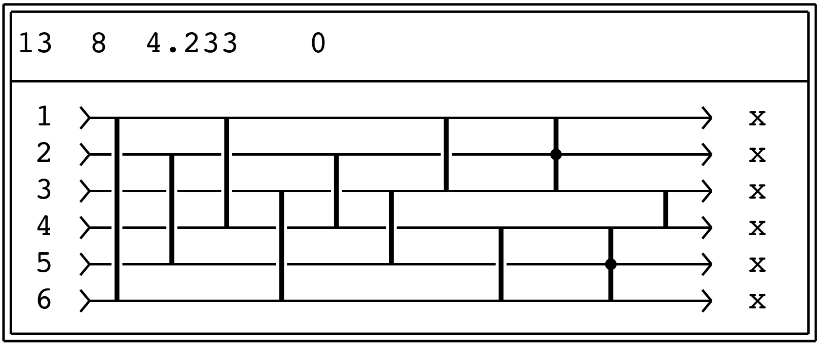
Figure 19: A network to sort $6$ elements with minimum average-swap performance.

Applying basic techniques (symmetric min/max, applied successively) leads to the network depicted in Figure 20 which sorts six elements in just 12 links – the minimum:

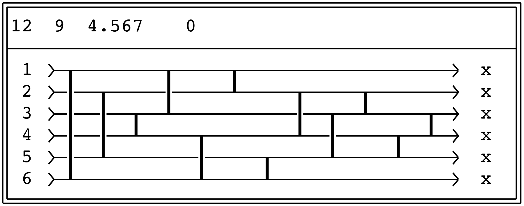
Figure 20: A network to sort $6$ elements with the minimum number (12) of links.

The user may achieve the smallest total number of swaps (8 compared to 9) at the cost of a slightly increased average number of swaps. (This trade-off with mild change in topology symmetry is seen with large networks in general.)

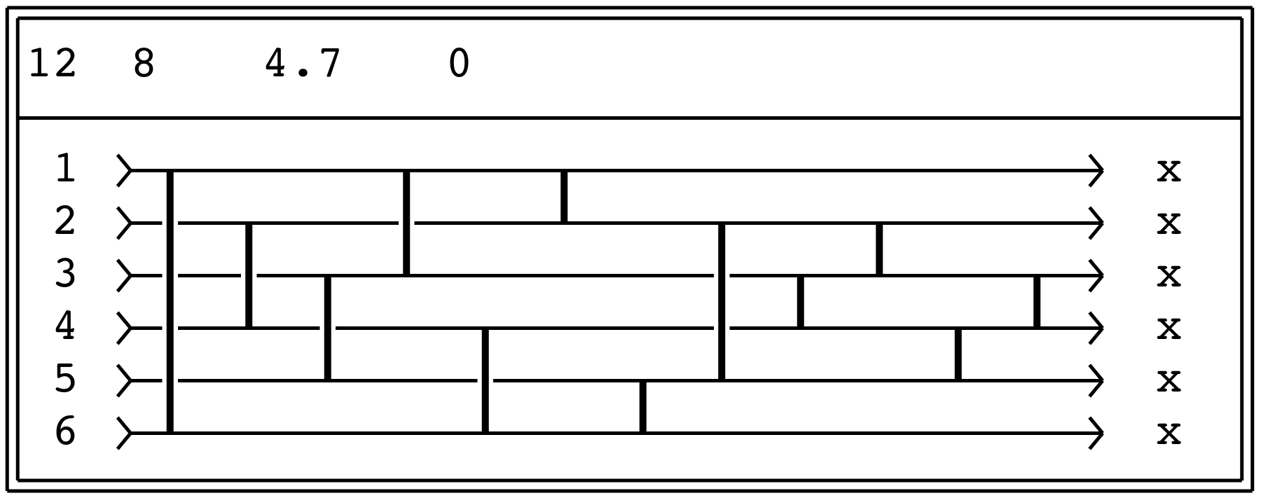
Figure 21: Another network to sort $6$ elements with the minimum number (12) of links but reduced worst-case scenario at the cost of slightly worse average swap performance.

Finally, let us now present Gerald Norris Shapiro’s network (taken from [4, Figure 51]) for sorting six elements in Figure 22:

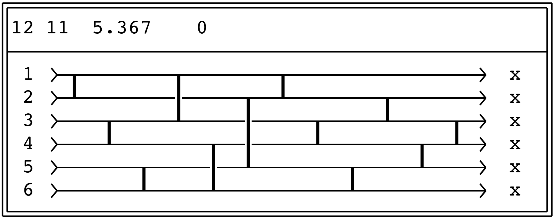
Figure 22: Shapiro’s network for sorting six elements, requiring 5 stages and 12 links.

Given the minimum number of links (12), Shapiro’s network has the minimum number of stages (5); however, in terms of worst case scenario and average number of swaps, the networks in Figure 20 and Figure 21 do better at the expense of just one more stage.

6.3 Sorting $N=7$

In this section, we describe three networks for $N=7$. We start with two networks for determining the median of $7$ elements. Figure 23 is a network for finding the median of $7$ numbers, requiring a low average of only $3.481$ exchanges.

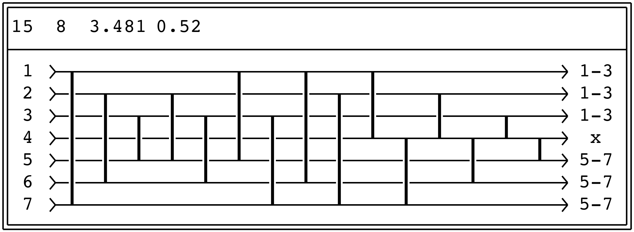
Figure 23: A network to determine the median of $7$ elements, with a low average of $3.481$ exchanges.

The network in Figure 23 has 15 links. The network in Figure 24 finds the median with only 13 links, albeit increasing the average of exchanges to $4.49$.

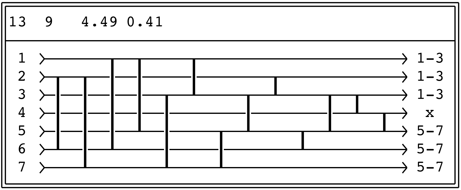
Figure 24: A network to determine the median of $7$ elements, with a low number of 13 links.

We now turn to fully sorting 7 elements. The network in Figure 25 has a low average of $5.271$ exchanges:

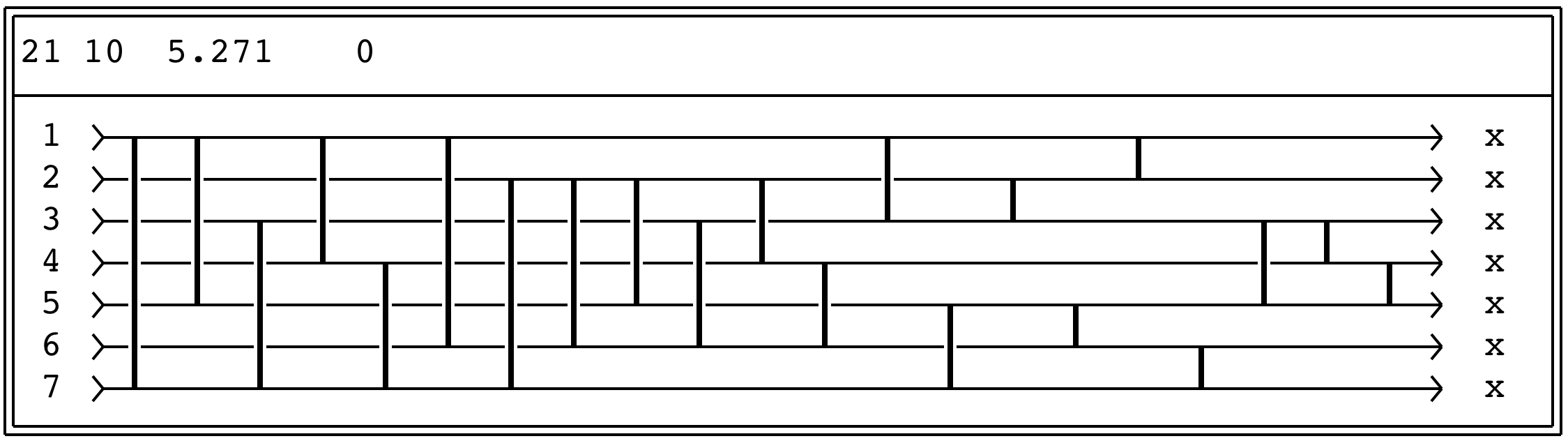
Figure 25: A network to fully sort $7$ elements, with a low average of $5.271$ exchanges.

6.4 Sorting $N=8$

We start with the classical Batcher’s odd-even mergesort [2], for sorting 8 elements:

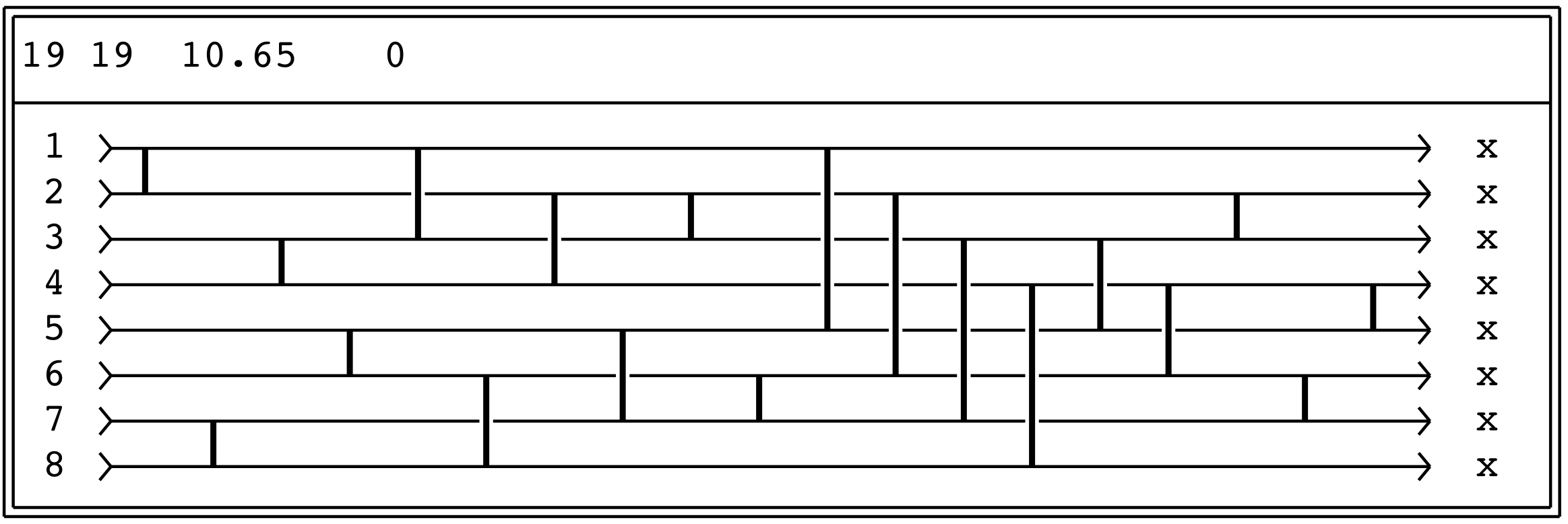
Figure 26: Batcher’s classical odd-even mergesort requires 19 links to sort eight elements.

Batcher’s network is known to realize the minimum number of links, 19. However, we now present two networks with the same number of links, but with much improved statistics. First, the network in Figure 27 has a much improved average number of exchanges, $7.933$ vs Batcher’s $10.65$ and the maximum number of swaps is only 15 vs Batcher’s 19.

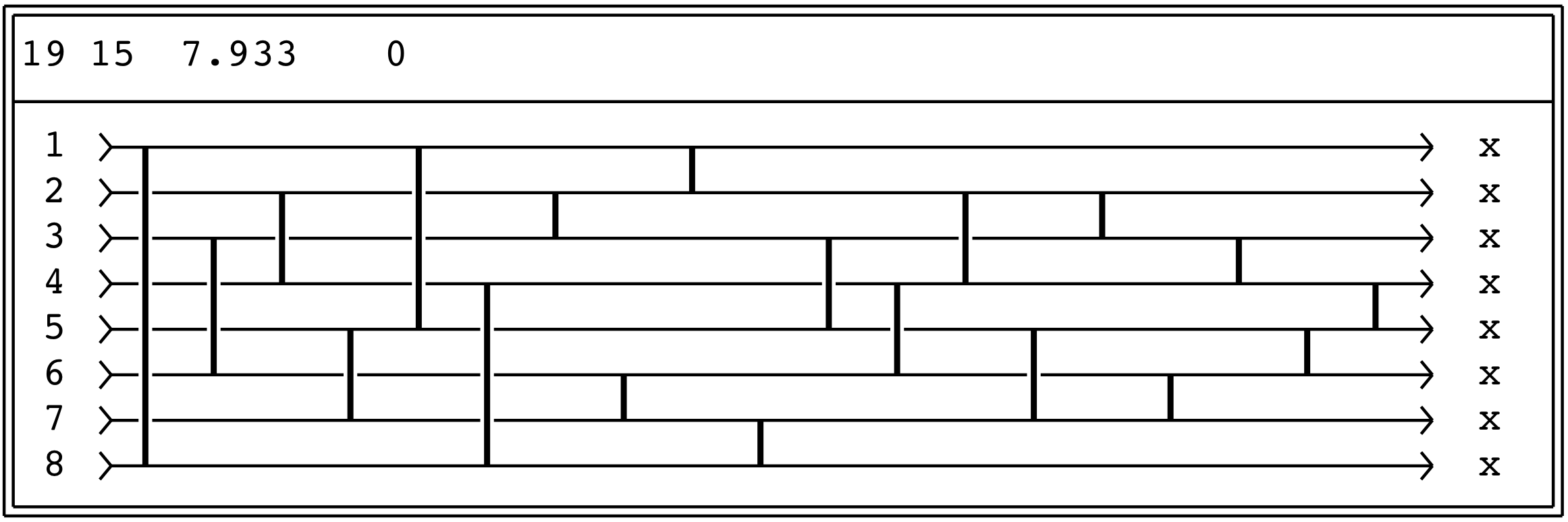
Figure 27: A network to fully sort $8$ elements, with a low average of $7.933$ exchanges.

Second, the network in Figure 28 has a maximum number of swaps of only 14 compared to Batcher’s 19.

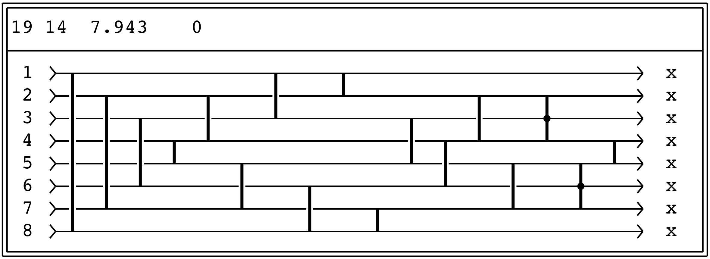
Figure 28: A network to fully sort $8$ elements, with a low maximum number of swaps of $14$.

We conclude in Figure 29 with a network with an even lower maximum number, namely 12, albeit with 28 links:

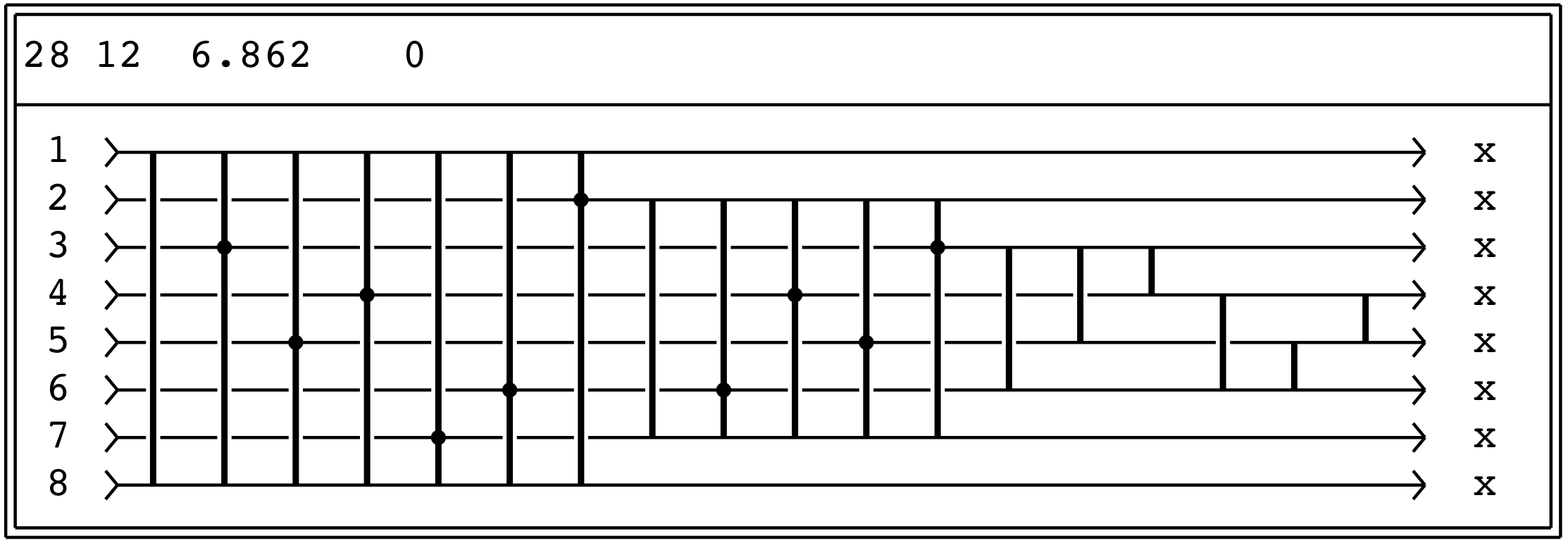
Figure 29: A network to fully sort $8$ elements, with a low maximum number of swaps of $12$.

Appendix A

Memory contents
Stage 0	Stage 1	Stage 2	Stage 3	Number of
(initial)	(2–3 swap)	(1–2 swap)	(2–3 swap)	swaps
$(1,2,3)$	$(1,2,3)$	$(1,2,3)$	$(1,2,3)$	0
$(1,3,2)$	$(1,\mathbf{2},\mathbf{3})$	$(1,2,3)$	$(1,2,3)$	1
$(2,1,3)$	$(2,1,3)$	$(\mathbf{1},\mathbf{2},3)$	$(1,2,3)$	1
$(2,3,1)$	$(2,\mathbf{1},\mathbf{3})$	$(\mathbf{1},\mathbf{2},3)$	$(1,2,3)$	2
$(3,1,2)$	$(3,1,2)$	$(\mathbf{1},\mathbf{3},2)$	$(1,\mathbf{2},\mathbf{3})$	2
$(3,2,1)$	$(3,\mathbf{1},\mathbf{2})$	$(\mathbf{1},\mathbf{3},2)$	$(1,\mathbf{2},\mathbf{3})$	3
Number of swaps	3	4	2	9

Table 2: The behaviour of the network from Figure 1(a).

Memory contents
Stage 0	Stage 1	Stage 2	Stage 3	Number of
(initial)	(1–3 swap)	(1–2 swap)	(2–3 swap)	swaps
$(1,2,3)$	$(1,2,3)$	$(1,2,3)$	$(1,2,3)$	0
$(1,3,2)$	$(1,3,2)$	$(1,3,2)$	$(1,\mathbf{2},3)$	1
$(2,1,3)$	$(2,1,3)$	$(\mathbf{1},2,3)$	$(1,2,3)$	1
$(2,3,1)$	$(\mathbf{1},3,2)$	$(1,3,2)$	$(1,\mathbf{2},3)$	2
$(3,1,2)$	$(\mathbf{2},1,3)$	$(\mathbf{1},2,3)$	$(1,2,3)$	2
$(3,2,1)$	$(\mathbf{1},2,3)$	$(1,2,3)$	$(1,2,3)$	1
Number of swaps	3	2	2	7

Table 3: The behaviour of the network from Figure 2(a).

In Table 2, we show the $3!=6$ initial memory configurations in the left column (Stage 0), corresponding to the network in Figure 1(a). The progress of the sorting network is recorded in each row, with swaps that occurred highlighted in bold. This network has 3 stages, the maximum number of swaps, which occurred for the initial configuration of $(3,2,1)$ is 3. The average number of swaps is the total number of swaps ($9$), divided by the number of configurations ($6$), resulting in $9/6=1.5$. Finally, we consider the number of swaps at each stage, namely 3,4, and 2, divided by the number of configurations, giving, the ratios $3/6=0.5$, $4/6\approx 0.666667$, and $2/6\approx 0.333333$, respectively. This explains all numbers appearing in Figure 1(a) except for the upper right $0$, which represents the quotient $0/6$, the uncertain positions divided by all positions $3$, thus representing a measure of unsortedness.

Similar considerations apply to Table 3 which corresponds to the network in Figure 2(a).

Appendix B

As an example of illustrating the use of the accompanying code, we used

./sn -i -o8 18-27-36-45-24=13=12=34=24=234=45- > samplefigure.txt

to generate an ASCII version of Figure 28. The = signifies symmetry, so 24= is a shorthand for 24-57-. The 234= illustrates two (symmetrically placed) 2-ops. The output of this code is a text file that can be post-processed with code in Appendix C to generate an svg file which were used to produce the figures in this manuscript.

Below is a listing of the C source code to generate the networks discussed in this paper.

⬇

/////////////////////////////////////////////////////////////////////

// sn.c // factorial style sort-exchange network scanning

//////////////////////////////////////////////////////////////////////

#define VER ”2.3”

// gcc -Ofast sn.c -o sn; mv sn /usr/local/bin

// gcc -Ofast sn.c -o sn; mv sn /home/awpaeth/bin

#include <stdio.h>

#include <stdlib.h>

#include <string.h>

typedef unsigned long long ULL;

#define RANDX 16807 // 7 ^ 5

#define BIGPRIME 1000003

#define HLEN 300007

#define HALFTHRESH 23

#define MAXORD 12

#define MAXL 32 // max number of links

#define Max(a,b) ((a)>(b)?(a):(b))

// if an n-op is otherwise white, make it yellow.

// n-ops are not counting total links properly

// no n-op collision detection in snbin() mode

// snfact() needs (also) to come up with the # of live links.

// broken flag on collision may alwo wish to color links red

// good for 1-32: A-W, use malloc, bit indicies

// more extensive interative mode

// hash array HLEN BIGPRIME

// 101,307,1009,3001,10007,30011,100003,300007,1000003,3000017,

// 10000019,30000001,100000007,300000007,1000000007,3000000019

// global structures

ULL hash[HLEN];

int hhit[HLEN];

int hsiz;

// global flags

int xflag = 0;

int wind = 0;

int rflag = 0;

int ascii = 0;

int bw = 0;

// global stats (post run)

ULL gmax; // max swaps

double gavg; // avg swaps

char gpat[MAXL+1]; // match pattern, e.g. ”…X…”, ”.;,,…”, etc.

double gent[MAXL]; // 0 -> sorted, ~1 -> unsorted

ULL gtos; // # of trials conducted (2^n or n! unless monte carlo)

int glo[MAXL];

int ghi[MAXL];

// misc globals

int order = 0;

void snfact(), display();

char *getenv();

#define LINKS 600

#define Bt(x) (1ULL<<(x))

ULL bits(ULL x) { ULL c = 0; while(x) { c++; x &= x-1; } return c; }

int msb(int x) { while(bits(x) > 1) x &= x-1; return x; }

int lsb(int x) { return (x & (x-1)) ^ x; }

int sortbit(int a) { return ((Bt(bits(a)))-1); }

int bitpos(int x)

{

return (

((x&0xFFFF0000) ? 16:0) +

((x&0xFF00FF00) ? 8:0) +

((x&0xF0F0F0F0) ? 4:0) +

((x&0xCCCCCCCC) ? 2:0) +

((x&0xAAAAAAAA) ? 1:0) );

}

void stir(int x, int pbuf[])

{

int i, l, r, t;

for (i = 0; i < order; i++) pbuf[i] = i;

for (i = order; i > 1; i–)

{

r = i - 1; l = x % i; x /= i;

if (l != r) { t = pbuf[l]; pbuf[l] = pbuf[r]; pbuf[r] = t; }

}

}

// hash operations

void hinit()

{

int idx;

hsiz = 0;

for (idx=0; idx<HLEN; idx++) hhit[idx] = hash[idx] = 0;

}

int hget(ULL el)

{

int rem, idx;

idx = rem = el % HLEN;

if (!rem) rem++;

do {

if (!hhit[idx]) return -1;

if (hash[idx] == el) return idx;

idx += rem;

} while (idx != rem);

return -1;

}

void hput(ULL el)

{

int rem, idx;

int t = el;

if (hsiz >= HLEN) printf(”hash␣full!”), exit(0);

idx = hget(el);

if (idx >= 0) hhit[idx]++; // present: tally up

else

{ // new: record it

idx = rem = el % HLEN;

if (!rem) rem++;

while (hhit[idx]) idx += rem; // scan 0x or more for hole

hash[idx] = el;

hhit[idx] = 1;

hsiz++;

}

}

void main(int argc, char *argv[])

{

int agc = 0; char *agv[50];

int i, *p, pat[LINKS], link[LINKS], alive, dead;

char l, *pstr, *pend, *psave;

int mask, omask;

int usage, inter, sholnk, echo;

int canon, noncanon, silent, dflag;

char *snenv, title[80];

usage = inter = sholnk = echo = silent = dflag = 0;

canon = noncanon = 0;

// set up shadow argc/argv (agc/agv)

agv[agc++] = strdup(argv[0]);

// check for extra args in SN

if ((snenv = getenv(”SN”)) && snenv[0])

{

char s[2000];

sprintf(s, ”%s”, snenv);

for (i = 0; i<strlen(s); i++) if (s[i]==’\t’) s[i] = ’␣’;

for (i = strlen(s)-1; i>0; i–) if (s[i]==’␣’ ) s[i]=’\0’; else break;

pstr = s;

while (*pstr)

{

while (*pstr == ’␣’) pstr++;

pend = pstr;

while (*pend && (*pend != ’␣’)) pend++; *pend = ’\0’;

agv[agc++] = strdup(pstr);

pstr = pend+1;

}

}

for (i = 1; i < argc; i++) agv[agc++] = strdup(argv[i]);

pstr = 0;

// check args

for (i = 1; i < agc; i++)

{

if (agv[i][0] == ’-’) switch(agv[i][1])

{

case ’h’: dohelp(agv[0]); break; // HELP text

case ’a’: ascii = 1; break; // strictly ascii (vs UNICODE) glyphs

case ’b’: bw = 1; break; // b/w graphics, no color

case ’c’: canon = 1; break; // canonical patterns, else exit

case ’d’: dflag = 1; break; // dead flag: exit on red links

case ’e’: echo = 1; break; // echo pattern string

case ’i’: inter = 1; break; // interactive mode

case ’l’: sholnk = 1; break; // link stats summary

case ’o’: order = atoi(&agv[i][2]); break; // force order eg ’sn -o8 17=’

case ’r’: rflag = 1; break; // randomize: partial search space

case ’s’: silent = 1; break; // silent: no output, just return codes

case ’w’: wind = 1; break; // window to scan n-ops

case ’x’: xflag = 1; break; // xtra xperimental flag

default: fprintf(stderr, ”unknown␣flag␣’%c’\n”, agv[i][1]), exit(1);

}

else { if (pstr) usage = 1; pstr = &agv[i][0]; }

}

if ((agc == 1) || usage || !pstr)

fprintf(stderr, ”USAGE␣%s:␣{-i␣-b␣-r␣-o}␣17-26=\n”, agv[0]), exit(-1);

// switch overrides

if (ascii || bw) inter = 1;

// we are live

for (i = 0; i < MAXL+1; i++) gpat[i] = 0;

for (i = 0; i < MAXL; i++) gent[i] = 0;

psave = pstr;

p = &pat[0];

// find order

if (!order) while (l =*pstr++)

{

int n = 0;

if (l >= ’a’) l += ’A’ - ’a’;

if ((’1’ <= l) && (l <= ’9’)) n = l - ’0’;

if ((’A’ <= l) && (l <= ’V’)) n = l - ’A’ + 10;

if (n > order) order = n;

}

pstr = psave;

// possible warnig

if ((order<=9) && rflag) fprintf(stderr, ”warning:␣-r␣increased␣cost\n”);

if ((order>13) &&!rflag) fprintf(stderr,”13!>2^32:␣-r␣essential\n”),exit(1);

// get all links

mask = 0;

while (l = *pstr++)

{

if (l >= ’a’) l += ’A’ - ’a’;

if ((l == ’-’) || (l == ’=’))

{

if (mask==0) fprintf(stderr,”bad␣leading␣char␣’%c’\n”, l),exit(-2);

if (bits(mask)==1) fprintf(stderr,”only␣one␣char\n” ), exit(-2);

// canonicity check

if ( canon &

((mask & omask) == 0) && (lsb(omask) > lsb(mask)) ) exit(1);

omask = mask;

if (l == ’-’) { *p++ = mask; mask = 0; }

else

{

int mask2 = 0;

for (i=0; i<order; i++) if (mask&Bt(i)) mask2 |= Bt(order-i-1);

if ((mask & mask2) && (mask == mask2)) *p++ = mask | mask2;

else { *p++ = mask; *p++ = mask2; }

}

mask = 0;

}

else if ((’1’ <= l) && (l <= ’9’)) mask |= Bt(l - ’1’);

else if ((’A’ <= l) && (l <= ’V’)) mask |= Bt(l + 9 - ’A’);

else fprintf(stderr,”bad␣character␣’%c’\n”, l), exit(-2);

}

*p = 0;

if (mask) fprintf(stderr,”no␣trailing␣’-’␣or␣’=’\n”), exit(-2);

if (noncanon) exit(1); // non-canonical if links out of order

//////////////////////////////////

// GENTLEMEN, START YOUR ENGINES

snfact(pat, link);

//////////////////////////////////

// check for dead links

alive = dead = 0;

p = &pat[0]; i = 0;

while (mask = *p++) if (link[i++]) alive += bits(mask)-1; else dead++;

if (dflag && dead) exit(2); // non-canonical if dead links appear

// display results

if (!silent)

{

title[79] = ’\0’;

double avent=0; for (i=0; i<order; i++) avent += gent[i]; avent/=order;

sprintf(title, ”%d␣%2Ld␣%6.4g␣%4.2g␣␣%s␣␣%s”,

alive, gmax, gavg, avent, (inter?””:gpat), (echo?psave:””));

}

if (inter) display(pat, link, title);

else if (!silent) printf(”%s\n”, title);

// hack in link stats

i = 0;

p = &pat[0];

if (!silent && sholnk)

while (*p++) printf(”%d␣%g\n”, i+1, (double)(link[i])/gtos), i++;

// quit

exit(0);

}

void snfact(int pin[], int plink[])

{

int gfit[64]; // +1 when rank and sorted element match

int *p;

int perm[MAXL];

int i, lx, k, t, l, r, q;

ULL ifact, swaps, maxswaps, avgswaps;

int tmp, swapped;

double entro = 0.0;

// clear link stats

i = 0; p = &pin[0]; while (*p++) plink[i++] = 0;

// run all patterns

ifact = 1; for (i=1; i<=order; i++) ifact *= i;

if (rflag) ifact = BIGPRIME;

for (i=0; i<order; i++) gfit[i] = 0;

for (i=0; i< MAXL; i++) glo[i] = 100;

for (i=0; i< MAXL; i++) ghi[i] = -1;

maxswaps = avgswaps = 0;

for (i=0; i<ifact; i++)

{

int match = 0;

swaps = 0;

p = &pin[0];

lx = 0;

if (rflag) stir((int)((((long long)i)*RANDX)%BIGPRIME), perm);

else stir(i, perm);

while (t = *p++)

{

swapped = 0;

l = bitpos(lsb(t));

while (t &= t-1)

{

r = l;

l = bitpos(lsb(t));

if (perm[l] < perm[r])

{

tmp = perm[l]; perm[l] = perm[r]; perm[r] = tmp;

if (swapped)

{

fprintf(stderr,”link␣#%d␣(%d,%d)␣collision\npattern:␣”,

lx, r+1, l+1);

stir(i, perm); // reconstitute orig. pattern

for (i=0; i<order; i++)

fprintf(stderr,”%d␣”, perm[i]+1);

fprintf(stderr,”\n”);

exit(2);

}

plink[lx]++;

swaps++;

swapped = 1;

}

else swapped = 0;

lx++;

}

}

// record proper positions

for (k=0; k<order; k++)

{

q = perm[k];

if (q == k) gfit[k]++;

if (q < glo[k]) glo[k] = q;

if (q > ghi[k]) ghi[k] = q;

}

// and stats

if (swaps > maxswaps) maxswaps = swaps;

avgswaps += swaps;

}

// and marker string

for (i=0; i<order; i++)

{

gpat[i] = (gfit[i]==ifact)?(((k*2+1) == order)?’X’:’x’) : ’.’;

gent[i] = (double) (ifact-gfit[i]) / ifact;

}

// record results

gmax = maxswaps;

gavg = (double) avgswaps / ifact;

gtos = ifact;

}

///////////////////////////////////////////////////////////////

// display globals

///////////////////////////////////////////////////////////////

char *cred = ”\033[30;31m”;

char *cgrn = ”\033[30;32m”;

char *cyel = ”\033[30;33m”;

char *cblu = ”\033[30;34m”;

char *cpur = ”\033[30;35m”;

char *ccyn = ”\033[30;36m”;

char *cltw = ”\033[30;37m”; // normal white

char *cwhi = ”\033[30;39m”; // bright white

char *cbld = ”\033[1m”;

char *cnrm = ”\033[m”;

#define chorz cltw // horizontal rank lines

#define cdead cred // dead links

#define cbord ccyn // text annotations

void display(int pt[], int lk[], char *anno)

{

int i, j, *p, lnum, lmin, lpen;

char *boxh, *boxv, *boxHu, *boxHd, *boxHv;

char *arrR, *boxCc;

char *boxH, *boxV, *boxDR, *boxDL, *boxUL, *boxUR, *boxVr, *boxVl;

int dsplen, tmargin, bmargin, bwidth;

// double lines, corners

arrR = ”\342\206\222”; // -> (arrow rt.)

// double lines, corners

boxH = ”\342\225\220”; boxV = ”\342\225\221”; // = ||

boxUL = ”\342\225\232”; boxUR = ”\342\225\235”; // ||_ _||

boxDR = ”\342\225\224”; boxDL = ”\342\225\227”; // ||- -||

// single / single, single+double lines

boxCc = ”\342\227\213”; // <or> \342\227\257 // o (big)

boxCc = ”\342\217\200”; // o (line thru)

// boxCc = ”\342\247\263”; // o (Alternate)

boxCc = ”\342\215\277”; // * (barred)

boxh = ”\342\224\200”; boxv = ”\342\224\202”; // - |

boxHu = ”\342\224\254”; boxHd = ”\342\224\264”; // perp tee

boxVr = ”\342\225\237”; boxVl = ”\342\225\242”; // |- -|

boxHv = ”\342\224\277”; // \274 aka boxvh stock + // + (w/ thick)

boxHv = boxCc; // center ’+’ now a ’o’

boxv = ”\342\224\203”;

boxHu = ”\342\224\260”;

boxHd = ”\342\224\270”;

if (ascii)

{

arrR = ”>”;

boxHv = ”o”; // center ’+’ now a ’o’

boxH = ”=”; boxV = ”|”;

boxh = ”-”; boxv = ”|”;

boxUL = boxUR = boxDR = boxDL = ”+”;

boxHu = boxHd = boxVr = boxVl = ”+”;

}

if (bw)

{

cred = cgrn = cyel = cblu = cpur = ccyn = cltw = cwhi = cbld = cnrm;

}

lnum = 0; p = &pt[0]; while(*p++) lnum++;

lpen = lmin = gtos;

for (j = 0; j < lnum; j++) if (lk[j] && (lk[j] < lmin)) lmin = lk[j];

for (j = 0; j < lnum; j++) if (lk[j] && (lk[j] > lmin) && (lk[j] < lpen))

lpen = lk[j];

if ((lpen*2) >= gtos) { lpen = lmin; lmin = 0; }

// top line

dsplen = ((lnum<HALFTHRESH) ? 3:1)*lnum+10; // 10 for body line margin junk

tmargin = Max(dsplen, strlen(anno)) - strlen(anno);

bmargin = Max(dsplen, strlen(anno)) - dsplen;

bwidth = bmargin + dsplen;

printf(”%s”, cbord);

printf(”%s”,boxDR);

for (j=0; j<bwidth; j++) printf(”%s”,boxH); printf(”%s\n”,boxDL);

printf(”%s”,boxV); printf(”%s”, anno);

for (j=0; j < tmargin; j++) printf(”␣”);

printf(”%s\n”, boxV);

printf(”%s”,boxVr);

for (j=0; j<bwidth; j++) printf(”%s”,boxh); printf(”%s\n”,boxVl);

printf(”%s”, cnrm);

for (i=0; i<order; i++)

{

printf(”%s%s%s␣%c␣>”, cbord,boxV,cnrm, (i>8)?i-9+’A’:i+’1’);

p = &pt[0];

for (j=0; j < lnum; j++)

{

char *s, t[20];

int l, r;

int m = *p++;

r = bitpos(lsb(m));

l = bitpos(msb(m));

s = boxh;

sprintf(t,”%s%s%s”, chorz, s, chorz);

// feature control

if ((r <= i) && (i <= l))

{

s = boxv;

if (l == i) s = boxHd;

if (r == i) s = boxHu;

if ((i != l) && (i != r) && (m & Bt(i))) s = boxHv;

if ((lk[j]*2) > gtos) sprintf(t,”%s%s%s”, cyel, s, cnrm);

else if (lk[j] == 0) sprintf(t,”%s%s%s”, cdead,s, cnrm);

else if (lk[j] == lmin) sprintf(t,”%s%s%s”, cpur, s, cnrm);

else if (lk[j] == lpen) sprintf(t,”%s%s%s”, cblu, s, cnrm);

else sprintf(t,”%s%s%s”, cwhi, s, cnrm);

}

if (lnum < HALFTHRESH) printf(”%s%s%s”, chorz,boxh,chorz);

printf(”%s”, t);

if (lnum < HALFTHRESH) printf(”%s%s%s”, chorz,boxh,chorz);

}

if (glo[i] != ghi[i])

printf(”>␣%c-%c␣”,

((glo[i]>=9) ? glo[i]-9+’A’ : glo[i]+’1’),

((ghi[i]>=9) ? ghi[i]-9+’A’ : ghi[i]+’1’) );

else printf(”%s␣␣%c␣␣”, arrR, gpat[i]);

for (j = 0; j < bmargin; j++) printf(”␣”);

printf(”%s%s%s\n”, cbord,boxV,cnrm);

}

// bottom line

printf(”%s”, cbord);

printf(”%s”,boxUL);

for (j=0; j<bwidth; j++) printf(”%s”,boxH); printf(”%s\n”,boxUR);

printf(”%s”, cnrm);

}

dohelp(char *prog)

{

printf(”%s␣ver␣%s\n%s\n”,prog, VER,”\

␣␣␣␣’h’:␣this␣text\n\

␣␣␣␣’a’:␣strictly␣ascii␣(vs␣UNICODE)␣glyphs\n\

␣␣␣␣’b’:␣graphics␣in␣b/w,␣no␣color\n\

␣␣␣␣’c’:␣canonical␣patterns,␣else␣exit\n\

␣␣␣␣’d’:␣dead␣flag:␣exit␣on␣red␣links\n\

␣␣␣␣’e’:␣echo␣pattern␣string\n\

␣␣␣␣’i’:␣interactive␣mode\n\

␣␣␣␣’l’:␣link␣stats␣summary\n\

␣␣␣␣’o’:␣force␣order␣eg␣’sn␣-o8␣17=’\n\

␣␣␣␣’r’:␣randomize:␣partial␣search␣space\n\

␣␣␣␣’s’:␣silent:␣no␣output,␣just␣return␣codes\n\

␣␣␣␣’w’:␣(future)␣window␣to␣scan␣n-ops\n\

␣␣␣␣’x’:␣(future)␣xtra␣xperimental␣flag\n\

frequently␣used␣flags␣may␣be␣placed␣in␣env.␣var␣SN”);

exit(1);

}

Appendix C

The output file samplefigure.txt described in Appendix B can be postprocessed with

./fix samplefigure.txt > samplefigure.svg

to generate Figure 28.

Below is a listing of the perl code to generate the networks discussed in this paper.

⬇

#!/usr/bin/perl

# fix.pl - convert UTF8 graphics (box characters) into SVG/HTML

$xscale = 7.5;

$yscale = 15.0;

$mscale = $xscale; if ($yscale < $mscale) { $mscale = $yscale; }

# ( )

# @ $

## unused: < % ^ &

foreach (<>)

{

chomp;

# protect hyphens in intervals (convert to underscores)

s/([0-9])-([0-9])/$1_$2/g;

# map UTC8 box formers

s/\e\[30;3.m//g;

s/\e\[m//g;

s/\342\206\222/>/g; # arrow right

s/\342\215\277/*/g; # vert dot 2-op

s/\342\225\221/#/g; # double col

s/\342\225\242/{/g; # double col LHS Tee

s/\342\225\237/}/g; # double col RHS Tee

s/\342\225\220/=/g; # double row

s/\342\225\224/;/g; # NW double corner

s/\342\225\227/:/g; # NE double corner

s/\342\225\232/‘/g; # SW double corner

s/\342\225\235/’/g;␣␣␣␣␣␣␣␣␣#␣SE␣double␣corner

␣␣␣␣s/\342\224\260/~/g;␣␣␣␣␣␣␣␣␣#␣top␣Tee

␣␣␣␣s/\342\224\270/!/g;␣␣␣␣␣␣␣␣␣#␣bot␣Tee␣(perp)

␣␣␣␣s/\342\224\200/-/g;␣␣␣␣␣␣␣␣␣#␣single␣row

␣␣␣␣s/\342\224\203/|/g;␣␣␣␣␣␣␣␣␣#␣single␣col

␣␣␣␣s/>-/?-/g;␣␣␣␣␣␣␣␣␣␣␣␣␣␣␣␣␣␣#␣arrow␣(start)

#␣store␣new␣row

␣␣␣␣$rbuf[$rlim++]␣=␣$_;

␣␣␣␣}

#␣convert␣chars␣into␣stub␣lines

␣␣␣␣gron();

#␣GRAPHICS␣conversion

␣␣␣␣for␣($row␣=␣0;␣$row␣<␣$rlim;␣$row++)␣␣␣␣␣␣␣␣#␣GRAPHICS␣loop

␣␣␣␣␣␣␣␣{

␣␣␣␣␣␣␣␣$col␣=␣0;

␣␣␣␣␣␣␣␣for␣$c␣(split␣’’,␣$rbuf[$row])

␣␣␣␣␣␣␣␣␣␣␣␣{

#␣␣␣␣␣␣␣.␣*␣.␣*␣.␣␣␣␣␣␣␣.␣*␣.␣*␣.␣␣␣␣␣␣␣.␣*␣.␣*␣.␣␣␣␣␣␣␣.␣.␣.␣.␣.

#␣␣␣␣␣␣␣.␣*␣.␣*␣.␣␣␣␣␣␣␣.␣*␣.␣*␣.␣␣␣␣␣␣␣.␣*␣.␣*␣.␣␣␣␣␣␣␣*␣*␣*␣*␣*

#␣␣␣␣#␣␣.␣*␣.␣*␣.␣␣␣␣{␣␣*␣*␣.␣*␣.␣␣␣␣}␣␣.␣*␣.␣*␣*␣␣␣␣=␣␣.␣.␣.␣.␣.

#␣␣␣␣␣␣␣.␣*␣.␣*␣.␣␣␣␣␣␣␣.␣*␣.␣*␣.␣␣␣␣␣␣␣.␣*␣.␣*␣.␣␣␣␣␣␣␣*␣*␣*␣*␣*

#␣␣␣␣␣␣␣.␣*␣.␣*␣.␣␣␣␣␣␣␣.␣*␣.␣*␣.␣␣␣␣␣␣␣.␣*␣.␣*␣.␣␣␣␣␣␣␣.␣.␣.␣.␣.

␣␣␣␣␣␣␣␣␣␣␣␣if␣($c␣eq␣’#’) { v(.3,0,1); v(.7,0,1); }

if ($c eq ’{’) { v(.3,0,1); v(.7,0,1); h(.0, .5,.3); }

if ($c eq ’}’) { v(.3,0,1); v(.7,0,1); h(.7, .5,.3); }

if ($c eq ’=’) { h(0,.4,1); h(0,.6,1); }

# . . . . . . . . . . . * . * . . * . * .

# . * * * * * * * * . . * . * * * * . * .

# ; . * . . . : . . . * . ‘ . * . . . ’ . . . * .

# . * . * * * * . * . . * * * * * * * * .

# . * . * . . * . * . . . . . . . . . . .

if ($c eq ’;’) { v(.3,.4,.6);v(.7,.6,.4);h(.3,.4,.7); h(.7,.6,.3);}

if ($c eq ’:’) { v(.7,.4,.6);v(.3,.6,.4);h(0.,.4,.7); h(0.,.6,.3);}

if ($c eq ’‘’) { v(.3,0.,.6);v(.7,0.,.4);h(.3,.6,.7); h(.7,.4,.3);}

if ($c eq ’\”){ v(.3,0.,.4);v(.7,0.,.6);h(0.,.4,.3); h(0.,.6,.7);}

# . . * . . . . . . . . . . . . . . * . .

# . . * . . . . . . . . . . . . . . * . .

# ! * * * * * ~ * * * * * - * * * * * | * . * . *

# . . . . . . . * . . . . . . . . . * . .

# . . . . . . . * . . . . . . . . . * . .

if ($c eq ’!’) { h(0.,.5,1); vv(.5,0.,.5); }

if ($c eq ’~’) { h(0.,.5,1); vv(.5,.5,.5); }

if ($c eq ’-’) { h(0.,.5,1); }

if ($c eq ’|’) { vv(.5,0.,1); h(0.,.5,.2); h(.8,.5,.2); }

# . . . . . . . * . . . . * . . . . . . .

# . . * . . . . . * . . . . * . . . . . .

# * . * * * . > * * * * * ? . . . . * . . . . .

# . . * . . . . . * . . . . * . . . . . .

# . . . . . . . * . . . . * . . . . . . .

if ($c eq ’*’) { v(.5,0.,1); h(0.,.5,.38); h(.62,.5,.38);

c(.5,.5,.25); }

if ($c eq ’>’) { h(0,.5,1); d(1,.5,.5,.2,1); d(1,.5,.5,.8,1); }

if ($c eq ’?’) { d(1,.5,.5,.2,1); d(1,.5,.5,.8,1); }

# . . . . . . . . . * . . . . . * . . . .

# . . . . . . . . * . . . . . . . * . . .

# ( * * * . . ) * * * . . @ . . * * * $ . . * * *

# . . . * . . . . . . . * . . . . . . . .

# . . . . * . . . . . * . . . . . . . . .

if ($c eq ’(’) {

printf ”<path␣d=\”m␣%d␣%d\n”, $xscale*$col, $yscale*$row;

print ”m␣0␣7.5␣l␣6.5␣6.5\”␣stroke=\”black\”␣fill=\”transparent\”\/>\n”; }

if ($c eq ’)’) {

printf ”<path␣d=\”m␣%d␣%d\n”, $xscale*$col, $yscale*$row;

print ”m␣2␣16␣l␣6.5␣6.5\”␣stroke=\”black\”␣fill=\”transparent\”\/>\n”;}

if ($c eq ’@’) {

printf ”<path␣d=\”m␣%d␣%d\n”, $xscale*$col, $yscale*$row;

print ”m␣0␣7.5␣l␣7.5␣-7.5\”␣stroke=\”black\”␣fill=\”transparent\”\/>\n”; }

if ($c eq ’$’) {

printf ”<path␣d=\”m␣%d␣%d\n”, $xscale*$col, $yscale*$row;

print ”m␣0␣0.5␣l␣8␣-8\”␣stroke=\”black\”␣fill=\”transparent\”\/>\n”;}

$col++;

}

}

# CHAR conversion

for ($row = 0; $row < $rlim; $row++) # CHAR loop

{

@cbuf = split //, $rbuf[$row];

$on = 0;

for ($col = 0; $col <= $#cbuf; $col++)

{

$c = $cbuf[$col];

$f = ((’a’ le lc($c)) && (lc($c) le ’z’)) ||

((’0’ le lc($c)) && (lc($c) le ’9’)) ||

($c eq ’_’) ||

($c eq ’.’);

if ($f)

{

if ($c eq ’_’) { $c = ’-’; }

if (!$on) { $on = 1; $buf = ””; $crow = $row; $ccol = $col; }

if ( $on) { $buf .= $c; }

}

if (!$f || ($col == $#cbuf))

{

if ( $on) { $on = 0; t($buf, $ccol, $crow); }

if (!$on) { }

}

}

}

# finish

groff();

exit 0;

sub h

{

($x0, $y0, $w) = @_;

d($x0, $y0, $x0 + $w, $y0, 1);

}

sub v

{

($x0, $y0, $h) = @_;

d($x0, $y0, $x0, $y0 + $h, 1);

}

sub vv

{

($x0, $y0, $h) = @_;

d($x0, $y0, $x0, $y0 + $h, 2); # increased thickness

}

sub c

{

($x0, $y0, $rad) = @_;

$x0 += $col; $y0 += $row;

$x0 *= $xscale; $y0 *= $yscale; $rad *= $mscale;

printf ”<circle␣cx=%g␣cy=%g␣r=%g␣stroke=\”black\”/>\n”,

$x0, $y0, $rad;

}

sub t

{

$n = 7;

@fixed = ( ”Fira␣Mono”, ”DejaVu␣Sans␣Mono”, ”Menlo”, ”Consolas”,

”Liberation␣Mono”, ”Monaco”, ”Lucida␣Console”, ”monospace”,

”Nimbus␣Mono”, ”georgia” );

($txt, $x0, $y0) = @_;

$y0 += 0.7; $x0 -= 0.0; # font mbb offsets

$x0 *= $xscale; $y0 *= $yscale; $rad *= $mscale;

$font = $fixed[$n];

printf

”<text␣x=\”%g\”␣y=\”%g\”␣fill=\”black\”␣font-family=\”$font\”>%s</text>\n”,

$x0, $y0, $txt;

}

sub d

{

($xs, $ys, $xe, $ye, $th) = @_;

$xs += $col; $ys += $row;

$xe += $col; $ye += $row;

$xs *= $xscale; $ys *= $yscale;

$xe *= $xscale; $ye *= $yscale;

push @xs, $xs; push @ys, $ys;

push @xe, $xe; push @ye, $ye;

push @th, $th;

}

sub gron

{

print ”<svg␣width=\”700\”␣height=\”900\”␣viewPort=\”0␣0␣700␣900\”\n”;

print ”␣version=\”1.1\”␣xmlns=\”http://www.w3.org/2000/svg\”>\n”;

# <rect x=0 y=0 width=200 height=320 fill=”linen”/>

}

sub merge

{

for ($i=0; $i<=$#xs; $i++)

{

for ($j=$0; $j<=$#xs; $j++)

{

if ( ($i != $j) && ($xe[$i] == $xs[$j]) && ($ye[$i] == $ys[$j]) &&

( (($xs[$i] == $xe[$i]) && ($xe[$i] == $xs[$j]) && ($xs[$j] == $xe[$j])) ||

(($ys[$i] == $ye[$i]) && ($ye[$i] == $ys[$j]) && ($ys[$j] == $ye[$j])) ) )

{

# update ith entry

$xe[$i] = $xe[$j];

$ye[$i] = $ye[$j];

# delete jth entry

$xs[$j] = $xs[$#xs];

$ys[$j] = $ys[$#ys];

$xe[$j] = $xe[$#xe];

$ye[$j] = $ye[$#ye];

$th[$j] = $th[$#th];

pop @xs; pop @ys; pop @xe; pop @ye, pop @th;

return $#xs+1;

}

}

}

return 0;

}

sub groff

{

# compact the vector list

while (merge()) { }

# output the vector list

$i = 0;

for $xs (@xs)

{

printf ”<line␣x1=%g␣y1=%g␣x2=%g␣y2=%g␣stroke=\”black\””,

$xs, $ys[$i], $xe[$i], $ye[$i];

if ($th[$i] != 1)

{ printf ”␣stroke-width=\”%g\””, $th[$i]; }

print ”/>\n”;

$i++;

}

print ”</svg>\n”;

}

Appendix D

Finally, we list list the email with Alan Paeth’s original draft of this manuscript.

From: Alan Paeth <awpaeth@gmail.com>

Date: Wed, 28 Mar 2018 13:48:34 -0700

Subject: conex paper

To: Heinz Bauschke <heinz.bauschke@ubc.ca>

[other recipients suppressed, obvious spelling mistakes corrected,

 formatting of text adjusted for easier reading]

Non-Interfering Concurrent Exchange (NICE) Networks

Synopsis

In studying the statistical frequency of exchange in comparison-exchange (CE)

networks we discover a new elementary form of comparison-exchange which we name

the "2-op". The operation supports concurrent and non-interfering operations of

two traditional CEs upon one shared element. More than merely improving overall

statistical performance, the introduction of NICE (non-interfering CE) networks

lowers long-held bounds in the number of stages required for sorting tasks.

Code-based CEs also benefit from improved average/worst case run time costs.

Motivation

Comparison-based sorts dominate much of modern sorting; in-place methods such as

quicksort are widely employed and well-studied. All seek to minimize the number

of comparisons required. For small numbers of input (N), a sequence of

predetermined comparisons form a decision tree of N! leaves; if minimal, its

height is then ceiling(N log2 N), e.g. for N=5, 7 comparisons suffice to fully

determine the input permutation. To complete the sort a sequence of cyclic

exchanges then reorder the data. These are often simplified into a sequence of

two-element swaps. At N>5 the decision tree’s size makes it impractical in

production settings. At N=3 all solutions require a tree having height=3,

leaves=6. The tree show below is optimal in that the two comparison descents

occur with with M[0]<=M[1]<=M[2] or M[0]>=M[1]>=M[2] i.e., termination occurs

early with presorted (ascending or descending) elements:

        if mem[0] <= mem[1] then

             if mem[1] <= mem[2]      then      return // 0 1 2

             else if mem[0] <= mem[2] then      return // 0 2 1

                  else                          return // 2 0 1

        else if mem[1] >= mem[2]      then      return // 2 1 0

             else if mem[0] >= mem[2] then      return // 1 2 0

                  else                          return // 1 0 2

This network is widely quoted [ref]. In the first two steps we either establish

mem[0]<=mem[1] and mem[1]<=mem[2] and gain mem[0]<mem[2] by transitivity (is

sorted). Otherwise, at the first ELSE mem[1] has largest rank; we need merely

disambiguate the ranks of nonadjacent mem[0] and mem[2]. The second half follows

by symmetry.

For larger N we can establish that mem[i]<mem[i+1] in N-1 steps but this set of

comparisons does not lead to an optimal (balanced) decision tree. In the code

seen above exchanges complete the sort. For the respective six leaves, these are

the exchanges { nil;  (1,2);  (1,2),(0,1);  (0,2);  (0,1),(1,2); (0,1); }.

By contrast, compare-exchange sorting networks order an array by performing a

fused compare and conditional-exchange operation. They are ideally suited to

sorting arrays of integers of fixed small size (N = 1..25 typical) where the

decision making overhead of more general methods (tree traversal using

comparison and bifurcation) will diminish or even negate any reduction in total

machine comparisons. An integer compare is typically a single machine

instruction. While compact and efficient, a general methodology for the creation

of optimal fixed compare-exchange networks remains elusive.

Worst, lack of suitable metrics may lead to sub-optimal networks. Below are two

simple networks for N=3. At (a) we recode based on the above algorithm. At (b)

we apply Batcher’s even-odd construction for an odd number of elements, applying

central symmetry (of inversion) to the right and left halves.

        >---------+--------->            >---------+----+---->

                  |.67                             |    |.67

        >----+----+----+---->            >----+----|----+---->

             |.5       |.33                   |.5  |.33

        >.---+---------+---->            >----+----+--------->

               3/1.5                            3/1.5

                (a)                              (b)

Exchanges are costly, often at a ratio of 2:1 or 3:1 to a simple comparison. We

have affixed the likelihood of an exchange to each link. Summary statistics give

the maximum and average number of exchanges for the entire network.’

The networks presented so far for N=3 are distinct and require in both cases

three stages, comparisons and exchanges. Both also demonstrate that a full sort

network will include all possible length=1 links as these alone can serve to

reorder permutations of sorted data when merely one adjacent transposition

exists. The symmetry of (b) is compelling: it allows for fully bidirectional

sorting where input and output sides reverse. Unfortunately, it (like (a)) also

exhibits a link in which swapping occurs more often then not.

When a link exchange occurs more than half the time, we may reverse the swap vs

non-swap .67/.33 to .33/.67 by preexchanging its elements. We remove the direct

cost of the exchange by reversing the order of input lines to the left of the

offending link. But all inputs are unsorted so any non-conditional exchange has

no sorting efficacy and may be removed. Applied to links .67 in (a), (b) give

        >----+----+--------->            >----+---------+---->

             |    |.33                        |         |.33

        >----|----+----+---->            >----|----+----+---->

             |.5       |.33                   |.5  |.33

        >----+---------+---->            >----+----+--------->

               2/1.17                           2/1.17

                (c)                              (c’)

and the networks, identical under mirror symmetry, substantially improve the

average cost of exchange. More striking is a reduction in maximum exchange,

which was lowered from three to two. This is unexpected and serves as the basis

of non-interfering concurrent exchange. Clearly, the first link may exchange

without restriction. The remaining cost of one exchange must be shared between

the two remaining links: at most one may occur. This in turn implies that the

central element cannot be rewritten by both links, allowing both the upper and

lower link concurrent execution.

We now create a new fused dual-link element, which we name a ’2-op’ (borrowing

from mathematical nomenclature used for such occurrences), depicted below:

                        >----+----+---->

                             |    |.33

                        >----|----o---->

                             |.50 |.33

                        >----+----+---->

                               (d)

in which the open circle at common link joint indicates non-interference.

Cost Benefits

The 2-op exchange on three elements yields immediate gains in lowering costs of

traditional networks. For example, Paeth [1990] described a median on a 3x3 box,

formed by column, row and (single) diagonal sorting, first conceived as a means

to reuse column sorts when filtering a large raster image.

        +-----+

        |1 2 3| by col          s3(1,4,7) s3(2,5,8) s3(3,6,9)

        |4 5 6| by row          s2(1,2,3) s3(4,5,6) s2(7,8,9)

        |7 8 9| diagonal        s3(3,5,7)

        +-----+

              s3(a,b,c) (original) is s2(a,b) s2(b,c) s2(a,b)

              s3(a,b,c) (reworked) is s2(a,c) s2(a,b) s2(b,c)

Column reuse aside, the method leads to efficient median (19 links) and sorting

(25) on nine element arrays. In 21 links we find minimum, maximum and median,

deletion and inclusion lead both to bare median (19) full sorted (25) forms.

+=========================================================================+

  |21 21  9.771

|

+-------------------------------------------------------------------------+

  | 1 >-+-----+--------------------+-----+---------------------------->  x

|

  | 2 >-|-----|--+-----+-----------+--+--+----------------------------> 2-4

|

  | 3 >-|-----|--|-----|--+-----+-----+-----------------------+-----+-> 2-4

|

  | 4 >-+--+--+--|-----|--|-----|-----------+-----+-----------|-----|-> 2-4

|

  | 5 >----|-----+--+--+--|-----|-----------+--+--+-----------+--+--+->  x

|

  | 6 >----|--------|-----+--+--+--------------+-----------------|----> 5-7

|

  | 7 >----+--------|--------|-----------------------+-----+-----+----> 5-7

|

  | 8 >-------------+--------|-----------------------+--+--+----------> 5-7

|

  | 9 >----------------------+--------------------------+------------->  x

|

+=========================================================================+

        .5 .7 .3 .5 .7 .3 .5 .7 .3 .5 .7 .3 .5 .7 .3 .5 .7 .3 .2 .4 .1

   Notes: .5 = 1/2 .7 = 2/3 .3 = 1/3 .2 = 19/70 (.271) .4 = 5/14 .1 = 1/7

We may arrange the links to minimize the total number of stages as well.

This does not change the overall swap statistics:

  +===================================================+

  |21 21  9.771                                       |

  +---------------------------------------------------+

  | 1 >-+-------------+------+-----+------------>  x  |

  | 2 >-|-+-----------|-+----+--+--+------------> 2-4 |

  | 3 >-|-|-+---------|-|-+-----+-----+-----+---> 2-4 |

  | 4 >-+-|-|--+------+-|-|--+-----+--|-----+---> 2-4 |

  | 5 >---+-|--|-+------+-|--+--+--+--+--+--+--->  x  |

  | 6 >-----+--|-|-+------+-----+--------|------> 5-7 |

  | 7 >--------+-|-|---------+-----+-----+------> 5-7 |

  | 8 >----------+-|---------+--+--+------------> 5-7 |

  | 9 >------------+------------+--------------->  x  |

  |     I      II     III   IV V  VI VII VIII IX      |

  +===================================================+

Exchanges on 21 links occur when presented reverse sorted input, or 9.771 times

on average, giving a relative frequency of 47%. Substitution of sort3 gives

  +=====================================+

  |21 14  7.657 0.35                    |

  +-------------------------------------+

  | 1 >-+------+------+--+-------->  x  |

  | 2 >-|-+----|-+----|--o--+--+--> 1-4 |

  | 3 >-|-|-+--|-|-+--+--+--|--|--> 1-4 |

  | 4 >-|-|-|--o-|-|--+--+--|--|--> 1-3 |

  | 5 >-|-|-|--|-o-|--|--o--|--o-->  x  |

  | 6 >-|-|-|--|-|-o--+--+--|--|-->     |

  | 7 >-+-|-|--+-|-|--+--+--|--|--> 1-4 |

  | 8 >---+-|----+-|--|--o--|--|--> 1-7 |

  | 9 >-----+------+--+--+-------->  x  |

  |       I     II   III IV V  VI       |

  +=====================================+

Full sorting in 25 links adds the four CE elements (2,4) (3,4) (6,8) (6,7); Bare

median in 19 omits the final (1,2) and (8,9) from the 2-ops appearing in stage

IV. Note that these omissions cannot be made directly on the original net

without permutations to allow for median. The final networks are not drawn; the

benefits to both hardware and software implementations are now summarized:

        Min/Max/Med (in 19)             Full Sort (in 25)

          Swaps    Stages                 Swaps   Stages

        avg   max                       avg   max

  old   9.11 19      9                  11.56 25    11

  new   6.99 13      6                   9.44 18     8

  %ch   77%  68%    67%                 72%   82%   73%

Intuition and Extension

To some the lowered statistics seem surprising. Typical reasoning follows: "to

sort three, order any two, the third draws a bye. Bye enters and plays to

establish an overall winner (WLOG, loser); third step ranks the runner’s up."

While accurate when elements are chosen freely, as a memory-based method each

element carries a rank implicit in its index. CE sorting ranks all elements,

chosen pairs are not isomorphic. In the case of N=3 we may disambiguate thus:

"Choosing any two at most omits the median, our set is are guaranteed to hold at

least the min or max. Choosing and sorting the outermost elements therefore

guarantees at least on of max or min landing in its final position. A single

swap will place the remaining extrema; both extreme must be treated (a 2-op).

With both extrema placed, median is properly placed by process of elimination".

Students of computer science will recognize (a) as bubble-sort, whose initial

link leaves the maximum element in central position 2/3 of the time (for the

remaining 1/3 it started in proper position and will not move), thereby

encumbering subsequent links the task of floating it into its outer position. By

comparison, the non-interfering method is seen as a selection or insertion sort

whose improved swapping statistics are well-known. It is ironic such study of CE

networks is rare and that the total number of links (or stages) has remained the

sole performance metric for so long.

Conceptually, the longer prefacing element link in (c) serves as a guard in

assuring that no double-exchange occurs, allowing fusion into one 2-op. The

final links might not be unit length, as seen in the improved sort/median on

nine elements. The guard need only protect (operate on) the outer two unshared

elements. As a second and more interesting means of extension, we envision a

3-op of higher order, formed by allowing two adjacent 2-ops to execute

concurrently. We explore the latter now.

Sorting N=4

A trial network (e) overlaps two optimal 3-sorts, sharing a central element,

                >--+-------+--->         >--+-------+------->

                   |       |                |       |

                >--|---+---o--->         >--|---+---o---+--->

                   |   |   |                |   |   |   |

                >--+---|---o--->         >--+---|---o---+--->

                       |   |                    |   |

                >------+---+--->         >------+---+------->

                       (e)                        (f)

whose sorting statistics and testing reveal a maximum swap of four elements,

occurring only with the central 3-op not active, as desired. Unfortunately, this

network fails to fully sort in five steps: 1/3 of the time the central elements

are transposed, requiring a resort to the six link for seen in (f). This is both

undesirable and surprising: the final link seemingly replicates the work

concluded immediately its left. There are two remedies to this. Both rely on the

fact that the central link in the 3-op might not execute, yet its operation is

essential to attain a full sort.

Our first solution breaks the 3-op into its constituent links. Since they do not

interfere, we are afforded any ordering of its components. We first choose to

place the link to its right, giving rise to redundant right-most central links

(not shown). We retain one only, giving the familiar solution (g), sans N-ops.

The second (h) recognizes that the additional link is necessary in the case the

3-op is fully active (two swaps, outer), its actions then juxtaposing two (as

yet unordered) elements against each other into adjacent central position. As

before we guard against interference by employing a prefacing link whose two

endpoints are the outer endpoints (elements) of the two links it protects:

                >--+-------+------->     >--+---+-------+--->

                   |       |.5              |   |.33    |.25

                >--|---+---+---+--->     >--|---|---+---o--->

                   |.5 |       |.33         |   |   |   |.33

                >--+---|---+---+--->     >--|---+---|---o--->

                       |.5 |.5              |.5     |.33|.25

                >------+---+------->     >--+-------+---+--->

                max=5     avg=2.33       max=4      avg=2.0

                       (g)                        (h)

The second solution is in fact the O(n^2) pair-wise comparison of all elements,

taken in descending order, which necessarily ranks all elements. While not a

viable solution for large N, for N=4 it sits close to the theoretical minimum (5

links) and rewards the implementor with surprisingly good statistics for average

swaps (2) while nonetheless executing in at most three hardware stages.

Large networks whose size N is a power of two, have many prefacing links whose

sorting statistics show a 50/50 probability of exchange. The transposition

operator may be applied to any such link (and to any implicated links lying to

its left) without changes to the average sorting statistics. The topological

change may instead succeed in reducing the maximum number of exchanges.

Applied to the third or fourth link (but not both) seen in stage (g) II yields

                >--+-------+------->

                   |       |.5

                >--|---+---+---+--->

                   |   |.5     |.33

                >--|---+---+---+--->

                   |.5     |.5

                >--+-------+------->

                max=4     avg=2.33

                        (i)

in which the maximum number of exchanges drops from 5 to 4. The worst-case input

occurs when reordering (3,4,1,2) and in this case all save but the final link

are active. A breakdown of total swap counts appears below:

                            Histogram of Exchanges

     exchanges  0       1       2       3       4       5

                -       -       -       -       -       -

    (g) "rake"  1       5       8       6       3       1(*)

    (i) "comb"  1       4       8       8       3       0

                                                          * - input  4 2 3 1

Note that the reappearance of the central link (2,3) in (i) implies that a

"needless" i.e. redundant comparison might take place, as when presented the

input (1,3,2,4) requiring merely one central transposition. This cannot be

helped; the network is statistically optimal. In the extreme case, sorted data

requiring no exchanges will nonetheless compare at all link positions, including

"redundant" links -- such is the topology of CE networks. Attempts to mitigate

this, such as (software) early termination as when reaching the threshold of

maximum exchange are not cost effective: they must both count and test in order

to detect this condition at a cost often greater than a few additional link

comparisons.

The above (i) also sheds light into the subtleties of conditional probability.

While there are 4!= 24 possible inputs permutations, the first four links cannot

each successively half the size of the solution space: 24 is not 4x divisible by

2. While links 3 and 4 both execute independently with 50/50 exchange

statistics, they are nonetheless conditionally bound. If link 3 does execute

there is a 2/3 change that link 4 does not, and vise versa. In effect, when

"double winner" (max of all four) is found by exchanging element 2 with 3,

previous losers to this element may be ascribed less demotion; they are more apt

to retain a superior position and not trigger a link 4 exchange. Intuition

aside, careful analysis of exchange statistics bears this all out.

Software Implementation

Reduction in total exchanges without the use of conditional directives is the

greatest benefit of CONEX techniques. In the case of 2-ops and 3-ops a simple

software addition can reduce the explicit cost of an unnecessary comparison:

  #define sort2(a,b)   if ((a) < (b)) { (a) ^= (b); (b) ^= (a); (a) ^= (b) }

  #define op2(a,b,c)   if (sort2(a,b)) else sort2(b,c)

  #define sort3(a,b,c) sort2(a,c); op2(a,b,c)

in which the "else" elides a non-interfering CE element. The form shown above

provides exchanges without resort to additional variables / registers. If we

allow their inclusion the difference implicit in the first comparison can be

retained to speed the body of the exchange, as shown elsewhere [PaehGems]:

  #define sort2(a,b)   if ((t = (a) - (b)) < 0) { (b) += t; (a) -= t); }

With 3-ops, an exchange of the central element will elide possible swaps by

the outlying "wings"

  #define op3(a,b,c,d)   if (sort2(b,c)) else { sort2(a,b); sort2(c,d); }

These macros expand as inline code, removing subroutine overhead and form the

basic primitives used in software implementations of NICE networks.

Higher Order Networks

For N odd, we explore methods of median finding, for N even, we consider fully

sorting networks.

Sorting N=5

An efficient method for N=5 is elusive: network sizes which are a power of two

show a high degree of symmetry, sizes 2^N+1 must accommodate the new addition.

Theory prescribes 7 comparisons, as (5! = 120) < (128 = 2^7) and is realizable

in careful practice. For CE implementations, a worst case figure of 10 links is

an upper bound, this is the triangle number T(4) enumerating all pairwise

comparisons of five elements. In practice, nine links is the minimum CE

implementation. Exhaustive searching reveals that a simple elimination of one

maximal element (four steps) followed by a sort4 (five links) gives the best

sorting statistics:

    +=====================================+

    |9  6  3.133                          |

    +-------------------------------------+

    | 1 >-+-----------+-----+------->  x  |

    | 2 >-|--+--------|--+--+-----+->  x  |

    | 3 >-|--|--+-----+--|-----+--+->  x  |

    | 4 >-|--|--|--+-----+-----+---->  x  |

    | 5 >-+--+--+--+---------------->  x  |

    +=====================================+

       1   2   3   4   5   6   7   8   9

      .50 .33 .25 .20 .33 .42 .40 .40 .30

                      (j)

Note that the final sort is style (g), not (i). While not strictly a NICE

network, a compact software implementation for N=5 appears under "Further Work".

Sorting N=6

For N=6 three-sort the elements (1,3,5) and symmetrically on (2,4,6). Note that

in each case a central 2-op occurs on element 3 (4). We now center these two

elements by again using a 2-op, but this time against the outer interval formed

by the opposing 3-sort. That is, the 2-ops (1,4,5) and (2,3,6). These leads to a

highly parallel execution model in which the central two elements are located at

(3,4) albeit unordered. By the ranking nature of CE networks, elements (1,2) and

(5,6) are also properly partitioned, albeit unsorted. Three concurrent links at

(1,2) (3,4) and (5,6) thereby conclude the sort:

      13  9  4.633

  >-+-----+-----+-----+-->        >-+-----+-----+-----+-->

  >-|--+--|--+--|--+--+-->        >-|--+--|--+--|--+--+-->

  >-|--|--+--|--|--+--+-->        >-|--|--+--|--|--+--+-->

  >-|--|--|--+--+--|--+-->        >-|--|--|--+--+--|--+-->

  >-+--|--+--|--+--|--+-->        >-|--+--|--+--|--+--+-->

  >----+-----+-----+--+-->        >-+-----+-----+-----+-->

             (                                (l)k)

  first 2: .5, last 3: .2, else .33           I    II    III  IV

A rework on the right preservers overall exchange statistics while lowering the

worst-case performance to 8 swaps. Note that both networks complete in only four

stages with central stages II and III involving all elements concurrently.

If the goal is to minimize average swaps in reduced links, these suffice, at

   13  8  4.233

   >-+-----+-----------+--+---->

   >-|--+--|-----+-----|--+---->

   >-|--|--|--+--|--+--+--+--+->

   >-|--|--+--|--+--|--+--+--+->

   >-|--+-----|-----+--|--+---->

   >-+--------+--------+--+---->

      I     II   II   IV  V  VI

                 (m)

the expense of additional stages. Finally, basic methods (symmetric min/max,

applied successively) sort six elements in 12 links -- the minimum:

  12  9  4.567

  >-+--------+-----+---------------->

  >-|--+-----|-----+--+-----+---->

  >-|--|--+--+--------|--+--+--+->

  >-|--|--+--+--------+--|--+--+->

  >-|--+-----|-----+-----+--+---->

  >-+--------+-----+------------->

                 (n)

and the user may choose a smallest total number of swaps (again, 8) at the cost

of a slightly increased average number of swaps. This trade off with mild change

in topology symmetry is seen with large networks in general.

  12  8    4.7

  >-+--------+-----+---------------->

  >-|--+-----|-----+--+-----+------->

  >-|--|--+--+--------|--+--+-----+->

  >-|--+--|--+--------|--+-----+--+->

  >-|-----+--|-----+--+--------+---->

  >-+--------+-----+---------------->

                 (o)

------------

N=7 - successive 3-op median (useful in qsort partitioning)

N=8 - return to descending methods

References

- [1] A.V. Aho, J.E. Hopcroft, and J.D. Ullman, Data Structures and Algorithms, Addison-Wesley Publishing Company, 1983.
- [2] K.E. Batcher, Sorting networks and their applications, Proc. AFIPS Spring Joint Comput. Conf., Vol. 32, pages 307–314, 1968.
- [3] Kelowna Capital News, Dr. Alan William Paeth, June 3, 2018. https://www.kelownacapnews.com/obituaries/dr-alan-william-paeth/
- [4] D.E. Knuth, The Art of Computer Programming. Volume 3 Sorting and Searching, second edition, Addison–Wesley, 1998.
- [5] A.W. Paeth, Median finding on a -by- grid, pages 171–175, in Graphic Gems, A.S. Glassner (editor), Academic Press, 1993.