Analytic eigenvalue structure of a coupled oscillator system beyond the ground state

Abstract

By analytically continuing the eigenvalue problem of a system of two coupled harmonic oscillators in the complex coupling constant $g$, we have found a continuation structure through which the conventional ground state of the decoupled system is connected to three other lower unconventional ground states that describe the different combinations of the two constituent oscillators, taking all possible spectral phases of these oscillators into account CHO (7). In this work we calculate the connecting structures for the higher excitation states of the system and argue that - in contrast to the four-fold Riemann surface identified for the ground state - the general structure is eight-fold instead. Furthermore we show that this structure in principle remains valid for equal oscillator frequencies as well and comment on the similarity of the connection structure to that of the single complex harmonic oscillator.

I Introduction

For many years, studying functions of a complex variable has proved to be a useful - but very abstract - mathematical tool for many branches of physics. Recently, however, these sorts of techniques have taken on a new, important turn: first experiments using microwave cavities have shown that it is possible to circle a (square-root) exceptional (or branch) point, connecting the different Riemann sheets CD (1, 2). Since then, further experimental studies have investigated the properties of parity-time ($\mathcal{PT}$) symmetric systems CMB (3), detailing how one can move on the surfaces and around the exceptional points of these systems DOP (4, 5). Furthermore, a precise knowledge of the structure of the exceptional points has been shown to be important for designing tools for enhanced sensors CHEN (6), making a knowledge of the analytic structure in the complex plane essential.

From a theoretical point of view, the structure of the Riemann surface is also interesting, not only because of the experimental possibilities that are opening up, but also because unexpected behavior can still be found: In a recent study CHO (7) we examined the analytic eigenvalue structure of a system of two coupled harmonic oscillators described by the Hamiltonian

$$H=p^{2}+\nu^{2}x^{2}+q^{2}+\omega^{2}y^{2}+gxy,$$ (1)

where the $x$ and $y$ oscillators with natural frequencies $\nu$ and $\omega$ respectively are coupled linearly in both $x$ and $y$ through the coupling strength $g$. This system was shown to yield four possible ground state energies in the decoupling limit: $E_{0}(g=0)=\pm\nu\pm\omega$, a result which is obtained through continuing the complex coupling constant $g$ and assuming that $\nu$ and $\omega$ are distinct CHO (7). These states of the system describe the conventional ground state $E_{0}(g=0)=\nu+\omega$ as well as three other unconventional spectral phases of the two constituent oscillators, which are reached through analytic continuation. This observation firstly suggests that states, which in principle have energy lower than the conventional ground state, can be reached by analytic continuation. Secondly, this brief analysis, together with an analysis of the first excited state in the decoupled theory appears to imply that this four-fold connection structure or Riemann surface structure is repeated for all excited states of the system.

In this paper, we question this implication, and analyse the excited states (including the first one) for general non-vanishing values of the complex coupling $g$ and show that the general Riemann surface structure is more intricate. In fact, we find that an eight-fold connection structure arises for a given total excitation of the system labelled by a single total quantum number $n$. In the decoupling limit, the spectrum consists of all possible combinations of the two oscillators that can give rise to $n$: if one oscillator has the quantum excitation $m$, the other necessarily has $n-m$. Thus, there is a symmetry under interchange of the oscillators. This makes it evident why the eight-fold Riemann structure collapses to a four-fold one, when, as for the ground state, each oscillator is forced to occupy the same excitation state. A regrouping of the energy eigenvalues into sets of four levels can be made in the decoupling limit; but knowing $E$ at this special value of the coupling, $g=0$, does not shed light on the full analytic structure of the Riemann surface.

In Sec. IIA we review the calculation of the ground-state energy and visualize the four-fold Riemann surface. In Sec. IIB, we move to the calculation of the first excited state, again providing a visualization of the Riemann surface and showing that this is eight-fold instead. We then generalize the method to calculate the energy function of $g$ for the $n$th existed state in Sec. IIC, finding the eight-fold structure to be general. We compare the results from our asymptotic ansatz with those from a transformational one - while the latter seems easier to handle calculationally, it is not a priori obvious that the transformational approach will account for the boundary conditions correctly and give the same result. This, however, turns out to be so. Finally, we re-examine the single complex harmonic oscillator in Sec. IIIA and discuss the similarities to the coupled oscillator case in Sec. IIIB. Some concluding remarks follow in Sec. IV.

II The eigenvalue structure

II.1 Ground state energies

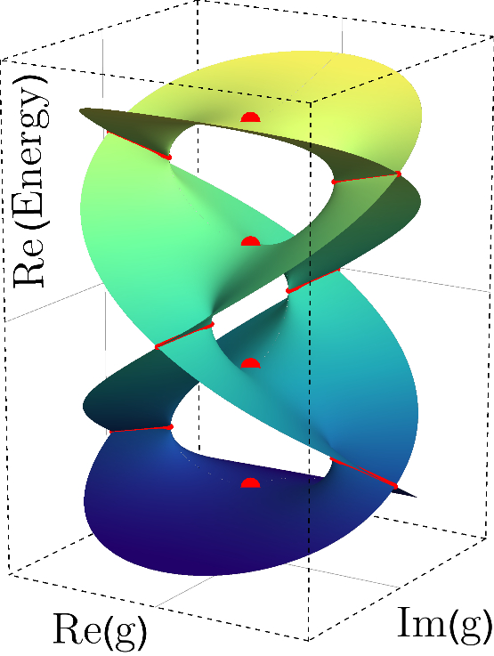
((a))

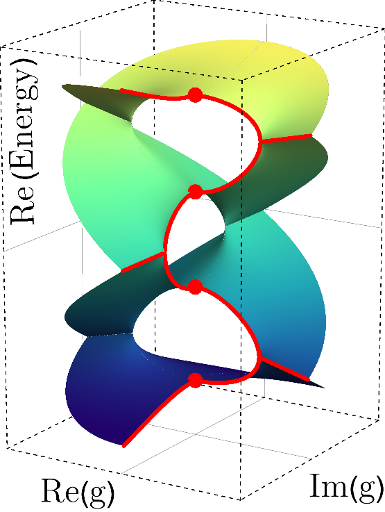
((b))

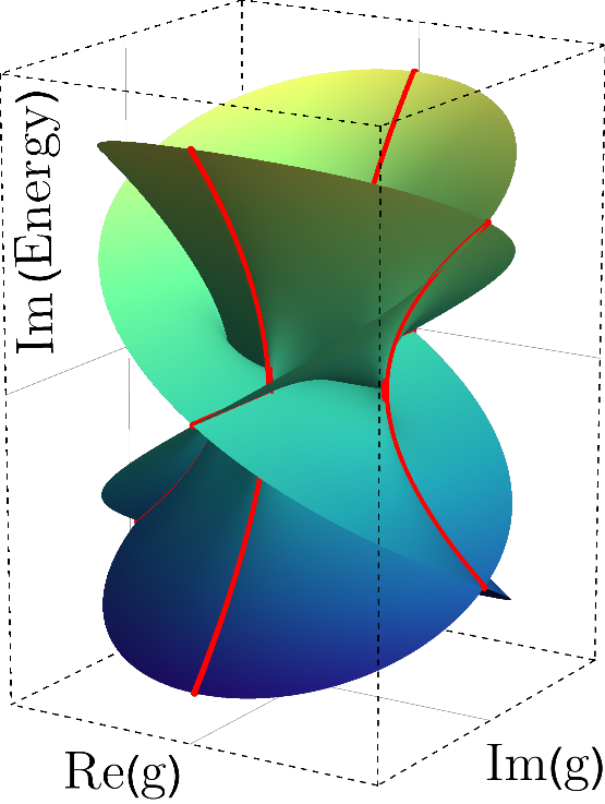
((c))

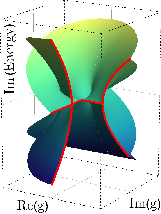
((d))

Figure 1: Riemann surface structure of the ground-state energy function $E_{0}(g)$ over the complex coupling plane for $\nu>\omega$. Figures (a) and (b) show the real part of the Riemann surface. The red dots denote the four (purely real) decoupling limits $E_{0}(0)=\pm(\nu\pm\omega)$. In Fig. (a) the branch cuts are denoted as solid red lines, while in Fig. (b) the fourth quadrant of the coupling plane is cut out and the characteristics of the energy function at the cuts along the real and imaginary coupling axes are denoted as solid red lines. Figures (c) and (d) display this visualisation for the imaginary part of $E_{0}(g)$.

In CHO (7) it was shown that with the ansatz

$$\psi_{0}=a_{0,0}\cdot\mathrm{e}^{-\alpha x^{2}/2-\beta y^{2}/2+\gamma xy}$$ (2)

for the ground-state wave function, where the parameters $\alpha$, $\beta$ and $\gamma$ are to be determined and $a_{0,0}$ is an overall normalisation constant, Schrödinger’s eigenvalue equation $H\psi=E\psi$ for $H$ as given in (1) leads to the system of equations

$$E_{0} =\alpha+\beta$$ (3)

$$g\, =-2(\alpha+\beta)\gamma$$ (4)

$$\nu^{2} =\alpha^{2}+\gamma^{2}$$ (5)

$$\omega^{2} =\beta^{2}+\gamma^{2}\,,$$ (6)

which describes the energy eigenvalues $E_{0}$ of the ground state and relates the parameters $\alpha$, $\beta$ and $\gamma$ to the natural oscillator frequencies and the complex coupling constant $g$. Eliminating these parameters in the energy equation (3) leads to the quartic polynomial energy equation

$$E_{0}^{4}-2(\nu^{2}+\omega^{2})E_{0}^{2}+(\nu^{2}-\omega^{2})^{2}+g^{2}=0$$ (7)

that is solved by the ground-state energy function

$$E_{0}(g)=\pm\sqrt{\nu^{2}+\omega^{2}\pm\sqrt{4\nu^{2}\omega^{2}-g^{2}}}\,.$$ (8)

This nested square-root function describes a four-fold dependence of the energy on the complex coupling constant $g$. It has six (square-root type) branch points, four occurring at the coupling values $g=\pm 2\nu\omega$ and two at $g=\pm i\,(\nu^{2}-\omega^{2})$ and the associated branch cuts allow the transition between the four sheets of the Riemann surface of $E_{0}(g)$ through a variation of the coupling constant in the complex plane. It was noted in particular that the possible ground states of the decoupled theory $E_{0}(0)=\pm\nu\pm\omega$ correspond to the four possible combinations of the conventional and unconventional phases of the ground states of the two constituent oscillators and that the continuation in the coupling $g$ thus allows for a smooth transition between the states in this quartet structure. This result implies that one can in principle extract energy from the conventional ground state of the system. However, work must be done in moving $g$ in the complex plane to go from one sheet to another. One notes that for $g=0$ all possible values of $E_{0}(g)$ are purely real, a fact which can be traced back to the ${\mathcal{PT}}$ symmetry of the Hamiltonian for real values of $g$. In Figs. 1(a) and 1(c) we have visualized the four-fold Riemann structure associated with this result. The red dots on these plots indicate the decoupling limit where $g=0$, while the branch cuts are shown as solid red lines. In Figs. 1(b) and 1(d) we have in addition cut out the fourth quadrant and indicated with a further solid red line a possible path that can be taken to move from one decoupling limit at $g=0$ to another in a continuous fashion.

II.2 First excited state

In order to show that the quartet connection structure found for the ground state is repeated for higher excitation states of the system, one can investigate the structure of the decoupled theory for the first excited state of the system. The goal is to show that the energy eigenvalues of the decoupled theory of the system can generally be collected in sets that contain four possible combinations of spectral phases of the excitation states of the constituent oscillators and that these four eigenvalues are analytic continuations of each other in the complex coupling plane. In CHO (7), the ad-hoc ansatz for the wave function

$$\psi=[a_{1,0}x+a_{0,1}y+a_{1,1}xy+a_{0,0}]\cdot\mathrm{e}^{-\alpha x^{2}/2-\beta y^{2}/2+\gamma xy}$$ (9)

was inserted into the eigenvalue equation and the resulting system of equations was analysed: it was found that the eigenvalues of the decoupled theory with $g=0$ can indeed be collected in such quartets. In the following we show, however, that already at this stage with the first excited state of the system, the analytic connection of the states is not restricted to these quartets and shows a more intricate structure.

In the discussion of the ground state the exponential wave function ansatz (2) was chosen, as it is the most general function without roots that can satisfy the boundary conditions of an asymptotically vanishing wave function and balance the eigenvalue equation in the limit of large position variables $x$ and $y$. For higher excitation states $\psi_{n}(x,y)$ the asymptotically dominating exponential behaviour remains, but instead of being multiplied with the single (normalising) overall constant $a_{0,0}$ as in (2), we now include a polynomial prefactor $P_{n}(x,y)$ of $n$th degree to take into account the $n$ roots of the eigenfunction that we expect for the $n$th excited state of the system, in analogy to Courant’s nodal line theorem that holds in the single position variable case:

$$\psi_{n}(x,y)=P_{n}(x,y)\cdot\mathrm{e}^{-\alpha x^{2}/2-\beta y^{2}/2+\gamma xy}\,,$$ (10)

where

$$P_{n}(x,y)=\sum_{i=0}^{n}\sum_{j=0}^{i}a_{i,i-j}x^{i}y^{i-j}\,.$$ (11)

For the first excited state this ansatz takes the form

$$\psi_{1}(x,y)=[a_{1,0}x+a_{0,1}y+a_{0,0}]\cdot\mathrm{e}^{-\alpha x^{2}/2-\beta y^{2}/2+\gamma xy}$$ (12)

Substituting it into Schrödinger’s eigenvalue equation leads to the following system of equations

$$0 =a_{0,0}\,(E_{1}-\alpha\,-\beta)$$ (13)

$$0 =a_{0,0}\,(2(\alpha\,+\beta)\gamma+g)$$ (14)

$$0 =a_{0,0}\,(\alpha^{2}+\gamma^{2}-\nu^{2})$$ (15)

$$0 =a_{0,0}\,(\beta^{2}+\gamma^{2}-\omega^{2})$$ (16)

$$0 =a_{1,0}\,(E_{1}-3\alpha\,-\beta)+a_{0,1}\,(2\gamma)$$ (17)

$$0 =a_{0,1}\,(E_{1}-\alpha\,-3\beta)+a_{1,0}\,(2\gamma)$$ (18)

$$0 =a_{1,0}\,(\alpha^{2}+\gamma^{2}-\nu^{2})-a_{0,1}\,(2(\alpha\,+\beta)\gamma+g)$$ (19)

$$0 =a_{0,1}\,(\beta^{2}+\gamma^{2}-\omega^{2})-a_{1,0}\,(2(\alpha\,+\beta)\gamma+g)$$ (20)

$$0 =a_{0,1}\,(\alpha^{2}+\gamma^{2}-\nu^{2})$$ (21)

$$0 =a_{1,0}\,(\beta^{2}+\gamma^{2}-\omega^{2})\,.$$ (22)

We recognise the equations (13) to (16) as being the ground-state system of equations (3) to (6) with the difference that the coefficient $a_{0,0}$ may vanish this time. However, if $a_{0,0}$ does not vanish the equations (4) to (6) and (14) to (16) coincide, and the energy equations (3) and (13) imply that $E_{1}=E_{0}$. For the calculation of the general energy function $E_{1}(g)$ we can thus focus on the system of remaining equations (17) to (22). This system again contains one part that describes the energy eigenvalues of the system and one that relates the parameters $\alpha$, $\beta$ and $\gamma$ to the natural oscillator frequencies $\nu$ and $\omega$ and the coupling constant $g$. The two coupled energy equations (17) and (18) can be combined to yield the quadratic energy equation

$$E_{1}^{2}-4(\alpha+\beta)E_{1}+3(\alpha+\beta)^{2}+4(\alpha\beta-\gamma^{2})=0$$ (23)

and the equations (19) to (22) are equivalent to the equations (4) to (6) found in the ground-state system, because at least one of the coefficients $a_{0,1}$ and $a_{1,0}$ must not vanish in order for $P_{1}(x,y)$ to be a first degree polynomial. To eliminate the parameters $\alpha$, $\beta$ and $\gamma$ in terms of the parameters of the Hamiltonian $\nu$, $\omega$ and $g$ we use the definition of the ground-state energy (3) and the relations (4) to (6) to rewrite equation (23) as

$$E_{1}^{2}-4E_{0}\cdot E_{1}+\Bigl{(}3E_{0}^{2}\pm 2\cdot\sqrt{4\nu^{2}\omega^{2}-g^{2}}\Bigr{)}=0\,,$$ (24)

where the $\pm$ sign coincides with the choice of sign for the inner square root in $E_{0}(g)$. Now making use of the ground-state energy result (8), we can express the solutions to (24) as

$$\begin{split}E_{1}^{+}(g)=\pm 2&\sqrt{\nu^{2}+\omega^{2}+\sqrt{4\nu^{2}\omega^{2}-g^{2}}}\\ \pm&\sqrt{\nu^{2}+\omega^{2}-\sqrt{4\nu^{2}\omega^{2}-g^{2}}}\vspace{-.3cm}\end{split}$$ (25)

and

$$\begin{split}E_{1}^{-}(g)=\pm 2&\sqrt{\nu^{2}+\omega^{2}-\sqrt{4\nu^{2}\omega^{2}-g^{2}}}\\ \pm&\sqrt{\nu^{2}+\omega^{2}+\sqrt{4\nu^{2}\omega^{2}-g^{2}}}\,,\end{split}$$ (26)

taking care to choose the appropriate signs of the inner square root of $E_{0}(g)$. The possibilities $E_{1}^{+}(g)$ and $E_{1}^{-}(g)$, in which the inner square root of the first term in the solution is evaluated with a positive or negative sign respectively, are thus denoted separately.

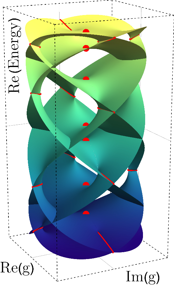
((a))

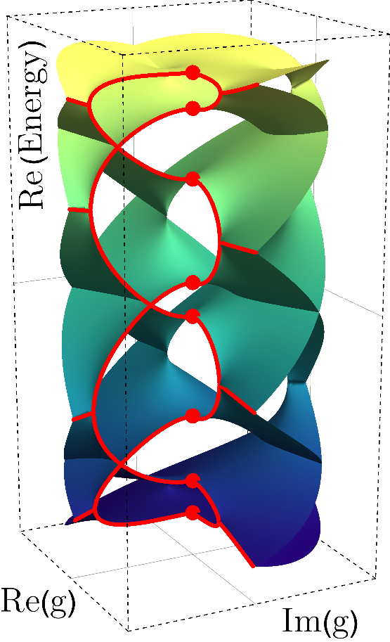
((b))

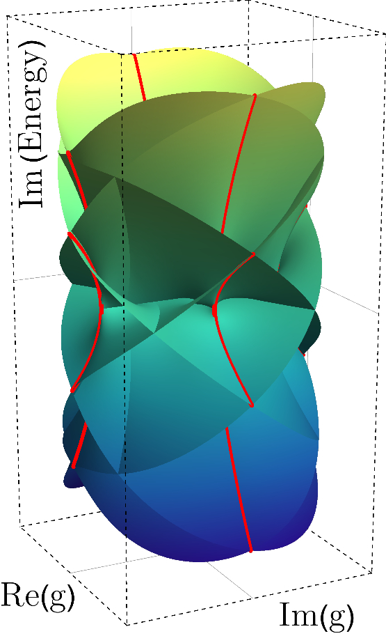
((c))

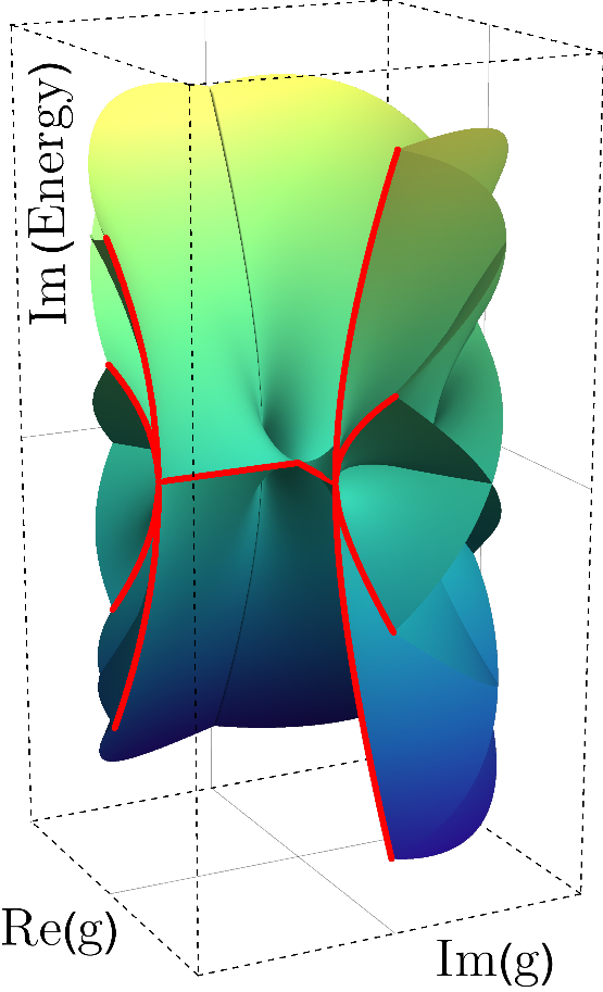
((d))

Figure 2: Riemann surface structure of the first excited state energy function $E_{1}(g)$ over the complex coupling plane for $\nu>3\omega$. Figures (a) and (b) show the real part of the Riemann surface. The red dots denote the eight (purely real) decoupling limits $\pm(3\nu\pm\omega)$ and $\pm(\nu\pm 3\omega)$. In Fig. (a) the branch cuts are denoted as solid red lines, while in Fig. (b) the fourth quadrant of the coupling plane is cut out and the characteristics of the energy function at the cuts along the real and imaginary coupling axes are denoted as solid red lines. Figures (c) and (d) display this visualisation for the imaginary part of $E_{1}(g)$.

The eigenvalues of the decoupled theory of the first excited state can then be seen to be

$$E_{1}^{+}(0)=\pm 2(\nu+\omega)\pm(\nu-\omega)\vspace{-.3cm}$$ (27)

and

$$E_{1}^{-}(0)=\pm 2(\nu-\omega)\pm(\nu+\omega)\,.$$ (28)

These eight solutions can in fact be collected into two sets of four solutions: $\pm 3\nu\pm\omega$ and $\pm\nu\pm 3\omega$, which show a similar quartet structure to that found for the ground state of the system, recovering the result of CHO (7). Each set contains the four possible combinations of conventional and unconventional phases of one constituent oscillator being in its first excited state and one being in its ground state. Although there is a resemblance to the analytic structure of the ground state, the general connection structure has changed: Instead of finding two separate quartets of analytically connected energies of the decoupled theory we find one single energy function $E_{1}(g)$ with sixteen (square-root type) branch points - eight at $g=\pm 2\nu\omega$ and eight at $g=\pm i\,(\nu^{2}-\omega^{2})$ - with associated branch cuts that connect eight sheets of the Riemann surface of this energy function pairwise to one another. A visualisation of this surface is shown in Figs. 2(a) to 2(d).

The Riemann surface of the first excited state of the system thus describes an analytic connection of decoupled states in an octet rather than in a quartet. This octet contains the two quartets - each describing the four possible combinations of the conventional and unconventional spectral phases of the two constituent oscillators of the decoupled theory being in excited states whose respective quantum numbers add up to the total quantum number $n$ describing the excited state of the complete system - which are mirror images of each other under the exchange of the constituent oscillators in the decoupled theory.

Furthermore, we can understand the four-fold structure of the ground state as a special case of this octet structure, in which the two quartets contained in the octet of decoupled states are identical because both constituent oscillators of the decoupled system are in the same excited state (namely the ground state).

II.3 General excited states

The analysis of the first excited state led us to the conclusion that the quartet structure of the energy levels that we found for the ground state of the system does not mean that the Riemann surfaces are four-fold for higher excited states. In particular, we found an octet structure for the first excited state that included the quartet structure as a special case ($g=0$). In this section we show that this octet structure of analytically connected energy levels of the decoupled system is in fact the fundamental structure of the system in the sense that it is repeated for higher excitations.

Inserting the general wave function ansatz

$$\psi_{n}(x,y)=P_{n}(x,y)\cdot\mathrm{e}^{-\alpha x^{2}/2-\beta y^{2}/2+\gamma xy}\,,$$ (29)

into the eigenvalue equation and comparing coefficients in $x$ and $y$ leads to the set of equations

$$(M_{n})_{j,i-j}=0\,,$$ (30)

where $i\in\{0,...,n+2\}$, $j\in\{0,...,i\}$ and $(M_{n})_{j,i-j}$ is given as

$$\begin{split}(M_{n})_{j,i-j}=\quad&\bigl{[}E_{n}-\alpha(2j+1)-\beta(2(i-j)+1)\bigr{]}\,a_{j,i-j}\\ +&\bigl{[}-(2(\alpha+\beta)\gamma+g)\bigr{]}\,a_{j-1,i-j-1}\\ +&\bigl{[}\alpha^{2}+\gamma^{2}-\nu^{2}\bigr{]}\,a_{j-2,i-j}\\ +&\bigl{[}\beta^{2}+\gamma^{2}-\omega^{2}\bigr{]}\,a_{j,i-j-2}\\ +&\bigl{[}(2\gamma)\cdot(j+1)\bigr{]}\,a_{j+1,i-j-1}\\ +&\bigl{[}(2\gamma)\cdot(i-j+1)\bigr{]}\,a_{j-1,i-j+1}\\ +&\bigl{[}(j+2)(j+1)\bigr{]}\,a_{j+2,i-j}\\ +&\bigl{[}(i-j+2)(i-j+1)\bigr{]}\,a_{j,i-j+2}\,.\end{split}$$ (31)

The polynomial factor $P_{n}(x,y)$ in the ansatz (29) is a polynomial of $n$th degree, such that at least one of the coefficients $a_{j,n-j}$ must not vanish. In particular, there exists one such coefficient with largest index $j$, such that $\forall k\in\{0,...,n\}$ with $k>j$ it follows that $a_{k,n-k}=0$. Using the equations $(M_{n})_{j+2,n-j}=0$, $(M_{n})_{j+1,n-j+1}=0$ and $(M_{n})_{j,n-j+2}=0$, we conclude that the equations (4) to (6), which relate the parameters $\alpha$, $\beta$ and $\gamma$ that determine the asymptotically dominating exponential behaviour of the eigenfunctions to the natural oscillator frequencies $\nu$ and $\omega$ and the coupling constant $g$, are generally satisfied for all excitations of the system. Furthermore, this simplifies the expression (31) such that the system of equations becomes a system of $(n+1)(n+2)/2$ coupled energy equations. The equations (30) with $i=n$ form a subsystem which, after making the substitution $\lambda_{k}=\bigl{[}E_{n}-\alpha(2k+1)-\beta(2(n-k)+1)\bigr{]}$, takes the plain form

$$\bigl{[}M_{n}\bigr{]}_{0,n}:\quad \lambda_{0}\,a_{0,n} =\,\, 1\cdot(-2\gamma)\,a_{1,n-1}$$ (32)

$$\bigl{[}M_{n}\bigr{]}_{1,n-1}:\quad \lambda_{1}\,a_{1,n-1} =\,\, 2\cdot(-2\gamma)\,a_{2,n-2}$$

$$\,\,\,+ n\cdot(-2\gamma)\,a_{0,n}$$

$$\bigl{[}M_{n}\bigr{]}_{2,n-2}:\quad \lambda_{2}\,a_{2,n-2} =\,\, 3\cdot(-2\gamma)\,a_{3,n-3}$$

$$\,\,\,+ (n-1)\cdot(-2\gamma)\,a_{1,n-1}$$

$$\hskip 7.11317pt...$$

$$\bigl{[}M_{n}\bigr{]}_{n-1,1}:\quad \lambda_{n-1}\,a_{n-1,1} =\,\, n\cdot(-2\gamma)\,a_{n,0}$$

$$\,\,\,+ 2\cdot(-2\gamma)\,a_{n-2,2}$$

$$\bigl{[}M_{n}\bigr{]}_{n,0}:\quad \lambda_{n}\,a_{n,0} =\,\, 1\cdot(-2\gamma)\,a_{n-1,1}.$$

Solving this subsystem of equations leads to an expression for the energy eigenvalues: we combine the equations in (32) by eliminating the coefficients $a_{l,n-l}$ to obtain a general polynomial energy equation for the $n$th excited state:

$$\prod_{i=0}^{n}\lambda_{i}= -\sum_{r=1}^{\left\lfloor(n+1)/2\right\rfloor}\biggl{(}\,\prod_{i=0}^{n}\lambda_{i}\biggr{)}\cdot$$

$$\prod_{m=1}^{r}\,\biggl{(}\,\sum_{k_{m}=k_{m-1}+2}^{(n+1)-2(r+1-m)}-\,\frac{(n-k_{m})(k_{m}+1)(-2\gamma)^{2}}{\lambda_{k_{m}}\,\lambda_{k_{m}+1}}\biggr{)}\,.$$

For the first five excited states this equation reads explicitly:

$$(n=0):\quad E_{0}-(\alpha+\beta)=0$$

$$(n=1):\quad E_{1}^{2}-4E_{1}\cdot(\alpha+\beta)+$$

$$\Bigl{(}4(\alpha+\beta)^{2}-((\alpha-\beta)^{2}+4\gamma^{2})\Bigr{)}=0$$

$$(n=2):\quad E_{2}^{3}-9E_{2}^{2}\cdot(\alpha+\beta)+$$

$$E_{2}\Bigl{(}27(\alpha+\beta)^{2}-4((\alpha-\beta)^{2}+4\gamma^{2})\Bigr{)}-$$

$$\Bigl{(}27(\alpha+\beta)^{3}-12(\alpha+\beta)((\alpha-\beta)^{2}+4\gamma^{2})\Bigr{)}$$

$$=0$$

$$(n=3):\quad E_{3}^{4}-16E_{3}^{3}\cdot(\alpha+\beta)+$$

$$E_{3}^{2}\cdot\Bigl{(}96(\alpha+\beta)^{2}-10((\alpha-\beta)^{2}+4\gamma^{2})\Bigr{)}-$$

$$E_{3}\cdot\Bigl{(}256(\alpha+\beta)^{3}-$$

$$80(\alpha+\beta)((\alpha-\beta)^{2}+4\gamma^{2})\Bigr{)}+$$

$$\Bigl{(}256(\alpha+\beta)^{4}-160(\alpha+\beta)^{2}((\alpha-\beta)^{2}+4\gamma^{2})+$$

$$9((\alpha-\beta)^{2}+4\gamma^{2})^{2}\Bigr{)}=0$$

$$(n=4):\quad E_{4}^{5}-25E_{4}^{4}\cdot(\alpha+\beta)+E_{4}^{3}\cdot\Bigl{(}250(\alpha+\beta)^{2}-$$

$$20((\alpha-\beta)^{2}+4\gamma^{2})\Bigr{)}-$$

$$E_{4}^{2}\cdot\Bigl{(}1250(\alpha+\beta)^{3}-$$

$$300(\alpha+\beta)((\alpha-\beta)^{2}+4\gamma^{2})\Bigr{)}+$$

$$E_{4}\cdot\Bigl{(}3125(\alpha+\beta)^{4}-$$

$$1500(\alpha+\beta)^{2}((\alpha-\beta)^{2}+4\gamma^{2})+$$

$$64((\alpha-\beta)^{2}+4\gamma^{2})^{2}\Bigr{)}-$$

$$\Bigl{(}3125(\alpha+\beta)^{5}-$$

$$2500(\alpha+\beta)^{3}((\alpha-\beta)^{2}+4\gamma^{2})+$$

$$320(\alpha+\beta)((\alpha-\beta)^{2}+4\gamma^{2})^{2}\Bigr{)}=0$$

and is solved by the following energy functions

$$(n=0):\,\, E_{0}=1\cdot(\alpha\,+\beta)\,,$$ (33)

$$(n=1):\,\, E_{1}=2\cdot(\alpha\,+\beta)\pm 1\cdot\sqrt{(\alpha\,-\beta)^{2}+4\gamma^{2}}\,,$$ (34)

$$(n=2):\,\, E_{2}=3\cdot(\alpha\,+\beta)\,,$$ (35)

$$E_{2}=3\cdot(\alpha\,+\beta)\pm 2\cdot\sqrt{(\alpha\,-\beta)^{2}+4\gamma^{2}}\,,$$ (36)

$$(n=3):\,\, E_{3}=4\cdot(\alpha\,+\beta)\pm 1\cdot\sqrt{(\alpha\,-\beta)^{2}+4\gamma^{2}}\,,$$ (37)

$$E_{3}=4\cdot(\alpha\,+\beta)\pm 3\cdot\sqrt{(\alpha\,-\beta)^{2}+4\gamma^{2}}\,,$$ (38)

$$(n=4):\,\, E_{4}=5\cdot(\alpha\,+\beta)\,,$$ (39)

$$E_{4}=5\cdot(\alpha\,+\beta)\pm 2\cdot\sqrt{(\alpha\,-\beta)^{2}+4\gamma^{2}}\,,$$ (40)

$$E_{4}=5\cdot(\alpha\,+\beta)\pm 4\cdot\sqrt{(\alpha\,-\beta)^{2}+4\gamma^{2}}\,.$$ (41)

This is in particular in agreement with the results for the ground state (see Eq. (3)) and the first excited state (see Eq. (23)). We thus find that the energy function solutions take the form

$$E_{n}=(n+1)\cdot(\alpha\,+\beta)\pm m\cdot\sqrt{(\alpha\,+\beta)^{2}-4(\alpha\beta-\gamma^{2})}$$ (42)

with $m$ running through all even natural numbers up to $n$ for even excitations $n$, i.e. $m\in\{0\}\cup\{x\mid x\in\mathbb{N}\,\land\,(x\mid 2)\,\land\,(x\leq n)\}$, and $m$ running through all odd natural numbers up to $n$ for odd $n$, i.e. $m\in\{x\mid x\in\mathbb{N}\,\land\,(x\nmid 2)\,\land\,(x\leq n)\}$. As in the discussion of the first excited state, this can be rewritten using the result for the ground-state energy as

$$\begin{split}E_{n}^{+}(g)=\pm(n+1)\cdot&\sqrt{\nu^{2}+\omega^{2}+\sqrt{4\nu^{2}\omega^{2}-g^{2}}}\,\\ \pm m\cdot&\sqrt{\nu^{2}+\omega^{2}-\sqrt{4\nu^{2}\omega^{2}-g^{2}}}\vspace{-.1cm}\end{split}$$ (43)

and

$$\begin{split}E_{n}^{-}(g)=\pm(n+1)\cdot&\sqrt{\nu^{2}+\omega^{2}-\sqrt{4\nu^{2}\omega^{2}-g^{2}}}\,\\ \pm m\cdot&\sqrt{\nu^{2}+\omega^{2}+\sqrt{4\nu^{2}\omega^{2}-g^{2}}}\,.\end{split}$$ (44)

We have again expressed the single energy function $E_{n}(g)$ in terms of two solutions $E_{n}^{+}(g)$ and $E_{n}^{-}(g)$, in order to emphasize the possible sign choices of the nested square-root functions.

The solutions in (43) and (44) for arbitrary $n$ strongly resemble the energy function of the first excited state. And although they differ in the scaling factors of the two nested square-root functions, the eight-fold structure of the energy function solutions remains. The eigenvalues of the decoupled theory can now be collected into two quartets $\pm(n+1+m)\,\nu\pm(n+1-m)\,\omega$ and $\pm(n+1-m)\,\nu\pm(n+1+m)\,\omega$ which are mirror images of each other under an exchange of the constituent oscillators of the decoupled theory; an analytic continuation of the coupling constant $g$ allows for a smooth transition between these eight states. Note as well that as $m$ runs through all non-negative even or odd numbers up to $n$ the coefficients of $\nu$ and $\omega$ in the two quartets run through the odd natural numbers up to $2n+1$ in such a way that the sum of the (absolute values of the) coefficients is $2(n+1)$, reflecting that for each possible value of $m$ the sum of the quantum numbers of the constituent oscillators in the decoupled theory is the quantum number $n$ of the complete system, as expected If $m=0$ (see eg. (33), (35) and (39)) we find four-fold energy functions which can be understood as special cases of the general octet structure in the way described in the last section: the two quartets, which are collected in an octet of decoupled states and which are mirror images of each other under an exchange of the constituent oscillators of the decoupled theory, are identical, because both constituent oscillators of the decoupled system are in the same excited state, i.e. the state with quantum number $n/2$. The generally eight-sheeted Riemann surface of the energy function in (43) and (44) simplifies to a four-fold structure (as that found in the discussion of the ground state of the system) accordingly, because the sheets coincide pairwise.

In contrast to the solutions that we found for the ground state and first excited state the solution for higher excited states cannot be written simply as a single analytic function. The constant $m$ may take $\left\lfloor(n+1)/2\right\rfloor$ different values at the $n$th excitation of the system. This means that although sets (quartets or octets) of energy eigenvalues of the decoupled theory at this excitation level are analytic continuations of each other, different sets remain separated. These different sets and their associated Riemann surface can be characterised by the quantum number $n$ describing the excitation state of the complete system and the number $m$ describing the difference of the excited states of the constituent oscillators in the decoupled theory. We emphasise, in agreement with CHO (7), that energy levels of different excited states of the complete system, i.e. belonging to sets with different values of $n$, are not analytically connected.

The energy functions in (43) and (44) can furthermore be confirmed using canonical transformations of the Hamiltonian trafo (8) to decouple the system into the form

$$H^{\prime}=p^{\prime\,2}+\Omega_{+}^{2}\,x^{\prime\,2}+q^{\prime\,2}+\Omega_{-}^{2}\,y^{\prime\,2}\,.$$

with the effective oscillator frequencies

$$\Omega_{\pm}=\sqrt{\frac{(\nu^{2}+\omega^{2})\pm\sqrt{g^{2}+(\nu^{2}-\omega^{2})^{2}}}{2}}\,.$$

We note in particular that the wave functions resulting from this decoupled effective oscillator description satisfy the relations (4) to (6) such that the boundary value structure of the transformed problem does indeed agree with the structure of the original system that we approached using a wave function ansatz motivated by an asymptotic analysis. The transformational approach to solving the eigenvalue equation will, however, fail at the branch points of the energy function, because either the effective frequencies vanish or the condition for the canonicity of the transformation is not satisfied.

III The structure of the analytic connection

The connection of all four possible spectral phases of the two constituent oscillators of the decoupled theory through an analytic continuation in the coupling constant $g$ is one of the principle results of CHO (7). We showed that the four-fold connection structure of the energy that is found for the ground state does not repeat itself in all excited states of the complete system, as was originally suspected in CHO (7), but should instead be understood as a special case of an eight-fold structure that connects decoupled states, which are mirror images under an exchange of the constituent oscillators. However, the result of an analytic connection between different spectral phases of the decoupled theory is retained.

III.1 Spectral phases of the harmonic oscillator

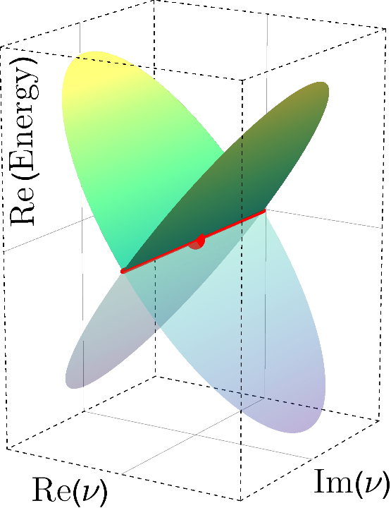
((a))

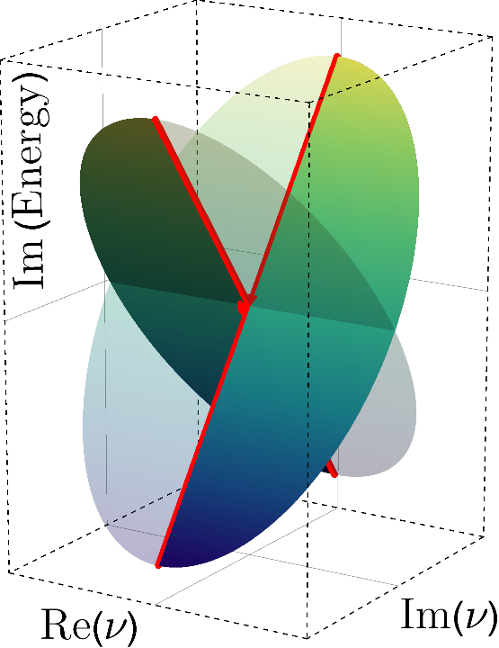
((b))

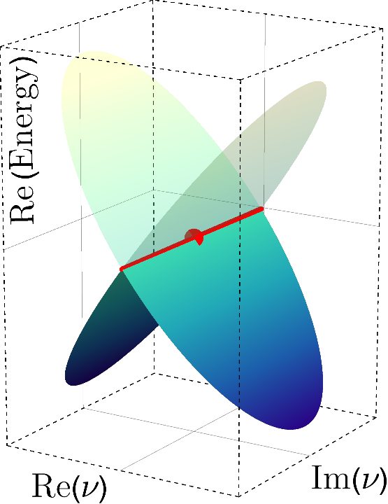
((c))

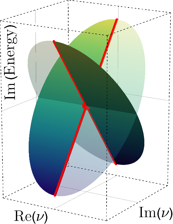
((d))

Figure 3: Riemann surface structure of the ground-state energy function $E_{0}(\nu)=\pm\sqrt{\nu^{2}}$ in the complex frequency plane. Figures (a) and (b) show the real and imaginary parts of the Riemann surface on the first sheet respectively. Figures (c) and (d) show the real and imaginary parts on the second sheet. The dot in the center denotes the point $E_{0}(\nu=0)=0$, at which the two sheets coincide. This point can be characterised as two coalescing square-root branch points. The associated branch cuts are drawn as solid red lines along the imaginary frequency axis in the chosen representation.

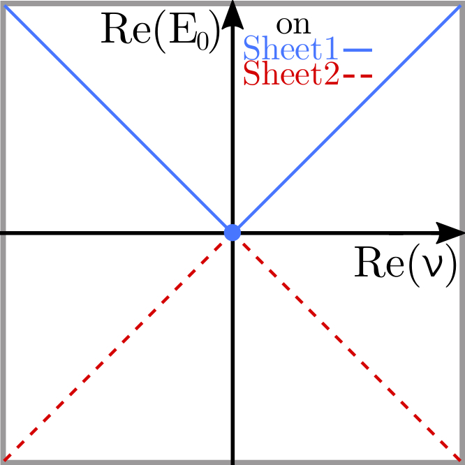
((a))

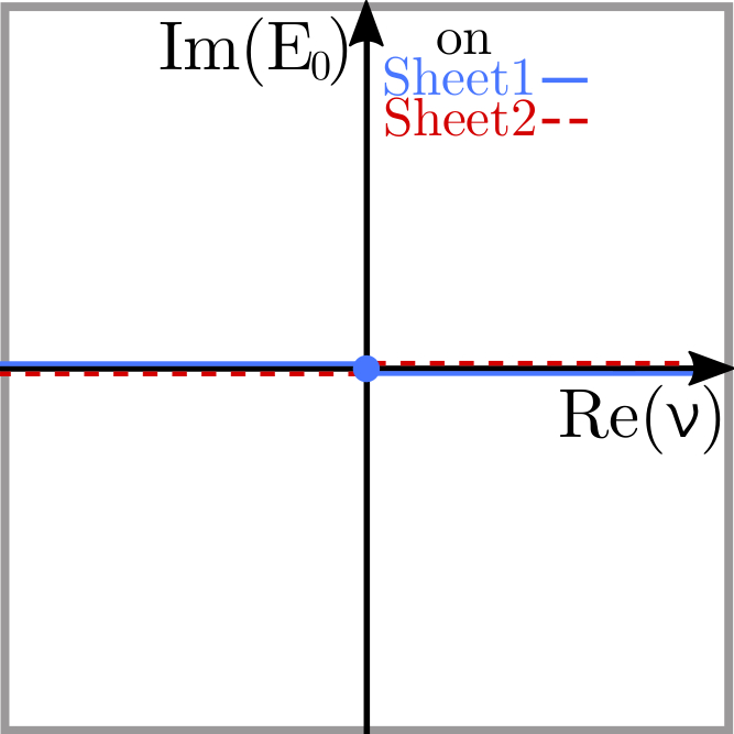
((b))

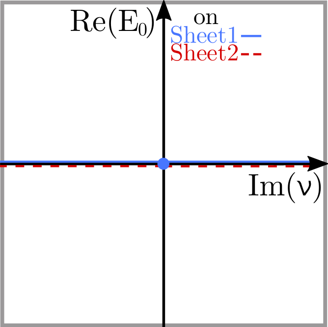
((c))

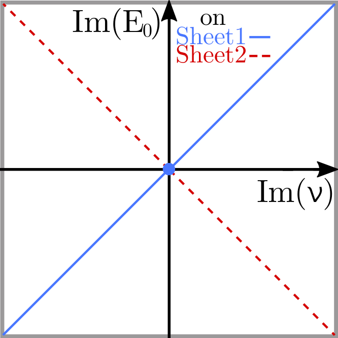
((d))

Figure 4: Behaviour of the real and imaginary parts of the harmonic oscillator ground state energy function $E_{0}(\nu)$ along the real and imaginary frequency axis. The behaviour on the first sheet is denoted by the solid blue line and on the second sheet by the dashed red one. The blue dot in the center of each graph denotes the coalescing square-root branch points at vanishing frequency.

The occurrence of different spectral phases and their connection through an analytic continuation is in itself not surprising. A conventional and an unconventional spectrum can, for example, be found for the single harmonic oscillator, $H=p^{2}+\nu^{2}z^{2}$, where a connection between both is established by the analytic continuation of the natural oscillator frequency $\nu$ HO (9). Accordingly, we can find basic structural properties of the connection structure of the coupled oscillator system within the system of a single harmonic oscillator.

As argued in HO (9) the ground-state energy of the (complex) harmonic oscillator takes the form $E_{0}(\nu)=\pm\nu$, describing the conventional and the unconventional solutions. Notice that the eigenvalues of the two different spectral phases of the solution only agree for a vanishing frequency value. Although the energy function $E_{0}(\nu)$ can be calculated exactly in various ways, it is instructive to use a similar approach to the coupled oscillator system presented in Sec. II. Inserting the ansatz

$$\psi_{0}(z,\alpha)=c\cdot\mathrm{e}^{-\alpha z^{2}/2}$$ (45)

for the wave function into Schrödinger’s eigenvalue equation leads to the system of equations

$$E_{0} =\alpha$$

$$\nu^{2} =\alpha^{2}\,,$$

which we can easily solve for the energy and obtain the expression $E_{0}(\nu)=\pm\nu$. Nevertheless, the structure of the system of equations suggests that we should formulate the energy function as $E_{0}(\nu)=\pm\sqrt{\nu^{2}}$. A Riemann surface representation for general complex frequency values is displayed in Figs. 3(a) to 3(d). In the square-root notation $E_{0}(\nu)=\pm\sqrt{\nu}\cdot\sqrt{\nu}$ of the energy function we notice that the solution has two coalescing branch points at $\nu=0$. Furthermore, if we consider the behaviour of the energy eigenvalues as a function of purely real oscillator frequencies we find purely real eigenvalues that show a linear-crossing behaviour, which is similar to the behaviour of eigenvalues in the vicinity of a diabolic point. In contrast to a typical diabolic point, at which the two eigenfunctions associated with the coalescing eigenvalues remain linearly independent, the wave functions break down to the trivial solution in our case. Moreover, if we consider the behaviour of the energy as a function of purely imaginary frequencies, we find purely imaginary eigenvalues that show the same linear-crossing behaviour, see Figs. 4(a) to 4(d).

The behavior of the coalescing square-root branch points appears similar to that which occurs at a diabolic point. This, as well as the similarity to the structure of the coupled oscillator system, becomes more apparent if we consider the following modification of the harmonic oscillator Hamiltonian:

$$H^{+}=p^{2}+(\nu^{2}+\delta^{2})\,z^{2}\,,$$

with some small real positive constant $\delta$. For large frequencies this system resembles the common harmonic oscillator Hamiltonian. However, the wave function ansatz (45) leads to the ground-state energy function

$$E_{0}^{+}(\nu)=\alpha=\pm\sqrt{\nu^{2}+\delta^{2}}=\pm\sqrt{\nu-i\cdot\delta}\cdot\sqrt{\nu+i\cdot\delta}\,,$$

which reveals the distinct behaviour at small frequencies: this function has two separate branch points on the imaginary frequency axis at $\nu=\pm i\cdot\delta$. The associated Riemann surface is visualised in Figs. 5(a) to 5(d).

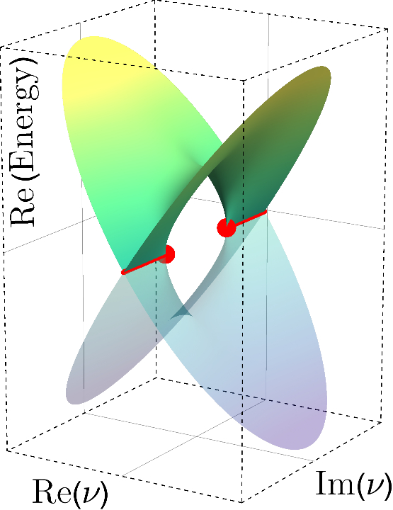
((a))

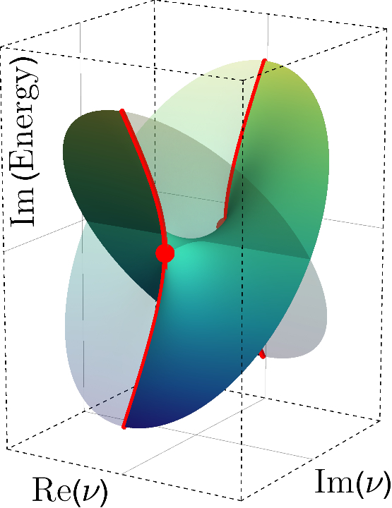
((b))

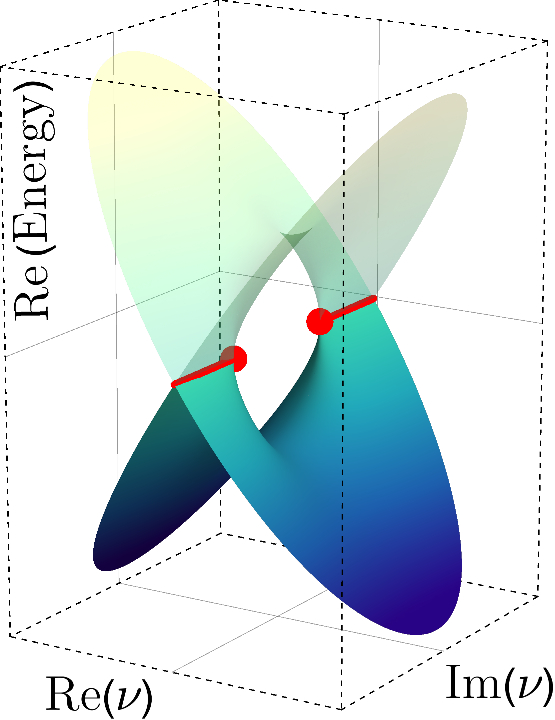
((c))

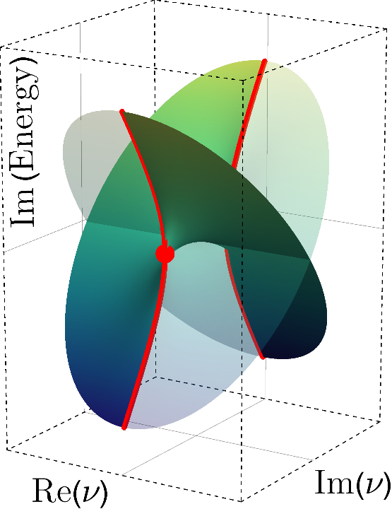
((d))

Figure 5: Riemann surface structure of the ground-state energy function $E_{0}^{+}(\nu)=\pm\sqrt{\nu-i\cdot\delta}\cdot\sqrt{\nu+i\cdot\delta}$ in the complex frequency plane. Figures (a) and (b) show the real and imaginary parts of the Riemann surface on the first sheet respectively, while Figs (c) and (d) show the real and imaginary parts on the second sheet. The dots denote the positions of the square-root branch points at $\nu=\pm i\cdot\delta$. The associated branch cuts are drawn as red lines along the imaginary frequency axis.

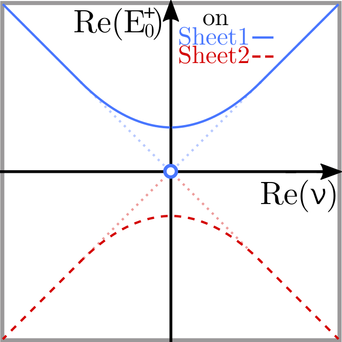
((a))

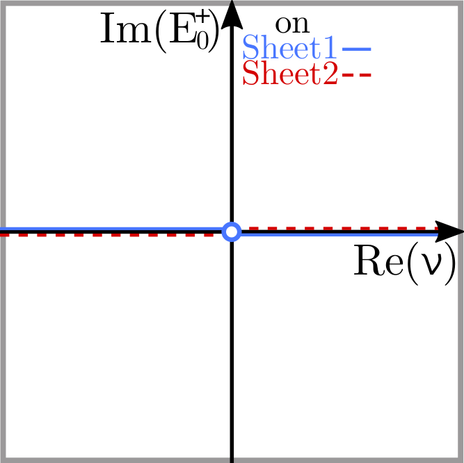
((b))

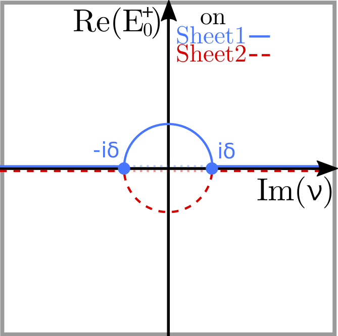
((c))

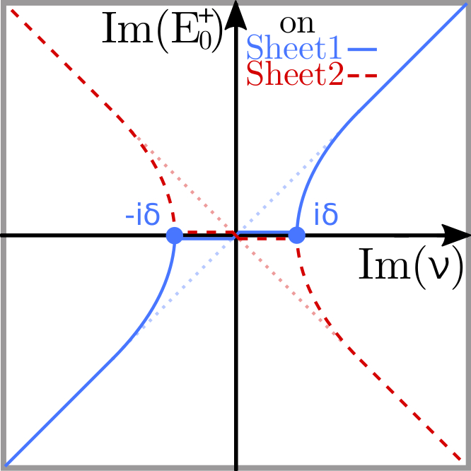
((d))

Figure 6: Behaviour of the real and imaginary parts of the modified harmonic oscillator ground-state energy function $E_{0}^{+}(\nu)$ along the real and imaginary frequency axis. The behaviour on the first sheet is denoted by the solid blue line and on the second sheet by the dashed red one. Solid blue dots denote the (imaginary) square-root branch points at $\nu=\pm i\cdot\delta$, while the open blue circle denotes the (vanishing) projection of these points onto the real frequency axis.

For frequency values along the real frequency axis we still find purely real energy eigenvalues. Notice, however, that the separation of the branch points along the imaginary frequency axis introduces an upper or lower bound $\pm\delta$ on the energy eigenvalues at real frequency values; the linear-crossing behaviour of the harmonic oscillator becomes an avoided-crossing behaviour, see Figs. 6(a) to 6(b). At the same time we notice that the eigenvalues associated with purely imaginary frequencies no longer take on only imaginary values. For imaginary frequencies with $\lvert\nu\rvert<\delta$ we obtain real energies instead, see Figs. 6(c) to 6(d). This behaviour has been referred to as re-entrant $\mathcal{PT}$ symmetry according to the symmetric nature of the Hamiltonian $H^{+}$ under parity-time reversal bubbles2 (10). That author notes a resemblance to ‘bubbles of instability’ in the equilibria of Hamiltonian systems, as described in bubbles (11). This resemblance is, however, superficial, as the bubble shown in Fig. 6 is associated with the existence of the two exceptional points. This differs from the result of bubbles (11), which requires a nonconservative or dissipative perturbation of the Hamiltonian to arrive at such a structure ONK (12, 13). Note that the avoided-crossing behaviour along the real frequency axis as well as the the behaviour along the imaginary axis can generally be found in the study of diabolic degeneracies. In diabolic (14) the eigenvalue surface near a diabolic point is unfolded due to a complex perturbation and the two possible structures found are the avoided crossing, which we encountered along the real frequency axis, and the so-called ‘double coffee filter’ behaviour. The latter is associated with the re-entrant symmetry and describes the behaviour along the imaginary frequency axis in our system, where the roles of the real and imaginary energy contributions are exchanged compared to the behaviour along the real frequency axis. Considering the (at least mathematical) connection of the two $\mathcal{PT}$-symmetric spectra of the modified oscillator potential that is represented in the Riemann surface in Fig. 5 we may think of the missing real eigenvalues at small frequencies along the real frequency axis as being shifted onto the imaginary frequency axis, where they introduce a region of unbroken $\mathcal{PT}$ symmetry to the spectrum that does not occur in the harmonic oscillator system $H$.

The formation of a diabolic point in the harmonic oscillator limit $\delta\rightarrow 0$ can be confirmed utilising the fact that the behaviour in the vicinity of the separated branch points is always equivalent to a two-dimensional problem, see chirality (15). For the system $H^{+}$ we find that the spectrum coincides globally with that of the matrix Hamiltonian

$$H^{\textrm{M}}=\begin{pmatrix}\delta&0\\ 0&-\delta\end{pmatrix}+\begin{pmatrix}0&\nu\\ \nu&0\end{pmatrix}\,.$$

The eigenfunctions associated with the eigenvalues $E^{\textrm{M}}_{\pm}$ are $\psi^{\mathrm{M}}_{+}=\big{(}\delta/\nu-\sqrt{1-(\delta/\nu)^{2}}\,,\,1\big{)}^{T}$ and $\psi^{\mathrm{M}}_{-}=\big{(}\delta/\nu+\sqrt{1-(\delta/\nu)^{2}}\,,\,1\big{)}^{T}$. If the frequency approaches the branch points $\nu\rightarrow\pm i\,\delta$, the eigenvectors of both sheets approach the same structure $\psi^{\mathrm{M}}_{+},\,\psi^{\mathrm{M}}_{-}\rightarrow(\mp i\,,\,1)^{T}$. This reflects the exceptional point nature of the square-root branch points. Furthermore, we can assign a definite left or right chirality to the branch points at $\nu=\pm i\,\delta$ depending on the structure of the eigenfunctions at those points, chirality (15), and notice that the two branch points have in any case opposite chiralities. On the other hand, if we consider the general eigenvector structure in the limit of coalescing branch points, i.e. when $\delta\rightarrow 0$, we find that the eigenvectors take the form $\psi^{\mathrm{M}}_{+}\rightarrow(-1\,,\,1)^{T}$ and $\psi^{\mathrm{M}}_{-}\rightarrow(+1\,,\,1)^{T}$. They are independent of the frequency and in particular remain linearly independent at the point $\nu=0$ at which the two branch points coalesce. Therefore the energy function of the harmonic oscillator system does indeed have a diabolic point at vanishing frequency $\nu$. This behaviour of two coalescing branch points with opposite chiralities forming a diabolic point has been described and measured by K. Ding et al. in a system with a four-state non-Hermitian Hamiltonian with coupling coalescence (16). The breakdown of the eigenfunctions $\psi_{0}(z)$ that we found in the study of the harmonic oscillator system is an independent phenomenon that occurs, because for vanishing frequencies the Hamiltonian $H$ takes the form of the free-particle Hamiltonian. The eigenfunctions should therefore take the form of plane waves. However, the boundary condition of vanishing wave functions imposed in the large position limit require these oscillating plane waves to vanish identically, causing the eigenfunction solution to break down.

III.2 The coupled system at equal frequencies

In this subsection we return to the analysis of the coupled harmonic oscillator system described by the Hamiltonian in (1), and view its structure in the light of the knowledge gained in Sec. IIIA. In the following we show that we can, in fact, find similar properties in the connection structure of the coupled system: a connection to $\mathcal{PT}$-symmetric cases of the system and the formation of diabolic points from coalescing branch points.

The decoupled theory of (1) describes a $\mathcal{PT}$-symmetric system with purely real eigenvalues, indicating an unbroken symmetry phase. The introduction of a purely real non-vanishing coupling constant $g$ preserves this symmetry and the energy eigenvalues remain real in a weakly coupled system. The unbroken symmetry phase for small coupling values does, however, break down when the coupling reaches the two (square-root) singularities of the general energy functions at $g=\pm 2\nu\omega$. For larger coupling values the eigenvalues become complex reflecting that the system is in a region of broken $\mathcal{PT}$ symmetry. The Hamiltonian (1) is, however, only $\mathcal{PT}$-symmetric in the special case of purely real coupling values and the analytic continuation in the coupling is foremost a mathematical tool to study the connection of the different spectral phases of the system. Nevertheless, real eigenvalues can not just be found in the unbroken symmetry region of real coupling values; we find them for purely imaginary couplings as well. At purely imaginary coupling values up to the general (square-root) singularities of the energy functions at $g=\pm i\,(\nu^{2}-\omega^{2})$ the eigenvalues are real and beyond these points they become complex. An exception is formed by energy levels belonging to quartet connection structures, where the energy remains real on the first and fourth sheet of the associated Riemann surface (corresponding to both constituent oscillators being in their conventional or both being in their unconventional phase in the decoupled limit) even beyond these points. This behaviour was first described in partial (17) and related to the partial $\mathcal{PT}$ symmetry of the Hamiltonian, in which parity reflection only acts on one of the two position variables $x$ and $y$. We thus find that the characteristic connection structure of energy levels through an analytic continuation in the coupling constant $g$ does not only enable the smooth transition between energy levels of different spectral phases, but that the square-root singularities of the energy functions, which essentially determine this structure, are related to the behaviour in the (partial) $\mathcal{PT}$-symmetric cases of the Hamiltonian as well. In these cases the the energy functions generally show an avoided-crossing behaviour along one coupling constant axis and an re-entrant behaviour along the other axis, similar to that found for the single harmonic oscillator.

Furthermore, the two imaginary branch points in the energy function of the coupled system at $g=\pm i\cdot(\nu^{2}-\omega^{2})$ coalesce in the limit of equal oscillator frequencies. The avoided-crossing behaviour becomes a linear-crossing behaviour of the energy levels (and the re-entrant bubble vanishes). At distinct natural oscillator frequencies $\nu$ and $\omega$ we can utilize the fact that the behaviour in the vicinity of the separated branch points is always equivalent to a two dimensional problem: we can assign a chirality to the branch points and find that the two imaginary branch points always have the opposite chirality. Thus two imaginary square-root branch points coalesce for the decoupled theory at $g=0$ and form a diabolic point similar to that found for the single harmonic oscillator. This also implies that the transformational approach fails for the decoupled theory. But the approach using a wave function ansatz based on asymptotic analysis is applicable and leads to the expected result, in which we simply take the equal frequency limit of the energy function solutions found earlier. There is, however, one special case: for vanishing coupling and equal oscillator frequencies $\nu=\omega$ the relations (4) to (6) imply that $\alpha=\beta=\pm\nu$ or $\alpha=-\beta=\pm\nu$.

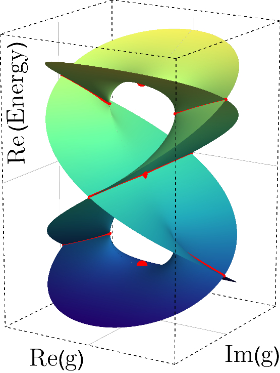
((a))

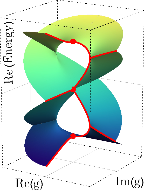
((b))

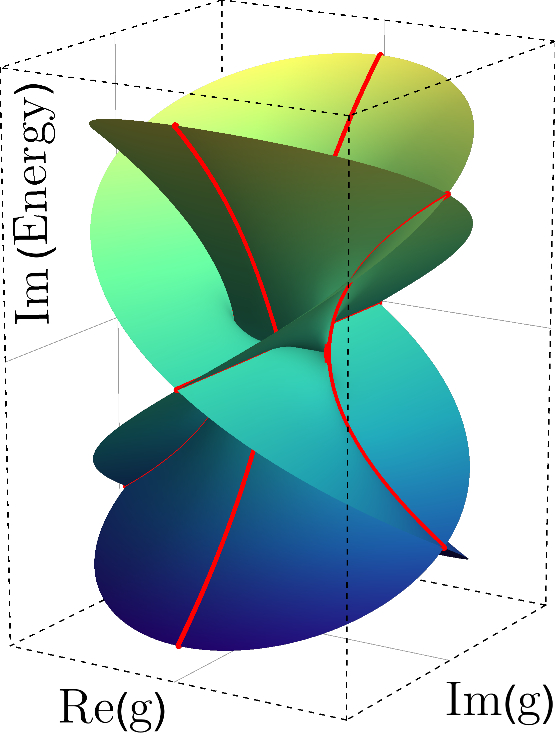
((c))

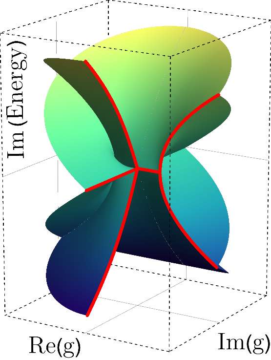
((d))

Figure 7: Riemann surface structure of the ground-state energy function $E_{0}(g)$ over the complex coupling plane for $\nu=\omega$. Figures (a) and (b) show the real part of the complete surface, while (c) and (d) display the imaginary part. Furthermore, in Figs. (a) and (c) the branch cuts are denoted as solid red lines and the decoupling limits of the energy $E_{0}(0)=\pm 2\nu\lor 0$ are denoted as red dots. Figures (b) and (d) show the structures with the fourth quadrant of the coupling plane cut out and the characteristics of the energy function along the cuts denoted by solid red lines.

And while the vanishing coupling constant still implies that $\gamma=0$ for $\alpha=\beta$, as in all cases for distinct frequencies or for non-vanishing coupling, this is not the case for $\alpha=-\beta$. In that case $\gamma$ remains a free and arbitrary parameter in the wave function that has no impact on the energy eigenvalues. If $\gamma$ is not chosen to vanish the wave functions no longer take the separable product wave function form that we expect for the decoupled theory. As we can easily see from the relation $\alpha=-\beta=\pm\nu$ this only occurs as a special case of the decoupled theory, in which the two oscillators with equal frequencies are in distinct spectral phases. Nevertheless, the energy functions themselves behave as expected when the exceptional points coalesce. We remark in particular that the coalescence of the two opposite chirality branch points leads to the formation of a simple (diabolic point) degeneracy of two states, such that the decoupled theory does not coincide with a singularity. This behaviour can for example be seen in Figs. 7(a) to 7(d), where the Riemann surface of the ground-state energy function is displayed for equal oscillator frequencies.

IV Brief concluding remarks

The analytic structure of two coupled oscillators that are linked via a linear coupling in both variables $x$ and $y$ has been shown to have in general an eight-fold Riemann surface structure for the function $E_{n}(g)$. Regarding the eigenvalues only in the decoupling limit, one finds that these can be cast into sets of four eigenvalues, one corresponding to a conventional phase, while the further three are associated with unconventional phases of the system. Having identified such phases, it would be interesting to find experiments that could uncover, and perhaps even make use of these sorts of structures. First experiments that can access the complex plane or that rely on the analytic structure of the system CD (1, 2, 4, 5, 6) give grounds for optimism.

References

- (1) C. Dembowski, H.-D. Gräf, H. L. Heine, W. D. Heiss, H. Rehfeld and A. Richter, Phys. Rev. Lett. 86, 787 (2001).
- (2) B. Dietz, H. L. Harney, O. N. Kirillov, M. Miski-Oglu, A. Richter and F. Schäfer, Phys. Rev. Lett. 106, 150403 (2011).
- (3) C. M. Bender and S. Boettcher, Phys. Rev. Lett. 80, 5243 (1998).
- (4) J. Doppler, A. A. Mailybaev, J. Böhm, U. Kuhl, A. Girschik, F. Libisch, T. J. Milburn, P. Rabl, N. Moiseyev and S. Rotter, Nature 537, 76 (2016).
- (5) H. Xu, D. Mason , L. Jiany and J. G. E. Harris, Nature 537, 80 (2016).
- (6) W. Chen, S. K. Özdemir, G. Zhao, J. Wiersig and L. Yang, Nature 548, 192 (2017).
- (7) C. M. Bender, A. Felski, N. Hassanpour, S. P. Klevansky, A. Beygi, Phys. Scr. 92, 015201 (2017)
- (8) R. Bogdanovic, M. S. Gopinathan: J. Phys. A: Math. Gen. 12, 1457 (2001).
- (9) C. M. Bender, A. Turbiner, Phys. Letters A173, 442-446 (1993).
- (10) V. V. Konotop, J. Yang, D. A. Zezyulin, Rev. Mod. Phys. 88, 035002 (2016).
- (11) R. S. MacKay, J. D. Meiss, Hamiltonian Dynamical Systems, Adam Hilger, Bristol and Philadelphia (1987), pp. 137-153.
- (12) O. N. Kirillov, Proc. of the Royal Society A 465(2109), 2703-2723 (2009).
- (13) O. N. Kirillov, Nonconservative stability problems of modern physics, De Gruyter, Berlin, Boston (2013), pp. .329-363.
- (14) O. N. Kirillov, A. A. Mailybaev, A. P. Seyranian, J. Phys. A: Math. Gen. 38, 5531 (2005).
- (15) W. D. Heiss, H. L. Harney, EPJ D - AMO and Plasma Phys. 17, 149-151 (2001).
- (16) K. Ding, G. Ma, M. Xiao, Z. Q. Zhang, C. T. Chan, Phys. Rev. X 6, I021007 (2016).
- (17) A. Beygi, S. P. Klevansky, C. M. Bender, Phys. Rev. A 91, 062101 (2015).