Transitions across Melancholia States in a Climate Model: Reconciling the Deterministic and Stochastic Points of View

Abstract

The Earth is well-known to be, in the current astronomical configuration, in a regime where two asymptotic states can be realised. The warm state we live in is in competition with the ice-covered snowball state. The bistability exists as a result of the positive ice-albedo feedback. In a previous investigation performed on a intermediate complexity climate model we have identified the unstable climate states (Melancholia states) separating the co-existing climates, and studied their dynamical and geometrical properties. The Melancholia states are ice-covered up to the mid-latitudes and attract trajectories initialised on the basins boundary. In this paper, we study how stochastically perturbing the parameter controlling the intensity of the incoming solar radiation impacts the stability of the climate. We detect transitions between the warm and the snowball state and analyse in detail the properties of the noise-induced escapes from the corresponding basins of attraction. We determine the most probable paths for the transitions and find evidence that the Melancholia states act as gateways, similarly to saddle points in an energy landscape.

The Earth, for a vast range of parameters controlling its radiative budget, e.g. the intensity of the solar irradiance and the concentration of greenhouse gases, including the present-day astronomical configuration and atmospheric composition, supports two co-existing climates. One is the warm state we live in, and the other one is the snowball state, featuring global glaciation and extremely low surface temperatures Hoffman and Schrag (2002); Pierrehumbert et al. (2011). Indeed, events of onset and decay of snowball conditions have taken place in the Neoproterozoic Donnadieu et al. (2014). The bistability of the climate system comes from the competition between the positive ice-albedo feedback (ice reflects efficiently the solar radiation) and the negative Boltzmann feedback (a warmer surface emits more radiation), with the tippings point realised when the negative and positive feedbacks are equally strong, with ensuing loss of bistability. With simple models one can identify, within the bistability region, unstable solutions - Melancholia states - sitting in-between the two stable climates. Melancholia (M) states are, far from the tipping points, ice-covered up to the mid-latitudes. Small perturbations applied to trajectories initialised on the M states lead to the system falling into either asymptotic state Budyko (1969); Sellers (1969); Ghil (1976). Improving our understanding of the related critical transitions is a key challenge for geoscience and has strong implications in terms of planetary habitability Pierrehumbert et al. (2011); Lucarini et al. (2013); Boschi et al. (2013); Lucarini and Bódai (2017).

The goal of this letter is to explore, using a simplified yet Earth-like climate model, the phase space of the climate system by taking advantage of the rich dynamics resulting from adding stochastic perturbations, and, in particular, by focusing on noise-induced transitions between the warm (W) and snowball (SB) attractors and linking this with the global stability properties analysed in Lucarini and Bódai (2017) using tools and ideas of high-dimensional deterministic dynamical systems. The methodology proposed here is of general relevance for studying multistable systems Feudel et al. (2018) and, specifically, for studying in a novel way the properties of the Earth tipping elements Lenton and et al. (2008).

Multistable systems are extensively investigated both in natural and social sciences Feudel et al. (2018) and they can be introduced as follows. We consider a smooth autonomous continuous-time dynamical system acting on a smooth finite-dimensional compact manifold $\mathcal{M}$. We define $\bm{x}(t,\bm{x}_{0})$=$S^{t}(\bm{x}_{0})$ as an orbit at time $t$, where $S^{t}$ is the evolution operator, and $\bm{x}_{0}$ the initial conditions at $t=0$. We write the corresponding set of ordinary differential equations as ${\dot{\bm{x}}}=\bm{F}(\bm{x})$ where $\bm{F}(\bm{x})=d/d\tau S^{\tau}(\bm{x})|_{\tau=0}$ is a smooth vector field. The system is multistable if it possesses more than one asymptotic states, defined by the attractors $\Omega_{j}$, $j=1,\ldots,J$. The asymptotic state of the orbit is determined by its initial condition, and the phase space is partitioned between the basins of attraction $B_{j}$ of the attractors $\Omega_{j}$ and the boundaries $\partial B_{l}$, $l=1,\ldots,L$ separating such basins. If the dynamics is determined by the energy landscape $U(\bm{x})$, with $\bm{F}(\bm{x})=-\bm{\nabla}U(\bm{x})$, the attractors are the local minima $\bm{x}_{j}$, $j=1,\ldots,J$ of $U(\bm{x})$, the basin boundaries $\partial B_{l}$, $l=1,\ldots,L$ are the mountain crests, which are smooth manifolds, each possessing a minimum energy saddle - a mountain pass.

More generally,the basin boundaries can be strange geometrical objects with co-dimension smaller than one. Orbits initialized on the basin boundaries $\partial B_{l}$, $l=1,\ldots,L$ are attracted towards invariant saddles. Such saddles $\Pi_{l}$, $l=1,\ldots,L$ can feature chaotic dynamics Grebogi et al. (1983); Robert et al. (2000); Ott (2002); Vollmer et al. (2009). The definition of the basin boundaries and of the saddles is key for understanding the global stability properties of the system and its global bifurcations.

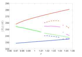
Figure 1: Bifurcation diagram for the model studied in Lucarini and Bódai (2017) for the long term, globally averaged ocean temperature $[\langle T_{S}\rangle]$. Bistability is found for a large range of values of the control parameter $\mu$. Of interest here: red line: warm (W) states; blue line: Snowball (SB) state; green line: Melancholia (M) states, (constructed via the edge tracking algorithm). The $W\rightarrow SB$ ($SB\rightarrow W$) tipping point is located at $\mu_{W\rightarrow SB}\sim 0.965$ ($\mu_{SB\rightarrow W}\sim 1.06$).

In Bódai et al. (2014); Lucarini and Bódai (2017), we adapted the edge tracking algorithm presented in Skufca et al. (2006); Schneider et al. (2007) and constructed in the bistable region the M states separating the two co-existing realisable W and SB climates. The critical transitions are associated to boundary crises Ott (2002) associated to collisions between the M state and one of the stable climates, and are flagged by a diverging linear response Tantet et al. (2018). In Lucarini and Bódai (2017) we constructed the M states for an intermediate complexity climate model with O($10^{5}$) degrees of freedom. We showed that the M state has, in a range of values of the control parameter $\mu$ ( ratio between the considered solar irradiance and the present-day value), chaotic dynamics, leading to weather variability and to a limited horizon of predictability; see the caption of Fig. 1. Since this instability is much faster than the climatic one due to the ice-albedo feedback, the basin boundary is a fractal set with near-zero codimension, in agreement with results obtained in low-dimensional cases Grebogi et al. (1983); Lai and Tél (2011). Near the basin boundary there is de facto no Lorenz’ Lorenz (1975) predictability of the second kind.

Here, building on Lucarini and Bódai (2017), we study how a fluctuating solar irradiance can trigger transitions between the W and SB states, and investigate the typical paths of such transitions. The climate model is constructed by coupling the primitive equations atmospheric model PUMA Frisius et al. (1998) with the Ghil-Sellers energy balance model Ghil (1976) (see also Schneider and Gal-Chen (1973); Dwyer and Petersen (1973)), which describes succinctly oceanic heat transports. The ocean model describes effectively the ice-albedo feedback, and defines the slow manifold of the system. The coupling is realised by relaxing the atmospheric temperature to an adiabatic profile anchored to the ocean surface temperature, and by incorporating vertical heat fluxes. The ocean temperature $T_{S}(t,\phi,\lambda)$, where $\phi$ is latitude and $\lambda$ is longitude, evolves as follows:

$$C(\phi)\frac{\partial T_{S}}{\partial t} =\mu(1+\sigma\frac{dW}{dt})I(\phi)\frac{S^{*}}{4}(1-\alpha(\phi,T_{S}))-O(T_{S})$$

$$-D_{\phi}[T_{S}]+\chi[T_{S},T_{A}],$$ (1)

where $S^{*}$ is the present-day solar irradiance (the factor 4 comes from the Earth-Sun geometry Saltzman (2001)), and the heat capacity $C$ and the geometrical factor $I$ depend explicitly on $\phi$. The albedo $\alpha$ depends on $\phi$ and, critically, on $T_{S}$, with a rapid transition from high albedo for low values of $T_{S}$ ($\alpha_{max}=0.6$) to low albedo for $T_{S}\gtrsim 260$ $K$ ($\alpha_{min}=0.2$), which fuels the ice-albedo feedback. Finally, $O$ is the outgoing radiation, , and increases with $T_{S}$, (accounting for the Boltzmann feedback beside the greenhouse effect), $D$ is a diffusion operator parametrizing the meridional heat transport, and $\chi$ describes the ocean-atmosphere heat exchange Lucarini and Bódai (2017).

The stochastic perturbation modulates the solar irradiance through the factor $(1+\sigma dW/dt)$, where $\sigma$ controls the noise intensity noise, and $dW$ is the increment of a Wiener process. The noise is multiplicative because $dW/dt$ is multiplied by the factor $1-\alpha(\phi,T_{S})$ in Eq. 1. Adding a Gaussian random variable of variance $\sigma_{0}$ at each time step $\Delta t$ ($1$ hour), when numerically integrating the model, corresponds to having a relative fluctuation of the solar irradiance $\sigma_{\tau}=\sigma_{0}/\sqrt{N}$ on the time scale $\tau=N\times\Delta t$.

Noise-induced escapes from attractors have been intensely studied Hanggi (1986); Kautz (1987); Grassberger (1989). We frame our problem by considering a stochastic differential equation in Itô form written as ${d{\bm{x}}(t)}=\bm{F}(\bm{x(t)})dt+\sigma\bm{s}(\bm{x})d\bm{W}$, where $\dot{\bm{x}}(t)=\bm{F}(\bm{x(t)})$ has multiple steady states, $d\bm{W}$ is the increment of an $M-$dimensional Wiener process, $\bm{s}(\bm{x})^{T}\bm{s}(\bm{x})$ is the noise covariance matrix with $\bm{s}(\bm{x})\in\mathbb{R}^{N\times M}$, and $\sigma\geq 0$. In the case of non-degenerate additive noise and for a class of multiplicative noise laws, the Freidlin-Wentzell Freidlin and Wentzell (1984) theory and extensions thereof Graham et al. (1991); Hamm et al. (1994); Lai and Tél (2011) show that in the weak-noise limit $\sigma\rightarrow 0$ the invariant measure can be written as a large deviation law:

$$W_{\sigma}(\bm{x})\sim Z(\bm{x})\exp\left(-\frac{2\Phi(\bm{x})}{\sigma^{2}}\right),$$ (2)

where $Z(\bm{x})$ is the pre-exponential factor and $\Phi(\bm{x})$ is the pseudo-potential , which has local minima at the deterministic attractors $\Omega_{j}$, $j=1,\ldots,J$. Both the M states and the attractors can be chaotic: if so, $\Phi$ has constant value over each M state and each attractor, respectively Graham et al. (1991); Hamm et al. (1994). The probability that an orbit with initial condition in $B_{j}$ does not escape from it over a time $p$ decays as:

$$P(p)=\frac{1}{\bar{\tau}_{\sigma}}\exp\left(-\frac{p}{\bar{\tau}_{\sigma}}\right),\quad\bar{\tau}_{\sigma}\propto\exp\left(\frac{2\Delta\Phi}{\sigma^{2}}\right)$$ (3)

where $\bar{\tau}_{\sigma}$ is the expected escape time and where $\Delta\Phi=\Phi(\Pi_{l})-\Phi(\Omega_{j})$ is the pseudo-potential barrier height Lai and Tél (2011); In general, one may need to add a correcting prefactor in Eq. 3 Lai and Tél (2011). In the weak-noise limit, the transition paths follow the instantons, which are minimizers of the Freidlin-Wentzell action Kautz (1987); Grassberger (1989); Kraut and Feudel (2002); Beri et al. (2005). An instanton connects a point in $\Omega_{j}$ to a point in $\Pi_{l}$; if these sets are not fixed points, the instanton is not unique, as the pseudo-potential is constant on $\Omega_{j}$ and $\Pi_{l}$.

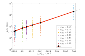
Figure 2: Escape times for the $W\rightarrow SB$ transitions for various noise strengths. Each dot corresponds to an observed escape time. The slope of the straight line fit is twice the quantity $\Delta\Phi$, see Eq. 3. An optimal algorithm for estimating $\Delta\Phi$ is reported in Bódai (2018).

The results given in Eqs. 2-3 apply in the case of multiplicative noise laws if one assumes that the noise correlation matrix is well-behaved, according to what discussed in Lindley and Schwartz (2013); Tang et al. (2017). We believe that in our system such a condition applies, essentially because the factor $1-\alpha(\phi,T_{S})$ is bounded in the phase space between 0.4 ($\alpha=\alpha_{max}=0.6$, ice-cover) and 0.8 ($\alpha=\alpha_{min}=0.2$, very warm conditions with absence of ice cover). In the phase space region near the SB attractor, we have that $1-\alpha(\phi,T_{S})\sim 0.4$ since the temperature $T_{S}$ is extremely low and the planet is fully glaciated, so that $\alpha(\phi,T_{S})$ is constant, with $\alpha(\phi,T_{S})\sim\alpha_{min}$. Near the W attractor, the properties of $\alpha(\phi,T_{S})$ are more complex, because only part of the planet is glaciated. If $[X]$ the global average of the spatial field $X$, and $\langle Y\rangle$ is the long term average of $Y$, we have that, typically, $\partial[\langle\alpha\rangle]/\partial[\langle{T}_{S}\rangle]<0$, because a decrease in $[\langle T_{S}\rangle]$ leads to moving the ice line equatorward, thus leading to higher average albedo. Then, near the W attractor, noise enhances the instability linked to the $W\rightarrow SB$ transition, and one expects that for finite noise the peak of the invariant measure is shifted to lower values of $[T_{S}]$ with respect to the deterministic attractor.

The ratio of the variance of the noise in the W vs SB attractors can be estimated as $\approx((1-\alpha_{W})/(1-\alpha_{SB}))^{2}\approx 3$, where the typical albedo of the W (SB) attractor is $\alpha_{W}\approx 0.3$ ($\alpha_{SB}\approx\alpha_{max}=0.6$). The two attractors have different microscopic (and macroscopic) temperatures.

We show now our results. We treat two cases inside the region of bistability depicted in Fig. 1, namely $\mu=0.98$ (close to the tipping point $\mu_{W\rightarrow SB}$) and $\mu=1.0$.

In the case of $\mu=0.98$, we consider noise intensities ranging from $\sigma_{\tau}=0.5\%$ to $\sigma_{\tau}=1.4\%$, with $\tau=100$ $years$ ($y$). For each value of $\sigma_{\tau}$, we initialise 50 orbits in the W basin of attraction and study the statistics of the escape times towards the SB attractor. When the transition takes place, we stop the integration. We observe (not shown) that for each value of $\sigma_{\tau}$ the escape times are to a good approximation exponentially distributed, see Eq. 3. The expectation value of the transition times $\bar{\tau}_{\sigma}$ is shown in Fig. 2. Indeed, $\bar{\tau}_{\sigma}$ obeys to a good approximation what shown in Eq. 3, so that the difference of the potential $\Phi$ is half of the slope of the straight line. For reference, we have that for $\sigma_{100y}=0.5\%$ the average escape time is about $5.2\times 10^{3}$ $y$. We can predict that the escape rate increases to about $1.2\times 10^{7}$ $y$ when $\sigma_{100y}\sim 0.3\%$.

We then look at the transition paths. Following Bódai et al. (2014); Lucarini and Bódai (2017), we choose to consider the reduced phase space spanned by $[T_{S}]$ and by $\Delta T_{S}$, which is the difference between the spatial averages of $T_{S}$ in the latitudinal belts $[0,30^{\circ}N]$ and $[30^{\circ}N,90^{\circ}N]$, respectively. This reduced phase space provides a minimal yet physically informative viewpoint on the problem. Figure 3 depicts ($\sigma_{\tau}=1.0\%$), the transient two-dimensional probability distribution function (pdf) $\tilde{\rho}$ constructed using the above-described 50 simulations, where the statistics is collected only until the $W\rightarrow SB$ transition is realised. Note that $\tilde{\rho}$ is not the invariant density of the system. The transitions typically take place along a very narrow band linking the W attractor and the M state . We construct an estimate of the instanton associated to the $W\rightarrow SB$ transition by conditionally averaging the orbits according to the value of $[T_{S}]$. To a good approximation, the instanton connects the W attractor to the M state, and follows a path of decreasing probability. We remark that we do not find evidence of different paths for escape vs relaxation trajectories, which, instead, is a signature of non-equilibrium Zinn-Justin (1996). This can be explained by considering that, as discussed in Bódai et al. (2014), the ocean model evolves approximately in an energy landscape.

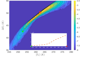
Figure 3: Main graph: Logarithm of $\tilde{\rho}$ projected onto $(T_{S},[\Delta T_{S}])$ for $\mu=0.98$; W attractor (red dot); M state (green dot). We have used $\sigma_{100y}=1\%$. The $W\rightarrow SB$ instanton (red dashed line) is indicated. Bottom right inset: probability along the instanton.

When $\mu=0.98$, the $SB\rightarrow W$ transitions are rather rare unless one considers relatively large values of $\sigma$. This is due to the much lower value of $\Phi$ at the SB attractor than at the W attractor (see Eq. 3), so that (see Eq. 2) the fraction of the invariant measure supported near the W attractor is extremely small. We focus next on the case of $\mu=1.0$, where the population is split more evenly between the W and SB attractors. We are then able to construct for each value of $\sigma_{\tau}$ the invariant measure using a single orbit of the system, provided we can observe a sufficient number of transitions. We use $\sigma_{100y}=1.5\%$. Our results are shown in Fig. 4 for a trajectory lasting $\approx 6.0\times 10^{4}$ $y$ and characterised by 92 $SB\rightarrow W$ and $W\rightarrow SB$ transitions, whose average rates are consistent with an occupation of about $35\%$ for the $W$ basin of attraction, and of about $65\%$ for the $SB$ basin of attraction. The projection of the invariant measure on the $([T_{S}],\Delta T_{S})$ plane shows that the peaks of the pdfs are very close to the $W$ and $SB$ attractors (note the predicted slight shift for the $W$ case, visible because the noise is stronger than in Fig. 3), and that the agreement further improves when considering the two marginal pdfs (top left and bottom right insets). We can construct both the $W\rightarrow SB$ and the $SB\rightarrow W$ instantons, whose starting and final points agree remarkably well with the attractors and the M state. We discover that the instantons follow a path of monotonic descent, following closely the crests of the pdf), with the minimum at the M state. We also run a simulation lasting $\approx 2.7\times 10^{4}$ $y$ using $\sigma_{100y}=1.8\%$. We obtain 73 $SB\rightarrow W$ and $W\rightarrow SB$ transitions. Comparing the statistics of this run with what is shown in Fig. 4, we find good agreement with the predictions of Eqs. 2-3 (not shown).

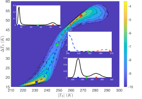
Figure 4: Main graph: $\rho$ in the projected phase space $(T_{S},[\Delta T_{S}])$. W attractor (red dot), SB attractor (blue dot), M state (green dot) for $\mu=1$. Red (blue) dashed line: $W\rightarrow SB$ ($SB\rightarrow W$) instanton. We have used $\sigma_{100y}=1.5\%$. Top left inset: marginal pdf with respect to $\Delta T_{S}$. Bottom right inset: marginal pdf with respect to $[T_{S}]$. Center right inset: probability along the two instantons.

Concluding, in this letter we have studied the problem of noise-induced transitions between the W and the SB state of the climate system using a intermediate complexity stochastic model. The deterministic version of this model had been used to construct the M states for a vast range of values of the solar irradiance Lucarini and Bódai (2017). Including stochastic perturbations allows for exploring the phase space of the system. We have chosen to study the impact of fluctuations in the solar irradiance, which entails adding a multiplicative noise. In particular, the SB climate reflects more radiation because large ice-covered surfaces lead to higher albedo, so that the effective noise will be weaker than the one acting near the W attractor. We have explained why a large deviation theory-based mathematical framework is able to explain very satisfactorily our results. We show that one can construct the pseudo-potential defining the escape rate from the basins of attraction and the natural measure of the stochastically perturbed system. In future investigations we plan to extend the analysis performed here to values of $\mu$ covering the whole range of bistability, in order to understanding how the pseudo-potential depends on $\mu$. Using a low-dimensional projection of the invariant measure, we show that the instantons connect the attractors with the M states, following a path of steepest descent. This gives a key connection between the stochastic and the deterministic points of view on study of the multistability of the climate.

A further link between the stochastically perturbed and deterministic system can be described as follows. If we consider values of $\mu$ just below the critical one $\mu_{W\rightarrow SB}\sim 0.965$ defining the $W\rightarrow SB$ tipping point, one can find long-lived transient chaotic trajectories. It is worth investigating whether such transients are associated to a invariant saddle emerging as a result of the boundary crisis. We have observed that the way such long-lived trajectories collapse to the SB state is very similar to the way, when $\mu=0.98$, stochastically perturbed orbits initialised in the W state basin of attraction perform the transition. In future studies we will explore such similarity looking into the possible presence of a ghost state Medeiros et al. (2017).

The knowledge of M states is key to understanding tipping points. When an attractor and a M states are nearby, the system’s response to perturbations diverges, as the correlations decay very slowly Tantet et al. (2018). These findings extend and generalise the classical point of view given in Lenton and et al. (2008). What is proposed here, combined with the framework given in Ashwin et al. (2012), could be key for understanding and predicting the criticalities in the trajectories of the Earth system Steffen and et al. (2018), including those leading to very hot, non-habitable conditions Gomez-Leal et al. (2018). A tipping element we will investigate along the lines of the present study is the Atlantic meridional overturning circulation Lenton and et al. (2008).

References

- Hoffman and Schrag (2002) P. F. Hoffman and D. P. Schrag, Terra Nova 14, 129 (2002).
- Pierrehumbert et al. (2011) R. T. Pierrehumbert, D. Abbot, A. Voigt, and D. Koll, Ann. Rev, Earth Plan. Sci. 39, 417 (2011).
- Donnadieu et al. (2014) Y. Donnadieu, Y. Goddéris, and G. L. Hir, in Treatise on Geochemistry, edited by H. D. Holland and K. K. Turekian (Elsevier, Oxford, 2014) pp. 217 – 229.
- Budyko (1969) M. Budyko, Tellus 21, 611 (1969).
- Sellers (1969) W. Sellers, J. Appl. Meteorol. 8, 392 (1969).
- Ghil (1976) M. Ghil, J. Atmos. Sci. 33, 3 (1976).
- Lucarini et al. (2013) V. Lucarini, S. Pascale, R. Boschi, E. Kirk, and N. Iro, Astr. Nach. 334, 576 (2013).
- Boschi et al. (2013) R. Boschi, V. Lucarini, and S. Pascale, Icarus 227, 1724 (2013).
- Lucarini and Bódai (2017) V. Lucarini and T. Bódai, Nonlinearity 30, R32 (2017).
- Feudel et al. (2018) U. Feudel, A. N. Pisarchik, and K. Showalter, Chaos: An Interdisciplinary Journal of Nonlinear Science 28, 033501 (2018).
- Lenton and et al. (2008) T. Lenton and et al., Proceedings of the National Academy of Sciences 105, 1786 (2008).
- Grebogi et al. (1983) C. Grebogi, E. Ott, and J. A. Yorke, Phys. Rev. Lett. 50, 935 (1983).
- Robert et al. (2000) C. Robert, K. T. Alligood, E. Ott, and J. A. Yorke, Physica D: Nonlinear Phenomena 144, 44 (2000).
- Ott (2002) E. Ott, Chaos in Dynamical Systems (Cambridge University Press, 2002).
- Vollmer et al. (2009) J. Vollmer, T. M. Schneider, and B. Eckhardt, New Journal of Physics 11, 013040 (2009).
- Bódai et al. (2014) T. Bódai, V. Lucarini, F. Lunkeit, and R. Boschi, Clim. Dyn. 44, 3361 (2014).
- Skufca et al. (2006) J. D. Skufca, J. A. Yorke, and B. Eckhardt, Phys. Rev. Lett. 96, 174101 (2006).
- Schneider et al. (2007) T. M. Schneider, B. Eckhardt, and J. A. Yorke, Phys. Rev. Lett. 99, 034502 (2007).
- Tantet et al. (2018) A. Tantet, V. Lucarini, F. Lunkeit, and H. A. Dijkstra, Nonlinearity 31, 2221 (2018).
- Lai and Tél (2011) Y.-C. Lai and T. Tél, Transient Chaos (Springer, New York, 2011).
- Lorenz (1975) E. N. Lorenz, in GARP Publication Series (WMO, 1975) pp. 132–136.
- Frisius et al. (1998) T. Frisius, F. Lunkeit, K. Fraedrich, and I. N. James, Quarterly Journal of the Royal Meteorological Society 124, 1019 (1998).
- Schneider and Gal-Chen (1973) S. H. Schneider and T. Gal-Chen, Journal of Geophysical Research 78, 6182 (1973).
- Dwyer and Petersen (1973) H. A. Dwyer and T. Petersen, J. Appl. Meteo. 12, 36 (1973).
- Saltzman (2001) B. Saltzman, Dynamical Paleoclimatology (Academic Press New York, 2001).
- Hanggi (1986) P. Hanggi, Journal of Statistical Physics 42, 105 (1986).
- Kautz (1987) R. Kautz, Physics Letters A 125, 315 (1987).
- Grassberger (1989) P. Grassberger, J. Phys. A 22, 3283 (1989).
- Freidlin and Wentzell (1984) M. I. Freidlin and A. Wentzell, Random Perturbations of Dynamical Systems (Springer, New York, 1984).
- Graham et al. (1991) R. Graham, A. Hamm, and T. Tél, Phys. Rev. Lett. 66, 3089 (1991).
- Hamm et al. (1994) A. Hamm, T. Tél, and R. Graham, Phys. Lett. A 185, 313 (1994).
- Kraut and Feudel (2002) S. Kraut and U. Feudel, Phys. Rev. E 66, 015207 (2002).
- Beri et al. (2005) S. Beri, R. Mannella, D. G. Luchinsky, A. N. Silchenko, and P. V. E. McClintock, Phys. Rev. E 72, 036131 (2005).
- Bódai (2018) T. Bódai, ArXiv e-prints , arXiv:1808.06903 (2018).
- Lindley and Schwartz (2013) B. S. Lindley and I. B. Schwartz, Physica D 255, 22 (2013).
- Tang et al. (2017) Y. Tang, R. Yuan, G. Wang, X. Zhu, and P. Ao, Scientific Reports 7, 15762 (2017).
- Zinn-Justin (1996) J. Zinn-Justin, Quantum Field Theory and Critical Phenomena (Oxford University Press, Oxford, 1996).
- Medeiros et al. (2017) E. S. Medeiros, I. Caldas, M. S. Baptista, and U. Feudel, Scientific Reports 7, 42351 EP (2017).
- Ashwin et al. (2012) P. Ashwin, S. Wieczorek, R. Vitolo, and P. Cox, Philosophical Transactions of the Royal Society of London A: Mathematical, Physical and Engineering Sciences 370, 1166 (2012).
- Steffen and et al. (2018) W. Steffen and et al., Proceedings of the National Academy of Sciences 115, 8252 (2018).
- Gomez-Leal et al. (2018) I. Gomez-Leal, L. Kaltenegger, V. Lucarini, and F. Lunkeit, Icarus (2018), https://doi.org/10.1016/j.icarus.2018.11.019.