ACVAE-VC: Non-parallel many-to-many voice conversion with
auxiliary classifier variational autoencoder

Abstract

This paper proposes a non-parallel many-to-many voice conversion (VC) method using a variant of the conditional variational autoencoder (VAE) called an auxiliary classifier VAE (ACVAE). The proposed method has three key features. First, it adopts fully convolutional architectures to construct the encoder and decoder networks so that the networks can learn conversion rules that capture time dependencies in the acoustic feature sequences of source and target speech. Second, it uses an information-theoretic regularization for the model training to ensure that the information in the attribute class label will not be lost in the conversion process. With regular CVAEs, the encoder and decoder are free to ignore the attribute class label input. This can be problematic since in such a situation, the attribute class label will have little effect on controlling the voice characteristics of input speech at test time. Such situations can be avoided by introducing an auxiliary classifier and training the encoder and decoder so that the attribute classes of the decoder outputs are correctly predicted by the classifier. Third, it avoids producing buzzy-sounding speech at test time by simply transplanting the spectral details of the input speech into its converted version. Subjective evaluation experiments revealed that this simple method worked reasonably well in a non-parallel many-to-many speaker identity conversion task.

Index Terms—  Voice conversion (VC), variational autoencoder (VAE), non-parallel VC, auxiliary classifier VAE (ACVAE), fully convolutional network

1 Introduction

Voice conversion (VC) is a technique for converting para/non-linguistic information contained in a given utterance without changing the linguistic information. This technique can be applied to various tasks such as speaker-identity modification for text-to-speech (TTS) systems [1], speaking assistance [2, 3], speech enhancement [4, 5, 6], and pronunciation conversion [7].

One widely studied VC framework involves Gaussian mixture model (GMM)-based approaches [8, 9, 10]. Recently, neural network (NN)-based frameworks based on restricted Boltzmann machines [11, 12], feed-forward deep NNs [13, 14], recurrent NNs [15, 16], variational autoencoders (VAEs) [17, 18, 19] and generative adversarial nets (GANs) [7], and an exemplar-based framework based on non-negative matrix factorization (NMF) [20, 21] have also attracted particular attention. While many VC methods including those mentioned above require accurately aligned parallel data of source and target speech, in general scenarios, collecting parallel utterances can be a costly and time-consuming process. Even if we were able to collect parallel utterances, we typically need to perform automatic time alignment procedures, which becomes relatively difficult when there is a large acoustic gap between the source and target speech. Since many frameworks are weak with respect to the misalignment found with parallel data, careful pre-screening and manual correction is often required to make these frameworks work reliably. To sidestep these issues, this paper aims to develop a non-parallel VC method that requires no parallel utterances, transcriptions, or time alignment procedures.

The quality and conversion effect obtained with non-parallel methods are generally poorer than with methods using parallel data since there is a disadvantage related to the training condition. Thus, it would be challenging to achieve as high a quality and conversion effect with non-parallel methods as with parallel methods. Several non-parallel methods have already been proposed [18, 19, 22, 23]. For example, a method using automatic speech recognition (ASR) was proposed in [22] where the idea is to convert input speech under a restriction, namely that the posterior state probability of the acoustic model of an ASR system is preserved. Since the performance of this method depends heavily on the quality of the acoustic model of ASR, it can fail to work if ASR does not function reliably. A method using i-vectors [24], which is known to be a powerful feature for speaker verification, was proposed in [23] where the idea is to shift the acoustic features of input speech towards target speech in the i-vector space so that the converted speech is likely to be recognized as the target speaker by a speaker recognizer. While this method is also free of parallel data, one limitation is that it is applicable only to speaker identity conversion tasks.

Recently, a framework based on conditional variational autoencoders (CVAEs) [25, 26] was proposed in [18, 27]. As the name implies, VAEs are a probabilistic counterpart of autoencoders (AEs), consisting of encoder and decoder networks. Conditional VAEs (CVAEs) [26] are an extended version of VAEs with the only difference being that the encoder and decoder networks take an attribute class label $c$ as an additional input. By using acoustic features associated with attribute labels as the training examples, the networks learn how to convert an attribute of source speech to a target attribute according to the attribute label fed into the decoder. While this VAE-based VC approach is notable in that it is completely free of parallel data and works even with unaligned corpora, there are three major drawbacks. Firstly, the devised networks are designed to produce acoustic features frame-by-frame, which makes it difficult to learn time dependencies in the acoustic feature sequences of source and target speech. Secondly, one well-known problem as regards VAEs is that outputs from the decoder tend to be oversmoothed. This can be problematic for VC applications since it usually results in poor quality buzzy-sounding speech. One natural way of alleviating the oversmoothing effect in VAEs would be to use the VAE-GAN framework [28]. A non-parallel VC method based on this framework has already been proposed in [19]. With this method, an adversarial loss derived using a GAN discriminator is incorporated into the training loss to make the decoder outputs of a CVAE indistinguishable from real speech features. While this method is able to produce more realistic-sounding speech than the regular VAE-based method [18], as will be shown in Section 4, the audio quality and conversion effect are still limited. Thirdly, in the regular CVAEs, the encoder and decoder are free to ignore the additional input $c$ by finding networks that can reconstruct any data without using $c$. In such a situation, the attribute class label $c$ will have little effect on controlling the voice characteristics of the input speech.

To overcome these drawbacks and limitations, in this paper we describe three modifications to the conventional VAE-based approach. First, we adopt fully convolutional architectures to design the encoder and decoder networks so that the networks can learn conversion rules that capture short- and long-term dependencies in the acoustic feature sequences of source and target speech. Secondly, we propose simply transplanting the spectral details of input speech into its converted version at test time to avoid producing buzzy-sounding speech. We will show in Section 4 that this simple method works considerably better than the VAE-GAN framework [19] in terms of audio quality. Thirdly, we propose using an information-theoretic regularization for the model training to ensure that the attribute class information will not be lost in the conversion process. This can be done by introducing an auxiliary classifier whose role is to predict to which attribute class an input acoustic feature sequence belongs and by training the encoder and decoder so that the attribute classes of the decoder outputs are correctly predicted by the classifier. We call the present VAE variant an auxiliary classifier VAE (or ACVAE).

2 VAE voice conversion

2.1 Variational Autoencoder (VAE)

VAEs [25, 26] are stochastic neural network models consisting of encoder and decoder networks. The encoder network generates a set of parameters for the conditional distribution $q_{\phi}(\bm{\mathbf{z}}|\bm{\mathbf{x}})$ of a latent space variable $\bm{\mathbf{z}}$ given input data $\bm{\mathbf{x}}$, whereas the decoder network generates a set of parameters for the conditional distribution $p_{\theta}(\bm{\mathbf{x}}|\bm{\mathbf{z}})$ of the data $\bm{\mathbf{x}}$ given the latent space variable $\bm{\mathbf{z}}$. Given a training dataset ${\mathcal{S}}=\{\bm{\mathbf{x}}_{m}\}_{m=1}^{M}$, VAEs learn the parameters of the entire network so that the encoder distribution $q_{\phi}(\bm{\mathbf{z}}|\bm{\mathbf{x}})$ becomes consistent with the posterior $p_{\theta}(\bm{\mathbf{z}}|\bm{\mathbf{x}})\propto p_{\theta}(\bm{\mathbf{x}}|\bm{\mathbf{z}})p(\bm{\mathbf{z}})$. By using Jensen’s inequality, the log marginal distribution of data $\bm{\mathbf{x}}$ can be lower-bounded by

$$\log p_{\theta}(\bm{\mathbf{x}}) =\log\int q_{\phi}(\bm{\mathbf{z}}|\bm{\mathbf{x}})\frac{p_{\theta}(\bm{\mathbf{x}}|\bm{\mathbf{z}})p(\bm{\mathbf{z}})}{q_{\phi}(\bm{\mathbf{z}}|\bm{\mathbf{x}})}d\bm{\mathbf{z}}$$

$$\geq\int q_{\phi}(\bm{\mathbf{z}}|\bm{\mathbf{x}})\log\frac{p_{\theta}(\bm{\mathbf{x}}|\bm{\mathbf{z}})p(\bm{\mathbf{z}})}{q_{\phi}(\bm{\mathbf{z}}|\bm{\mathbf{x}})}d\bm{\mathbf{z}}$$ (1)

$$=\mathbb{E}_{\bm{\mathbf{z}}\sim q_{\phi}(\bm{\mathbf{z}}|\bm{\mathbf{x}})}[\log p_{\theta}(\bm{\mathbf{x}}|\bm{\mathbf{z}})]-{\rm KL}[q_{\phi}(\bm{\mathbf{z}}|\bm{\mathbf{x}})\|p(\bm{\mathbf{z}})],$$

where the difference between the left- and right-hand sides of this inequality is equal to the Kullback-Leibler divergence ${\rm KL}[q_{\phi}(\bm{\mathbf{z}}|\bm{\mathbf{x}})\|p_{\theta}(\bm{\mathbf{z}}|\bm{\mathbf{x}})]$, which is minimized when

$$q_{\phi}(\bm{\mathbf{z}}|\bm{\mathbf{x}})=p_{\theta}(\bm{\mathbf{z}}|\bm{\mathbf{x}}).$$ (2)

This means we can make $q_{\phi}(\bm{\mathbf{z}}|\bm{\mathbf{x}})$ and $p_{\theta}(\bm{\mathbf{z}}|\bm{\mathbf{x}})\propto p_{\theta}(\bm{\mathbf{x}}|\bm{\mathbf{z}})p(\bm{\mathbf{z}})$ consistent by maximizing the lower bound of (1). One typical way of modeling $q_{\phi}(\bm{\mathbf{z}}|\bm{\mathbf{x}})$, $p_{\theta}(\bm{\mathbf{x}}|\bm{\mathbf{z}})$ and $p(\bm{\mathbf{z}})$ is to assume Gaussian distributions

$$q_{\phi}(\bm{\mathbf{z}}|\bm{\mathbf{x}}) =\mathcal{N}(\bm{\mathbf{z}}|{\bm{\mu}}_{\phi}(\bm{\mathbf{x}}),{\rm diag}({\bm{\sigma}}_{\phi}^{2}(\bm{\mathbf{x}}))),$$ (3)

$$p_{\theta}(\bm{\mathbf{x}}|\bm{\mathbf{z}}) =\mathcal{N}(\bm{\mathbf{x}}|{\bm{\mu}}_{\theta}(\bm{\mathbf{z}}),{\rm diag}({\bm{\sigma}}_{\theta}^{2}(\bm{\mathbf{z}}))),$$ (4)

$$p(\bm{\mathbf{z}}) =\mathcal{N}(\bm{\mathbf{z}}|{\bf 0},{\bf I}),$$ (5)

where ${\bm{\mu}}_{\phi}(\bm{\mathbf{x}})$ and ${\bm{\sigma}}_{\phi}^{2}(\bm{\mathbf{x}})$ are the outputs of an encoder network with parameter $\phi$, and ${\bm{\mu}}_{\theta}(\bm{\mathbf{z}})$ and ${\bm{\sigma}}_{\theta}^{2}(\bm{\mathbf{z}})$ are the outputs of a decoder network with parameter $\theta$. The first term of the lower bound can be interpreted as an autoencoder reconstruction error. By using a reparameterization $\bm{\mathbf{z}}={\bm{\mu}}_{\phi}(\bm{\mathbf{x}})+{\bm{\sigma}}_{\phi}(\bm{\mathbf{x}})\odot{\bm{\epsilon}}$ with ${\bm{\epsilon}}\sim\mathcal{N}({\bm{\epsilon}}|{\mathbf{0}},{\mathbf{I}})$, sampling $\bm{\mathbf{z}}$ from $q_{\phi}(\bm{\mathbf{z}}|\bm{\mathbf{x}})$ can be replaced by sampling ${\bm{\epsilon}}$ from the distribution, which is independent of $\theta$. This allows us to compute the gradient of the lower bound with respect to $\theta$ by using a Monte Carlo approximation of the expectation $\mathbb{E}_{\bm{\mathbf{z}}\sim q_{\phi}(\bm{\mathbf{z}}|\bm{\mathbf{x}})}[\cdot]$. The second term is given as the negative KL divergence between $q_{\phi}(\bm{\mathbf{z}}|\bm{\mathbf{x}})$ and $p(\bm{\mathbf{z}})=\mathcal{N}(\bm{\mathbf{z}}|{\mathbf{0}},{\mathbf{I}})$. This term can be interpreted as a regularization term that forces each element of the encoder output to be uncorrelated and normally distributed.

Conditional VAEs (CVAEs) [26] are an extended version of VAEs with the only difference being that the encoder and decoder networks can take an auxiliary variable $c$ as an additional input. With CVAEs, (3) and (4) are replaced with

$$q_{\phi}(\bm{\mathbf{z}}|\bm{\mathbf{x}},c) =\mathcal{N}(\bm{\mathbf{z}}|{\bm{\mu}}_{\phi}(\bm{\mathbf{x}},c),{\rm diag}({\bm{\sigma}}_{\phi}^{2}(\bm{\mathbf{x}},c))),$$ (6)

$$p_{\theta}(\bm{\mathbf{x}}|\bm{\mathbf{z}},c) =\mathcal{N}(\bm{\mathbf{x}}|{\bm{\mu}}_{\theta}(\bm{\mathbf{z}},c),{\rm diag}({\bm{\sigma}}_{\theta}^{2}(\bm{\mathbf{z}},c))),$$ (7)

and the variational lower bound to be maximized becomes

$$\mathcal{J}(\phi,\theta)= \mathbb{E}_{(\bm{\mathbf{x}},c)\sim p_{\rm D}(\bm{\mathbf{x}},c)}\big{[}\mathbb{E}_{\bm{\mathbf{z}}\sim q(\bm{\mathbf{z}}|\bm{\mathbf{x}},c)}[\log p(\bm{\mathbf{x}}|\bm{\mathbf{z}},c)]$$

$$~{}~{}~{}~{}~{}~{}~{}~{}~{}~{}~{}~{}~{}~{}~{}~{}~{}~{}~{}~{}~{}~{}~{}~{}~{}~{}~{}~{}~{}~{}-{\rm KL}[q(\bm{\mathbf{z}}|\bm{\mathbf{x}},c)\|p(\bm{\mathbf{z}})]\big{]},$$ (8)

where $\mathbb{E}_{(\bm{\mathbf{x}},c)\sim p_{\rm D}(\bm{\mathbf{x}},c)}[\cdot]$ denotes the sample mean over the training examples $\{\bm{\mathbf{x}}_{m},c_{m}\}_{m=1}^{M}$.

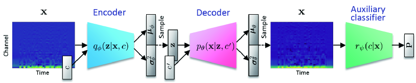
Fig. 1: Illustration of ACVAE-VC.

2.2 Non-parallel voice conversion using CVAE

By letting $\bm{\mathbf{x}}\in\mathbb{R}^{Q}$ and $c$ be an acoustic feature vector and an attribute class label, a non-parallel VC problem can be formulated using the CVAE [18, 19]. Given a training set of acoustic features with attribute class labels $\{\bm{\mathbf{x}}_{m},c_{m}\}_{m=1}^{M}$, the encoder learns to map an input acoustic feature $\bm{\mathbf{x}}$ and an attribute class label $c$ to a latent space variable $\bm{\mathbf{z}}$ (expected to represent phonetic information) and then the decoder reconstructs an acoustic feature $\hat{\bm{\mathbf{x}}}$ conditioned on the encoded latent space variable $\bm{\mathbf{z}}$ and the attribute class label $c$. At test time, we can generate a converted feature by feeding an acoustic feature of the input speech into the encoder and a target attribute class label into the decoder.

3 Proposed method

3.1 Fully Convolutional VAE

While the model in [18, 19] is designed to convert acoustic features frame-by-frame and fails to learn conversion rules that reflect time-dependencies in acoustic feature sequences, we propose extending it to a sequential version to overcome this limitation. Namely, we devise a CVAE that takes an acoustic feature sequence instead of a single-frame acoustic feature as an input and outputs an acoustic feature sequence of the same length. Hence, in the following we assume that $\bm{\mathbf{x}}\in\mathbb{R}^{Q\times N}$ is an acoustic feature sequence of length $N$. While RNN-based architectures are a natural choice for modeling time series data, we use fully convolutional networks to design $q_{\phi}$ and $p_{\theta}$, as detailed in 3.4.

3.2 Auxiliary Classifier VAE

We hereafter assume that a class label comprises one or more categories, each consisting of multiple classes. We thus represent $c$ as a concatenation of one-hot vectors, each of which is filled with 1 at the index of a class in a certain category and with 0 everywhere else. For example, if we consider speaker identities as the only class category, $c$ will be represented as a single one-hot vector, where each element is associated with a different speaker.

The regular CVAEs impose no restrictions on the manner in which the encoder and decoder may use the attribute class label $c$. Hence, the encoder and decoder are free to ignore $c$ by finding distributions satisfying $q_{\phi}(\bm{\mathbf{z}}|\bm{\mathbf{x}},c)=q_{\phi}(\bm{\mathbf{z}}|\bm{\mathbf{x}})$ and $p_{\theta}(\bm{\mathbf{x}}|\bm{\mathbf{z}},c)=p_{\theta}(\bm{\mathbf{x}}|\bm{\mathbf{z}})$. This can occur for instance when the encoder and decoder have sufficient capacity to reconstruct any data without using $c$. In such a situation, $c$ will have little effect on controlling the voice characteristics of input speech. To avoid such situations, we introduce an information-theoretic regularization [29] to assist the decoder output to be correlated as far as possible with $c$.

The mutual information for $\bm{\mathbf{x}}\sim p_{\theta}(\bm{\mathbf{x}}|\bm{\mathbf{z}},c)$ and $c$ conditioned on $\bm{\mathbf{z}}$ can be written as

$$I(c,\bm{\mathbf{x}}|\bm{\mathbf{z}})$$

$$=\mathbb{E}_{c\sim p(c),\bm{\mathbf{x}}\sim p_{\theta}(\bm{\mathbf{x}}|\bm{\mathbf{z}},c),c^{\prime}\sim p(c|\bm{\mathbf{x}})}[\log p(c^{\prime}|\bm{\mathbf{x}})]+H(c),$$ (9)

where $H(c)$ represents the entropy of $c$, which can be considered a constant term. In practice, $I(c,\bm{\mathbf{x}}|\bm{\mathbf{z}})$ is hard to optimize directly since it requires access to the posterior $p(c|\bm{\mathbf{x}})$. Fortunately, we can obtain a lower bound of the first term of $I(c;\bm{\mathbf{x}}|\bm{\mathbf{z}})$ by introducing an auxiliary distribution $r(c|\bm{\mathbf{x}})$

$$\mathbb{E}_{c\sim p(c),\bm{\mathbf{x}}\sim p_{\theta}(\bm{\mathbf{x}}|\bm{\mathbf{z}},c),c^{\prime}\sim p(c|\bm{\mathbf{x}})}[\log p(c^{\prime}|\bm{\mathbf{x}})]$$

$$= \mathbb{E}_{c\sim p(c),\bm{\mathbf{x}}\sim p_{\theta}(\bm{\mathbf{x}}|\bm{\mathbf{z}},c),c^{\prime}\sim p(c|\bm{\mathbf{x}})}\left[\log\frac{r(c^{\prime}|\bm{\mathbf{x}})p(c^{\prime}|\bm{\mathbf{x}})}{r(c^{\prime}|\bm{\mathbf{x}})}\right]$$

$$\geq \mathbb{E}_{c\sim p(c),\bm{\mathbf{x}}\sim p_{\theta}(\bm{\mathbf{x}}|\bm{\mathbf{z}},c),c^{\prime}\sim p(c|\bm{\mathbf{x}})}[\log r(c^{\prime}|\bm{\mathbf{x}})]$$

$$= \mathbb{E}_{c\sim p(c),\bm{\mathbf{x}}\sim p_{\theta}(\bm{\mathbf{x}}|\bm{\mathbf{z}},c)}[\log r(c|\bm{\mathbf{x}})].$$ (10)

This technique of lower bounding mutual information is known as variational information maximization [30]. The last line of (10) follows from the lemma presented in [29]. The equality holds in (10) when $r(c|\bm{\mathbf{x}})=p(c|\bm{\mathbf{x}})$. Hence, maximizing the lower bound (10) with respect to $r(c|\bm{\mathbf{x}})$ corresponds to approximating $p(c|\bm{\mathbf{x}})$ by $r(c|\bm{\mathbf{x}})$ as well as approximating $I(c,\bm{\mathbf{x}}|\bm{\mathbf{z}})$ by this lower bound. We can therefore indirectly increase $I(c,\bm{\mathbf{x}}|\bm{\mathbf{z}})$ by increasing the lower bound with respect to $p_{\theta}(\bm{\mathbf{x}}|\bm{\mathbf{z}},c)$ and $r(c|\bm{\mathbf{x}})$. One way to do this involves expressing $r(c|\bm{\mathbf{x}})$ using an NN and training it along with $q_{\phi}(\bm{\mathbf{z}}|\bm{\mathbf{x}},c)$ and $p_{\theta}(\bm{\mathbf{x}}|\bm{\mathbf{z}},c)$. Hereafter, we use $r_{\psi}(c|\bm{\mathbf{x}})$ to denote the auxiliary classifier NN with parameter $\psi$. As detailed in 3.4, we also design the auxiliary classifier using a fully convolutional network, which takes an acoustic feature sequence as the input and generates a sequence of class probabilities. The regularization term that we would like to maximize with respect to $\phi$, $\theta$ and $\psi$ becomes

$$\mathcal{L}(\phi,\theta,\psi)$$ (11)

$$=\mathbb{E}_{(\tilde{c},\tilde{x})\sim p_{D}(\tilde{\bm{\mathbf{x}}},\tilde{c}),q_{\phi}(\bm{\mathbf{z}}|\tilde{\bm{\mathbf{x}}},\tilde{c})}\big{[}\mathbb{E}_{c\sim p(c),\bm{\mathbf{x}}\sim p_{\theta}(\bm{\mathbf{x}}|\bm{\mathbf{z}},c)}[\log r_{\psi}(c|\bm{\mathbf{x}})]\big{]},$$

where $\mathbb{E}_{(\tilde{\bm{\mathbf{x}}},\tilde{c})\sim p_{D}(\tilde{\bm{\mathbf{x}}},\tilde{c})}[\cdot]$ denotes the sample mean over the training examples $\{\tilde{\bm{\mathbf{x}}}_{m},\tilde{c}_{m}\}_{m=1}^{M}$. Fortunately, we can use the same reparameterization trick as in 2.1 to compute the gradients of $\mathcal{L}(\phi,\theta,\psi)$ with respect to $\phi$, $\theta$ and $\psi$. Since we can also use the training examples $\{\tilde{\bm{\mathbf{x}}}_{m},\tilde{c}_{m}\}_{m=1}^{M}$ to train the auxiliary classifier $r_{\psi}(c|\bm{\mathbf{x}})$, we include the cross-entropy

$$\mathcal{I}(\psi)=\mathbb{E}_{(\tilde{\bm{\mathbf{x}}},\tilde{c})\sim p_{D}(\tilde{\bm{\mathbf{x}}},\tilde{c})}[\log r_{\psi}(\tilde{c}|\tilde{\bm{\mathbf{x}}})],$$ (12)

in our training criterion. The entire training criterion is thus given by

$$\mathcal{J}(\phi,\theta)+\lambda_{\mathcal{L}}\mathcal{L}(\phi,\theta,\psi)+\lambda_{\mathcal{I}}\mathcal{I}(\psi),$$ (13)

where $\lambda_{\mathcal{L}}\geq 0$ and $\lambda_{\mathcal{I}}\geq 0$ are regularization parameters, which weigh the importances of the regularization terms relative to the VAE training criterion $\mathcal{J}(\phi,\theta)$.

While the idea of using the auxiliary classifier for GAN-based image synthesis [31, 32] and voice conversion [33] has already been proposed, to the best of our knowledge, it has yet to be proposed for use with the VAE framework. We call the present VAE variant an auxiliary classifier VAE (or ACVAE).

3.3 Conversion Process

Although it would be interesting to develop an end-to-end model by directly using a time-domain signal or a magnitude spectrogram as $\bm{\mathbf{x}}$, in this paper we use a sequence of mel-cepstral coefficients [34] computed from a spectral envelope sequence obtained using WORLD [35].

After training $\phi$ and $\theta$, we can convert $\bm{\mathbf{x}}$ with

$$\hat{\bm{\mathbf{x}}}={\bm{\mu}}_{\theta}({\bm{\mu}}_{\phi}(\bm{\mathbf{x}},c),\hat{c}),$$ (14)

where $c$ and $\hat{c}$ denote the source and target attribute class labels, respectively. A naïve way of obtaining a time-domain signal is to simply use $\hat{\bm{\mathbf{x}}}$ to reconstruct a signal with a vocoder. However, the converted feature sequence $\hat{\bm{\mathbf{x}}}$ obtained with this procedure tended to be over-smoothed as with other conventional VC methods, resulting in buzzy-sounding synthetic speech. This was also the case with the reconstructed feature sequence

$$\bar{\bm{\mathbf{x}}}={\bm{\mu}}_{\theta}({\bm{\mu}}_{\phi}(\bm{\mathbf{x}},c),{c}).$$ (15)

This oversmoothing effect was caused by the Gaussian assumptions on the encoder and decoder distributions: Under the Gaussian assumptions, the encoder and decoder networks learn to fit the decoder outputs to the inputs in an expectation sense. Instead of directly using $\hat{\bm{\mathbf{x}}}$ to reconstruct a signal, a reasonable way of avoiding this over-smoothing effect is to transplant the spectral details of the input speech into its converted version. By using $\hat{\bm{\mathbf{x}}}$ and $\bar{\bm{\mathbf{x}}}$, we can obtain a sequence of spectral gain functions by dividing $F(\hat{\bm{\mathbf{x}}})$ by $F(\bar{\bm{\mathbf{x}}})$ where $F$ denotes a transformation from an acoustic feature sequence to a spectral envelope sequence. Once we obtain the spectral gain functions, we can reconstruct a time-domain signal by multiplying the spectral envelope of the input speech by the spectral gain function frame-by-frame and resynthesizing the signal using a WORLD vocoder. Alternatively, we can adopt the vocoder-free direct waveform modification method [36], which consists of transforming the spectral gain functions into time-domain impulse responses and convolving the input signal with the obtained filters.

3.4 Network Architectures

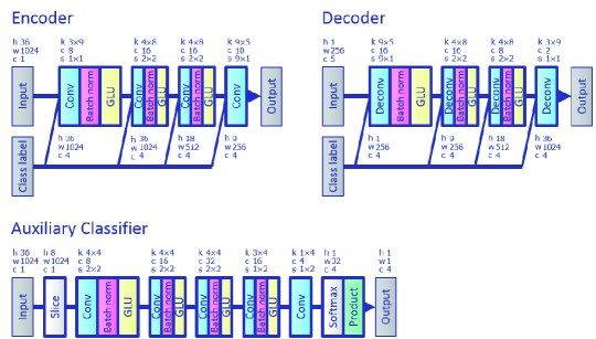
Fig. 2: Network architectures of the encoder, decoder and auxiliary classifier. Here, the input and output of each of the networks are interpreted as images, where “h”, “w” and “c” denote the height, width and channel number, respectively. “Conv”, “Batch norm”, “GLU”, “Deconv” “Softmax” and “Product” denote convolution, batch normalization, gated linear unit, transposed convolution, softmax, and product pooling layers, respectively. “k”, “c” and “s” denote the kernel size, output channel number and stride size of a convolution layer, respectively. Note that all the networks are fully convolutional with no fully connected layers, thus allowing inputs to have arbitrary sizes.

Encoder/Decoder: We use 2D CNNs to design the encoder and the decoder networks and the auxiliary classifier network by treating ${\bm{\mathbf{x}}}$ as an image of size $Q\times N$ with $1$ channel. Specifically, we use a gated CNN [37], which was originally introduced to model word sequences for language modeling and was shown to outperform long short-term memory (LSTM) language models trained in a similar setting. We previously employed gated CNN architectures for voice conversion [7, 38, 33] and monaural audio source separation [39], and their effectiveness has already been confirmed. In the encoder, the output of the $l$-th hidden layer, $\bm{\mathsf{h}}_{l}$, is described as a linear projection modulated by an output gate

$$\bm{\mathsf{h}}_{l-1}^{\prime} =[\bm{\mathsf{h}}_{l-1};\bm{\mathbf{c}}_{l-1}],$$ (16)

$$\bm{\mathsf{h}}_{l} =(\bm{\mathsf{W}}_{l}*\bm{\mathsf{h}}_{l-1}^{\prime}+\bm{\mathsf{b}}_{l})\odot\sigma(\bm{\mathsf{V}}_{l}*\bm{\mathsf{h}}_{l-1}^{\prime}+\bm{\mathsf{d}}_{l}),$$ (17)

where $\bm{\mathsf{W}}_{l}\in\mathbb{R}^{D_{l}\!\times\!D_{l-1}\!\times\!Q_{l}\!\times\!N_{l}}$, $\bm{\mathsf{b}}_{l}\in\mathbb{R}^{D_{l}}$, $\bm{\mathsf{V}}_{l}\in\mathbb{R}^{D_{l}\!\times\!D_{l-1}\!\times\!Q_{l}\!\times\!N_{l}}$ and $\bm{\mathsf{d}}_{l}\in\mathbb{R}^{D_{l}}$ are the encoder network parameters $\phi$, and $\sigma$ denotes the elementwise sigmoid function. Similar to LSTMs, the output gate multiplies each element of $\bm{\mathsf{W}}_{l}*\bm{\mathsf{h}}_{l-1}+\bm{\mathsf{b}}_{l}$ and control what information should be propagated through the hierarchy of layers. This gating mechanism is called a gated linear unit (GLU). Here, $[\bm{\mathsf{h}}_{l};\bm{\mathbf{c}}_{l}]$ means the concatenation of $\bm{\mathsf{h}}_{l}$ and $\bm{\mathbf{c}}_{l}$ along the channel dimension, and $\bm{\mathbf{c}}_{l}$ is a 3D array consisting of a $Q_{l}$-by-$N_{l}$ tiling of copies of $c$ in the time dimensions. The input into the 1st layer of the encoder is $\bm{\mathsf{h}}_{0}={\bm{\mathbf{x}}}$. The outputs of the final layer are given as regular linear projections

$${\bm{\mu}}_{\phi} =\bm{\mathsf{W}}_{L}*\bm{\mathsf{h}}_{L-1}^{\prime}+\bm{\mathsf{b}}_{L},$$ (18)

$$\log{\bm{\sigma}}_{\phi}^{2} =\bm{\mathsf{V}}_{L}*\bm{\mathsf{h}}_{L-1}^{\prime}+\bm{\mathsf{d}}_{L}.$$ (19)

The decoder network is constructed as described below:

$$\bm{\mathsf{h}}_{0} =\bm{\mathbf{z}},$$

$$\bm{\mathsf{h}}^{\prime}_{l-1} =[\bm{\mathsf{h}}_{l-1};\bm{\mathbf{c}}_{l-1}],$$

$$\bm{\mathsf{h}}_{l} =(\bm{\mathsf{W}}^{\prime}_{l}*\bm{\mathsf{h}}^{\prime}_{l-1}+\bm{\mathsf{b}}^{\prime}_{l})\odot\sigma(\bm{\mathsf{V}}^{\prime}_{l}*\bm{\mathsf{h}}^{\prime}_{l-1}+\bm{\mathsf{d}}^{\prime}_{l}),$$

$${\bm{\mu}}_{\theta} =\bm{\mathsf{W}}^{\prime}_{L}*\bm{\mathsf{h}}^{\prime}_{L-1}+\bm{\mathsf{b}}^{\prime}_{L},$$

$$\log{\bm{\sigma}}_{\theta}^{2} =\bm{\mathsf{V}}^{\prime}_{L}*\bm{\mathsf{h}}^{\prime}_{L-1}+\bm{\mathsf{d}}^{\prime}_{L},$$

where $\bm{\mathsf{W}}^{\prime}_{l}\in\mathbb{R}^{D_{l}\!\times\!D_{l-1}\!\times\!Q_{l}\times\!N_{l}}$, $\bm{\mathsf{b}}^{\prime}_{l}\in\mathbb{R}^{D_{l}}$, $\bm{\mathsf{V}}^{\prime}_{l}\in\mathbb{R}^{D_{l}\!\times\!D_{l-1}\!\times\!Q_{l}\!\times N_{l}}$ and $\bm{\mathsf{d}}^{\prime}_{l}\in\mathbb{R}^{D_{l}}$ are the decoder network parameters $\theta$. See Section 4 for more details. It should be noted that since the entire architecture is fully convolutional with no fully-connected layers, it can take an entire sequence with an arbitrary length as an input and generate an acoustic feature sequence of the same length.

Auxiliary Classifier: We also design an auxiliary classifier using a gated CNN, which takes an acoustic feature sequence $\bm{\mathbf{x}}$ and produces a sequence of class probability distributions that shows how likely each segment of $\bm{\mathbf{x}}$ is to belong to attribute $c$. The output of the $l$-th layer of the classifier is given as

$$\bm{\mathsf{h}}_{l} =(\bm{\mathsf{W}}^{\prime\prime}_{l}*\bm{\mathsf{h}}_{l-1}+\bm{\mathsf{b}}^{\prime\prime}_{l})\odot\sigma(\bm{\mathsf{V}}^{\prime\prime}_{l}*\bm{\mathsf{h}}_{l-1}+\bm{\mathsf{d}}^{\prime\prime}_{l}),$$ (20)

where $\bm{\mathsf{W}}^{\prime\prime}_{l}\in\mathbb{R}^{D_{l}\!\times\!D_{l-1}\!\times\!Q_{l}\times\!N_{l}}$, $\bm{\mathsf{b}}^{\prime\prime}_{l}\in\mathbb{R}^{D_{l}}$, $\bm{\mathsf{V}}^{\prime\prime}_{l}\in\mathbb{R}^{D_{l}\!\times\!D_{l-1}\!\times\!Q_{l}\!\times N_{l}}$ and $\bm{\mathsf{d}}^{\prime\prime}_{l}\in\mathbb{R}^{D_{l}}$ are the auxiliary classifier network parameters $\psi$. The final output $r_{\psi}(c|\bm{\mathbf{x}})$ is given by the product of all the elements of $\bm{\mathsf{h}}_{L}$. See Section 4 for more details.

4 Experiments

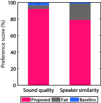
Fig. 3: Results of the AB test for sound quality and the ABX test for speaker similarity.

To confirm the performance of our proposed method, we conducted subjective evaluation experiments involving a non-parallel many-to-many speaker identity conversion task. We used the Voice Conversion Challenge (VCC) 2018 dataset [40], which consists of recordings of six female and six male US English speakers. We used a subset of speakers for training and evaluation. Specifically, we selected two female speakers, ‘VCC2SF1’ and ‘VCC2SF2’, and two male speakers, ‘VCC2SM1’ and ‘VCC2SM2’. Thus, $c$ is represented as a four-dimensional one-hot vector and in total there were twelve different combinations of source and target speakers. The audio files for each speaker were manually segmented into 116 short sentences (each about 7 minutes long) where 81 and 35 sentences (each, respectively, about 5 and 2 minutes long) were provided as training and evaluation sets, respectively. All the speech signals were sampled at 22050 Hz. For each utterance, a spectral envelope, a logarithmic fundamental frequency (log $F_{0}$), and aperiodicities (APs) were extracted every 5 ms using the WORLD analyzer [35]. 36 mel-cepstral coefficients (MCCs) were then extracted from each spectral envelope. The $F_{0}$ contours were converted using the logarithm Gaussian normalized transformation described in [41]. The aperiodicities were used directly without modification. The network configuration is shown in detail in Fig. 2. The signals of the converted speech were obtained using the method described in 3.3.

We chose the VAEGAN-based approach [19] for comparison with our experiments. Although we would have liked to replicate the implementation of this method exactly, we made our own design choices because certain details of the network configuration and hyperparameters were missing. We conducted an AB test to compare the sound quality of the converted speech samples and an ABX test to compare the similarity to the target speaker of the converted speech samples, where “A” and “B” were converted speech samples obtained with the proposed and baseline methods and “X” was a real speech sample obtained from a target speaker. With these listening tests, “A” and “B” were presented in random orders to eliminate bias in the order of stimuli. Eight listeners participated in our listening tests. For the AB test of sound quality, each listener was presented {“A”,“B”} $\times$ 20 utterances, and for the ABX test of speaker similarity, each listener was presented {“A”,“B”,“X”} $\times$ 24 utterances. Each listener was then asked to select “A”, “B” or “fair” for each utterance. The results are shown in Fig. 3. As the results reveal, the proposed method significantly outperformed the baseline method in terms of both sound quality and speaker similarity. Audio samples are provided at http://www.kecl.ntt.co.jp/people/kameoka.hirokazu/Demos/ acvae-vc/.

5 Conclusions

This paper proposed a non-parallel many-to-many VC method using a VAE variant called an auxiliary classifier VAE (ACVAE). The proposed method has three key features. First, we adopted fully convolutional architectures to construct the encoder and decoder networks so that the networks could learn conversion rules that capture time dependencies in the acoustic feature sequences of source and target speech. Second, we proposed using an information-theoretic regularization for the model training to ensure that the information in the latent attribute label would not be lost in the generation process. With regular CVAEs, the encoder and decoder are free to ignore the attribute class label input. This can be problematic since in such a situation, the attribute class label input will have little effect on controlling the voice characteristics of the input speech. To avoid such situations, we proposed introducing an auxiliary classifier and training the encoder and decoder so that the attribute classes of the decoder outputs are correctly predicted by the classifier. Third, to avoid producing buzzy-sounding speech at test time, we proposed simply transplanting the spectral details of the input speech into its converted version. Subjective evaluation experiments on a non-parallel many-to-many speaker identity conversion task revealed that the proposed method obtained higher sound quality and speaker similarity than the VAEGAN-based method.

References

- [1] A. Kain and M. W. Macon, “Spectral voice conversion for text-to-speech synthesis,” in Proc. ICASSP, 1998, pp. 285–288.
- [2] A. B. Kain, J.-P. Hosom, X. Niu, J. P. van Santen, M. Fried-Oken, and J. Staehely, “Improving the intelligibility of dysarthric speech,” Speech Commun., vol. 49, no. 9, pp. 743–759, 2007.
- [3] K. Nakamura, T. Toda, H. Saruwatari, and K. Shikano, “Speaking-aid systems using GMM-based voice conversion for electrolaryngeal speech,” Speech Commun., vol. 54, no. 1, pp. 134–146, 2012.
- [4] Z. Inanoglu and S. Young, “Data-driven emotion conversion in spoken English,” Speech Commun., vol. 51, no. 3, pp. 268–283, 2009.
- [5] O. Türk and M. Schröder, “Evaluation of expressive speech synthesis with voice conversion and copy resynthesis techniques,” IEEE/ACM Trans. Audio Speech Lang. Process., vol. 18, no. 5, pp. 965–973, 2010.
- [6] T. Toda, M. Nakagiri, and K. Shikano, “Statistical voice conversion techniques for body-conducted unvoiced speech enhancement,” IEEE/ACM Trans. Audio Speech Lang. Process., vol. 20, no. 9, pp. 2505–2517, 2012.
- [7] T. Kaneko, H. Kameoka, K. Hiramatsu, and K. Kashino, “Sequence-to-sequence voice conversion with similarity metric learned using generative adversarial networks,” in Proc. Interspeech, 2017, pp. 1283–1287.
- [8] Y. Stylianou, O. Cappé, and E. Moulines, “Continuous probabilistic transform for voice conversion,” IEEE Trans. Speech and Audio Process., vol. 6, no. 2, pp. 131–142, 1998.
- [9] T. Toda, A. W. Black, and K. Tokuda, “Voice conversion based on maximumlikelihood estimation of spectral parameter trajectory,” IEEE/ACM Trans. Audio Speech Lang. Process., vol. 15, no. 8, pp. 2222–2235, 2007.
- [10] E. Helander, T. Virtanen, J. Nurminen, and M. Gabbouj, “Voice conversion using partial least squares regression,” IEEE/ACM Trans. Audio Speech Lang. Process., vol. 18, no. 5, pp. 912–921, 2010.
- [11] L.-H. Chen, Z.-H. Ling, L.-J. Liu, and L.-R. Dai, “Voice conversion using deep neural networks with layer-wise generative training,” IEEE/ACM Trans. Audio Speech Lang. Process., vol. 22, no. 12, pp. 1859–1872, 2014.
- [12] T. Nakashika, T. Takiguchi, and Y. Ariki, “Voice conversion based on speaker-dependent restricted Boltzmann machines,” IEICE Trans. Inf. Syst., vol. 97, no. 6, pp. 1403–1410, 2014.
- [13] S. Desai, A. W. Black, B. Yegnanarayana, and K. Prahallad, “Spectral mapping using artificial neural networks for voice conversion,” IEEE/ACM Trans. Audio Speech Lang. Process., vol. 18, no. 5, pp. 954–964, 2010.
- [14] S. H. Mohammadi and A. Kain, “Voice conversion using deep neural networks with speaker-independent pre-training,” in Proc. SLT, 2014, pp. 19–23.
- [15] T. Nakashika, T. Takiguchi, and Y. Ariki, “High-order sequence modeling using speaker-dependent recurrent temporal restricted boltzmann machines for voice conversion,” in Proc. Interspeech, 2014, pp. 2278–2282.
- [16] L. Sun, S. Kang, K. Li, and H. Meng, “Voice conversion using deep bidirectional long short-term memory based recurrent neural networks,” in Proc. ICASSP, 2015, pp. 4869–4873.
- [17] M. Blaauw and J. Bonada, “Modeling and transforming speech using variational autoencoders,” in Proc. Interspeech, 2016, pp. 1770–1774.
- [18] C.-C. Hsu, H.-T. Hwang, Y.-C. Wu, Y. Tsao, and H.-M. Wang, “Voice conversion from non-parallel corpora using variational auto-encoder,” in Proc. APSIPA, 2016, pp. 1–6.
- [19] C.-C. Hsu, H.-T. Hwang, Y.-C. Wu, Y. Tsao, and H.-M. Wang, “Voice conversion from unaligned corpora using variational autoencoding Wasserstein generative adversarial networks,” in Proc. Interspeech, 2017, pp. 3364–3368.
- [20] R. Takashima, T. Takiguchi, and Y. Ariki, “Exampler-based voice conversion using sparse representation in noisy environments,” IEICE Trans. Inf. Syst., vol. E96-A, no. 10, pp. 1946–1953, 2013.
- [21] Z. Wu, T. Virtanen, E. S. Chng, and H. Li, “Exemplar-based sparse representation with residual compensation for voice conversion,” IEEE/ACM Trans. Audio Speech Lang. Process., vol. 22, no. 10, pp. 1506–1521, 2014.
- [22] F.-L. Xie, F. K. Soong, and H. Li, “A KL divergence and DNN-based approach to voice conversion without parallel training sentences,” in Proc. Interspeech, 2016, pp. 287–291.
- [23] T. Kinnunen, L. Juvela, P. Alku, and J. Yamagishi, “Non-parallel voice conversion using i-vector PLDA: Towards unifying speaker verification and transformation,” in Proc. ICASSP, 2017, pp. 5535–5539.
- [24] N. Dehak, P. Kenny, R. Dehak, P. Dumouchel, and P. Ouellet, “Front-end factor analysis for speaker verification,” IEEE. Trans. Audio Speech Lang. Process., vol. 19, no. 4, pp. 788–798, 2011.
- [25] D. P. Kingma and M. Welling, “Auto-encoding variational Bayes,” in Proc. ICLR, 2014.
- [26] D. P. Kingma and D. J. Rezendey, S. Mohamedy, and M. Welling, “Semi-supervised learning with deep generative models,” in Adv. Neural Information Processing Systems (NIPS), 2014, pp. 3581–3589.
- [27] Y. Saito, Y. Ijima, K. Nishida, and S. Takamichi, “Non-parallel voice conversion using variational autoencoders conditioned by phonetic posteriorgrams and d-vectors,” in Proc. ICASSP, 2018, pp. 5274–5278.
- [28] A. B. L. Larsen, S. K. Sønderby, H. Larochelle, and O. Winther, “Autoencoding beyond pixels using a learned similarity metric,” arXiv:1512.09300 [cs.LG], Dec. 2015.
- [29] X. Chen, Y. Duan, R. Houthooft, J. Schulman, I. Sutskever, and P. Abbeel, “InfoGAN: Interpretable representation learning by information maximizing generative adversarial nets,” in Proc. NIPS, 2016.
- [30] D. Barber and F. V. Agakov, “The IM algorithm: A variational approach to information maximization,” in Proc. NIPS, 2003.
- [31] A. Odena, C. Olah, and J. Shlens, “Conditional image synthesis with auxiliary classifier GANs,” in Proc. ICML, 2017, vol. PMLR 70, pp. 2642–2651.
- [32] Y. Choi, M. Choi, M. Kim, J.-W. Ha, S. Kim, and J. Choo, “StarGAN: Unified generative adversarial networks for multi-domain image-to-image translation,” arXiv:1711.09020 [cs.CV], Nov. 2017.
- [33] H. Kameoka, T. Kaneko, K. Tanaka, and N. Hojo, “StarGAN-VC: Non-parallel many-to-many voice conversion with star generative adversarial networks,” arXiv:1806.02169 [cs.SD], June 2018.
- [34] T. Fukada, K. Tokuda, T. Kobayashi, and S. Imai, “An adaptive algorithm for mel-cepstral analysis of speech,” in Proc. ICASSP, 1992, pp. 137–140.
- [35] M. Morise, F. Yokomori, and K. Ozawa, “WORLD: a vocoder-based high-quality speech synthesis system for real-time applications,” IEICE trans. Inf. Syst., vol. E99-D, no. 7, pp. 1877–1884, 2016.
- [36] K. Kobayashi, T. Toda, and S. Nakamura, “ transformation techniques for statistical voice conversion with direct waveform modification with spectral differential,” in Proc. SLT, 2016, pp. 693–700.
- [37] Y. N. Dauphin, A. Fan, M. Auli, and D. Grangier, “Language modeling with gated convolutional networks,” in Proc. ICML, 2017, pp. 933–941.
- [38] T. Kaneko and H. Kameoka, “Parallel-data-free voice conversion using cycle-consistent adversarial networks,” arXiv:1711.11293 [stat.ML], Nov. 2017.
- [39] L. Li and H. Kameoka, “Deep clustering with gated convolutional networks,” in Proc. ICASSP, 2018, pp. 16–20.
- [40] J. Lorenzo-Trueba, J. Yamagishi, T. Toda, D. Saito, F. Villavicencio, T. Kinnunen, and Z. Ling, “The voice conversion challenge 2018: Promoting development of parallel and nonparallel methods,” arXiv:1804.04262 [eess.AS], Apr. 2018.
- [41] K. Liu, J. Zhang, and Y. Yan, “High quality voice conversion through phoneme-based linear mapping functions with STRAIGHT for mandarin,” in Proc. FSKD, 2007, pp. 410–414.