The Steady-State Behavior of Multivariate Exponentially Weighted Moving Average Control Charts

Abstract.

Multivariate Exponentially Weighted Moving Average, MEWMA, charts are popular, handy and effective procedures to detect distributional changes in a stream of multivariate data. For doing appropriate performance analysis, dealing with the steady-state behavior of the MEWMA statistic is essential. Going beyond early papers, we derive quite accurate approximations of the respective steady-state densities of the MEWMA statistic. It turns out that these densities could be rewritten as the product of two functions depending on one argument only which allows feasible calculation. For proving the related statements, the presentation of the non-central chisquare density deploying the confluent hypergeometric limit function is applied. Using the new methods it was found that for large dimensions, the steady-state behavior becomes different to what one might expect from the univariate monitoring field. Based on the integral equation driven methods, steady-state and worst-case average run lengths are calculated with higher accuracy than before. Eventually, optimal MEWMA smoothing constants are derived for all considered measures.

1. Introduction

Multivariate monitoring tasks result often in some type of Multivariate Exponentially Weighted Moving Average (MEWMA) which was introduced by Lowry et al., (1992) as extension of the even more popular $T^{2}$ chart proposed initially by Hotelling, (1947). Refer to Yang et al., (2018) and Harrou et al., (2018) for recent applications of MEWMA in the field of fault detection in wind turbines and photovoltaic systems, respectively. In a nutshell, MEWMA charts aim to detecting changes in the distribution (here in the mean) of multivariate data as quickly as possible while maintaining a reasonable level of false alarms. The most common operating characteristic of a monitoring device alias control chart is the Average Run Length (ARL) introduced already in Page, (1954). Its typical appearance is often called zero-state ARL and refers to the situation that the state of the control chart at the time of change is known. To describe this more thoroughly, we take a look at our data model. Here we consider a sequence of serially independent normally distributed vectors $\bm{X}_{1},\bm{X}_{2},\ldots$ of dimension $p$, that is

$$\bm{X}_{n}\sim\mathcal{N}(\bm{\mu},\Sigma)\;\;,\;n=1,2,\ldots$$

To avoid further complications, we assume that the covariance matrix $\Sigma$ is known, and the mean vector $\bm{\mu}$ follows the simple change point model: $\bm{\mu}=\bm{\mu}_{0}$ for $n<\tau$, and $\bm{\mu}=\bm{\mu}_{1}$ for $n\geq\tau$. The change point $\tau$ is, of course, unknown, while $\bm{\mu}_{0}$ is given (either by knowing the process or by estimating during a preliminary study). The other mean value, $\bm{\mu}_{1}$, induces certain choices of control chart parameters. Following Lowry et al., (1992), the MEWMA sequence $\{\bm{Z}_{n}\}$ is formed by

(1) $$\bm{Z}_{0}=\bm{z}_{0}\;,\;\;\bm{Z}_{n}=(1-\lambda)\bm{Z}_{n-1}+\lambda\bm{X}_{n}\quad,\;n=1,2,\ldots\;,\;\;0<\lambda\leq 1\,.$$

In parallel, we determine the Mahalanobis distance $T_{n}^{2}=(\bm{Z}_{n}-\bm{\mu}_{0})^{\prime}\Sigma_{Z}^{-1}(\bm{Z}_{n}-\bm{\mu}_{0})$ from the stable mean $\bm{\mu}_{0}$, where $\Sigma_{Z}$ denotes the asymptotic covariance matrix of $\bm{Z}_{n}$ with

$$\Sigma_{Z}=\lim_{n\to\infty}Cov(\bm{Z}_{n})=\frac{\lambda}{2-\lambda}\Sigma\,.$$

If this distance, $T_{n}^{2}$, becomes larger than a given threshold $h_{4}$ (naming convention stems from Lowry et al.,, 1992), an alarm is triggered which is linked to the MEWMA stopping time

(2) $$N=\inf\big{\{}n\geq 1:T_{n}^{2}>h_{4}\big{\}}\,.$$

Its expected value for two exemplary cases, $\tau=1$ or $\tau=\infty$, is just the aforementioned zero-state average run length (ARL), roughly speaking. In the sequel, this is written as $E_{\infty}(N)$ (in-control case) and $E_{1}(N)$ (out-of-control case) with the general expression $E_{\tau}()$ denoting the expectation for given change point $\tau$. In order to obtain actual numbers, Lowry et al., (1992) deployed Monte Carlo simulations, Rigdon, 1995a ; Rigdon, 1995b provided numerical solutions of ARL integral equations, and Runger and Prabhu, (1996) presented a Markov chain approximation. Recently, Knoth, (2017) demonstrated some accuracy problems of these algorithms and offered improved numerical solutions of Rigdon, 1995a ; Rigdon, 1995b . However, only the Monte Carlo and the Markov chain approach are expanded to determine the steady-state ARL, which measures the average number of observations until signal after the change point $\tau$, while assuming that the sequence $\bm{Z}_{n}$ reached its steady state before $\tau$. Namely, Prabhu and Runger, (1997) utilized the Markov chain model to calculate the steady-state ARL. Their algorithm was used, for example, in Lee and Khoo, (2014). However, its deployment is complicated and, differently to the zero-state ARL, no software implementation is published. Hence, others used Monte Carlo studies, see, for example, Reynolds Jr. and Stoumbos, (2008) and Zou and Tsung, (2011). Before we start to investigate the steady-state ARL in more detail, we want to emphasize its importance as performance indicator of a monitoring device. Because the actual position of the change point $\tau$ is unknown, we do not know neither the position of the MEWMA statistic $\bm{Z}_{\tau-1}$ nor its distance to $\bm{\mu}_{0}$, $T_{\tau-1}^{2}$, one observation before the change occurs. For the mentioned zero-state ARL we imply that $\bm{Z}_{\tau-1}=\bm{\mu}_{0}$ and $T_{\tau-1}^{2}=0$, respectively, what might be substantially misleading. More appropriate would be to exploit the steady-state behavior of $\bm{Z}_{\tau-1}$ in order to weight in a reasonable way possible positions of $\bm{Z}_{\tau-1}$ and the resulting detection delay $\sim N-\tau$. More conservative would be to investigate the worst-case position of $\bm{Z}_{\tau-1}$. Both ways will be treated and finally compared to the classic Hotelling-Shewhart chart which remained popular for monitoring users being afraid of inertia problems which often escort the application of (M)EWMA. Fortunately, Rigdon, 1995a indicated that it suffices to study the simple case $\bm{\mu}_{0}=\bm{0}$ and $\Sigma=\mathbb{I}$ (identity matrix) by only assuming that the original covariance matrix $\Sigma$ is positive definite. Hence, in the sequel we set both terms accordingly.

The paper is organized as follows: In Section 2 the concepts of steady-state ARL are described in more detail while evaluating the in-control case. The more involved and much more important out-of-control case is examined in Section 3. In the subsequent Section 4 the framework is applied to illustrate the detection performance of MEWMA using the zero-state, steady-state and worst-case ARL. Eventually, the conclusions section completes the paper. Proofs and similar technical details are collected in the Appendix.

2. Steady-state methodology and the in-control case

Measuring the detection delay after reaching some steady state was already utilized in Roberts, (1966). Beginning with Taylor, (1968) and later on with Yashchin, (1985) and Crosier, (1986), the concepts were consolidated. Using the naming conventions of Crosier, (1986), two different types of steady-state ARL are defined in the following way. The first and presumably more popular one assumes that no (false) alarm is raised before the change takes place. It is called conditional steady-state ARL and could be written as

(3) $$\mathcal{D}=\lim\limits_{\tau\to\infty}E_{\tau}\big{(}N-\tau+1\mid N\geq\tau\big{)}\,.$$

The second one refers to the situation that the change happens after a sequence of false alarms. The control chart is re-started after each of them so that the cyclical steady-state ARL could be expressed by

(4) $$\mathcal{D}_{\star} =\lim\limits_{\tau\to\infty}E_{\tau}\big{(}N_{\star}-\tau+1)\,,$$

$$N_{\star} =N_{1}+N_{2}+\ldots+N_{I_{\tau}-1}+N_{I_{\tau}}\;,\,I_{\tau}=\min\left\{i\geq 1:\sum_{j=1}^{i}N_{j}\geq\tau\right\}.$$

See Pollak and Tartakovsky, (2009), Section 3, for a more rigor treatment of $\mathcal{D}_{\star}$ and asymptotic optimality in the univariate case. Both steady-state ARL types are calculated by combining the (quasi-)stationary distribution of the control chart statistic and the ARL as function of the actual value of the latter statistic. To develop our approach, we start with the simpler in-control case, where it is sufficient to consider for both functions only one argument, the distance $T_{n}^{2}$. Recall the ARL integral equation of Rigdon, 1995a with $\alpha=\bm{z}_{0}^{\prime}\bm{z_{0}}$ being the distance of the initial $\bm{Z}_{0}$ value to zero in (1):

(5) $$\mathcal{\mathring{L}}(\alpha)=1+\int_{0}^{h}\mathcal{\mathring{L}}(u)\frac{1}{\lambda^{2}}f_{\chi^{2}}\left(\frac{u}{\lambda^{2}}\,\Big{|}\,p,\left[\frac{1-\lambda}{\lambda}\right]^{2}\!\!\alpha\right)\mathrm{d}u\,,$$

where $\mathcal{\mathring{L}}(\alpha)=E_{\infty}(N)$ for $\bm{Z}_{0}=\bm{z}_{0}$ (the superscript $\mathring{\,}$ marks the in-control case) and $h=h_{4}\lambda/(2-\lambda)$. The function $f_{\chi^{2}}(\cdot\mid p,\nu)$ denotes the probability density of the non-central $\chi^{2}$ distribution with $p$ degrees of freedom and noncentrality parameter $\nu=\eta\alpha=\left[\frac{1-\lambda}{\lambda}\right]^{2}\!\!\alpha$. Rigdon, 1995a solved (5) numerically by applying the Nyström method (Nyström,, 1930) with Gauß-Radau quadrature. Recently, Knoth, (2017) utilized the slightly more powerful Gauß-Legendre quadrature after a change in variables from $\alpha$ to $\alpha^{2}$ which improves the accuracy for odd $p$ substantially. A similar integral equation is valid for the left eigenfunction $\mathring{\psi}()$, the quasi-stationary density of $Z_{\tau-1}$, which is needed for the conditional steady-state ARL $\mathcal{D}$:

(6) $$\varrho\mathring{\psi}(u)=\int_{0}^{h}\mathring{\psi}(\alpha)\frac{1}{\lambda^{2}}f_{\chi^{2}}\left(\frac{u}{\lambda^{2}}\,\Big{|}\,p,\eta\alpha\right)\mathrm{d}\alpha\,.$$

Refer to Knoth, (2016) for more details about the family of integral equations to calculate the ARL function $\mathcal{\mathring{L}}()$ and the left eigenfunction $\mathring{\psi}()$ in case of univariate EWMA charts. A similar list is given in Moustakides et al., (2009) for CUSUM and Shiryaev-Roberts schemes. The parameter $\varrho$ is just the dominating eigenvalue of the integral kernel in (6) which provides essential information about the long running behavior of the MEWMA stopping time $N$ in the in-control case — $P_{\infty}(N=n\mid N\geq n)\approx 1-\varrho$ for large $n$ (classical paper is, for example, Gold,, 1989). Applying the same change in variables as performed in Knoth, (2017) for (5), one obtains

(7) $$\varrho\mathring{\psi}_{i}=\sum_{j=1}^{r}w_{j}\mathring{\psi}_{j}\frac{1}{\lambda^{2}}f_{\chi^{2}}\left(\frac{z_{i}^{2}}{\lambda^{2}}\,\Big{|}\,p,\eta z_{j}^{2}\right)2z_{j}\qquad\text{ with }\mathring{\psi}_{i}=\mathring{\psi}(z_{i}^{2})\,,$$

where $w_{j}$ and $z_{j}$ are the weights and nodes of the Gauß-Legendre quadrature. The system (7) could be solved either by the power method (von Mises and Pollaczek-Geiringer,, 1929) or by applying readily available routines such as eigen() in the statistics software system R which calls eventually well established procedures from the BLAS (Lawson et al.,, 1979) or LAPACK (Anderson et al.,, 1999) libraries (more information on http://www.netlib.org). Collecting the numerical solutions of (5) and (7) in matrices and vectors we can write

$$\bm{\mathring{\ell}}=(\mathbb{I}-\mathbb{Q}_{\mathcal{L}})^{-1}\bm{1}\quad\text{ and }\quad\varrho\bm{\mathring{\psi}}=\mathbb{Q}_{\psi}\bm{\mathring{\psi}}\,,\\$$

and obtain

$$\mathring{\mathcal{D}}=\frac{(\mathbb{W}\bm{\mathring{\psi}})^{\prime}\bm{\mathring{\ell}}}{(\mathbb{W}\bm{\mathring{\psi}})^{\prime}\bm{1}}\quad\text{ with }\quad\mathbb{W}=\mathop{\mathrm{diag}}(2w_{i}z_{i})$$

as numerical counterpart to (3). More details are given in the Appendix. Next, we derive the integral equation for the cyclical steady-state ARL according to (4). The now stationary density (linked to the eigenvalue $\varrho=1$) follows

(8) $$\mathring{\psi}_{\star}(u)=\Psi_{0}\frac{1}{\lambda^{2}}f_{\chi^{2}}\left(\frac{u}{\lambda^{2}}\,\Big{|}\,p\right)+\int_{0}^{h}\mathring{\psi}_{\star}(\alpha)\frac{1}{\lambda^{2}}f_{\chi^{2}}\left(\frac{u}{\lambda^{2}}\,\Big{|}\,p,\eta\alpha\right)\mathrm{d}\alpha\,,$$

which results after plugging in the Gauß-Legendre quadrature in a common linear equation system,

(9) $$\bm{\mathring{\psi}}_{\star}=(\mathbb{I}-\mathbb{Q}_{\psi})^{-1}\bm{f}\quad\text{ and }\quad\bm{f}=(f_{1},\ldots,f_{r})^{\prime}\;,\;\;f_{i}=\frac{\Psi_{0}}{\lambda^{2}}f_{\chi^{2}}\left(\frac{z_{i}^{2}}{\lambda^{2}}\,\Big{|}\,p\right)\,.$$

The additional parameter $\Psi_{0}$ labels the probability of $\bm{Z}_{\tau-1}=\bm{z}_{0}=\bm{0}$ for $\tau\to\infty$ and equals to $1/E_{\infty}(N)$ because the restart in $\bm{z}_{0}$ is a renewal point, cf. Knoth, (2016) for more details. The solution in (9) complies $(\mathbb{W}\bm{\mathring{\psi}}_{\star})^{\prime}\bm{1}+\Psi_{0}=1$ by construction so that we can write

$$\mathring{\mathcal{D}}_{\star}=\Psi_{0}\,\mathcal{\mathring{L}}(0)+(\mathbb{W}\bm{\mathring{\psi}}_{\star})^{\prime}\bm{\ell}$$

as numerical approximation of the cyclical steady-state ARL. Note that being in the in-control case, we receive $\Psi_{0}\,\mathcal{\mathring{L}}(0)=1$, because $\mathcal{\mathring{L}}(0)=E_{\infty}(N)$. In the here following Figure 1 we illustrate the shape of $\mathring{\psi}()$ and $\mathring{\psi}_{\star}()$ for dimensions $p\in\{2,3,4,10\}$ and $E_{\infty}(N)=200$.

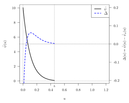
(a) $p=2$

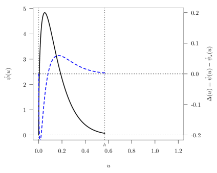
(b) $p=3$

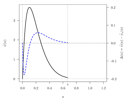
(c) $p=4$

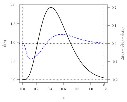
(d) $p=10$

Figure 1. Left eigenfunctions, $\mathring{\psi}()$ and $\mathring{\psi}_{\star}()$ (actually, $\Delta()=\mathring{\psi}()-\mathring{\psi}_{\star}()$ is plotted), needed to calculate both steady-state ARL types, $\mathring{\mathcal{D}}$ and $\mathring{\mathcal{D}}_{\star}$, in the in-control case for selected dimensions $p$, smoothing constant $\lambda=0.1$, and $E_{\infty}(N)=200$.

Because the differences between $\mathring{\psi}()$ and $\mathring{\psi}_{\star}()$ are quite small, we plot $\mathring{\psi}()$ and $\Delta()=\mathring{\psi}()-\mathring{\psi}_{\star}()$. The corresponding thresholds for $\lambda=0.1$ are $h_{4}\in\{8.63,10.78,12.72,22.66\}$. The smallest dimension, $p=2$, yields a special shape of $\mathring{\psi}()$ which looks similar to an exponential distribution, while for all other $p$ we observe $\mathring{\psi}(0)=0$ and a pronounced mode at $u>0$ which increases with $p$. Because the re-start for the cyclical case takes place at $\bm{z}_{0}=\bm{0}$ yielding $u=0$, $\mathring{\psi}_{\star}(u)$ is larger than $\mathring{\psi}(u)$ for small $u$. For larger values of $u$, $\mathring{\psi}(u)$ is mildly larger than $\mathring{\psi}_{\star}(u)$. Note that the area under $\mathring{\psi}()$ is equal to 1, while it is $1-\Psi_{0}=0.995$ for $\mathring{\psi}_{\star}()$, because of the atom at $u=0$. The latter is the steady-state probability of $\bm{Z}_{\tau-1}=\bm{0}$ which is equal to $\Psi_{0}=1/200$. In addition, we provide some numerical results for $\mathring{\mathcal{D}}$ and $\mathring{\mathcal{D}}_{\star}$ for different $\lambda$ and $p$ in Table 1.

Table 1. In-control steady-state ARL results for various $p$, smoothing constants $\lambda\in\{0.05,0.1,0.2\}$, and $E_{\infty}(N)=200$.

	$p$
ARL	2	3	4	5	10	20	50
$\lambda=0.05$
$\mathring{\mathcal{D}}$	187.0	185.5	184.4	183.5	180.8	178.0	174.1
$\mathring{\mathcal{D}}_{\star}$	187.6	186.2	185.2	184.4	181.9	179.4	176.0
$\lambda=0.1$
$\mathring{\mathcal{D}}$	192.6	191.8	191.3	190.9	189.6	188.3	186.4
$\mathring{\mathcal{D}}_{\star}$	192.7	192.1	191.6	191.2	190.0	188.7	186.9
$\lambda=0.2$
$\mathring{\mathcal{D}}$	196.1	195.8	195.6	195.4	194.8	194.2	193.3
$\mathring{\mathcal{D}}_{\star}$	196.2	195.9	195.7	195.5	194.9	194.3	193.5

We notice that the steady-state ARL gets closer to the zero-state ARL for increasing $\lambda$. Moreover, the differences between $\mathring{\mathcal{D}}$ and $\mathring{\mathcal{D}}_{\star}$ vanish simultaneously. On the other hand, for increasing dimension $p$, the steady-state ARL decreases. Closing this section, we want to note two points. First, both types of the in-control steady-state ARL could be understood as expected number of observations until a false signal, told to a person (either the control chart owner or just a “witness”) who checks the state of a MEWMA chart on an arbitrary day knowing only that “no alarm occurred so far” (conditional) or “only false alarms occurred” (cyclical). Second, Prabhu and Runger, (1997) reported in their Table 3 (rows with $\delta=0$) corresponding numbers that are surprisingly close to 200, the zero-state value. The Monte Carlo studies we performed in Section 4 confirm essentially our numbers. In the next section we turn to the more involved out-of-control case.

3. Analysis of the out-of-control case

First, we recall the framework of Prabhu and Runger, (1997). They claimed to “provide conditional steady-state ARLs in Table 3.” In order to do this, they took the transition matrix $\mathbb{P}_{0}$ (counterpart to our matrix $\mathbb{Q}_{\mathcal{L}}$, but $\mathbb{P}_{0}$ refers to a bivariate Markov chain), calculated $\bm{v}^{\prime}=\bm{b}^{\prime}(\mathbb{I}-\mathbb{P}_{0})^{-1}$ and created by $\bm{q}=\bm{v}/(\bm{v}^{\prime}\bm{1})$ the needed steady-state distribution. Remind that the vector $\bm{b}$ consists of only zeros except for the component that corresponds to the starting state ($\bm{z}_{0}$), which is set to 1. Following Darroch and Seneta, (1965), Prabhu and Runger, (1997) rather determined the cyclical steady-state distribution, and consequently $\mathcal{D}_{\star}$. Later on, we will see that this is, of course, mathematically important, but in terms of actual numbers less relevant. Here we calculate both types, $\mathcal{D}$ and $\mathcal{D}_{\star}$, while connecting them carefully to their theoretical origins. In addition, we propose an algorithm which avoids the problem of dealing with such large matrices like $\mathbb{P}_{0}$ which stems from a bivariate Markov chain.

Contrary to Prabhu and Runger, (1997), we start from the (double) integral equation developed in Rigdon, 1995b for the out-of-control zero-state ARL, which is a function of two arguments. Besides the already introduced $\alpha=\bm{z}_{0}^{\prime}\bm{z}_{0}$ we utilize as second argument $\beta=\bm{\mu}_{1}^{\prime}\bm{z}_{0}$. Recall also the value $\delta=\bm{\mu}_{1}^{\prime}\bm{\mu}_{1}$ which quantifies the magnitude of the change. From Rigdon, 1995b we present for the out-of-control zero-state ARL ($\alpha\in[0,h]$, $\beta^{2}\leq\alpha\delta$)

$$\mathcal{L}(\alpha,\beta) =1+\int_{-\sqrt{\delta h}}^{\sqrt{\delta h}}\int_{v^{2}/\delta}^{h}\mathcal{L}(u,v)K(u,v;\alpha,\beta)\,\mathrm{d}u\,\mathrm{d}v\,,$$

$$K(u,v;\alpha,\beta) =\frac{1}{\sqrt{2\pi\delta\lambda^{2}}}e^{-\frac{[v-\lambda\delta-(1-\lambda)\beta]^{2}}{2\delta\lambda^{2}}}$$

$$\qquad\times\frac{1}{\lambda^{2}}f_{\chi^{2}}\left(\!\frac{u-v^{2}/\delta}{\lambda^{2}}\,\Big{|}\,p-1,\eta(\alpha-\beta^{2}/\delta)\!\right)\,.$$

Regarding the numerical solution of this double integral equation we refer to Rigdon, 1995b and Knoth, (2017). For preparing the left eigenfunction equation, we change the integration order and the second argument. Writing $\theta$ for the angle between the initial MEWMA value $\bm{z}_{0}$ and the new mean vector $\bm{\mu}_{1}$, we deduce $\beta=\sqrt{\alpha}\sqrt{\delta}\cos(\theta)$. The new second argument is set by $\gamma=-\cos(\theta)$ for convenience (more details see the Appendix) so that we get the following double integral equation:

(10) $$\mathcal{L}(\alpha,\gamma) =1+\int_{0}^{h}\int_{-1}^{1}\mathcal{L}(u,w)K^{\dagger}(u,w;\alpha,\gamma)\,\mathrm{d}w\,\mathrm{d}u\,,$$

$$K^{\dagger}(u,w;\alpha,\gamma) =\frac{\sqrt{u}}{\sqrt{2\pi\lambda^{2}}}e^{-\frac{[\sqrt{u}w-\lambda\sqrt{\delta}-(1-\lambda)\sqrt{\alpha}\gamma]^{2}}{2\lambda^{2}}}$$

$$\qquad\times\frac{1}{\lambda^{2}}f_{\chi^{2}}\left(\frac{u(1-w^{2})}{\lambda^{2}}\,\Big{|}\,p-1,\eta\alpha(1-\gamma^{2})\right)\,.$$

Studying (10) we conclude that we have to account for the (quasi-)stationary distributions of both the distance to zero, $\alpha$, and the angle $\theta$ ($\gamma=-\cos(\theta)$ links $\theta$ and $\gamma$) between the new mean $\bm{\mu}_{1}$ and the MEWMA statistic $\bm{Z}_{\tau-1}$. Similarly to the transition from $\mathcal{\mathring{L}}(\alpha)$ to $\mathring{\psi}(u)$ we derive the integral equation for $\psi(u,w)$,

(11) $$\varrho\psi(u,w)=\int_{0}^{h}\int_{-1}^{1}\psi(\alpha,\gamma)K^{\dagger}(u,w;\alpha,\gamma)\,\mathrm{d}\gamma\,\mathrm{d}\alpha\,,$$

and for the cyclical case (restart at $\bm{z_{0}}=\bm{0}$)

(12) $$\psi_{\star}(u,w)=\Psi_{0}K^{\dagger}(u,w;0,0)+\int_{0}^{h}\int_{-1}^{1}\psi_{\star}(\alpha,\gamma)K^{\dagger}(u,w;\alpha,\gamma)\,\mathrm{d}\gamma\,\mathrm{d}\alpha\,.$$

Because we evaluate both eigenfunction equations for the in-control parameter setup analogously to Prabhu and Runger, (1997), we set $\delta=0$ and simplify

$$K^{\dagger}(u,w;\alpha,\gamma) =\ldots e^{-\frac{[\sqrt{u}w-(1-\lambda)\sqrt{\alpha}\gamma]^{2}}{2\lambda^{2}}}\ldots\,,$$

$$K^{\dagger}(u,w;0,0) =\frac{\Gamma(\frac{p}{2})}{\Gamma(\frac{p-1}{2})\sqrt{\pi}}(1-w^{2})^{\frac{p-3}{2}}\times\frac{1}{\lambda^{2}}f_{\chi^{2}}\left(\frac{u}{\lambda^{2}}\,\Big{|}\,p\right)\,.$$

In the sequel, we will demonstrate that the solutions of both integral equations are degenerated. Interestingly, the second term of $K^{\dagger}(u,w;0,0)$ coincides with the factor at $\Psi_{0}$ in the integral equation (8).

Now we merely assume that $\psi(u,\gamma)=\mathring{\psi}(u)\times d(\gamma)$ where $d(\gamma)$ will be defined below. Moreover, we heuristically proceed and conjecture that the projection of $\bm{Z}_{\tau-1}$ to the unit sphere $S^{p-1}=\{\bm{x}\in\mathds{R}^{p}\!:\|\bm{x}\|=1\}$ results into a uniform distribution on $S^{p-1}$. Given a spherical distribution (multivariate normal is one prominent example), it would be a well-known result, see, e. g., Muirhead, (1982), Theorem 1.5.6. The unrestricted (neither conditioning on $N\geq\tau$ nor re-starting after false alarm) sequence $\bm{Z}_{i}$ follows a multivariate normal distribution with mean $\bm{0}$ and covariance matrix $\lambda\big{(}1-(1-\lambda)^{2i}\big{)}/(2-\lambda)\mathbb{I}$. Within this framework, there exists a beneficial result for the distribution of the angle $\theta$ between one fixed and one uniformly chosen point or two uniformly chosen points on the unit sphere. Following Muirhead, (1982), Theorem 1.5.5 we conclude for the density of $\theta$

$$d(\theta)=\frac{\Gamma(\frac{p}{2})}{\Gamma(\frac{p-1}{2})\sqrt{\pi}}\,\sin(\theta)^{p-2}$$

with the special case $d(\theta)=1/\pi$ for $p=2$. A simple sketch of proof is given in the Appendix. Rewriting $d()$ as function of $\gamma=-\cos(\theta)$ yields

(13) $$d(\gamma)=\frac{\Gamma(\frac{p}{2})}{\Gamma(\frac{p-1}{2})\sqrt{\pi}}\,(1-\gamma^{2})^{\frac{p-3}{2}}=\frac{(1-\gamma^{2})^{\frac{p-3}{2}}}{B\big{(}1/2,(p-1)/2\big{)}}\qquad,\;\;\gamma\in(-1,1]$$

including the special case $d(\gamma)=1/2$ for $p=3$. Note that the square of $\gamma$ follows a beta distribution with parameters $1/2$ and $(p-1)/2$ (see the denominator of the second ratio which represents the corresponding beta function).

Collecting the results we achieved so far, we formulate the following lemma.

Lemma 1.

For a MEMWA chart following (1) and (2), the solution $\psi(u,w)$ of (11) could be established by combining $\mathring{\psi}(u)$ from (6) and $d(\gamma)$ in (13):

(14) $$\psi(u,w)=d(w)\times\mathring{\psi}(u)\,.$$

Proof.

We start with inserting (14) into (11) on the right-hand side.

$$\varrho\psi(u,w) =\int_{0}^{h}\mathring{\psi}(\alpha)\int_{-1}^{1}d(\gamma)K^{\dagger}(u,w;\alpha,\gamma)\,\mathrm{d}\gamma\,\mathrm{d}\alpha$$

$$=\frac{\Gamma(\frac{p}{2})}{\Gamma(\frac{p-1}{2})\sqrt{\pi}}\int_{0}^{h}\mathring{\psi}(\alpha)\int_{-1}^{1}(1-\gamma^{2})^{\frac{p-3}{2}}K^{\dagger}(u,w;\alpha,\gamma)\,\mathrm{d}\gamma\,\mathrm{d}\alpha\,.$$

In the Appendix we prove by utilizing a representation of the non-central $\chi^{2}$ density including the confluent hypergeometric limit function ${{}_{0}}F_{1}()$ that

$$\int_{-1}^{1}(1-\gamma^{2})^{\frac{p-3}{2}}K^{\dagger}(u,w;\alpha,\gamma)\,\mathrm{d}\gamma =(1-w^{2})^{\frac{p-3}{2}}\frac{1}{\lambda^{2}}f_{\chi^{2}}\left(\frac{u}{\lambda^{2}}\,\Big{|}\,p,\eta\alpha\right)\,.$$

Deploying this result simplifies the above double integral to

$$\ldots =\frac{\Gamma(\frac{p}{2})}{\Gamma(\frac{p-1}{2})\sqrt{\pi}}(1-w^{2})^{\frac{p-3}{2}}\int_{0}^{h}\mathring{\psi}(\alpha)\frac{1}{\lambda^{2}}f_{\chi^{2}}\left(\frac{u}{\lambda^{2}}\,\Big{|}\,p,\eta\alpha\right)\,\mathrm{d}\alpha$$

$$=d(w)\times\varrho\mathring{\psi}(u)$$

because of (13) and (6). Thus, (14) solves (11). ∎

In the same way we derive the left eigenfunction for the cyclical case.

Corollary 1.

For a MEMWA chart following (1) and (2), the solution $\psi_{\star}(u,w)$ of (12) is set up similarly to $\psi(u,w)$ by combining $\mathring{\psi}_{\star}(u)$ from (8) and $d(\gamma)$ in (13):

(15) $$\psi_{\star}(u,w)=d(w)\times\mathring{\psi}_{\star}(u)\,.$$

Proof.

Inserting (15) into (12) on the right-hand side.

$$\psi_{\star}(u,w)$$

$$=\Psi_{0}\,d(w)\,\frac{1}{\lambda^{2}}f_{\chi^{2}}\left(\frac{u}{\lambda^{2}}\,\Big{|}\,p\right)$$

$$\qquad+\frac{\Gamma(\frac{p}{2})}{\Gamma(\frac{p-1}{2})\sqrt{\pi}}\int_{0}^{h}\mathring{\psi}_{\star}(\alpha)\int_{-1}^{1}(1-\gamma^{2})^{\frac{p-3}{2}}K^{\dagger}(u,w;\alpha,\gamma)\,\mathrm{d}\gamma\,\mathrm{d}\alpha$$

$$=\Psi_{0}\,d(w)\,\frac{1}{\lambda^{2}}f_{\chi^{2}}\left(\frac{u}{\lambda^{2}}\,\Big{|}\,p\right)+d(w)\int_{0}^{h}\mathring{\psi}_{\star}(\alpha)\frac{1}{\lambda^{2}}f_{\chi^{2}}\left(\frac{u}{\lambda^{2}}\,\Big{|}\,p,\eta\alpha\right)\,\mathrm{d}\alpha$$

$$=d(w)\times\mathring{\psi}_{\star}(u)\,.$$

Again we use the in-control integral equation, now (8) for the cyclical case. ∎

Having the two left eigenfunctions in the shape we need for calculating the out-of-control steady-state ARL, we combine them with the ARL function which is determined through (10):

$$\mathcal{D} =\int_{0}^{h}\mathring{\psi}(\alpha)\int_{-1}^{1}d(\gamma)\mathcal{L}(\alpha,\gamma)\,\mathrm{d}\gamma\,\mathrm{d}\alpha\,,$$

$$\mathcal{D}_{\star} =\int_{0}^{h}\mathring{\psi}_{\star}(\alpha)\int_{-1}^{1}d(\gamma)\mathcal{L}(\alpha,\gamma)\,\mathrm{d}\gamma\,\mathrm{d}\alpha+\Psi_{0}\,\mathcal{L}(0,0)\,.$$

Utilizing the node structure of the numerical solution of (10) in Knoth, (2017), we replace the above two double integrals by quadrature and calculate, eventually, the two steady-state ARL versions by evaluating the resulting double sum. In the next section, the new numerical algorithms are used to produce maps of the left eigenfunction $\psi()$ (again, $\psi_{\star}()$ looks similarly) and to calculate $\mathcal{D}$ and $\mathcal{D}_{\star}$ for comparison with, e. g., Prabhu and Runger, (1997) and Monte Carlo results. In addition, the worst-case ARL is evaluated.

4. Comparison studies

By using the algorithms presented in the previous sections, we want to illustrate the specific shapes of the two functions constituting the integrand of the $\mathcal{D}$ integral. To do this, we plot, in Figures 2 and 3, isolines of $\mathcal{L}(\alpha,\theta)$ and the left eigenfunction $\psi(\alpha,\theta)$ where $\alpha=\bm{z}_{0}^{\prime}\bm{z}_{0}$ denotes the distance from $(0,0)$, and $\theta=-\text{acos}(\gamma)$ is both the angle between the abscissa and the drawn vector (see Figure 2(b) and 3(f) for an example vector), and between $\bm{z}_{0}$ and $\bm{\mu}_{1}$. In order to judge the usefulness of the zero-state ARL, we added the respective isoline level.

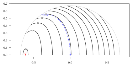
(a) $p=2$, $\mathcal{L}()$

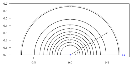
(b) $p=2$, $\psi()$

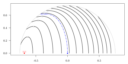
(c) $p=3$, $\mathcal{L}()$

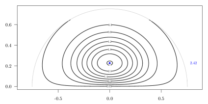
(d) $p=3$, $\psi()$

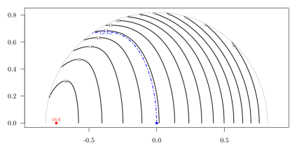
(e) $p=4$, $\mathcal{L}()$

(f) $p=4$, $\psi()$

Figure 2. Isolines of the ARL function $\mathcal{L}(\alpha,\theta)$ and the left eigenfunction $\psi(\alpha,\theta)$; polar type plot with $\alpha$ being the distance of $\bm{Z}$ to zero, and $\theta$ exhibits the angle (latitude) between $\bm{Z}$ and the new mean $\bm{\mu}_{1}$ with $\|\bm{\mu}_{1}\|=1$; $p\in\{2,3,4\}$.

(a) $p=5$, $\mathcal{L}()$

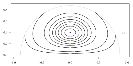
(b) $p=5$, $\psi()$

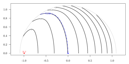
(c) $p=10$, $\mathcal{L}()$

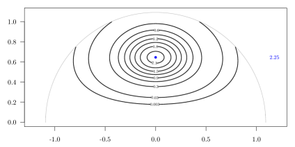
(d) $p=10$, $\psi()$

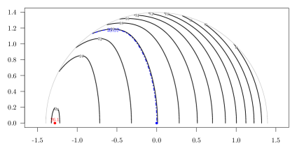
(e) $p=20$, $\mathcal{L}()$

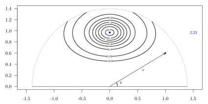
(f) $p=20$, $\psi()$

Figure 3. Isolines of the ARL function $\mathcal{L}(\alpha,\theta)$ and the left eigenfunction $\psi(\alpha,\theta)$; polar type plot with $\alpha$ being the distance of $\bm{Z}$ to zero, and $\theta$ exhibits the angle (latitude) between $\bm{Z}$ and the new mean $\bm{\mu}_{1}$ with $\|\bm{\mu}_{1}\|=1$; $p\in\{5,10,20\}$.

The six ARL plots look similarly. Even the single point labeling the maximum out-of-control ARL yields a nearly constant (relative to the threshold) position. The maps of $\psi()$ start with circular isolines for $p=2$ (remember the “exponential” shape of $\mathring{\psi}()$ and $d(\theta)=1/\pi$). Then the probability mass wanders along the $\theta=\pi/2$ line towards the border. Overlaying the two maps we conclude that approaching the worst-case becomes less likely for increasing dimension. In consequence, typical detection delays will be close to the steady-state ARL, $\mathcal{D}$, which itself differs not much from the zero-state ARL.

Now, we want to compare results of all three ARL types for various values of $\delta=\bm{\mu}^{\prime}\bm{\mu}$ (and not only one particular change $\bm{\mu}_{1}$). In order to do so, we take from Prabhu and Runger, (1997) several configurations for $\lambda=0.1$ and $E_{\infty}(N)=200$. Recall that these authors utilized a bivariate Markov chain to approximate the stationary distribution and the ARL function $\mathcal{L}()$. The corresponding matrix exhibits dimensions from 1 500 ($m=30$) up to 6 000 ($m=60$).

Table 2. ARL for $\lambda=0.1$ and $p\in\{2,3,4,10\}$; PR1997 refers to Prabhu and Runger, (1997), K2017 to Knoth, (2017), and MC to Monte Carlo ($10^{9}$ replications);  — new approach.

	zero-state			steady-state
$\sqrt{\delta}$	PR1997	K2017	MC	PR1997	$\mathcal{D}$,	$\mathcal{D}$, MC	$\mathcal{D}_{\star}$,	$\mathcal{D}_{\star}$, MC
$p=2$, $h_{4}=8.64$
0	199.98	200.54	200.54	200.03	193.09	193.09	193.29	193.29
0.5	28.07	28.02	28.02	26.87	26.79	26.79	26.82	26.82
1	10.15	10.13	10.13	9.71	9.68	9.68	9.69	9.69
1.5	6.11	6.09	6.09	5.85	5.83	5.83	5.84	5.84
2	4.42	4.41	4.41	4.23	4.22	4.22	4.23	4.23
3	2.93	2.92	2.92	2.81	2.81	2.80	2.81	2.81
$p=3$, $h_{4}=10.784$
0	–	200.03	200.03	–	191.86	191.86	192.09	192.09
0.5	–	31.85	31.85	–	30.22	30.22	30.26	30.26
1	–	11.24	11.24	–	10.60	10.60	10.62	10.62
1.5	–	6.71	6.71	–	6.31	6.31	6.32	6.32
2	–	4.83	4.83	–	4.54	4.54	4.54	4.54
3	–	3.19	3.19	–	2.99	2.99	3.00	3.00
$p=4$, $h_{4}=12.73$
0	200.12	200.50	200.50	200.05	191.82	191.82	192.07	192.07
0.5	35.11	35.07	35.07	33.12	33.11	33.11	33.16	33.16
1	12.17	12.15	12.15	11.38	11.36	11.36	11.38	11.38
1.5	7.22	7.20	7.20	6.70	6.69	6.69	6.70	6.70
2	5.19	5.18	5.18	4.80	4.79	4.79	4.80	4.80
3	3.41	3.41	3.41	3.14	3.14	3.14	3.14	3.14
$p=10$, $h_{4}=22.67$
0	199.95	200.77	200.76	200.06	190.38	190.38	190.72	190.72
0.5	48.52	48.54	48.54	44.19	45.17	45.17	45.27	45.27
1	15.98	15.93	15.93	14.32	14.47	14.47	14.51	14.51
1.5	9.23	9.21	9.21	8.23	8.21	8.21	8.24	8.24
2	6.57	6.56	6.56	5.83	5.77	5.77	5.79	5.79
3	4.28	4.28	4.28	3.79	3.70	3.70	3.71	3.71

We added the zero-state results to allow a comparison of both the potentially different accuracies between zero-state and steady-state ARL and, of course, of the levels itselves for the considered $\delta$. First, we conclude that Prabhu and Runger, (1997) really determined the cyclical steady-state ARL, $\mathcal{D}_{\star}$. Second, we recognize similar accuracy differences between the Markov chain approach of Prabhu and Runger, (1997) and the methods deploying Nyström with Gauß-Legendre quadrature for either ARL type. The Monte Carlo confirmation runs with $10^{9}$ replications confirm the validity of the latter procedures. Note that all Nyström results are based on $r=30$ nodes resulting in linear equations systems of dimension 30 and 900, respectively. Hence, the new method provides higher accuracy with smaller matrix dimensions which means less computing time. Eventually, the differences between conditional and cyclical steady-state ARL are little so that both could be applied for judging the long time behavior of MEWMA control charts.

Next, we want to illustrate the dependence of the ARL to the shift magnitude $\delta$ utilizing all three ARL types. Looking at the ARL maps we conjecture that the worst-case ARL is realized for $\theta=\pi$ ($\gamma=-1$) and some $\alpha$ close to the normalized threshold $h$. In the sequel we apply therefore golden section search to identify the final $\alpha$ yielding the maximum $\mathcal{L}(\alpha,-1)$ from (10). As in Table 2 we plot the ARL against $\sqrt{\delta}=\|\bm{\mu}\|\in(0,3.5)$.

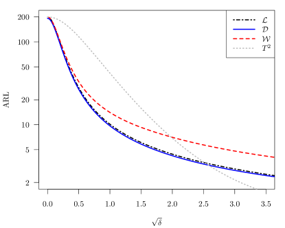
(a) $p=2$

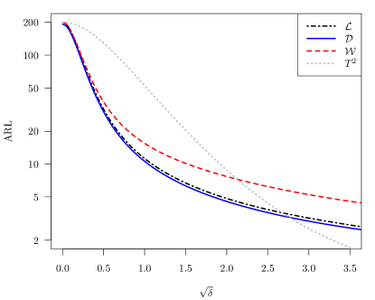
(b) $p=3$

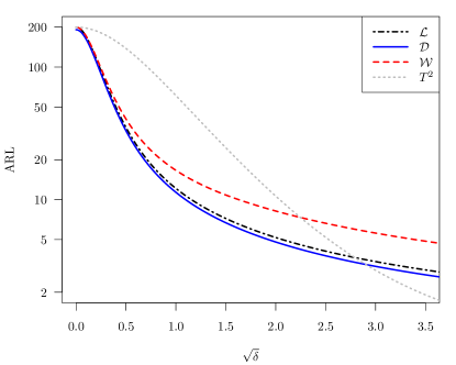
(c) $p=4$

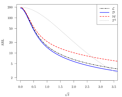
(d) $p=10$

Figure 4. Diverse ARL (zero-state $\mathcal{L}$, steady-state $\mathcal{D}$, worst-case $\mathcal{W}$) of MEWMA with $\lambda=0.1$, and of Hotelling’s ($T^{2}$) Shewhart-type chart vs. $\sqrt{\delta}=\sqrt{\|\bm{\mu}\|}$; $E_{\infty}(N)=200$.

In Figure 4, we provide all three ARL types of MEWMA charts with $\lambda=0.1$ and in-control ARL 200. In addition, we plot the respective single curves of the Shewhart-type Hotelling chart which corresponds to $\lambda=1$ and deploys only the most recent observation to decide whether signaling or not.

MEWMA clearly dominates the classic Hotelling chart for change magnitudes $\sqrt{\delta}<2$. In case of dimension $p=10$ it remains valid even for $\sqrt{\delta}<2.5$. Increasing the dimension beyond 10, we would see the MEWMA dominance over the whole interval $(0,3.5)$ which is not really surprising because an increase in $p$ while holding $\delta$ means that the shift in relation to the vector length gets smaller. Then control charts with memory such as MEWMA gain more and more in the competition with Shewhart charts. Taking into account that the worst case is not very likely, we could claim that MEWMA performs better for $\sqrt{\delta}<2.5$ and $\sqrt{\delta}<3$, respectively.

Comparing the zero-state and the steady-state ARL, we observe their divergence for increasing dimension $p$. This is essentially driven by the subtle behavior of the steady-state density of the MEWMA statistic, see Figure 3, which counterbalances the increased difficulty of detecting a change of magnitude $\delta$ for increased $p$ by moving the probability mass to favorable regions. The distance between the zero-state and the worst-case ARL remains stable. Note that the ARL values are plotted on a log-scale, hence we observe constant ratios between $\mathcal{W}$ and $\mathcal{L}$.

In order to comprehend the influence of $\lambda$ to the ARL performance, we study the relationship between $\lambda$ and the respective ARL type for one specific change, $\delta=1$. Ideally, we could derive some design rules as in Prabhu and Runger, (1997), Table 2, where the authors propose for $\delta=1$ and $E_{\infty}(N)=500$ the values 0.105 and 0.085 for dimensions $p=4$ and $10$, respectively, aiming at minimal $\mathcal{L}$. The slightly more precise numbers deploying the Gauß-Legendre Nyström methods would be 0.104 and 0.086, respectively. In Figure 5 we illustrate the hunt for optimal $\lambda$ while minimizing all three ARL types separately. Here we assume again $E_{\infty}(N)=200$ pointing out that the optimal $\lambda$ would be smaller for larger $E_{\infty}(N)$ as already indicated in Prabhu and Runger, (1997).

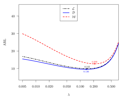
(a) $p=2$

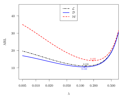
(b) $p=3$

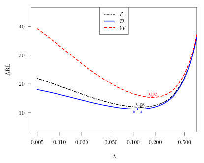
(c) $p=4$

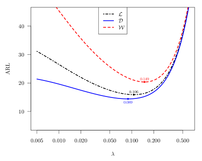
(d) $p=10$

Figure 5. Striving for optimal $\lambda$ in terms of zero-state $\mathcal{L}$, steady-state $\mathcal{D}$, and worst-case $\mathcal{W}$ of MEWMA while detecting change from $\bm{0}$ to $\bm{\mu}_{1}$ with $\|\bm{\mu}_{1}\|=1$; $E_{\infty}(N)=200$.

First, we recognize that the smallest $\lambda$ is obtained while minimizing the steady-state ARL $\mathcal{D}$ closely followed by the zero-state ARL $\mathcal{L}$ one. The optimal $\lambda$ for the worst-case ARL $\mathcal{W}$ is substantially larger. We want to emphasize that all MEWMA curves are well below the corresponding ARL values of the Hotelling chart which are 41.9, 52.4, 61.0, and 92.5, respectively. Even the (optimal) worst-case results are substantially smaller (12.7, 14.2, 15.4, and 20.4, respectively). Second, we observe like Prabhu and Runger, (1997) that for increasing dimension $p$ the optimal $\lambda$ decreases for all three ARL types. Interestingly, for large $p$ the profiles of $\mathcal{D}$ differ from the other ones considerably. It is even more pronounced, if $p$ becomes really large. Going beyond $p=30$, the profile is not convex for small $\lambda$ anymore. That is, the related values of $\mathcal{D}$ decrease with respect to $\lambda$ so that the optimal $\lambda$ might be hidden behind $\lambda<0.005$. This anomaly is known for dealing with minimizing $\mathcal{L}$ for one-sided variance EWMA schemes – see, e. g., Knoth, (2006). However, this time it is observed for the steady-state ARL $\mathcal{D}$. We remind that this peculiar behavior is caused by the patterns of the steady-state density $\psi()$ for large $p$ illustrated in Figure 3. In summary, choices of $\lambda$ within $(0.1,0.2)$ which are popular in the univariate setup turn out to be also appropriate recommendations for MEWMA. If $\delta$ is smaller or larger than 1, then, of course, $\lambda$ has to be decreased or increased accordingly.

5. Conclusions

In summary, the toolbox for calculating MEWMA ARL values is now complete. One could use either the neat Markov chain approximation introduced in Runger and Prabhu, (1996) and expanded in Prabhu and Runger, (1997) for the dealing with the steady-state ARL $\mathcal{D}$, or the highly specialized numerical algorithms for diverse integral equations proposed in Rigdon, 1995a ; Rigdon, 1995b , modified in Knoth, (2017), and extended for $\mathcal{D}$ (and $\mathcal{D}_{\star}$) in this work. For the second option, all needed routines are implemented in the R-package spc. We demonstrated the differences between the three considered ARL types — the classic zero-state ARL $\mathcal{L}$, the conditional steady-state ARL $\mathcal{D}$, and the worst-case ARL $\mathcal{W}$ — and their different impact to the choice of the chart constant $\lambda$. For large dimension $p$, eventually, we illustrated the odd behavior of the MEWMA statistic reaching the steady-state. Note that the decomposition idea in Lemma 1 could be utilized also to calculate the expected detection delays $D_{\tau}:=E_{\tau}\big{(}N-\tau+1\mid N\geq\tau\big{)}$ for $\tau=(1,)2,3,\ldots$ The resulting sequence $\{D_{\tau}\}$ allows to evaluate the convergence patterns of $D_{\tau}\to\mathcal{D}$ and consequently to judge the validity of the measure $\mathcal{D}$.

Appendix A Linear equation systems

First we plug in the Gauß-Legendre weights $w_{i}$ and nodes $z_{i}$ into (5) after replacing $\alpha$ by $\alpha^{2}$, $u$ by $u^{2}$, and $\mathrm{d}u$ by $2u\,\mathrm{d}u$ so that we obtain

$$\bm{\mathring{\ell}} =(\mathring{\ell}_{1},\ldots,\mathring{\ell}_{r})^{\prime}\;,\;\;\mathring{\ell}_{i}=\mathcal{\mathring{L}}(z_{i}^{2})\;,\;\;\mathbb{Q}_{\mathcal{L}}=(q_{ij}^{\mathcal{L}})_{i,j=1,\ldots,r}\;,$$

$$\qquad q_{ij}^{\mathcal{L}}=w_{j}\frac{1}{\lambda^{2}}f_{\chi^{2}}\left(\frac{z_{j}^{2}}{\lambda^{2}}\,\Big{|}\,p,\eta z_{i}^{2}\right)2z_{j}\,,$$

$$\bm{\mathring{\ell}} =(\mathbb{I}-\mathbb{Q}_{\mathcal{L}})^{-1}\bm{1}\,,$$

and similarly for the left eigenfunctions

$$\bm{\mathring{\psi}} =(\mathring{\psi}_{1},\ldots,\mathring{\psi}_{r})^{\prime}\;,\;\;\mathring{\psi}_{i}=\mathring{\psi}(z_{i}^{2})\;,\;\;\mathbb{Q}_{\psi}=(q_{ij}^{\psi})_{i,j=1,\ldots,r}\;$$

$$\qquad q_{ij}^{\psi}=w_{j}\frac{1}{\lambda^{2}}f_{\chi^{2}}\left(\frac{z_{i}^{2}}{\lambda^{2}}\,\Big{|}\,p,\eta z_{j}^{2}\right)2z_{j}\,,$$

$$\varrho\bm{\mathring{\psi}} =\mathbb{Q}_{\psi}\bm{\mathring{\psi}}\qquad\text{... power method or standard eigenvalue procedure.}$$

$$\bm{\mathring{\psi}}_{\star} =(\mathring{\psi}_{1}^{\star},\ldots,\mathring{\psi}_{r}^{\star})^{\prime}\;,\;\;\mathring{\psi}_{i}^{\star}=\mathring{\psi}_{\star}(z_{i}^{2})\;,\;\;\bm{\mathring{\psi}}_{\star}=(\mathbb{I}-\mathbb{Q}_{\psi})^{-1}\bm{f}\qquad\text{... see \eqref{eq:psi0ble}.}$$

Note that $\bm{\mathring{\psi}}$ and $\bm{\mathring{\psi}}_{\star}$ rely on the same matrix $\mathbb{Q}_{\psi}$. Applying the Markov chain approximation as in Prabhu and Runger, (1997), one would observe $\mathbb{Q}_{\psi}=\mathbb{Q}_{\mathcal{L}}^{\prime}$ for the corresponding Markov chain transition matrix.

Appendix B Transformation of ARL integral equation

Change integration order in

$$\mathcal{L}(\alpha,\beta) =1+\int_{-\sqrt{\delta h}}^{\sqrt{\delta h}}\int_{v^{2}/\delta}^{h}\mathcal{L}(u,v)K(u,v;\alpha,\beta)\,\mathrm{d}u\,\mathrm{d}v$$

$$=1+\int_{0}^{h}\int_{-\sqrt{\delta u}}^{\sqrt{\delta u}}\mathcal{L}(u,v)K(u,v;\alpha,\beta)\,\mathrm{d}v\,\mathrm{d}u\,,$$

$$K(u,v;\alpha,\beta) =\frac{1}{\sqrt{2\pi\delta\lambda^{2}}}e^{-\frac{[v-\lambda\delta-(1-\lambda)\beta]^{2}}{2\delta\lambda^{2}}}\frac{1}{\lambda^{2}}f_{\chi^{2}}\left(\!\frac{u-v^{2}/\delta}{\lambda^{2}}\,\Big{|}\,p-1,\eta(\alpha-\beta^{2}/\delta)\!\right)\,.$$

Change second argument

$$\beta =\sqrt{\alpha\delta}\,\gamma\;,\;\;v=\sqrt{u\delta}\,w\;,\;\;\mathrm{d}v=\sqrt{u\delta}\,\mathrm{d}w\;,\;\;w=v/\sqrt{\delta u}\,,$$

so that

$$\mathcal{L}(\alpha,\gamma) =1+\int_{0}^{h}\int_{-1}^{1}\mathcal{L}(u,w)K^{\dagger}(u,w;\alpha,\gamma)\,\mathrm{d}w\,\mathrm{d}u\,,$$

$$K^{\dagger}(u,w;\alpha,\gamma) =\frac{\sqrt{u}}{\sqrt{2\pi\lambda^{2}}}e^{-\frac{[\sqrt{u}w-\lambda\sqrt{\delta}-(1-\lambda)\sqrt{\alpha}\gamma]^{2}}{2\lambda^{2}}}$$

$$\qquad\times\frac{1}{\lambda^{2}}f_{\chi^{2}}\left(\frac{u(1-w^{2})}{\lambda^{2}}\,\Big{|}\,p-1,\eta\alpha(1-\gamma^{2})\right)\,.$$

Appendix C Numerics of ARL integral equation

Let $(z^{(0)}_{i},w^{(0)}_{i})$ and $(z^{(1)}_{j},w^{(1)}_{j})$ be the quadrature nodes and weights on $[0,h]$ and $[-1,1]$, respectively. Then we solve the following linear equation system(s).

$$\mathcal{L}_{ij} =\mathcal{L}(z^{(0)}_{i},z^{(1)}_{j})$$

$$=1+\frac{1}{\lambda^{3}\sqrt{2\pi}}\sum_{k=1}^{N}w^{(0)}_{k}\sqrt{z^{(0)}_{k}}\sum_{l=1}^{N}w^{(1)}_{l}e^{-\frac{\left[\sqrt{z^{(0)}_{k}}z^{(1)}_{l}-\lambda\sqrt{\delta}-(1-\lambda)\sqrt{z^{(0)}_{i}}z^{(1)}_{j}\right]^{2}}{2\lambda^{2}}}\ldots$$

$$\qquad\times f_{\chi^{2}}\left(\frac{z^{(0)}_{k}\big{(}1-(z^{(1)}_{l})^{2}\big{)}}{\lambda^{2}}\,\Big{|}\,p-1,\eta z^{(0)}_{i}\big{(}1-(z^{(1)}_{j})^{2}\big{)}\right)\,.$$

w/ $$u u^{2} w \sin(w)$$ to and to in (10):

$$=1+\frac{1}{\lambda^{3}\sqrt{2\pi}}\sum_{k=1}^{N}w^{(0)}_{k}2(z^{(0)}_{k})^{2}\sum_{l=1}^{N}w^{(1)}_{l}\cos(z^{(1)}_{l})\,e^{-\frac{\left[z^{(0)}_{k}\sin(z^{(1)}_{l})-\lambda\sqrt{\delta}-(1-\lambda)z^{(0)}_{i}\sin(z^{(1)}_{j})\right]^{2}}{2\lambda^{2}}}\ldots$$

$$\qquad\times f_{\chi^{2}}\left(\frac{(z^{(0)}_{k})^{2}\big{(}\cos(z^{(1)}_{l})\big{)}^{2}}{\lambda^{2}}\,\Big{|}\,p-1,\eta(z^{(0)}_{i})^{2}\big{(}\cos(z^{(1)}_{j})\big{)}^{2}\right)\,.$$

Appendix D Angle distribution

From standard math literature we obtain for the surface area on the unit sphere $S^{p-1}$

$$A_{p-1}=\frac{2\pi^{\frac{p}{2}}}{\Gamma\left(\frac{p}{2}\right)}\;,\;\;p=1,2,\ldots$$

This surface is assembled by a continuous set of circles of latitude which are spheres of one dimension less whose radius depends on the latitude. Their area depending on latitude $\theta\in[0,\pi]$ with related radius $\sin(\theta)$ follows

$$\tilde{A}_{p-2}(\theta)=\frac{2\pi^{\frac{p-1}{2}}}{\Gamma\left(\frac{p-1}{2}\right)}\sin(\theta)^{p-2}\;,\;\;p=2,3,\ldots$$

Now we derive the density of $\theta$ using the proportion of $\tilde{A}_{p-2}(\theta)$ relative to $A_{p-1}$:

$$d(\theta)=\frac{\tilde{A}_{p-2}(\theta)}{A_{p-1}}=\frac{\Gamma\left(\frac{p}{2}\right)}{\Gamma\left(\frac{p-1}{2}\right)\sqrt{\pi}}\sin(\theta)^{p-2}\,.$$

Applying the transformation $\gamma=-\cos(\theta)$ we get

$$\theta =\text{acos}(-\gamma)\;,\;\;\frac{\mathrm{d}}{\mathrm{d}\theta}\gamma(\theta)=\sin(\theta)=\sin\big{(}\text{acos}(-\gamma)\big{)}=\sqrt{1-\gamma^{2}}\,.$$

$$d(\gamma) =\frac{\Gamma(\frac{p}{2})}{\Gamma(\frac{p-1}{2})}(1-\gamma^{2})^{\frac{p-3}{2}}/\sqrt{\pi}\;,\;\;\gamma\in(-1,1]\,.$$

Appendix E Proof supporting Lemma 1

First, we make use of the following presentation of the non-central $\chi^{2}$ density, which was mentioned already in Venables, (1973), equation (2.10):

$$f_{\chi^{2}}(x\mid p,\nu)=e^{-(x+\nu)/2}\frac{x^{p/2-1}}{2^{p/2}\Gamma(p/2)}\,{{}_{0}}F_{1}(;p/2;\nu x/4)\,.$$

Thereby, ${{}_{0}}F_{1}(;b;z)$ is called confluent hypergeometric limit function and is closely related to Bessel functions. To get an idea about ${{}_{0}}F_{1}()$, we give one presentation:

$${{}_{0}}F_{1}(;b;z)=\sum_{n=0}^{\infty}\frac{z^{n}}{(b)_{n}\,n!}\;\text{ with }\;(b)_{n}=b(b+1)\cdots(b+n-1)\;\;\text{\small(Pochhammer symbol)}\,.$$

A more rigor discussion with proofs is given in Muirhead, (1982), Theorem 1.3.4. Taking these subtleties aside, we start with

$$\lambda^{2}(1-\gamma^{2})^{\frac{p-3}{2}}K^{\dagger}(u,w;\alpha,\gamma)$$

$$=(1-\gamma^{2})^{\frac{p-3}{2}}\frac{\sqrt{u}}{\sqrt{2\pi\lambda^{2}}}e^{-\frac{[\sqrt{u}w-(1-\lambda)\sqrt{\alpha}\gamma]^{2}}{2\lambda^{2}}}f_{\chi^{2}}\left(\frac{u(1-w^{2})}{\lambda^{2}}\,\Big{|}\,p-1,\eta\alpha(1-\gamma^{2})\right)$$

$$=(1-\gamma^{2})^{\frac{p-3}{2}}\frac{\sqrt{u}}{\sqrt{2\pi\lambda^{2}}}e^{-\frac{uw^{2}-2\sqrt{u}w(1-\lambda)\sqrt{\alpha}\gamma+(1-\lambda)^{2}\alpha\gamma^{2}}{2\lambda^{2}}}$$

$$\qquad\times e^{-\frac{u(1-w^{2})+(1-\lambda)^{2}\alpha(1-\gamma^{2})}{2\lambda^{2}}}\frac{\left(\frac{u(1-w^{2})}{\lambda^{2}}\right)^{p/2-1}}{2^{p/2}\Gamma(p/2)}$$

$$\qquad\qquad\times{{}_{0}F_{1}}\left(;\frac{p-1}{2};\frac{u(1-w^{2})(1-\lambda)^{2}\alpha(1-\gamma^{2})}{4\lambda^{4}}\right)\,.$$

Rearrange variables:

$$=(1-w^{2})^{\frac{p-3}{2}}\frac{\sqrt{u}}{\sqrt{2\pi\lambda^{2}}}e^{-\frac{u\gamma^{2}-2\sqrt{u}\gamma(1-\lambda)\sqrt{\alpha}w+(1-\lambda)^{2}\alpha w^{2}}{2\lambda^{2}}}$$

$$\qquad\times e^{-\frac{u(1-\gamma^{2})+(1-\lambda)^{2}\alpha(1-w^{2})}{2\lambda^{2}}}\frac{\left(\frac{u(1-\gamma^{2})}{\lambda^{2}}\right)^{p/2-1}}{2^{p/2}\Gamma(p/2)}$$

$$\qquad\qquad\times{{}_{0}F_{1}}\left(;\frac{p-1}{2};\frac{u(1-\gamma^{2})(1-\lambda)^{2}\alpha(1-w^{2})}{4\lambda^{4}}\right)$$

$$=(1-w^{2})^{\frac{p-3}{2}}\frac{\sqrt{u}}{\sqrt{2\pi\lambda^{2}}}e^{-\frac{[\sqrt{u}\gamma-(1-\lambda)\sqrt{\alpha}w]^{2}}{2\lambda^{2}}}f_{\chi^{2}}\left(\frac{u(1-\gamma^{2})}{\lambda^{2}}\,\Big{|}\,p-1,\eta\alpha(1-w^{2})\right)\,.$$

Now we are ready to perform the integration:

$$\left((1-w^{2})^{\frac{p-3}{2}}\right)^{-1}\lambda^{2}\int_{-1}^{1}(1-\gamma^{2})^{\frac{p-3}{2}}K^{\dagger}(u,w;\alpha,\gamma)\,\mathrm{d}\gamma$$

$$=\int_{-1}^{1}\frac{\sqrt{u}}{\sqrt{2\pi\lambda^{2}}}e^{-\frac{[\sqrt{u}\gamma-(1-\lambda)\sqrt{\alpha}w]^{2}}{2\lambda^{2}}}f_{\chi^{2}}\left(\frac{u(1-\gamma^{2})}{\lambda^{2}}\,\Big{|}\,p-1,\eta\alpha(1-w^{2})\right)\,\mathrm{d}\gamma$$

$$=\int_{-\sqrt{u}}^{\sqrt{u}}\frac{1}{\sqrt{2\pi\lambda^{2}}}e^{-\frac{[\tilde{\gamma}-(1-\lambda)\sqrt{\alpha}w]^{2}}{2\lambda^{2}}}f_{\chi^{2}}\left(\frac{u-\tilde{\gamma}^{2}}{\lambda^{2}}\,\Big{|}\,p-1,\eta\alpha(1-w^{2})\right)\,\mathrm{d}\tilde{\gamma}$$

$$=f_{\chi^{2}}\left(\frac{u}{\lambda^{2}}\,\Big{|}\,p,\eta\alpha\right)\,.$$

The last integral follows from summing two $\chi^{2}$ variates, $G\sim\mathcal{N}\big{(}(1-\lambda)\sqrt{\alpha}w,\lambda^{2}\big{)}$ and $V/\lambda^{2}\sim\chi^{2}_{p-1,\eta\alpha(1-w^{2})}$. Then for the sum we observe $(G^{2}+V)/\lambda^{2}\sim\chi^{2}_{p,\eta\alpha}$. Finally, moving the terms before the integral to the right-hand side yields

$$\int_{-1}^{1}(1-\gamma^{2})^{\frac{p-3}{2}}K^{\dagger}(u,w;\alpha,\gamma)\,\mathrm{d}\gamma =(1-w^{2})^{\frac{p-3}{2}}\frac{1}{\lambda^{2}}f_{\chi^{2}}\left(\frac{u}{\lambda^{2}}\,\Big{|}\,p,\eta\alpha\right)\,.$$

References

- Anderson et al., (1999) Anderson, E., Bai, Z., Bischof, C., Blackford, S., Demmel, J., Dongarra, J., Croz, J. D., Greenbaum, A., Hammarling, S., McKenney, A., and Sorensen, D. (1999). LAPACK Users’ Guide. Society for Industrial and Applied Mathematics, Philadelphia, PA, third edition.
- Crosier, (1986) Crosier, R. B. (1986). A new two-sided cumulative quality control scheme. Technometrics, 28(3):187–194.
- Darroch and Seneta, (1965) Darroch, J. N. and Seneta, E. (1965). On quasi-stationary distributions in absorbing discrete-time finite Markov chains. Journal of Applied Probability, 2(1):88–100.
- Gold, (1989) Gold, M. S. (1989). The geometric approximation to the CUSUM run length distribution. Biometrika, 76(4):725–733.
- Harrou et al., (2018) Harrou, F., Sun, Y., Taghezouit, B., Saidi, A., and Hamlati, M.-E. (2018). Reliable fault detection and diagnosis of photovoltaic systems based on statistical monitoring approaches. Renewable Energy, 116:22–37.
- Hotelling, (1947) Hotelling, H. (1947). Multivariate quality control illustrated by the air testing of sample bombsights. In Techniques of Statistical Analysis, pages 111–184. New York: McGraw Hill.
- Knoth, (2006) Knoth, S. (2006). The art of evaluating monitoring schemes – how to measure the performance of control charts? In Lenz, H.-J. and Wilrich, P.-T., editors, Frontiers in Statistical Quality Control 8, pages 74–99. Physica Verlag, Heidelberg, Germany.
- Knoth, (2016) Knoth, S. (2016). The case against the use of synthetic control charts. Journal of Quality Technology, 48(2):178–195.
- Knoth, (2017) Knoth, S. (2017). ARL numerics for MEWMA charts. Journal of Quality Technology, 49(1):78–89.
- Lawson et al., (1979) Lawson, C. L., Hanson, R. J., Kincaid, D. R., and Krogh, F. T. (1979). Basic linear algebra subprograms for FORTRAN usage. ACM Transactions on Mathematical Software, 5(3):308–323.
- Lee and Khoo, (2014) Lee, M. H. and Khoo, M. B. C. (2014). Design of a multivariate exponentially weighted moving average control chart with variable sampling intervals. Computational Statistics, 29(1-2):189–214.
- Lowry et al., (1992) Lowry, C. A., Woodall, W. H., Champ, C. W., and Rigdon, S. E. (1992). A multivariate exponentially weighted moving average control chart. Technometrics, 34(1):46–53.
- Moustakides et al., (2009) Moustakides, G. V., Polunchenko, A. S., and Tartakovsky, A. G. (2009). Numerical comparison of CUSUM and Shiryaev–Roberts procedures for detecting changes in distributions. Communications in Statistics – Theory and Methods, 38(16-17):3225–3239.
- Muirhead, (1982) Muirhead, R. J. (1982). Aspects of multivariate statistical theory. John Wiley & Sons.
- Nyström, (1930) Nyström, E. J. (1930). Über die praktische Auflösung von Integralgleichungen mit Anwendungen auf Randwertaufgaben. Acta Mathematica, 54(1):185–204.
- Page, (1954) Page, E. S. (1954). Control charts for the mean of a normal population. Journal of the Royal Statistical Society: Series B (Statistical Methodology), 16(1):131–135.
- Pollak and Tartakovsky, (2009) Pollak, M. and Tartakovsky, A. G. (2009). Optimality properties of the Shiryaev-Roberts procedure. Statistica Sinica, 19(4):1729–1739.
- Prabhu and Runger, (1997) Prabhu, S. S. and Runger, G. C. (1997). Designing a multivariate EWMA control chart. Journal of Quality Technology, 29(1):8–15.
- Reynolds Jr. and Stoumbos, (2008) Reynolds Jr., M. R. and Stoumbos, Z. G. (2008). Combinations of multivariate Shewhart and MEWMA control charts for monitoring the mean vector and covariance matrix. Journal of Quality Technology, 40(4):381–393.
- (20) Rigdon, S. E. (1995a). An integral equation for the in-control average run length of a multivariate exponentially weighted moving average control chart. J. Stat. Comput. Simulation, 52(4):351–365.
- (21) Rigdon, S. E. (1995b). A double-integral equation for the average run length of a multivariate exponentially weighted moving average control chart. Stat. Probab. Lett., 24(4):365–373.
- Roberts, (1966) Roberts, S. W. (1966). A comparison of some control chart procedures. Technometrics, 8(3):411–430.
- Runger and Prabhu, (1996) Runger, G. C. and Prabhu, S. S. (1996). A Markov chain model for the multivariate exponentially weighted moving averages control chart. J. Amer. Statist. Assoc., 91(436):1701–1706.
- Taylor, (1968) Taylor, H. M. (1968). The economic design of cumulative sum control charts. Technometrics, 10(3):479–488.
- Venables, (1973) Venables, W. N. (1973). Inference problems based on non-central distributions. PhD thesis, Department of Statistics, University of Adelaide.
- von Mises and Pollaczek-Geiringer, (1929) von Mises, R. and Pollaczek-Geiringer, H. (1929). Praktische Verfahren der Gleichungsauflösung. Zeitschrift für angewandte Mathematik und Mechanik, 9(1):58–77.
- Yang et al., (2018) Yang, H.-H., Huang, M.-L., Lai, C.-M., and Jin, J.-R. (2018). An approach combining data mining and control charts-based model for fault detection in wind turbines. Renewable Energy, 115:808–816.
- Yashchin, (1985) Yashchin, E. (1985). On the analysis and design of CUSUM-Shewhart control schemes. IBM Journal of Research and Development, 29(4):377–391.
- Zou and Tsung, (2011) Zou, C. and Tsung, F. (2011). A multivariate sign EWMA control chart. Technometrics, 53(1):84–97.