Test of semi-local duality in a large $N_{C}$ framework

Abstract

In this paper we test the semi-local duality based on the method of Ref. Dai:2017uao for calculating final-state interactions at varying number of colors ($N_{C}$). We compute the amplitudes by dispersion relations that respect analyticity and coupled channel unitarity, as well as accurately describing experiment. The $N_{C}$ dependence of the $\pi\pi\to\pi\pi$ scattering amplitudes is obtained by comparing these amplitudes to the one of chiral perturbation theory. The semi-local duality is investigated by varying $N_{C}$. Our results show that the semi-local duality is not violated when $N_{C}$ is large. At large $N_{C}$, the contributions of the $f_{2}(1270)$, the $f_{0}(980)$ and the $f_{0}(1370)$ cancel that of the $\rho(770)$ in the finite energy sum rules, while the $f_{0}(500)$ has almost no effect. This gives further credit to the method developed in Ref. Dai:2017uao for investigating the $N_{C}$ dependence of hadron-hadron scattering with final-state interactions. This study is also helpful to understand the structure of the scalar mesons.

I Introduction

The $1/N_{C}$ expansion 'tHooft:1973jz ; 'tHooft:1974hx provides an effective diagnostics to differentiate the ordinary from the non-ordinary quark-antiquark structure of the mysterious scalars, see e.g. Pelaez04 ; Pelaez06 ; MRP11 ; Sun ; DLY11 . In the physical world, i.e. at $N_{C}=3$, there should be local duality Veneziano:1968yb ; Dolen:1967zz ; Dolen:1967jr ; Schmid:1968zza ; Schmid:1968zz ; Shiga:1971by . This means that Regge exchange in the crossed channel is dual to the contribution of resonances in the direct channel. One thus only needs to add either the Regge term or the direct channel resonances in a given calculation. An explicit model shows that there is no interference between these two contributions Veneziano:1968yb . Indeed, in the high-energy region the overlap of the resonances is much stronger, leading to a smooth amplitude. Such a smooth amplitude is similar to the one generated by Regge poles in the $t$-channel. The cross section is therefore more readily described by the Regge exchanges in the crossed channel rather than by lots of resonances in the direct ($s-$)channel. However, in the real world, things are more complicated as the widths of the resonances are finite and only semi-local duality is fulfilled MRP11 . Through finite-energy sum rules (FESR) the equivalence between the resonances in the direct $s$-channel and the Regge poles in the crossed $t$-channel holds on the average Schmid:1968zz ; Schmid:1968zza .

In the pioneering work of MRP11 , the semi-local duality is tested in the large $N_{C}$ case and it is shown to be useful for investigating the structure of the light scalar mesons. The scattering amplitudes are obtained by unitarized chiral perturbation theory (U$\chi$PT) and the $N_{C}$ dependence of the pertinent low-energy constants is taken over to the amplitudes. The FESR are tested by tuning $N_{C}$ up to 30 or 100. They found that the $f_{0}(500)$ (often also called the $\sigma$) should contain a sub-dominant $\bar{q}q$ component and this ensures the semi-local duality to be fulfilled up to $N_{C}=15-30$. This was later used to constrain the meson-meson scattering amplitudes calculated within $U(3)$ unitary $\chi$PT Guo:2012yt . The semi-local duality could be fulfilled very well up to $N_{C}=30$. The relation between local duality and exotic states is also discussed in Ref. Zheng:2004xw .

On the other hand, final-state interactions (FSI) play an important role in hadron phenomenology, especially when the energy is not very far away from the threshold of a pair or triplet of hadrons. For different models to describe the FSI, see e.g. AMP-FSI ; Meissner:1990kz ; Guo2011 ; Dai:2012pb ; Kang:2013uia ; Kang:2013jaa ; Garcia-Recio:2013uva ; Chen2015 ; Wilson2016 ; Colangelo:2016jmc ; Hanhart:2016pcd ; Dai:2017ont ; Cheng:2017pcq . In our earlier paper, a new method to study the large $N_{C}$ behavior of the FSI was proposed Dai:2017uao . The $N_{C}$ dependence is generated based on the fact that the tangent of the phase is proportional to $1/N_{C}$, that is, $\tan\varphi\sim\mathcal{O}(1/N_{C})$, where ${\rm Re}T\sim\mathcal{O}(1/N_{C})$ and ${\rm Im}T\sim\mathcal{O}(1/N_{C}^{2})$ are naturally given by chiral perturbation theory ($\chi$PT). The trajectories of the widths of the $\rho$ and the $f_{2}$ quantitatively behave as $1/N_{C}$, which confirms the reliability of the method. Following that work, a natural extension is to check whether the semi-local duality is satisfied using this method.

This paper is organized as follows: In Sect. II we use a dispersive method to obtain the $I=2$ $\pi\pi$ scattering partial waves up to $s\sim 4$ GeV², that were not considered in Dai:2017uao . The amplitudes are constructed analytically and respect the coupled channel unitarity and give a good description of the experimental data. In Sect. III we introduce the $N_{C}$-dependence into the dispersive amplitudes following Ref. Dai:2017uao . The semi-local duality is tested by tuning $N_{C}$ up to 180. We find that it works well when $N_{C}$ is large. The contributions of each resonance that appears in the amplitudes are also studied. Finally we give a brief summary in Sec. IV.

II Scattering amplitudes and $N_{C}$ dependence

In Ref.  Dai:2017uao , the $\pi\pi$ scattering amplitudes with $IJ=00,11,02$ (with $I/J$ the total isospin/angular momentum) have already been given. Here, we focus on the isospin-2 waves with $IJ=20,22$ to complete the analysis. All these waves are certainly needed for testing the semi-local duality. We use (for more details on the method, see Dai:2017uao ),

$$T^{I}_{J}(s)=P^{I}_{J}(s)\Omega^{I}_{J}(s)\,,$$ (1)

with $\Omega^{I}_{J}(s)$ the Omnès function Omnes1958 :

$$\Omega^{I}_{J}(s)=\exp\left(\frac{s}{\pi}\int^{\infty}_{4M_{\pi}^{2}}ds^{\prime}\frac{\varphi^{I}_{J}(s^{\prime})}{s^{\prime}(s^{\prime}-s)}\right)\,.$$ (2)

Here, $\varphi^{I}_{J}(s)$ is the phase of the partial wave amplitude $T^{I}_{J}(s)$, as given in previous amplitude analysis DLY-MRP14 ; DLY2015:1 . By a fit to the experimental data OPE1973 as well as the amplitudes of the dispersive analysis KPY , the phase is obtained up to $s=4$ GeV². Above this energy region we use unitarity to constrain it, but for practical reasons the extension is limited and we truncate the integration of the Omnès function at $s=22$ GeV². The other function $P^{I}_{J}(s)$ is represented by a series of polynomials. It absorbs the contribution from the left-hand cut (l.h.c) and the distant right-hand cut (r.h.c) above 4 GeV². To include the Adler zero in the S-wave and threshold behavior in the D-wave, in terms of the scattering length and effective range, we parameterize the $P^{I}_{J}(s)$ as

$$P^{I}_{J}(s)=(s-z^{I}_{J})^{n_{J}}\sum_{k=1}^{n}{\alpha^{I}_{J}}_{k}(s-4M_{\pi}^{2})^{k-1}\,,$$ (3)

with $z^{I}_{J}$ to be either the Adler zero for the S-wave or $4M_{\pi}^{2}$ for the D-wave. Similarly, $n_{J}$ is 1 for the S-wave and 2 for the D-wave. The fitted parameters $\alpha_{i}$ are given in Tab. 1. The units of the $\alpha_{k}$ are chosen to guarantee the amplitude $T^{I}_{J}(s)$ to be dimensionless.

	${T}^{2}_{0}(s)$	${T}^{2}_{2}(s)$
$\alpha_{1}$	$-$1.2489	0.0472
$\alpha_{2}$	2.1544	$-$0.4514
$\alpha_{3}$	$-$3.2683(7)	1.1773(1)
$\alpha_{4}$	3.2207(3)	$-$1.5165(1)
$\alpha_{5}$	$-$1.8749(1)	1.0138(1)
$\alpha_{6}$	0.6212(1)	$-$0.3587(1)
$\alpha_{7}$	$-$0.1077(1)	0.0638(1)
$\alpha_{8}$	0.0076(1)	$-$0.0045(1)

Table 1: The fit parameters corresponding to Eq. (3). The uncertainties are given by MINUIT and $\alpha_{1,2}$ are fixed by the scattering lengths and slope parameters KPY ; Ke4 .

The fit amplitudes are shown in Fig. 1 for the energy region of $s\in[0,4\,\rm{GeV}^{2}]$. What we fit to are the following contributions: $\chi$PT amplitudes for $[0,4M_{\pi}^{2}]$ Gasser1984 ; Gasser1985 ; Bijnens1994 ; Pelaez02 , amplitudes of the Roy-type equation analysis at $[4M_{\pi}^{2},2\,\rm{GeV}^{2}]$ KPY , and experiment up to $4\,\rm{GeV}^{2}$ OPE1973 . We also plot the amplitudes in the region of $s\in[-4M_{\pi}^{2},0]$. Here the real part of our amplitudes is in good agreement with that of $\chi PT$ ($\mathcal{O}(p^{4})$), and the imaginary part vanishes, which is consistent with the imaginary part of the $\chi PT$ amplitudes as the latter is rather small. These indicate the high quality of the fit.

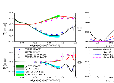
Figure 1: Left column: Fit of the isospin-2 $\pi\pi$ scattering amplitudes (solid lines). The olive and light grey bands in the low-energy region are from $\chi$PT Gasser1984 ; Gasser1985 ; Bijnens1994 ; Pelaez02 . The cyan and green bands are from CFDIV KPY . The OPE and OPE-DP data are from OPE1973 . Right column: The absolute values of the amplitudes by varying $N_{C}$ are shown. The black solid, orange dashed, blue dotted and magenta dash-dotted lines are for $N_{C}=3,6,12,120$, respectively.

As is well known, the Roy-type equation analysis embodies crossing symmetry, which is lacking in Eq. (1). Therefore, following Dai:2017tew , we fit our amplitudes to the ‘data’ on the real axis as well as the amplitudes given by the Roy-like equation KPY in the complex $s$-plane. As shown in Fig. 2, the two $T_{0}^{2}$ amplitudes are compatible with each other except for the region where $s$ is too large (either ${\rm Re}[s]>1.0$ GeV² or ${\rm Im}[s]<-0.3$ GeV²). We note that the amplitudes on the upper half of $s$-plane are readily obtainable from the ones on the lower side according to the Schwarz reflection principle. The distribution of contours is in good agreement and moreover, their gradient variations are compatible with each other, as shown by the shading of the color from blue to red. Nevertheless, above 1.0 GeV our amplitudes are a bit different from that of the dispersive analysis, while both of them are in compatible with the data, see in Fig.1. Also our amplitudes in the bottom-right direction, where either $\rm{Re}[s]$ or $\rm{Im}[s]$ is large, are becoming less consistent with differences $\leq 0.1$.

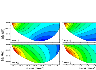
Figure 2: Comparison of our amplitudes ($IJ=20$) with the ones from the Roy-like equation analysis in the domain where the Roy equations work. On the left side there are real and imaginary parts of our amplitudes, and on the right side those are from Roy like equations KPY .

Now that these amplitudes are obtained for the physical world, that is for $N_{C}=3$, we can introduce the $N_{C}$ dependence. Apparently, the real part of the $\chi$PT amplitude is $\mathcal{O}(N_{C}^{-1})$ and the imaginary part is $\mathcal{O}(N_{C}^{-2})$ up to any order. Therefore, we generate the $N_{C}$ dependence as Dai:2017uao :

$$\varphi(s,N_{C})\;=\;\arctan\left[\frac{3}{N_{C}}\tan\varphi(s)\right]\;,$$ (4)

and

$$P^{I}_{J}(s,N_{C})\;=\;\frac{3}{N_{C}}P^{I}_{J}(s)\;.$$ (5)

It is not difficult to check that at large $N_{C}$ the phase, which would return back to the phase shift in a single channel, will jump by $\pi$ around $s=M_{R}^{2}$ where $\varphi(M_{R}^{2})=90^{\circ}$. This is consistent with the large $N_{C}$ property of a simple Breit-Wigner formalism or the “narrow resonance pole” on the second Rieman sheet Guo:2007ff . All the complicated higher-order $N_{C}$ dependence is ignored for simplicity. By increasing $N_{C}$, the magnitude of the $I=2$ S-wave and D-wave become smaller and smaller, as shown in Fig. 1. This is consistent with the fact that there is no resonance in the $I=2$ channel.

III Semi-local duality

We follow Ref. MRP11 to calculate the variation of the FESR by tuning $N_{C}$. It is well-known that the $t$-channel $\pi\pi$ scattering amplitudes could be written in terms of the $s$-channel ones according to the crossing relations

$$T^{I_{t}}(s,t)=\sum_{I^{\prime}_{s}=0}^{2}C_{st}^{I_{t}I^{\prime}_{s}}T^{I^{\prime}_{s}}(s,t)\,,$$

where $I$ denotes the total isospin $(I=0,1,2)$ of the $\pi\pi$-system and $C_{st}$ is the orthogonal crossing matrix

$$C_{st}=C_{ts}=\left(\begin{array}[]{c c c}\displaystyle 1/3&\displaystyle 1&\displaystyle 5/3\\ \displaystyle 1/3&\displaystyle 1/2&\displaystyle-5/6\\ \displaystyle 1/3&\displaystyle-1/2&\displaystyle 1/6\end{array}\right)\,.$$ (9)

The $s$-channel amplitude is composed of a complete set of partial waves

$$T^{I_{s}}(s,t)=\sum_{J}(2J+1)T_{J}^{I_{s}}(s)P_{J}(\cos\theta_{s})\,,$$

with $\theta_{s}$ the $s$-channel scattering angle in the center of mass frame. Of course, $I_{s}+J$ should be even as required by Bose symmetry and isospin conservation. Higher partial waves are less known and we restrict our amplitudes up to the D-waves.

We introduce the function

$$F^{I_{t}}_{n}(\nu,t)={\rm Im}T^{I_{t}}(\nu,t)\nu^{-n}\,,$$ (10)

with $\nu=(s-u)/2$. We note that when $t=4M_{\pi}^{2}$, $\nu=s=-u$. Semi-local duality implies that the contribution of Regge exchange and of resonances are dual with each other on the average,

$$\int_{\nu_{1}}^{\nu_{2}}d\nu F^{I_{t}}_{n}(\nu,t)_{\rm resonances}\simeq\int_{\nu_{1}}^{\nu_{2}}d\nu F^{I_{t}}_{n}(\nu,t)_{\rm Regge}\,.$$ (11)

To test duality in the large $N_{C}$ limit, we first estimate it at $N_{C}=3$. It is helpful to introduce the ratio MRP11

$$R^{I}_{n}(t)=\frac{\int_{\nu_{1}}^{\nu_{2}}d\nu F^{I_{t}}_{n}(\nu,t)}{\int_{\nu_{1}}^{\nu_{3}}d\nu F^{I_{t}}_{n}(\nu,t)}\,.$$ (12)

The upper and lower limits of the integration are chosen as $\nu_{1}=(4M_{\pi}^{2}+t)/2$, $\nu_{2}=1$ GeV², and $\nu_{3}=2$ GeV². The $R^{I}_{n}(t)$ of our amplitudes and that of the Regge amplitudes are given in Tab. 2.

	n	$I_{t}=0$		$I_{t}=1$
		$t=4M_{\pi}^{2}$	$t=0$	$t=4M_{\pi}^{2}$	$t=0$
S,P,D	0	$0.431(116)$	$0.430(122)$	$0.381(162)$	$0.396(183)$
	1	$0.656(85)$	$0.668(85)$	$0.619(131)$	$0.649(139)$
	2	$0.842(40)$	$0.865(34)$	$0.829(73)$	$0.866(69)$
	3	$0.948(12)$	$0.968(8)$	$0.948(32)$	$0.973(26)$
S,P	0	$0.626(201)$	$0.599(179)$	$0.779(404)$	$0.770(384)$
	1	$0.801(148)$	$0.793(130)$	$0.893(278)$	$0.896(252)$
	2	$0.914(74)$	$0.921(59)$	$0.957(132)$	$0.964(104)$
	3	$0.972(26)$	$0.982(17)$	$0.987(46)$	$0.993(29)$
Regge	0	$0.225$	$0.233$	$0.325$	$0.353$
	1	$0.425$	$0.445$	$0.578$	$0.642$
	2	$0.705$	$0.765$	$0.839$	$0.908$
	3	$0.916$	$0.958$	$0.966$	$0.990$

Table 2: Comparison of the $R^{I_{t}}_{n}(t)$ ratios between our amplitudes and that of Regge exchange. The latter is given by MRP11 . The ‘S,P,D’ represent for our work up to the D-waves, and ‘S,P’ with only S- and P-waves.

As can be seen, our calculation with the D-waves is compatible with that of Regge exchange MRP11 within the uncertainties. For more discussions about the Regge analysis, we refer to MRP11 .

The difference between the Regge and our amplitudes as well as the difference between our two results (with or without D-waves) are much more obvious at $n=0$ than that at $n=3$. This tells us that the D- and even higher partial waves can not be ignored at small $n$. In contrast, for large $n$ the low-energy amplitudes will dominate the integration and the contribution of resonances could be less important. We thus pay attention to $n=1-3$ only and include the D-waves in next sections. As a support, the $R^{I}_{n}(t)$ of the Regge analysis and ours (with D-waves) are closest to each other for $n=2,3$. Also we find that the F-waves have tiny contributions only.

It is instructive to plot each $F^{I}_{n}(\nu,t)$ amplitude for different values of $N_{C}$, see Fig.3. Notice that the peaks around $\sqrt{\nu}=0.85,1.25$ GeV at $N_{C}=120$ are caused by the $IJ=00$ wave, cf. Fig.1 of Ref. Dai:2017uao . They are related to the $f_{0}(980)$ and the $f_{0}(1370)$ in the large $N_{C}$ limit, respectively.

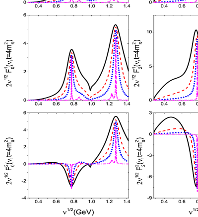
Figure 3: The $F^{I_{t}}_{n}(\nu,t)$ amplitudes for different values of $N_{C}$, see Eq. (13). Since $\int d\nu F^{I_{t}}_{n}(\nu,t)=\int d\sqrt{\nu}~{}2\sqrt{\nu}F^{I_{t}}_{n}(\nu,t)$, we plot $2\sqrt{\nu}F^{I_{t}}_{n}(\nu,t=4M_{\pi}^{2})$ here.

From Fig. 3 one notices that when $n$ is large and $N_{C}$ is not too large, the low energy amplitudes (including the $\sigma$), and the $\rho$ have much larger contributions, while the $f_{2}(1270)$ contributes most at $n=0$. Only in the $I_{t}=2$ amplitude the contribution of the $\rho$ is negative, which will cancel other contributions such as from the $\sigma$ in the low energy region and from the $f_{2}(1270)$ in the high energy region. This makes sure that $F^{I_{t}=2}_{n}(\nu,t)$ is super-convergent, being much smaller than the corresponding function for $I_{t}=0$ or $I_{t}=1$. Note that resonances/Regge exchanges are built from $q\bar{q}$ and multi-quark contributions. When $N_{C}$ is large, the pole of the $\bar{q}q$ state will fall down to the real axis on the $s$-plane (zero width), while the multi-quark component will disappear. Consequently, the $I_{s/t}=2$ amplitude is super-convergent at large $N_{C}$ as it does not contain any resonances or Regge poles. Also the ratio of the $I_{t}=1$ FESR compared to that of $I_{t}=0$ should be 2/3 in the large $N_{C}$ limit. These are analyzed in MRP11 within U$\chi$PT and we will check them with our method to generate the $N_{C}$-dependence in what follows.

Further, it is helpful to use the definition

$$F^{II^{\prime}}_{n}(t)=\frac{\int_{\nu_{min}}^{\nu_{max}}d\nu F^{I_{t}}_{n}(\nu,t)}{\int_{\nu_{min}}^{\nu_{max}}d\nu F^{I^{\prime}_{t}}_{n}(\nu,t)}\,.$$ (13)

As discussed before, semi-local duality means that $F^{10}_{n}(t)$ should be 2/3, and $F^{21,20}_{n}(t)$ be rather small. The values of these FESR for different values of $N_{C}$ are given in Tab. 3. For convenience, we plot $F^{10}_{n}(t)$ and $F^{21}_{n}(t)$ by tuning $N_{C}$ up to $N_{C}=180$, see Fig. 4.

Following Dai:2017uao , we simply assume that the whole contribution of the $N_{C}^{-2}$ corrections is roughly one third of that of $N_{C}^{-1}$, while the correlation between each polynomial is not discussed, despite the fact that the first two terms of the polynomials are fixed by the scattering lengths and slope parameters. In principal, the complete separated $N_{C}^{-2}$ dependence of each polynomial in Eq. (5) could be obtained by matching with $\chi PT$, if $\chi PT$ is calculated up to higher orders. However, this is not yet available. One certainly needs a more careful analysis of the $N_{C}^{-2}$ corrections. These higher-order $N_{C}$ corrections contribute most to the uncertainties at large $N_{C}$, estimated by randomly choosing $2/N_{C}+3/N_{C}^{2}$ and/or $4/N_{C}-3/N_{C}^{2}$ to replace $3/N_{C}$ in Eqs. (4,5) for each partial wave. The other contributions to the uncertainties are the higher partial waves, for instance the $IJ=13$ wave, whose amplitude has been given in KPY , and the systematic uncertainties from different solutions of the scattering amplitudes. The combination of all the three parts are collected as the total uncertainties, see Tab. 3 for $N_{C}=3,6,12,120$. The uncertainties are also shown as error bars in Fig. 4. We note that the uncertainty of the FESR increases as $N_{C}$ increases. See e.g. $F^{10,21}_{2}(4M_{\pi}^{2})$ in Tab. 3, with the upper limit $\nu_{max}=2$ GeV². This is because the uncertainty given by higher-order $N_{C}$ corrections is important. Besides, the uncertainty of the $F^{21}_{n}(t)$ is larger than that of $F^{10}_{n}(t)$. The reason is that the cancellation happens at $I_{t}=2$ and they are more sensitive to the relative difference of each partial waves. The uncertainty coming from the upper limit $\nu_{max}=1$ GeV² is smaller than that of $\nu_{max}=2$ GeV², this is caused by the important D-waves. We will discuss this later.

	n	$N_{C}$	$\nu_{max}=1$ GeV2		$\nu_{max}=2$ GeV2
			$t=4M_{\pi}^{2}$	$t=0$	$t=4M_{\pi}^{2}$	$t=0$
$F_{n}^{10}$	0	3	$0.50(2)$	$0.49(2)$	$0.56(5)$	$0.53(5)$
		6	$0.54(2)$	$0.55(2)$	$0.68(6)$	$0.67(5)$
		12	$0.57(2)$	$0.58(2)$	$0.75(6)$	$0.74(6)$
		120	$0.59(3)$	$0.61(3)$	$0.81(6)$	$0.82(6)$
	1	3	$0.51(2)$	$0.51(2)$	$0.55(3)$	$0.53(3)$
		6	$0.55(2)$	$0.56(2)$	$0.63(3)$	$0.62(3)$
		12	$0.56(2)$	$0.58(2)$	$0.67(3)$	$0.67(3)$
		120	$0.58(3)$	$0.60(3)$	$0.71(4)$	$0.72(3)$
	2	3	$0.54(2)$	$0.56(2)$	$0.55(2)$	$0.55(2)$
		6	$0.56(2)$	$0.58(2)$	$0.60(2)$	$0.60(2)$
		12	$0.57(2)$	$0.59(2)$	$0.62(2)$	$0.63(2)$
		120	$0.57(4)$	$0.58(4)$	$0.63(4)$	$0.65(3)$
	3	3	$0.58(2)$	$0.63(2)$	$0.58(2)$	$0.63(2)$
		6	$0.59(2)$	$0.62(2)$	$0.60(2)$	$0.63(2)$
		12	$0.58(2)$	$0.61(2)$	$0.60(2)$	$0.62(2)$
		120	$0.56(4)$	$0.57(4)$	$0.59(4)$	$0.60(3)$
$F_{n}^{21}$	0	3	$-0.41(2)$	$-0.30(2)$	$0.46(5)$	$0.50(5)$
		6	$-0.40(7)$	$-0.29(8)$	$0.50(11)$	$0.53(13)$
		12	$-0.39(11)$	$-0.27(12)$	$0.53(14)$	$0.56(17)$
		120	$-0.37(14)$	$-0.26(14)$	$0.56(14)$	$0.59(14)$
	1	3	$-0.33(2)$	$-0.18(2)$	$0.17(2)$	$0.24(2)$
		6	$-0.36(8)$	$-0.22(9)$	$0.19(11)$	$0.25(12)$
		12	$-0.39(12)$	$-0.26(13)$	$0.20(15)$	$0.25(18)$
		120	$-0.45(15)$	$-0.34(15)$	$0.22(15)$	$0.26(16)$
	2	3	$-0.13(2)$	$0.13(2)$	$0.05(2)$	$0.24(2)$
		6	$-0.24(7)$	$-0.04(9)$	$-0.00(10)$	$0.13(11)$
		12	$-0.34(10)$	$-0.18(12)$	$-0.05(14)$	$0.05(16)$
		120	$-0.51(12)$	$-0.41(16)$	$-0.13(16)$	$-0.07(15)$
	3	3	$0.20(2)$	$0.61(2)$	$0.24(2)$	$0.62(2)$
		6	$0.01(7)$	$0.37(9)$	$0.07(10)$	$0.40(11)$
		12	$-0.19(9)$	$0.11(12)$	$-0.09(13)$	$0.17(17)$
		120	$-0.55(11)$	$-0.43(15)$	$-0.37(17)$	$-0.28(17)$

Table 3: Duality by tuning $N_{C}$, given here for $N_{C}=3$, $6$, $12$, $120$.

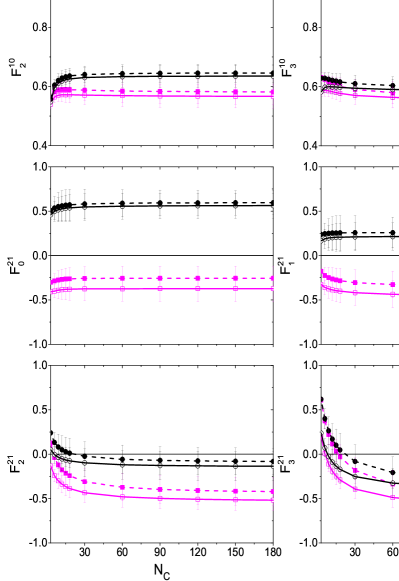
Figure 4: Duality by varying $N_{C}$ from 3 to a large number, in the order of $N_{C}=3$, $6$, $9$, $12$, $15$, $18$, $30$, $60$, $90$, $120$, $150$ and $180$.

The results are quite different when the upper limit is chosen to be 1 GeV² or 2 GeV², especially in terms of $n=0,1$. As an example, for $F^{21}_{0,1}(t)$ the sign of the results with these two upper limits are even opposite. For $n=2,3$, the differences are still distinct but smaller. This is consistent with our analysis that the $IJ=02$ wave contributes a lot in the resonance region at small $n$ (0 or 1). In Fig. 3, the peaks of the $f_{2}(1270)$ in $F^{I}_{0}(\nu,t)$ are much larger than those in $F^{I}_{2}(\nu,t)$. While at large $n$ ($n=2,3$), the contribution of the $IJ=02$ wave in the resonance region is still important but smaller. Therefore, we consider the upper limit of 2 GeV² as the optimal choice.

The change of the results with different $n$ of $F^{10}_{n}(t)$ is smaller than that of $F^{21}_{n}(t)$ in the large $N_{C}$ case. For example, with upper limit $\nu_{max}=2$ GeV² and $N_{C}=120$, the difference between $F^{10}_{0}(4M_{\pi}^{2})$ and $F^{10}_{3}(4M_{\pi}^{2})$ is 0.22, while the difference between $F^{21}_{0}(4M_{\pi}^{2})$ and $F^{21}_{3}(4M_{\pi}^{2})$ is 0.93! The reason is that the contribution from the $\rho$ dominates both amplitudes in $I_{t}=0$ and $I_{t}=1$ below 1 GeV, and the relative sign between different resonances ($\rho$,$f_{2}(1270)$ etc.) are positive, while in $I_{t}=2$ the relative sign is negative, see also Eq. (9). This can be checked in Fig. 3, by comparing the lines of $2\sqrt{\nu}F^{0}_{2}(\nu,t=4M_{\pi}^{2})$ and $2\sqrt{\nu}F^{1}_{2}(\nu,t=4M_{\pi}^{2})$.

At large $N_{C}$, none of the absolute values of $F^{21}_{n}(t)$ is larger than 0.6, and all $F^{10}_{n}(t)$ are distributed in the region [0.6,0.8]. For $n=2$, with the upper limit 2 GeV² and $N_{C}=180$, both $F^{10}_{2}(4M_{\pi}^{2})=0.64\pm 0.04$ and $F^{21}_{2}(4M_{\pi}^{2})=-0.14\pm 0.16$ are very close to the expected value, $2/3$ and 0, respectively. Similarly, we have $F^{10}_{2}(0)=0.65\pm 0.03$ and $F^{21}_{2}(0)=-0.08\pm 0.15$, even a bit closer. We note that the two kinds of results, with $t=0$ or $t=4M_{\pi}^{2}$, are rather similar to each other. We thus only discuss the case with $t=4M_{\pi}^{2}$ in the next sections. For $n=1,3$ the situation is not so good, but the values are still fairly close to the expected values. For $n=1$ we have $F^{10}_{1}(4M_{\pi}^{2})=0.72\pm 0.04$ and $F^{21}_{1}(4M_{\pi}^{2})=0.22\pm 0.15$, and for $n=3$ we find $F^{10}_{3}(4M_{\pi}^{2})=0.59\pm 0.04$ and $F^{21}_{3}(4M_{\pi}^{2})=-0.38\pm 0.17$. The $F^{21}_{n}(0,4M_{\pi}^{2})$ at large $N_{C}$ indicates that the $f_{2}(1270)$ (also the $f_{0}(980)$ and the $f_{0}(1370)$) will cancel the contribution of the $\rho(770)$ most at $n=2$. By increasing/decreasing $n$ the cancellation is less precise, as the masses of these resonances are different. By dividing with $\nu^{n}$ the contribution of the $\rho$ and that of the $f_{2}(1270)/f_{0}(980)$ are mismatched, especially around $\nu=M_{R}^{2}$. As discussed in the earlier sections, $n=1-3$, especially $n=2,3$, are the most valuable cases to check the semi-local duality, one thus concludes that the results support that the semi-local duality is fulfilled well up to $N_{C}=180$. There are some other points that could be interesting. Almost all the lines in Fig.4 are increased/decreased a bit strongly from $N_{C}=3$ to $N_{C}=30$. One of the reasons is that the physical amplitudes are not as simple as that just represented by one or two Breit-Wigner resonances. Other components, such as multi-quark components and other background, will also contribute a lot when $N_{C}$ is not far away from 3. Such variation of the lines of $F^{21}_{n=2,3}(t)$ is more obvious than that of $F^{10}_{n=2,3}(t)$, where the latter is within $1/3$ level. This is because the former has a strong cancellation between isospin 0 and 1 waves in the s-channel, as shown in Eqs. (9,10). The complex $N_{C}$ relations of scalars enlarge the variation. We also notice that the lines are very flat in the region of $N_{C}\in[100,180]$. It is thus natural to infer that they will stay flat for larger $N_{C}$. This suggests that the semi-local duality will hold in the large $N_{C}$ limit.

To estimate the contribution of each resonance at large $N_{C}$, we perform the following calculations:

• Case A: The amplitudes of the $IJ=00$ wave in the region of $\sqrt{s}\leq 0.75$ GeV have been set to zero. In this case the main contribution of $f_{0}(500)$ is removed.

• Case B: Similar to Case A, the amplitudes of the $IJ=00$ wave in the region of $\sqrt{s}\in[0.81,0.91]$ GeV have been set to zero. The $f_{0}(980)$ is removed in the large $N_{C}$ limit.

• Case C: Similar to Case A, the amplitudes of the $IJ=00$ wave in the region of $\sqrt{s}\in[1.13,1.33]$ GeV have been set to zero. The $f_{0}(1370)$ is removed in the large $N_{C}$ limit.

• Case D: Similar to Case A, the amplitudes of the $IJ=02$ wave in the region of $\sqrt{s}\in[1.15,1.4]$ GeV have been set to zero. The contribution of the $f_{2}(1270)$ is removed.

• Case E: Only the upper limit is changed to $\nu_{max}=4$ GeV², where the possible contribution of heavier resonances, like $\rho(1450)$, $\rho(1710)$ etc. is included.

The results are shown in Tab. 4. For Cases A, D and E, the results by tuning $N_{C}$ are plotted as magenta, black, and cyan lines, respectively, in Fig. 5. For Cases B and C, we can not extract the contributions of the relevant resonances except at large $N_{C}$, as there is no obvious peak for $f_{0}(980)$ and $f_{0}(1370)$ around $N_{C}=3$. Therefore, we only show the results at $N_{C}=180$, see Tab. 4.

Case	$F^{10}_{2}(t)$		$F^{21}_{2}(t)$
	$t=4M_{\pi}^{2}$	$t=0$	$t=4M_{\pi}^{2}$	$t=0$
O	$0.64(5)$	$0.65(4)$	$-0.14(16)$	$-0.06(15)$
A	$0.63(7)$	$0.64(7)$	$-0.15(20)$	$-0.10(19)$
B	$0.59(8)$	$0.59(7)$	$-0.36(20)$	$-0.34(19)$
C	$0.62(8)$	$0.63(7)$	$-0.23(20)$	$-0.19(19)$
D	$0.59(3)$	$0.61(3)$	$-0.37(15)$	$-0.27(16)$
E	$0.63(8)$	$0.65(7)$	$-0.13(20)$	$-0.08(19)$

Table 4: Duality for the different Cases at $N_{C}=180$ discussed in the text. Note that Case O is the original result shown in Fig. 4.

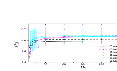
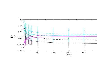
Figure 5: Duality for the different cases defined in the text. We vary $N_{C}$ from 3 to a large number, in the order of $N_{C}=3$, $6$, $9$, $12$, $15$, $18$, $30$, $60$, $90$, $120$, $150$ and $180$.

For Case A, we have $F^{10}_{2}(4M_{\pi}^{2})=0.63\pm 0.07$ and $F^{21}_{2}(4M_{\pi}^{2})=-0.15\pm 0.20$ at $N_{C}=180$. These satisfy the semi-local duality well. At $N_{C}=3$, we have $F^{21}_{2}(4M_{\pi}^{2})=-0.36\pm 0.12$. It changes a lot comparing to the original result, cf. Tab. 3. It confirms that the $\sigma$ contribution is not ignorable at $N_{C}=3$, while it is smaller and irrelevant in the large $N_{C}$ limit. The cancellation does not happen between the $\sigma$ and $\rho(770)$ in the large $N_{C}$ limit. This also suggests that $\sigma$ is dominated by the non-$\bar{q}q$ structure components.

It is worth to point out that in Ref. Guo:2012yt , where U$\chi$PT based on the N/D method has been applied to the meson-meson scattering of the $U(3)$ nonet, the $f_{0}(980)$ contribution can not be ignored to cancel the contribution of $\rho$. In contrast, in Ref.MRP11 , where U$\chi$PT is realized by inverse amplitude method, the $f_{0}(980)$ is irrelevant and a sub-dominant $\bar{q}q$ component is needed for the cancellation. For the $f_{0}(1370)$, both of these two works agree as the resonance does not contribute a lot at large $N_{C}$. In our case, the two resonances behave as ‘peaks’ around 0.85 GeV and 1.23 GeV at large $N_{C}$, respectively. This supports their possible inner $\bar{q}q$ component, resulting in a possible contribution to cancel the $\rho$ in $F^{21}_{n}(t)$. We find numerically for Case B, where the contribution of the $f_{0}(980)$ has been removed at large $N_{C}$, that $F^{10}_{2}(4M_{\pi}^{2})=0.59\pm 0.08$ and $F^{21}_{2}(4M_{\pi}^{2})=-0.36\pm 0.20$ at $N_{C}=180$. Comparing to the original results (Case O), the value of $F^{10}_{2}(0,4M_{\pi}^{2})$ change a bit, and that of $F^{21}_{2}(0,4M_{\pi}^{2})$ change a lot. Thus, the contribution of the $f_{0}(980)$ at large $N_{C}$ can not be ignored. For Case C, by removing the $f_{0}(1370)$ at large $N_{C}$, the change is smaller than that of Case B but still distinct, see Tab. 4. This implies that the $f_{0}(980)$ and the $f_{0}(1370)$ have a significant $\bar{q}q$ component and they will partly cancel the contribution of the $\rho$.

In Case D the $f_{2}(1270)$ has been removed. One finds $F^{10}_{2}(4M_{\pi}^{2})=0.59\pm 0.03$ and $F^{21}_{2}(4M_{\pi}^{2})=-0.37\pm 0.15$ at $N_{C}=180$. The $f_{2}(1270)$ contribution is rather important to cancel that of the $\rho$, just as expected. The results of Case D is rather close to that of the $f_{0}(980)$ at large $N_{C}$, implying the same important contribution of the $f_{0}(980)$ as the $f_{2}(1270)$. In case E we consider the FESR with the upper limit $\nu_{max}=4$ GeV². The results at $N_{C}=180$ are almost the same as that of Case O. This supports the view that the $\rho(1450)$ as well as other heavier resonances do not have a large effect. In Fig. 5 one clearly sees that in Case D the $F^{10}_{2}(t)$ and $F^{10}_{2}(t)$ deviate much more from the expected values than that in Cases A and E. This confirms that the $f_{2}(1270)$ has a much larger effect than the $f_{0}(500)$ and heavier resonances such as the $\rho(1450)$.

IV Summary

In this paper we have studied the semi-local duality for large $N_{C}$. The isospin-2 $\pi\pi$ scattering amplitudes with final-state interactions are constructed in a model-independent way and fit to the data. Comparing with the amplitudes of $\chi$PT, we generate the $N_{C}$-dependence of the amplitudes. With this $N_{C}$-dependence the semi-local duality in terms of finite energy sum rules is tested. Our results show that the semi-local duality is satisfied well in the large $N_{C}$ limit, at least up to $N_{C}=180$. This study confirms that the method of generating the $N_{C}$ dependence proposed in Ref. Dai:2017uao is reliable. At large $N_{C}$, the contributions of the $f_{2}(1270)$ and the $f_{0}(980)$ are important to cancel that of the $\rho(770)$, the latter is consistent with what has been found in Ref. Guo:2012yt . Also the $f_{0}(1370)$ contributes significantly to the cancellation. In contrast, the $f_{0}(500)$ (or $\sigma$) has a large effect for $N_{C}=3$ and a small effect at large $N_{C}$. These support the $\bar{q}q$ component in the $f_{0}(980)$ and the $f_{0}(1370)$, but not for the $\sigma$ as required in Ref. MRP11 .

References

- (1) L. Y. Dai and U.-G. Meißner, Phys. Lett. B 783 (2018) 294 arXiv: 1706.10123 [hep-ph].
- (2) G. ’t Hooft, Nucl. Phys. B72, 461 (1974).
- (3) G. ’t Hooft, Nucl.Phys. B75, 461 (1974).
- (4) J.R. Pelaez, Phys. Rev. Lett. 92, 102001 (2004). arXiv: 0309292 [hep-ph].
- (5) J.R. Pelaez and G. Rios, Phys. Rev. Lett. 97, 242002 (2006). arXiv: 0610397 [hep-ph].
- (6) Z.X. Sun et al., Mod. Phys. Lett. A22, 711 (2007). arXiv: 0503195 [hep-ph].
- (7) J.R. Pelaez, M.R. Pennington, J. Ruiz de Elvira and D.J. Wilson, Phys. Rev. D 84, 096006 (2011), arXiv: 1009.6204 [hep-ph];
- (8) L.Y. Dai, X.G. Wang and H.Q. Zheng, Commun. Theor. Phys. 57, 841 (2012), arXiv: 1108.1451 [hep-ph]; Commun. Theor. Phys. 58, 410 (2012), arXiv: 1206.5481 [hep-ph].
- (9) G. Veneziano, Nuovo Cim. A 57, 190 (1968).
- (10) R. Dolen, D. Horn and C. Schmid, Phys. Rev. Lett. 19, 402 (1967).
- (11) R. Dolen, D. Horn and C. Schmid, Phys. Rev. 166, 1768 (1968).
- (12) C. Schmid, Phys. Rev. Lett. 20, 628 (1968).
- (13) C. Schmid, Phys. Rev. Lett. 20, 689 (1968).
- (14) K. Shiga, K. Kinoshita and F. Toyoda, Nucl. Phys. B 24, 490 (1970).
- (15) Z. H. Guo, J. A. Oller and J. Ruiz de Elvira, Phys. Rev. D 86, 054006 (2012), arXiv: 1206.4163 [hep-ph].
- (16) H. q. Zheng, Int. J. Mod. Phys. A 20, 1981 (2005), arXiv: hep-ph/0411025.
- (17) K.L. Au, D. Morgan and M.R. Pennington, Phys. Rev. D 35 1633 (1987); D. Morgan and M.R. Pennington, Phys. Rev. D 48 1185 (1993).
- (18) U.-G. Meißner, Comments Nucl. Part. Phys. 20, 119 (1991).
- (19) Z.H. Guo and J. A. Oller, Phys. Rev. D 84 034005 (2011), arXiv: 1104.2849 [hep-ph].
- (20) L. Y. Dai, M. Shi, G. Y. Tang and H. Q. Zheng, Phys. Rev. D 92, no. 1, 014020 (2015), arXiv: 1206.6911 [hep-ph].
- (21) C. Garc a-Recio, L. S. Geng, J. Nieves, L. L. Salcedo, E. Wang and J. J. Xie, Phys. Rev. D 87, no. 9, 096006 (2013) arXiv: 1304.1021 [hep-ph].
- (22) X. W. Kang, J. Haidenbauer and U.-G. Meißner, JHEP 1402, 113 (2014) arXiv: 1311.1658 [hep-ph].
- (23) X.W. Kang, B. Kubis, C. Hanhart and U.-G. Meißner, Phys. Rev. D 89 053015 (2014), arXiv: 1312.1193 [hep-ph].
- (24) Y.H. Chen, J. T. Daub, F.K. Guo, B. Kubis, Ulf-G. Meißner and B.S. Zou, Phys. Rev. D 93 034030 (2015), arXiv: 1512.03583 [hep-ph].
- (25) Raul A. Briceno, Jozef J. Dudek, Robert G. Edwards, David J. Wilson, Phys. Rev. Lett. 118, 022002, (2017). arXiv: 1607.05900 [hep-ph].
- (26) G. Colangelo, S. Lanz, H. Leutwyler and E. Passemar, Phys. Rev. Lett. 118, no.2, 022001 (2017), arXiv: 1610.03494 [hep-ph].
- (27) C. Hanhart, S. Holz, B. Kubis, A. Kupść, A. Wirzba and C. W. Xiao, Eur. Phys. J. C 77, no. 2, 98 (2017), Erratum: [Eur. Phys. J. C 78, no. 6, 450 (2018)], arXiv: 1611.09359 [hep-ph].
- (28) L. Y. Dai, J. Haidenbauer and U.-G. Meißner, JHEP 1707, 078 (2017) [arXiv:1702.02065 [nucl-th]]. arXiv: 1702.02065 [nucl-th].
- (29) H. Y. Cheng and X. W. Kang, Eur. Phys. J. C 77, no. 9, 587 (2017) Erratum: [Eur. Phys. J. C 77, no. 12, 863 (2017)] [arXiv:1707.02851 [hep-ph]]. arXiv: 1707.02851 [hep-ph].
- (30) R. Omnès, Nuovo Cim.8, 316 (1958).
- (31) L.Y. Dai and M.R. Pennington, Phys. Lett. B736 11 (2014), arXiv: 1403.7514 [hep-ph]; Phys. Rev. D 90 036004 (2014), arXiv: 1404.7524 [hep-ph].
- (32) L. Y. Dai, V. Mathieu, E. Passemar, M. R. Pennington and A. Szczepaniak, in preparation.
- (33) N. B. Durusoy, M. Baubillier, R. George, M. Goldberg and A. M. Touchard, Phys. Lett. B45 (1973) 517;
- (34) R. García- Martín, R. Kamiński, J. R. Peláez, J. Ruiz de Elvira, and F. J. Ynduráin, Phys. Rev. D 83 074004 (2011), arXiv: 1102.2183 [hep-ph].
- (35) M.M. Nagels et al. , Nucl. Phys. B147 189 (1979);
- (36) J. Gasser, H. Leutwyler, Ann. Phys. (NY) 158 142 (1984).
- (37) J. Gasser, H. Leutwyler, Nucl. Phys. B250 465 (1985).
- (38) J. Bijnens, G. Colangelo and J. Gasser, Nucl. Phys. B427 427 (1994).
- (39) A. Gomez Nicola, J. R. Pelaez, Phys. Rev. D 65 054009 (2002). arXiv: 0109056 [hep-ph].
- (40) L. Y. Dai, X. W. Kang, U.-G. Meißner, X. Y. Song and D. L. Yao, Phys. Rev. D 97 036012 (2018), arXiv: 1712.02119 [hep-ph].
- (41) R. Kaminski, Phys. Rev. D 83 (2011) 076008 [arXiv:1103.0882 [hep-ph]]. arXiv: 1103.0882 [hep-ph].
- (42) Z. H. Guo, J. J. Sanz Cillero and H. Q. Zheng, JHEP 0706, 030 (2007), arXiv:hep-ph/0701232.
- (43) J. T. Londergan, J. Nebreda, J. R. Pelaez and A. Szczepaniak, Phys. Lett. B 729, 9 (2014), arXiv: 1311.7552 [hep-ph].
- (44) S. Weinberg, Phys. Rev. Lett. 110 261601 (2013), arXiv: 1303.0342 [hep-ph].
- (45) M. Knecht and S. Peris, Phys. Rev. D 88, 036016 (2013), arXiv: 1307.1273 [hep-ph].
- (46) T. Ledwig, J. Nieves, A. Pich, E.R. Arriola, and J. Ruiz de Elvira, Phys. Rev. D 90 114020 (2014). arXiv: 1407.3750 [hep-lat].
- (47) J. Nieves and E. Ruiz Arriola, Phys. Lett. B 679, 449 (2009), arXiv:0904.4590 [hep-ph].