$0\nu\beta\beta$ nuclear matrix elements, neutrino potentials and $\mathrm{SU}(4)$ symmetry

Abstract

Intimate relation between the Gamow-Teller part of the matrix element $M^{0\nu}_{\mathrm{GT}}$ and the $2\nu\beta\beta$ closure matrix element $M^{2\nu}_{\mathrm{cl}}$ is explained and explored. If the corresponding radial dependence $C^{2\nu}_{\mathrm{cl}}(r)$ would be known, $M^{0\nu}$ corresponding to any mechanism responsible for the $0\nu\beta\beta$ decay can be obtained as a simple integral. However, the $M^{2\nu}_{\mathrm{cl}}$ values sensitively depend on the properties of higher lying $1^{+}$ states in the intermediate odd-odd nuclei. We show that the $\beta^{-}$ and $\beta^{+}$ amplitudes of such states typically have opposite relative signs, and their contributions reduce severally the $M^{2\nu}_{\mathrm{cl}}$ values. Vanishing values of $M^{2\nu}_{\mathrm{cl}}$ are signs of a partial restoration of the spin-isospin $\mathrm{SU}(4)$ symmetry. We suggest that demanding that $M^{2\nu}_{\mathrm{cl}}$ = 0 is a sensible way, within the method of the Quasi-particle Random Phase Approximation (QRPA), of determining the amount of renormalization of isoscalar particle-particle interaction strength $g^{T=0}_{pp}$. Using such prescription, the matrix elements $M^{0\nu}$ are evaluated; their values are not very different ($\leq$ 20%) from the usual QRPA values when $g^{T=0}_{pp}$ is related to the known $2\nu\beta\beta$ half-lives.

I Introduction

Neutrinos are the only known elementary particles that may be Majorana fermions, i.e., identical with their antiparticles. They are also very light, suggesting that the origin of their mass could be different from the origin of mass of all other fermions that are much heavier and charged, supporting such hypothesis. Study of the neutrinoless double beta decay ($0\nu\beta\beta$), the transition among certain even-even nuclei when two neutrons bound in the ground state are transformed into two bound protons and two electrons with nothing else emitted, is the most straightforward test whether neutrino are indeed Majorana fermions. Obviously, observing such decay would mean that the Lepton Number is not a conserved quantity as required by the Standard Model.

There is an intense worldwide effort to search for the $0\nu\beta\beta$ decay. No signal has been observed so far, but impressive half-life limits of more than $10^{25-26}$ years have been achieved in several experiments on several target nuclei. Larger, and even more sophisticated experiments are developed and/or planned. Search for the $0\nu\beta\beta$ decay is at the forefront of the present day nuclear and particle physics.

While observation of the $0\nu\beta\beta$ decay would constitute a proof that neutrinos are massive Majorana fermions SV , it is obviously desirable to be able to relate the observed half-life to some ‘beyond the Standard Model’ particle physics theory. To do that, however, requires understanding of the nuclear structure issues involved in the $(Z,A)_{\rm g.s.}\rightarrow(Z+2,A)_{\rm g.s.}+2e^{-}$ transition. The problem at hand is the evaluation of the corresponding nuclear matrix elements. This is a long standing issue, with a plethora of papers devoted to this subject. Recent review EM summarizes the present status.

Here we explore in more detail the relation between the nuclear matrix elements of the $0\nu\beta\beta$ decay and of the allowed and experimentally observed $2\nu\beta\beta$ decay, treated however in the closure approximation. This is a continuation and expansion of the earlier paper SHFV . We concentrate primarily on the expression of these matrix elements as functions of the relative distance $r$ between the two neutrons that are transformed into the two protons in the $\beta\beta$ decay. Naturally, we keep in mind that the closure approximation is not applicable for the $2\nu\beta\beta$ mode of the $\beta\beta$ decay.

The paper is organized as follows. After this Introduction, in the next section the so-called neutrino potentials are described, and their dependence on the distance $r$ between the decaying neutrons. Next, the two neutrino ($2\nu\beta\beta$) decay matrix elements in closure approximation and their relation to the $0\nu\beta\beta$ decay matrix elements are discussed. In the following section advantages of the $LS$ coupling scheme are described and symmetry consideration are applied. In section V the $0\nu\beta\beta$ matrix elements, based on previous considerations, are evaluated and their values are compared to the previously published ones. The partial restoration of the spin-isospin symmetry $\mathrm{SU}(4)$ is also discussed there. Finally, the Summary section concludes the paper.

Very generally, the observable $0\nu\beta\beta$ decay rate is expressed as a product of three factors

$$\frac{1}{T_{1/2}}=G^{0\nu}(Z,E_{0})(M^{0\nu})^{2}\phi^{2}~{},$$ (1)

where $G^{0\nu}(Z,E_{0})$ is the calculable phase space factor that in this case also includes all necessary fundamental constants, and that depends on the nuclear charge $Z$ and on the decay endpoint energy $E_{0}$. $M^{0\nu}$ is the nuclear matrix element that depends, among other things, on the particle physics mechanism responsible for the the $0\nu\beta\beta$ decay, as does the phase space factor $G^{0\nu}(Z,E_{0})$. And by $\phi$ we symbolically denote the corresponding particle physics parameter that we would like to extract from experiment.

For any mechanism responsible for the decay, the matrix element $M^{0\nu}$ consists of three parts, Fermi, Gamow-Teller and Tensor

$$M^{0\nu}=M^{0\nu}_{\mathrm{GT}}-\frac{M^{0\nu}_{\mathrm{F}}}{g_{\rm A}^{2}}+M^{0\nu}_{\rm T}~{},$$ (2)

where $g_{\rm A}$ is the nucleon axial current coupling constant. And, in turn, the $\mathrm{GT}$ part, evaluated in the closure approximation, is

$$M^{0\nu}_{\mathrm{GT}}=\langle f|\sum_{k,l}\vec{\sigma}_{k}\cdot\vec{\sigma}_{l}\tau^{+}_{k}\tau^{+}_{l}H_{\mathrm{GT}}(r_{kl},\bar{E})|i\rangle~{}.$$ (3)

The Fermi part, again in closure, is given by an analogous formula

$$M^{0\nu}_{\mathrm{F}}=\langle f|\sum_{k,l}\tau^{+}_{k}\tau^{+}_{l}H_{\mathrm{F}}(r_{kl},\bar{E})|i\rangle~{}.$$ (4)

And the tensor part is

$$M^{0\nu}_{T}=\langle f|\sum_{k,l}[3(\vec{\sigma}_{k}\cdot\vec{\hat{r}}_{kl})(\vec{\sigma}_{l}\cdot\vec{\hat{r}}_{kl})-\vec{\sigma}_{k}\cdot\vec{\sigma}_{l}]\tau^{+}_{k}\tau^{+}_{l}H_{\rm T}(r_{kl},\bar{E})|i\rangle~{}.$$ (5)

Here $|i\rangle,|f\rangle$ are the ground state wave functions of the initial and final nuclei. $H_{\mathrm{GT}}(r_{ij},\bar{E})$, $H_{\mathrm{F}}(r_{ij},\bar{E})$ and $H_{\rm T}(r_{ij},\bar{E})$ are the “neutrino potentials” that depend on the relative distance $r_{ij}$ of the two nucleons. The sum is over all nucleons in the nucleus. The dependence on the average nuclear excitation energy $\bar{E}$ is usually quite weak. We discuss the validity of the closure approximation for the $0\nu\beta\beta$ mode in the next section.

II Neutrino potentials

Neutrino potentials in eqs. (3), (4) and (5) are typically defined as integrals over the momentum transfer $q$. They cannot be expressed by an analytic formula as functions of the internucleon distance $r_{ij}$. In the following we will concentrate on the “standard” scenario, where the $0\nu\beta\beta$ decay is associated with the exchange of light Majorana neutrinos. In that case the particle parameter $\phi$ in eq. (1) is the effective Majorana neutrino mass

$$m_{\beta\beta}=\left|\sum_{i=1}^{3}|U_{ei}|^{2}e^{{\rm i}\alpha_{i}}m_{i}\right|,$$ (6)

where $U_{ei}$ are the, generally complex, matrix elements of the first row of the PMNS neutrino mixing matrix with phases $\alpha_{i}$, and $m_{i}$ are the masses of the corresponding mass eigenstates neutrinos. The present values of the mixing angles and mass squared differences $\Delta m_{ij}^{2}$ are listed e.g. in the Review of Particle Properties PDG17 .

For this mechanism, the dimensionless neutrino potential for the $K=\mathrm{GT},\rm F$ and $\rm T$ parts is

$$H_{K}(r_{12},\bar{E}) = f^{2}_{\rm src}(r_{12})\times$$

$$\frac{2}{\pi g_{\rm A}^{2}}{R}\int_{0}^{\infty}~{}f_{K}(qr_{12})~{}\frac{h_{K}(q^{2})qdq}{q+\bar{E}}\,.$$

here $R$ is the nuclear radius added to make the potential dimensionless. The functions $f_{\mathrm{F},\mathrm{GT}}(qr_{12})=j_{0}(qr_{12})$ and $f_{\rm T}(qr_{12})=-j_{2}(qr_{12})$ are spherical Bessel functions. The functions $h_{K}(q^{2})$ are defined in anatomy (see also SPVF ). The potentials depend rather weakly on average nuclear excitation energy $\bar{E}$. The function $f_{\rm src}(r_{12})$ represents the effect of two-nucleon short range correlations. In the following we use the $f_{\rm src}(r_{12})$ derived in Sim09 . The phase space factors for this mechanism are listed e.g. in KI12 .

However, the exchange of light Majorana neutrinos is not the only way $0\nu\beta\beta$ decay can occur. Many particle physics models that contain so far unobserved new particles at the $\sim\mathrm{TeV}$ mass scale also contain $\Delta L=2$ higher dimension operators that could lead to the $0\nu\beta\beta$ decay with a rate comparable to the rate associated with the light Majorana neutrino exchange. These models also explain why neutrinos are so light. Moreover, some of their predictions can be confirmed (or rejected) at the LHC or beyond. Examples of these models are the Left-Right Symmetric Model or the R-parity Violating Supersymmetry. In them, heavy ($M\gg M_{p}$, $M_{p}$ is the proton mass) particles are exchanged between the two neutrons that are transformed into the two protons. There is a large variety of neutrino potentials corresponding to such mechanisms of $0\nu\beta\beta$ decay. A list of them, and of the corresponding phase space factors, can be found e.g. in ref. HN17 . For a complete description of the $0\nu\beta\beta$ decay it would be, therefore, necessary to evaluate $\sim 20$ different nuclear matrix elements. We show below, how this task could be substantially simplified.

The matrix elements defined in the eqs. (3), (4) and (5) are evaluated in the closure approximation. In that case only the wave functions of the initial and final ground states are needed. The validity of this approximation can be tested in the Quasi-particle Random Phase Approximation (QRPA), where the summation over the intermediate states is easily implemented as done in Ref. SHFV . There it was shown that the closure approximation typically results in matrix elements that are at most 10% smaller than those obtained by explicitly summing over the intermediate virtual states. The dependence on the assumed average energy $\bar{E}$ is weak; it makes little difference if $\bar{E}$ is varied between 0 and 12 MeV. Similar conclusion was reached using the nuclear shell model (see Ref. SH and references therein).

Better insight into the structure of matrix elements can be gained by explicitly considering their dependence on the distance $r$ between the two neutrons that are transformed into two protons in the decay. Thus we define the function $C^{0\nu}_{\mathrm{GT}}(r)$ (and analogous ones for $M_{\mathrm{F}}$ and $M_{\rm T}$) as

$$C^{0\nu}_{\mathrm{GT}}(r)=\langle f|\sum_{k,l}\vec{\sigma}_{k}\cdot\vec{\sigma}_{l}\tau^{+}_{k}\tau^{+}_{l}\delta(r-r_{kl})H{{}_{\mathrm{GT}}}(r_{kl},\bar{E})|i\rangle~{}.$$ (8)

This function is, obviously, normalized as

$$M^{0\nu}_{\mathrm{GT}}=\int_{0}^{\infty}C^{0\nu}_{\mathrm{GT}}(r)dr~{}.$$ (9)

In other words, knowledge of $C^{0\nu}_{\mathrm{GT}}(r)$ makes the evaluation of $M^{0\nu}_{\mathrm{GT}}$ trivial. The function $C(r)$ was first introduced in Ref. anatomy .

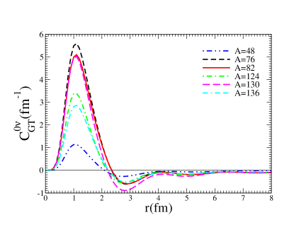
Figure 1: Functions $C^{0\nu}_{\mathrm{GT}}(r)$ evaluated in the QRPA for a number of $0\nu\beta\beta$ candidate nuclei.

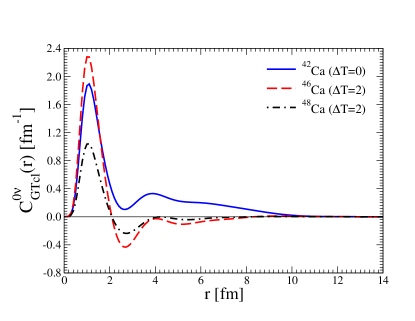
Figure 2: Functions $C^{0\nu}_{\mathrm{GT}}(r)$ evaluated in the QRPA for several Ca isotopes. ⁴⁸Ca is a real $\beta\beta$ decay candidate. It decays into ⁴⁸Ti and the isospin $T$ changes in the decay by two units ($\Delta T=2$). The other two Ca isotopes cannot $\beta\beta$ decay; nevertheless the corresponding matrix elements can be evaluated. The transition ⁴²Ca $\rightarrow^{42}$Ti connects mirror nuclei, the isospin does not change, $\Delta T=0$.

As one can see in Fig.1 the function $C^{0\nu}_{\mathrm{GT}}(r)$ consists primarily of a peak with the maximum at 1.0-1.2 fm and a node at 2-2.5 fm. The negative tail past this node contributes relatively little to the integral over $r$ and hence to the value of $M^{0\nu}_{\mathrm{GT}}$. The shape of the function $C^{0\nu}_{\mathrm{GT}}(r)$ is essentially the same for all $0\nu\beta\beta$ decay candidates. The magnitude of the matrix element $M^{0\nu}_{\mathrm{GT}}$ is determined, essentially, by the value of the peak maximum, which can be related, among other things, to the pairing properties of the involved nuclei.

This characteristic behavior of the function $C^{0\nu}_{\mathrm{GT}}(r)$ repeats itself when it is evaluated instead in the nuclear shell model; same peak, same node, little effect of the tail past the node XM9 . The same function was also evaluated in P17 for the hypothetical decay ¹⁰He $\rightarrow^{10}$Be using the ab initio variational Monte-Carlo method. The function $C^{0\nu}_{\mathrm{GT}}(r)$ has, again even in this case, qualitatively similar shape with a similar peak and same node, but the negative tail appears to be somewhat more pronounced. We might conclude that, at least qualitatively, the shape of $C^{0\nu}_{\mathrm{GT}}(r)$ is universal; it does not depend on the method used to calculate it, even though the methods mentioned here, QRPA, nuclear shell model, or the ab initio variational Monte-Carlo are vastly different in the way the ground state wave functions $|i\rangle$ and $|f\rangle$ are evaluated.

In all $\beta\beta$ decay candidate nuclei the isospin $T$ of the initial nucleus is different, by two units, from the isospin of the final nucleus; thus $\Delta T=2$. To study theoretically nuclear matrix element evaluation it is not necessary to consider only the $\beta\beta$ transitions allowed by the energy conservation rules. Thus, transitions within an isospin multiplet ($\Delta T=0$), such as ⁴²Ca $\rightarrow^{42}$Ti or ⁶He $\rightarrow^{6}$Be can be, and are, considered. The corresponding radial dependence $C^{0\nu}_{\mathrm{GT}}(r)$ is different in that case. There is no node, the function remain positive over the whole $r$ range. For QRPA this is illustrated in Fig. 2. Again, in the $\it ab~{}initio$ evaluation P17 for the hypothetical transition ⁶He $\rightarrow^{6}$Be that feature is there as well, even though the shape of the curve is rather different than for the ⁴²Ca case. The fact that the functions $C^{0\nu}_{\mathrm{GT}}(r)$ are quite different when $\Delta T=2$ and $\Delta T=0$ cases are considered, suggests that it is not obvious whether the experience obtained from the latter cases in light nuclei can be easily generalized to the decays of real $0\nu\beta\beta$ decay candidate nuclei which are all $\Delta T=2$.

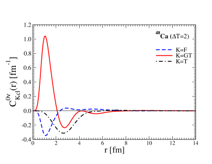
Figure 3: Functions $C^{0\nu}_{K}(r)$ evaluated in the QRPA for the Gamow-Teller (GT), Fermi (F) and Tensor (T) matrix elements for ⁴⁸Ca $0\nu\beta\beta$ decay.

The radial functions $C^{0\nu}_{\mathrm{F}}(r)$ and $C^{0\nu}_{\mathrm{T}}(r)$ corresponding to the Fermi, eq. (4), and Tensor, eq. (5), matrix elements are obtained in an analogous way. A typical example is shown in Fig. 3. The function $C^{0\nu}_{\mathrm{F}}(r)$ has very similar shape as $C^{0\nu}_{\mathrm{GT}}(r)$, but has opposite sign (see, however the sign in eq. (2)). The relation of $C^{0\nu}_{\mathrm{F}}(r)$ and $C^{0\nu}_{\mathrm{GT}}(r)$ will be discussed in detail in section IV. Notice that the correlation function $C^{0\nu}_{\mathrm{T}}(r)$ corresponding to the tensor matrix element does not share the properties of the main peak.

III $2\nu\beta\beta$ matrix elements in closure approximation

It would be clearly desirable to find a relation between the $0\nu\beta\beta$ matrix elements and another quantity that does not depend on the unknown fundamental physics and that, in an ideal case, is open to experiment. Here we wish to make a step in that direction.

If one would skip the neutrino potential $H{{}_{K}}(r_{ij},\bar{E})$ in eq. (3) the resulting matrix element is just the matrix element corresponding to the allowed $2\nu\beta\beta$ mode of decay evaluated, however, in the closure approximation. The half-lives of $2\nu\beta\beta$ decay have been experimentally determined for most candidate nuclei. They are related to the matrix elements by

$$\frac{1}{T^{2\nu}_{1/2}}=G^{2\nu}(Z,E_{0})(M^{2\nu})^{2}~{},$$ (10)

where $G^{2\nu}(Z,E_{0})$ is the calculable phase space factor that in this case includes all necessary fundamental constants, including the factor $g_{\rm A}^{4}$. The $2\nu\beta\beta$ matrix element, in turn, is

$$M^{2\nu}=\sum_{m}\frac{\langle f||\sigma\tau^{+}||m\rangle\langle m||\sigma\tau^{+}||i\rangle}{E_{m}-(M_{i}+M_{f})/2}~{},$$ (11)

where the summation extends over all $1^{+}$ virtual intermediate states. The presence of the energy denominators in eq. (11) is essential, it reduces the dependence on the poorly known higher lying $1^{+}$ states. Thus, if the $2\nu\beta\beta$ half-life is known experimentally, the values of $M^{2\nu}$ can be extracted. (Actually, keeping in mind a possible renormalization, i.e., quenching, of the $g_{\rm A}$ value in complex nuclei, the quantity $g_{\rm A}^{2}M^{2\nu}$ can be extracted from the experimental half-life value.)

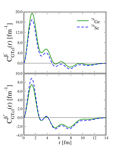
Figure 4: Functions $C(r)$ corresponding to the total strengths $S(\beta^{-})$ and $S(\beta^{+})$ for the initial nucleus ⁷⁶Ge and for the final nucleus ⁷⁶Se.

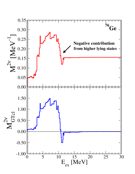
Figure 5: Cumulative contributions to the $M^{2\nu}$ (11) and $M^{2\nu}_{\mathrm{GTcl}}$ (12) as a function of the intermediate state excitation energy. This is for the case of ⁷⁶Ge.

Evaluation of the $2\nu\beta\beta$ closure matrix element

$$M^{2\nu}_{\mathrm{GTcl}}=\langle f|\sum_{k,l}\vec{\sigma}_{k}\cdot\vec{\sigma}_{l}\tau^{+}_{k}\tau^{+}_{l}|i\rangle=\sum_{m}\langle f||\sigma\tau^{+}||m\rangle\langle m||\sigma\tau^{+}||i\rangle~{}$$ (12)

implicitly requires the knowledge of all $1^{+}$ intermediate states and the GT amplitudes connecting them to the initial and final ground states. The expression (12) is a product of amplitudes corresponding to the $\beta^{-}$ strength of the initial nucleus and the $\beta^{+}$ strength of the final one. The total strengths are connected by the Ikeda sum rule $S(\beta^{-})-S(\beta^{+})=3(N-Z)$ which is automatically fulfilled in the QRPA and in the Nuclear Shell Model when the model space involves both spin-orbit partners of all single particle states. In Fig. 4 the radial dependence of these strengths, i.e., the $C(r)$ functions corresponding to $\langle i|\sum_{kl}\tau^{+}_{k}\tau^{-}_{l}\sigma_{k}\cdot\sigma_{l}|i\rangle$, i.e., the $S(\beta^{-})$, and $\langle f|\sum_{kl}\tau^{-}_{k}\tau^{+}_{l}\sigma_{k}\cdot\sigma_{l}|f\rangle$, i.e., the $S(\beta^{+})$, are shown for the case of ⁷⁶Ge and ⁷⁶Se. Note not only the different scales of the two panels, but also the substantial cancellation between the $r\leq 2.5$ fm and $r>2.5$ fm in the $\beta^{+}$ case. The $S(\beta^{+})$ strength is suppressed because the $\beta^{+}$ operator connects states that belong to different isospin multiplets.

While the total strengths represent sums over positive contributions from all $1^{+}$ states in the corresponding odd-odd nuclei, the $M^{2\nu}$ (11) and $M^{2\nu}_{\mathrm{GTcl}}$ (12) matrix elements both depend on the signs of the two amplitudes involved in the product and thus have both positive and negative contributions. In fact, the calculations suggest that, as a function of the $1^{+}$ excitation energy, the contributions are positive at first, but above 5 - 10 MeV negative contributions turn the resulting values of both $M^{2\nu}$ and $M^{2\nu}_{\mathrm{GTcl}}$ sharply down as illustrated in Fig.5. That behavior seems to be again universal. Not only qualitatively similar curve are obtained in QRPA for essentially all $\beta\beta$ decay candidate nuclei, but very similar plot was obtained for ⁴⁸Ca within the nuclear shell model Horoi07 .

In this context it is worthwhile to discuss the so-called single-state dominance (or low-lying states dominance) often invoked in the analysis of the $2\nu\beta\beta$ decay SSD . The ‘staircase’ plot for $M^{2\nu}$ evaluated within QRPA as seen in the upper panel of Fig.5 have the drop at higher energies that is not as steep as in the case of $M^{2\nu}_{\mathrm{GTcl}}$; its magnitude is reduced by the energy denominators.

The contributions to $M^{2\nu}$ are positive at first, followed at energies $\geq$ 5 MeV by several negative ones. Due to this, the true value of $M^{2\nu}$ (0.14 MeV^-1 in the case of ⁷⁶Ge) is reached twice as a function of the excitation energy, once at relatively low $E_{\mathrm{ex}}$ and then again at its asymptotic value. This is a typical situation encountered in most $2\nu\beta\beta$ decay candidate nuclei. In the charge exchange experiments, like e.g. in Ref. Grewe , the GT strength exciting several low-lying $1^{+}$ states is determined in both the $\beta^{-}$ and $\beta^{+}$ directions. Assuming that all contributions to the $M^{2\nu}$ from these states are positive, one usually soon reaches a value that is close to the experimental one. That is considered as indication of the validity of the low-lying states dominance hypothesis. The single (or low-lying) state dominance is also invoked in Refs. coello ; ejiri12 where also a good agreement with the experimental $M^{2\nu}$ matrix element was reached. However, according to our evaluation, some more positive contributions to the $M^{2\nu}$ in such a case are missed, as well as negative contributions from the higher lying $1^{+}$ states. Thus, the low-lying states, while giving by themselves the correct (or almost correct) value of $M^{2\nu}$, miss other contributions which, in particular, are decisively important for the closure matrix element $M^{2\nu}_{\mathrm{GTcl}}$.

It would be clearly desirable to confirm, or reject, the behavior illustrated in Fig. 5. In particular, to check that the $\beta^{+}$ amplitudes above $\sim$ 5 MeV are non-vanishing and that their contribution to $M^{2\nu}$ is indeed negative.

The single state dominance in the $2\nu\beta\beta$ decay can be tested by observing the two- and single-electron spectra SSD1 , in particular at low electron energies. This was done, for example, in the case of ⁸²Se in Ref. SSD3 , indicating its validity. Does it really mean that only low-lying intermediate states contribute to the $M^{2\nu}$ and $M^{2\nu}_{\mathrm{GTcl}}$? As was shown in SSD2 , the deviation of the electron spectrum from the standard form can be described by the Taylor expansion of the energy denominators when the phase space factors are evaluated. The leading correction, called $\xi^{2\nu}_{31}$ there, contains the third power of the energy denominator in the expression analogous to (11). Thus, the quantity $\xi^{2\nu}_{31}$ is dominated by the low lying states and insensitive to the higher lying ones. The indication of single state dominance validity, like those in SSD3 , do not mean that there are no higher lying contributions, and in particular a significant cancellations in the $M^{2\nu}_{\mathrm{GTcl}}$.

The radial dependence $C^{2\nu}_{\mathrm{GTcl}}(r)$ corresponding to the $2\nu\beta\beta$ closure matrix element (12) can be obtained, again, by inserting the Dirac $\delta$-function in between the brackets. Note that while the closure matrix element (12) itself depends only on the $1^{+}$ intermediate states, presence of the $\delta$-function means that all multipoles participate. In Fig.6 we show the resulting radial function for a number of nuclei. The peak at $r\leq$ 2.5 fm is almost fully compensated by the negative tail at larger $r$ values. The actual value of $M^{2\nu}_{\mathrm{GTcl}}$, while always small, depends sensitively on the input parameters (isovector and isoscalar pairing coupling constants).

It is important to add properly the contribution of all $J^{\pi}$ states when evaluating $M^{2\nu}_{\mathrm{GTcl}}$. In Fig.7 we show how the corresponding $C^{2\nu}_{\mathrm{cl}}(r)$ depends on the possible energy cut-off for all $J^{\pi}$ states (lower panel) and the $1^{+}$ states (upper panel). The negative tail becomes deeper, and thus the magnitude of $M^{2\nu}_{\mathrm{GTcl}}$ becomes smaller as more especially $1^{+}$ states are included.

Thus, when the $M^{2\nu}_{\mathrm{GTcl}}$ is evaluated in the shell model using incomplete oscillator shells, with missing spin-orbit partners, as done e.g. in Ref. Xav18 for the $\beta\beta$ candidate nuclei (except ⁴⁸Ca), the results might be uncertain.

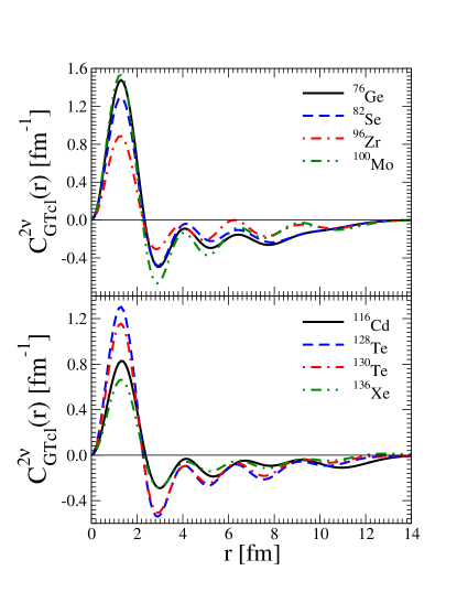
Figure 6: Functions $C^{2\nu}_{\mathrm{GTcl}}(r)$ for several $\beta\beta$ candidate nuclei evaluated within the QRPA.

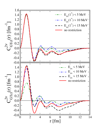
Figure 7: Dependence of the $C^{2\nu}_{\mathrm{GTcl}}(r)$ on the cut-off in the $1^{+}$ excitation energy (upper panel) and all $J^{\pi}$ excitation energies (lower panel) evaluated for the ⁷⁶Ge decay.

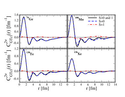
Figure 8: Dependence of the $C^{2\nu}_{\mathrm{GTcl}}(r)$ separated into the spin $S=0$ and $S=1$ components, shown for several $\beta\beta$ decay candidate nuclei.

¿From the way the functions $C^{0\nu}_{\mathrm{GT}}(r)$ and $C^{2\nu}_{\mathrm{GTcl}}(r)$ were constructed, it immediate follows that they are related by

$$C^{0\nu}_{\mathrm{GT}}(r)=H_{\mathrm{GT}}(r,\bar{E})\cdot C^{2\nu}_{\mathrm{GTcl}}(r)~{},$$ (13)

as already pointed out in Ref. SHFV . Therefore, if $C^{2\nu}_{\mathrm{GTcl}}(r)$ were known, the $C^{0\nu}_{\mathrm{GT}}(r)$ can be easily constructed and hence also the $0\nu$ matrix element $M^{0\nu}_{\mathrm{GT}}$. The analogous procedure can be followed, of course, also for $M^{0\nu}_{\mathrm{F}}$ and $M^{0\nu}_{\mathrm{T}}$. But eq. (13) is much more general. Knowing $C^{0\nu}_{\mathrm{GT}}(r)$ or $C^{2\nu}_{\mathrm{GTcl}}(r)$ makes it possible to evaluate the corresponding matrix element for any neutrino potential $H\mathrm{GT}(r,\bar{E})$ like all of those listed in ref. HN17 . That represents, no doubt, a significant practical simplification.

IV Using the $LS$ coupling scheme

¿From the discussion above it is clear that the determination of the correct value of the $2\nu$ closure matrix element $M^{2\nu}_{\mathrm{GTcl}}$ and its radial dependence function $C^{2\nu}_{\mathrm{GTcl}}(r)$ is of primary importance. Insight into this issue can be gained by considering the $LS$ coupling scheme.

Lets divide the $M^{2\nu}_{\mathrm{GTcl}}$ and $M^{2\nu}_{\mathrm{Fcl}}$ into two parts, corresponding to the $S=0$ and $S=1$, where $S$ is the spin of the two decaying neutrons (or spin of the created protons) in their center-of mass system. The corresponding expression is rather complex so we leave it to the Appendix. Having the decomposition of the $M^{2\nu}_{\mathrm{GTcl}}$ and its corresponding radial dependence $C^{2\nu}_{\mathrm{GTcl}}(r)$ into their spin components, we can establish a relation between the GT and F parts.

$$M^{2\nu}_{\mathrm{Fcl}} = (\delta_{S1}+\delta_{S0})\times\langle s1,s2;S\parallel O^{2\nu}_{\mathrm{S}}\parallel s1,s2;S\rangle,$$

$$M^{2\nu}_{\mathrm{GTcl}} = (\delta_{S1}-3\delta_{S0})\times\langle s1,s2;S\parallel O^{2\nu}_{\mathrm{S}}\parallel s1,s2;S\rangle.$$

Therefore, for the closure matrix elements

$$M^{2\nu}_{\mathrm{GT},S=0} = -3\times M^{2\nu}_{\mathrm{F},S=0}$$ (15)

$$M^{2\nu}_{\mathrm{GT},S=1} = M^{2\nu}_{\mathrm{F},S=1}.$$ (16)

These are exact relations. The radial functions $C^{2\nu}_{\mathrm{Fcl,GTcl}}(r)(S)$ obey them as well.

Example of this separation are shown in Fig. 8. Clearly, the $S=0$ component accounts for essentially the whole $C^{2\nu}_{\mathrm{GTcl}}(r)$ function; the $S=1$ component is negligible. Note that the standard like nucleon pairing supports the dominance of the $S=0$ component.

Isospin is a good quantum number in nuclei, $T=(N-Z)/2$ in the ground states; the admixtures of higher values of $T$ is negligible for our purposes. From this it immediately follows that $M^{2\nu}_{\mathrm{Fcl}}=0$. That relation is obeyed automatically in the nuclear shell model where isospin is a good quantum number by construction. In QRPA, however, the isospin is, generally, not conserved. It was shown in isospin that partial restoration of the isospin symmetry, and validity of the $M^{2\nu}_{\mathrm{Fcl}}=0$, can be achieved within the QRPA by choosing the isospin symmetry for the $T=1$ nucleon-nucleon interaction, i.e., by choosing the same strength for the neutron-neutron and proton-proton pairing force treated within the BCS method, and the isovector neutron-proton interaction treated by the QRPA equations of motion. (In practice, the five effective coupling constants are close to each other, but not exactly equal since the renormalization of the pairing strength couplings $d_{nn}^{i,f}$ and $d_{pp}^{i.f}$ are adjusted to reproduce the corresponding neutron and proton gaps and the neutron-proton isovector coupling renormalization $g_{pp}^{T=1}$ is chosen to reproduce the $M^{2\nu}_{\mathrm{Fcl}}=0$ relation.) The values of these parameters are shown in Table 1.

$M^{2\nu}_{\mathrm{Fcl}}=0$ follows from the isospin conservation and implies that $M_{S=0}=-M_{S=1}$. However, both could be large in absolute value. In Fig 8 QRPA results for $M_{\mathrm{Fcl}}$=0 and $M_{\mathrm{GTcl}}$=0 are presented. In that case there is a significant difference in behavior of $C(r)$ for the $S=0$ and $S=1$, with the $S=0$ part significantly larger that the $S=1$ part. Note that in QRPA the values of $M_{\mathrm{Fcl}}$=0 and $M_{\mathrm{GTcl}}$=0 depend on the already fixed renormalization strength $g_{pp}^{T=1}$ and on the value of $g_{pp}^{T=0}$. The $M_{S=0}$ values in Fig 8 are in agreement with the discussion in the preceding section, where we saw that their values are numerically close to zero, actually oscillating between the positive and negative values for different nuclei, and depending sensitively on the properties of the poorly known higher lying $1^{+}$ states.

We can fulfil the relation $M^{2\nu}_{\mathrm{GTcl}}=0$ by adjustment of the renormalization of the isoscalar neutron-proton coupling strength $g^{T=0}_{pp}$. As we effectively restored the isospin symmetry by the proper choice of $g^{T=1}_{pp}$, choosing $g^{T=0}_{pp}$ so that $M^{2\nu}_{\mathrm{GTcl}}=0$, corresponds to the partial restoration of the spin-isospin symmetry $\mathrm{SU}(4)$. Obviously, choosing the effective neutron-proton interaction in this way is quite different from the proposal in ref. Xav18 where the proportionality between $M^{0\nu}_{\mathrm{GT}}$ and $M^{2\nu}_{\mathrm{GTcl}}$ was proposed. We believe that assuming that $M^{2\nu}_{\mathrm{GTcl}}\sim 0$ reflects better the physics of the problem. Once the $M^{2\nu}_{\mathrm{GTcl}}$ and $M^{2\nu}_{\mathrm{Fcl}}$ have been fixed, the corresponding radial functions $C^{2\nu}_{\mathrm{GTcl}}(r)$ can be obtained, and from them, using Eq. (13), the values of $M^{0\nu}_{\mathrm{F}}$ and $M^{0\nu}_{\mathrm{GT}}$ can be obtained. The results are described and discussed in the following section.

Since we know the experimental values of the $2\nu\beta\beta$ matrix elements $M^{2\nu}$, it is legitimate to ask whether the fact that they do not vanish can be compatible with our assumption that the closure matrix elements $M^{2\nu}_{\mathrm{GTcl}}$ vanish. Clearly, if $\bar{E}_{av}$ is the properly averaged energy denominator, then

$$\bar{E}\times M^{2\nu}=M^{2\nu}_{\mathrm{GTcl}}$$ (17)

must be obeyed. If the right-hand side of this equation is vanishing, then one of the factors on the left-hand side must vanish as well. In our case it must be the average energy $\bar{E}$ reflecting the fact that in both $M^{2\nu}$ and $M^{2\nu}_{\mathrm{GTcl}}$ are both positive and negative contributions to the corresponding sums (by treating the negative sign in the numerator of (11) as negative denominator).

In our approach the parameter $g^{T=0}_{pp}$ is fixed by the requirement that $M^{2\nu}_{\mathrm{GTcl}}=0$, it is thus straightforward to evaluate, within QRPA, the $M^{2\nu}$ and compare them with their experimental values derived from the observed $2\nu\beta\beta$ half-lives. In agreement with the idea of ‘$g_{\rm A}$ quenching’, the calculated matrix elements are typically larger than the experimental values. That discrepancy can be, at least in part, remedied by choosing the effective $g_{\rm A}$ value, $g_{\rm A}^{\mathrm{eff}}=q\times g_{\rm A}^{\mathrm{free}}$. (Even somewhat better agreement is achieved by assuming that $g_{\rm A}^{\mathrm{eff}}$ scales like $1/A^{1/2}$. We do not see any obvious justification for such a dependence, and use $g_{\rm A}^{\mathrm{eff}}$ independent of A.) Taking the average ratio of the calculated and experimental matrix elements, we arrive at $q=0.712$. The resulting quenched calculated matrix elements are compared with the experimental ones in Table 1. The agreement is only within a factor of $\sim 2$, reflecting the known strong sensitivity of $M^{2\nu}$ on the $g^{T=0}_{pp}$ values.

Table 1: Renormalization parameters of the pairing interaction $d^{i,f}_{p,n}$ (i- initial nucleus, f-final nucleus, p-protons, n-neutrons) adjusted to reproduce experimental pairing gaps. Renormalization parameters of the isovector $g^{T=1}_{pp}$ and isoscalar $g^{T=0}_{pp}$ particle-particle interactions of the residual Hamiltonian adjusted to reproduce, respectively, $M^{2\nu}_{\mathrm{Fcl}}=0$ and $M^{2\nu}_{\mathrm{GTcl}}=0$ - an effective restoration of the isospin $\mathrm{SU}(2)$ and spin-isospin $\mathrm{SU}(4)$. The corresponding values of the $2\nu\beta\beta$-decay Fermi $M^{2\nu}_{\mathrm{F}}$ and Gamow-Teller $M^{2\nu}_{\mathrm{GT}}\times q^{2}$ matrix elements, where $q=0.712$ is the effective quenching factor, $g_{\rm A}^{\rm eff}=q\times g_{\rm A}^{\rm free}=0.904$. In the last column are the experimentally determined matrix elements $M^{2\nu}_{\mathrm{exp}}$ for unquenched $g_{\rm A}$.

Nucleus		$d^{i}_{pp}$	$d^{f}_{pp}$		$d^{i}_{nn}$	$d^{f}_{nn}$		$g^{T=1}_{pp}$	$g^{T=0}_{pp}$		$M^{2\nu}_{F}$	$M^{2\nu}_{\mathrm{GT}}\times q^{2}$	$M^{2\nu}_{\mathrm{exp}}$
											[MeV-1]	[MeV-1]	[MeV-1]
48Ca		-	1.069		-	0.982		1.028	0.745		-0.003	0.019	0.046
76Ge		0.922	0.960		1.053	1.085		1.021	0.733		0.003	0.077	0.136
82Se		0.861	0.921		1.063	1.108		1.016	0.737		0.001	0.071	0.100
96Zr		0.910	0.984		0.752	0.938		0.961	0.739		0.001	0.162	0.097
100Mo		1.000	1.021		0.926	0.953		0.985	0.799		-0.001	0.306	0.251
116Cd		0.998	-		0.934	0.890		0.892	0.877		-0.000	0.059	0.136
128Te		0.816	0.857		0.889	0.918		0.965	0.741		0.017	0.076	0.052
130Te		0.847	0.922		0.971	1.011		0.963	0.737		0.016	0.065	0.037
136Xe		0.782	0.885		-	0.926		0.910	0.685		0.014	0.036	0.022

V $0\nu\beta\beta$ matrix elements and the partial $\mathrm{SU}(4)$ symmetry restoration.

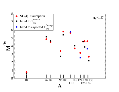
Figure 9: $M^{0\nu}$ evaluated when $g_{pp}^{T=0}$ is adjusted so that the $2\nu$ half-life is correctly reproduced (black squares) or by requiring that $M^{2\nu}_{\mathrm{GTcl}}=0$, i.e., partial restoration of the $\mathrm{SU}(4)$ symmetry.

The matrix elements $M^{2\nu}$ of the $2\nu\beta\beta$ decay involve only $1^{+}$ virtual intermediate states. Within the QRPA they sensitively depend on the magnitude of the isoscalar neutron-proton interaction martin , conventionally denoted as $g_{pp}^{T=0}$. On the other hand, matrix elements $M^{0\nu}$ of the $0\nu\beta\beta$ decay contain many multipoles of the intermediate states. Among them the $1^{+}$, or GT, is particularly sensitive to the $g_{pp}^{T=0}$; other multipoles are less dependent to its magnitude. That led to the practice us1 ; us2 , commonly used in QRPA now, to adjust the $g_{pp}^{T=0}$ so that the experimental half-life $T^{2\nu}_{1/2}$ is correctly reproduced. That way the most sensitive multipole contributing to $M^{0\nu}$ has been tied to the experimentally determined quantity. (Also, it turns out that with this adjustment, the magnitude of $M^{0\nu}$ becomes essentially independent on the size of the single particle basis included.)

As explained above, in this work we propose instead to use the condition $M^{2\nu}_{\mathrm{GTcl}}=0$, i.e., partial restoration of the $\mathrm{SU}(4)$ symmetry, to adjust the value of the renormalization parameter $g_{pp}^{T=0}$. The matrix elements $M^{0\nu}$ evaluated by these two alternative methods are shown in Table 2 together with the corresponding partial values $M_{\mathrm{F}}$, $M_{\mathrm{GT}}$ and $M_{\mathrm{T}}$ separated into the spin $S=0$ and $S=1$ components. Few candidate nuclei (⁹⁴Zr, ¹¹⁰Pd, ¹²⁴Sn and ¹³⁴Xe), where the $2\nu$ decay has not been observed as yet, are also included in Table 2. All entries there were obtained when the sum over the virtual intermediate states was explicitly evaluated. When the closure approximation is used together with the $\mathrm{SU}(4)$ adjustment, the results are similar, with the final $M^{0\nu}$ values about 10% smaller, similar to the previous experience described above. Typically, the contributions of the spin $S=1$ component to the $M_{\mathrm{F}}$ and $M_{\mathrm{GT}}$ are indeed negligible. However, the tensor mart, $M_{\rm T}$ gets its value only from $S=1$; it constitutes about 10% of the total $M^{0\nu}$ value.

Adjusting $g_{pp}^{T=0}$ to the condition of partial restoration of the $\mathrm{SU}(4)$ symmetry means that the $2\nu$ matrix elements (and, naturally, the half-lives $T^{2\nu}_{1/2}$) are not any longer tied to their experimental values. The theoretical values of $M^{2\nu}$ are only in qualitative agreement with experiment, as we saw in the previous section. However, remarkably, the new adjustment of $g_{pp}^{T=0}$ causes only relatively small changes in the $M^{0\nu}$ as one could see in Table 2. In Fig. 9 the two ways of the $g_{pp}^{T=0}$ adjustment are compared. The largest effect, for ¹³⁰Te and ¹³⁶Xe is an increase of $M^{0\nu}$ by $\sim$ 20%. Note that both variants shown in Fig. 9 were evaluated with $g_{\rm A}=1.27$, i.e., without quenching.

Table 2: The nuclear matrix elements (NME) associated with light neutrino mass mechanism of the $0\nu\beta\beta$-decay calculated within the proton-neutron QRPA using two ways of fixing the strengths of residual interactions in the nuclear Hamiltonian: i) $g^{T=1}_{pp}$ and $g^{T=0}_{pp}$ are adjusted to reproduce $M^{2\nu}_{\mathrm{F}}=0$ and the experimental $2\nu\beta\beta$ half-life, respectively ($T^{2\nu}_{1/2}$); ii) $g^{T=1}_{pp}$ and $g^{T=0}_{pp}$ are adjusted to reproduce $M^{2\nu}_{\mathrm{Fcl}}=0$ and $M^{2\nu}_{\mathrm{GTcl}}=0$ - an effective restoration of the isospin $\mathrm{SU}(2)$ and spin-isospin $\mathrm{SU}(4)$ symmetry. In i) and ii) the sum over all virtual excitations is explicitly performed. The partial Fermi, Gamow-Teller, tensor and full $0\nu\beta\beta$-decay NME are presented for $S=0$ and $S=1$ channels and for the sum of them. Unquenched value of axial-vector coupling constant ($g_{\rm A}=1.269$), Argonne two-nucleon short-range correlations and $\bar{E}=8$ MeV are considered.

Nucl.	par.		S=0					S=1					full NME
			$M_{\rm F}$	$M_{\mathrm{GT}}$	$M_{\rm T}$	$M^{0\nu}$		$M_{\rm F}$	$M_{\mathrm{GT}}$	$M_{\rm T}$	$M^{0\nu}$		$M_{\rm F}$	$M_{\mathrm{GT}}$	$M_{\rm T}$	$M^{0\nu}$
48Ca	$T^{2\nu}_{1/2}$		-0.253	0.659	0.00	0.816		-0.027	-0.021	-0.156	-0.161		-0.280	0.638	-0.156	0.656
	$\mathrm{SU}(4)$		-0.285	0.748	0.00	0.925		0.006	0.009	-0.158	-0.153		-0.280	0.757	-0.158	0.773
76Ge	$T^{2\nu}_{1/2}$		-1.719	4.482	0.00	5.550		0.111	0.102	-0.588	-0.554		-1.608	4.584	-0.588	4.995
	$\mathrm{SU}(4)$		-1.705	4.443	0.00	5.502		0.097	0.089	-0.588	-0.559		-1.570	4.455	-0.583	4.846
82Se	$T^{2\nu}_{1/2}$		-1.537	3.995	0.00	4.949		0.037	0.035	-0.544	-0.532		-1.500	4.029	-0.544	4.417
	$\mathrm{SU}(4)$		-1.587	4.133	0.00	5.119		0.089	0.082	-0.540	-0.513		-1.499	4.216	-0.540	4.606
94Zr	$\mathrm{SU}(4)$		-1.171	3.066	0.00	3.793		-0.066	-0.050	-0.392	-0.401		-1.237	3.016	-0.392	3.392
96Zr	$T^{2\nu}_{1/2}$		-0.916	2.359	0.00	2.928		-0.272	-0.242	-0.420	-0.494		-1.188	2.117	-0.420	2.435
	$\mathrm{SU}(4)$		-1.174	3.069	0.00	3.798		-0.008	-0.001	-0.405	-0.401		-1.182	3.068	-0.405	3.396
100Mo	$T^{2\nu}_{1/2}$		-1,799	4.658	0.00	5.775		-0.410	-0.362	-0.707	-0.814		-2.209	4.296	-0.707	4.961
	$\mathrm{SU}(4)$		-2.038	5.327	0.00	6.592		-0.168	-0.136	-0.692	-0.724		-2.206	5.191	-0.692	5.868
110Pd	$\mathrm{SU}(4)$		-1.961	5.115	0.00	6.332		-0.174	-0.145	-0.607	-0.643		-2.135	4.970	-0.607	5.689
116Cd	$T^{2\nu}_{1/2}$		-1.280	3.328	0.00	4.123		0.274	-0.235	-0.290	-0.355		-1.554	3.093	-0.290	3.768
	$\mathrm{SU}(4)$		-1.272	3.305	0.00	4.095		-0.283	-0.243	-0.291	-0.358		-1.555	3.062	-0.291	3.737
124Sn	$\mathrm{SU}(4)$		-1.096	2.862	0.00	3.543		0.032	0.031	-0.347	-0.336		-1.064	2.894	-0.347	3.207
128Te	$T^{2\nu}_{1/2}$		-1.638	4.248	0.00	5.265		-0.146	-0.125	-0.604	-0.638		-1.784	4.122	-0.604	4.626
	$\mathrm{SU}(4)$		-1.839	4.784	0.00	5.923		-0.044	-0.033	-0.588	-0.594		-1.878	4.751	-0.588	5.329
130Te	$T^{2\nu}_{1/2}$		-1.411	3.655	0.00	4.531		-0.162	-0.140	-0.554	-0.593		-1.573	3.515	-0.554	3.939
	$\mathrm{SU}(4)$		-1.616	4.215	0.00	5.219		-0.053	-0.042	-0.536	-0.545		-1.669	4.173	-0.536	4.673
134Xe	$\mathrm{SU}(4)$		-1.598	4.163	0.00	5.156		-0.044	-0.034	-0.498	-0.504		-1.642	4.129	-0.498	4.652
136Xe	$T^{2\nu}_{1/2}$		-0.780	2.009	0.00	2.493		-0.035	-0.028	-0.285	-0.291		-0.815	1.980	-0.285	2.202
	$\mathrm{SU}(4)$		-0.927	2.410	0.00	2.985		0.022	0.022	-0.274	-0.266		-0.905	2.432	-0.274	2.720

VI Summary

In this work we discuss the importance of dependence of the $0\nu$ and $2\nu$ nuclear matrix elements on the distance $r_{ij}$ between the two neutrons that are transformed in two protons in the double-beta decay. We show that, if this function, $C(r)$, is known for any particular mechanism of the decay, evaluation of the matrix element for any other mechanism is reduced to an integral using Eq. (13).

Further, we show that there is a close relation between the GT part of the $M^{0\nu}$ and the matrix element of the experimentally observed $2\nu\beta\beta$ decay, evaluated however in the closure approximation, $M^{2\nu}_{\mathrm{cl}}$. Our work does not support the conjecture in Ref.Xav18 of proportionality between the $M^{0\nu}_{\mathrm{GT}}$ and $M^{2\nu}_{\mathrm{cl}}$. Instead, we argue that the positive contributions to $M^{2\nu}_{\mathrm{cl}}$ from the lower lying $1^{+}$ intermediate states is essentially fully cancelled by the negative contribution of the higher lying $1^{+}$ states. We also show that the contribution of the triplet spin $S=1$ two neutron states is much smaller than the contribution of the singlet $S=0$ states. (Note that when $M^{2\nu}_{\rm F}$ = 0 the $S=0$ part is always three times larger that the $S=1$ part.) From these considerations follows a simple proportionality between the Fermi and GT parts of the $M^{2\nu}_{\mathrm{cl}}$.

Based on these consideration we arrive at a new way of adjusting the important QRPA parameter, the renormalization of the isoscalar particle-particle interaction, $g_{pp}^{T=0}$. We propose that its value should be determined from the requirement that $M^{2\nu}_{\mathrm{GTcl}}=0$. Together with $M^{2\nu}_{\mathrm{Fcl}}=0$, following from isospin conservation, these two condition are equivalent to the restoration of partial conservation of spin-isospin $\mathrm{SU}(4)$ symmetry.

We then evaluate the true $2\nu$ matrix elements and compare them to the corresponding experimental values. The calculated $M^{2\nu}$ values are mostly larger than the experimental ones, suggesting on average a relatively modest quenching $g_{\rm A}^{\mathrm{eff}}=0.710\times g_{\rm A}^{\mathrm{free}}$. The agreement between the calculated and experimental values of $M^{2\nu}$ is, however, only qualitative. That is, perhaps, not surprising given the strong dependence of the calculated $M^{2\nu}$ values on the $g_{pp}^{T=0}$.

The $0\nu$ matrix elements, corresponding to the “standard” light Majorana neutrino exchange are evaluated next using the new adjustment of the $g_{pp}^{T=0}$. When they are compared to the values obtained when $g_{pp}^{T=0}$ is chosen so that the $2\nu$ half-life is correctly reproduced, which was a QRPA standard procedure until now, only relatively modest changes of the $M^{0\nu}$ are obtained. This shows that, within QRPA, the $M^{0\nu}$ values are quite stable. It also, in our opinion, represents a better way to determine the parameter $g_{pp}^{T=0}$, and through the corresponding function $C^{2\nu}_{\mathrm{GTcl}}(r)$ all possible $0\nu$ nuclear matrix elements.

VII Acknowledgment

This work was supported by the VEGA Grant Agency of the Slovak Republic under Contract No. 1/0922/16, by Slovak Research and Development Agency under Contract No. APVV-14-0524, RFBR Grant No. 16-02-01104, Underground laboratory LSM - Czech participation to European-level research infrastructure CZ.02.1.01/0.0/0.0/16 013/0001733. The work of P.V. is supported by the Physics Department, California Institute of Technology.

VIII Appendix: $LS$ coupling scheme

In the QRPA the closure matrix element ${M}^{\alpha}_{K}$ ($\alpha=0\nu,~{}2\nu$ and $K=\mathrm{F}$ (Fermi), $\mathrm{GT}$ (Gamow-Teller) and $\mathrm{T}$ (Tensor)) can be written as a sum over two neutron (initial nucleus) and two proton (final nucleus) states participating in the two virtual beta decays inside nucleus, angular momentum $\mathcal{J}$ to which they are coupled, and angular momentum and parity $J^{\pi}$ of the intermediate nucleus as follows:

$$M^{\alpha}_{K} = \sum_{pnp^{\prime}n^{\prime}}\sum_{J^{\pi}\mathcal{J}}(-1)^{j_{n}+j_{p^{\prime}}+J+{\mathcal{J}}}\sqrt{2{\mathcal{J}}+1}\times\qquad\qquad$$ (21)

$$\left\{\begin{array}[]{c c c}j_{p}&j_{n}&J\\ j_{n^{\prime}}&j_{p^{\prime}}&{\mathcal{J}}\end{array}\right\}~{}D(p^{\prime}n^{\prime},pn;J^{\pi})~{}T^{\alpha}_{K}(pp^{\prime},nn^{\prime};{\mathcal{J}}),$$

where

$$D(p^{\prime}n^{\prime},pn,J^{\pi}) = \sum_{J^{\pi},k_{i},k_{f}}\langle 0_{f}^{+}\parallel[\widetilde{c_{p^{\prime}}^{+}\tilde{c}_{n^{\prime}}}]_{J}\parallel J^{\pi}k_{f}\rangle\times$$

$$\langle J^{\pi}k_{f}|J^{\pi}k_{i}\rangle\langle J^{\pi}k_{i}\parallel[c_{p}^{+}\tilde{c}_{n}]_{J}\parallel 0_{i}^{+}\rangle\,$$

includes products of reduced matrix elements of one-body densities $c_{p}^{+}\tilde{c}_{n}$ ($\tilde{c}_{n}$ denotes the time-reversed state) connecting the initial nuclear ground state with the final nuclear ground state through a complete set of states of the intermediate nucleus labeled by their angular momentum and parity, $J^{\pi}$, and indices $k_{i}$ and $k_{f}$. They depend on the BCS coefficients $u_{i},v_{j}$ and on the QRPA vectors $X,Y$ isospin . The coupling $(lsj)$ for each single proton (neutron) state is considered, i.e., the individual orbital momentum $l_{p}$ ($l_{n}$) and spin $s_{p}$ ($s_{n}$) is coupled to the total angular momentum $j_{p}$ ($j_{n}$). The non-antisymmetrized two-nucleon matrix element takes the form

$$T^{\alpha}_{K}(pp^{\prime},nn^{\prime};{\mathcal{J}})=\langle p(1)p^{\prime}(2);{\mathcal{J}}\parallel{\cal O}^{\alpha}_{K}\parallel n(1)n^{\prime}(2);{\mathcal{J}}\rangle$$

where

$${\cal O}^{2\nu}_{\rm F}=1,~{}~{}~{}~{}{\cal O}^{2\nu}_{\mathrm{GT}}=\sigma_{12},~{}~{}~{}~{}{\cal O}^{2\nu}_{\rm T}=S_{12}$$

$${\cal O}^{0\nu}_{\mathrm{F,GT,T}}(r_{12})={\cal O}^{2\nu}_{\mathrm{F,GT,T}}~{}H_{K}(r_{12},\bar{E})$$ (24)

with $S_{12}=3(\vec{\sigma}_{1}\cdot\hat{r}_{12})(\vec{\sigma}_{2}\cdot\hat{r}_{12})-\sigma_{12}$, $\sigma_{12}=\vec{\sigma}_{1}\cdot\vec{\sigma}_{2}$. $\vec{r}_{12}=\vec{r}_{1}-\vec{r}_{2}$, ${r}_{12}=|\vec{r}_{12}|$ and $\hat{r}_{12}=\vec{r}_{12}/r_{12}$, where $\vec{r}_{1}$ and $\vec{r}_{2}$ are coordinates of nucleons undergoing beta decay. For the exchange of light Majorana neutrinos, the $0\nu\beta\beta$ decay mechanism we are considering here, the neutrino potentials $H_{K}(r_{12},\bar{E})$ are given in Eq. (II)

It practice, the calculation of non-antisymmetrized two-nucleon matrix element in Eq. (VIII) is performed in center of mass frame by using a harmonic oscillator single particle basis set. The transformation from $jj$ to $LS$ coupling is used and the Talmi transformation via the Moshinsky transformation brackets is considered. In the case of the $0\nu\beta\beta$-decay two-nucleon matrix elements we obtain

$$\left(\begin{array}[]{l}T^{0\nu}_{\rm F}\\ T^{0\nu}_{\mathrm{GT}}\\ T^{0\nu}_{\rm T}\end{array}\right)(pp^{\prime},nn^{\prime};{\mathcal{J}})=\hat{\mathcal{J}}\hat{j}_{n}\hat{j}_{n^{\prime}}\hat{j}_{p}\hat{j}_{p^{\prime}}\sum\limits_{SL}(2S+1)\times$$ (28)

$$~{}~{}~{}~{}~{}(2L+1)\left\{\begin{array}[]{lll}1/2&l_{p}&j_{p}\\ 1/2&l_{p^{\prime}}&j_{p^{\prime}}\\ S&L&{\mathcal{J}}\end{array}\right\}\left\{\begin{array}[]{lll}1/2&l_{n}&j_{n}\\ 1/2&l_{n^{\prime}}&j_{n^{\prime}}\\ S&L&{\mathcal{J}}\end{array}\right\}\times$$ (35)

$$\sum\limits_{nln^{\prime}l^{\prime}\atop{\cal NL}}\langle nl,{\cal NL},L|n_{p}l_{p},n_{p^{\prime}}l_{p^{\prime}},L\rangle\times$$

$$~{}~{}~{}~{}~{}~{}~{}\langle n^{\prime}l^{\prime},{\cal NL},L|n_{n}l_{n},n_{n^{\prime}}l_{n^{\prime}},L\rangle\sum\limits_{J^{\prime}}(2J^{\prime}+1)\times$$

$$~{}~{}~{}~{}~{}~{}\sqrt{(2l+1)(2l^{\prime}+1)}\left\{\begin{array}[]{l@{\,}l@{\,}l}l&L&{\cal L}\\ {\cal J}&J^{\prime}&S\end{array}\right\}\left\{\begin{array}[]{l@{\,}l@{\,}l}l^{\prime}&L&{\cal L}\\ {\cal J}&J^{\prime}&S\end{array}\right\}\times$$ (40)

$$~{}~{}\langle nl,S;J^{\prime}|\left(\begin{array}[]{c}(~{}~{}\delta_{S0}+\delta_{S1})H_{\rm F}(r_{12},\bar{E})\\ (-3\delta_{S0}+\delta_{S1})H_{\mathrm{GT}}(r_{12},\bar{E})\\ S_{12}H_{\rm T}(r_{12}.\bar{E})\end{array}\right)|n^{\prime}l^{\prime},S;J^{\prime}\rangle.$$ (44)

Here, $\hat{\cal J}=\sqrt{2{\cal J}+1}$ and $\hat{j}_{\alpha}=\sqrt{2j_{\alpha}+1}$ with $\alpha=p,~{}p^{\prime},~{}n$ and $n^{\prime}$ . We note that in the case of the Fermi and Gamow-Teller transitions there are both $S=0$ an $S=1$ contributions, unlike the case of the tensor transition where only $S=1$ is allowed. Due to the presence of neutrino potentials $H_{K}(r_{12},\bar{E})$ ($K=\mathrm{F}$, $\mathrm{GT}$ and $\mathrm{T}$) in two-body transition operators there is dominance of the $S=0$ contribution to $M^{0\nu}$. There is a small difference between the Fermi and Gamow-Teller neutrino potentials due to a different form factor’s cut-off and contributions from higher order terms of the nucleon currents. If they would be equal, and the $S=1$ contribution could be neglected, we would end up with

$$M^{0\nu}_{\mathrm{GT}}\simeq-3M^{0\nu}_{\mathrm{F}}.$$ (46)

The $2\nu\beta\beta$-decay Fermi and Gamow-Teller matrix elements can be decomposed into the $S=0$ and $S=1$ contributions as follows (see Eq. (LABEL:eq:sepr)):

$$M^{2\nu}_{\mathrm{GT}} = -3M^{2\nu}_{S=0}+M^{2\nu}_{S=1},$$

$$M^{2\nu}_{\mathrm{F}} = ~{}~{}~{}~{}M^{2\nu}_{S=0}+M^{2\nu}_{S=1}$$ (47)

The corresponding decomposition of the non-antisymmetrized two-nucleon matrix element is given by

$$\left(\begin{array}[]{l}T^{2\nu}_{\rm F}\\ T^{2\nu}_{\mathrm{GT}}\end{array}\right)(pp^{\prime},nn^{\prime};{\mathcal{J}})=\hat{\mathcal{J}}\hat{j}_{n}\hat{j}_{n^{\prime}}\hat{j}_{p}\hat{j}_{p^{\prime}}\sum\limits_{SL}(2S+1)\times$$ (50)

$$~{}~{}~{}~{}~{}(2L+1)\left\{\begin{array}[]{lll}1/2&l_{p}&j_{p}\\ 1/2&l_{p^{\prime}}&j_{p^{\prime}}\\ S&L&{\mathcal{J}}\end{array}\right\}\left\{\begin{array}[]{lll}1/2&l_{n}&j_{n}\\ 1/2&l_{n^{\prime}}&j_{n^{\prime}}\\ S&L&{\mathcal{J}}\end{array}\right\}\times$$ (57)

$$~{}~{}~{}~{}~{}\delta_{n_{p}n_{p^{\prime}}}\delta_{l_{p}l_{p^{\prime}}}\delta_{n_{n}n_{n^{\prime}}}\delta_{l_{n}l_{n^{\prime}}}\times\left(\begin{array}[]{c}\delta_{S0}+\delta_{S1}\\ -3\delta_{S0}+\delta_{S1}\\ \end{array}\right)$$ (60)

If $M^{2\nu}_{\mathrm{F}}=0$ because of isospin conservation (see isospin ), then $S=0$ and $S=1$ contributions are equal in magnitude but opposite in sign.

References

- (1) J. Schechter and J.W.F. Valle, Phys.Rev.D 25, 2951 (1982).
- (2) J. Engel and J. Menendez, Rept. Prog. Phys. 80, 046301 (2017).
- (3) F. Šimkovic, R. Hodák, A. Faessler, and P. Vogel, Phys. Rev. C 83, 015502 (2011).
- (4) C. Patrignani et al. [Particle Data Group], Chin. Phys. C 40, 100001 (2016) and update 2017.
- (5) F. Šimkovic, A. Faessler, V. A. Rodin, P. Vogel, and J. Engel, Phys. Rev. C 77, 045503 (2008).
- (6) F. Šimkovic, G. Pantis, J. D. Vergados, and A. Faessler, Phys. Rev. C 60, 055502 (1999).
- (7) F. Šimkovic, A. Faessler, H. Muther, V. Rodin, and M. Stauf, Phys. Rev. C 79, 055501 (2009).
- (8) J. Kotila and F. Iachello, Phys. Rev. C 85, 034316 (2012).
- (9) M. Horoi and A. Neacsu, arXiv:1706.05391[hep-ph].
- (10) R. A. Sen’kov and M. Horoi, Phys. Rev. C 90, 051301 (2014).
- (11) J. Menendez et al. Nucl. Phys. A 818, 130 (2009).
- (12) S. Pastore et al., Phys. Rev. C 97, 014606 (2018).
- (13) M. Horoi, S. Stoica and B.A. Brown, Phys.Rev.C 75, 034303 (2007).
- (14) J. Abad, A. Morales, R. Nunez-Lagos, and A.F. Pacheco, An. Fis. A 80, 9 (1984); J. Phys. (Paris) 45, 147 (1984).
- (15) E.W. Grewe et al., Phys. Rev. C 78, 044301 (2008).
- (16) E.A. Coello-Perez, J. Menendez and A. Schwenk, arXiv:1708.06140[nucl-th].
- (17) H. Ejiri, J. Phys. Soc. Japan 81, 033201 (2012).
- (18) P. Domin, S. Kovalenko, F. Šimkovic and S.V. Semenov, Nucl. Phys. A753, 337 (2005).
- (19) R. Arnold et al., arXiv:1806.05553[hep-ex].
- (20) F. Šimkovic, R. Dvornický, D. Štefánik and A. Faessler, Phys. Rev. C 97, 034315 (2018).
- (21) N. Shimizu, J. Menendez and K. Yako, Phys.Rev.Lett.120, 142502 (2018).
- (22) F. Šimkovic, V. A. Rodin, A. Faessler, and P. Vogel, Phys. Rev. C 87, 045501(2013).
- (23) P. Vogel and M.R. Zirnbauer, Phys. Rev. Lett.57, 3148 (1986).
- (24) V. A. Rodin, A. Faessler, F. Šimkovic and P. Vogel, Phys. Rev. C 68, 044302(2003).
- (25) V. A. Rodin, A. Faessler, F. Šimkovic and P. Vogel, Nucl. Phys. A766, 107 (2006), and erratum A793, 213 (2007).