Density-driven correlations in many-electron ensembles:
theory and application for excited states

Abstract

Density functional theory can be extended to excited states by means of a unified variational approach for passive state ensembles. This extension overcomes the restriction of the typical density functional approach to ground states, and offers useful formal and demonstrated practical benefits. The correlation energy functional in the generalized case acquires higher complexity than its ground state counterpart, however. Little is known about its internal structure nor how to effectively approximate it in general. Here we show that such a functional can be broken down into natural components, including what we call “state-” and “density-driven” correlations, with the former amenable to conventional approximations, and the latter being a unique feature of ensembles. Such a decomposition, summarised in eq. (6), provides us with a pathway to general approximations that are able to routinely handle low-lying excited states. The importance of density-driven correlations is demonstrated, an approximation for them is introduced and shown to be useful.

Electronic structure theory has transformed the study of chemistry, materials science and condensed matter physics, by enabling quantitative predictions using computers. But a general solution to the many-electron problem remains elusive, because the electron-electron interactions imply highly non-trivial correlations among the relevant degrees of freedoms. Out of the numerous electronic structure methodologies, density functional theory Hohenberg and Kohn (1964); Kohn and Sham (1965); Jones (2015) (DFT) has become the dominant approach thanks to its balance between accuracy and speed, achieved by using the electron density as the basic variable, then mapping the original interacting problem onto an auxiliary non-interacting problem.

DFT gives access to ground states, but not excited states, meaning alternatives must be used for important processes like photochemistry or exciton physics Matsika and Krylov (2018). Its time-dependent extension (TDDFT) does offer access to excited states at reasonable cost Runge and Gross (1984); Casida and Huix-Rotllant (2012), and is thus commonly employed for this purpose. Routine applications of TDDFT reuse ground-state approximations by evaluating them on the instantaneous density, the so-called adiabatic approximation. This approach fails badly, however, when many-body correlations defy a time-dependent mean-field picture, including for important charge transfer excitations Ullrich and Tokatly (2006); Maitra (2017).

One highly promising alternative involves tackling both ground and excited eigenstates by means of one and the same density functional approach Theophilou (1979); Gross et al. (1988a, b); Oliveira et al. (1988), using ensemble DFT (EDFT). EDFT is appealing because it can automatically deal with otherwise difficult orthogonality conditions and can potentially tap into more than 30 years of density functional approximation development. EDFT has been shown to solve problems that are difficult for TDDFT, such as charge transfers, double excitations, and conical intersections Filatov and Shaik (1999); Filatov et al. (2015); Filatov (2015, 2016); Franck and Fromager (2014); Deur et al. (2017); Pribram-Jones et al. (2014a); Yang et al. (2014, 2017); Gould et al. (2018); Sagredo and Burke (201).

Consolidating the preliminary success of EDFT into useful approximations requires further understanding of how many-body correlations get encoded in EDFT and how they can be approximated generally. The correlation energy of many-electron ground states is traditionally divided into dynamical (weak) and static (strong) correlations. This decomposition is by no means unambiguous, yet is very useful both for designing, and understanding the limitations of, approximations Ghosh et al. (2018). Both static and dynamic correlations are also present in ensembles. But the internal structure of the correlation energy functional for ensembles is, by necessity, more complex. Little is known about its specific properties and quirks.

In this Letter, we reveal a decomposition of the ensemble correlation energy that lends itself both to an exact evaluation and to a universal approximation scheme. Our decomposition uncovers components of the correlation energy in multi-state ensembles, that will be missed by direct reuse of existing density functional approximations on pure-state contributions. We show that the additional components are unique features of EDFT and can lead to significant errors, if ignored. We thus point out a crucial missing step on the path to upgrade existing approximations for correlations.

The components revealed through our decomposition – density-driven correlations – have so far gone unnoticed, and are similar to, but not the same as density-driven errors of approximations Kim et al. (2013). Ultimately, these components appear because the Kohn-Sham scheme in EDFT provides the exact overall ensemble particle density, but not the density of each state in the ensemble. Our approach makes use of recent results on the Hartree-exchange component of the ensemble energy Gould and Pittalis (2017) and introduces a generalization of the Kohn-Sham machinery. We shall describe our construction first formally and then also by means of direct applications. The relevance of the density-driven correlation is thus established unambiguously for prototypical cases.

A primer on EDFT: For a given electron-electron interaction strength $\lambda$, external potential $v$, and set of weights ${\cal W}$ one can findGross et al. (1988a) an ensemble density matrix,

$$\hat{\Gamma}^{\lambda}[v;{\cal W}]=\sum w_{\kappa}|\kappa^{\lambda}\rangle\langle\kappa^{\lambda}|\equiv\operatorname*{arg\,min}_{\hat{\Gamma}\to{\cal W}}{{\text{Tr}}\left[\hat{\Gamma}\hat{H}^{\lambda}[v]\right]},$$ (1)

so that $\mathcal{E}^{\lambda}[v;{\cal W}]=\text{Tr}[\hat{\Gamma}^{\lambda}\hat{H}^{\lambda}[v]]=\sum_{\kappa}w_{\kappa}E_{\kappa}^{\lambda}$ is the energy of the ensemble system. Here ${\cal W}=\{w_{\kappa}\}$ describes a set of non-negative weights that obey $\sum_{\kappa}w_{\kappa}=1$. A consequence of (1) is that $|\kappa^{\lambda}\rangle$ are eigenfunctions of $\hat{H}^{\lambda}[v]=\hat{T}+\lambda\hat{W}+\int\hat{n}(\boldsymbol{r})v(\boldsymbol{r})d\boldsymbol{r}$ sorted so that $w_{\kappa}\leq w_{\kappa^{\prime}}$ for eigenvalues $E^{\lambda}_{\kappa}>E^{\lambda}_{\kappa^{\prime}}$ where $E^{\lambda}_{\kappa}=\langle\kappa|\hat{H}|\kappa\rangle$, making the ensemble a passive state from which no work can be extractedPerarnau-Llobet et al. (2015). We can, without loss of generality, assign equal weights whenever interacting states are degenerate. Excitation energies can be found via derivatives or differences of $\mathcal{E}^{1}$ with respect to relevant excited state weights $w_{\kappa>0}$ Theophilou (1979); Gross et al. (1988b); Gould et al. (2018); Deur and Fromager (2019).

By the Gross-Oliveira-Kohn (GOK) theorems Gross et al. (1988a, b); Oliveira et al. (1988) and the usual assumption that all densities of interest are ensemble $v$-representable, there exists a potential, $v^{\lambda}[n;{\cal W}]\equiv\operatorname*{arg\,max}_{u}\{\mathcal{E}^{\lambda}[u;{\cal W}]-\int nud\boldsymbol{r}\},$ that is a unique functional of $n$ and ${\cal W}$. Notice here we allow $\lambda$ to vary while keeping $n$ constant to connect “adiabatically” the non-interacting ($\lambda=0$, $v^{0}\equiv v_{s}$) with the fully interacting limits ($\lambda=1$, $v^{1}\equiv v$). To simplify discussion, we further restrict to the “strong adiabatic” case that the ordering of occupied states ($w_{\kappa}>0$) as $\lambda\to 0^{+}$ is the same as at $\lambda=1$, i.e. that the energy ordering of low-lying states is adiabatically preserved. This is true in the cases considered here and the majority of cases amenable to EDFT – exceptions, we suspect, may include magnetic states such as those with relevant orbital degeneracies in combination with strong and spin-orbit interactions. Our consequent discussion should be extended to cover such exceptions.

Since $v^{\lambda}\to n$ and $n\to v^{\lambda}$ are unique mappings at all relevant $\lambda$, for weights ${\cal W}$, we can define the universal ensemble density functional

$${\cal F}^{\lambda}[n]\equiv \sum_{\kappa}w_{\kappa}\langle\kappa^{\lambda}|\hat{T}+\lambda\hat{W}|\kappa^{\lambda}\rangle\equiv\text{Tr}[\hat{\Gamma}^{\lambda}(\hat{T}+\lambda\hat{W})]$$ (2)

where $|\kappa^{\lambda}\rangle$ are eigenstates of $[\hat{T}+\lambda\hat{W}+\hat{v}^{\lambda}]|\kappa^{\lambda}\rangle=E_{\kappa}^{\lambda}|\kappa^{\lambda}\rangle$, $\hat{\Gamma}^{\lambda}=\sum w_{\kappa}|\kappa^{\lambda}\rangle\langle\kappa^{\lambda}|$ and $\text{Tr}[\hat{\Gamma}^{\lambda}\hat{n}]=\sum w_{\kappa}\langle\kappa^{\lambda}|\hat{n}|\kappa^{\lambda}\rangle=n$. For brevity, we now drop explicit references to ${\cal W}$.

Making use of the Kohn-Sham (KS) ensemble, the interacting universal functional at $\lambda=1$ (${\cal F}[n]\equiv{\cal F}^{1}[n]$) can be decomposed as ${\cal F}[n]={\cal T}_{s}[n]+{\cal E}_{\text{Hx}}[n]+{\cal E}_{\text{c}}[n]$ where ${\cal T}_{s}[n]$, ${\cal E}_{\text{Hx}}[n]$ and ${\cal E}_{\text{c}}[n]$ are the ensemble KS kinetic, Hartree-exchange (Hx) energy, and correlation energy functionals. We shall focus on cases involving degeneracies for different spin states but no ambiguities for the spatial degree-of-freedom – this is sufficient for elucidating the main points of this work. Thus, the KS kinetic and Hx energy are given, respectively, by

$${\cal T}_{s}[n]\equiv {\cal F}^{0}[n]=\sum w_{\kappa}T_{s,\kappa}[n],$$ (3)

$${\cal E}_{\text{Hx}}[n]\equiv \lim_{\lambda\to 0^{+}}\frac{{\cal F}^{\lambda}[n]-{\cal F}^{0}[n]}{\lambda}=\sum_{\kappa}w_{\kappa}\Lambda_{\text{Hx},\kappa}[n],$$ (4)

where $T_{s,\kappa}=\langle\kappa^{0+}|\hat{T}|\kappa^{0+}\rangle$, $\Lambda_{\text{Hx},\kappa}=\langle\kappa^{0+}|\hat{W}|\kappa^{0+}\rangle$. $|\kappa^{0+}\rangle$ are orthogonal (formally non-interacting) eigenstates as well as proper spin eigenstates – they thus may be linear combinations of Slater determinants which “optimize” ${\cal E}_{\text{Hx}}$ Gould and Pittalis (2017). Of relevance to our discussion are the following three facts: (1) ${\cal T}_{s}$ and ${\cal E}_{\text{Hx}}$ are functionals of a shared set of occupied one-body orbitals $\phi_{i}[n](\boldsymbol{r})$ obeying $[\hat{t}+v_{s}[n]]\phi_{i}[n](\boldsymbol{r})=\epsilon_{i}[n]\phi_{i}[n](\boldsymbol{r})$; (2) Some states (e.g. singlet/triplet) can have the same KS density and kinetic energy, but different KS-pair densities and Hx energies; (3) KS density and kinetic terms may be expressed as $n_{s,\kappa}=\langle\kappa^{0+}|\hat{n}|\kappa^{0+}\rangle=\sum_{i}\theta_{i}^{\kappa}|\phi_{i}|^{2}$ and $T_{s,\kappa}=\sum_{i}\theta_{i}^{\kappa}t_{i}$, where $\theta_{i}^{\kappa}\in\{0,1,2\}$ are occupation factors for spin-orbital $i$. By contrast, Hartree-exchange terms $\Lambda_{\text{Hx},\kappa}[\{\phi_{i}\}]=\frac{1}{2}\int d\boldsymbol{r}d\boldsymbol{r}^{\prime}W(\boldsymbol{r},\boldsymbol{r}^{\prime})\allowbreak n_{2\text{Hx},\kappa}(\boldsymbol{r},\boldsymbol{r}^{\prime})$ must be expressed via the KS-pair densities $n_{2\text{Hx},\kappa}(\boldsymbol{r},\boldsymbol{r}^{\prime})=\langle\kappa^{0+}|\hat{n}(\boldsymbol{r})\hat{n}(\boldsymbol{r}^{\prime})-\hat{n}(\boldsymbol{r})\delta(\boldsymbol{r}-\boldsymbol{r}^{\prime})|\kappa^{0+}\rangle$.

Apart from the stated restrictions, so far no approximations have been made. Thus, we can complete the picture by defining the correlation energy functional

$${\cal E}_{\text{c}}[n]:= {\cal F}[n]-{\cal F}^{{\text{EXX}}}[n]\;,$$ (5)

as the difference between the unknown ${\cal F}$ and the exact exchange (EXX) functional ${\cal F}^{{\text{EXX}}}\equiv{\cal T}_{s}+{\cal E}_{\text{Hx}}$. While formally correct, the above expression has limited effectiveness in practice. In what follows, we shall introduce what we argue is a more useful expression for ${\cal E}_{\text{c}}[n]$ , due to its ability to distinguish pure-state correlations from those introduced by ensembles.

Moving toward this objective, it is important to note that the KS densities $n_{s,\kappa}$ are not the same as the densities of interacting states $n_{\kappa}$. As an example, consider the lowest lying triplet (ts) and singlet (ss) excited states in H₂. The KS densities of the singlet and triplet excitation are equal to each other while the interacting ones are not, i.e. $n_{s,\text{ts}}=n_{s,\text{ss}}{=|\phi_{0}|^{2}+|\phi_{1}|^{2}}$ (note, spatial orbitals are the same for spin either up or down) and $n_{\text{ts}}\neq n_{\text{ss}}$ Gould et al. (2018). The same overall ensemble density is, by construction, obtained from the KS and the real ensemble. This fact is not specific to H₂, and its implications for the correlation energy of ensembles forms the bulk of the remainder of this letter. We shall first proceed formally, and then review and test key results in concrete cases.

State- and density-driven ensemble correlations: First, it is useful to recall that the energy components can be restated from functionals of $n$ into functionals of the (ensemble) KS potential. As mentioned above, $\Lambda_{\text{Hx},\kappa}$ depends on the same set of single-particle orbitals as $T_{s,\kappa}$ and $n_{s,\kappa}$. Thus, they can all be transformed into a functional of a potential, by replacing $\phi_{i}[n]$ by $\psi_{i}[v_{s}]\equiv\phi_{i}[n[v_{s}]]$, where $[\hat{t}+v_{s}]\psi_{i}[v_{s}]=\varepsilon_{i}[v_{s}]\psi_{i}[v_{s}]$. Therefore, any functional of the single-particle orbitals can be readily expressed as a functional of the KS potential; e.g., $n_{s,\kappa}[v_{s}]\equiv\sum_{i}\theta_{i}^{\kappa}|\psi_{i}[v_{s}]|^{2}$, $T_{s,\kappa}[v_{s}]$ and $\Lambda_{\text{Hx},\kappa}[v_{s}]$.

As a second and crucial step, we seek to generalize the KS procedure by finding, for each state $|\kappa\rangle$, a unique and state-dependent KS-like system with effective potential $v_{s}^{\kappa}$ such that $n_{s,\kappa}[v_{s}\rightarrow v_{s}^{\kappa}]=n_{\kappa}$ is the resulting density – note, $n_{s,\kappa}=\sum_{i}\theta_{i}^{\kappa}|\psi_{i}[v_{s}]|^{2}$ and $n_{\kappa}=\sum_{i}\theta_{i}^{\kappa}|\psi_{i}[v_{s}^{\kappa}]|^{2}$ use the same set of occupation factors. Finding the corresponding effective potential relies on two conditions being satisfied: (i) that at least one $v_{s}^{\kappa}$ exists; (ii) that multiple valid potentials (i.e., $v_{s,1}^{\kappa},v_{s,2}^{\kappa}\to n_{\kappa}$) can be distinguished through a bi-functional $v_{s}^{\kappa}[n_{\kappa},n]\equiv\operatorname*{arg\,min}_{v_{s}^{\kappa}\to n_{\kappa}}\|v_{s}[n],v_{s}^{\kappa}\|_{n}$ that selects $v_{s}^{\kappa}$ as the potential yielding $n_{\kappa}$ that is closest to the true KS potential $v_{s}$ yielding $n$, according to some measure $\|v_{1},v_{2}\|_{n}$ that can depend explicitly on $n$ – one example is: $\|v_{1},v_{2}\|_{n}=\int n(\boldsymbol{r})|v_{1}(\boldsymbol{r})-v_{2}(\boldsymbol{r})|d\boldsymbol{r}$.

Regarding (i), the two-electron states considered here (see later discussion) can be mapped to KS ground-states with well-defined and unique potentials. KS-like equations for specific eigenstates have also been introduced to retrieve excitations of Coulomb systems Levy and Nagy (1999); Ayers et al. (2015). Additional details and discussion appears in the supplementary material. Regarding (ii), more than one metric may work for the purpose. This implies some arbitrariness for intermediate quantities [eqs (8) and (9), below], yet no difference for their sum [eq. (6)].

Once $v_{s}^{\kappa}$ is determined, we introduce $\bar{T}_{s,\kappa}[n_{\kappa},n]\equiv T_{s,\kappa}[v_{s}\rightarrow v_{s}^{\kappa}[n_{\kappa},n]]$ and $\bar{\Lambda}_{\text{Hx},\kappa}[n_{\kappa},n]\equiv\Lambda_{Hx,\kappa}[v_{s}\rightarrow v_{s}^{\kappa}[n_{\kappa},n]]$, where the original functionals are transformed by replacing the KS orbitals $\psi_{i}[v_{s}]\to\psi_{i}[v_{s}^{\kappa}]$ in the orbital functionals, to give energy bifunctionals of the specific density $n_{\kappa}$ and the total ensemble density $n$. We thus extend all key functionals to be specified for ensemble density components, as well as globally. For the special case $n_{\kappa}=n_{s,\kappa}$ we are guaranteed to find $v_{s}^{\kappa}[n_{s,\kappa},n]=v_{s}$ by construction. It then follows that ${\cal T}_{s}[n]=\sum_{\kappa}w_{\kappa}\bar{T}_{s,\kappa}[n_{s,\kappa},n]$, ${\cal E}_{\text{Hx}}[n]=\sum_{\kappa}w_{\kappa}\bar{\Lambda}_{\text{Hx},\kappa}[n_{s,\kappa},n]$.

Finally, we can express the correlation energy as:

$${\cal E}_{\text{c}}[n]= {\cal E}_{\text{c}}^{{\text{SD}}}[n]+{\cal E}_{\text{c}}^{{\text{DD}}}[n],$$ (6)

where

$${\cal E}_{\text{c}}^{{\text{SD}}/{\text{DD}}}[n]\equiv \sum_{\kappa}w_{\kappa}\bar{E}_{\text{c},\kappa}^{{\text{SD}}/{\text{DD}}}[n_{\kappa},n].$$ (7)

Here, the “pure” state-driven (SD),

$$\bar{E}_{\text{c},\kappa}^{{\text{SD}}}[n_{\kappa},n]:= \bar{F}_{\kappa}[n_{\kappa},n]-\bar{F}^{{\text{EXX}}}_{\kappa}[n_{\kappa},n],$$ (8)

and “ensemble” density-driven (DD),

$$\bar{E}_{\text{c},\kappa}^{{\text{DD}}}[n_{\kappa},n]:= \bar{F}^{{\text{EXX}}}_{\kappa}[n_{\kappa},n]-{F}^{{\text{EXX}}}_{\kappa}[n]$$ (9)

terms are defined using $\bar{F}_{\kappa}[n_{\kappa},n]:=E_{\kappa}[n]-\int d\boldsymbol{r}n_{\kappa}(\boldsymbol{r})v[n](\boldsymbol{r})$, $\bar{F}^{{\text{EXX}}}_{\kappa}[n_{\kappa},n]:=\bar{T}_{s,\kappa}[n_{\kappa},n]+\bar{\Lambda}_{\text{Hx},\kappa}[n_{\kappa},n]$, and ${F}^{{\text{EXX}}}_{\kappa}[n]:=T_{s,\kappa}[n]+\Lambda_{\text{Hx},\kappa}[n]\equiv\bar{F}^{{\text{EXX}}}_{\kappa}[n_{s,\kappa},n]$ (since $n_{s,\kappa}$ depend on $v_{s}[n]$).

Eq. (6) is the key result of the present work. It expresses the correlation energy of GOK ensembles in terms of: (a) state-driven correlations [eq. (8)] which are like the usual pure state correlation energy, but involve bifunctionals of $[n_{\kappa},n]$; and (b) density-driven correlations [eq. (9)], which resemble difference between exact exchange energies at different pure state densities. The labelling of SD terms as “pure” and DD as “ensemble” can now be explained. In a pure state, $n_{s,\text{gs}}=n_{\text{gs}}=n$ and thus ${\cal E}_{\text{c}}^{{\text{DD}}}=0$, as expected. Moreover, in any ensemble, the ground-state term $\bar{E}_{c,\text{gs}}^{{\text{SD}}}$ depends only on $n_{\text{gs}}$, and not on $n$ (since $v_{s}^{\text{gs}}$ is unique). By contrast, $\bar{E}_{c,\text{gs}}^{{\text{DD}}}$ always depends on both $n$ and $n_{\text{gs}}$, so varies with the overall choice of ensemble. Density-driven correlations are consequently a unique, yet unavoidable, feature of EDFT – they appear because the KS system cannot simultaneously reproduce the densities of all ensemble components.

Implications: First of all, our decomposition need not handle problematic self- or ghost- interactions Pastorczak and Pernal (2014); Pribram-Jones et al. (2014b); Gidopoulos et al. (2002). Because, our correlation functional is defined on top of an ensemble Hartree-exchange which is already maximally free from such spurious interactions. Any spurious interactions present must thus be the result of approximation. Our decomposition, of course, is not meant to tame unavoidable strong correlations in the SD terms.

We now turn to how our scheme can help in the development of new approximations. Inspired by the principle of minimal effort, one might seek to replace the entire correlation energy with the SD terms, eq. (8), by reusing any standard DFT approximation (DFA), i.e. set $E_{\text{c},\kappa}^{{\text{SD}}}[n_{\kappa},n]\rightarrow E_{\text{c}}^{\rm DFA}[n_{s,\kappa}]$. The idea of reusing standard DFAs in ensembles is not new in EDFT, and with appropriate care has been shown to give good results in excited state and related non-integer ensembles Kraisler and Kronik (2013); Pastorczak and Pernal (2014); Filatov et al. (2015). In the present context [see eq. (6) and eq. (7)], however, we can appreciate that such a procedure: (a) replaces the interacting densities of the SD terms by their non-interacting counterparts, to make use of ingredients that are available in a typical calculations; (b) disregards the additional functional dependence of the SD terms on $n$; and (c) misses the DD terms entirely.

Next, we show that the contribution of the DD terms are indeed of relevant magnitude, when all the exact quantities are evaluated numerically. Then, we shall discuss approximations.

Figure 1: Decomposition of the correlation energy of the charge transfer (top) and strongly-correlated (bottom) cases. The shaded regions show the relative significance of density-driven and state-driven correlations, with the former contributing approximately one quarter of the total correlation energy in the charge transfer case. The inset of the bottom panel illustrates the unzoomed plot. Here we set a mixture of 60/30/10% respectively for the three lowest energy states.

Applications: Having established the basic theory, let us now study the role of density-driven correlations in two electron soft-Coulomb molecules. These tunable (via parameter $\mu$) one-dimensional molecules can exhibit chemically interesting properties such as charge transfer excitations ($\mu=2$) or strong correlations ($\mu=0$) Gould et al. (2018) and thus allow important physics to be analyzed with full control. Details are in the in the Supplementary Material.

We restrict ourselves to ensembles involving the ground- (gs), triplet-excited (ts) and singlet-excited (ss) states only. We perform our calculations in three steps:
Step 1: Solve the two electron Hamiltonian $\hat{H}$ with one- and two-body interactions terms to obtain interacting state-specific terms $E_{\kappa}$, $|\kappa\rangle$, $n_{\kappa}$, $F^{1}_{\kappa}=\langle\kappa|\hat{T}+\hat{W}|\kappa\rangle=E_{\kappa}-\int dxn_{\kappa}(x)v(x)$, for the three states $\kappa\in\{\text{gs},\text{ts},\text{ss}\}$, and ensemble averages therefrom, e.g., $n=\sum_{\kappa}w_{\kappa}n_{\kappa}$ and ${\cal F}^{1}=\sum_{\kappa}w_{\kappa}F^{1}_{\kappa}$.
Step 2: InvertGould and Toulouse (2014) the density using the single-particle orbital Hamiltonian $\hat{h}=-\frac{1}{2}\partial_{x}^{2}+v(x)$ to find $v(x)=v_{s}(x)\to n(x)$ and real-valued orbitals $\phi_{0}$ and $\phi_{1}$ that are required for the KS eigenstates. Here, $v_{s}$ depends on the density $n$ and groundstate weight $w_{\text{gs}}$ only, as $n=(1+w_{\text{gs}})\phi_{0}^{2}+(1-w_{\text{gs}})\phi_{1}^{2}$. From these terms, calculate $n_{s,\kappa}$, $n_{2\text{Hx},\kappa}$ $T_{s,\kappa}$ and $\Lambda_{\text{Hx},\kappa}$, and ensemble averages, again for $\kappa\in\{\text{gs},\text{ts},\text{ss}\}$. Here, $T_{s,\text{ts}}=T_{s,\text{ss}}$ and $n_{s,\text{ts}}=n_{s,\text{ss}}$ but $\Lambda_{\text{Hx},\text{ts}}\neq\Lambda_{\text{Hx},\text{ss}}$ and $n_{2\text{Hx},\text{ts}}\neq n_{2\text{Hx},\text{ss}}$.
Step 3: Carry out separate inversions using $n_{\text{gs}}=2\psi_{0}[v_{s}^{\text{gs}}]^{2}$, $n_{\text{ts}}=\psi_{0}[v_{s}^{\text{ts}}]^{2}+\psi_{1}[v_{s}^{\text{ts}}]^{2}$ and $n_{\text{ss}}=\psi_{0}[v_{s}^{\text{ss}}]^{2}+\psi_{1}[v_{s}^{\text{ss}}]^{2}\neq n_{\text{ts}}$ to obtain the three unique potentials $v_{s}^{\kappa}$. Then use the resulting orbitals $\psi_{0}[v_{s}^{\kappa}]$ and $\psi_{1}[v_{s}^{\kappa}]$ to calculate $\bar{T}_{s,\kappa}[n_{\kappa},n]$ and $\bar{\Lambda}_{\text{Hx},\kappa}[n_{\kappa},n]$ on the interacting densities of the three states, and thus obtain the final ingredients for eqs (6)–(9).

In Figure 1 we show the correlation energy for two examples of bond breaking (which occurs at $R\approx 3$), resolved into total, DD and SD components. One example exhibits charge transfer excitations (top, $\mu=2$), and the other involves strong correlations (bottom, $\mu=0$). We choose an ensemble with 60% groundstate, 30% triplet state and 10% singlet state (60/30/10%).

The first thing to notice is that in the “typical” charge transfer case, the DD correlations form a substantial portion of the total correlation energy, about 25% on average. This highlights the importance of capturing, or approximating it somehow: a raw application of even a nearly perfect approximation to the SD correlations will miss around one quarter of the correlation energy. The strongly correlated case has a similar breakdown for small $R$, but becomes dominated by the SD correlations for large $R$. This is not surprising, as the SD term captures the multi-reference physics that gives rise to most of the correlation energy, whereas the DD term contains only weaker dynamic correlations. The various densities that give rise to the DD correlations are shown and discussed in the Supplementary Material.

Of final note, close inspection of the strongly correlated case reveals a subtle point: for $R\geq 3$, the DD correlation energy is positive. At first glance this might seem to be impossible – correlation energies should always be negative. However, it reflects the fact that the DD correlation energy is defined via an energy difference between two states which come from different many-body problems with different densities. Thus, the negative sign is not guaranteed by any minimization principle.

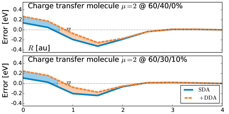
Figure 2: The error $\text{Err}(R)=\Delta{\cal E}_{\text{Hxc}}^{\rm approx}-\Delta{\cal E}_{\text{Hxc}}^{\rm exact}$ in excitation energies $\Delta{\cal E}={\cal E}-E_{\text{gs}}$, shown relative to the dissociation limit, $\text{Err}(R=4)$. Shown are 60/40/0% (top) and 60/30/10% (bottom) mixtures for the charge transfer case. We report both the pure state-driven only approximation (SDA) and the SD term plus the DD approximation (+DDA). Shaded regions indicate where including the DD approximation improves on the SD-only case (orange), or worsens it (blue). The diamond indicates the equilibrium interatomic distance.

So far we have been concerned with exact quantities. But for applications, it is essential to derive approximations. For a proof-of-principle demonstration, let us focus on charge transfers in 1D molecules. We approximate the SD terms using available ingredients for our 1D model – working in 3D would let us generate a variety of forms by tapping into the existing DFT zoo. The reported approximations use numerically exact KS densities $n_{s,\kappa}$.

We generate a SDA by combining the ensemble exact Hx results with a local spin density approximation (LSDA) for correlation, parametrised for the 1D soft-Coulomb potential Helbig et al. (2011); Wagner et al. (2012); Cas (2017). But we adapt the LSDA according to the formalism laid out by Becke, Savin and Stoll Becke et al. (1995) – which is useful for dealing with multiplets. Full details are provided in the Supplementary material.

The key point to be addressed here is the approximation for the DD terms (DDA). As far as charge transfer are concerned, intuition suggests that an electrostatic model may work well for a first DDA. Thus, we propose ${\cal E}_{\text{c}}^{{\text{DDA}}}=\sum_{\kappa}w_{\kappa}\big{\{}E_{\text{H}}[n_{\kappa}\rightarrow\tilde{n}_{\kappa}]-E_{\text{H}}[n_{s,\kappa}]\big{\}}$. This expression involves the KS densities $n_{s,\kappa}$ and $\tilde{n}_{\kappa}=S_{\kappa}n_{s,\kappa}[1+a\Delta n_{s,\kappa}+b\Delta n_{s,\kappa}^{2}]$ which accounts for the fact that in real situations we may not access the exact $n_{\kappa}$. Here, $S_{\kappa}$ is chosen to ensure the correct number of electrons, and the term $\Delta n_{s,\kappa}=n_{s,\kappa}-n$ (i.e., the deviation of the state density $n_{s,\kappa}$ from the full ensemble density $n$), ensures that the correction is zero in the case of a pure state. Parameters $a=-0.28$ and $b=0.12$ are found via optimization. Additional information on our DDA, including comparisons with the exact DD term, are provided in the Supplementary material.

Figure 2 shows errors in our approximations for the 60/30/10% case from earlier, and a 60/40/0% case without singlet excitations. Although the proposed approximation neglects both kinetic and x-like contributions [see eq. (9)], its performance is remarkably good. Including the DDA improves results for almost all chemically relevant $R$ (see orange shading).

Summary and outlook: Correlations in ensemble density functional theory (EDFT) are more than the simple sum of their parts. They naturally divide into state-driven (SD) and density-driven (DD) contributions, the former being amenable to direct translation of existing DFT approximations, and the latter being a unique property of ensembles. In prototypical ensembles of excited states, DD correlations account for up to 30% of the overall correlation energy. Therefore, accurate approximation of the correlation energy requires simultaneous consideration of the SD and DD components.

A simple approximation to the DD correlations was devised and evaluated in model situations. Thus, accounting for both SD and DD correlations was shown to be both feasible and promising to prompt progress in EDFT. Development of general approximations, extension to deal with systems that may challenge our simplifying “strong adiabatic” assumption, and generalization of key concepts and procedures presented here to other ensembles Perdew et al. (1982); Gould and Dobson (2013); Senjean and Fromager (2018); Deur and Fromager (2019) are being pursued.

References

- Hohenberg and Kohn (1964) P. Hohenberg and W. Kohn, Phys. Rev. 136, B864 (1964).
- Kohn and Sham (1965) W. Kohn and L. J. Sham, Phys. Rev. 140, A1133 (1965).
- Jones (2015) R. O. Jones, Rev. Mod. Phys. 87, 897 (2015).
- Matsika and Krylov (2018) S. Matsika and A. I. Krylov, Chem. Rev. 118, 6925 (2018).
- Runge and Gross (1984) E. Runge and E. K. Gross, Phys. Rev. Lett. 52, 997 (1984).
- Casida and Huix-Rotllant (2012) M. E. Casida and M. Huix-Rotllant, Annu. Rev. Phys. Chem. 63, 287 (2012).
- Ullrich and Tokatly (2006) C. A. Ullrich and I. V. Tokatly, Phys. Rev. B 73, 235102 (2006).
- Maitra (2017) N. T. Maitra, J. Phys.: Cond. Matter 29, 423001 (2017).
- Theophilou (1979) A. K. Theophilou, Journal of Physics C: Solid State Physics 12, 5419 (1979).
- Gross et al. (1988a) E. K. U. Gross, L. N. Oliveira, and W. Kohn, Phys. Rev. A 37, 2805 (1988a).
- Gross et al. (1988b) E. K. U. Gross, L. N. Oliveira, and W. Kohn, Phys. Rev. A 37, 2809 (1988b).
- Oliveira et al. (1988) L. N. Oliveira, E. K. U. Gross, and W. Kohn, Phys. Rev. A 37, 2821 (1988).
- Filatov and Shaik (1999) M. Filatov and S. Shaik, Chem. Phys. Lett. 304, 429 (1999).
- Filatov et al. (2015) M. Filatov, M. Huix-Rotllant, and I. Burghardt, J. Chem. Phys. 142, 184104 (2015).
- Filatov (2015) M. Filatov, WIREs Comput. Mol. Sci. 5, 146 (2015).
- Filatov (2016) M. Filatov, “Ensemble DFT approach to excited states of strongly correlated molecular systems,” in Density-Functional Methods for Excited States, edited by N. Ferré, M. Filatov, and M. Huix-Rotllant (Springer International Publishing, Cham, 2016) pp. 97–124.
- Franck and Fromager (2014) O. Franck and E. Fromager, Mol. Phys. 112, 1684 (2014).
- Deur et al. (2017) K. Deur, L. Mazouin, and E. Fromager, Phys. Rev. B 95, 035120 (2017).
- Pribram-Jones et al. (2014a) A. Pribram-Jones, Z.-h. Yang, J. R. Trail, K. Burke, R. J. Needs, and C. A. Ullrich, J. Chem. Phys. 140 (2014a).
- Yang et al. (2014) Z.-h. Yang, J. R. Trail, A. Pribram-Jones, K. Burke, R. J. Needs, and C. A. Ullrich, Phys. Rev. A 90, 042501 (2014).
- Yang et al. (2017) Z.-h. Yang, A. Pribram-Jones, K. Burke, and C. A. Ullrich, Phys. Rev. Lett. 119, 033003 (2017).
- Gould et al. (2018) T. Gould, L. Kronik, and S. Pittalis, J. Chem. Phys. 148, 174101 (2018).
- Sagredo and Burke (201) F. Sagredo and K. Burke, J. Chem. Phys. 149, 134103 (201).
- Ghosh et al. (2018) S. Ghosh, P. Verma, C. J. Cramer, L. Gagliardi, and D. G. Truhlar, Chem. Rev. (2018).
- Kim et al. (2013) M.-C. Kim, E. Sim, and K. Burke, Phys. Rev. Lett. 111, 073003 (2013).
- Gould and Pittalis (2017) T. Gould and S. Pittalis, Phys. Rev. Lett. 119, 243001 (2017).
- Perarnau-Llobet et al. (2015) M. Perarnau-Llobet, K. V. Hovhannisyan, M. Huber, P. Skrzypczyk, N. Brunner, and A. Acín, Phys. Rev. X 5, 041011 (2015).
- Deur and Fromager (2019) K. Deur and E. Fromager, J. Chem. Phys 150, 094106 (2019).
- Levy and Nagy (1999) M. Levy and A. Nagy, Phys. Rev. Lett. 83, 4361 (1999).
- Ayers et al. (2015) P. W. Ayers, M. Levy, and A. Nagy, The Journal of Chemical Physics 143, 191101 (2015).
- Pastorczak and Pernal (2014) E. Pastorczak and K. Pernal, J. Chem. Phys. 140, 18A514 (2014).
- Pribram-Jones et al. (2014b) A. Pribram-Jones, Z.-h. Yang, J. R. Trail, K. Burke, R. J. Needs, and C. A. Ullrich, J. Chem. Phys. 140, 18A541 (2014b).
- Gidopoulos et al. (2002) N. I. Gidopoulos, P. G. Papaconstantinou, and E. K. U. Gross, Phys. Rev. Lett. 88, 033003 (2002).
- Kraisler and Kronik (2013) E. Kraisler and L. Kronik, Phys. Rev. Lett. 110, 126403 (2013).
- Gould and Toulouse (2014) T. Gould and J. Toulouse, Phys. Rev. A 90 (2014).
- Helbig et al. (2011) N. Helbig, J. I. Fuks, M. Casula, M. J. Verstraete, M. A. Marques, I. Tokatly, and A. Rubio, Phys. Rev. A 83, 032503 (2011).
- Wagner et al. (2012) L. O. Wagner, E. Stoudenmire, K. Burke, and S. R. White, Phys. Chem. Chem. Phys. 14, 8581 (2012).
- Cas (2017) (2017), private communication from Michele Casula.
- Becke et al. (1995) A. Becke, A. Savin, and H. Stoll, Theor. Chim. Acta 91, 147 (1995).
- Perdew et al. (1982) J. P. Perdew, R. G. Parr, M. Levy, and J. L. Balduz, Phys. Rev. Lett. 49, 1691 (1982).
- Gould and Dobson (2013) T. Gould and J. F. Dobson, J. Chem. Phys. 138, 014103 (2013).
- Senjean and Fromager (2018) B. Senjean and E. Fromager, Phys. Rev. A 98, 022513 (2018).