Energy evolution and the Bose-Einstein enhancement for double gluon densities

E.  Gotsman gotsman@post.tau.ac.il Department of Particle Physics, School of Physics and Astronomy, Raymond and Beverly Sackler Faculty of Exact Science, Tel Aviv University, Tel Aviv, 69978, Israel    E.  Levin leving@post.tau.ac.il, eugeny.levin@usm.cl Department of Particle Physics, School of Physics and Astronomy, Raymond and Beverly Sackler Faculty of Exact Science, Tel Aviv University, Tel Aviv, 69978, Israel Departemento de Física, Universidad Técnica Federico Santa María, and Centro Científico-
Tecnológico de Valparaíso, Avda. Espana 1680, Casilla 110-V, Valparaíso, Chile
Abstract

In this paper we show that Bose-Einstein enhancement generates strong correlations which in the BFKL evolution, increase with energy. This increase leads to double gluon densities ( $\Phi$), which are much larger than the product of the single gluon densities ($\phi$). However, numerically, it turns out that the ratio $\Phi/\phi^{2}\propto\left(1/x\right)^{\delta_{2}}$ with $\delta_{2}\sim\bar{\alpha}_{S}/\left(N^{2}_{c}-1\right)^{2/3}\,\,\ll\,\,1$, and so we do not expect a large correction for the experimental accessible range of energies. However, for $N_{c}=3$, $\delta_{2}=0.07\Delta_{\rm BFKL}$ , where $\Delta_{\rm BFKL}$ denotes the intercept of the BFKL Pomeron, and thus we can anticipate a substantial increase for the range of rapidities $Y\sim 20$. We show that all $1/(N^{2}_{c}-1)$ corrections to the double gluon densities stem from Bose-Einstein enhancement.

BDGLAP evolution, double gluon distributions, Bose-Einstein correlations
pacs:
12.38.Cy, 12.38g,24.85.+p,25.30.Hm
preprint: TAUP - 3032/18

I Introduction

For a long time the double parton distribution functions (DPDFs) and their DGLAP evolution*** Dokshitzer, Gribov, Lipatov, Altarelli and Parisi (DGLAP) equationDGLAP describes the evolution in $\ln(Q^{2})$, where $Q$ is the hardest transverse momentum in the process, assuming that $\bar{\alpha}_{S}\ln(Q^{2})\sim 1$ but $\bar{\alpha}_{S}\ll 1$ and $\bar{\alpha}_{S}\,\ln(1/x)\ll 1$. This evolution was generalized for double parton distributions in Refs.Shelest:1982dg ; Zinovev:1982be ; Snigirev:2003cq ; Korotkikh:2004bz ; Gaunt:2009re ; Blok:2010ge have been of interest to the theoretical high energy community, and has been discussed in detail Shelest:1982dg ; Zinovev:1982be ; Snigirev:2003cq ; Korotkikh:2004bz ; Gaunt:2009re ; Blok:2010ge ; Ellis:1982cd ; Bukhvostov:1985rn ; LLS ; LALE ; Ceccopieri:2010kg ; Diehl:2011tt ; Gaunt:2011xd ; Ryskin:2011kk ; Bartels:2011qi ; Blok:2011bu ; Diehl:2011yj ; Luszczak:2011zp ; Manohar:2012jr ; Ryskin:2012qx ; Gaunt:2012dd ; Blok:2013bpa ; vanHameren:2014ava ; Maciula:2014pla ; Snigirev:2014eua ; Golec-Biernat:2014nsa ; Gaunt:2014rua ; Harland-Lang:2014efa ; Blok:2014rza ; Maciula:2015vza ; Diehl:2015bca . On the other hand the BFKL evolution The Balitsky, Fadin, Kuraev and Lipatov (BFKL) equationBFKL is written for evolution in $x$ (the energy scale of the process) assuming that $\bar{\alpha}_{S}\,\ln(1/x)\sim 1$ but $\bar{\alpha}_{S}\,\ll\,1$ and $\bar{\alpha}_{S}\ln(Q^{2})\,\ll\,1$. This evolution has been considered in Ref.MUPA ; PESCH ; LELU1 ; LELU2 ; LELULOOP for the double gluon densities. and related to them the double gluon densities (transverse momentum distributions(TMD2s)) have attracted less interest of the theorists, in spite of the fact, that they give the simplest way to estimate the possible correlations in the QCD parton cascade at high energies, where experimental observations of the double parton interactions Akesson:1986iv ; Abe:1997bp ; Abe:1997xk ; Abazov:2009gc ; Aad:2013bjm ; Chatrchyan:2013xxa ; Aad:2014rua were made.

In this paper we re-visit the evolution equation in the BFKL kinematic region of small $x$, where partons are either gluons or colorless dipoles. In the coordinate representation we use colorless dipoles as partons, while in the momentum representation, it is more convenient to discuss the parton cascade in terms of gluons. This evolution equation was written in Ref.MUPA (see also Refs.PESCH ) for the double gluon densities $\Phi\left(x_{1},p_{1,T};x_{2},p_{2,T}\right)\equiv\Phi\left(Y-y_{1},p_{1,T};Y-y_{2},p_{2,T}\right)$ with respect to rapidity ($Y$) of the initial hadron (projectile). Note that we use notation $\Phi\left(x_{1},p_{1,T};x_{2},p_{2,T}\right)$ for the double gluon density, and $\phi\left(x,p_{T}\right)$ for the single gluon density. $x_{i}$ is the fraction of energy of the gluon ‘i’ while $p_{i,T}$ denotes its transverse momentum. In the reference frame where the initial hadron is fast moving $\ln(1/x_{i})=Y-y_{i}$, $Y$ denotes the rapidity of the projectile(hadron) and $y_{i}$ the rapidity of the parton $i$. This evolution answers the question, what are the multiplicities of two colorless dipoles in one dipole, that moves with rapidity $Y$. We believe that in the spirit of the BFKL evolution we need to answer a different question, what is the multiplicity of two gluons with rapidities $y_{1}$ and $y_{2}$, if we know their multiplicities at $y_{1}=y^{0}_{1}$ and $y_{2}=y^{0}_{2}$. Therefore, the first goal of our paper is re-write the evolution equation in a convenient form to answer this question. It turns out that such evolution has been discussed in Refs.LELU1 ; LELU2 ; LELULOOP in the framework of the CGC approach (see Ref.KOLEB for the review of this approach). The evolution equations have been derived in these papers in the desired form, for $y_{1}=y_{2}$. It was shown, that it is not necessary to take into account the non-linear corrections for the double (and multi) gluons densities, and that the evolution equations reduce to the BFKL evolution. In Ref.LELULOOP this evolution is written taking into account the corrections of the order of $1/N^{2}_{c}$, where $N_{c}$ is the number of colors. The linear evolution equations for the double gluon density are closely related to the BKP equationsBKP for the scattering amplitude, and $1/N^{2}_{c}$ corrections to these equations have been discussed in Refs.BART1 ; BART2 ; LET2 ; BAWU ; BAEW ; AAKLL ; AKLL .

The second goal is to include the Bose-Einsten enhancement coming from the correlations of identical gluons, in the evolution. Bose-Einstein correlations have drawn considerable attention recently, since they give essential contributions to the azimuthal angle correlationsBEC1 ; BEC2 ; BEC3 ; BEC4 ; BEC5 ; BEC6 . It has been shown (see Ref.BEC4 for example) that the Bose-Einstein enhancement leads to a significant contribution to the measured angle correlations. We believe that this fact calls for a generalization of the evolution equation by taking into account this enhancement. We show that the Bose-Einstein enhancement is responsible for a term in the linear evolution which is suppressed as $1/\left(N^{2}_{c}-1\right)$, which has been found in Ref.LELULOOP . In other words, we state that all corrections of the order of $1/N^{2}_{c}$ in the evolution equations for the double gluon density, stem from the Bose-Einstein enhancement. In particular, the symmetry between the azimuthal angle $\varphi$ and the angle $\pi-\varphi$ does not appear. This symmetry, which is not based on the principle features of our CGC approach, reveals itself in the scattering amplitudes, but we do not find any indication of it in the double gluon densities. We wish to stress that, the Bose-Einstein corrections are closely related to the BKP equationsBKP and generate the energy behaviour of the twist four operator which increases as $s^{\Delta_{4}}$, with $\Delta_{4}>2\Delta_{2}$, $\Delta_{2}$ denotes the intercept of the BFKL Pomeron (see Refs.BART1 ; BART2 ; LET2 ).

We have discussed the Bose-Einstein enhancement for the DGLAP evolution GOLELAST , and have shown that it changes considerably, the high energy behavior of the DPDFs. In particular it turns out that the widely used assumption:

$$\Phi\left(x_{1},\boldsymbol{p}_{1,T}+\frac{1}{2}\boldsymbol{q}_{T};x_{2},\boldsymbol{p}_{2,T}-\frac{1}{2}\boldsymbol{q}_{T}\right)\,=\,F\left(q_{T}\right)\,\rho\left(x_{1},x_{2}\right)\,\phi\left(x_{1},p_{1,T}\right)\,\phi\left(x_{2},p_{3,T}\right)$$ (1)

does not hold, even at small $x_{1}$ and $x_{2}$, due the Bose-Einstein correlations In Ref.GBS2 ; GBS it is shown that Eq. (1) is a good approximation to the solution of the DGLAP evolution equation for the double parton distribution functions at small $x$ and large $p_{T}$, but this claim is only correct, when neglecting the contributions of the order of $1/(N^{2}_{c}-1)$..

Before describing the structure of the paper we would like to introduce the observables of interest: the parton density $\phi\left(x,p_{t},q_{T}\right)$ and the double parton density $\Phi\left(x_{1},\boldsymbol{p}_{1,T};x_{2},p_{2,T};\boldsymbol{q}_{T}\right)$. The single gluon density characterizes the multiplicity of gluons with fraction of energy $x$ and transverse momentum $\boldsymbol{p}_{T}$ at $q_{T}=0$, and it can be written as follows

$\displaystyle\phi\left(x,\boldsymbol{p}_{T},\boldsymbol{q}_{T};b\right)\,$ $\displaystyle=$ $\displaystyle\,\,\sum^{\infty}_{n=1}\,\int\,\prod^{n}_{i=1}\frac{dx_{i}}{x_{i}}\,d^{2}k_{i,T}\,\sum_{c_{i}}\,\langle\Omega^{+}_{n}|\Psi^{*}\left(\{x_{i},\boldsymbol{k}_{i,T};c_{i}\}\right)$ (2)
$\displaystyle\,\Bigg{\{}a^{+}(x,\boldsymbol{p}_{T}+\frac{1}{2}\boldsymbol{q}_{T};b)\,\,\,a(x,\boldsymbol{p}_{T}-\frac{1}{2}\boldsymbol{q}_{T};b)\Bigg{\}}\,\Psi\left(\{x_{i},\boldsymbol{k}_{i,T};c_{i}\},\right)|\Omega_{n}\rangle$

where $\Psi$ denotes the partonic wave function of the fast hadron, $|\Omega_{n}\rangle=\prod^{n}_{i}\,a^{+}(x_{i},\boldsymbol{k}_{i,T},c_{i})|0\rangle$ ($|0\rangle$ denotes the vacuum state) and $a^{+}(x_{i},\boldsymbol{k}_{i,T},c_{i})$ and $a(x_{i},\boldsymbol{k}_{i,T},c_{i})$ denote the creation and annihilation operators for partons (gluons for small $x_{i}$) with fraction of energy $x_{i}$, transverse momentum $\boldsymbol{k}_{i,T}$ and color $c_{i}$. The produced gluon has longitudinal momentum $x$ and transverse momentum $\boldsymbol{p}_{T}$, while $b$ indicates its color.

The double transverse momentum densities describe the number of gluons with $(x_{1},p_{1,T})$ and $(x_{2},p_{2,T})$ in the parton cascade, and it can be written with the aid of the wave function of the produced gluon $\Psi\left(\{x_{i},k_{i,T}\}\right)$ as follows

$\displaystyle\Phi\left(x_{1},\boldsymbol{p}_{1,T};x_{2},\boldsymbol{p}_{2,T};\boldsymbol{q}_{T};b,c\right)\,=\,\,\sum^{\infty}_{n=2}\,\int\,\prod^{n}_{i=1}\frac{dx_{i}}{x_{i}}\,d^{2}k_{i,T}\,\sum_{c_{i}}\,\langle\Omega^{+}_{n}|\Psi^{*}\left(\{x_{i},\boldsymbol{k}_{i,T};c_{i}\}\right)$
$\displaystyle\,\Bigg{\{}a^{+}(x_{1},\boldsymbol{p}_{1,T}+\frac{1}{2}\boldsymbol{q}_{T};b)\,a^{+}(x_{2},\boldsymbol{p}_{2,T}-\frac{1}{2}\boldsymbol{q}_{T};c)\,a(x_{2},\boldsymbol{p}_{2,T}+\frac{1}{2}\boldsymbol{q}_{T};c)\,a(x_{1},\boldsymbol{p}_{1,T}-\frac{1}{2}\boldsymbol{q}_{T};b)\Bigg{\}}\Psi\left(\{x_{i},\boldsymbol{k}_{i,T};c_{i}\}\right)|\Omega_{n}\rangle$ (3)

The paper is organized as follows: In the next section we discuss the BFKL evolution of the double gluon density in the region of low $x$. For completeness of presentation we review the derivation of the evolution equations for the double gluon densities which was done in Refs.LELU1 ; LELU2 ; LELULOOP in the framework of the dipole approachMUDI . In spite of the fact that this derivation is only valid for $y_{1}=y_{2}$, it shows that these evolution equations are linear BFKL equations which are not affected by non-linear shadowing corrections. In section 3 we re-derive the BFKL equations for the double gluon densities directly in the momentum representation. In this representation, we generalize the equation for the case of $y_{1}\neq y_{2}$ and re-write the equations in the form which is suitable for taking into account the Bose-Einstein enhancement (BEE). In this section we find the solutions to the equations without BEE. The interference diagrams that are responsible for the BEE, are discussed in section 4. In section 5 the evolution equations with BEE are proposed, and we find that $\Phi/\phi^{2}\propto\left(1/x\right)^{\delta_{2}}$ with $\delta_{2}\sim\bar{\alpha}_{S}/\left(N^{2}_{c}-1\right)^{2/3}$. Section 5 is devoted to a discussion of the energy behavior of the double gluon densities. In the conclusions we discuss our main results.

II BFKL evolution of double dipole densities in the CGC approach.

In this section we discuss the evolution equation for the double gluon densities in the framework of the CGC approach. As mentioned this equation has been derived in Refs.LELU1 ; LELU2 ; LELULOOP , here we give a brief review both for completeness of the presentation, and to display the main features of the multi gluon densities, which are not the main subject of these papers. The partonic wave function can be expanded as the sum of Fock states with fixed multiplicity of partons (colorless dipoles):

$$\Psi\Big{(}\{\boldsymbol{r}_{i},\boldsymbol{b}_{i}\}\Big{)}\,\,=\,\,\sum_{n}\,\alpha_{n}|\Omega_{n}\rangle$$ (4)

The colorless dipole is characterized by two variables: its size $\boldsymbol{r}_{i}$ and its impact parameter $\boldsymbol{b}_{i}$. However, in this paper we will sometimes use a different set of variables: $\boldsymbol{x}_{i}$ for the position of the quark and $\boldsymbol{y}_{i}$ for the position of the anti-quark in the dipole. One can see that $\boldsymbol{r}_{i}\,=\boldsymbol{x}_{i}\,-\,\boldsymbol{y}_{i}$ and $\boldsymbol{b}_{i}\,=\,\frac{1}{2}\left(\boldsymbol{x}_{i}\,+\,\boldsymbol{y}_{i}\right)$. $\alpha_{n}^{2}$ is the probability to find $n$ dipoles with the same value of rapidity $Y$ :

$$\alpha^{2}_{n}\,=\,P_{n}\left(Y;\{\boldsymbol{r}_{i},\boldsymbol{b}_{i}\}\right)$$ (5)

The QCD cascade can be written as the linear functional equation for the following functionalMUDI ; LELU1 :

$$Z\left(\tilde{Y}=Y-y;\,[u_{i}]\right)\,\,\equiv\,\,\sum_{n=1}\,\int\,\,P_{n}\left(Y\,;\,\{\boldsymbol{r}_{i},\boldsymbol{b}_{i}\}\right)\,\,\prod^{n}_{i=1}\,u(r_{i},b_{i})\,d^{2}\,r_{i}\,d^{2}\,b_{i}$$ (6)

where $u(r_{i},b_{i})\equiv u_{i}$ is an arbitrary function of $r_{i}$ and $b_{i}$ and $y=y_{1}=y_{2}$. It follows immediately from Eq. (5) that the functional obeys the condition: at $u_{i}\,=\,1$

$$Z\left(\tilde{Y}\,;\,[u_{i}=1]\right)\,\,=\,\,1\,.$$ (7)

The physical meaning of Eq. (7) is that the sum over all probabilities is one.

II.1 Balitsky-Kovchegov parton cascade

To write the evolution equation, we need to specify the QCD processes with color dipoles. The parton cascade that leads to the Balitsky-Kovchegov non-linear equation for the scattering amplitude, stems from the process of the decay of one dipole to two dipoles, which gives the main contribution at the leading order of perturbative QCD at large $N_{c}$MUDI . The probability of this decay is equal to

$$P_{1\to 2}\left(|\boldsymbol{r}_{1}+\boldsymbol{r}_{2}|\to r_{1}+r_{2}\right)\,\,=\,\,\frac{\bar{\alpha}_{S}}{2\,\pi}\,\frac{\left(\boldsymbol{r}_{1}+\boldsymbol{r}_{2}\right)^{2}}{r^{2}_{1}\,r^{2}_{2}}$$ (8)

Bearing Eq. (8) in mind, we can write the linear equation for $Z$:

$$\,\frac{\partial\,Z}{\bar{\alpha}_{S}\,\partial\,\tilde{Y}}\,\,=\,\,-\,\,\int\,d^{2}r\,d^{2}b\,\,V_{1\rightarrow 1}(\boldsymbol{r},\,\boldsymbol{b},\,[u])\,\,Z\,\,+\,\,\int\,\,d^{2}\,r\,d^{2}\,r^{\prime}\,d^{2}b\,\,V_{1\rightarrow 2}(\boldsymbol{r},\,\boldsymbol{r}^{\prime},\,\boldsymbol{b},\,[u])\,\,Z\,$$ (9)

with the definitions

$$V_{1\rightarrow 1}(\boldsymbol{r},\,\boldsymbol{b},\,[u])\,\,=\,\,\,\,\omega(r)\,\,u(\boldsymbol{r},\,\boldsymbol{b})\,\,\frac{\delta}{\delta u(\boldsymbol{r},\boldsymbol{b})}~{}\mbox{with}~{}\omega\left(r\right)\,\,=\,\,\int d^{2}r^{\prime}\,P_{1\to 2}\left(r\to r^{\prime}+|\boldsymbol{r}-\boldsymbol{r}^{\prime}|\right)\,\,=\,\,\frac{\bar{\alpha}_{S}}{2\pi}\int d^{2}r^{\prime}\frac{r^{2}}{r^{\prime 2}\,\left(\boldsymbol{r}-\boldsymbol{r}^{\prime}\right)^{2}}$$ (10)

and

$$V_{1\rightarrow 2}(\boldsymbol{r},\,\boldsymbol{r}^{\prime},\,\boldsymbol{b},\,[u])\,\,=\,\,\frac{\bar{\alpha}_{S}}{2\,\pi}\,\,\frac{r^{2}}{r^{\prime 2}\,(\boldsymbol{r}-\boldsymbol{r}^{\prime})^{2}}\,\,\,u\left(\boldsymbol{r}^{\prime},\,\boldsymbol{b}\,+\,\frac{1}{2}(\boldsymbol{r}\,-\,\boldsymbol{r}^{\prime})\right)\,\,u\left(\boldsymbol{r}\,-\,\boldsymbol{r}^{\prime},\,\boldsymbol{b}\,-\,\frac{1}{2}\boldsymbol{r}\right)\,\,\frac{\delta}{\delta u(\boldsymbol{r},\,\boldsymbol{b})}\,.$$ (11)

The functional derivative with respect to $u(r,b)$, plays the role of an annihilation operator for a dipole of size $r$, at impact parameter $b$. The multiplication by $u(r,b)$ corresponds to a creation operator for this dipole. Therefore,Eq. (9) is a typical cascade equation in which the first term describes the depletion of the probability due to splitting into $n+1$ dipoles, while the second term is responsible for the growth due to splitting of $(n-1)$ dipoles into $n$ dipoles. From Eq. (6), one can see that the multi dipole density $\rho^{(n)}\left(Y-Y_{0};\{\boldsymbol{r}_{i},\boldsymbol{b}_{i}\}\right)$ can be found as follows

$\displaystyle\rho^{(n)}\left(Y-y;\{\boldsymbol{r}_{i},\boldsymbol{b}_{i}\}\right)\,$ $\displaystyle=$ $\displaystyle\,\frac{1}{n!}\,\prod^{n}_{i=1}\,\frac{\delta}{\delta u_{i}}\,Z\left(Y\,-\,y;\,[u_{i}]\right)|_{u=1}\,\,$
$\displaystyle=$ $\displaystyle\,\,\sum^{\infty}_{k=n}\frac{k!}{(k-n)!\,n!}\,\int P_{k}\left(Y-y\,;\,\boldsymbol{r}_{1},\boldsymbol{b}_{1},\dots,\boldsymbol{r}_{n},\boldsymbol{b}_{n},\{\{\boldsymbol{r}_{i},\boldsymbol{b}_{i}\}\right)\,\,\prod^{k}_{i=n+1}\,\,d^{2}\,r_{i}\,d^{2}\,b_{i}$

which gives the probability of finding $n$-dipoles with the given kinematics.

From Eq. (9) we obtain

$\displaystyle\frac{\partial\,\rho^{(n)}(\tilde{Y};\boldsymbol{r}_{1},\boldsymbol{b}_{1}\,\ldots\,,\boldsymbol{r}_{n},\boldsymbol{b}_{n})}{\bar{\alpha}_{S}\,\partial\,\tilde{Y}}\,\,=\,\,-\,\sum_{i=1}^{n}\,\,\omega(r_{i})\,\,\rho^{(n)}(Y-y;\boldsymbol{r}_{1},\boldsymbol{b}_{1}\,\ldots\,,\boldsymbol{r}_{n},\boldsymbol{b}_{n})\,\,$ (13)
$\displaystyle+2\,\sum_{i=1}^{n}\,\int\,\frac{d^{2}\,r^{\prime}}{2\,\pi}\,\frac{r^{\prime 2}}{r^{2}_{i}\,(\boldsymbol{r}_{i}\,-\,\boldsymbol{r}^{\prime})^{2}}\,\rho^{(n)}(Y-y;\ldots\,\boldsymbol{r}^{\prime},\boldsymbol{b}_{i}-\frac{1}{2}\boldsymbol{r}^{\prime},\dots)+\sum_{i=1}^{n-1}\,\frac{(\boldsymbol{r}_{i}+\boldsymbol{r}_{n})^{2}}{(2\,\pi)\,r^{2}_{i}\,r^{2}_{n}}\,\rho^{(n-1)}(Y-y;\dots,\boldsymbol{r}_{i}\,+\,\boldsymbol{r}_{n},\boldsymbol{b}_{in},\dots)$

For $\rho^{(2)}$ we have

$\displaystyle\frac{\partial\,\rho^{(2)}(\tilde{Y};\boldsymbol{r}_{1},\boldsymbol{b}_{1};\boldsymbol{r}_{2},\boldsymbol{b}_{2})}{\bar{\alpha}_{S}\,\partial\,\tilde{Y}}\,\,=\,\,-\,\sum_{i=1}^{2}\,\,\omega(r_{i})\,\,\rho^{(2)}(\tilde{Y};\boldsymbol{r}_{1},\boldsymbol{b}_{1};\boldsymbol{r}_{2},\boldsymbol{b}_{2})\,\,$ (14)
$\displaystyle+2\,\Bigg{(}\,\int\,\frac{d^{2}\,r^{\prime}}{2\,\pi}\,\frac{r^{\prime 2}}{r^{2}_{1}\,(\boldsymbol{r}_{1}\,-\,\boldsymbol{r}^{\prime})^{2}}\,\rho^{(2)}(\tilde{Y};\boldsymbol{r}^{\prime},\boldsymbol{b}_{1}-\frac{1}{2}\boldsymbol{r}^{\prime},\boldsymbol{r}_{2},\boldsymbol{b}_{2}\dots)\,+\,\Big{(}1\,\leftrightarrows\,2\Big{)}\Bigg{)}\,\,+\,\,\frac{(\boldsymbol{r}_{1}+\boldsymbol{r}_{2})^{2}}{(2\,\pi)\,r^{2}_{1}\,r^{2}_{2}}\,\rho^{(1)}(\tilde{Y};\boldsymbol{r}_{i}\,+\,\boldsymbol{r}_{2},\boldsymbol{b}_{12})$

There are two main features of the equation: (i) there are no non-linear corrections, and (ii) we have two contributions: BFKL evolution of $\rho^{(2)}$ and the contribution to $\rho^{(2)}$ from single parton showers. This structure is the same as in the DGLAP evolution (see Refs.Shelest:1982dg ; Zinovev:1982be ; Snigirev:2003cq ; Korotkikh:2004bz ; Gaunt:2009re ; Blok:2010ge ).

II.2 $1/N^{2}_{c}$ corrections to the Balitsky-Kovchegov cascade

Refer to caption
Figure 1: A graphical representation of the decay of two dipoles to three dipoles: $x_{12}+x_{34}\,\to\,x_{23}+x_{14}\,\to x_{z2}\,+\,x_{3z}+x_{14}$. The lines of the same colors indicate the colorless dipole which decays in two dipoles due to emission of a gluon with coordinate $\boldsymbol{z}$.

In Ref.LELULOOP it is suggested to add the following term to Eq. (9):

$\displaystyle\int\prod_{i=1}^{2}d^{2}x_{i}\,d^{2}y_{i}\,d^{2}z\,\,\frac{1}{N^{2}_{c}-1}P_{1\to 2}\left(|\boldsymbol{x}_{2}-\boldsymbol{y}_{1}|\to\,|\boldsymbol{x}_{2}-\boldsymbol{z}|\,+\,|\boldsymbol{z}-\boldsymbol{y}_{1}|\right)$
$\displaystyle\times\,\,\Big{(}1-u\left(\boldsymbol{x}_{1},\boldsymbol{y}_{2}\right)\Big{)}\,\Big{(}u\left(\boldsymbol{x}_{2},\boldsymbol{y}_{1}\right)\,-\,u\left(\boldsymbol{z},\boldsymbol{y}_{1}\right)\,u\left(\boldsymbol{x}_{2},\boldsymbol{z}\right)\Big{)}\frac{\delta}{\delta u\left(\boldsymbol{x}_{1},\boldsymbol{y}_{1}\right)}\,\frac{\delta}{\delta u\left(\boldsymbol{x}_{2},\boldsymbol{y}_{2}\right)}\,Z\left(Y,[u_{i}]\right)$ (15)

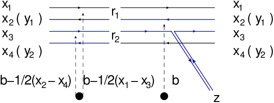
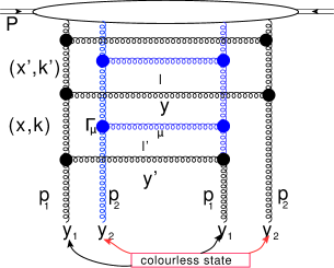
The process that is described by Eq. (II.2) is shown in Fig. 1. Indeed, if two dipoles consist of quarks and antiquarks with the same colors, the dipole, in which one quark from one dipole and the antiquark from another dipole, can create a different dipole which decays into $q,\bar{q}$ and a gluon. The term of Eq. (II.2) generates the$1/(N^{2}_{c}-1)$ corrections to Eq. (14) which have the following form:

$\displaystyle\frac{1}{N^{2}_{c}-1}\Bigg{\{}P_{1\to 2}\Big{(}(\boldsymbol{x}_{1},\boldsymbol{y}_{2})\to(\boldsymbol{x}_{1},\boldsymbol{y}_{1})\,+\,(\boldsymbol{x}_{2},\boldsymbol{y}_{1})\Big{)}\,\delta^{(2)}\left(\boldsymbol{x}_{2}-\boldsymbol{y}_{1}\right)\,\rho^{(1)}\left(\tilde{Y};\boldsymbol{x}_{2},\boldsymbol{y}_{2}\right)\,+\,P_{1\to 2}\Big{(}(\boldsymbol{x}_{2},\boldsymbol{y}_{1})\to(\boldsymbol{z},\boldsymbol{y}_{1})+(\boldsymbol{x}_{2},\boldsymbol{z})\Big{)}$
$\displaystyle\times\,\,\Bigg{(}\rho^{(2)}\left(\tilde{Y};\boldsymbol{x}_{1},\boldsymbol{y}_{2};\boldsymbol{z},\boldsymbol{y}_{1}\right)\,+\,\rho^{(2)}\left(\tilde{Y};\boldsymbol{x}_{1},\boldsymbol{y}_{2};\boldsymbol{x}_{2},\boldsymbol{z}\right)\,\,-\,\,\rho^{(2)}\left(\tilde{Y};\boldsymbol{x}_{1},\boldsymbol{y}_{2};\boldsymbol{x}_{2},\boldsymbol{y}_{1}\right)\Bigg{)}+\Big{(}1\,\leftrightarrows\,2\Big{)}\Bigg{\}}$ (16)

One can see that the structure of Eq. (II.2) is similar to that of Eq. (14): i.e. the production of two dipoles from the single parton cascade, and the evolution of the double density with a kernel which is different from Eq. (14), although it consists of the same elements. We need to re-write Eq. (14) with additional term of Eq. (II.2) in the momentum representation, to obtain the more familiar form of the double gluon density evolution equation. However, we chose a different strategy: we derive the equation directly in the momentum representation. First, we believe that we can relax the assumption that $y_{1}=y_{2}$ and second, we hope that this derivation will clarify the physical meaning of the additional term of Eq. (II.2).

We would like to stress that the derivation, which we have discussed, is very instructive for understanding the different contributions to the evolution due to the clear physics interpretation of the dipole approach in perturbative QCD.

III BFKL evolution without Bose-Einstein enhancement

III.1 Equations for $\bar{\alpha}_{S}|y_{2}-y_{1}|\,\gg\,\,1$.

In this section we re-write Eq. (14) in the momentum representation using two lessons from the derivation of the previous section. The double parton density is not affected by the shadowing (screening) corrections and obeys the linear BFKL equations, and the equation should match Eq. (14) at $y_{1}=y_{2}$.

In the BFKL region we consider that $\bar{\alpha}_{S}\,\ln\left(1/x_{i}\right)\,=\,Y-y_{i}\,\gg\,1$ while $\bar{\alpha}_{S}\ln(p_{i,T}^{2}/Q^{2}_{0})\,\ll\,1$, and $\bar{\alpha}_{S}\,\ll\,1$ and the evolution equations sum the contributions of the order of $\left(\bar{\alpha}_{S}\ln(1/x)\right)^{n}$ (leading log(1/x) approximation (LLA)).
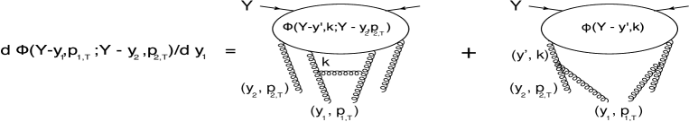
Refer to caption
Figure 2: The graphical representation of the evolution equation(see Eq. (17) and Eq. (18)).

In the region of small $x_{i}$ only a gluon can be produced KOLEB , and for the double gluon density we expect to have two equations of the following forms(see Fig. 2)

$\displaystyle\frac{\partial\Phi\left(Y-y_{1},p_{1,T};Y-y_{2},p_{2,T};q_{T}\right)}{\partial\,\left(Y-y_{1}\right)}\,\,$ $\displaystyle=$ $\displaystyle\,\,\bar{\alpha}_{S}\int\frac{d^{2}k_{T}}{2\pi}K\left(p_{1,T},k_{T};q_{T}\right)\,\Phi\left(Y-y_{1},k_{T};Y-y_{2},p_{2,T};q_{T}\right)\,$ (17)
$\displaystyle+$ $\displaystyle\,\,\bar{\alpha}_{S}\,\phi\left(Y-y^{\prime},\boldsymbol{p}_{1,T}+\boldsymbol{p}_{2,T}\right)\,\Gamma\left(p_{1},p_{2};y_{1},y_{2}\right);$
$\displaystyle\frac{\partial\Phi\left(Y-y_{1},p_{1,T};Y-y_{2},p_{2,T};q_{T}\right)}{\partial\,\left(Y-y_{2}\right)}\,\,$ $\displaystyle=$ $\displaystyle\,\,\bar{\alpha}_{S}\int\frac{d^{2}k_{T}}{2\pi}K\left(p_{2,T},k_{T};q_{T}\right)\,\Phi\left(Y-y_{1},p_{1,T};Y-y_{2},k_{T}\right)\,$ (18)
$\displaystyle+$ $\displaystyle\,\,\bar{\alpha}_{S}\,\phi\left(Y-y^{\prime},\boldsymbol{p}_{1,T}+\boldsymbol{p}_{2,T}\right)\,\Gamma\left(p_{1},p_{2};y_{2},y_{1}\right);$

where $K\left(p_{T},k_{T}\right)$ is the BFKL kernel which is equal to BFKL

$\displaystyle K\left(p_{T},k_{T};q_{T}\right)\,\,$ $\displaystyle=$ $\displaystyle\,\,\frac{1}{\left(\boldsymbol{p}_{T}\,-\,\boldsymbol{k}_{T}\right)^{2}}\Bigg{\{}\frac{\left(\boldsymbol{p}_{T}-\frac{1}{2}\boldsymbol{q}_{T}\right)^{2}}{\left(\boldsymbol{k}_{T}-\frac{1}{2}\boldsymbol{q}_{T}\right)^{2}}\,+\,\frac{\left(\boldsymbol{p}_{T}+\frac{1}{2}\boldsymbol{q}_{T}\right)^{2}}{\left(\boldsymbol{k}_{T}+\frac{1}{2}\boldsymbol{q}_{T}\right)^{2}}\Bigg{\}}\,-\,\frac{q^{2}_{T}}{\left(\boldsymbol{k}_{T}+\frac{1}{2}\boldsymbol{q}_{T}\right)^{2}\,\left(\boldsymbol{k}_{T}-\frac{1}{2}\boldsymbol{q}_{T}\right)^{2}}$
$\displaystyle-$ $\displaystyle\,\,\Bigg{\{}\omega_{G}\left(\boldsymbol{p}_{T}+\frac{1}{2}\boldsymbol{q}_{T}\right)\,+\,\omega_{G}\left(\boldsymbol{p}_{T}-\frac{1}{2}\boldsymbol{q}_{T}\right)\Bigg{\}}\,\delta^{(2)}\left(\boldsymbol{p}_{T}-\boldsymbol{k}\right)$ (19)
$\displaystyle\omega_{G}\left(p_{T}\right)$ $\displaystyle=$ $\displaystyle\,\,\frac{1}{2}\,p^{2}_{T}\int\frac{d^{2}k_{T}}{2\pi}\frac{1}{\left(\boldsymbol{p}_{T}\,-\,\boldsymbol{k}_{T}\right)^{2}\,k^{2}_{T}}$ (20)
$\displaystyle K\left(p_{T},k_{T};q_{T}=0\right)\,\,$ $\displaystyle=$ $\displaystyle\,\,\frac{2}{\left(\boldsymbol{p}_{T}\,-\,\boldsymbol{k}_{T}\right)^{2}}\frac{p^{2}_{T}}{k^{2}_{T}}-2\omega_{G}\left(p_{T}\right)\,\delta^{(2)}\left(\boldsymbol{p}_{T}-\boldsymbol{k}_{T}\right)$ (21)

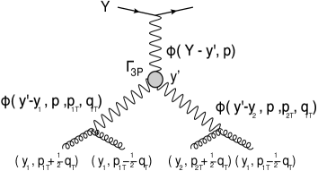
The non -homogenous term takes into account the possibility to produce two gluons from a single gluon cascade. The expression for these terms is written directly from the second diagram of Fig. 2. Function $\Gamma\left(\boldsymbol{p}_{1T},\boldsymbol{p}_{2T};y_{1},y_{2}\right)$ has to be found. It is clear that for $\bar{\alpha}_{S}|y_{2}-y_{1}|\,\gg\,\,1$ two emitted gluons in Fig. 2 with rapidities $y_{1}$ and $y_{2}$ can emit gluons, and the observed gluons will be amongst them. Therefore, the general diagram, which determines the non-homogenous term is the triple BFKL Pomeron diagram of Fig. 3-a.

Refer to caption Refer to caption
Fig. 3-a Fig. 3-b
Figure 3: Fig. 3-a:The graphical representation of the triple BFKL Pomeron diagrams. For simplicity we show the evolution at $q_{T}=0$. Fig. 3-b: the structure of the partonic wave function in the light-cone perturbative approach for the production of two gluons from the single parton cascade at $x_{1}=x_{2}$ ($y_{1}=y_{2}$). We denote by $D_{n}$ the dominator of the propagator for the state that has $n$-gluons.

This diagram can be written in the following general form

$$\Phi_{3{I\!\!P}}\left(Y,y_{1},y_{2};\boldsymbol{p}_{1,T},\boldsymbol{p}_{2,T},q_{T}\right)\,\,=\,\,\bar{\alpha}_{S}\int^{Y}_{y_{2}\,\geq\,y_{1}}\!\!\!\!\!\!\!\!\!\!\!\!\!dy^{\prime}\,d^{2}p_{T}\phi_{\rm pr}\left(Y-y^{\prime},p_{T}\right)\,\Gamma_{3{I\!\!P}}\left(p_{T}\right)\,\phi\left(y^{\prime}-y_{1},\boldsymbol{p}_{T},\boldsymbol{p}_{1,T},q_{T}\right)\,\phi\left(y^{\prime}-y_{2},\boldsymbol{p}_{T},\boldsymbol{p}_{2,T},q_{T}\right)$$ (22)

where $\Gamma_{3{I\!\!P}}$ denotes the triple BFKL Pomeron vertex which we will discuss below. The single gluon densities in Eq. (22) $\phi_{\rm pr}$ and $\phi$ are different, since $\phi_{\rm pr}$ is the density of the gluons in the projectile (hadron), while $\phi$ is the density of the gluons in the cascade of the single gluon with rapidity $Y-y^{\prime}$. This term in the evolution was considered for the first time in Ref.MUPA . We refer our readers to this paper or more detail.

The contributions of this diagram to the evolution equation have the following form for $y_{2}>y_{1}$:

$\displaystyle 1.\,\,\frac{\partial\Phi_{3{I\!\!P}}\left(Y,y_{1},y_{2};\boldsymbol{p}_{1,T},\boldsymbol{p}_{2,T},q_{T}\right)}{\partial y_{1}}$ $\displaystyle=$ $\displaystyle\bar{\alpha}_{S}\int^{Y}_{y_{2}\,\geq\,y_{1}}\!\!\!\!\!\!\!\!\!\!\!\!\!\!\!\!dy^{\prime}\,d^{2}p_{T}\,\phi_{\rm pr}\left(Y-y^{\prime},p_{T}\right)\,\Gamma_{3{I\!\!P}}\left(p_{T}\right)\,\frac{\partial\phi}{\partial y_{1}}\left(y^{\prime}-y_{1},\boldsymbol{p}_{T},\boldsymbol{p}_{1,T},q_{T}\right)\,\phi\left(y^{\prime}-y_{2},\boldsymbol{p}_{T},\boldsymbol{p}_{2,T},q_{T}\right);$
$\displaystyle 2.\,\,\frac{\partial\Phi_{3{I\!\!P}}\left(Y,y_{1},y_{2};\boldsymbol{p}_{1,T},\boldsymbol{p}_{2,T},q_{T}\right)}{\partial y_{2}}$ $\displaystyle=$ $\displaystyle\bar{\alpha}_{S}\int^{Y}_{y_{2}\,\geq\,y_{1}}\!\!\!\!\!\!\!\!\!\!\!\!\!\!\!\!dy^{\prime}\,d^{2}p_{T}\,\phi_{\rm pr}\left(Y-y^{\prime},p_{T}\right)\,\Gamma_{3{I\!\!P}}\left(p_{T}\right)\,\phi\left(y^{\prime}-y_{1},\boldsymbol{p}_{T},\boldsymbol{p}_{1,T},q_{T}\right)\,\frac{\partial\phi}{\partial y_{2}}\left(y^{\prime}-y_{2},\boldsymbol{p}_{T},\boldsymbol{p}_{2,T},q_{T}\right)$ (23)
$\displaystyle+$ $\displaystyle\,\bar{\alpha}_{S}\,\int d^{2}p_{T}\,\phi_{\rm pr}\left(Y-y_{2},p_{T}\right)\,\Gamma_{3{I\!\!P}}\left(p_{T}\right)\phi\left(y_{2}-y_{1},\boldsymbol{p}_{T},\boldsymbol{p}_{1,T},q_{T}\right)\,\phi\left(0,\boldsymbol{p}_{T},\boldsymbol{p}_{2,T},q_{T}\right);$

From Eq. (17) and Eq. (18) one can see that the first term in the both equations is included in the first terms of the evolution equations since

$$\frac{\partial\phi}{\partial y_{i}}\left(y^{\prime}-y_{i},\boldsymbol{p}_{T},\boldsymbol{p}_{2,T},q_{T}\right)\,\,=\,\,-\bar{\alpha}_{S}\,\int d^{2}k_{T}\,\,K\left(p_{i,T},k_{T};q_{T}\right)\,\,\phi\left(y^{\prime}-y_{i},\boldsymbol{p}_{T},\boldsymbol{p}_{2,T},q_{T}\right)$$ (24)

We also see that Eq. (23) does not generate the non-homogenous term in Eq. (17) if $y_{1}\,<\,y_{2}$, in the case which we consider here: $y_{2}>y_{1}$. We need to specify the triple BFKL Pomeron vertex and $\phi\left(0,\boldsymbol{p}_{T},\boldsymbol{p}_{2,T},q_{T}\right)$ in Eq. (23). Actually

$$\phi\left(0,\boldsymbol{p}_{T},\boldsymbol{p}_{2,T},q_{T}\right)\,\,=\,\,\delta^{(2)}\left(\boldsymbol{p}_{T}-\boldsymbol{p}_{2,T}\right)$$ (25)

In the diagram of Fig. 3-a the triple Pomeron vertex enters with the momentum transferred along the upper Pomeron being equal to zero. We believe that we can find this vertex directly from the non-linear Balitsky-Kovchegov evolution equationBK for the scattering dipole amplitude:

$\displaystyle\frac{\partial N\left(Y;x_{12},b\right)}{\partial\,Y}\,\,$ $\displaystyle=$ $\displaystyle\,\,\bar{\alpha}_{S}\,\int\frac{d^{2}x_{3}}{\pi}\,\frac{x^{2}_{12}}{x^{2}_{13}\,x^{2}_{23}}\Big{\{}N\left(Y;x_{13},\boldsymbol{b}-\frac{1}{2}\boldsymbol{x}_{23}\right)\,+\,N\left(Y;x_{23},\boldsymbol{b}-\frac{1}{2}\boldsymbol{x}_{13}\right)\,-\,N\left(Y;x_{12},b\right)\,\,$ (26)
$\displaystyle-$ $\displaystyle\,\,N\left(Y;x_{13},\boldsymbol{b}-\frac{1}{2}\boldsymbol{x}_{23}\right)\,N\left(Y;x_{23},\boldsymbol{b}-\frac{1}{2}\boldsymbol{x}_{13}\right)\Big{\}}$

where $x_{ik}\,=\,\boldsymbol{x}_{i}\,-\,\boldsymbol{x_{k}}$ and $b$ denotes the impact factor. Eq. (26) in the momentum representation, which we define as

$$N\left(Y;x_{12},b\right)\,\,=\,\,x^{2}_{12}\int\frac{d^{2}k_{T}}{2\pi}\,\frac{d^{2}q_{T}}{2\pi}e^{i\boldsymbol{x}_{12}\cdot\boldsymbol{k}_{T}\,\,+\,\,i\,\boldsymbol{b}\cdot\boldsymbol{q}_{T}}\,\phi\left(Y;k_{T},q_{T}\right)$$ (27)

has the following form:

$$\frac{\partial\phi\left(Y;k_{T},q_{T}=0\right)}{\partial Y}\,\,=\,\,\bar{\alpha}_{S}\,\int\frac{d^{2}k^{\prime}_{T}}{2\pi}\,K\left(k_{T},k^{\prime}_{T};q_{T}=0\right)\,\phi\left(Y,k^{\prime}_{T},q_{T}=0\right)\,\,-\,\,\bar{\alpha}_{S}\,\int\frac{d^{2}q_{T}}{2\pi}\,\phi\left(Y;k_{T},\boldsymbol{q}_{T}\right)\,\phi\left(Y;k_{T},-\boldsymbol{q}_{T}\right)$$ (28)

We can build the diagram of Fig. 3-a by iterating Eq. (28), using the non-linear term as the first iteration. Returning to Eq. (23), we see the the non-homogeneous term has the form:

$\displaystyle\bar{\alpha}_{S}\int\!\!d^{2}p_{T}\,\phi_{\rm pr}\left(Y-y_{2},p_{T}\right)\,\Gamma_{3{I\!\!P}}\left(p_{T}\right)\phi\left(y_{2}-y_{1},\boldsymbol{p}_{T},\boldsymbol{p}_{1,T},q_{T}\right)\,\phi\left(0,\boldsymbol{p}_{T},\boldsymbol{p}_{2,T},q_{T}\right)\,\,=$ (29)
$\displaystyle\bar{\alpha}_{S}\,\phi_{\rm pr}\left(Y-y_{2},p_{2,T}\right)\,\phi\left(y_{2}-y_{1},\boldsymbol{p}_{2,T},\boldsymbol{p}_{1,T},q_{T}\right)$

Finally, the set of evolution equations can be re-written in the following formf or $\bar{\alpha}_{S}|y_{1}-y_{2}|\,gg\,1$ :

$\displaystyle\frac{\partial\Phi\left(Y-y_{1},p_{1,T};Y-y_{2},p_{2,T};q_{T}\right)}{\partial\,\left(Y-y_{1}\right)}\,\,$ $\displaystyle=$ $\displaystyle\,\,\bar{\alpha}_{S}\int\frac{d^{2}k_{T}}{2\pi}K\left(p_{1,T},k_{T};q_{T}\right)\,\Phi\left(Y-y_{1},k_{T};Y-y_{2},p_{2,T};q_{T}\right)\,$ (30)
$\displaystyle+$ $\displaystyle\,\,\bar{\alpha}_{S}\,\,\phi_{\rm pr}\left(Y-y_{2},p_{2,T}\right)\,\phi\left(y_{1}-y_{2},\boldsymbol{p}_{2,T},\boldsymbol{p}_{1,T},q_{T}\right)\vartheta\left(y_{1}-y_{2}\right);$
$\displaystyle\frac{\partial\Phi\left(Y-y_{1},p_{1,T};Y-y_{2},p_{2,T};q_{T}\right)}{\partial\,\left(Y-y_{2}\right)}\,\,$ $\displaystyle=$ $\displaystyle\,\,\bar{\alpha}_{S}\int\frac{d^{2}k_{T}}{2\pi}K\left(p_{2,T},k_{T};q_{T}\right)\,\Phi\left(Y-y_{1},p_{1,T};Y-y_{2},k_{T};q_{T}\right)\,$ (31)
$\displaystyle+$ $\displaystyle\,\,\bar{\alpha}_{S}\,\,\phi_{\rm pr}\left(Y-y_{2},p_{2,T}\right)\,\phi\left(y_{2}-y_{1},\boldsymbol{p}_{2,T},\boldsymbol{p}_{1,T},q_{T}\right)\vartheta\left(y_{2}-y_{1}\right);$

where $\vartheta\left(y_{12}\right)$ is the step function. Comparing Eq. (30) and Eq. (31) with Eq. (17) and Eq. (18), we see that we have found the exact form of the function $\Gamma\left(\boldsymbol{p}_{1T},\boldsymbol{p}_{2T};y_{1},y_{2}\right)$ for $\bar{\alpha}_{S}|y_{1}-y_{2}|\,\gg\,1$.

Recall, that $\phi\left(y_{2}-y_{1},\boldsymbol{p}_{2,T},\boldsymbol{p}_{1,T},q_{T}\right)$ denotes the multiplicity of gluons with rapidities $y_{1}$ and transverse momenta $p_{1,T}$ in the gluon with rapidity $y_{2}$ and transverse momentum $p_{2,T}$.

These equations are written for $y_{2}\,\gg\,y_{1}\,\gg 1$. For $y_{2}\sim y_{1}$ we can replace $\phi\left(y_{2}-y_{1},\boldsymbol{p}_{2,T},\boldsymbol{p}_{1,T},q_{T}\right)$ by the DGLAP single parton density. However, we discuss the Bose-Einstein correlation which are essential at $y_{1}=y_{2}$. In the kinematic region $\bar{\alpha}_{S}|y_{2}-y_{1}|\ll 1$ we need to re-write the non-homogeneous term.

III.2 Equations for $\bar{\alpha}_{S}|y_{2}-y_{1}|\,\ll\,\,1$.

In the framework of the LLA, the gluon with the fraction of energy $x$ can produce two gluons with $x_{1}\approx x_{2}\,\ll\,x$ in the subsequent decay $g(x,p_{T})\to g(x^{\prime},p^{\prime}_{T})+g(x_{1},p_{1,T})$ and $g(x^{\prime},p^{\prime}_{T})\to g(x^{\prime\prime},p^{\prime\prime}_{T})+g(x_{2},p_{2,T})$ as is shown in Fig. 3-b. We calculate the contributions of these decays to the partonic wave function using light-cone perturbative theory (see Refs. KOLEB ; GBS ; Cruz-Santiago:2015dla ). The wave function of Fig. 3-b can be written in the following form

$\displaystyle\Psi\left(\{x_{i},p_{i,T}\},x^{\prime\prime},p^{\prime\prime}_{T};x_{1},p_{1,T};x_{2},p_{2,T}\right)\,$ $\displaystyle=$ $\displaystyle\,\Gamma^{\sigma,\delta}_{\beta}\left(p^{\prime}\to p^{\prime\prime}+p_{2}\right)\epsilon^{*\lambda_{2}}_{\delta}(p_{2})\epsilon^{\lambda^{\prime\prime}}{\sigma}(p^{\prime\prime})\theta(p^{\prime\prime+})\theta(p^{+}_{2})\frac{1}{D_{n+2}}$
$\displaystyle\times$ $\displaystyle\Gamma^{\alpha,\beta,\gamma}\left(p\to p^{\prime}+p_{1}\right)\epsilon^{\lambda}_{\alpha}(p)\epsilon^{*\lambda_{1}}_{\beta}(p_{1})\theta(p^{\prime+})\theta(p_{1}^{+})\frac{1}{D_{n+1}}\frac{1}{p^{+}}\Psi\left(\{x_{i},p_{i,T}\},;x,p_{T}\right)$

where polarization vectors $\epsilon^{\lambda}_{\mu}(p)$ are defined as

$$\epsilon^{\lambda}_{\mu}(p)\,\,=\,\,\Bigg{(}0,\frac{2\,\boldsymbol{\epsilon}^{\lambda}_{\perp}\cdot\boldsymbol{p}_{T}}{\eta\cdot p},\boldsymbol{\epsilon}^{\lambda}_{\perp}\Bigg{)};~{}~{}~{}~{}~{}\eta\,=\,(0,1,0,0)~{}~{}~{}~{}~{}~{}\mbox{and}~{}~{}~{}~{}\boldsymbol{\epsilon}^{\pm}_{\perp}\,\,=\,\,\frac{1}{\sqrt{2}}(\pm 1,i)$$ (33)

The light-cone denominators are defined as

$$D_{n+1}\,=\,p^{-}_{1}+p^{\prime-}+\sum_{i=1}^{n-1}p^{-}_{i}\,-\,P^{-}\,\xrightarrow{x_{1}\ll x}\,\frac{p^{2}_{1,T}}{x_{1}P^{+}};~{}~{}D_{n+2}\,=\,\,p^{-}_{1}+p^{-}_{2}+p^{\prime\prime-}+\sum_{i=1}^{n-1}p^{-}_{i}\,-\,P^{-}\xrightarrow{x_{1}=x_{2}\ll x}\,\frac{p^{2}_{1,T}}{x_{1}P^{+}}\,+\,\frac{p^{2}_{2,T}}{x_{2}P^{+}};$$ (34)

where $P^{-}$ is the light-cone energy of the incoming hadron. In Eq. (III.2) we have omitted the color indices.

$\Gamma^{\alpha,\beta,\gamma}\left(k_{3}\to k_{2}+k_{1}\right)$ is the triple gluon vertex for the decay $g(x_{3},k_{3})\,\to\,g(x_{1},k_{1})\,+\,g(x_{2},k_{2})$ which takes the following form ( see Table 2 of Ref. Cruz-Santiago:2015dla ):

$$\Gamma^{+\to++}=2igx_{3}v^{*}_{21};~{}~{}\Gamma^{+\to+-}=2igx_{1}v^{*}_{32};~{}~{}\Gamma^{+\to-+}=2igx_{2}v^{*}_{13};~{}~{}\mbox{with}~{}~{}v_{ij}=\boldsymbol{\epsilon}^{+}_{\perp}\cdot\Big{(}\frac{\boldsymbol{k}_{i,\perp}}{x_{i}}-\frac{\boldsymbol{k}_{i,\perp}}{x_{i}}\Big{)};\,\,\,v^{*}_{ij}=\boldsymbol{\epsilon}^{-}_{\perp}\cdot\Big{(}\frac{\boldsymbol{k}_{i,\perp}}{x_{i}}-\frac{\boldsymbol{k}_{i,\perp}}{x_{i}}\Big{)};$$ (35)

Plugging Eq. (III.2) into Eq. (2) and summing over all polarizations and colors, we obtain

$$\Phi_{\rm sp}\left(Y-y_{1},p_{1,T};Y-y_{2},p_{2,T};q_{T}\right)\,\,=\,\,\bar{\alpha}_{S}^{2}\,\int^{Y}_{y_{2}}dy^{\prime}\,V\left(\boldsymbol{p}_{1,T},\boldsymbol{p}_{2,T},\boldsymbol{q}_{T}\right)\phi\left(Y-y^{\prime},\boldsymbol{p}_{1,T}+\boldsymbol{p}_{2,T}\right)$$ (36)

where

$$V\left(\boldsymbol{p}_{1,T},\boldsymbol{p}_{2,T},\boldsymbol{q}_{T}\right)\,\,=\,\,\frac{\left(\boldsymbol{p}_{1,T}+\frac{1}{2}\boldsymbol{q}_{T}\right)\cdot\left(\boldsymbol{p}_{1,T}-\frac{1}{2}\boldsymbol{q}_{T}\right)}{\left(\boldsymbol{p}_{1,T}+\frac{1}{2}\boldsymbol{q}_{T}\right)^{2}\,\left(\boldsymbol{p}_{1,T}-\frac{1}{2}\boldsymbol{q}_{T}\right)^{2}}\,\,\frac{\left(\boldsymbol{p}_{2,T}+\frac{1}{2}\boldsymbol{q}_{T}\right)\cdot\left(\boldsymbol{p}_{2,T}-\frac{1}{2}\boldsymbol{q}_{T}\right)}{\left(\boldsymbol{p}_{2,T}+\frac{1}{2}\boldsymbol{q}_{T}\right)^{2}\,\left(\boldsymbol{p}_{2,T}-\frac{1}{2}\boldsymbol{q}_{T}\right)^{2}}$$ (37)

It should be noted that we obtain Eq. (37) by adding the diagram with a different order of emission for gluons with $(x_{1},p_{1,T})$ and $(x_{2},p_{2,T})$. .

Bearing in mind, that Eq. (36) generates the non-homogeneous term for $y_{2}=y_{1}$, we note that Eq. (17) and Eq. (18) can be re-written as one equation which has the following form:

$\displaystyle\frac{\partial\Phi\left(Y-y,p_{1,T};Y-y,p_{2,T};q_{T}\right)}{\partial\,\left(Y-y\right)}\,\,=$ (38)
$\displaystyle\,\,~{}~{}~{}~{}~{}~{}~{}~{}~{}\bar{\alpha}_{S}\int\frac{d^{2}k_{T}}{2\pi}\Bigg{\{}K\left(p_{1,T},k_{T};q_{T}\right)\,\Phi\left(Y-y,k_{T};Y-y,p_{2,T};q_{T}\right)\,+\,K\left(p_{2,T},k_{T};q_{T}\right)\,\Phi\left(Y-y,p_{1,T};Y-y,k_{T};q_{T}\right)\Bigg{\}}\,$
$\displaystyle\,~{}~{}~{}~{}~{}~{}~{}~{}~{}~{}~{}~{}~{}~{}~{}~{}~{}~{}~{}~{}~{}~{}~{}~{}+\,\,\bar{\alpha}_{S}^{2}\,V\left(\boldsymbol{p}_{1,T},\boldsymbol{p}_{2,T},\boldsymbol{q}_{T}\right)\,\,\phi\left(Y-y,\boldsymbol{p}_{1,T}+\boldsymbol{p}_{2,T}\right)$

III.3 Solution in the region of $\bar{\alpha}_{S}|y_{2}-y_{1}|\,\ll\,\,1$.

We solve Eq. (38) at $q_{T}=0$, considering its Mellin transform:

$$\Phi\left(\omega,\gamma_{1},\gamma_{2}\right)\,\,=\,\int^{\infty}_{0}d(Y-y)\,e^{\omega(Y-y)}\,\int\frac{d^{2}p_{1,T}}{2\pi}\,\frac{d^{2}p_{2,T}}{2\pi}\left(p^{2}_{1,T}\right)^{-\gamma_{1}}\,\left(p^{2}_{2,T}\right)^{-\gamma_{2}}\,\Phi\left(Y-y,p_{1,T};Y-y,p_{2,T};q_{T}=0\right)$$ (39)

For $\Phi\left(\omega,\gamma_{1},\gamma_{2}\right)$ Eq. (38) can be re-written in the form:

$$\omega\,\Phi\left(\omega,\gamma_{1},\gamma_{2}\right)\,\,=\,\,\bar{\alpha}_{S}\,\left(\chi\left(\gamma_{1}\right)\,+\,\chi\left(\gamma_{2}\right)\right)\,\Phi\left(\omega,\gamma_{1},\gamma_{2}\right)\,\,+\,\,H\left(\gamma_{1},\gamma_{2}\right)\phi\left(\gamma_{1}+\gamma_{2}\right)$$ (40)

whereBFKL ; KOLEB

$$\chi\left(\gamma\right)\,\,=\,\,2\psi\left(1\right)\,-\,\psi\left(\gamma\right)\,-\,\psi\left(1-\gamma\right)\,\,\xrightarrow{\gamma\to\frac{1}{2}}\,\,\omega_{0}\,\,+\,\,D\,\left(\gamma-\frac{1}{2}\right)^{2}\,+\,{\cal O}\left(\left(\gamma-\frac{1}{2}\right)^{4}\right)\,\,\leftarrow\,\,\mbox{diffusion approximation}$$ (41)

where $\psi(z)=d\ln\Gamma(z)/dz$ is the Euler psi-function ( see formula 8.36 of Ref.RY ) and $\omega_{0}\,=\,4\ln 2$ and $D=14\zeta(3)$, where $z(x)$ is Riemann zeta function ( see formulae 9.51 - 9.53 of Ref.RY ).

Function $H\left(\gamma_{1},\gamma_{2}\right)$ is equal to

$$H\left(\gamma_{1},\gamma_{2}\right)\,\delta\left(\gamma-\gamma_{1}-\gamma_{2}\right)\,=\,\int\frac{d^{2}p_{1,T}}{2\pi}\,\frac{d^{2}p_{2,T}}{2\pi}\left(p^{2}_{1,T}\right)^{-\gamma_{1}}\,\left(p^{2}_{2,T}\right)^{-\gamma_{2}}\,V\left(\boldsymbol{p}_{1,T},\boldsymbol{p}_{2,T},\boldsymbol{q}_{T}=0\right)\left(\left(\boldsymbol{p}_{1,T}+\boldsymbol{p}_{2,T}\right)^{2}\right)^{\gamma-1}$$ (42)

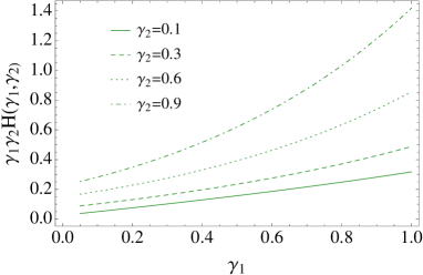
Eq. (42) can be re-written after taking the integrals over the angle and $p_{1,T}$ as

$\displaystyle H\left(\gamma_{1},\gamma_{2}\right)\,\,=\,\,\,\int^{1}_{0}dx\left(x^{2\gamma_{1}-1}\,+\,x^{2\gamma_{2}-1}\right)$ (43)
$\displaystyle\times\,\,\Bigg{(}(1-x)^{2(\gamma_{1}+\gamma_{2})}{}_{2}F_{1}\left(\frac{1}{2},-\gamma_{1}-\gamma_{2},1,-\frac{4x}{(1-x)^{2}}\right)\,+\,(1+x)^{2(\gamma_{1}+\gamma_{2})}{}_{2}F_{1}\left(\frac{1}{2},-\gamma_{1}-\gamma_{2},1,\frac{4x}{(1+x)^{2}}\right)\Bigg{)}$

We illustrate the behavior of this function in Fig. 4. Note, that $H\left(\gamma_{1},\gamma_{2}\right)$ is symmetric with respect to the change $\gamma_{1}\to\gamma_{2}$ ( $H\left(\gamma_{1},\gamma_{2}\right)=H\left(\gamma_{2},\gamma_{1}\right)$).

Refer to caption
Figure 4: The behavior of function $H\left(\gamma_{1},\gamma_{2}\right)$.

The particular solution to Eq. (40) has a simple form:

$$\Phi\left(\omega,\gamma_{1},\gamma_{2}\right)\,\,=\,\,\frac{H\left(\gamma_{1},\gamma_{2}\right)\,\phi\left(\omega,\gamma_{1}+\gamma_{2}\right)}{\omega\,-\,\bar{\alpha}_{S}\left(\chi\left(\gamma_{1}\right)\,+\,\chi\left(\gamma_{2}\right)\right)}\,=\,\frac{H\left(\gamma_{1},\gamma_{2}\right)\,\phi_{\rm in}\left(\gamma_{1}+\gamma_{2}\right)}{\left(\omega\,-\,\bar{\alpha}_{S}\left(\chi\left(\gamma_{1}\right)\,+\,\chi\left(\gamma_{2}\right)\right)\right)\,\left(\omega\,-\,\bar{\alpha}_{S}\chi\left(\gamma_{1}+\gamma_{2}\right)\right)}$$ (44)

where$\phi_{\rm in}$ can be found from the initial conditions for the single gluon density.

From Eq. (44) we obtain the particular solution for $\Phi\left(Y-y,p_{1,T};Y-y,p_{2,T};q_{T}\right)$

$\displaystyle\Phi_{\rm part}\left(Y-y,p_{1,T};Y-y,p_{2,T};q_{T}\right)\,\,=$ (45)
$\displaystyle\!\!\!\int^{\epsilon+i\infty}_{\epsilon-i\infty}\frac{d\gamma_{1}}{2\pi i}\int^{\epsilon+i\infty}_{\epsilon-i\infty}\frac{d\gamma_{2}}{2\pi i}\,e^{\gamma_{1}\xi_{1}\,+\,\gamma_{2}\xi_{2}}\frac{\bar{\alpha}_{S}^{2}\,H\left(\gamma_{1},\gamma_{2}\right)\,\phi_{\rm in}\left(\gamma_{1}+\gamma_{2}\right)}{\bar{\alpha}_{S}\left(\chi\left(\gamma_{1}\right)\,+\,\chi\left(\gamma_{2}\right)\,-\,\chi\left(\gamma_{1}+\gamma_{2}\right)\right)}\Bigg{\{}e^{\bar{\alpha}_{S}\left(\chi\left(\gamma_{1}\right)\,+\,\chi\left(\gamma_{2}\right)\right)\,\left(Y-y\right)}\,\,-\,\,e^{\bar{\alpha}_{S}\chi\left(\gamma_{1}+\gamma_{2}\right)\,\left(Y-y\right)}\Bigg{\}}$

where $\xi_{1}\,=\,\ln\left(p^{2}_{1,T}\right)$ and $\xi_{2}\,=\,\ln\left(p^{2}_{2,T}\right)$. The general solution will be a sum of the particular solution and the solution to the homogeneous equation, and it has the following form

$\displaystyle\Phi\left(Y-y,p_{1,T};Y-y,p_{2,T};q_{T}\right)\,\,=$ (46)
$\displaystyle\,\,\Phi_{\rm part}\left(Y-y,p_{1,T};Y-y,p_{2,T};q_{T}\right)\,+\,\!\!\!\int^{\epsilon+i\infty}_{\epsilon-i\infty}\frac{d\gamma_{1}}{2\pi i}\int^{\epsilon+i\infty}_{\epsilon-i\infty}\frac{d\gamma_{2}}{2\pi i}\,e^{\gamma_{1}\xi_{1}\,+\,\gamma_{2}\xi_{2}}\Phi_{\rm in}\left(\gamma_{1},\gamma_{2}\right)\,e^{\bar{\alpha}_{S}\left(\chi\left(\gamma_{1}\right)\,+\,\chi\left(\gamma_{2}\right)\right)\,\left(Y-y\right)}\,\,=$
$\displaystyle\,\,\int^{\epsilon+i\infty}_{\epsilon-i\infty}\frac{d\gamma_{1}}{2\pi i}\int^{\epsilon+i\infty}_{\epsilon-i\infty}\frac{d\gamma_{2}}{2\pi i}\,e^{\gamma_{1}\xi_{1}\,+\,\gamma_{2}\xi_{2}}\Bigg{\{}\Bigg{[}\frac{\bar{\alpha}_{S}H\left(\gamma_{1},\gamma_{2}\right)\,\phi_{\rm in}\left(\gamma_{1}+\gamma_{2}\right)}{\left(\chi\left(\gamma_{1}\right)\,+\,\chi\left(\gamma_{2}\right)\,-\,\chi\left(\gamma_{1}+\gamma_{2}\right)\right)}\,+\,\Phi_{\rm in}\left(\gamma_{1},\gamma_{2}\right)\Bigg{]}e^{\bar{\alpha}_{S}\left(\chi\left(\gamma_{1}\right)\,+\,\chi\left(\gamma_{2}\right)\right)\,\left(Y-y\right)}$
$\displaystyle\,\,-\,\,\frac{\bar{\alpha}_{S}H\left(\gamma_{1},\gamma_{2}\right)\,\phi_{\rm in}\left(\gamma_{1}+\gamma_{2}\right)}{\left(\chi\left(\gamma_{1}\right)\,+\,\chi\left(\gamma_{2}\right)\,-\,\chi\left(\gamma_{1}+\gamma_{2}\right)\right)}e^{\bar{\alpha}_{S}\chi\left(\gamma_{1}+\gamma_{2}\right)\,\left(Y-y\right)}\Bigg{\}}$

The integrals over $\gamma_{1}$ and $\gamma_{2}$ in the first term of Eq. (46) can be evaluated using the method of steepest descend with the saddle point for both $\gamma$’s close to $\frac{1}{2}$, where we can use the diffusion approximation (see Eq. (41)) for $\chi(\gamma)$. The values of $\gamma$’s at the saddle point are the following:

$$\gamma^{\rm SP}_{1}\,\,=\,\,\frac{1}{2}-\frac{\xi_{1}}{2\bar{\alpha}_{S}D\left(Y-y\right)};~{}~{}~{}~{}~{}\gamma^{\rm SP}_{2}\,\,=\,\,\frac{1}{2}-\frac{\xi_{2}}{2\bar{\alpha}_{S}D\left(Y-y\right)};$$ (47)

After integration over $\gamma_{1}$ and $\gamma_{2}$ in the vicinities of these saddle points we obtain the contribution:

$$\Phi\left(Y-y,p_{1,T};Y-y,p_{2,T};q_{T}\right)\,\,=\,\,\frac{1}{4\pi}\frac{1}{\bar{\alpha}_{S}D\left(Y-y\right)}\Bigg{[}\dots\Bigg{]}_{\gamma_{1}=\gamma^{\rm SP}_{1};\gamma_{2}=\gamma^{\rm SP}_{2}}\!\!\!\!\!\!\!\!\exp\left(2\bar{\alpha}_{S}\omega_{0}\left(Y-y\right)\,-\,\frac{\xi^{2}_{1}+\xi_{2}^{2}}{4\bar{\alpha}_{S}D\left(Y-y\right)}\right)$$ (48)

This contribution is proportional to $\phi\left(Y-y,\xi_{1}\right)\,\phi\left(Y-y,\xi_{2}\right)$ and in agreement with Eq. (1).

In the second term the integration over $\gamma_{1}+\gamma_{2}$ can be taken using the method of steepest descend, leading to

$$(\gamma_{1}+\gamma_{2})^{\rm SP}\,=\,\frac{1}{2}\,-\,\frac{\xi_{1}+\xi_{2}}{2\bar{\alpha}_{S}D\left(Y-y\right)}$$ (49)

This integration generates the contribution which is proportional to $\exp\left(\bar{\alpha}_{S}\omega_{0}\left(Y-y\right)\,-\,\left(\xi_{1}+\xi_{2}\right)^{2}/\left(4\bar{\alpha}_{S}D\left(Y-y\right)\right)\right)$. Comparing this contribution with Eq. (95), one can see that it is suppressed at large values of ( $Y-y$) .

IV The interference diagram in the BFKL evolution

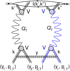
The interference diagram is shown in Fig. 5-a. In this diagram the $t$-channel gluons with the same color and with rapidities larger than $y^{\prime}$, are in colorless states. For rapidities, that are less than $y^{\prime}$, $t$ channel gluons with rapidities $y_{1}$ and with $y_{2}$ are in a colorless state. The arguments for such a color structure of this diagram stem from the first diagram with the exchange of two identical gluons, shown in Fig. 5-b. In this diagram all emitted gluons with rapidities larger than $y^{\prime}$, can be absorbed in the solution of the evolution equation without the Bose-Einstein enhancement, and can be used as a solution of Eq. (1). In this solution the double gluon density can be viewed as the exchange of two BFKL Pomerons, shown in Fig. 5-b.

Refer to caption Refer to caption Refer to caption
Fig. 5-a Fig. 5-b Fig. 5-c
Figure 5: The interference diagram.Fig. 5-a: For gluons with rapidities larger than $y^{\prime}$, the $t$-channel gluons, which are shown by the same color helical lines, are in a colorless state in the $t$-channel. The gluons with $y_{1}$ and with $y_{2}$ are in a colorless states as indicated by arrows in Fig. 1. The black circles denote the Lipatov vertex $\Gamma_{\mu}$. Fig. 5-b: This is the diagram of Fig. 1-a, which is re-drawn through the BFKL Pomerons denoted by wavy lines. Their colors in the figure indicate the gluons that constitute the pomerons (see Fig. 5-b). The gluons with $y_{1},p_{1,T}$ as well as gluons with $y_{2},p_{2,T}$ are in colorless states. $\boldsymbol{Q}^{\prime}_{T}\,=\,\boldsymbol{k}-\boldsymbol{p}_{2,T}$. $V$ denote the vertices of gluon-Pomeron interaction. Fig. 5-c: This diagram is the Born approximation of the diagram of Fig. 5-b in the case of an onium target. This diagram is in accord with Eq. (1).

These Pomerons carry transferred momenta $\boldsymbol{Q}^{\prime}_{T}$ and $-\boldsymbol{Q}^{\prime}_{T}$, respectively, where $\boldsymbol{Q}^{\prime}_{T}\,=\,\boldsymbol{k}\,-\,\boldsymbol{p}_{2,T}$. Therefore, we first need to deal with the BFKL Pomeron with non zero transfer momentum . However, before discussing this problem we calculate the diagram of Fig. 5-c, which is the diagram of Fig. 5-b in the Born approximation. Denoting the wave function of the colorless dipole ( the onium state of a heavy quark and antiquark) by $\Psi\left(q_{T},z\right)$, where $q_{T}$ is the transverse momentum of the quark and $z$ its fraction of the energy. We obtain that the component of the gluonic wave function with one emitted gluon with transverse momentum $p_{1,T}$ and rapidity $y_{1}$ is equal to MUDI ; KOLEB

$$\Psi^{(1)}\left(\boldsymbol{q}_{T},z;\boldsymbol{p}_{1,T},y_{1}\right)\,=\,g\lambda^{a}\frac{\boldsymbol{p}_{1,T}\cdot\boldsymbol{\epsilon}^{\lambda}_{1}}{p^{2}_{1,T}}\Bigg{(}\Psi\left(\boldsymbol{q}_{T},z\right)\,\,-\,\,\Psi\left(\boldsymbol{q}_{T}+\boldsymbol{p}_{1,T},z\right)\Bigg{)}$$ (50)

where $\lambda^{a}$ denotes the Gell-Mann matrix and $\boldsymbol{\epsilon}^{\lambda}$ is the polarization vector of the gluon with the helicity $\lambda$. The single gluon density has the form

$$\phi\left(y_{1},p_{1,T}\right)\,\,=\,\,\int^{1}_{0}\frac{dz}{z(1-z)}\int d^{2}q_{T}|\Psi^{(1)}\left(\boldsymbol{q}_{T},z;\boldsymbol{p}_{1,T},y_{1}\right)|^{2}\,\,=\,\,\frac{\alpha_{S}C_{F}}{\pi}\frac{1}{p^{2}_{1,T}}\,\left(G\left(0\right)-G\left(4p^{2}_{T}\right)\right)$$ (51)

In the integral over $z$, the lower limit is $e^{-Y+y}$, but we assumed that this integral is convergent and we can safely take this limit equal to zero.

$$G\left(\boldsymbol{p}_{T}\right)\,\,=\,\,\int\frac{dz}{z(1-z)}\int d^{2}re^{i\boldsymbol{p}_{T}\cdot\boldsymbol{r}}|\Psi\left(r,z\right)|^{2}~{}~{}~{}~{}~{}\mbox{where}~{}~{}~{}\int d^{2}r\int\frac{dz}{z(1-z)}|\Psi\left(r,z\right)|^{2}\,\,=\,\,1;$$ (52)

The emission of the second gluon with $y_{2}$ and $p_{2,T}$ leads to the wave function

$\displaystyle\Psi^{(1,1)}\left(\boldsymbol{q}_{T},z;\boldsymbol{p}_{1,T},y_{1};\boldsymbol{p}_{2,T},y_{2}\right)\,=$ (53)
$\displaystyle\,g^{2}\lambda^{a}\lambda^{b}\frac{\boldsymbol{p}_{1,T}\cdot\boldsymbol{\epsilon}^{\lambda}_{1}}{p^{2}_{1,T}}\frac{\boldsymbol{p}_{2,T}\cdot\boldsymbol{\epsilon}^{\lambda}_{2}}{p^{2}_{2,T}}\Bigg{(}\Psi\left(\boldsymbol{q}_{T},z\right)\,\,-\,\,\Psi\left(\boldsymbol{q}_{T}+\boldsymbol{p}_{1,T},z\right)\,\,-\,\,\Psi\left(\boldsymbol{q}_{T}+\boldsymbol{p}_{2,T},z\right)\,\,+\,\,\Psi\left(\boldsymbol{q}_{T}+\boldsymbol{p}_{1,T}+\boldsymbol{p}_{2,T},z\right)\Bigg{)}$

Using the expression for the Lipatov vertex $\Gamma_{\mu}$ which has the form BFKL ; KOLEB

$$\Gamma_{\mu}\left(k^{\prime},k\right)\,\,=\,\,2g\,f^{abc}\Bigg{(}k^{\prime}_{T,\mu}\,-\,\frac{k^{\prime 2}_{T}}{l^{2}_{T}}\,l_{T,\mu}\Bigg{)}$$ (54)

where $l_{\mu}\,=\,k^{\prime}_{T,\mu}\,-\,k_{T,\mu}$ is the momentum of the emitted gluon, as well as Eq. (53) we obtain for Fig. 5-c the following contribution

A(Fig.5c)\displaystyle A\left({Fig.~{}\ref{intdi}}-c\right)\,\, $\displaystyle\propto$ $\displaystyle\,\,\int d^{2}k_{T}\,I\left(\boldsymbol{p}_{2,T},\boldsymbol{k}_{T}\right)\frac{\left(\boldsymbol{k}_{T}\cdot\boldsymbol{p}_{2,T}\right)^{2}}{\left(p^{2}_{2,T}\,k^{2}_{T}\right)^{2}}\underbrace{\frac{k^{2}_{T}\,p^{2}_{1,T}}{\left(\boldsymbol{k}_{T}-\boldsymbol{p}_{1,T}\right)^{2}}}_{\Gamma_{\mu}\Gamma_{\mu}}\frac{1}{p^{4}_{1,T}}$ (55)
$\displaystyle\,\,=\,\,$ $\displaystyle\,\,\int d^{2}k_{T}\,I\left(\boldsymbol{p}_{2,T},\boldsymbol{k}_{T}\right)\frac{\left(\boldsymbol{k}_{T}\cdot\boldsymbol{p}_{2,T}\right)^{2}}{\left(p^{2}_{2,T}\,k^{2}_{T}\right)^{2}}\frac{k^{2}_{T}\,p^{2}_{1,T}}{\left(\boldsymbol{k}_{T}\,-\,\boldsymbol{p}_{2,T}-\Delta\boldsymbol{p}_{12,T}\right)^{2}}\frac{1}{p^{4}_{1,T}}\,$

where $\Delta\boldsymbol{p}_{12,T}\,=\boldsymbol{p}_{1,T}-\boldsymbol{p}_{2,T}$ and    $\left(\boldsymbol{p}_{2,T},\boldsymbol{k}_{T}\right)$ is equal to (see Ref.BEC5 )

$$I\left(\boldsymbol{p}_{2,T},\boldsymbol{k}_{T}\right)=2\,+\,G\left(2(\boldsymbol{k}_{T}+\boldsymbol{p}_{2,T})\right)+G\left(2(\boldsymbol{k}_{T}-\boldsymbol{p}_{2,T})\right)-G\left(2\boldsymbol{k}_{T}\right)-G\left(-2\boldsymbol{k}_{T}\right)\,-\,G\left(2\boldsymbol{p}_{2,T}\right)\,-\,G\left(-2\boldsymbol{p}_{2,T}\right);$$ (56)

In Eq. (53) for simplicity, we have omitted all color coefficients and coupling constants.

We see that the largest contribution stems from the region: $|\boldsymbol{p}_{2,T}-\boldsymbol{k}_{T}|\propto 1/r$, where $r$ is the size of the dipoles. Assuming that $p_{1,T}$ and $p_{2,T}$ are larger that $1/r$ this region leads to the contribution which is equal

A(Fig.5c)1p1,T2p2,T2d2kT(𝒌T𝒑2,TΔ𝒑12,T)2I(𝒑2,T,𝒌T)1p1,T2p2,T2πdq21|q2|Δ𝒑12,T|2|I(q)A\left({Fig.~{}\ref{intdi}}-c\right)\,\,\propto\,\,\frac{1}{p^{2}_{1,T}\,p^{2}_{2,T}}\int\frac{d^{2}k_{T}}{\left(\boldsymbol{k}_{T}\,-\,\boldsymbol{p}_{2,T}-\Delta\boldsymbol{p}_{12,T}\right)^{2}}\,I\left(\boldsymbol{p}_{2,T},\boldsymbol{k}_{T}\right)\,\sim\,\frac{1}{p^{2}_{1,T}\,p^{2}_{2,T}}\pi\int dq^{2}\frac{1}{|q^{2}-|\Delta\boldsymbol{p}_{12,T}|^{2}|}I(q) (57)

with $\boldsymbol{q}=\boldsymbol{k}_{T}-\boldsymbol{p}_{2,T}$. Eq. (57) generates $|q|\sim 1/r\,\ll\,p_{i,T}$ and shows that the Bose-Einstein enhancement is essential for $|\Delta\boldsymbol{p}_{12,T}|\,\ll\,p_{i,T}$ and the value of $|\Delta\boldsymbol{p}_{12,T}|$ is determined by the scale of the initial conditions for the double gluon density.

In other words we conclude that the first diagram leads to the double gluon density, which can be written in the form

$$\Phi^{\rm int}\,\propto\,\phi\left(y_{1},p_{1,T}\right)\,\phi\left(y_{2},p_{2,T}\right)\left\{\begin{array}[]{l}\,\propto\,\,{\rm Const}\,\,\,\,\,\mbox{for }\,\,\,|\Delta\boldsymbol{p}_{12,T}|\,r\,\,\leq\,1;\\ \\ \,\frac{1}{r^{2}\,|\Delta\boldsymbol{p}_{12,T}|^{2}}\,\,\,\,\,\mbox{for}\,\,\,|\Delta\boldsymbol{p}_{12,T}|\,r\,\,\geq\,1;\end{array}\right.\,\sim\,\,\frac{\phi\left(y_{1},p_{1,T}\right)\,\phi\left(y_{2},p_{2,T}\right)}{r^{2}\,|\Delta\boldsymbol{p}_{12,T}|^{2}\,\,+\,\,1}$$ (58)

In other words, the Bose-Einstein enhancement increases the double gluon densities for $\boldsymbol{p}_{1,T}\to\boldsymbol{p}_{2,T}$, as is expected and has been demonstrated in the correlation functionsBEC1 ; BEC2 ; BEC3 ; BEC4 ; BEC5 ; BEC6 .

Returning to the diagram of Fig. 5-b we see that generally the integration over $k_{T}$ enters the integration over momentum transfer of the BFKL Pomeron: $\boldsymbol{Q}^{\prime}_{T}\,=\,\boldsymbol{p}_{2,T}-\boldsymbol{k}_{T}$, and integration over $k_{T}$ that characterize the size of the dipole in the Pomeron vertices (see Fig. 5-b). The typical transverse momentum in the BFKL Pomeron vertices are about $p_{1,T}(p_{2,T})$ or about that of the saturation scale, at the rapidity of the vertex. On the other hand, the typical $Q^{\prime}_{T}\,\sim\,1/r$ where $r$ is the size of the largest dipole of the two interacting dipoles, which constitute the exchange of the BFKL Pomeron. For the diagrams of Fig. 5-b this largest dipole has a size of the hadron, whose double parton density we discuss.

The Green function of the BFKL Pomeron $G\left(\boldsymbol{r},\boldsymbol{R};\boldsymbol{Q}_{T};Y\right)$ is known in the mixed representation, where $r$ and $R$ are the sizes of two interacting dipoles, $Q_{T}$ denotes the momentum transferred by the Pomeron, and $Y$ the rapidity between the two dipoles. This Green function has the following formLIP ; NAPE :

$$G\left(\boldsymbol{r},\boldsymbol{R};\boldsymbol{Q}_{T};Y\right)\,=\,\,\frac{1}{16}\sum^{\infty}_{n=-\infty}\int^{\infty}_{-\infty}d\nu\frac{1}{\left(\nu^{2}+\frac{1}{4}(n-1)^{2}\right)\,\left(\nu^{2}+\frac{1}{4}(n+1)\right)}V_{\nu,n}\left(\boldsymbol{r},\boldsymbol{Q}_{T}\right)\,V^{*}_{\nu,n}\left(\boldsymbol{R},\boldsymbol{Q}_{T}\right)\,e^{\omega\left(\nu,n\right)\,Y}$$ (59)

where

$$\omega\left(\nu,n\right)\,\,=\,\,2\,\bar{\alpha}_{S}{\rm Re}\left(\psi\left(\frac{1}{2}+\frac{1}{2}|n|+\nu\right)-\psi\left(1\right)\right);~{}~{}~{}~{}~{}\mbox{and}~{}~{}~{}\omega\left(\nu,0\right)\,\,=\,\,\bar{\alpha}_{S}\chi\left(\frac{1}{2}+i\nu\right);$$ (60)

with $n=0,1,3\dots$ and $\chi\left(\gamma\right)$ from Eq. (41).

Each term in Eq. (59) has a very simple structure, being the typical contribution of a Regge pole exchange: the product of two vertices, which depend on the size of the dipole and $Q_{T}$, and the Regge-pole propagator $e^{\omega\left(\nu,n\right)\,Y}$. From Eq. (60) one can see that at large $Y$ the main contribution comes from the term with $n=0,$ and in what follows we will concentrate on this particular term.

The vertices with $n=0$ have been determined in Refs.LIP ; NAPE , and they have a simple form in the complex number representation for the point on the two dimensional plane: viz.

$$\mbox{For }\boldsymbol{r}(x,y):\,\,\rho=x+iy;\,\,\rho^{*}=x-iy;~{}~{}~{}~{}~{}\mbox{For }\boldsymbol{Q}_{T}(Q_{x},Q_{y}):\,\,q=Q_{x}+iQ_{y};\,\,q^{*}=Q_{x}-iQ_{y};$$ (61)

Using this notation the vertices have the following structure:

$$V_{\nu}\left(\boldsymbol{r},\boldsymbol{Q}_{T}\right)\,=\,r\,\left(Q^{2}_{T}\right)^{i\nu}\,\Gamma^{2}\left(1-i\nu\right)\Bigg{\{}J_{-i\nu}\left(\frac{1}{4}q^{*}\rho\right)\,J_{-i\nu}\left(\frac{1}{4}q\rho^{*}\right)\,\,-\,\,J_{i\nu}\left(\frac{1}{4}q^{*}\rho\right)\,J_{i\nu}\left(\frac{1}{4}q\rho^{*}\right)\Bigg{\}}$$ (62)

At $Q_{T}\to 0$ this vertex takes the form:

$$V_{\nu}\left(\boldsymbol{r},\boldsymbol{Q}_{T}\right)\,\xrightarrow{Q_{T}r\,\ll\,1}\,\,r\,\Bigg{\{}\left(\frac{r^{2}}{2^{6}}\right)^{-i\nu}\,-\,\left(Q^{2}\right)^{i\nu}\left(\frac{Q^{2}r^{2}}{2^{6}}\right)^{i\nu}\Bigg{\}}$$ (63)

Using that

$$J_{-i\nu}\left(z\right)\,\,\xrightarrow{z\,\gg\,1}\,\,\sin\left(\frac{1}{4}\pi+z+\frac{1}{2}i\pi\nu\right)\sqrt{\frac{2}{\pi}}\sqrt{\frac{1}{z}}$$ (64)

at $\nu\ll 1$ we obtain for $Q^{2}_{T}r^{2}\gg 1$

$$V_{\nu}\left(\boldsymbol{r},\boldsymbol{Q}_{T}\right)\,\,\xrightarrow{Q_{T}r\,\gg\,1}\,\,\left(Q^{2}_{T}\right)^{i\nu}\,\Gamma^{2}\left(1-i\nu\right)\,\,\cos\left(\frac{1}{2}\boldsymbol{Q}_{T}\cdot\boldsymbol{r}\right)\,\frac{4\,i\,\nu}{Q_{T}}$$ (65)

Returning to Eq. (59), one can see that the exchange of the BFKL Pomeron turns out to be small for $R\,Q_{T}\,>\,1$, where $R$ is the size of the larger of the two interacting dipoles. In the diagram of Fig. 5-b, the size of the smallest dipole is about $r\propto 1/p_{2,T}$, while $R$ is the dipole in the hadron which has a size of the order $1/\mu_{\rm soft}$, $\mu_{\rm soft}$ denotes the soft scale. In other words, we expect that $Q_{T}$ of the BFKL Pomerons is rather small, $Q_{T}\leq\,\mu_{\rm soft}$. Since $|\boldsymbol{Q}^{\prime}_{T}|\,=\,|\boldsymbol{k}_{T}-\boldsymbol{p}_{2,T}|\leq\mu_{\rm soft}\,\ll\,p_{2,T}$ we safely use for vertex $V_{\nu}\left(\boldsymbol{r},\boldsymbol{Q}_{T}\right)$ Eq. (63) which gives for the vertex in the momentum representation:

$$V_{\nu}\left(\boldsymbol{k}_{T},\boldsymbol{Q}_{T}\right)\,\,=\,\,r^{2}\,\int d^{2}re^{-i\boldsymbol{r}\cdot\boldsymbol{k}_{T}}\,V_{\nu}\left(\boldsymbol{r},\boldsymbol{Q}_{T}\right)$$ (66)

the following expression:

$$V_{\nu}\left(\boldsymbol{k}_{T},\boldsymbol{Q}_{T}\right)\,\,=\,\,2\pi\Bigg{(}\frac{\Gamma\left(\frac{1}{2}+i\nu\right)}{\Gamma\left(\frac{1}{2}-i\nu\right)}\left(2\,k^{2}_{T}\right)^{-\frac{1}{2}+i\nu}\,\,-\,\,\frac{\Gamma\left(\frac{1}{2}-i\nu\right)}{\Gamma\left(\frac{1}{2}+i\nu\right)}\left(Q^{2}_{T}\right)^{2i\nu}\left(2k^{2}_{T}\right)^{-\frac{1}{2}+i\nu}\Bigg{)}$$ (67)

Actually, the second term does not contribute to the scattering amplitude at small $Q_{T}$ (see Refs.LIP ; GOLELY ), and therefore the diagram of Fig. 5-b gives the following contribution:

$\displaystyle\frac{\partial\Phi^{\rm int}\left(Y-y,p_{1,T},p_{2,T}\right)}{\partial(Y-y)}\,$ $\displaystyle=$ $\displaystyle\,\frac{\bar{\alpha}_{S}}{N^{2}_{c}-1}\,\int^{-i\epsilon+\infty}_{-i\epsilon-\infty}\frac{d\nu_{1}}{2\pi}\int^{-i\epsilon+\infty}_{-i\epsilon-\infty}\frac{d\nu_{2}}{2\pi}e^{\bar{\alpha}_{S}\left(\chi\left(\nu_{1}\right)+\chi\left(\nu_{2}\right)\right)\left(Y-y\right)}$
$\displaystyle\times$ $\displaystyle\int\frac{d^{2}k^{\prime}_{T}d^{2}k^{\prime\prime}_{T}}{(2\pi)^{4}}\,I\left(\boldsymbol{k}^{\prime}_{T},\boldsymbol{k}^{\prime\prime}_{T}\right)V_{\nu_{1}}\left(\boldsymbol{k}^{\prime}_{T},\boldsymbol{Q}^{\prime}_{T}\right)\,V_{\nu_{2}}\left(\boldsymbol{k}^{\prime\prime}_{T},\boldsymbol{Q}^{\prime}_{T}\right)\,\int\frac{d^{2}Q^{\prime}_{T}}{\left(\Delta\boldsymbol{p}_{12,T}-\boldsymbol{Q}^{\prime}_{T}\right)^{2}}\left(2\,k^{2}_{T}\right)^{-1+i\nu_{1}+i\nu_{2}}$
$\displaystyle=$ $\displaystyle\,\frac{\bar{\alpha}_{S}}{N^{2}_{c}-1}\int\frac{d^{2}Q^{\prime}_{T}}{\left(\Delta\boldsymbol{p}_{12,T}-\boldsymbol{Q}^{\prime}_{T}\right)^{2}}\,\Phi_{2{I\!\!P}}\left(Y-y,p_{2,T},p_{2,T};Q^{\prime}_{T}\right)$ (69)

where $\Phi_{2{I\!\!P}}$ denotes the double gluon density due to exchange of two BFKL Pomerons. All other notations are shown in Fig. 5-b. The second line of the equation is written assuming that $\nu_{1}\,\ll\,1$ and $\nu_{2}\,\ll\,1$ at high energies, in accord with the diffusion approximation (see Eq. (41)). It is easy to see that this contribution is the Fourier transform of the emission term with $\rho^{(2)}$ in Eq. (II.2) in momentum representation. We need to add the gluon reggeization term to Eq. (IV) which is the Fourier transform of the second term with $\rho^{(2)}$ in Eq. (II.2). Therefore, we do not see any other contribution except the Bose-Einstein enhancement in the first diagrams. In the last line of the equation we consider $Q^{\prime}_{T}\,\ll\,p_{2T}$ and replace $k_{T}$ by $p_{2,T}$. From Eq. (69) one can see that the double parton density with $q_{T}=0$ (see Eq. (I)) can be obtained only if we know the double parton density for $q_{T}\neq 0$. For $q_{T}\neq 0$ the diagram of Fig. 5-b can be re-written in the form:

$$\frac{\partial\Phi^{\rm int}\left(Y-y,p_{1,T},p_{2,T};q_{T}\right)}{\partial(Y-y)}\,=\frac{\bar{\alpha}_{S}}{N^{2}_{c}-1}\int\frac{d^{2}Q^{\prime}_{T}}{\left(\Delta\boldsymbol{p}_{12,T}-\boldsymbol{Q}^{\prime}_{T}-\boldsymbol{q}_{T}\right)^{2}}\,\Phi_{2{I\!\!P}}\left(Y-y,p_{2,T},p_{2,T};\boldsymbol{Q}^{\prime}_{T}\right)$$ (70)

V BFKL evolution with Bose-Einstein enhancement

We need to change Eq. (38) by adding the interference diagram. To do this we have to change Eq. (IV), replacing $\Phi_{2{I\!\!P}}\left(Y-y,k_{T},p_{2,T};Q^{\prime}_{T}\right)$ by $\Phi\left(Y-y,k_{T},p_{2,T};Q^{\prime}_{T}\right)$ and taking into account the complete BFKL kernel of Eq. (19). Therefore, the contribution of the interference diagram to the evolution equation takes the form

$$\frac{\partial\Phi^{\rm int}\left(Y-y,p_{1,T},p_{2,T};q_{T}\right)}{\partial(Y-y)}\,=\,\int d^{2}k_{T}\,K\left(\boldsymbol{p}_{1T}-\boldsymbol{q}_{T},\boldsymbol{k}_{T};\boldsymbol{Q}^{\prime}_{T}\right)\Phi\left(Y-y,k_{T},p_{2,T};Q^{\prime}_{T}\right)$$ (71)

where $K$ denotes the kernel of Eq. (19). In Eq. (72) we have taken into account that $q_{T}\neq 0$. Substituting this kernel we reduce Eq. (72) to the form

$\displaystyle\frac{\partial\Phi^{\rm int}\left(Y-y,p_{1,T},p_{2,T};q_{T}\right)}{\partial(Y-y)}\,=$ (72)
$\displaystyle\,\frac{2\,\bar{\alpha}_{S}}{N^{2}_{c}-1}\Bigg{\{}\int d^{2}k_{T}\underbrace{\frac{1}{\left(\boldsymbol{k}_{T}-\boldsymbol{p}_{1,T}-q_{T}\right)^{2}}}_{\mbox{emission kernel}}\Phi\left(Y-y,k_{T},p_{2,T};Q^{\prime}_{T}\right)\,\,-\,\,\underbrace{\omega_{G}\left(\boldsymbol{p}_{2,T}-\boldsymbol{q}_{T}\right)}_{\mbox{reggeization kernel}}\,\Phi\left(Y-y,p_{2,T},p_{2,T};q_{T}\right)\Bigg{\}}$

As we have discussed in the previous section, the typical $Q^{\prime}_{T}$ is determined by the soft scale from the initial condition, as in Fig. 5-b, or by the saturation scale at rapidity $y^{\prime}>y$. Both are much smaller than $p_{iT}$, or the saturation momentum at rapidity $y$. Hence, we can neglect $\boldsymbol{Q}^{\prime}_{T}=\boldsymbol{k}_{T}-\boldsymbol{p}_{1T}$, as it is much smaller than $p_{i,T}$. Finally, Eq. (72) takes the form:

$\displaystyle\frac{\partial\Phi^{\rm int}\left(Y-y,p_{1,T},p_{2,T};q_{T}\right)}{\partial(Y-y)}\,\,=\,\,$ (73)
$\displaystyle\frac{\bar{\alpha}_{S}}{N^{2}_{c}-1}\int\frac{d^{2}Q^{\prime}_{T}}{\left(\Delta\boldsymbol{p}_{12,T}-\boldsymbol{Q}^{\prime}_{T}-\boldsymbol{q}_{T}\right)^{2}}\,\Big{\{}\Phi\left(Y-y,p_{2,T},p_{2,T};Q^{\prime}_{T}\right)\,-\,\omega_{G}\left(\boldsymbol{p}_{2,T}\right)\Phi\left(Y-y,p_{2,T},p_{2,T};q_{T}\right)\Big{\}}$

The second term in $\{\dots\}$ stems from the gluon reggeization, in which we neglect $q_{T}$ in comparison with $p_{i,T}$. Bearing Eq. (73) in mind, Eq. (38) takes the form:

$\displaystyle\frac{\partial\Phi\left(Y-y,p_{1,T};Y-y,p_{2,T};q_{T}\right)}{\partial\,\left(Y-y\right)}\,\,=\,\,\bar{\alpha}_{S}\int\frac{d^{2}k_{T}}{2\pi}\Bigg{\{}K\left(p_{1,T},k_{T};q_{T}\right)\,\Phi\left(Y-y,k_{T};Y-y,p_{2,T};q_{T}\right)\,+\,\,\Big{(}1\,\leftrightarrow\,2\Big{)}\Bigg{\}}\,$
$\displaystyle+\,\frac{\bar{\alpha}_{S}}{N^{2}_{c}-1}\Bigg{\{}\int\frac{d^{2}Q^{\prime}_{T}}{2\pi}\frac{1}{\left(\Delta\boldsymbol{p}_{12,T}-\boldsymbol{Q}^{\prime}_{T}-\boldsymbol{q}_{T}\right)^{2}}\,\Phi\left(Y-y,p_{1,T};Y-y,p_{1,T};Q^{\prime}_{T}\right)\,\,-\,\omega_{G}\left(\boldsymbol{p}_{2,T}\right)\Phi\left(Y-y,p_{2,T},p_{2,T};q_{T}\right)$
$\displaystyle\hskip 42.67912pt\,\,+\,\,\Big{(}1\,\leftrightarrow\,2\Big{)}\Bigg{\}}\,\,\,+\,\,\,\bar{\alpha}_{S}^{2}\,V\left(\boldsymbol{p}_{1,T},\boldsymbol{p}_{2,T},\boldsymbol{q}_{T}\right)\,\,\phi\left(Y-y^{\prime},\boldsymbol{p}_{1,T}+\boldsymbol{p}_{2,T}\right)$ (74)

We simplify the equation by first neglecting the $q_{T}$ dependence of the BFKL kernel in the first two terms of the R.H.S. of the equation, since as has been discussed, $q_{T}\,\ll\,k_{T}(p_{i,T})$. As the second step we go to the impact parameter representation:

$$\Phi\left(Y-y,p_{1,T};Y-y,p_{2,T};q_{T}\right)\,\,=\,\,\int d^{2}b\,e^{i\,\boldsymbol{q}_{T}\,\cdot\,\boldsymbol{b}}\Phi\left(Y-y,p_{1,T};Y-y,p_{2,T};b\right)$$ (75)

Eq. (V) then has the form:

$\displaystyle\frac{\partial\Phi\left(Y-y,p_{1,T};Y-y,p_{2,T};b\right)}{\partial\,\left(Y-y\right)}\,\,=$ (76)
$\displaystyle\bar{\alpha}_{S}\int\frac{d^{2}k_{T}}{2\pi}\Bigg{\{}K\left(p_{1,T},k_{T}\right)\,\Phi\left(Y-y,k_{T};Y-y,p_{2,T};b\right)\,+\,K\left(p_{2,T},k_{T}\right)\,\Phi\left(Y-y,p_{1,T};Y-y,k_{T};b\right)\Bigg{\}}\,$
$\displaystyle+\,\frac{\bar{\alpha}_{S}}{N^{2}_{c}-1}\Bigg{\{}\Bigg{(}S\left(b\,p_{1,T}\right)e^{i\,\boldsymbol{b}\,\cdot\,\Delta\boldsymbol{p}_{12,T}}\,-\,S\left(0\right)\Bigg{)}\Phi\left(Y-y,p_{1,T};Y-y,p_{1,T};b\right)\,\,\,\,\,+\,\,\,\,\,\Big{(}1\,\leftrightarrow\,2\Big{)}\Bigg{\}}$
$\displaystyle\,+\,\,\bar{\alpha}_{S}^{2}\,V\left(\boldsymbol{p}_{1,T},\boldsymbol{p}_{2,T},b\right)\,\,\phi\left(Y-y^{\prime},\boldsymbol{p}_{1,T}+\boldsymbol{p}_{2,T}\right)$

We need to re-write the kernel $1\Big{/}\left(\Delta\boldsymbol{p}_{12,T}-\boldsymbol{Q}^{\prime}_{T}-\boldsymbol{q}_{T}\right)^{2}$ to regularize the infrared singularity and to take into account that $|\boldsymbol{Q}^{\prime}_{T}|\,\ll\,p_{i,T}$. The last constraint was used in deriving the equation. We now replace the kernel by the expression

$$\frac{1}{\left(\Delta\boldsymbol{p}_{12,T}-\boldsymbol{Q}^{\prime}_{T}-\boldsymbol{q}_{T}\right)^{2}}\,\,\to\,\,\frac{1}{\left(\Delta\boldsymbol{p}_{12,T}-\boldsymbol{Q}^{\prime}_{T}-\boldsymbol{q}_{T}\right)^{2}+\mu^{2}}\,\,-\,\,\frac{1}{\left(\Delta\boldsymbol{p}_{12,T}-\boldsymbol{Q}^{\prime}_{T}-\boldsymbol{q}_{T}\right)^{2}+p^{2}_{1,T}}$$ (77)

One can see that the term with $\mu^{2}$ regularizes the infrared divergency, and the second term guarantees that only $Q^{\prime}_{T}$ and $q_{T}$ less than $p_{1,T}$, contribute to the integral. Calculating the Fourier transform of Eq. (77) we obtain

$$S\left(b\,p_{1,T}\right)\,\,=\,\,K_{0}\left(\mu\,b\right)\,-\,K_{0}\left(p_{1,T}\,b\right)$$ (78)

Since at $b\to 0$ $\left(b\,p_{1,T}\right)\,\to\ln\left(p^{2}_{1,T}/\mu^{2}\right)$, the reggeization term with $\omega_{G}\left(p_{1,t}\right)=\ln\left(p^{2}_{T}/\mu^{2}\right)$ cancels the infrared divergency in the difference $\Bigg{(}S\left(b\,p_{1,T}\right)e^{i\,\boldsymbol{b}\,\cdot\,\Delta\boldsymbol{p}_{12,T}}\,-\,S\left(0\right)\Bigg{)}$.

We first find the solution to the homogeneous equation re-writing it in the Mellin transform of Eq. (39). It has the form:

$\displaystyle\omega\,\Phi\left(\omega,\gamma_{1},\gamma_{2};b\right)\,\,=$ (79)
$\displaystyle\,\,\bar{\alpha}_{S}\,\left(\chi\left(\gamma_{1}\right)\,+\,\chi\left(\gamma_{2}\right)\right)\,\Phi\left(\omega,\gamma_{1},\gamma_{2};b\right)\,\,\,\,\,+\,\,\delta\Bigg{\{}\int^{\epsilon+i\infty}_{\epsilon-i\infty}\frac{d\gamma^{\prime}_{1}}{2\pi i}K\,\left(\gamma_{2},\gamma_{1}-\gamma^{\prime}_{1};b\right)\int^{\epsilon+i\infty}_{\epsilon-i\infty}\frac{d\gamma^{\prime}}{2\pi i}\Phi\left(\omega,\gamma^{\prime},\gamma^{\prime}_{1}-\gamma^{\prime};b\right)\,\,$
$\displaystyle+\,\,\int^{\epsilon+i\infty}_{\epsilon-i\infty}\frac{d\gamma^{\prime}_{1}}{2\pi i}K\,\left(\gamma_{1},\gamma_{2}-\gamma^{\prime}_{2};b\right)\int^{\epsilon+i\infty}_{\epsilon-i\infty}\frac{d\gamma^{\prime}}{2\pi i}\Phi\left(\omega,\gamma^{\prime},\gamma^{\prime}_{2}-\gamma^{\prime};b\right)\Bigg{\}}$

where $\delta=\bar{\alpha}_{S}/(N^{2}_{c}-1)$. $K\,\left(\gamma_{2},\gamma_{1}-\gamma^{\prime}_{1};b\right)$ is equal to

$\displaystyle K\left(\gamma_{2},\gamma_{1}-\gamma^{\prime}_{1};b\right)\,\,$ $\displaystyle=$ $\displaystyle\,\,\tilde{K}\left(\gamma_{2},\gamma_{1}-\gamma^{\prime}_{1};b\right)\,-\,\hat{K}\left(\gamma_{2},\gamma_{1}-\gamma^{\prime}_{1}\right);$ (80)
$\displaystyle\tilde{K}\left(\gamma_{2},\gamma_{1}-\gamma^{\prime}_{1};b\right)\,\,$ $\displaystyle=$ $\displaystyle\,\,\int p_{1,T}\,dp_{1,T}\,p_{2,T}\,dp_{2,T}\left(p^{2}_{1,T}\right)^{-\gamma_{1}}\left(p^{2}_{2,T}\right)^{-\gamma_{2}}J_{0}\left(b\,p_{1,T}\right)\,J_{0}\left(b\,p_{2,T}\right)\,S\left(b\,p_{1,T}\right)\,\left(p^{2}_{1,T}\right)^{\gamma^{\prime}_{1}-1}$
$\displaystyle\hat{K}\left(\gamma_{2},\gamma_{1}-\gamma^{\prime}_{1}\right)\,\,$ $\displaystyle=$ $\displaystyle\,\,\int p_{1,T}\,dp_{1,T}\,p_{2,T}\,dp_{2,T}\left(p^{2}_{1,T}\right)^{-\gamma_{1}}\left(p^{2}_{2,T}\right)^{-\gamma_{2}}\,\omega_{G}\left(p_{1,T}\right)\,\left(p^{2}_{1,T}\right)^{\gamma^{\prime}_{1}-1}$

For $K\left(\gamma_{2},\gamma_{1}-\gamma^{\prime}_{1};b=0\right)$ we have

$$K\left(\gamma_{2},\gamma_{1}-\gamma^{\prime}_{1};b=0\right)\,\,=\,\,-\,\frac{1}{4}\frac{1}{1-\gamma_{2}}\,\frac{1}{\left(\gamma^{\prime}_{1}-\gamma_{1}\right)^{2}}$$ (81)

Integrating over $\gamma^{\prime}_{1}$($\gamma^{\prime}_{2}$) we get the following equation

$\displaystyle\omega\,\Phi\left(\omega,\gamma_{1},\gamma_{2};b\right)\,\,=\,\,\bar{\alpha}_{S}\,\left(\chi\left(\gamma_{1}\right)\,+\,\chi\left(\gamma_{2}\right)\right)\,\Phi\left(\omega,\gamma_{1},\gamma_{2};b\right)\,\,$
$\displaystyle\,\,\,-\,\,\frac{\delta}{4}\Bigg{\{}\frac{1}{1-\gamma_{2}}\int^{\epsilon+i\infty}_{\epsilon-i\infty}\frac{d\gamma^{\prime}}{2\pi i}\Phi^{\prime}_{\gamma_{1}}\left(\omega,\gamma^{\prime},\gamma_{1}-\gamma^{\prime};b\right)\,\,+\,\,\frac{1}{1-\gamma_{1}}\int^{\epsilon+i\infty}_{\epsilon-i\infty}\frac{d\gamma^{\prime}}{2\pi i}\Phi^{\prime}_{\gamma_{2}}\left(\omega,\gamma^{\prime},\gamma_{2}-\gamma^{\prime};b\right)\Bigg{\}}$

We solve this equation using the iteration procedure with respect to the small parameter $\delta$, assuming that the solution without the interference term is equal to

$$\Phi^{(0)}\left(\omega,\gamma_{1},\gamma_{2}\right)\,\,=\,\,\frac{1}{\omega\,-\,\bar{\alpha}_{S}\left(\chi\left(\gamma_{1}\right)+\chi\left(\gamma_{2}\right)\right)}$$ (82)

Plugging this solution in Eq. (79), we obtain the following equation for the spectrum of the homogeneous equation:

$$1\,\,=\,\,-\,\frac{\delta}{4}\,\Bigg{\{}\frac{1}{1-\gamma_{2}}\int^{\epsilon+i\infty}_{\epsilon-i\infty}\frac{d\gamma^{\prime}}{2\pi i}\Phi^{(0)^{\prime}}_{\gamma_{1}}\left(\omega,\gamma^{\prime},\gamma_{1}-\gamma^{\prime}\right)\,\,+\,\,\frac{1}{1-\gamma_{1}}\int^{\epsilon+i\infty}_{\epsilon-i\infty}\frac{d\gamma^{\prime}}{2\pi i}\Phi^{(0)^{\prime}}_{\gamma_{2}}\left(\omega,\gamma^{\prime},\gamma_{2}-\gamma^{\prime}\right)\Bigg{\}}$$ (83)

In general for the BFKL kernel (see Eq. (19)) we cannot integrate the integral analytically. Instead, we use the diffusion approximation to obtain the analytical result:

$\displaystyle\int^{\epsilon+i\infty}_{\epsilon-i\infty}\frac{d\gamma^{\prime}}{2\pi i}\Phi^{(0)}\left(\omega,\gamma^{\prime},\gamma-\gamma^{\prime}\right)\,\,$ $\displaystyle=$ $\displaystyle\,\,\int^{\epsilon+i\infty}_{\epsilon-i\infty}\frac{d\gamma^{\prime}}{2\pi i}\frac{1}{\omega-\bar{\alpha}_{S}\underbrace{\left(2\omega_{0}+D\left(\left(\gamma^{\prime}-\frac{1}{2}\right)^{2}+\left(\gamma-\gamma^{\prime}-\frac{1}{2}\right)^{2}\right)\right)}_{\mbox{diffusion approximation}}}$
$\displaystyle=$ $\displaystyle\frac{1}{2}\frac{1}{\sqrt{2\bar{\alpha}_{S}D\left(\omega\,-\,2\bar{\alpha}_{S}\left(\omega_{0}+D\left(\frac{\gamma}{2}-\frac{1}{2}\right)^{2}\right)\right)}}\,=\,\frac{1}{2}\frac{1}{\sqrt{2\bar{\alpha}_{S}D\left(\omega\,-\,2\bar{\alpha}_{S}\chi_{\rm diff.~{}app.}\left(\frac{1}{2}\gamma\right)\right)}}$

where $\chi_{\rm diff.~{}app.}$ is the BFKL kernel in the diffusion approximation of Eq. (41).

Plugging Eq. (V) into Eq. (83), we reduce this equation to the form for $\gamma_{1}=\gamma_{2}$

$$1\,\,=\,\,\,\frac{\delta}{4\sqrt{2}}\sqrt{\bar{\alpha}_{S}D}\frac{1}{\left(\omega\,-\,2\bar{\alpha}_{S}\left(\omega_{0}+D\left(\frac{\gamma}{2}-\frac{1}{2}\right)^{2}\right)\right)^{3/2}}$$ (85)

Searching for the solution with the new intercept $\omega-2\bar{\alpha}_{S}\omega_{0}=\omega^{(1)}\left(\gamma_{1},\gamma_{2}\right)$, we obtain the solution for $\gamma_{1}=\gamma_{2}\to 1$.

$$\omega^{(1)}\left(\gamma_{1},\gamma_{2}\right)\,\,=\,\left(\frac{\delta}{4\sqrt{2}}\sqrt{\bar{\alpha}_{S}D}\right)^{2/3}\,\,=\,\,\frac{\bar{\alpha}_{S}}{\left(N^{2}_{c}-1\right)^{2/3}}\,\left(\frac{D}{32}\right)^{1/3}\,\,\approx\,\,0.8\,\frac{\bar{\alpha}_{S}}{\left(N^{2}-1\right)^{2/3}}\,=\,0.2\,\bar{\alpha}_{S}~{}~{}\mbox{for}N_{c}=3$$ (86)

Therefore, we see that the value of the intercept for the double parton density ($Y-y$) dependence, is larger than that for the product of single parton densities (see Eq. (1)), which is equal to

$$\Phi\left(Y-y,p_{1,T};Y-y,p_{2,T};q_{T}\right)\,\propto\,e^{\Delta_{2}\left(Y-y\right)};~{}~{}~{}~{}~{}\mbox{with}~{}~{}~{}\Delta_{2}\,=\,2\bar{\alpha}_{S}\omega_{0}\,\,+\,\,\frac{\bar{\alpha}_{S}}{\left(N^{2}_{c}-1\right)^{2/3}}\,\left(\frac{D}{32}\right)^{1/3}$$ (87)

Therefore, the difference $\Delta_{2}-2\bar{\alpha}_{S}\omega_{0}$ turns out to be proportional to $1/\left(N^{2}_{c}-1\right)^{2/3}$, which is a small number at large $N_{c}$. However, for $N_{c}=3$ (see Eq. (87)) $\Delta_{2}-2\bar{\alpha}_{S}\omega_{0}\approx 0.2\,\bar{\alpha}_{S}\approx 0.07\bar{\alpha}_{S}\omega_{0}$. This value of the correction leads to an effect of the order of 1 at $Y\approx 20$.

We can calculate the corrections of the order of $\delta^{2}$ to the intercept, using for the iteration $\Phi^{(1)}\left(\omega,\gamma_{1},\gamma_{2}\right)$ the form

$$\Phi^{(1)}\left(\omega,\gamma_{1},\gamma_{2}\right)\,\,=\,\,\frac{1}{\omega\,-\,2\omega_{0}\,-\,D\left(\left(\gamma_{1}-\frac{1}{2}\right)^{2}+\left(\gamma_{2}-\frac{1}{2}\right)^{2}\right)\,\,-\,\,\omega^{(1)}\left(\gamma_{1},\gamma_{2}\right)}$$ (88)

However, we expect negligible values for this correction, and we proceed to find the solution of Eq. (V) using Eq. (88), as the solution for the homogeneous equation.

VI High energy behaviour of the double gluon densities

Using the result of Eq. (88) we can write Eq. (40) in the following form:

$$\omega\,\Phi\left(\omega,\gamma_{1},\gamma_{2}\right)\,\,=\,\,\bar{\alpha}_{S}\,\left(\chi\left(\gamma_{1}\right)\,+\,\chi\left(\gamma_{2}\right)\,\,+\,\,\omega^{(1)}\left(\gamma_{1},\gamma_{2}\right)\right)\,\Phi\left(\omega,\gamma_{1},\gamma_{2}\right)\,\,+\,\,H\left(\gamma_{1},\gamma_{2}\right)\phi\left(\gamma_{1}+\gamma_{2}\right)$$ (89)

Eq. (89) generates the following particular solution, which is a direct generalization of Eq. (45):

$\displaystyle\Phi_{\rm part}\left(Y-y,p_{1,T};Y-y,p_{2,T};q_{T}\right)\,\,=\,\,\int^{\epsilon+i\infty}_{\epsilon-i\infty}\frac{d\gamma_{1}}{2\pi i}\int^{\epsilon+i\infty}_{\epsilon-i\infty}\frac{d\gamma_{2}}{2\pi i}$ (90)
$\displaystyle\,e^{\gamma_{1}\xi_{1}\,+\,\gamma_{2}\xi_{2}}\frac{\bar{\alpha}_{S}\,H\left(\gamma_{1},\gamma_{2}\right)\,\phi_{\rm in}\left(\gamma_{1}+\gamma_{2}\right)}{\omega\left(\gamma_{1}\right)\,+\,\omega\left(\gamma_{2}\right)\,+\,\omega^{(1)}\left(\gamma_{1},\gamma_{2}\right)\,-\,\omega\left(\gamma_{1}+\gamma_{2}\right)}\Bigg{\{}e^{\left(\omega\left(\gamma_{1}\right)\,+\,\omega\left(\gamma_{2}\right)\,\,+\,\,\omega^{(1)}\left(\gamma_{1},\gamma_{2}\right)\right)\,\left(Y-y\right)}\,\,-\,\,e^{\bar{\alpha}_{S}\chi\left(\gamma_{1}+\gamma_{2}\right)\,\left(Y-y\right)}\Bigg{\}}$

The general solution can be written in the same form as Eq. (46) leading to the following expression

$\displaystyle\Phi\left(Y-y,p_{1,T};Y-y,p_{2,T};q_{T}\right)\,\,=\,\,\,\int^{\epsilon+i\infty}_{\epsilon-i\infty}\frac{d\gamma_{1}}{2\pi i}\int^{\epsilon+i\infty}_{\epsilon-i\infty}\frac{d\gamma_{2}}{2\pi i}\,e^{\gamma_{1}\xi_{1}\,+\,\gamma_{2}\xi_{2}}$ (91)
$\displaystyle\Bigg{\{}\Bigg{[}\frac{\bar{\alpha}_{S}^{2}H\left(\gamma_{1},\gamma_{2}\right)\,\phi_{\rm in}\left(\gamma_{1}+\gamma_{2}\right)}{\left(\omega\left(\gamma_{1}\right)\,+\,\omega\left(\gamma_{2}\right)\,+\omega^{(1)}\left(\gamma_{1},\gamma_{2}\right)\,-\,\omega\left(\gamma_{1}+\gamma_{2}\right)\right)}\,+\,\Phi_{\rm in}\left(\gamma_{1},\gamma_{2}\right)\Bigg{]}e^{\left(\omega\left(\gamma_{1}\right)\,+\,\omega\left(\gamma_{2}\right)\,+\,\omega^{(1)}\left(\gamma_{1},\gamma_{2}\right)\right)\,\left(Y-y\right)}$
$\displaystyle\,\,-\,\,\frac{\bar{\alpha}_{S}^{2}H\left(\gamma_{1},\gamma_{2}\right)\,\phi_{\rm in}\left(\gamma_{1}+\gamma_{2}\right)}{\left(\omega\left(\gamma_{1}\right)\,+\,\omega\left(\gamma_{2}\right)\,+\omega^{(1)}\left(\gamma_{1},\gamma_{2}\right)\,-\,\omega\left(\gamma_{1}+\gamma_{2}\right)\right)}e^{\bar{\alpha}_{S}\chi\left(\gamma_{1}+\gamma_{2}\right)\,\left(Y-y\right)}\Bigg{\}}$

As have been discussed previously, we can use the method of steepest descend to evaluate the integrals over $\gamma_{1}$ and $\gamma_{2}$ in the first term of Eq. (91). To do this we need to know the dependence of $\omega^{(1)}\left(\gamma_{1},\gamma_{2}\right)$ in $\gamma_{1}$ and $\gamma_{2}$. Solving Eq. (85) we see that

$$\omega^{(1)}\left(\gamma,\gamma\right)\,\,=\,\,\omega^{(1)}_{0}\,-\,\,\frac{3}{2}\,\bar{\alpha}_{S}\,D\,\gamma\,\left(\gamma-\frac{2}{3}\right)$$ (92)

where $\omega^{(1)}_{0}$ is given by Eq. (87).

The values of the saddle point turn out to be close to $\frac{1}{2}$ for both $\gamma$’s. In the vicinity $\gamma_{1}\to\frac{1}{2}$ and $\gamma_{2}\to\frac{1}{2}$ we have the following expansion

$$\omega\left(\gamma_{1}\right)\,+\,\omega\left(\gamma_{2}\right)\,+\,\omega^{(1)}\left(\gamma_{1},\gamma_{2}\right)\,\,=\,\,2\bar{\alpha}_{S}\omega_{0}\,+\,\omega^{(1)}_{0}\,+\,\frac{\bar{\alpha}_{S}\,D}{4}\,\left(\left(1-\gamma_{1}\right)^{2}+\left(1-\gamma_{2}\right)^{2}\right)$$ (93)

From Eq. (93) we obtain that the values of $\gamma$’s at the saddle point are the following:

$$\gamma^{\rm SP}_{1}\,\,=\,\,1-\frac{2\,\xi_{1}}{\bar{\alpha}_{S}\,D\,\left(Y-y\right)};~{}~{}~{}~{}~{}~{}~{}\gamma^{\rm SP}_{2}\,\,=\,\,1-\frac{2\,\xi_{2}}{\bar{\alpha}_{S}D\left(Y-y\right)};$$ (94)

After integration over $\gamma_{1}$ and $\gamma_{2}$ in vicinities of these saddle points we obtain the contribution:

$\displaystyle\Phi\left(Y-y,p_{1,T};Y-y,p_{2,T};q_{T}\right)\,\,=$ (95)
$\displaystyle\,\,\frac{1}{4\pi}\frac{2}{\bar{\alpha}_{S}D\left(Y-y\right)}\Bigg{[}\dots\Bigg{]}_{\gamma_{1}=\gamma^{\rm SP}_{1};\gamma_{2}=\gamma^{\rm SP}_{2}}\!\!\!\!\!\!\!\!\exp\left(2\bar{\alpha}_{S}\,\Delta_{2}\left(Y-y\right)\,\,-\,2\,\frac{\xi^{2}_{1}+\xi_{2}^{2}}{\bar{\alpha}_{S}D\left(Y-y\right)}\right)$

One can see that this contribution is not proportional to $\phi\left(Y-y,\xi_{1}\right)\,\phi\left(Y-y,\xi_{2}\right)$, and contradicts Eq. (1). It should be stressed that Eq. (1) violates both the $Y-y$ dependence due to the intercept $\Delta_{2}\,>\,2\bar{\alpha}_{S}\omega_{0}$, and the $\xi_{1}$($\xi_{2}$) dependence (compare this equation with Eq. (95)). Note that the change in the $\xi$ shape of the distribution, has no suppression of $1/\left(N^{2}_{c}-1\right)$.

VII Conclusions

In this paper we found that in the BFKL evolution, the Bose-Einstein enhancement leads to a faster increase of the double parton densities than the product of two single parton distributions. This effect has been discussed by us for the DGLAP evolution in the region of low $x$GOLELAST . On the qualitative level, the DGLAP and BFKL evolution lead to large correlations at high energies, due to the correlations of the identical gluons. It should be noted that all $1/(N^{2}_{c}-1)$ corrections in the double gluon densities stem from the Bose-Einstein enhancement.

The BFKL evolution generates the power dependence on $x$ ( $\Phi\propto\left(1/x\right)^{\Delta_{2}}$ with $\Delta_{2}-2\omega_{0}>0$, where $\omega_{0}$ is the intercept of the BFKL Pomeron, this difference turns out to be numerically small, since it is proportional to $\bar{\alpha}_{S}/\left(N^{2}_{c}-1\right)^{2/3}$.

In particular, these correlations clarify the physical meaning of the increase of the anomalous dimension of the twist four operator that has been discussed in Refs. BART1 ; BART2 ; LET2 ; LLS ; LALE ; BARY . It should be stressed that we obtain the intercept for the double gluon density is proportion; to $1/\left(N^{2}_{c}-1\right)^{2/3}$ which is quite different from the twist four intercept, which is proportional to $1/\left(N^{2}_{c}-1\right)^{2}$. However, in the case of the anomalous dimensions, corrections other than the Bose-Einstein enhancement, of the order of $1/(N^{2}_{c}-1)$, contribute so making the calculation of the energy behavior of the twist four operator to be a different problem.

We view this paper as the next step in understanding the role of the identical parton correlations in the parton evolution. The next project that we plan to consider, is to include the identical parton correlations in the DGLAP evolution at finite $x$. We believe that the most interesting question in his part of the program is to include the Pauli blocking for quarks and antiquarks (see Ref.ALAM ).

VIII Acknowledgements

We thank our colleagues at Tel Aviv university and UTFSM for encouraging discussions. Our special thanks go to Alex Kovner and Misha Lublinsky for elucidating discussions on the role of the Bose - Einstein correlation in the CGC effective theory.

This research was supported by the BSF grant 2012124, by Proyecto Basal FB 0821(Chile), Fondecyt (Chile) grant 1180118 and by CONICYT grant PIA ACT1406.

References

  • (1) V. Shelest, A. Snigirev and G. Zinovev, Phys.Lett. B113, 325 (1982).
  • (2) G. Zinovev, A. Snigirev and V. Shelest, Theor.Math.Phys. 51, 523 (1982).
  • (3) A. M. Snigirev, Phys. Rev. D68, 114012 (2003), [hep-ph/0304172].
  • (4) V. L. Korotkikh and A. M. Snigirev, Phys. Lett. B594, 171 (2004), [hep-ph/0404155].
  • (5) J. R. Gaunt and W. J. Stirling, JHEP 03, 005 (2010), [0910.4347].
  • (6) B. Blok, Y. Dokshitzer, L. Frankfurt and M. Strikman, Phys.Rev. D83, 071501 (2011), [1009.2714].
  • (7) R. K. Ellis, W. Furmanski and R. Petronzio, Nucl.Phys. B212, 29 (1983).
  • (8) A. Bukhvostov, G. Frolov, L. Lipatov and E. Kuraev, Nucl.Phys. B258, 601 (1985).
  • (9) E. Laenen, E. Levin and A. G. Shuvaev, Nucl. Phys. B 419, 39 (1994), [hep-ph/9308294].
  • (10) E. Laenen and E. Levin, Nucl. Phys. B 451, 207 (1995), [hep-ph/9503381].
  • (11) F. A. Ceccopieri, Phys. Lett. B697, 482 (2011), [1011.6586].
  • (12) M. Diehl and A. Schafer, Phys. Lett. B698, 389 (2011), [1102.3081].
  • (13) J. R. Gaunt and W. J. Stirling, JHEP 1106, 048 (2011), [1103.1888].
  • (14) M. Ryskin and A. Snigirev, Phys.Rev. D83, 114047 (2011), [1103.3495].
  • (15) J. Bartels and M. G. Ryskin, “Recombination within Multi-Chain Contributions in pp Scattering,” arXiv:1105.1638 [hep-ph].
  • (16) B. Blok, Y. Dokshitzer, L. Frankfurt and M. Strikman, Eur.Phys.J. C72, 1963 (2012), [1106.5533].
  • (17) M. Diehl, D. Ostermeier and A. Schafer, JHEP 1203, 089 (2012), [1111.0910].
  • (18) M. Luszczak, R. Maciula and A. Szczurek, Phys. Rev. D85, 094034 (2012), [1111.3255].
  • (19) A. V. Manohar and W. J. Waalewijn, Phys.Rev. D85, 114009 (2012), [1202.3794].
  • (20) M. Ryskin and A. Snigirev, Phys.Rev. D86, 014018 (2012), [1203.2330].
  • (21) J. R. Gaunt, JHEP 1301, 042 (2013), [1207.0480].
  • (22) B. Blok, Y. Dokshitzer, L. Frankfurt and M. Strikman, Eur.Phys.J. C74, 2926 (2014), [1306.3763].
  • (23) A. van Hameren, R. Maciula and A. Szczurek, Phys. Rev. D89, 094019 (2014), [1402.6972].
  • (24) R. Maciula and A. Szczurek, Phys. Rev. D90, 014022 (2014), [1403.2595].
  • (25) A. Snigirev, N. Snigireva and G. Zinovjev, Phys.Rev. D90, 014015 (2014), [1403.6947].
  • (26) K. Golec-Biernat and E. Lewandowska, Phys.Rev. D90, 094032 (2014), [1407.4038].
  • (27) J. R. Gaunt, R. Maciula and A. Szczurek, Phys. Rev. D90, 054017 (2014), [1407.5821].
  • (28) L. A. Harland-Lang, V. A. Khoze and M. G. Ryskin, J. Phys. G42, 055001 (2015), [1409.4785].
  • (29) B. Blok and M. Strikman, Eur. Phys. J. C74, 3214 (2014), [1410.5064].
  • (30) R. Maciula and A. Szczurek, Phys. Lett. B749, 57 (2015), [1503.08022].
  • (31) M. Diehl, J. R. Gaunt, D. Ostermeier, P. Ploessl and A. Schaefer, JHEP 01, 076 (2016), [1510.08696].
  • (32) Axial Field Spectrometer Collaboration, T. Akesson et al., Z.Phys. C34, 163 (1987).
  • (33) CDF Collaboration, F. Abe et al., Phys.Rev.Lett. 79, 584 (1997).
  • (34) CDF Collaboration, F. Abe et al., Phys.Rev. D56, 3811 (1997).
  • (35) D0 Collaboration, V. Abazov et al., Phys.Rev. D81, 052012 (2010), [0912.5104].
  • (36) ATLAS Collaboration, G. Aad et al., New J.Phys. 15, 033038 (2013), [1301.6872].
  • (37) CMS Collaboration, S. Chatrchyan et al., JHEP 1403, 032 (2014), [1312.5729].
  • (38) ATLAS Collaboration, G. Aad et al., JHEP 1404, 172 (2014), [1401.2831].
  • (39) A. H. Mueller and B. Patel, Nucl. Phys. B 425, 471 (1994), [hep-ph/9403256].
  • (40) R. B. Peschanski, Phys. Lett. B 409, 491 (1997), [hep-ph/9704342].
  • (41) E. Levin and M. Lublinsky, Nucl. Phys. A 730 (2004) 191, [hep-ph/0308279].
  • (42) E. Levin and M. Lublinsky, Phys. Lett. B 607 (2005) 131, [hep-ph/0411121].
  • (43) E. Levin and M. Lublinsky, Nucl. Phys. A 763 (2005) 172, [hep-ph/0501173].
  • (44) Y. V. Kovchegov and E. Levin, Quantum chromodynamics at high energy Vol. 33 (Cambridge University Press, 2012).
  • (45) V. N. Gribov and L. N. Lipatov, Sov. J. Nucl. Phys. 15, 438 (1972), [Yad. Fiz.15,781(1972)];    G. Altarelli and G. Parisi, Nucl. Phys. B126, 298 (1977);    Y. L. Dokshitzer, Sov. Phys. JETP 46, 641 (1977), [Zh. Eksp. Teor. Fiz.73,1216(1977)].
  • (46) V. S. Fadin, E. A. Kuraev and L. N. Lipatov, Phys. Lett. B60, 50 (1975);   E. A. Kuraev, L. N. Lipatov and V. S. Fadin, Sov. Phys. JETP 45, 199 (1977), [Zh. Eksp. Teor. Fiz.72,377(1977)];    I. I. Balitsky and L. N. Lipatov, Sov. J. Nucl. Phys. 28, 822 (1978), [Yad. Fiz.28,1597(1978)].
  • (47) A. Kovner and M. Lublinsky, Phys. Rev. D 83 (2011) 034017, [arXiv:1012.3398 [hep-ph]].
  • (48) Y. V. Kovchegov and D. E. Wertepny, Nucl. Phys. A 906 (2013) 50, [arXiv:1212.1195 [hep-ph]].
  • (49) T. Altinoluk, N. Armesto, G. Beuf, A. Kovner and M. Lublinsky, Phys. Lett. B 752 (2016) 113 [arXiv:1509.03223 [hep-ph]].
  • (50) T. Altinoluk, N. Armesto, G. Beuf, A. Kovner and M. Lublinsky, Phys. Lett. B 751, 448 (2015), [arXiv:1503.07126 [hep-ph]].
  • (51) E. Gotsman and E. Levin, Phys. Rev. D 95, no. 1, 014034 (2017) [arXiv:1611.01653 [hep-ph]].
  • (52) E. Gotsman and E. Levin, Phys. Rev. D 96, no. 7, 074011 (2017), [arXiv:1705.07406 [hep-ph]].
  • (53) J. Bartels, Z. Phys. C 60, 471 (1993).
  • (54) J. Bartels, Phys. Lett. B 298, 204 (1993).
  • (55) E. M. Levin, M. G. Ryskin and A. G. Shuvaev, Nucl. Phys. B 387, 589 (1992).
  • (56) J. Bartels, Nucl. Phys. B 175 (1980) 365;     J. Kwiecinski and M. Praszalowicz, Phys. Lett.  94B (1980) 413.
  • (57) E. Gotsman and E. Levin, arXiv:1804.02561 [hep-ph].
  • (58) K. Golec-Biernat, E. Lewandowska, M. Serino, Z. Snyder and A. M. Stasto, Phys. Lett. B 750, 559 (2015) [arXiv:1507.08583 [hep-ph]].
  • (59) J. Bartels and M. Wusthoff, Z. Phys. C 66 (1995) 157. doi:10.1007/BF01496591
  • (60) J. Bartels and C. Ewerz, JHEP 9909 (1999) 026, [hep-ph/9908454].
  • (61) T. Altinoluk, N. Armesto, A. Kovner, E. Levin and M. Lublinsky, JHEP 1408 (2014) 007 doi:10.1007/JHEP08(2014)007 [arXiv:1402.5936 [hep-ph]].
  • (62) T. Altinoluk, A. Kovner, E. Levin and M. Lublinsky, JHEP 1404 (2014) 075, [arXiv:1401.7431 [hep-ph]].
  • (63) A. H. Mueller, Nucl. Phys.  B   415 (1994) 373; ibid 437 (1995) 107.
  • (64) K. Golec-Biernat and A. M. Stasto, Phys. Rev. D 95, no. 3, 034033 (2017), [arXiv:1611.02033 [hep-ph]].
  • (65) I. Balitsky, [arXiv:hep-ph/9509348];   Phys. Rev. D60, 014020 (1999) [arXiv:hep-ph/9812311];     Y. V. Kovchegov, Phys. Rev. D60, 034008 (1999), [arXiv:hep-ph/9901281].
  • (66) J. Bartels and M.G. Ryskin, Z. Phys. C 60, 751 (1993), 62 (1994) 425.
  • (67) C. Cruz-Santiago, P. Kotko and A. M. Stasto, Prog. Part. Nucl. Phys. 85, 82 (2015).
  • (68) I. Gradstein and I. Ryzhik, Table of Integrals, Series, and Products, Fifth Edition, Academic Press, London, 1994.
  • (69) L. N. Lipatov, Phys. Rep. 286 (1997) 131; Sov. Phys. JETP 63 (1986) 904 and references therein.
  • (70)  H. Navelet   and  R. B.  Peschanski, Nucl. Phys. B 507, 35 (1997) [hep-ph/9703238];  Phys. Rev. Lett.  82 (1999) 1370 [hep-ph/9809474];  Nucl. Phys. B 634 (2002) 291 [hep-ph/0201285].
  • (71) E. Gotsman and E. Levin, Eur. Phys. J. C 77 (2017) no.11, 773, [arXiv:1709.08954 [hep-ph]].
  • (72) A. Kovner and A. H. Rezaeian, Phys. Rev. D 96 (2017) no.7, 074018, [arXiv:1707.06985 [hep-ph]].