A variable high-order shock-capturing finite difference method with GP-WENO

Abstract

We present a new finite difference shock-capturing scheme for hyperbolic equations on static uniform grids. The method provides selectable high-order accuracy by employing a kernel-based Gaussian Process (GP) data prediction method which is an extension of the GP high-order method originally introduced in a finite volume framework by the same authors. The method interpolates Riemann states to high order, replacing the conventional polynomial interpolations with polynomial-free GP-based interpolations. For shocks and discontinuities, this GP interpolation scheme uses a nonlinear shock handling strategy similar to Weighted Essentially Non-oscillatory (WENO), with a novelty consisting in the fact that nonlinear smoothness indicators are formulated in terms of the Gaussian likelihood of the local stencil data, replacing the conventional $L_{2}$-type smoothness indicators of the original WENO method. We demonstrate that these GP-based smoothness indicators play a key role in the new algorithm, providing significant improvements in delivering high – and selectable – order accuracy in smooth flows, while successfully delivering non-oscillatory solution behavior in discontinuous flows.

1 Introduction

High-order discrete methods for hyperbolic conservative equations comprise an important research area in computational fluid dynamics (CFD). The rapid growth in development of high-order methods has been to a great extent driven by a radical change in the balance between computation and memory resources in modern high-performance computing (HPC) architectures. To efficiently use computing resources of modern HPC machines CFD algorithms need to adapt to hardware designs in which memory per compute core has become progressively more limited [1, 2, 3]. A computationally efficient numerical algorithm should exploit greater availability of processing power, while keeping memory use low. This goal can be achieved by discretizing the CFD governing equations to high order, thus providing the desired solution accuracy at a higher cost in processor power, but with a smaller memory requirement [4, 5, 6]. Of course, a practical consideration in designing such high-order numerical algorithms is that time-to-solution at a given grid resolution should not increase due to the additional floating point operations.

The most popular approach to designing high-order methods for shock-capturing is based on implementing highly accurate approximations to partial differential equations (PDEs) using piecewise local polynomials. By and large, polynomial approaches fall into three categories: finite difference (FD) methods, finite volume (FV) methods, and discontinuous Galerkin (DG) methods. These three formulations all interpolate or reconstruct fluid states using Taylor series expansions, with accuracy controlled by the number of expansion terms retained in the interpolation or reconstruction. Below, we briefly summarize the aspects of those schemes that are most relevant to this paper.

The DG method, first proposed by Reed and Hill [7] in 1973 for solving neutron transport problems, approximates a conservation law by first multiplying a given PDE by a test function $v$ and then integrating it in each cell to express the governing dynamics in integral form [8]. The method approximates both the numerical solution $u(x,t)$ and the test function $v(x)$ by piecewise polynomials of chosen degree $k$ in each cell. These polynomials are permitted to be discontinuous at each cell interface, allowing flexibility in achieving high-order accuracy in smooth regions, while achieving non-oscillatory shock capturing at discontinuities. Solutions are typically integrated with a $k$-stage Runge-Kutta (RK) method, in which case the scheme is referred to as RKDG. The advantages of RKDG are that it is well-adapted to complicated geometries [9]; it is easy to parallelize due to data locality [10, 11]; it lends itself to GPU-friendly computing implementations [12]; accommodates arbitrary $h-p$ adaptivity [13, 14]; it permits designs that preserve given structures in local approximation spaces [15, 16]. The weaknesses of the method include the fact that it is significantly more complicated in terms of algorithmic design; it potentially features less robust solution behaviors at strong shocks and discontinuities [8]; its stability limit for timestep size becomes progressively more restrictive with increasing order of accuracy [9, 17, 18]. For more discussions and an extended list of references, see also Cockburn and Shu [19, 9]; Shu [8, 20]; Balsara [21]. As an alternative to RKDG, another line of DG development called ADER-DG was studied and first introduced by Dumbser and Munz in 2005 [22, 23]. The main advantage of ADER-DG over RKDG is its computational efficiency achieved by using a one-step time integration method of the ADER (Arbitrary DERivative in space and time) approach [24] instead of multi-stage RK methods. In [22, 23], ADER-DG was used to solve linear hyperbolic systems with constant coefficients and linear systems with variable coefficients in conservative form. Extensions and improvements of the ADER-DG approach over the last decade have been reported in [25, 26, 27, 28, 29, 30, 31, 32].

The finite volume method (FVM) also uses the governing equations in integral form, making use of volume-averaged conservative variables. The discrete formulation of FVM provides a natural way of maintaining conservation laws [33]. This inherently conservative property of the scheme makes FVM a very popular algorithmic choice for application problems where shocks and discontinuities are dominant. Historically, work on high-order FVM methods began with the seminal works by van Leer [34, 35, 36], which overcame the Godunov Barrier theorem [37] to produce effective second-order accurate methods. More advanced numerical methods with higher solution accuracies than second-order became available soon thereafter, including the piecewise parabolic method (PPM) [38], the essentially non-oscillatory (ENO) schemes [39, 40], and the weighted ENO (WENO) schemes [42, 41] which improved ENO by means of nonlinear weights. Most of these early schemes focused on obtaining high-order accuracy in 1D, and their naive extension to multidimensional problems using a dimension-by-dimension approach [43] resulted in a second-order solution accuracy bottleneck due to inaccuracies in both space and time associated with computing a face-averaged flux function [8, 43, 44, 45]. Zhang et al. [44] studied the effect of second-order versus high-order quadrature approximations combined with the 1D 5th order accurate WENO reconstruction as a baseline spatial formulation. They demonstrated that for nonlinear test problems in 2D, the simple and popular dimension-by-dimension approach only converges to second-order, despite the fact that the order of accuracy of the baseline 1D algorithm (e.g., 5th order accuracy for WENO) does in fact carry over to linear 2D problems. See also a recent work on the piecewise cubic method (PCM) proposed by Lee et al. [46]. The spatial aspect of the problem is addressable by using multiple quadrature points per cell-face [8, 47] or quadrature-free flux integration through freezing the Riemann fan along the cell interfaces [48], while high-order temporal accuracy is achievable by using multi-stage Runge-Kutta (RK) methods [44, 43, 45] or single-step ADER-type formulations [49, 50, 51, 52, 53, 54, 55, 56].

In the conservative FDM approach, one evolves pointwise quantities, thus avoiding the complexities of FVM associated with the need for dealing with volume-averaged quantities. For this reason, FDM has also been a popular choice for obtaining high-order solution accuracy in hyperbolic PDE solution, particularly when some of its well-known difficulties such with geometry, AMR, and free-streaming preservation are not considerations. See, e.g., [41, 57, 58, 59, 60, 61]. Traditional FDM formulations directly reconstruct high order numerical fluxes from cell-centered point values [62, 41, 58]. In this approach, the pointwise flux $F$ is assumed to be the volume average of the targeted high-order numerical flux $\hat{F}$, thereby recovering the same reconstruction procedure of FVM (i.e., reconstructing point values of Riemann states at each interface, given the volume-averaged quantities at cell centers) for its flux approximation. To ensure stability, upwinding is enforced through a splitting of the FD fluxes into left and right moving fluxes. The most commonly used flux splitting is the global Lax-Friedrichs splitting [8], which, while able to maintain a high formal order of accuracy in smooth flows, is known to be quite diffusive [60]. Alternatively, an improvement can be achieved with the use of local characteristic field decompositions in the flux splitting in part of the flux reconstruction [58], in which the characteristic field calculation is heavily dependent on a system of equations under consideration and adds an extra computational expense. Recently, some practitioners including Del Zanna et al. and Chen et al. studied another form of high-order FD flux formulation, called FD-Primitive [57, 60] (referred to as FD-Prim hereafter), in which, instead of designing high-order numerical fluxes directly from cell pointwise values, high-order fluxes are constructed first by solving Riemann problems, followed by a high-order correction step where the correction terms are derived from the so-called compact-like finite difference schemes [63, 64, 65]. In this way, FD-Prim is algorithmically quite analogous to FVM, in that it first interpolates (rather than reconstructs) high-order Riemann states at each cell interface, then uses them to calculate interface fluxes by solving Riemann problems using either exact or approximate solvers, and finally makes corrections to the fluxes to deliver high-order-accurate FD numerical fluxes [57, 60]. In this way the FD-Prim approach allows the added flexibility of choosing a Riemann solver (e.g., exact [66, 67, 68, 33], HLL-types [69, 70, 71, 72], or Roe [73], etc.) in a manner analogous to the FVM approach.

The aforementioned traditional polynomial-based high-order methods are complemented by a family of “non-polynomial” (or “polynomial-free”) methods called radial basis function (RBF) approximation methods. As a family of “mesh-free” or “meshless” method, RBF approximation methods have been extensively studied (see [74]) to provide more flexible approximations, in terms of approximating functions [75] as well as scattered data [76]. Unlike local polynomial methods, RBF has degrees of freedom that disassociate the tight coupling between the stencil configuration and the local interpolating (or reconstructing) polynomials under consideration. For this reason, interest has grown in meshfree methods based on RBF as means for designing numerical methods that achieve high order convergence while retaining a simple (and flexible) algorithmic framework in all spatial dimensions [77, 78]. Approximations based on RBF have been used to solve hyperbolic PDEs [79, 80, 81, 82, 83, 84], parabolic PDEs [85, 86], diffusion and reaction-diffusion PDEs [87], and boundary value problems of elliptic PDEs [88], as well as for interpolations on irregular domains [89, 90, 91], and for interpolations on more general sets of scattered data [76].

In this paper, we develop a new high-order FDM in which the core interpolation formulation is based on Gaussian Process (GP) Modeling [92, 93, 94]. This work is an extension of our previous GP high-order method [95] introduced in a FVM framework. Analogous to RBF, our GP approach is a non-polynomial method. By being a meshless method, the proposed GP method features attractive properties similar to those of RBF and allows flexibility in code implementation and selectable orders of solution accuracy in any number of spatial dimensions. An important feature of the GP approach is that it comes equipped with a likelihood estimator for a given dataset, which we have leveraged to form a new set of smoothness indicators. Based on the probabilistic theory of Gaussian Process Modeling [92, 93], the new formulation of our smoothness indicators is a key component of our GP scheme that we present in Section 3.3. We call our new GP scheme with the GP-based smoothness indicators GP-WENO in this paper. As demonstrated below in our numerical convergence study, the GP-WENO’s formal accuracy is $\mathcal{O}(\Delta^{2R+1})$ and is controlled by the parameter $R$, called the GP radius, that determines the size of a GP stencil on which GP-WENO interpolations take place. These numerical experiments also show that the new GP-based smoothness indicators are better able to preserve high order solutions in the presence of discontinuities than are the conventional WENO smoothness indicators based on the $L_{2}$-like norm of the local polynomials [41].

2 Finite Difference Method

We are concerned with the solution of 3D conservation laws:

$$\frac{\partial\mathbf{U}}{\partial t}+\frac{\partial\mathbf{F}(\mathbf{U})}{\partial x}+\frac{\partial\mathbf{G}(\mathbf{U})}{\partial y}+\frac{\partial\mathbf{H}(\mathbf{U})}{\partial z}=0,$$ (1)

where $\mathbf{U}$ is a vector of conserved variables and $\mathbf{F}$, $\mathbf{G}$ and $\mathbf{H}$ are the fluxes. For the Euler equations these are defined as

$$\mathbf{U}=\begin{bmatrix}\rho\\ \rho u\\ \rho v\\ \rho w\\ E\end{bmatrix},\;\;\;\mathbf{F}(\mathbf{U})=\begin{bmatrix}\rho u\\ \rho u^{2}+p\\ \rho uv\\ \rho uw\\ u(E+p)\end{bmatrix},\;\;\;\mathbf{G}(\mathbf{U})=\begin{bmatrix}\rho u\\ \rho uv\\ \rho v^{2}+p\\ \rho vw\\ v(E+p)\end{bmatrix},\;\;\;\mathbf{H}(\mathbf{U})=\begin{bmatrix}\rho u\\ \rho uw\\ \rho vw\\ \rho w^{2}+p\\ w(E+p)\end{bmatrix}.$$ (2)

We wish to produce a conservative discretization of the pointwise values of $\mathbf{U}$, i.e., $\mathbf{U}_{ijk}=\mathbf{U}(\mathbf{x}_{ijk})$, and we write Eq. (1) in the form:

$$\frac{\partial\mathbf{U}_{ijk}}{\partial t}=-\frac{1}{\Delta x}(\hat{\mathbf{f}}_{i+1/2,j,k}-\hat{\mathbf{f}}_{i-1/2,j,k})-\frac{1}{\Delta y}(\hat{\mathbf{g}}_{i,j+1/2,k}-\hat{\mathbf{g}}_{i,j-1/2,k})-\frac{1}{\Delta z}(\hat{\mathbf{h}}_{i,j,k+1/2}-\hat{\mathbf{h}}_{i,j,k-1/2}).$$ (3)

Here $\hat{\mathbf{f}}_{i\pm 1/2,j,k}$, $\hat{\mathbf{g}}_{i,j\pm 1/2,k}$ and $\hat{\mathbf{h}}_{i,j,k\pm 1/2}$ are the $x$, $y$ and $z$ numerical fluxes evaluated at the halfway point between cells in their respective directions. The numerical fluxes are defined so that their divided difference rule approximates the exact flux derivative with $q$-th order:

$$\left.\frac{\partial\mathbf{F}}{\partial x}\right|_{\mathbf{x}=\mathbf{x}_{ijk}}=\frac{1}{\Delta x}(\hat{\mathbf{f}}_{i+1/2,j,k}-\hat{\mathbf{f}}_{i-1/2,j,k})+\mathcal{O}(\Delta x^{q}),$$ (4)

and similarly for the $y$ and $z$ fluxes. As a result, the overall finite difference scheme in Eq. (3) approximates the original conservation law in Eq. (2) with the spatial accuracy of order $q$. The temporal part of Eq. (3) can be discretized by a method-of-lines approach with a Runge-Kutta time discretization [96].

To determine the numerical fluxes $\hat{\mathbf{f}}$ in Eq. (3), let us consider first the pointwise $x$-flux, $\mathbf{F}_{ijk}$, as the 1D cell average of an auxiliary function, $\hat{\mathbf{F}}$, in the $x$-direction. If we also define another function, $\mathbf{P}(x)=\int_{-\infty}^{x}\hat{\mathbf{F}}(\xi)d\xi$, we can write $\mathbf{F}_{ijk}$ as

$$\mathbf{F}_{ijk}=\frac{1}{\Delta x}\int_{x_{i-1/2}}^{x_{i+1/2}}\hat{\mathbf{F}}(\xi)d\xi=\frac{1}{\Delta x}(\mathbf{P}(x_{i+1/2})-\mathbf{P}(x_{i-1/2})).$$ (5)

Differentiating Eq. (5) with respect to $x$ gives

$$\left.\frac{\partial\mathbf{F}}{\partial x}\right|_{\mathbf{x}=\mathbf{x}_{ijk}}=\frac{1}{\Delta x}(\hat{\mathbf{F}}_{i+1/2,j,k}-\hat{\mathbf{F}}_{i-1/2,j,k}),$$ (6)

and comparing with Eq. (4) we can identify $\hat{\mathbf{F}}$ as the analytic flux function we wish to approximate with the numerical flux $\hat{\mathbf{f}}$. This can be repeated in a similar fashion for the $y$ and $z$ fluxes, $\hat{\mathbf{G}}$ and $\hat{\mathbf{H}}$. The goal is then to form a high order approximation to the integrand quantities $\hat{\mathbf{F}}$, $\hat{\mathbf{G}}$ and $\hat{\mathbf{H}}$, knowing the mathematically cell-averaged integral quantities and physically pointwise fluxes $\mathbf{F}_{ijk}$, up to some design accuracy of order $q+1$, e.g.,

$$\hat{\mathbf{f}}_{i+1/2,j,k}=\hat{\mathbf{F}}_{i+1/2,j,k}+\mathcal{O}(\Delta x^{q+1}).$$ (7)

Note that this is exactly the same reconstruction procedure of computing high-order accurate Riemann states at cell interfaces given the integral volume-averaged quantities at cell centers in 1D FVM.

In the high order finite difference method originally put forward by Shu and Osher [62], the problem of approximating the numerical fluxes is accomplished by directly reconstructing the face-centered numerical fluxes from the cell-centered fluxes on a stencil that extends from the points $\mathbf{x}_{i-l,j,k}$ to $\mathbf{x}_{i+r,j,k}$. That is, $\hat{\mathbf{f}}_{i+1/2,j,k}=\bf{\mathcal{R}}(\mathbf{F}_{i-l,j,k},...,\mathbf{F}_{i+r,j,k})$ in complete analogy to reconstruction in the context of finite volume schemes, where $\bf{\mathcal{R}}(\cdot)$ is a high order accurate procedure to reconstruct face-centered values from cell-averaged ones. Such flux-based finite difference methods (or FD-Flux in short), as just described, are easily implemented using the same reconstruction procedures as in 1D finite volume codes and provide high order of convergence on multidimensional problems. For this reason, they have been widely adopted [58, 97, 41]. One pitfall of this approach is that proper upwinding is typically achieved by appropriately splitting the fluxes into parts moving towards and away from the interface of interest using the global Lax-Friedrichs splitting [58, 97] at the cost of introducing significant diffusion to the scheme.

On the other hand, it can be readily seen from Eq. (5) that the naive use of the interface value of the flux $\mathbf{F}_{i+1/2,j,k}$ as the numerical flux can provide at most a second order approximation and should be avoided for designing a high-order FDM, no matter how accurately $\mathbf{F}_{i+1/2,j,k}$ is computed, since

$$\mathbf{F}_{i+1/2,j,k}=\frac{1}{\Delta x}\int_{x_{i}}^{x_{i+1}}\hat{\mathbf{F}}(\xi)d\xi=\hat{\mathbf{F}}_{i+1/2,j,k}+\mathcal{O}(\Delta x^{2}).$$ (8)

Alternatively, in an approach originally proposed by Del Zanna [57, 98], upwinding is provided by solving a Riemann problem at each of the face centers, $\mathbf{x}_{i+1/2,j,k}$, $\mathbf{x}_{i,j+1/2,k}$ and $\mathbf{x}_{i,j,k+1/2}$ for the corresponding face-normal fluxes, $\mathbf{F}_{i+1/2,j,k}$, $\mathbf{G}_{i,j+1/2,k}$ and $\mathbf{H}_{i,j,k+1/2}$. The numerical flux is then viewed as being the face-center flux from the Riemann problem, i.e., at the cell interface $\mathbf{x}_{i+1/2,j,k}$,

$$\mathbf{F}_{i+1/2,j,k}=\mathcal{RP}(\mathbf{U}^{L}_{i+1/2,j,k},\mathbf{U}^{R}_{i+1/2,j,k}),$$ (9)

plus a series of high order corrections using the spatial derivatives of the flux evaluated at the face-center,

$$\begin{split}\hat{\mathbf{f}}_{i+1/2,j,k}&=\mathbf{F}_{i+1/2,j,k}+{\alpha}{\Delta x^{2}}\mathbf{F}^{(2)}_{i+1/2,j,k}+{\beta}{\Delta x^{4}}\mathbf{F}^{(4)}_{i+1/2,j,k}+\dots,\\ \hat{\mathbf{g}}_{i,j+1/2,k}&=\mathbf{G}_{i,j+1/2,k}+{\alpha}{\Delta y^{2}}\mathbf{G}^{(2)}_{i,j+1/2,k}+{\beta}{\Delta y^{4}}\mathbf{G}^{(4)}_{i,j+1/2,k}+\dots,\\ \hat{\mathbf{h}}_{i,j,k+1/2}&=\mathbf{H}_{i,j,k+1/2}+{\alpha}{\Delta z^{2}}\mathbf{H}^{(2)}_{i,j,k+1/2}+{\beta}{\Delta z^{4}}\mathbf{H}^{(4)}_{i,j,k+1/2}+\dots,\end{split}$$ (10)

where parenthesized superscripts denote numerical derivatives in the corresponding dimension, and where $\alpha$ and $\beta$ are constants chosen so Eq. (6) holds up to the desired order of accuracy, e.g.,

$$\left.\frac{\partial\mathbf{F}}{\partial x}\right|_{\mathbf{x}=\mathbf{x}_{ijk}}=\frac{1}{\Delta x}(\hat{\mathbf{f}}_{i+1/2,j,k}-\hat{\mathbf{f}}_{i-1/2,j,k})+\mathcal{O}(\Delta x^{q}).$$ (11)

For the choice $q=5$ only the terms up to the fourth derivative in Eq. (10) need to be retained. The constants $\alpha$ and $\beta$ are determined by Taylor expanding the terms in (10) and enforcing the condition in (11). For this reason, the values of $\alpha$ and $\beta$ depend on the stencil geometry used to approximate the derivatives. Del Zanna [57] used the Riemann fluxes at neighboring face-centers to calculate the derivatives and found $\alpha=-1/24$ and $\beta=3/640$. A disadvantage of this choice is that it requires additional guard cells on which to solve the Riemann problem in order to compute the high order correction terms near the domain boundaries. Chen et al. [60] converted the cell-centered conservative variables to cell-centered fluxes around the face-center of interest to compute the flux derivatives. This leads to $\alpha=-1/24$ and $\beta=1/480$. While this approach doesn’t require additional guard cells, the conversion from conservative (or primitive) variables to flux variables needs to be performed at each grid point in the domain, incurring additional computational cost. For this reason, we adopt the face-center flux approach of Del Zanna. For example, the second and fourth derivatives of the $x$-flux are then given by the finite difference formulas,

$$\begin{split}\mathbf{F}^{(2)}_{i+1/2,j,k}&=\frac{1}{\Delta x^{2}}\left(\mathbf{F}_{i-1/2,j,k}-2\mathbf{F}_{i+1/2,j,k}+\mathbf{F}_{i+3/2,j,k}\right),\\ \mathbf{F}^{(4)}_{i+1/2,j,k}&=\frac{1}{\Delta x^{4}}\left(\mathbf{F}_{i-3/2,j,k}-4\mathbf{F}_{i-1/2,j,k}+6\mathbf{F}_{i+1/2,j,k}-4\mathbf{F}_{i+3/2,j,k}+\mathbf{F}_{i+5/2,j,k}\right).\end{split}$$ (12)

The derivatives of the $y$-fluxes and $z$-fluxes are given in the same way. These correction terms were originally derived in the context of compact finite difference interpolation [63, 64, 65]. For instance, the explicit formula in [63] for the first derivative approximation $\left.\frac{\partial\mathbf{F}}{\partial x}\right|_{\mathbf{x}=\mathbf{x}_{ijk}}$ using six neighboring interface fluxes $\mathbf{F}_{i-5/2,j,k},\cdots,\mathbf{F}_{i+5/2,j,k}$ reduces to the high order correction formula in Eqs. (10) – (12) (see also the Appendix in [57]).

In summary, the finite difference method described in this paper consists of the following steps:

1. Pointwise values of either the primitive or conservative variables $\mathbf{U}^{n}_{ijk}$ are given on a uniform grid at time $t^{n}$.

2. The Riemann states $\mathbf{U}^{L}$ and $\mathbf{U}^{R}$ as given in Eq. (9) at the face-centers between grid points, $\mathbf{U}_{i\pm 1/2,j,k}$, $\mathbf{U}_{i,j\pm 1/2,k}$ and $\mathbf{U}_{i,j,k\pm 1/2}$ are interpolated from pointwise cell-centered values. These interpolations should be carried out in a non-oscillatory way with the desired spatial accuracy. A stepwise description of the interpolation procedure is given in Section 4.

3. The face-center normal fluxes are calculated from the Riemann problem in Eq. (9) at the halfway points between grid points.

4. The second and fourth derivatives of the fluxes are calculated by following Eq. (12) using the Riemann fluxes from the previous step. In principle these should be carried out in a non-oscillatory fashion using a nonlinear slope limiter as was done in [57]. However, it was pointed out in [60] that the flux-derivatives’ contribution to the numerical fluxes in Eq. (10) is relatively small and will produce only small oscillations near discontinuities. For this reason, the derivatives are finite differenced without any limiters in our implementation. The numerical fluxes are constructed as in Eq. (10).

5. The conservative variables can then be updated $t^{n}\rightarrow t^{n+1}$ using a standard SSP-RK method [96].

So far, we have not yet described what type of spatial interpolation method is to be used in Step 2 to compute high-order Riemann states at each cell interface. Typically, non-oscillatory high-order accurate local polynomial schemes are adopted such as MP5 [99] in [60] or WENO-JS [41] in [57]. In the next section, we will introduce our high-order polynomial-free interpolation scheme, based on Gaussian Process Modeling.

3 Gaussian Process Modeling

In this section, we briefly outline the statistical theory underlying the construction of GP-based Bayesian prior and posterior distributions (see Section 3.1). Interested readers are encouraged to refer to our previous paper [95] for a more detailed discussion in the context of applying GP for the purpose of achieving high-order algorithms for FVM schemes. For a more general discussion of GP theory see [93].

3.1 GP Interpolation

GP is a class of stochastic processes, i.e., processes that sample functions (rather than points) from an infinite-dimensional function space. The distribution over the space of functions $f$ is specified by the prior mean and covariance functions, which give rise to the GP prior:

• a mean function $\bar{f}(\mathbf{x})=\mathbb{E}[f(\mathbf{x})]$ over $\mathbb{R}^{N}$, and

• a covariance GP kernel function which is a symmetric and positive-definite integral kernel over $\mathbb{R}^{N}\times\mathbb{R}^{N}$ given by $K(\mathbf{x},\mathbf{y})=\mathbb{E}\left[\left(f(\mathbf{x})-\bar{f}(\mathbf{x})\right)\left(f(\mathbf{y})-\bar{f}(\mathbf{y})\right)\right]$.

The GP approach to interpolation is to regard the values of the function $f$ at a series of points $\mathbf{x}\in\mathbb{R}^{N}$ as samples from a function that is only known probabilistically in terms of the prior GP distribution, and to form a posterior distribution on $f(\mathbf{x})$ that is conditioned on the observed values. One frequently refers to the observed values as training points, and to the passage from prior distribution to posterior predictive distribution as a training process. We may use the trained distribution to predict the behavior of functions $f$ at a new point $\mathbf{x}_{*}$. For example, in the current context, the fluid variables $U(\mathbf{x})$ are assumed to be sample functions from GP distributions with prescribed mean and covariance functions, written as $U(\mathbf{x})\sim\mathcal{GP}(\bar{f}(\mathbf{x}),K(\mathbf{x},\mathbf{y}))$. We then train the GP on the known values of the fluid variables at the cell centers, $U_{ijk}$, to predict the Riemann states at cell-face centers, e.g., $U_{i\pm 1/2,j,k}$ with $\mathbf{x}_{*}=\mathbf{x}_{i\pm 1/2,j,k}$.

The mean function is often taken to be constant, $\bar{f}(\mathbf{x})=f_{0}$. We have found a choice of zero mean, $f_{0}=0$ works well, and we adopt this choice in this paper. For the kernel function, $K(\mathbf{x},\mathbf{y})$, we will use the “Squared Exponential” (SE) kernel,

$$K(\mathbf{x},\mathbf{y})=K_{\text{SE}}(\mathbf{x},\mathbf{y})=\Sigma^{2}\exp\left[-\frac{(\mathbf{x}-\mathbf{y})^{2}}{2\ell^{2}}\right].$$ (13)

For other choices of kernel functions and the related discussion in the context of designing high-order approximations for numerical PDEs, readers are referred to [95].

The SE kernel has two free parameters, $\Sigma$ and $\ell$, called hyperparameters. We will see below that $\Sigma$ plays no role in the calculations that are presented here, and may as well be chosen to be $\Sigma=1$. However, $\ell$ is a length scale that controls the characteristic scale on which the GP sample functions vary. As was demonstrated in [95], $\ell$ plays a critical role in the solution accuracy of a GP interpolation/reconstruction scheme and ideally should match the length scales of the problem that are to be resolved.

Formally, a GP is a collection of random variables, any finite collection of which has a joint Gaussian distribution [92, 93]. We consider the function values $f(\mathbf{x}_{i})$ at points $\mathbf{x}_{i}$, $i=1,\dots,N$, as our $N$ “training” points. Introducing the data vector $\mathbf{f}$ with components $[\mathbf{f}]_{i}=f(\mathbf{x}_{i})$, the likelihood, $\mathcal{L}$, of $\mathbf{f}$ given a GP model (i.e., $f\sim\mathcal{GP}(\bar{f},K)$) is given by

$$\mathcal{L}=(2\pi)^{-\frac{N}{2}}|\det\mathbf{K}|^{-\frac{1}{2}}\exp\left[-\frac{1}{2}(\mathbf{f}-\bar{\mathbf{f}})^{T}\mathbf{K}^{-1}(\mathbf{f}-\bar{\mathbf{f}})\right],$$ (14)

where $[\bar{\mathbf{f}}]_{i}=\bar{f}(\mathbf{x}_{i})$ and $[\mathbf{K}]_{ij}\equiv K(\mathbf{x}_{i},\mathbf{x}_{j})$. The likelihood $\mathcal{L}$ is a measure of how compatible the data $\mathbf{f}$ is with the GP model specified by the mean $\bar{f}(\mathbf{x})$ and the covariance $K(\mathbf{x},\mathbf{y})$.

Given the function value samples $\mathbf{f}$, the GP theory furnishes the posterior predictive distribution over the value $f_{*}=f(\mathbf{x}_{*})$ of the unknown function $f\sim\mathcal{GP}(\bar{f},K)$ at any new point $\mathbf{x}_{*}$. The mean of this distribution is the posterior mean function,

$$\tilde{f}_{*}=\bar{f}(\mathbf{x}_{*})+\mathbf{k}_{*}^{T}\mathbf{K}^{-1}(\mathbf{f}-\bar{\mathbf{f}}),$$ (15)

where $[\mathbf{k}_{*}]_{i}=K(\mathbf{x}_{*},\mathbf{x}_{i})$. Taking a zero mean GP, $\bar{f}(\mathbf{x})=\mathbf{f}=0$, Eq. (15) reduces to

$$\tilde{f}_{*}=\mathbf{k}_{*}^{T}\mathbf{K}^{-1}\mathbf{f}.$$ (16)

According to Eqs. (15) and (16), the GP posterior mean is a linear function of $\mathbf{f}$, with a weight vector $\mathbf{k}_{*}^{T}\mathbf{K}^{-1}$ specified entirely by the choice of covariance kernel function, the stencil points, and the prediction point. We take this posterior mean $\tilde{f}_{*}$ of the distribution in Eq. (16) as the interpolation $f_{*}$ of the function $f$ at the point $\mathbf{x}_{*}\in\mathbb{R}^{\text{D}}$, $\text{D}=1,2,3$, where $f$ is any one of the fluid variables in primitive, conservative or characteristic form, which we will denote as $q$. Note that had we retained the multiplicative scale factor $\Sigma$ as a model hyperparameter, it would have canceled out in Eq. (16). This justifies our choice of $\Sigma=1$.

3.2 GP Interpolation for FD-Prim

Hereafter, we restrict ourselves to describe our new multidimensional GP high-order interpolation scheme in the framework of FD-Prim, which only requires us to consider 1D data interpolations as typically done in the dimension-by-dimension approach for FDM. The notation and the relevant discussion will therefore be formulated in 1D.

We wish to interpolate the Riemann states $\mathbf{U}_{i\pm 1/2}$ from the pointwise cell centered values $\mathbf{U}_{i}$. We consider a (fluid) variable $q$ on a 1D stencil of $R$ points on either side of the central point $x_{i}$ of the $i$-th cell $I_{i}=[x_{i-1/2},x_{i+1/2}]$, and write

$$S_{R}=\bigcup_{k=i-R}^{k=i+R}I_{k}.$$ (17)

We seek a high-order interpolation of $q$ at $\mathbf{x}_{*}=x_{*}=x_{i\pm 1/2}$,

$$q_{i\pm 1/2}=\mathcal{I}_{\text{GP}}(q_{i-R},\dots,q_{i+R}),$$ (18)

where $\mathcal{I}_{\text{GP}}(\cdot)$ is the GP interpolation given in Eq. (16). We define the data vector on $S_{R}$ by

$$\mathbf{f}=[q_{i-R},\dots,q_{i+R}]^{T},$$ (19)

and we define a vector of weights $\mathbf{w}^{T}_{*}=\mathbf{w}^{T}_{i\pm 1/2}\equiv\mathbf{k}_{i\pm 1/2}^{T}\mathbf{K}^{-1}$, so that the interpolation in Eq. (16) can be cast as a product between the (row) vector of weights $\mathbf{w}^{T}_{*}$ and the data $\mathbf{f}$,

$$q_{i\pm 1/2}=\mathbf{w}^{T}_{i\pm 1/2}\mathbf{f}.$$ (20)

Note here that $\mathbf{K}$ is a covariance kernel matrix of size $(2R+1)\times(2R+1)$ whose entries are defined by

$$[\mathbf{K}]_{jk}=K(x_{j},x_{k})=\exp\left[-\frac{(x_{j}-x_{k})^{2}}{2\ell^{2}}\right],\;\;\;i-R\leq j,k\leq i+R,$$ (21)

and $\mathbf{k}_{*}\equiv\mathbf{k}_{i\pm 1/2}$ is a vector of length $(2R+1)$ with entries are defined by

$$[\mathbf{k}_{*}]_{k}=K(x_{*},x_{k})=\exp\left[-\frac{(x_{*}-x_{k})^{2}}{2\ell^{2}}\right],\;\;\;i-R\leq k\leq i+R.$$ (22)

The weights $\mathbf{w}_{*}$ are independent of the data $\mathbf{f}$ and depend only on the locations of the data points $x_{j},x_{k}$, and the interpolation point $x_{*}$. Therefore, for cases where the grid configurations are known in advance, the weights can be computed and stored a priori for use during the simulation.

3.3 Handling Discontinuities: GP-WENO

The above GP interpolation procedure works well for smooth flows without any additional modifications. For non-smooth flows, however, it requires some form of limiting to avoid numerical oscillations at discontinuities that can lead to numerical instability. To this end, we adopt the approach of the Weighted Essentially Non-Oscillatory (WENO) methods [41], where the effective stencil size is adaptively changed to avoid interpolating through a discontinuity, while retaining high-order convergence in smooth regions. In the work by Del Zanna et al. [57], a high-order Riemann state is constructed by considering the conventional WENO’s weighted combination of interpolations from a set of candidate sub-stencils. The weights are chosen based on $L_{2}$-norms of the derivatives of polynomial reconstructions on each local stencil (e.g., $S_{m}$, see below) in such a way that a weight is close to zero when the corresponding stencil contains a discontinuity, while weights are optimal in smooth regions in the sense that they reduce to the interpolation over a global stencil (e.g., $S_{R}$, see below).

For the proposed GP-WENO scheme, we introduce a new GP smoothness indicator inspired by the probabilistic interpretation of GP, replacing the standard $L_{2}$-norm-based formulations of WENO. The GP-WENO scheme will be fully specified by combining the linear GP interpolation in Section 3.2 and the nonlinear GP smoothness local indicators in this section.

We begin with considering the global stencil, $S_{R}$, in Eq. (17) with $2R+1$ points centered at the cell $I_{i}$ and the $R+1$ candidate sub-stencils $S_{m}\subset S_{R}$, each with $R+1$ points,

$$S_{m}=\{I_{i-R+m-1},\dots,I_{i},\dots,I_{i+m-1}\},\;\;\;m=1,\dots,R+1,$$ (23)

which satisfy

$$\begin{array}[]{cccc}\bigcup\limits_{m=1}^{R+1}S_{m}=S_{R},&\;\bigcap\limits_{m=1}^{R+1}S_{m}=I_{i},&\;\mbox{ and }&x_{*}=x_{i\pm 1/2}\in I_{m},\forall m.\end{array}$$ (24)

Eq. (20) can then be evaluated to give a GP interpolation at the location $x_{*}=x_{i\pm 1/2}$ from the $m$-th candidate stencil $S_{m}$,

$${q}^{m}_{*}=\mathbf{w}_{m}^{T}\mathbf{f}_{m}.$$ (25)

We now take the weighted combination of these candidate GP approximations as the final interpolated value,

$$q_{*}=\sum_{m=1}^{R+1}\omega_{m}q_{*}^{m}.$$ (26)

As in the traditional WENO approach, the nonlinear weights, $\omega_{m}$, should reduce to some optimal weights $\gamma_{m}$ in smooth regions, so that the approximation in Eq. (25) reduces to the GP approximation (Eq. (20)) over the global $2R+1$ point stencil $S_{R}$. The $\gamma_{m}$’s then should satisfy,

$$q_{*}=\sum_{m=1}^{R+1}\gamma_{m}q_{*}^{m},$$ (27)

or equivalently,

$$\mathbf{w}_{*}^{T}\mathbf{f}=\sum_{m=1}^{R+1}\gamma_{m}\mathbf{w}_{m}^{T}\mathbf{f}_{m}.$$ (28)

We then seek $\boldsymbol{\gamma}=[\gamma_{1},\dots,\gamma_{R+1}]^{T}$ as the solution to the $(2R+1)\times(R+1)$ overdetermined system

$$\textbf{M}\boldsymbol{\gamma}=\mathbf{w}_{*},$$ (29)

where the $n$-th column of M is given by $\mathbf{w}_{n}$ for $(R+1)$ row entries and zeros for the rest:

$$[\textbf{M}]_{mn}=\left\{\begin{array}[]{cl}\mathrm{w}_{m-n+1,n}&\text{if }I_{m}\in S_{n},\\ 0&\text{otherwise},\end{array}\right.$$ (30)

where $\mathrm{w}_{m,n}\equiv[\mathbf{w}_{n}]_{m}$. For example, in the case of $R=2$ the above system reduces to the $5\times 3$ overdetermined system,

$$\gamma_{1}\left[\begin{array}[]{ccccc}{\mathrm{w}_{1,1}}\\ {\mathrm{w}_{2,1}}\\ {\mathrm{w}_{3,1}}\\ 0\\ 0\\ \end{array}\right]\begin{array}[c]{@{}l@{\,}l}\left.\begin{array}[]{c}\vphantom{\vdots}\\ \vphantom{0}\end{array}\right\}&{\mathbf{w}_{1}}\\ \\ \\ \end{array}+\gamma_{2}\left[\begin{array}[]{ccccc}0\\ {\mathrm{w}_{1,2}}\\ {\mathrm{w}_{2,2}}\\ {\mathrm{w}_{3,2}}\\ 0\\ \end{array}\right]\begin{array}[c]{@{}l@{\,}l}\left.\begin{array}[]{c}\vphantom{\vdots}\\ \vphantom{0}\end{array}\right\}&{\mathbf{w}_{2}}\\ \end{array}+\gamma_{3}\left[\begin{array}[]{ccccc}0\\ 0\\ {\mathrm{w}_{1,3}}\\ {\mathrm{w}_{2,3}}\\ {\mathrm{w}_{3,3}}\\ \end{array}\right]\begin{array}[c]{@{}l@{\,}l}\\ \\ \left.\begin{array}[]{c}\vphantom{\vdots}\\ \vphantom{0}\end{array}\right\}&{\mathbf{w}_{3}}\end{array}=\left[\begin{array}[]{ccccc}{\mathrm{w}_{1}}\\ {\mathrm{w}_{2}}\\ {\mathrm{w}_{3}}\\ {\mathrm{w}_{4}}\\ {\mathrm{w}_{5}}\\ \end{array}\right]\begin{array}[c]{@{}l@{\,}l}\left.\begin{array}[]{c}\vphantom{0}\\ \vphantom{\vdots}\\ \vphantom{\vdots}\\ \vphantom{0}\end{array}\right\}&{\mathbf{w}_{*}}\\ \end{array},$$ (31)

or in matrix form, $\mathbf{M}\boldsymbol{{\gamma}}=\mathbf{w}_{*}$,

$$\left[\begin{array}[]{ccccc}{\mathrm{w}_{1,1}}&&0&&0\\ {\mathrm{w}_{2,1}}&&\mathrm{w}_{1,2}&&0\\ {\mathrm{w}_{3,1}}&&\mathrm{w}_{2,2}&&\mathrm{w}_{1,3}\\ 0&&\mathrm{w}_{3,2}&&\mathrm{w}_{2,3}\\ 0&&0&&\mathrm{w}_{3,3}\\ \end{array}\right]\left[\begin{array}[]{ccccc}\gamma_{1}\\ \gamma_{2}\\ \gamma_{3}\\ \end{array}\right]=\left[\begin{array}[]{ccccc}{\mathrm{w}_{1}}\\ {\mathrm{w}_{2}}\\ {\mathrm{w}_{3}}\\ {\mathrm{w}_{4}}\\ {\mathrm{w}_{5}}\\ \end{array}\right].$$ (32)

The optimal weights, $\gamma_{m}$, then depend only on the choice of kernel (Eq. (13)) and the stencil $S_{R}$, and as with the weights $\mathbf{w}_{*}$ and $\mathbf{w}_{m}$, the $\gamma_{m}$’s need only be computed once and used throughout the simulation. We take $\gamma_{m}$ as the least squares solution to Eq. (29), which can be determined numerically.

All that remains to complete GP-WENO is to specify the nonlinear weights $\omega_{m}$ in Eq. (26). These should reduce to the optimal weights $\gamma_{m}$ in smooth regions, and more importantly, they need to serve as an indicator of the continuity of data on the candidate stencil $S_{m}$, becoming small when there is a strong discontinuity on $S_{m}$. We first adopt the weighting scheme of the WENO-JS schemes [41],

$$\omega_{m}=\frac{\tilde{\omega}_{m}}{\sum_{s}\tilde{\omega}_{s}},\mbox{ where }\tilde{\omega}_{m}=\frac{\gamma_{m}}{(\epsilon+\beta_{m})^{p}},$$ (33)

where we have set $p=2$ and $\epsilon=10^{-36}$ in our tests. The quantity $\beta_{m}$ is the so-called smoothness indicator of the data $\mathbf{f}_{m}$ on the stencil $S_{m}$. In WENO schemes the smoothness indicators are taken as the scaled sum of the square $L_{2}$ norms of all the derivatives $\frac{d^{l}}{dx^{l}}p_{m}(x)$, $l=1,\dots,k$, of the local $k$-th degree reconstruction polynomials $p_{m}(x)$ over the cell $I_{i}$ where the interpolating points $x_{i\pm 1/2}$ are located.

In our GP formulation, however, there is no polynomial to use for $\beta_{m}$, and hence a non-polynomial approach is required. The GP theory furnishes the concept of the data likelihood function, which measures how likely the data is to have been sampled from the chosen GP distribution. The likelihood function is very well-adapted to detecting departures from smoothness, because the SE kernel (Equation 13) is a covariance over the space of smooth ($C^{\infty}$) functions [93], so that non-smooth functions are naturally assigned smaller likelihood by the model. As in [95] we construct the smoothness indicators $\beta_{m}$ within the GP framework as the negative $\log$ of the GP likelihood in Eq. (14),

$$-\log[\mathcal{L}]=\frac{N}{2}\log[2\pi]+\frac{1}{2}\log\left|\det\mathbf{K}_{m}\right|+\frac{1}{2}(\mathbf{f}_{m}-\bar{\mathbf{f}})^{T}\mathbf{K}_{m}^{-1}(\mathbf{f}_{m}-\bar{\mathbf{f}}),$$ (34)

which is non-negative. The three terms on the right hand side of Eq. (34) can be identified as a normalization, a complexity penalty and a data fit term, respectively [92, 93]. The GP covariance matrix, $\mathbf{K}_{m}$, on each of the sub-stencils $S_{m}$ are identical here in the uniform grid geometry, causing the first two terms in Eq. (34) – the normalization and complexity penalty terms – to be the same on each candidate stencil regardless of the data $\mathbf{f}_{m}$. For this reason, we use only the data fit term in our GP smoothness indicators. With the choice of zero mean $\bar{\mathbf{f}}=0$ the GP-based smoothness indicator becomes

$$\beta_{m}=\mathbf{f}_{m}^{\ T}(\mathbf{K}_{m}^{-1})\mathbf{f}_{m}.$$ (35)

Let us consider a case in which the data on $S_{j}$ is discontinuous, while the other sub-stencils $S_{m}$ ($m=1,\cdots,R+1,m\neq j$) contain smooth data. The statistical interpretation of Eq. (35) is that the short length-scale variability (i.e., the short shock width ranging over a couple of grid spacing $\Delta$) in the data makes $\mathbf{f}_{j}$ unlikely (i.e., low probability) according to the smoothness of the model represented by $\mathbf{K}_{j}$, in which case $\beta_{j}\sim-\log[\mathcal{L}(\mathbf{f}_{j},\mathbf{K}_{j})]$ is relatively larger than the other $\beta_{m}$, $m\neq j$. On the other hand, for smooth $\mathbf{f}_{j}$ where the data is likely (i.e., high probability), $\beta_{j}$ becomes relatively smaller than the other $\beta_{m}$, $m\neq j$.

As in the standard WENO schemes, the nonlinear GP-WENO interpolation relies on the “relative ratio” of each individual $\beta_{m}$ to the others. For this reason, the choice of $\Sigma=1$ for $\mathbf{K}_{m}$ in Eq. (35) can also be justified due to cancellation.

We note that, with the use of zero mean, $\beta_{m}$ does not reduce to zero on a sub-stencil where the data $\mathbf{f}_{m}$ is non-zero constant. In this case, the value of $\beta_{m}$ could be any non-zero value proportional to $\mathbf{f}_{m}^{2}$ which could be arbitrarily large depending on the constant value of $\mathbf{f}_{m}$. One resolution to this issue to guarantee $\beta_{m}=0$ in this case is to use a non-zero mean $\bar{\mathbf{f}}$. In our numerical experiments, the use of non-zero mean helps to improve some under- and/or over-shoots adjacent to constant flow regions. However, away from such constant regions, the GP solution becomes more diffusive than with zero mean function. In some multidimensional problems where there is an assumed flow symmetry, the GP solutions with non-zero mean failed to preserve the symmetry during the course of evolution. For this reason, we use zero mean function in this paper, leaving a further investigation of this issue to a future study.

The calculation of $\beta_{m}$ in Eq. (35) can be speeded up by considering the eigenvalues $\lambda_{i}$ and eigenvectors $\mathbf{v}_{i}$ of the square matrix $\mathbf{K}_{m}$, which allow $\beta_{m}$ to be expressed as (see [95] for derivation),

$$\beta_{m}=\sum_{i=1}^{R+1}\frac{1}{\lambda_{i}}(\mathbf{v}_{i}\cdot\mathbf{f}_{m})^{2}.$$ (36)

As previously mentioned, for the uniform grids considered here the $\mathbf{K}_{m}$’s are the same for every candidate stencil. Hence, like $\gamma_{m}$ and $\mathbf{w}_{m}$, the combination $\mathbf{P}_{i}={\lambda_{i}}^{-1/2}\mathbf{v}_{i}$ need only be computed once before starting the simulation and then used throughout the simulation.

It is worthwhile to note that our smoothness indicators $\beta_{m}$ in Eq. (36) are written compactly as a sum of perfect squares, which is an added advantage recently studied by Balsara et al. [100] for their WENO-AO formulations. In addition, all eigenvalues $\lambda_{i}$ of the symmetric, positive-definite matrix $\mathbf{K}_{m}$ are positive-definite, so that the smoothness indicators $\beta_{m}$ are always positive by construction.

3.4 The Length Hyperparameter

As mentioned in Section 3.1 the SE kernel in Eq. (13) used in this paper contains a length hyperparameter $\ell$ that controls the characteristic length scale of the GP model. Alternatively, the GP prediction given in Eq. (15), using the SE kernel, can be viewed as a linear smoother of the data $\mathbf{f}$ over the length scale $\ell$. For this reason, $\ell$ should be comparable to, if not larger than the size of the given stencil, $\ell/\Delta\gtrsim R$. We demonstrate in Section 6 how this length scale can be tuned to obtain better accuracy for smooth flows, as was also seen in [95].

It is important to note that the length hyperparameter serves a second, logically separate purpose when used to compute the smoothness indicators according to the GP likelihood in Eq. (35). In this application we are not using the GP model to smooth the data over the given sub-stencil but rather to determine whether there is a discontinuity in any of the candidate sub-stencils. In general, these two applications have different purposes and requirements. We therefore introduce a second length hyperparameter $\sigma$ for determining the GP smoothness indicators $\beta_{m}$ in Eq. (35) so that we compute $\mathbf{K}_{m}$ using $\sigma$ instead of $\ell$, thus treating $\sigma$ separately from the “smoothing” length hyperparameter $\ell$. This modification allows us to obtain greater stability in the presence of discontinuities by considering length scales comparable to the grid spacing $\Delta$, $\sigma\gtrapprox\Delta$, based on the fact that the typical shock width in high-order shock capturing codes is of order $\Delta$. Viewed as a whole, the method essentially first attempts to detect discontinuities on the (shorter) scale of $\sigma$, and then smooths the data on the (larger) scale of $\ell$.

We have found that using $\ell/\Delta=12$ and $\sigma/\Delta=3$ works well on a wide range of problems, especially for the $R=2$ GP-WENO scheme. Additional stability for problems with strong shocks using larger stencil radii can be achieved by using lower values of $\sigma$, down to $\sigma/\Delta=1.5$. Larger values of $\ell$ can also lead to marginal gains in stability. However, we observe that setting $\sigma\leq\Delta$ makes the GP-WENO scheme unstable regardless of any choice of $\ell$ values.

4 A Stepwise Description of GP-WENO

Before we present the numerical results of the GP interpolation algorithms outlined so far, we give a quick summary of the step-by-step procedures of the GP-WENO algorithm as below:

1. Pre-Simulation: The following steps are carried out before starting a simulation, and any calculations therein need only be performed once, stored, and used throughout the actual simulation.

   1. Configure computational grid: Determine a GP stencil radius $R$ and choose the size of the hyperparameter $\ell$. This configuration determines the SE kernel function in Eq. (13) as well as the global and candidate stencils in Eqs. (17) and (23).

   2. Compute GP weights: Compute the covariance matrices, $\mathbf{K}$ and $\mathbf{K}_{m}$, according to Eq. (21) on the stencils $S_{R}$ and each of $S_{m}$, respectively. Compute the prediction vectors, $\mathbf{k}_{*}$ and $(\mathbf{k}_{*})_{m}$ respectively on $S_{R}$ and each of $S_{m}$ using Eq. (22). The GP weight vectors, $\mathbf{w}^{T}=\mathbf{k}_{*}\mathbf{K}^{-1}$ on $S_{R}$ and $\mathbf{w}^{T}_{m}=(\mathbf{k}_{*})_{m}\mathbf{K}_{m}^{-1}$ on each of $S_{m}$, can then be stored for use in the GP interpolation. See also [95] for a detailed discussion to circumvent a potential singularity issue in computing the covariance matrices for large values of $\ell/\Delta$.

   3. Compute linear weights: Use the GP weight vectors $\mathbf{w}$ and $\mathbf{w}_{m}$ from Step 1b to calculate and store the optimal linear weights $\gamma_{m}$ according to Eq. (29).

   4. Compute kernel eigensystem: Choose a length hyperparameter, $\sigma/\Delta$, for the smoothness indicators. The eigensystem for the covariance matrices $\mathbf{K}_{m}$ used in GP-WENO are calculated using Eq. (21) using $\sigma$ instead of $\ell$. Since the matrices $\mathbf{K}_{m}$ are the same on each of the candidate stencils in the GP-WENO scheme presented here, only one eigensystem (e.g., $m=1$) needs to be determined. This eigensystem is then used to calculate and store the vectors $\mathbf{v}_{i}/\sqrt{\lambda_{i}}$ in Eq. (36) for use in determining the smoothness indicators in the interpolation Step 2 below.

2. Riemann state interpolation: Start a simulation. At each cell $x_{i}$, calculate the updated posterior mean function $q_{*}^{m}$ according to Eq. (25) as a high-order GP interpolator to compute high-order Riemann state values at $x_{*}=x_{i\pm 1/2}$ using each of the candidate sub-stencils $S_{m}$. The smoothness indicators (Eq. (36)), calculated using the eigensystem from Step 1d in conjunction with the linear weights from Step 1c, form the nonlinear weights (Eq. (33)). Then take the convex combination of $q_{*}^{m}$ to get $q_{*}$ according to Eq. (26).

3. Calculate numerical fluxes: Solve Riemann problems at cell interfaces, $x_{i\pm 1/2}$, using the high-order GP Riemann states in Step 2 as inputs. Use the interface fluxes to calculate a numerical flux at each interface according to Eq. (10).

4. Temporal update: Using the high-order Godunov fluxes from Step 3, update the pointwise solutions $q_{i}$ from $t^{n}$ to $t^{n+1}$ according to Eq. (3).

5 GP-WENO Code Implementation and Distribution

The implementation of the GP-WENO FD-Prim scheme is parallelized using Coarray Fortran (CAF) [101]. CAF is made to work with the GNU Fortran compiler through the OpenCoarrays library [102], and IO is handled with the HDF5 library. The GP-WENO FD-Prim source code described in this paper is available at

https://github.com/acreyes/GP-WENO_FD-Prim

under a Creative Commons Attribution 4.0 International License.

6 Accuracy and Performance Results on Smooth Test Problems

In this section we assess the accuracy and performance of the proposed GP-WENO scheme on smooth advection problems in 1D and 2D. As demonstrated below, the high-order GP-WENO solutions converge linearly in $\mathcal{O}(\Delta^{2R+1})$ and target solution errors are reached faster, in terms of CPU-time, than the 5th-order WENO-JS we chose as the polynomial-based counterpart algorithm for comparison. A suite of nonlinear discontinuous problems in 1D, 2D and 3D are outlined in Section 7 to display the shock-capturing capability of the GP-WENO scheme.

For smooth-flow problems where there is no shock or discontinuity, treating $\sigma$ differently from $\ell$ is not required because the associated nonlinear smoothness indicators all become equally small in magnitude and do not play an important role. We performed the smooth advection problems in Section 6 by setting $\sigma/\Delta\sim 3$ to follow the same convention we use for all discontinuous problems in Section 7 (i.e., $\ell/\Delta\sim 12$ and $\sigma/\Delta\sim 3$). Alternatively, one can set $\sigma=\ell$ in all smooth flow problems, which does not qualitatively change the results reported in this section.

6.1 1D Smooth Gaussian Advection

The test presented here considers the passive advection of a Gaussian density profile in 1D. The problem is set up on a computational domain $[0,1]$ with periodic boundary conditions. The initial condition is given by a density profile of $\rho(x)=1+e^{-100(x-x_{0})^{2}}$ with $x_{0}=0.5$, with constant velocity and pressure, $u=1$ and $P=1/\gamma$. The ratio of specific heats is chosen to be $\gamma=5/3$. The profile is propagated for one period through the boundaries until $t=1$ where the profile returns to its initial position at $x=x_{0}$. At this point, any deformation to the initial profile is solely due to phase errors and/or numerical diffusion of the algorithm under consideration, serving as a metric of the algorithm’s accuracy.

We perform this test for the GP-WENO method using values of $R=1,2,3$, a length hyperparameter of $\ell=0.1$ (the choice of this value becomes apparent below), and $\sigma/\Delta=3$. We employ RK4 for time integration, adjusting the time step to match the temporal and spatial accuracy of the scheme as the resolution is increased (e.g., see [103]). The results are summarized in Fig. 1 and Table 1. All three choices of $R$ demonstrate a $(2R+1)$ convergence rate, as shown in [95] for the same problem using the GP-WENO finite volume scheme reported therein.

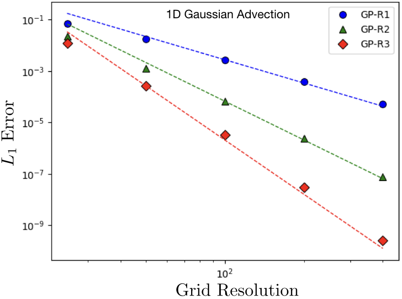
Figure 1: Plot of the $L_{1}$ errors for GP-WENO using R=1,2,3 on the 1D smooth Gaussian advection problem. Dotted lines show the corresponding $(2R+1)$ convergence rates.

Table 1: L1 errors for the 1D smooth Gaussian advection problem on five different grid resolutions. All simulations use $\ell=0.1$, $\sigma/\Delta=3$, and RK4 for time integration with an appropriately limited CFL condition to match the temporal and spatial accuracy.

Grid $\Delta$	GP-R1		GP-R2		GP-R3
	$L_{1}$	$L_{1}$ Order	$L_{1}$	$L_{1}$ Order	$L_{1}$	$L_{1}$ Order
1/25	$7.03\times 10^{-2}$	–	$2.25\times 10^{-2}$	–	$1.19\times 10^{-2}$	–
1/50	$1.74\times 10^{-2}$	2.02	$1.30\times 10^{-3}$	4.11	$2.64\times 10^{-4}$	5.49
1/100	$2.75\times 10^{-3}$	2.66	$6.70\times 10^{-5}$	4.28	$3.22\times 10^{-6}$	6.36
1/200	$4.01\times 10^{-4}$	2.78	$2.48\times 10^{-6}$	4.75	$2.97\times 10^{-8}$	6.76
1/400	$5.14\times 10^{-5}$	2.96	$7.84\times 10^{-8}$	4.99	$2.51\times 10^{-10}$	6.88

The length hyperparameter $\ell$ provides an additional knob to tune the solution accuracy. Fig. 2 shows how the $L_{1}$ error changes with the choice of $\ell$ on the 1D Gaussian advection problem for different resolutions using the 5th-order GP-R2 scheme compared to the 5th-order WENO-JS scheme (denoted with dotted lines). The dependence of the $L_{1}$ errors on $\ell$ is qualitatively similar for all resolutions. At larger values of $\ell$ (e.g., $\ell>0.3$) the errors begin to asymptotically plateau out and are generally higher than the corresponding WENO-JS simulation. This can be explained by the nature of the GP’s kernel-based data prediction, in which larger values of $\ell$ results in the GP model under-fitting the data. On the other hand, we see that all errors diverge at small $\ell$ (e.g., $\ell<0.1$) due to the fact that the GP model over-fits the data (i.e., large oscillations between the data points). The errors of GP-WENO reach a local minimum at $\sim\ell=0.1$, roughly the full-width half-maximum (FWHM) of the initial Gaussian density profile. In all cases this local minimum in the $L_{1}$ error is lower than the errors obtained using the WENO-JS scheme. This behavior is similar to that observed for radial basis function (RBF) methods for CFD [84], for the RBF shape parameter $\epsilon$ which represents an inverse length scale, i.e., $\epsilon\sim 1/\ell$. Nonetheless, the connection between the optimal $\ell$ and the length scales of the problem has only been made in the context of Gaussian process interpolations/reconstructions in our recent work [95]. This suggests that, to best resolve the “smallest” possible features in a simulation for a given grid spacing $\Delta$, the choice of $\ell\gtrsim\Delta$ may be optimal.

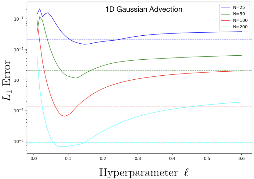
Figure 2: $L_{1}$ errors for different values of $\ell$ for the 1D Gaussian smooth advection. Solid lines show the GP-R2 scheme and dashed lines $L_{1}$ errors for the WENO-JS scheme using RK3 with a CFL=0.8.

6.2 2D Isentropic Vortex

Next, we test the accuracy of the GP-WENO schemes using the multidimensional nonlinear isentropic vortex problem, initially presented by Shu [104]. The problem consists of the advection of an isentropic vortex along the diagonal of a Cartesian computational box with periodic boundary conditions. We set up the problem as presented in [105], where the size of the domain is doubled to be $[0,20]\times[0,20]$ compared to the original setup in [104] to prevent self-interaction of the vortex across the periodic domain. The problem is run for one period of the advection through the domain until the vortex returns to its initial position, where the solution accuracy can be measured against the initial condition.

Our $L_{1}$ error results are shown in Fig. 3 and summarized in Table 2 using $\ell=1$, $\sigma/\Delta=3$, and RK4 for time integration, utilizing once more the appropriate reduction in time step to match the spatial and temporal accuracies. As with the 1D smooth advection in the previous section, the GP-WENO method obeys a $(2R+1)$ order of convergence rate.

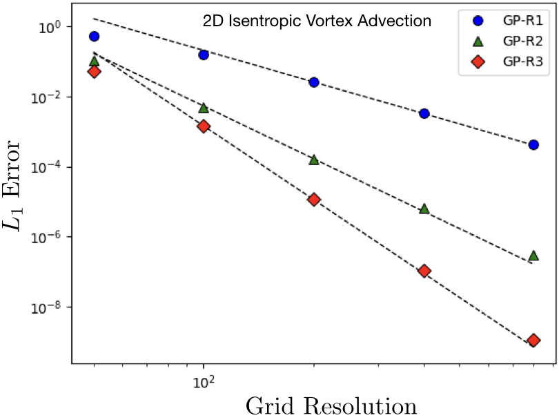
Figure 3: Plot of the $L_{1}$ errors for GP-WENO using R=1,2,3 on the isentropic vortex problem. Dotted lines show the corresponding $(2R+1)$ convergence rates. All simulations use $\ell=1.0$ and $\sigma/\Delta=3$. Temporal integration is done using RK4 with a suitably limited time step to match the temporal and spatial errors between different resolutions.

Table 2: $L_{1}$ errors for the 2D isentropic vortex problem. All simulations use $\ell=1.0$, $\sigma/\Delta=3$, and RK4 for time integration with an appropriately limited CFL condition to match temporal and spatial accuracy.

$\Delta$	GP-R1		GP-R2		GP-R3
	$L_{1}$	$L_{1}$ Order	$L_{1}$	$L_{1}$ Order	$L_{1}$	$L_{1}$ Order
2/5	$5.34\times 10^{-1}$	–	$1.33\times 10^{-1}$	–	$6.46\times 10^{-2}$	–
1/5	$1.60\times 10^{-1}$	1.74	$4.71\times 10^{-3}$	4.82	$1.14\times 10^{-3}$	5.82
1/10	$2.60\times 10^{-2}$	2.62	$1.54\times 10^{-4}$	4.93	$1.11\times 10^{-5}$	6.68
1/20	$3.38\times 10^{-3}$	2.94	$5.73\times 10^{-6}$	4.75	$1.03\times 10^{-7}$	6.75
1/40	$4.25\times 10^{-4}$	2.99	$2.34\times 10^{-7}$	4.61	$1.02\times 10^{-9}$	6.66

We also repeat the test of the dependence of the errors on the length hyperparameter $\ell$ and show the results in Fig. 4. Similar to the 1D case in Fig. 2 there is a minimum for the error at higher resolution around $\ell\gtrapprox 1$. The errors diverge at small values of $\ell$ and plateau at large $\ell$. Shown as dotted lines in Fig. 4 are the errors for the WENO-JS interpolation. For all resolutions, the minimum of the error for the GP-WENO scheme is significantly smaller than the errors of the WENO-JS scheme. This can also be seen by comparing the GP-R2 $L_{1}$ column of Table 2 to the WENO-JS $L_{1}$ column of Table 3. Also, the order of convergence for the WENO-JS is smaller than that of GP-R2 method.

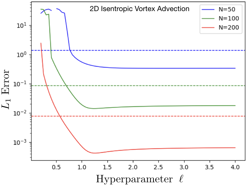
Figure 4: $L_{1}$ errors for different values of $\ell$ for the 2D isentropic vortex problem using $\sigma/\Delta=3$. Dotted lines show the WENO-JS $L_{1}$ errors at the same resolutions.

Table 3: $L_{1}$ errors or the 2D isentropic vortex using WENO interpolations comparing the choice of smoothness indicators. WENO-JS indicates the use of the classical polynomial-based smoothness indicators and WENO-GP indicates the use of the new GP-based smoothness indicators.

$\Delta$	WENO-JS		WENO-GP
	$L_{1}$	$L_{1}$ Order	$L_{1}$	$L_{1}$ Order
2/5	$8.68\times 10^{-2}$	–	$8.10\times 10^{-2}$	–
1/5	$3.28\times 10^{-3}$	4.72	$4.83\times 10^{-3}$	4.07
1/10	$5.81\times 10^{-4}$	2.50	$1.73\times 10^{-4}$	4.80
1/20	$3.83\times 10^{-5}$	3.92	$7.41\times 10^{-6}$	4.55
1/40	$1.69\times 10^{-6}$	4.50	$2.69\times 10^{-7}$	4.78

We attribute the significant improvement in errors for the GP-R2 scheme over the classical WENO-JS to the use of the GP-based smoothness indicators in Eq. (36), which seem to better suit the adaptive stencil process in WENO-type methods for nonlinear problems like the isentropic vortex test. It is known that the original weighting scheme of the WENO-JS method [41] suffers from reduced accuracy in the presence of inflection points that lowers the scheme’s formal order of accuracy. This has been addressed with such schemes as the Mapped WENO [106] or the WENO-Z [107] methods. All of these methods use the same smoothness indicators as in WENO-JS and acquire improved behavior by modifying the way nonlinear weights are formulated (see Eq. (33)). The GP-WENO method uses exactly the same weighting as in the classical WENO-JS scheme and the observed improvement originates from the new GP-based smoothness indicators.

This suggests that the GP-based smoothness indicators could also be applied in conventional polynomial-based WENO interpolations/reconstructions to achieve improved accuracy in smooth solutions. More specifically, a WENO polynomial-interpolation is used for $\mathbf{f}_{m}$ on the candidate stencils $S_{m}$ (Eq. (26)), while the GP-based smoothness indicators are adopted in Eq. (36). We refer to such a scheme as the WENO-GP weighting scheme. In Table 3, we compare $L_{1}$ errors for the WENO-JS and WENO-GP schemes. The latter outperforms the former, without changing the formulation of the weights $\tilde{\omega}_{m}$.

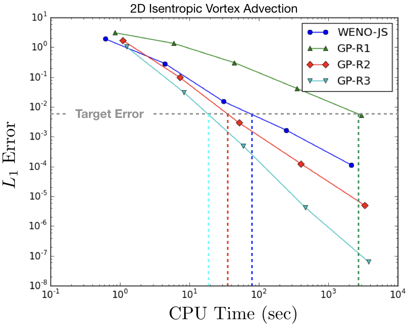
Figure 5: $L_{1}$ errors vs. CPU time (sec) for the 2D isentropic vortex problem on $[0,20]\times[0,20]$, parallelized on four compute cores (2.7 GHz 12-Core Intel Xeon E5). The results were obtained using CFL=0.4 and temporally integrated using RK4 without any use of timestep reduction. The two hyperparameters were set as $\ell=1.2$ and $\sigma/\Delta=3$. An HLLC Riemann solver was used in all cases. The dotted horizontal line is the target $L_{1}$ error of $5\times 10^{-3}$.

In Fig. 5 we show the CPU efficiency of WENO-JS and of GP-WENO with $R=1,2$, and $3$ as the $L_{1}$ error versus the CPU time for the isentropic vortex problem. The 5th-order GP-R2 and 7th-order GP-R3 schemes yield faster time-to-solution accuracy when compared to the 5th-order WENO-JS scheme. The comparison is quantitatively summarized in Table 4.

Table 4: Relative CPU time for the four schemes to reach the target $L_{1}$ error of $5\times 10^{-3}$, represented by the dotted horizontal line in Fig. 5. All CPU times are normalized to that of WENO-JS.

Scheme	Relative time-to-error
GP-R1	35.81
GP-R2	0.43
GP-R3	0.22
WENO-JS	1.0

7 Numerical Test Problems with Shocks and Discontinuities

In this section we present test problems using the GP-WENO interpolation method described in Section 3 and applied to the compressible Euler equations in 1, 2, and 3D. The GP-WENO with $R=2$ (or GP-R2) scheme is chosen as the default method and is compared to the 5th order WENO method [60, 41, 57] that is nominally of the same order of accuracy. All interpolations are carried out on characteristic variables to minimize unphysical oscillations in the presence of discontinuities [108] . A 3rd-order TVD Runge-Kutta method (RK3) [96] for temporal integration and an HLLC [109, 70] Riemann solver are used throughout unless otherwise specified. The two hyperparameters $\ell$ and $\sigma$ are chosen to have values so that $\ell/\Delta\sim 6-12$ and $\sigma/\Delta\sim 1.5-3$.

7.1 1D Scalar Advection

Our first test is the scalar advection problem of [41], which consists of passive advection of several shapes through a periodic domain. The profiles consist of a combination of (i) a Gaussian, (ii) a square pulse, (iii) a sharply peaked triangle and (iv) a half-ellipse from left to right. We follow [41] to set up the problem on a grid with 200 points and evolve the solution up to a final time of $t=8$, which corresponds to 4 periods through the domain. Results comparing the WENO-JS and GP-R2 methods for this problem are shown in Fig. 6a using the GP-WENO scheme with the smoothness indicators outlined in Eq. (36). The GP-R2 solution captures the amplitudes of the Gaussian and triangle waves more effectively than does the WENO-JS solution. However, for the square wave the GP-R2 solution introduces some Gibbs phenomena at the discontinuities. Similar oscillations associated with flat discontinuities like those shown here have been also observed in shock-tube problems in our previous finite volume version of GP-WENO [95]. We find that this issue stems from the use of the zero-mean prior in the calculation of the smoothness indicators, which biases the stencil choice towards those that are more compatible with the zero-mean prior (i.e., data that are closer to zero). The issue can be alleviated by setting a non-zero mean using the cell-centered data $\mathbf{f}_{i}$ on the cell $I_{i}$ in Eq. (36), changing from $\mathbf{f}_{m}$ to $(\mathbf{f}_{m}-\mathbf{f}_{i})$. A solution obtained using these smoothness indicators for GP-R2 is shown in Fig. 6b. While this greatly improves GP-WENO’s performance on this scalar advection problem, the non-zero mean can have some unintended consequences on multidimensional problems. Because the smoothness indicators with non-zero means $\mathbf{f}_{i}$ are computed using the residuals of the data, $\mathbf{f}_{m}-\mathbf{f}_{i}$, the stencil adaptation could become sensitive to machine precision differences in the data on a stencil. Such differences could potentially lead to an instability in the stencil selection. In problems that contain a specific symmetry, such as the 2D Riemann Problem presented in Sec. 7.6, machine precision asymmetries in the initial conditions can be observed to be amplified significantly in a runaway process due to an asymmetry in the stencil adaptation in the WENO procedure. In practice, for all nonlinear problems tested in this paper, the oscillations from the zero mean choice are relatively small and so the choice of zero mean is used in the remainder of the results presented.

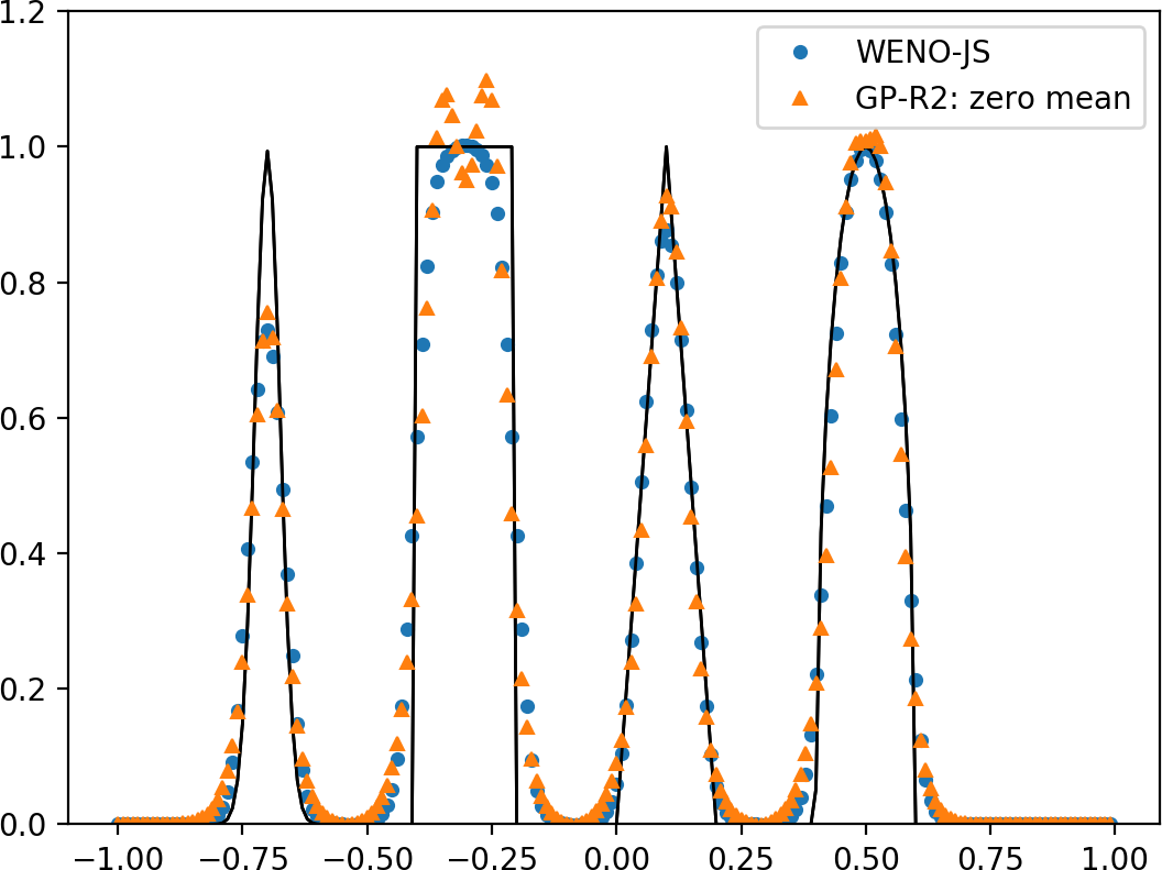
(a)

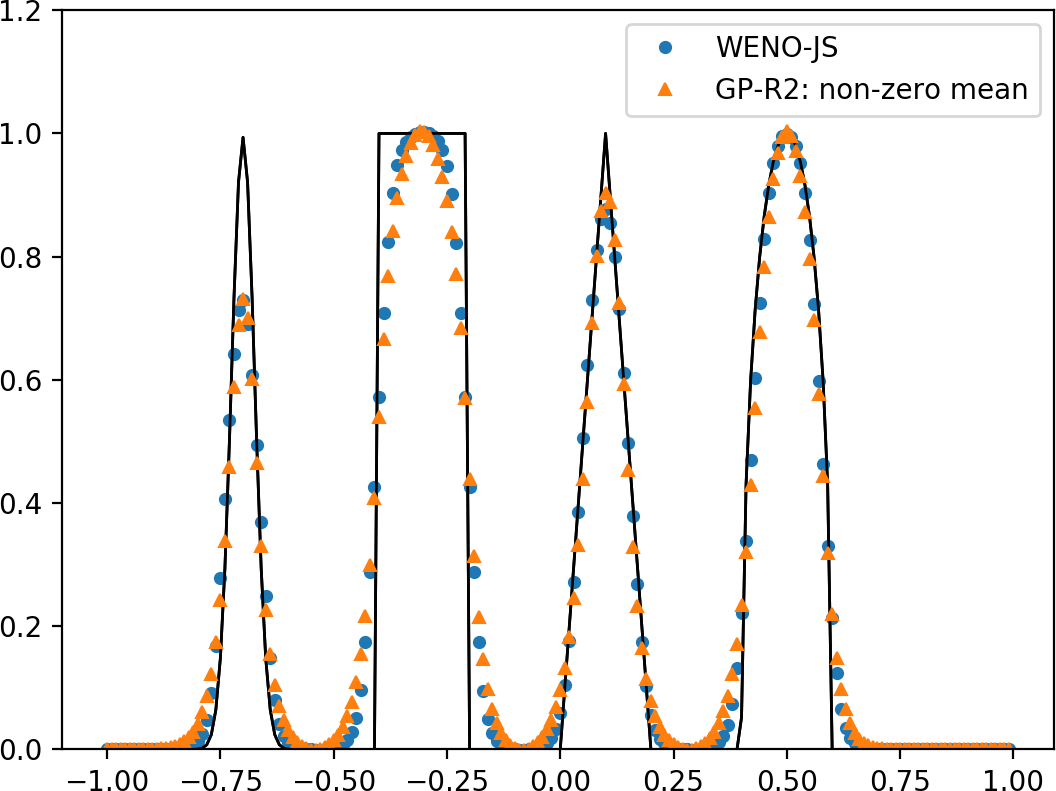
(b)

Figure 6: WENO-JS and GP-WENO solutions for the scalar advection problem obtained on a 200 point grid up to $t=8$ with a CFL of 0.4. GP-WENO solutions used values of $\ell/\Delta=12$ and $\sigma/\Delta=3$. The left panel 6a shows a GP-WENO solution using a zero mean in the calculation of the smoothness indicators, and the right panel 6b shows a GP-WENO solution obtained using a non-zero mean.

7.2 1D Shu-Osher Problem

The Shu-Osher problem [62] is a compound test of a method accuracy and stability. The goal is to resolve small scale features (i.e., high-frequency waves) in a post-shock region and concurrently capture a Mach 3 shock in a stable and accurate fashion.

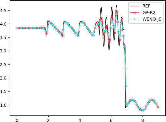
(a)

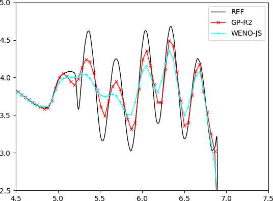
(b)

Figure 7: (Left) The Shu-Osher problem at $t=1.8$ using RK3 and the HLLC Riemann solver. The GP-R2 scheme is shown in red, using $\ell/\Delta=6$ and $\sigma/\Delta=3$. The WENO-JS scheme is shown in cyan. Both schemes are resolved on 200 grid points using a CFL of 0.8. The reference solution (black) is obtained using WENO-JS on a resolution of 2056 grid points. (Right) Close-up of the frequency-doubled oscillations.

In this problem, a (nominally) Mach 3 shock wave propagates into a constant density field with sinusoidal perturbations. As the shock advances, two sets of density features develop behind the shock: one that has the same spatial frequency as the initial perturbation; one that has twice the frequency of the initial perturbations and is closer to the shock. The numerical method must correctly capture the dynamics and the amplitude of the oscillations behind the shock, and be compared against a reference solution obtained using much higher resolution.

(a)

(b)

Figure 8: Comparison for different values of $\ell$ and $\sigma$ of the GP-R2 (8a) and GP-R3 (8b) schemes on the Shu-Osher problem on 200 grid points. The reference solution is shown in black.

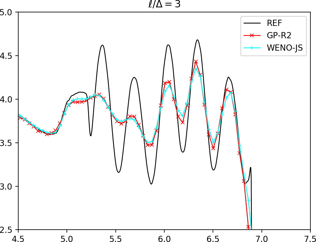
(a)

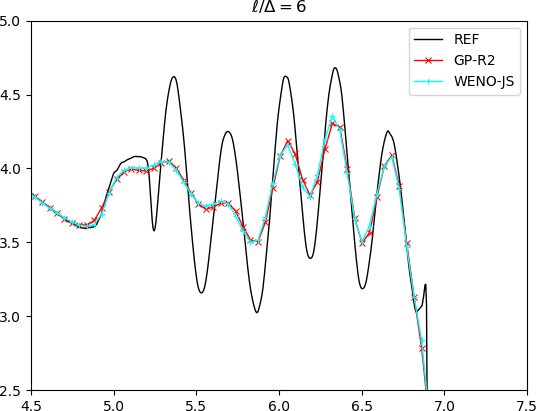
(b)

Figure 9: Close-ups of the Shu-Osher problem using GP interpolation with the WENO-JS smoothness indicators instead of the default GP-based smoothness indicators.

The results for this problem are shown in Fig. 7a for the whole domain (left). A close-up of the frequency doubled oscillations is shown in Fig. 7b. We compare the GP-R2 method, with $\ell/\Delta=12$ and $\sigma/\Delta=3$, to the WENO-JS method. The GP-R2 scheme clearly captures the amplitude of the oscillations better than the 5th order WENO-JS. Again, the improvement over the WENO-JS scheme is attributed to the use of the GP smoothness indicators.

Fig. 8 shows the Shu-Osher problem for the 5th order GP-R2 and the 7th order GP-R3 schemes, for different values of $\ell$ and $\sigma$. Changing $\ell$ results in small changes in the amplitude of the oscillations, while the variation of $\sigma$ has a more significant impact. Smaller values of $\sigma/\Delta$ result in more oscillations, while larger values better match the reference solution. From this parameter study we conclude that $\sigma/\Delta=3$ is fairly a robust choice for this shock tube problem. Further, we found that $\sigma/\Delta$ can be further reduced closer to $\sim 1.5$ on higher resolution runs and in problems with stronger shocks.

In Fig. 9 we show the combination of the GP-R2 interpolation with the classical WENO smoothness indicators. The FWHM of the post shock oscillations is $\sim 3-4$ times the grid spacing $\Delta$. This suggests that, following the FWHM discussion in Section 6, a choice of $\ell/\Delta=3$ for GP-R2 is optimal. This is confirmed in Fig. 9, where the solution in panel (a) with $\ell/\Delta=3$ better captures the amplitude of the oscillations, when compared to WENO-JS and the GP-R2 solution with $\ell/\Delta=6$. Notwithstanding, the default combination of GP-based smoothness indicators with GP-WENO yields much better results overall (Fig. 7b).

7.3 1D Two Blast Wave Interaction

This problem was introduced by Woodward and Colella [110] and consists of two strong shocks interacting with one another.

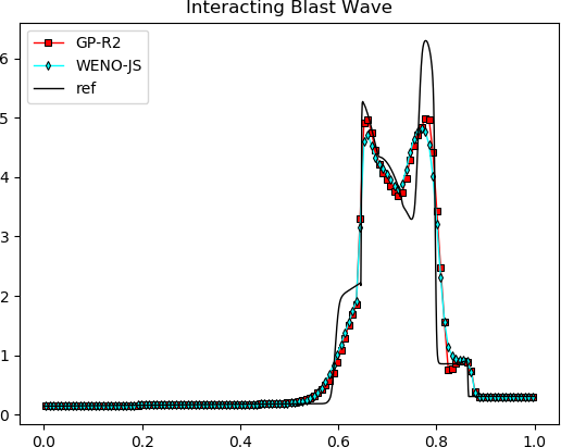
(a)

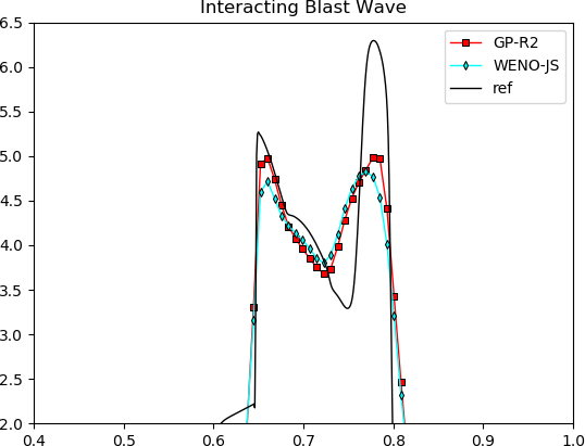
(b)

Figure 10: (a) Two blast interaction problem showing GP-R2 (red) with $\ell/\Delta=12$ and $\sigma/\Delta=3$ and WENO-JS (cyan) on 128 points using a CFL of 0.8. (b) Zoom-in of the shock-interaction region.

We follow the original setup of the problem and compare the GP-R2 scheme with the 5th order WENO-JS schemes on a computational domain of $[0,1]$, resolved onto 128 grid points. We set $\ell/\Delta=12$ and $\sigma/\Delta=3$. Fig. 10 shows the density profiles for GP-R2 and WENO-JS at $t=0.038$, compared against a highly-resolved WENO-JS solution (2056 grid points). As shown in Fig. 10a, both methods yield acceptable solutions. However, the close-ups in Fig. 10b reveals that the GP-R2 scheme better resolves the peaks and is closer to the reference solution.

7.4 2D Sedov

Next, we consider the Sedov blast test [111]. This problem studies the methods ability to maintain the symmetry of the self-similar evolution of a spherical shock, generated by a high pressure point-source at the center of the $[-0.5,0.5]\times[-0.5,0.5]$ domain. We follow the setup of [112].

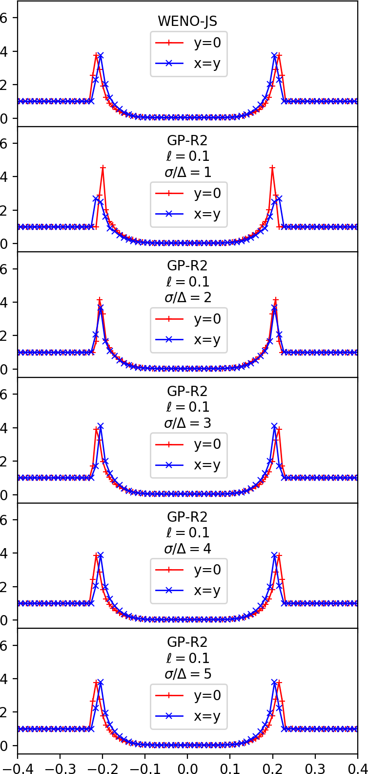
(a)

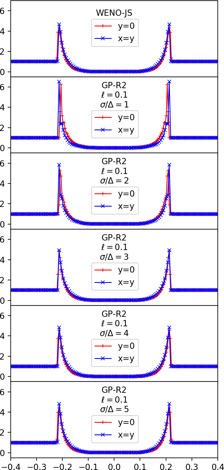
(b)

Figure 11: Comparison of $\sigma/\Delta$ values on two resolutions, $128\times 128$ (11a) and $256\times 256$ (11b), using GP-R2 for the Sedov problem. Shown are the density profiles along the $x$-axis (red) and along the diagonal $y=x$ (blue).

Fig. 11 shows density profiles along $y=x$ (i.e., the diagonal) and $y=0$ (i.e., the $x$-axis) with GP-R2, at two different resolutions ($128\times 128$ and $256\times 256$) and different choices of $\sigma/\Delta$. All runs used a value of $\ell=0.1$ to perform a parameter scan on $\sigma/\Delta$. The top two panels show the solutions obtained with WENO-JS. Again, as in the Shu-Osher problem, small values of $\sigma/\Delta$ introduce oscillations and lead to asymmetric shock evolution, whereas a choice of $\sigma/\Delta=3$ gives a good balance.

7.5 2D Mach 3 Wind Tunnel with a Step

The next 2D shock problem consists of a Mach 3 wind tunnel setup with a forward facing reflecting step, originally proposed by Woodward and Colella [110]. We initialize the problem as in [110] with an entropy fix for the region immediately above the corner of the step. After the bow shock reflects on the step, the shock progressively reaches the top reflecting wall of the tunnel at around $t=0.65$. A triple point is formed due to the reflections and interactions of the shocks, from which a trail of vortices travels towards the right boundary.

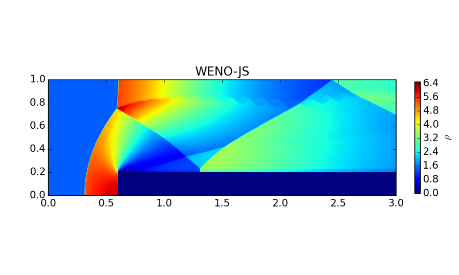
(a)

(b)

(c)

Figure 12: Three density profiles for the Mach 3 wind tunnel problem with a step are shown: (a) the WENO-JS scheme (b) the GP-R2 scheme; (c) the GP-R3 scheme. The domain is resolved onto a $768\times 256$ grid. We use an HLL Riemann solver and RK3, with a CFL of $0.4$. The temporal evolution is followed up to $t=4$. The two GP runs in (b) and (c) used $\sigma/\Delta=2$ and $\ell/\Delta=12$.

Shown in Fig. 12 are the results computed using the GP-R2 and GP-R3 schemes, along with the WENO-JS solution on a $768\times 256$ grid at the final time $t=4$. Using the HLLC Riemann solver, we noticed that the GP and WENO-JS schemes converged to different solutions, on account of the singularity at the corner of the step and despite the entropy fix. To compare the two schemes, we ran our simulations using an HLL Riemann solver, for which the two schemes converged to similar solutions. Both methods are able to capture the main features of the flow but the GP schemes produce more well-developed Kelvin-Helmholtz roll-ups that originate from the triple point.

7.6 2D Riemann Problem – Configuration 3

Next, we consider a specific Riemann Problem configuration that is drawn from a class of two dimensional Riemann problems that have been studied extensively [113, 114] and have been applied to code verification efforts [43, 115, 116, 117, 118, 46]. Specifically, we look at the third configuration of the 2D Riemann problem presented in [118, 46].

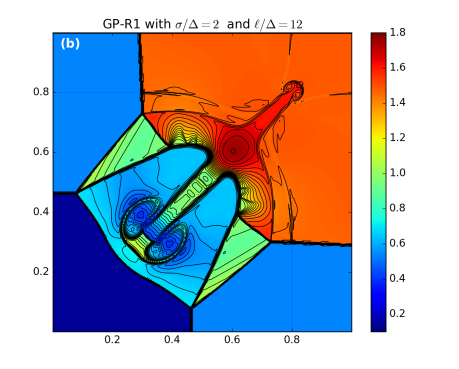
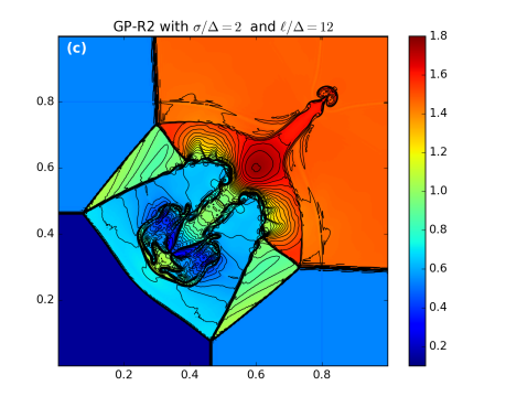
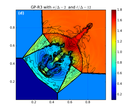
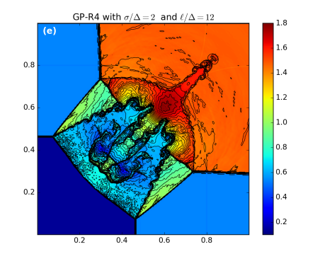
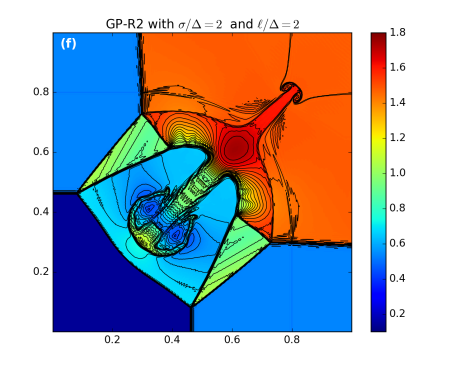
Figure 13: Configuration 3 of the 2D Riemann problem using four different methods: (a) WENO-JS, (b) GP-R1, (c) GP-R2, (d) GP-R3, (e) GP-R4, where (b) – (e) have $\sigma/\Delta\neq\ell/\Delta$, and finally, (f) GP-R2 with $\sigma/\Delta=\ell/\Delta$. Each panel shows the density values at $t=0.8$ between $[0.1,1.8]$ in linear scale, computed on a $400\times 400$ grid. We over-plot 40 contour lines. All GP calculations used $\ell/\Delta=12$ except for (f). An HLLC Riemann solver and RK3 were employed in all calculations, with CFL=0.4.

Panels in Fig. 13 show density profiles at $t=0.8$, along with 40 contour lines, for different choices of GP radii, $R=1,2,3,4$ on a $400\times 400$ grid resolution. All GP methods correctly capture the expected features of the problem. In this experiment, we see that the increase of $R$ results in a sharper representation of the flow features. Notably, the 5th-order GP-R2 solution in (c) captures significantly more features when compared to the 5th-order WENO-JS in (a), as evinced by the formation of more developed Kelvin-Helmholtz vortices along the slip lines (i.e., the interface boundaries between the green triangular regions and the sky blue areas surrounding the mushroom-shaped jet).

7.7 Double Mach Reflection

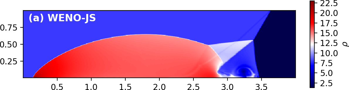
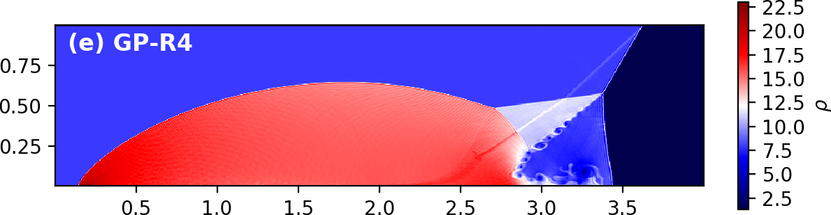
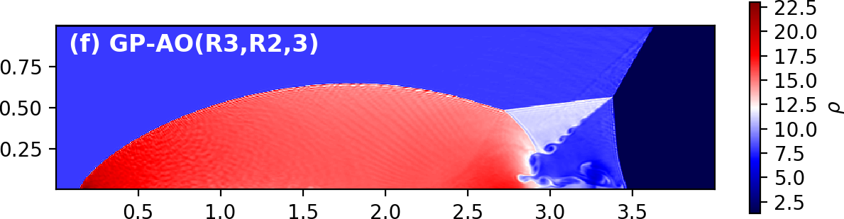
Figure 14: The double Mach reflection (DMR) problem solved using six different methods, (a) WENO-JS, (b) GP-R1, (c) GP-R2, (d) GP-R3, (e) GP-R4, and (f) GP-AO($R3$,$R2$,3). We show density plots at $t=0.25$. The calculations were performed on a $800\times 200$ grid, with $\ell/\Delta=12$ and $\sigma/\Delta=1.8$. For all cases we used the HLLC Riemann solver, RK3, and CFL=0.4.

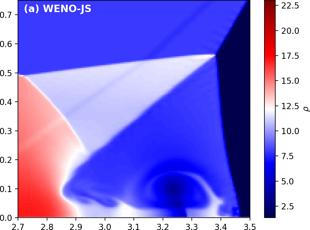
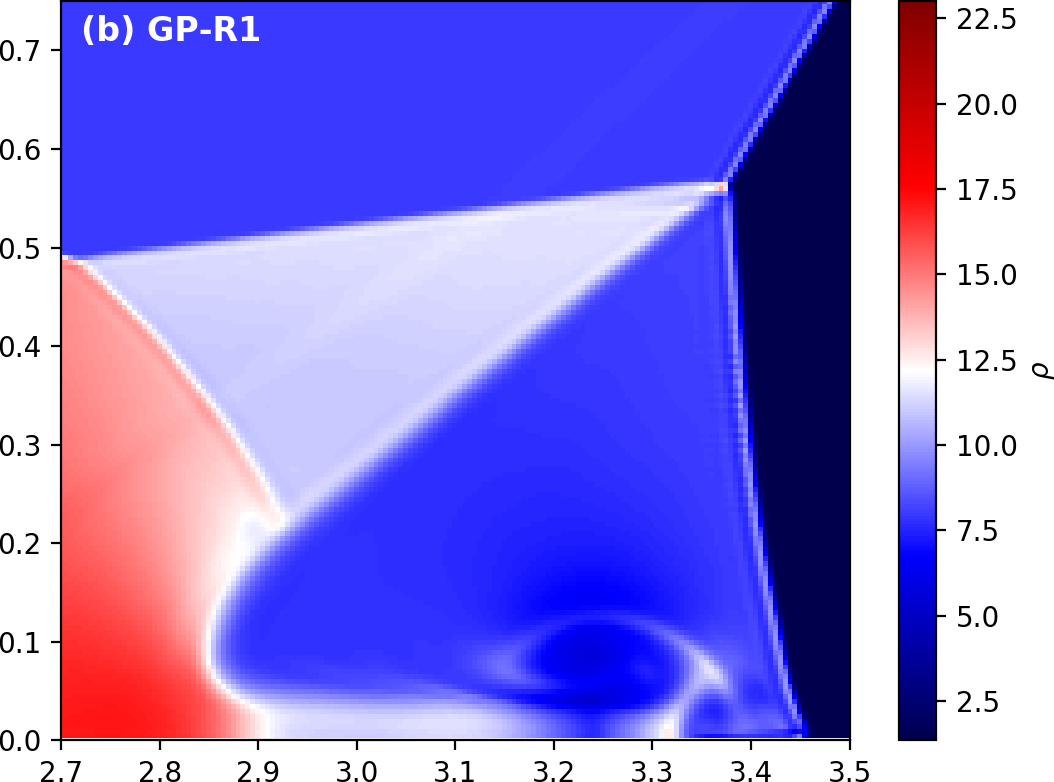
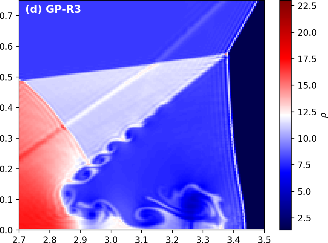
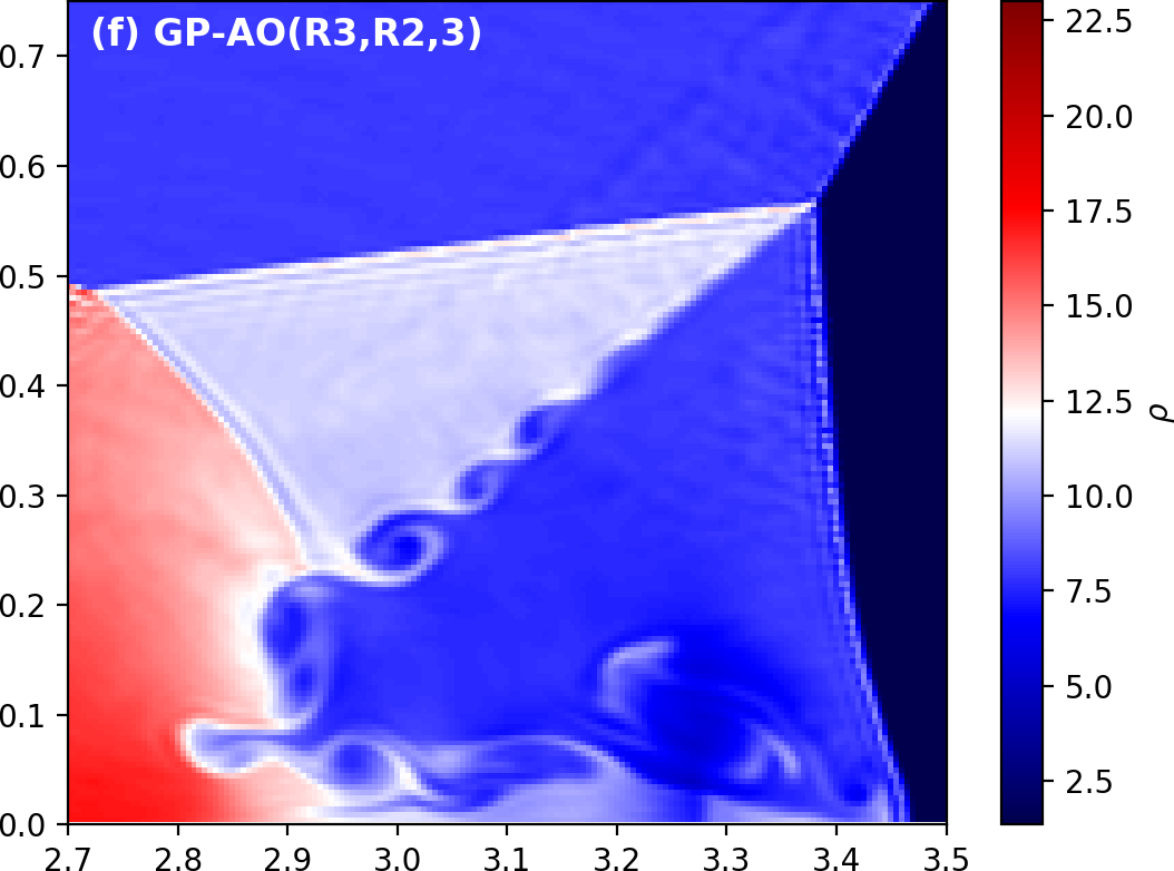
Figure 15: Close-ups near the triple point of the density profiles of Fig.  14.

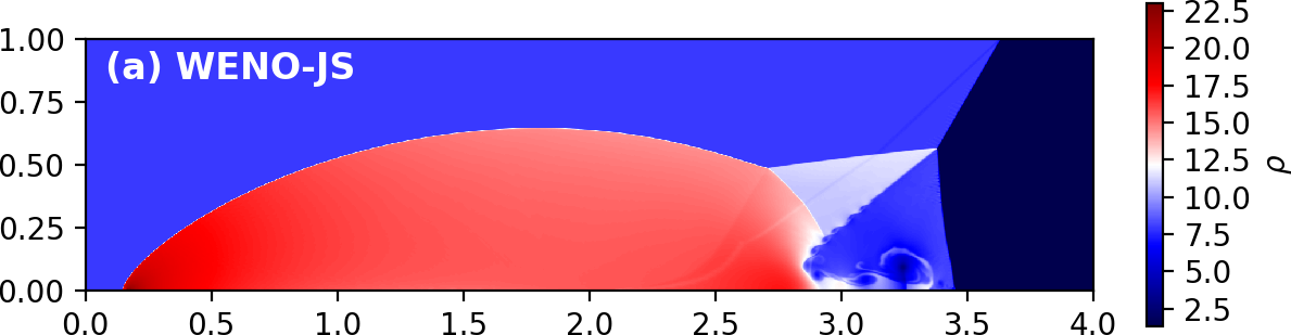
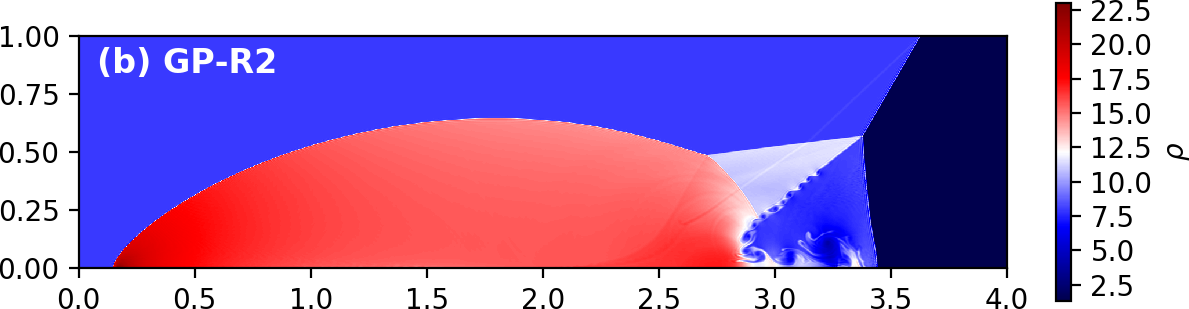
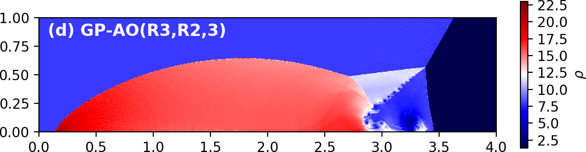
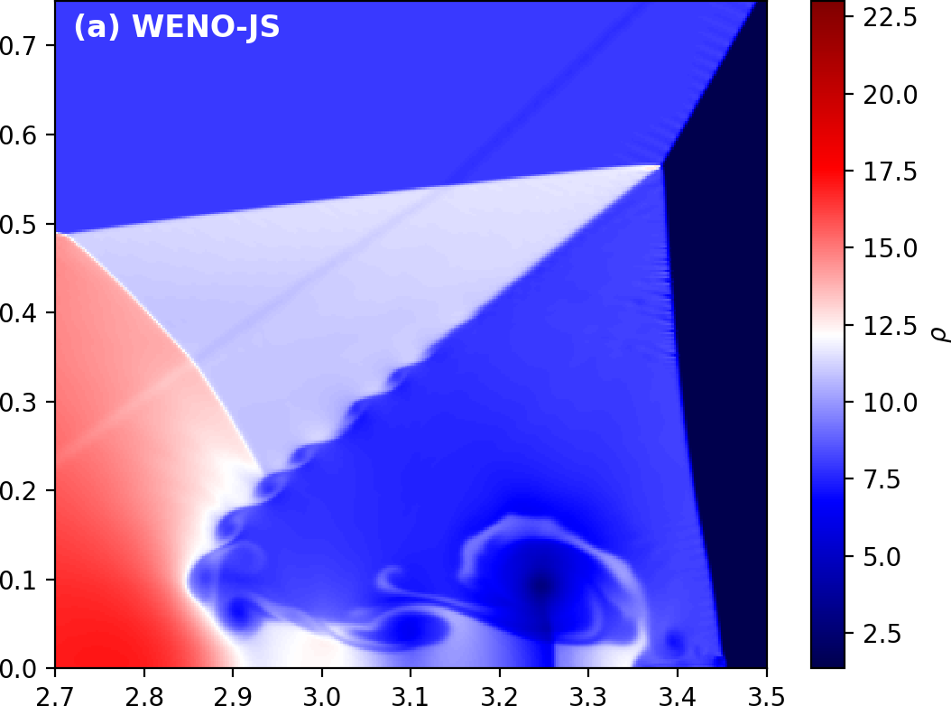
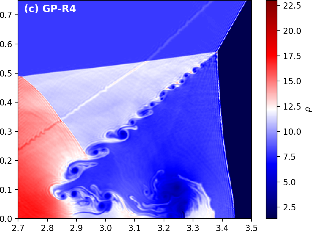
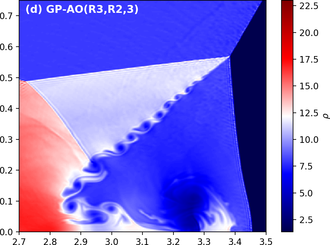
Figure 16: The density profiles of the DMR test performed on a high-resolution grid ($1600\times 400$). (a) WENO-JS, (b) GP-R2, and (c) GP-R4, and (d) GP-AO($R3$,$R2$,3), with $\sigma/\Delta=1.8$ and $\ell/\Delta=12$ for cases (b) to (d). The four bottom panels are close-ups of the top four panels near the triple point. For all cases we used the HLLC Riemann solver, RK3, and CFL=0.4.

Our last 2D test is the double Mach reflection problem introduced by Woodward and Colella [110]. This test problem consists of a strong Mach 10 shock that is incident on a reflecting wedge that forms a $60^{\circ}$ angle with the plane of the shock. Fig. 14 shows density profiles from $800\times 200$ grid resolution runs, for a variety of GP stencil radii ($R=1,2,3,4$), as well as for the GP adaptive order (AO) hybridization [100] (detailed in A). We present these GP solutions together with a 5th-order WENO-JS solution for comparison. The reflection of the shock at the wall forms two Mach stems and two contact discontinuities. The contact discontinuity that emanates from the roll-up of the stronger shocks is known to be Kelvin-Helmholtz unstable provided there is sufficiently low numerical dissipation in the method. Thus, the problem quantifies the method’s numerical dissipation by the number of Kelvin-Helmholtz vortices present at the end of the run.

The presence of a highly supersonic shock is a stringent test for the stability of the algorithm. We find that the GP solutions remain stable for small values of $\sigma/\Delta$. The choice of $\ell/\Delta$ does not appear to considerably affect stability and thus can be set to relatively larger values than $\sigma/\Delta$. All GP runs successfully reach $t=0.25$ for $\sigma/\Delta=1.8$ and $\ell/\Delta=12$ on two different resolutions, $800\times 200$ in Fig. 14 and $1600\times 400$ in Fig. 16.

Close-ups in Fig. 15 reveal that GP-WENO is significantly better at capturing the development of Kelvin-Helmholtz vortices in the Mach stem than the WENO-JS method. More specifically, the 5th order GP-R2 scheme is less dissipative than the WENO-JS scheme, which in turn is less dissipative than the 3rd order GP-R1 scheme. Both 7th order GP-R3 and 9th order GP-R4 schemes are able to resolve more vortices. While the GP-AO($R3,R2,3$) scheme is less dissipative than the GP-R2, it does not capture as many features as the GP-R3 scheme. This is despite the fact that both GP-AO($R3,R2,3$) and GP-R3 are of the same formal order of accuracy in smooth flows.

In Fig. 16 we provide results for double the grid resolution, $1600\times 400$. The ranking derived from the lower resolution solutions still holds and the reduced dissipation of the GP-R2 scheme over the 5th order WENO-JS is more evident. Further, the GP-R3 on the $800\times 200$ grid in Fig. 15(d) captures more vortices than WENO-JS on the $1600\times 400$ grid in Fig. 16(a). Our results from Fig. 16 can be directly compared to one of the most recent finite difference WENO-AO solutions by Balsara et al. [100] (see their Fig. 7).

7.8 3D Explosion

This 3D explosion test problem was introduced by Boscheri and Dumbser [119] as a three-dimensional extension of the Sod problem [120]. The test is set up on a $[-1,1]\times[-1,1]\times[-1,1]$ domain with outflow boundary conditions. The initial condition is given by

$$\mathbf{V}(\mathbf{x})=\left\{\begin{array}[]{clrrl}\mathbf{V}_{\text{i}}&=\;(1,0,0,0,1)&\text{if }||\mathbf{x}||\leq R,\\ \mathbf{V}_{\text{o}}&=\;(0.125,0,0,0,0.1)&\text{if }||\mathbf{x}||>R,\end{array}\right.$$ (37)

where $\mathbf{V}=(\rho,u,v,w,P)$ and $R=0.5$. The ratio of specific heats is $\gamma=1.4$ and the simulation completes at $t=0.25$.

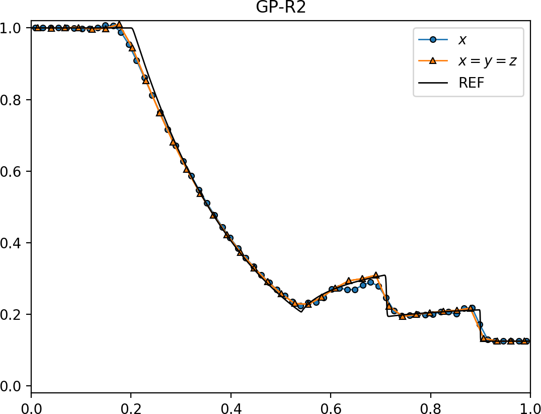
(a)

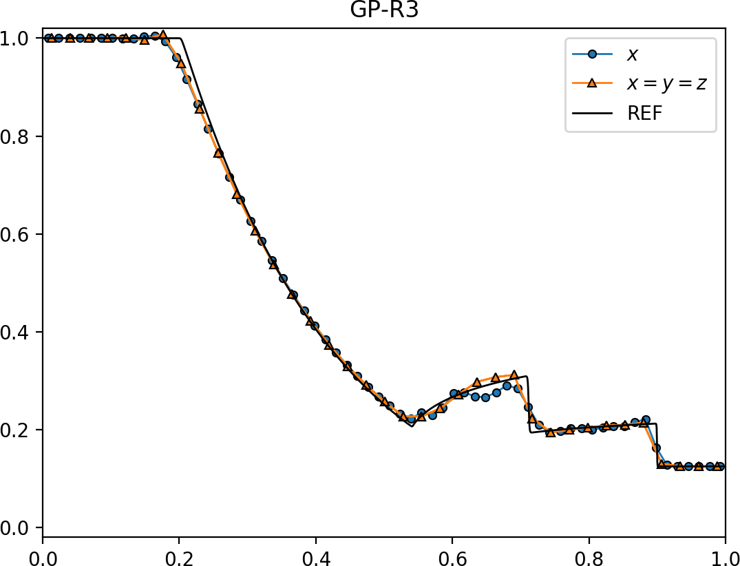
(b)

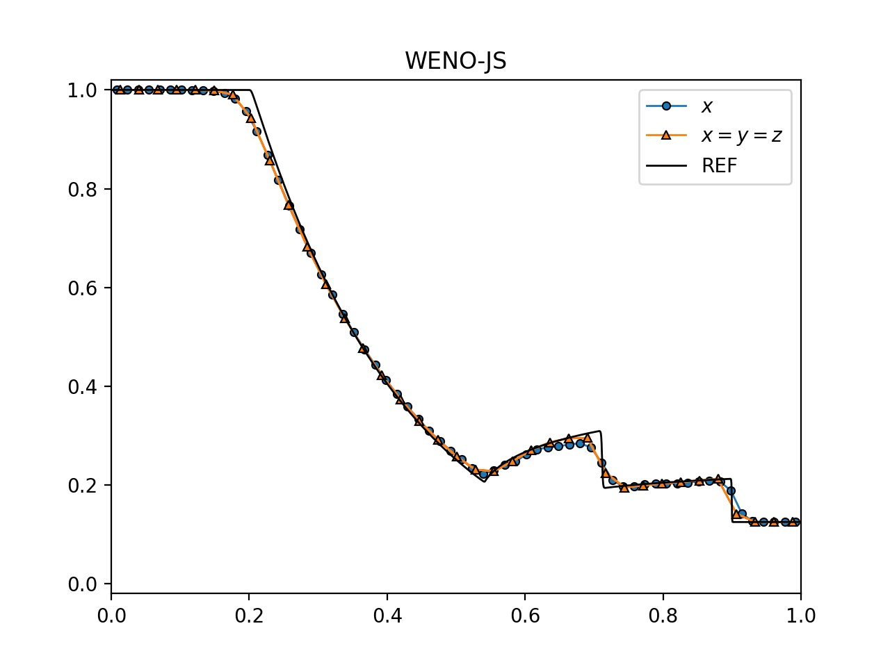
(c)

Figure 17: Radial density profiles along the $x$-axis and the diagonal $x=y=z$, for GP-R2, GP-R3 and WENO-JS on a $128\times 128\times 128$ grid, using a CFL of 0.3, HLLC, and RK3. GP simulations use $\ell/\Delta=12$ and $\sigma/\Delta=3$.

Fig. 17 shows the resulting density profiles for the GP-R2 and WENO-JS schemes, along with a reference solution. The latter is obtained by considering the simplification of the spherically symmetric Euler equations as a 1D system with geometric source terms on 2056 grid points. Both methods produce well-acceptable solutions. We observe that the GP-R2 solution produces some minor under- and over-shooting along the coordinate axes, which however did not affect the stability of the calculation.

7.9 3D Riemann Problem

Finally, we consider the first configuration of the 3D Riemann problem presented in [121]. The problem consists of eight constant initial states in one octant of the $[-1,1]\times[-1,1]\times[-1,1]$ computational domain, with outflow boundary conditions. This initial condition provides a set of 2D Riemann problems on each face of the domain, as well as on its diagonal planes.

The results for the GP-R2, GP-R3, and WENO-JS schemes are shown respectively in Figs. 18, 19, and 20. In the left panels of the figures we discern three of the 2D Riemann problems, on the visible faces of the domain and on the plane in the $(1,1,0)$ direction. The latter is also shown in the right panels of figures, along with contour lines. The GP methods are able to adequately capture the important features of the 2D Riemann problems to approximately the same extent. Both GP solutions are better at resolving the contact discontinuity along the diagonal, when compared to the WENO-JS solution (see right panels of Figs. 18-20). All calculations here employed the HLLC Riemann solver, RK3, and a CFL of 0.3.

(a)

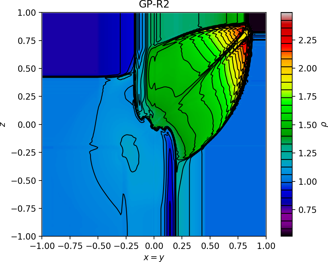
(b)

Figure 18: (a) 3D Riemann problem density profiles on the domain faces and on the plane in the (1,1,0) direction using GP-R2. We use $\ell/\Delta=12$, $\sigma/\Delta=3$, a grid resolution of $200\times 200\times 200$, and a CFL of $0.3$. (b) Density profile on the plane in the (1,1,0) direction.

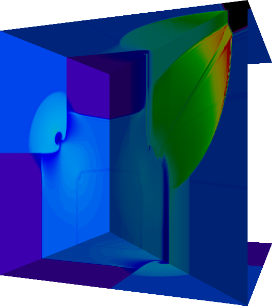
(a)

(b)

Figure 19: (a) Same as Fig. 18a but for GP-R3. (b) Same as Fig. 18b but for GP-R3.

(a)

(b)

Figure 20: (a) Same as Fig. 18a but for WENO-JS. (b) Same as Fig. 18b but for WENO-JS.

8 Conclusion

In this paper we have extended the 1D GP-WENO FVM reconstruction from [95] to operate as a high order interpolant for the FD-Prim method for solving hyperbolic systems of full three-dimensional conservation laws. To better capture shocks and discontinuities, we have refined the GP-WENO smoothness indicators, based on the GP log-likelihood, to use a separate length hyperparameter $\sigma$ from the actual GP data interpolation.

The use of GP interpolation, along with GP-based smoothness indicators, has shown fast rates of convergence in solution accuracy for smooth problems, which can be variably controlled by the parameter $R$. We demonstrated that the order of solution accuracy of the GP-WENO FD-Prim method varies linearly as $(2R+1)$ on smooth flows within one single algorithmic framework. By being a polynomial-free method, GP-WENO does not require the formulation or implementation of separate numerical algorithms as the order of accuracy varies. This is not the case for most conventional polynomial-based approaches as one needs to formulate a different piecewise polynomial algorithm for a given order, introduce additional basis functions, and approach it in terms of the grid $\Delta$ and the local stencil size. In this context, the GP-WENO formulation is more flexible and less deterministic in providing a variable range of solution accuracies, since the model is specified by its kernel function rather than explicit polynomial basis functions. This novel, variable, high-order scheme allows for flexible algorithmic design with minimal complexity and, at the same time, is able to captures shocks and discontinuities in a non-oscillatory, stable manner.

Moreover, our GP-based smoothness indicators are able to provide higher solution accuracy relative to the standard WENO-based smoothness indicators with the same weighting scheme. The solution accuracy can be tuned further using the kernel hyperparameter $\ell$, which provides an additional knob for increased accuracy that is not available in traditional polynomial-based methods.

Finally, the GP-based smoothness indicators can be implemented as a standalone numerical algorithm to be integrated in any conventional polynomial-based WENO scheme, enhancing its solution accuracy.

9 Acknowledgements

This work was supported in part by the National Science Foundation under grant AST-0909132, in part by the U.S. DOE NNSA ASC through the Argonne Institute for Computing in Science under field work proposal 57789, and in part by the Hellman Fellowship Program at UC Santa Cruz. We acknowledge support from the U.S. DOE Office of Science under grant DE-SC0016566 and the National Science Foundation under grant PHY-1619573. The authors also thank anonymous referees for their helpful suggestions and comments on our manuscript, which led us to improve the paper during the review process.

Appendix A Adaptive Order (AO) GP

In this Appendix, we provide a hybrid scheme for handling discontinuities in a non-oscillatory fashion, while keeping the desired high-order of accuracy away from shocks and discontinuities. The approach we describe here is called the adaptive order (AO) approach recently proposed by Balsara et al. [100]. The main idea behind the adaptive order approach is to nonlinearly hybridize a lower-order interpolation that favors stability over accuracy with a higher-order interpolation on a large stencil. The hybridization is performed in such a way that it biases towards the stable lower-order interpolation in the presence of discontinuities, while the higher-order one is preferred in smooth regions.

To begin, we start with a high-order GP interpolation of a Riemann state $q^{R}_{*}$, given by Eq. (20) on a stencil $S_{R}$ of radius $R>1$. The stencil $S_{R}$ also comes with a smoothness indicator $\beta^{R}$, given by the log-likelihood in Eq. (34). It is important to note that, for the AO formulation, we will be comparing stencils of different size. Thus, unlike the GP-WENO formulation discussed in Section 3, it will be necessary to retain the normalization and complexity penalty terms (i.e., the first and the second terms) that are in Eq. (34). We aim to nonlinearly hybridize the high-order interpolation $q_{*}^{R}$, with a lower-order, stable interpolation which we will call $q_{*}^{C}$.

We now describe how to obtain the lower-order stable interpolation $q_{*}^{C}$. The choice of linear weights given by Eq. (28) or in the original WENO-JS scheme [41] are designed to be optimal only in the sense of accuracy. Other types of WENO schemes can be formed that prefer stability over accuracy, such as the central WENO (CWENO) schemes [122, 123, 124]. Following the AO approach of Balsara et al. [100], we adopt the same set of three, three-point stencils of the 5th order WENO-JS scheme [41], the CWENO scheme [124], and that of the GP-WENO scheme with $R=2$ (or GP-R2) as our candidate stencils,

$$\begin{array}[]{lcr}S_{1}=\{I_{i-2},I_{i-1},I_{i}\},&S_{2}=\{I_{i-1},I_{i},I_{i+1}\},&S_{3}=\{I_{i},I_{i+1},I_{i+2}\}.\end{array}$$ (38)

From each $m$-th stencil $S_{m}$, $m=1,2,3$, we obtain an interpolation of the Riemann states $q^{m}_{*}$ at the point $x_{*}$, given by Eq. (25), as well as smoothness indicators $\beta_{m}$, given by the GP log-likelihood (Eq. (34)). As in the GP-WENO method, we form our GP-CWENO interpolation as the convex combination of the $q_{*}^{m}$’s,

$$q_{*}^{C}=\sum_{m=1}^{3}\omega_{m}q_{*}^{m},$$ (39)

where the nonlinear weights (i.e., $\tilde{\omega}^{R}$ and $\tilde{\omega}_{m}$) as well as the associated normalized weights (i.e., ${\omega}^{R}$ and ${\omega}_{m}$) are given by

The linear weights $\gamma_{m}$ are chosen to be

$$\begin{array}[]{lr}\gamma_{1}=\gamma_{3}=\frac{1}{2}(1-\gamma_{\text{HI}})(1-\gamma_{\text{LO}}),&\gamma_{2}=(1-\gamma_{\text{HI}})\gamma_{\text{LO}}.\end{array}$$ (41)

Here $\gamma_{\text{HI}}$ and $\gamma_{\text{LO}}$ are constants, $\gamma_{\text{HI}},\gamma_{\text{LO}}\in[0.85,0.95]$ and are typically chosen as $\gamma_{\text{HI}}=\gamma_{\text{LO}}=0.85$. Further, $\gamma_{\text{LO}}$ serves to bias the CWENO interpolation towards the centered 3-point third-order stencil $S_{2}$, while $\gamma_{\text{HI}}$ serves to bias the GP-AO interpolation towards the high-order stencil, as will be made apparent shortly.

We may now hybridize the high-order interpolation $q_{*}^{R}$ with the 3rd-order stable $q_{*}^{C}$ to form the GP-AO interpolation $q_{*}^{\text{AO}(R,3)}$ as,

$$q_{*}^{\text{AO}(R,3)}=\frac{\omega^{R}}{\gamma_{\text{HI}}}q_{*}^{R}+\sum_{m=1}^{3}\left(\omega_{m}-\frac{\omega^{R}}{\gamma_{\text{HI}}}\gamma_{m}\right)q_{*}^{m}.$$ (42)

It becomes now apparent how the AO scheme operates: In the absence of discontinuities on the high-order stencil $S_{R}$, all the smoothness indicators will be roughly equal, i.e., $\beta^{R}\approx\beta_{m}$ for all $m=1,2,3$. In this case $\frac{\omega^{R}}{\gamma_{\text{HI}}}\approx 1$ and $\omega_{m}\approx\gamma_{m}$, which makes the term in the sum of Eq. (42) effectively zero so that the interpolation is originates entirely from $q^{R}_{*}$, i.e., the high-order interpolation. On the other hand, if a discontinuity is present on $S_{R}$ but, quite possibly, absent on at least one of $S_{m}$, we get $\frac{\omega^{R}}{\gamma_{\text{HI}}}\approx 0$ so that the GP-AO interpolation in Eq. (42) reduces to $q^{C}_{*}$ in Eq. (39), which is the 3rd-order GP-CWENO interpolation.

Finally, we complete the discussion of the GP-AO with a description of the recursive hybridization strategy, also presented in [100]. In the current context we wish to hybridize two GP-AO interpolations from Eq. (42) of different stencil radii, say $\text{GP-AO}(R,3)$ and $\text{GP-AO}(R^{\prime},3)$, to produce the GP-AO scheme which we denote as $\text{GP-AO}(R^{\prime},R,3)$. For example, taking $R^{\prime}=3$ and $R=2$ would be similar to the $\text{AO}(7,5,3)$ scheme presented in [100].

The recursive hybridization $\text{GP-AO}(R^{\prime},R,3)$ is formed by defining the nonlinear recursive weights $\nu^{R^{\prime}}$ and $\nu^{R}$,

The $\text{GP-AO}(R^{\prime},R,3)$ interpolation $q_{*}^{\text{AO}(R^{\prime},R,3)}$ is then

$$q_{*}^{\text{AO}(R^{\prime},R,3)}=\frac{\nu^{R^{\prime}}}{\gamma_{\text{HI}}}q_{*}^{\text{AO}(R^{\prime},3)}+\left(\nu^{R}-\frac{\nu^{R^{\prime}}}{\gamma_{\text{HI}}}(1-\gamma_{\text{HI}})\right)q_{*}^{\text{AO}(R,3)}.$$ (44)

Note the similarity of equations (44) and (42). The factor of $\frac{\nu^{R^{\prime}}}{\gamma_{\text{HI}}}$ acts exactly as $\frac{\omega^{R}}{\gamma_{\text{HI}}}$, effectively being the switch between the higher ($S_{R^{\prime}}$) and lower ($S_{R}$) order stencils. In the case that there are no discontinuities on the stencil $S_{R^{\prime}}$ and $S_{R}$, both $q_{*}^{\text{AO}(R^{\prime},3)}$ and $q_{*}^{\text{AO}(R,3)}$ revert to the higher-order approximations $q^{R^{\prime}}_{*}$ and $q^{R}_{*}$, respectively, and $\frac{\nu^{R^{\prime}}}{\gamma_{\text{HI}}}\approx 1$ making the right hand side of Eq. (44) equal to $\frac{\nu^{R^{\prime}}}{\gamma_{\text{HI}}}$. In the event that there is a discontinuity on $S_{R^{\prime}}$ but not on $S_{R}$, we have $\frac{\nu^{R^{\prime}}}{\gamma_{\text{HI}}}\approx 0$, which reduces $q_{*}^{\text{AO}(R^{\prime},R,3)}$ in Eq. (44) to $q_{*}^{\text{AO}(R,3)}$. When there is a discontinuity on both $S_{R^{\prime}}$ and $S_{R}$, both $q_{*}^{\text{AO}(R^{\prime},3)}$ and $q_{*}^{\text{AO}(R,3)}$ will reduce to the centrally stable third-order interpolation as before.

References

- [1] N. Attig, P. Gibbon, T. Lippert, Trends in supercomputing: The European path to exascale, Computer Physics Communications 182 (9) (2011) 2041–2046.
- [2] J. Dongarra, On the Future of High Performance Computing: How to Think for Peta and Exascale Computing, Hong Kong University of Science and Technology, 2012.
- [3] A. Subcommittee, Top ten exascale research challenges, US Department Of Energy Report, 2014.
- [4] J. S. Hesthaven, S. Gottlieb, D. Gottlieb, Spectral methods for time-dependent problems, Vol. 21, Cambridge University Press, 2007.
- [5] R. J. LeVeque, Finite volume methods for hyperbolic problems, Vol. 31, Cambridge university press, 2002.
- [6] R. J. LeVeque, Finite difference methods for ordinary and partial differential equations: steady-state and time-dependent problems, Vol. 98, SIAM, 2007.
- [7] W. H. Reed, T. Hill, Triangular mesh methods for the neutron transport equation, Tech. rep., Los Alamos Scientific Lab., N. Mex.(USA) (1973).
- [8] C.-W. Shu, High order weighted essentially nonoscillatory schemes for convection dominated problems, SIAM review 51 (1) (2009) 82–126.
- [9] B. Cockburn, C.-W. Shu, Runge-Kutta discontinuous Galerkin methods for convection-dominated problems, Journal of Scientific Computing 16 (3) (2001) 173–261.
- [10] A. D. Beck, T. Bolemann, D. Flad, H. Frank, G. J. Gassner, F. Hindenlang, C.-D. Munz, High-order discontinuous Galerkin spectral element methods for transitional and turbulent flow simulations, International Journal for Numerical Methods in Fluids 76 (8) (2014) 522–548.
- [11] M. Atak, A. Beck, T. Bolemann, D. Flad, H. Frank, F. Hindenlang, C.-D. Munz, Discontinuous Galerkin for high performance computational fluid dynamics, in: High Performance Computing in Science and Engineering ‘14, Springer, 2015, pp. 499–518.
- [12] A. Klöckner, T. Warburton, J. Bridge, J. S. Hesthaven, Nodal discontinuous Galerkin methods on graphics processors, Journal of Computational Physics 228 (21) (2009) 7863–7882.
- [13] M. Baccouch, Asymptotically exact a posteriori local discontinuous Galerkin error estimates for the one-dimensional second-order wave equation, Numerical Methods for Partial Differential Equations 31 (5) (2015) 1461–1491.
- [14] W. Cao, C.-W. Shu, Y. Yang, Z. Zhang, Superconvergence of discontinuous Galerkin methods for two-dimensional hyperbolic equations, SIAM Journal on Numerical Analysis 53 (4) (2015) 1651–1671.
- [15] B. Cockburn, F. Li, C.-W. Shu, Locally divergence-free discontinuous Galerkin methods for the Maxwell equations, Journal of Computational Physics 194 (2) (2004) 588–610.
- [16] F. Li, C.-W. Shu, Locally divergence-free discontinuous Galerkin methods for MHD equations, Journal of Scientific Computing 22 (1-3) (2005) 413–442.
- [17] M. Zhang, C.-W. Shu, An analysis of and a comparison between the discontinuous Galerkin and the spectral finite volume methods, Computers & Fluids 34 (4-5) (2005) 581–592.
- [18] Y. Liu, C.-W. Shu, E. Tadmor, M. Zhang, L2 stability analysis of the central discontinuous Galerkin method and a comparison between the central and regular discontinuous Galerkin methods, ESAIM: Mathematical Modelling and Numerical Analysis 42 (4) (2008) 593–607.
- [19] B. Cockburn, C.-W. Shu, The Runge-Kutta discontinuous Galerkin method for conservation laws V: Multidimensional systems, Journal of Computational Physics 141 (2) (1998) 199–224.
- [20] C.-W. Shu, High order WENO and DG methods for time-dependent convection-dominated PDEs: A brief survey of several recent developments, Journal of Computational Physics 316 (2016) 598–613.
-
[21]
D. S. Balsara,
Higher-order
accurate space-time schemes for computational astrophysics—Part I:
finite volume methods, Living Reviews in Computational Astrophysics 3 (1)
(2017) 2.
doi:10.1007/s41115-017-0002-8.
URL http://link.springer.com/10.1007/s41115-017-0002-8 - [22] M. Dumbser, C.-D. Munz, ADER discontinuous Galerkin schemes for aeroacoustics, Comptes Rendus Mécanique 333 (9) (2005) 683–687.
- [23] M. Dumbser, C. Munz, Arbitrary high order discontinuous galerkin schemes, Numerical methods for hyperbolic and kinetic problems (2005) 295–333.
- [24] E. Toro, R. Millington, L. Nejad, Towards very high order Godunov schemes, in: Godunov methods, Springer, 2001, pp. 907–940.
- [25] M. Dumbser, C.-D. Munz, Building blocks for arbitrary high order discontinuous Galerkin schemes, Journal of Scientific Computing 27 (1-3) (2006) 215–230.
- [26] M. Käser, M. Dumbser, An arbitrary high-order discontinuous Galerkin method for elastic waves on unstructured meshes—I. The two-dimensional isotropic case with external source terms, Geophysical Journal International 166 (2) (2006) 855–877.
- [27] M. Dumbser, M. Käser, An arbitrary high-order discontinuous Galerkin method for elastic waves on unstructured meshes—II. The three-dimensional isotropic case, Geophysical Journal International 167 (1) (2006) 319–336.
- [28] M. Käser, M. Dumbser, J. De La Puente, H. Igel, An arbitrary high-order discontinuous galerkin method for elastic waves on unstructured meshes—iii. viscoelastic attenuation, Geophysical Journal International 168 (1) (2007) 224–242.
- [29] J. de la Puente, M. Käser, M. Dumbser, H. Igel, An arbitrary high-order discontinuous galerkin method for elastic waves on unstructured meshes-iv. anisotropy, Geophysical Journal International 169 (3) (2007) 1210–1228.
- [30] M. Dumbser, M. Kaser, E. F. Toro, An arbitrary high-order discontinuous galerkin method for elastic waves on unstructured meshes-v. local time stepping and p-adaptivity, Geophysical Journal International 171 (2) (2007) 695–717.
- [31] O. Zanotti, F. Fambri, M. Dumbser, Solving the relativistic magnetohydrodynamics equations with ADER discontinuous Galerkin methods, a posteriori subcell limiting and adaptive mesh refinement, Monthly Notices of the Royal Astronomical Society 452 (3) (2015) 3010–3029.
- [32] C. E. Castro, High order ADER FV/DG numerical methods for hyperbolic equations, Monographs of the School of Doctoral Studies in Environmental Engineering. Trento, Italy: University of Trento.
- [33] E. F. Toro, Riemann solvers and numerical methods for fluid dynamics: a practical introduction, Springer Science & Business Media, 2013.
- [34] B. Van Leer, Towards the ultimate conservative difference scheme. II. Monotonicity and conservation combined in a second-order scheme, Journal of Computational Physics 14 (4) (1974) 361–370.
- [35] B. Van Leer, Towards the ultimate conservative difference scheme. IV. A new approach to numerical convection, Journal of Computational Physics 23 (3) (1977) 276–299.
- [36] B. Van Leer, Towards the ultimate conservative difference scheme. V. A second-order sequel to Godunov’s method, Journal of Computational Physics 32 (1) (1979) 101–136.
- [37] S. K. Godunov, A difference method for numerical calculation of discontinuous solutions of the equations of hydrodynamics, Matematicheskii Sbornik 47(89) (3) (1959) 271–306.
- [38] P. Colella, P. R. Woodward, The piecewise parabolic method (PPM) for gas-dynamical simulations, Journal of Computational Physics 54 (1) (1984) 174–201.
- [39] A. Harten, B. Engquist, S. Osher, S. R. Chakravarthy, Uniformly high order accurate essentially non-oscillatory schemes, III, Journal of Computational Physics 71 (2) (1987) 231–303.
- [40] C. W. Shu, S. Osher, Efficient implementation of essentially non-oscillatory shock-capturing schemes, Journal of Computational Physics 77 (2) (1988) 439–471. doi:10.1016/0021-9991(88)90177-5.
- [41] G.-S. Jiang, C.-W. Shu, Efficient implementation of weighted ENO schemes, Journal of Computational Physics 126 (1) (1996) 202–228.
- [42] X.-D. Liu, S. Osher, T. Chan, Weighted essentially non-oscillatory schemes, Journal of Computational Physics 115 (1) (1994) 200–212.
- [43] P. Buchmüller, C. Helzel, Improved accuracy of high-order WENO finite volume methods on Cartesian grids, Journal of Scientific Computing 61 (2) (2014) 343–368.
- [44] R. Zhang, M. Zhang, C.-W. Shu, On the order of accuracy and numerical performance of two classes of finite volume WENO schemes, Communications in Computational Physics 9 (03) (2011) 807–827.
- [45] P. McCorquodale, P. Colella, A high-order finite-volume method for conservation laws on locally refined grids, Communications in Applied Mathematics and Computational Science 6 (1) (2011) 1–25.
- [46] D. Lee, H. Faller, A. Reyes, The piecewise cubic method (PCM) for computational fluid dynamics, Journal of Computational Physics 341 (2017) 230–257.
- [47] V. A. Titarev, E. F. Toro, Finite-volume WENO schemes for three-dimensional conservation laws, Journal of Computational Physics 201 (1) (2004) 238–260. doi:10.1016/j.jcp.2004.05.015.
- [48] M. Dumbser, M. Käser, V. A. Titarev, E. F. Toro, Quadrature-free non-oscillatory finite volume schemes on unstructured meshes for nonlinear hyperbolic systems, Journal of Computational Physics 226 (1) (2007) 204–243.
- [49] V. A. Titarev, E. F. Toro, ADER: Arbitrary high order Godunov approach, Journal of Scientific Computing 17 (1) (2002) 609–618.
- [50] E. F. Toro, V. A. Titarev, Derivative Riemann solvers for systems of conservation laws and ADER methods, Journal of Computational Physics 212 (1) (2006) 150–165.
-
[51]
V. Titarev, E. Toro, ADER schemes for three-dimensional non-linear hyperbolic
systems, Journal of Computational Physics 204 (2) (2005) 715 – 736.
doi:10.1016/j.jcp.2004.10.028.
URL http://www.sciencedirect.com/science/article/pii/S0021999104004358 - [52] M. Dumbser, D. S. Balsara, E. F. Toro, C.-D. Munz, A unified framework for the construction of one-step finite volume and discontinuous Galerkin schemes on unstructured meshes, Journal of Computational Physics 227 (2008) 8209–8253. doi:10.1016/j.jcp.2008.05.025.
- [53] D. S. Balsara, T. Rumpf, M. Dumbser, C.-D. Munz, Efficient, high accuracy ADER-WENO schemes for hydrodynamics and divergence-free magnetohydrodynamics, Journal of Computational Physics 228 (7) (2009) 2480–2516.
- [54] M. Dumbser, O. Zanotti, A. Hidalgo, D. S. Balsara, ADER-WENO finite volume schemes with space–time adaptive mesh refinement, Journal of Computational Physics 248 (2013) 257–286.
- [55] D. S. Balsara, C. Meyer, M. Dumbser, H. Du, Z. Xu, Efficient implementation of ADER schemes for Euler and magnetohydrodynamical flows on structured meshes–speed comparisons with Runge-Kutta methods, Journal of Computational Physics 235 (2013) 934–969.
-
[56]
J. Qian, J. Li, S. Wang, The
generalized Riemann problems for compressible fluid flows: Towards high
order, Journal of Computational Physics 259 (2014) 358–389.
doi:10.1016/j.jcp.2013.12.002.
URL http://dx.doi.org/10.1016/j.jcp.2013.12.002 -
[57]
L. Del Zanna, O. Zanotti, N. Bucciantini, P. Londrillo,
ECHO: a Eulerian
conservative high-order scheme for general relativistic magnetohydrodynamics
and magnetodynamics, Astronomy & Astrophysics 473 (1) (2007) 11–30.
doi:10.1051/0004-6361:20077093.
URL http://www.aanda.org/10.1051/0004-6361:20077093 - [58] A. Mignone, P. Tzeferacos, G. Bodo, High-order conservative finite difference GLM–MHD schemes for cell-centered MHD, Journal of Computational Physics 229 (17) (2010) 5896–5920.
-
[59]
Y. Jiang, C.-W. Shu, M. Zhang,
An alternative formulation
of finite difference weighted ENO schemes with Lax–Wendroff time
discretization for conservation laws, SIAM Journal on Scientific Computing
35 (2) (2013) A1137–A1160.
doi:10.1137/120889885.
URL http://epubs.siam.org/doi/10.1137/120889885 -
[60]
Y. Chen, G. Tóth, T. I. Gombosi,
A fifth-order finite
difference scheme for hyperbolic equations on block-adaptive curvilinear
grids, Journal of Computational Physics 305 (2016) 604–621.
doi:10.1016/j.jcp.2015.11.003.
URL http://dx.doi.org/10.1016/j.jcp.2015.11.003 - [61] J. Zhu, J. Qiu, A new fifth order finite difference WENO scheme for solving hyperbolic conservation laws, Journal of Computational Physics 318 (2016) 110–121.
- [62] C.-W. Shu, S. Osher, Efficient implementation of essentially non-oscillatory shock-capturing schemes, II, Journal of Computational Physics 83 (1) (1989) 32–78.
- [63] S. K. Lele, Compact finite difference schemes with spectral-like resolution, Journal of Computational Physics 103 (1) (1992) 16–42.
- [64] X. Deng, H. Zhang, Developing high-order weighted compact nonlinear schemes, Journal of Computational Physics 165 (1) (2000) 22–44.
- [65] S. Zhang, S. Jiang, C.-W. Shu, Development of nonlinear weighted compact schemes with increasingly higher order accuracy, Journal of Computational Physics 227 (15) (2008) 7294–7321.
- [66] R. Saurel, M. Larini, J. C. Loraud, Exact and approximate Riemann solvers for real gases, Journal of Computational Physics 112 (1) (1994) 126–137.
- [67] P. Delmont, R. Keppens, B. van der Holst, An exact Riemann-solver-based solution for regular shock refraction, Journal of Fluid Mechanics 627 (2009) 33–53.
- [68] K. Takahashi, S. Yamada, Exact Riemann solver for ideal magnetohydrodynamics that can handle all types of intermediate shocks and switch-on/off waves, Journal of Plasma Physics 80 (2) (2014) 255–287.
- [69] A. Harten, P. D. Lax, B. v. Leer, On upstream differencing and Godunov-type schemes for hyperbolic conservation laws, SIAM review 25 (1) (1983) 35–61.
- [70] E. F. Toro, M. Spruce, W. Speares, Restoration of the contact surface in the HLL-Riemann solver, Shock Waves 4 (1) (1994) 25–34.
- [71] T. Miyoshi, K. Kusano, A multi-state HLL approximate Riemann solver for ideal magnetohydrodynamics, Journal of Computational Physics 208 (1) (2005) 315–344.
- [72] X. Guo, V. Florinski, C. Wang, The HLLD riemann solver based on magnetic field decomposition method for the numerical simulation of magneto-hydrodynamics, Journal of Computational Physics 327 (2016) 543–552.
- [73] P. L. Roe, Approximate Riemann solvers, parameter vectors, and difference schemes, Journal of Computational Physics 43 (2) (1981) 357–372.
- [74] M. D. Buhmann, Radial basis functions, Acta Numerica 9 (2000) 1–38.
- [75] M. J. Powell, Radial basis funcitionn for multivariable interpolation: A review, in: IMA Conference on Algorithms for the Approximation of Functions ans Data, RMCS, 1985, pp. 143–167.
- [76] R. Franke, Scattered data interpolation: Tests of some methods, Mathematics of Computation 38 (157) (1982) 181–200.
- [77] S. A. Sarra, E. J. Kansa, Multiquadric radial basis function approximation methods for the numerical solution of partial differential equations, Advances in Computational Mechanics 2 (2).
- [78] A. Safdari-Vaighani, E. Larsson, A. Heryudono, Radial basis function methods for the Rosenau equation and other higher order PDEs, Journal of Scientific Computing 75 (3) (2018) 1555–1580.
- [79] A. Katz, A. Jameson, A comparison of various meshless schemes within a unified algorithm, AIAA paper 594.
- [80] K. Morton, T. Sonar, Finite volume methods for hyperbolic conservation laws, Acta Numerica 16 (1) (2007) 155–238.
- [81] T. Sonar, Optimal recovery using thin plate splines in finite volume methods for the numerical solution of hyperbolic conservation laws, IMA Journal of Numerical Analysis 16 (4) (1996) 549–581.
- [82] J. Guo, J.-H. Jung, A RBF-WENO finite volume method for hyperbolic conservation laws with the monotone polynomial interpolation method, Applied Numerical Mathematics 112 (2017) 27–50.
-
[83]
J. Guo, J.-H. Jung, Non-polynomial ENO
and WENO finite volume methods for hyperbolic conservation laws m (2016)
1–23.
URL http://arxiv.org/abs/1602.00182 -
[84]
C. Bigoni, J. S. Hesthaven,
Adaptive WENO
methods based on radial basis function reconstruction, Journal of Scientific
Computingdoi:10.1007/s10915-017-0383-1.
URL http://link.springer.com/10.1007/s10915-017-0383-1 - [85] T. J. Moroney, I. W. Turner, A finite volume method based on radial basis functions for two-dimensional nonlinear diffusion equations, Applied Mathematical Modelling 30 (10) (2006) 1118–1133.
- [86] T. J. Moroney, I. W. Turner, A three-dimensional finite volume method based on radial basis functions for the accurate computational modelling of nonlinear diffusion equations, Journal of Computational Physics 225 (2) (2007) 1409–1426.
- [87] V. Shankar, G. B. Wright, R. M. Kirby, A. L. Fogelson, A radial basis function (RBF)-finite difference (FD) method for diffusion and reaction–diffusion equations on surfaces, Journal of Scientific Computing 63 (3) (2015) 745–768.
- [88] X.-Y. Liu, A. Karageorghis, C. Chen, A Kansa-radial basis function method for elliptic boundary value problems in annular domains, Journal of Scientific Computing 65 (3) (2015) 1240–1269.
- [89] Y. Chen, S. Gottlieb, A. Heryudono, A. Narayan, A reduced radial basis function method for partial differential equations on irregular domains, Journal of Scientific Computing 66 (1) (2016) 67–90.
- [90] A. R. Heryudono, T. A. Driscoll, Radial basis function interpolation on irregular domain through conformal transplantation, Journal of Scientific Computing 44 (3) (2010) 286–300.
- [91] J. M. Martel, R. B. Platte, Stability of radial basis function methods for convection problems on the circle and sphere, Journal of Scientific Computing 69 (2) (2016) 487–505.
- [92] C. Bishop, Pattern recognition and machine learning (information science and statistics), 1st edn. 2006. corr. 2nd printing edn, Springer, New York.
-
[93]
C. Rasmussen, C. Williams,
Gaussian Processes for
Machine Learning, Adaptive Computation And Machine Learning, MIT Press,
2005.
URL http://books.google.com/books?id=vWtwQgAACAAJ - [94] G. Wahba, D. Johnson, F. Gao, J. Gong, Adaptive tuning of numerical weather prediction models: Randomized GCV in three- and four-dimensional data assimilation, Monthly Weather Review 123 (1995) 3358–3369.
-
[95]
A. Reyes, D. Lee, C. Graziani, P. Tzeferacos,
A new class of high-order
methods for fluid dynamics simulations using Gaussian Process
Modeling, Journal of Scientific Computing 76 (2018) 443–480.
doi:10.1007/s10915-017-0625-2.
URL https://doi.org/10.1007/s10915-017-0625-2 -
[96]
S. Gottlieb, D. Ketcheson, C.-W. Shu,
Strong
stability preserving Runge-Kutta and multistep time
discretizations, 2011.
doi:10.1142/7498.
URL http://www.worldscientific.com/worldscibooks/10.1142/7498 - [97] C.-W. Shu, High-order finite difference and finite volume WENO schemes and discontinuous Galerkin methods for CFD, International Journal of Computational Fluid Dynamics 17 (2) (2003) 107–118.
-
[98]
L. Del Zanna, N. Bucciantini, P. Londrillo,
An efficient
shock-capturing central-type scheme for multidimensional relativistic flows:
II. Magnetohydrodynamics, Astronomy & Astrophysics 400 (2) (2003)
397–413.
doi:10.1051/0004-6361:20021641.
URL http://www.aanda.org/10.1051/0004-6361:20021641 -
[99]
a. Suresh, H. Huynh, Accurate monotonicity-preserving schemes with
Runge-Kutta time stepping, Journal of Computational Physics 136 (1)
(1997) 83–99.
doi:10.1006/jcph.1997.5745.
URL http://linkinghub.elsevier.com/retrieve/pii/S0021999197957454 -
[100]
D. S. Balsara, S. Garain, C. W. Shu,
An efficient class of
WENO schemes with adaptive order, Journal of Computational Physics 326
(2016) 780–804.
doi:10.1016/j.jcp.2016.09.009.
URL http://dx.doi.org/10.1016/j.jcp.2016.09.009 -
[101]
S. Garain, D. S. Balsara, J. Reid,
Comparing Coarray Fortran (CAF) with MPI for
several structured mesh PDE applications, Journal of Computational Physics
297 (2015) 237–253.
doi:10.1016/j.jcp.2015.05.020.
URL http://www.sciencedirect.com/science/article/pii/S002199911500354X -
[102]
D. Eachempati, H. J. Jun, B. Chapman,
An open-source compiler and
runtime implementation for Coarray Fortran, in: Proceedings of the
Fourth Conference on Partitioned Global Address Space
Programming Model, PGAS ’10, ACM, New York, NY, USA, 2010, pp.
13:1–13:8.
doi:10.1145/2020373.2020386.
URL http://doi.acm.org/10.1145/2020373.2020386 -
[103]
A. Mignone, P. Tzeferacos, G. Bodo,
High-order conservative finite difference GLM-MHD
schemes for cell-centered MHD, Journal of Computational Physics 229 (17)
(2010) 5896 – 5920.
doi:10.1016/j.jcp.2010.04.013.
URL http://www.sciencedirect.com/science/article/pii/S0021999110001890 -
[104]
C.-W. Shu, Essentially
non-oscillatory and weighted essentially non-oscillatory schemes for
hyperbolic conservation laws, in: A. Quarteroni (Ed.), Advanced Numerical
Approximation of Nonlinear Hyperbolic Equations: Lectures given at
the 2nd Session of the Centro Internazionale Matematico Estivo
(C.I.M.E.) held in Cetraro, Italy, June 23–28, 1997, Springer
Berlin Heidelberg, Berlin, Heidelberg, 1998, pp. 325–432.
doi:10.1007/BFb0096355.
URL https://doi.org/10.1007/BFb0096355 -
[105]
S. C. H. Spiegel, A
survey of the isentropic Euler vortex problem using high-order methods,
Dallas, TX, United States, 2015.
URL https://ntrs.nasa.gov/search.jsp?R=20150018403 -
[106]
A. K. Henrick, T. D. Aslam, J. M. Powers,
Mapped weighted essentially non-oscillatory schemes:
Achieving optimal order near critical points, Journal of Computational
Physics 207 (2) (2005) 542–567.
doi:10.1016/j.jcp.2005.01.023.
URL http://www.sciencedirect.com/science/article/pii/S0021999105000409 - [107] R. Borges, M. Carmona, B. Costa, W. S. Don, An improved weighted essentially non-oscillatory scheme for hyperbolic conservation laws, Journal of Computational Physics 227 (6) (2008) 3191–3211.
-
[108]
J. Qiu, C.-W. Shu, On the construction, comparison, and local
characteristic decomposition for high-order central WENO
schemes, Journal of Computational Physics 183 (1) (2002) 187–209.
doi:10.1006/jcph.2002.7191.
URL http://www.sciencedirect.com/science/article/pii/%****␣gpfdm_arXiv.bbl␣Line␣625␣****S0021999102971913 - [109] S. Li, An HLLC Riemann solver for magneto-hydrodynamics, Journal of Computational Physics 203 (1) (2005) 344–357.
- [110] P. Woodward, P. Colella, The numerical simulation of two-dimensional fluid flow with strong shocks, Journal of Computational Physics 54 (1) (1984) 115–173.
- [111] L. I. Sedov, Similarity and dimensional methods in mechanics, CRC press, 1993.
- [112] B. Fryxell, K. Olson, P. Ricker, F. Timmes, M. Zingale, D. Lamb, P. MacNeice, R. Rosner, J. Truran, H. Tufo, FLASH: An adaptive mesh hydrodynamics code for modeling astrophysical thermonuclear flashes, The Astrophysical Journal Supplement Series 131 (1) (2000) 273.
- [113] T. Zhang, Y. X. Zheng, Conjecture on the structure of solutions of the Riemann problem for two-dimensional gas dynamics systems, SIAM Journal on Mathematical Analysis 21 (3) (1990) 593–630.
- [114] C. W. Schulz-Rinne, Classification of the Riemann problem for two-dimensional gas dynamics, SIAM Journal on Mathematical Analysis 24 (1) (1993) 76–88.
- [115] D. S. Balsara, Multidimensional HLLE Riemann solver: Application to euler and magnetohydrodynamic flows, Journal of Computational Physics 229 (6) (2010) 1970–1993.
- [116] P. D. Lax, X.-D. Liu, Solution of two-dimensional Riemann problems of gas dynamics by positive schemes, SIAM Journal on Scientific Computing 19 (2) (1998) 319–340.
- [117] C. W. Schulz-Rinne, J. P. Collins, H. M. Glaz, Numerical solution of the Riemann problem for two-dimensional gas dynamics, SIAM Journal on Scientific Computing 14 (6) (1993) 1394–1414.
-
[118]
W.-S. Don, Z. Gao, P. Li, X. Wen,
Hybrid compact-WENO
finite difference scheme with conjugate Fourier shock detection algorithm
for hyperbolic conservation laws, SIAM Journal on Scientific Computing
38 (2) (2016) A691–A711.
doi:10.1137/15M1021520.
URL http://epubs.siam.org/doi/10.1137/15M1021520 -
[119]
A
direct Arbitrary-Lagrangian–Eulerian ADER-WENO finite volume
scheme on unstructured tetrahedral meshes for conservative and
non-conservative hyperbolic systems in 3d, Journal of Computational Physics
275 (2014) 484–523.
doi:10.1016/j.jcp.2014.06.059.
URL https://www.sciencedirect.com/science/article/pii/S002199911400477X - [120] G. A. Sod, A survey of several finite difference methods for systems of nonlinear hyperbolic conservation laws, Journal of Computational Physics 27 (1) (1978) 1–31.
-
[121]
D. S. Balsara, Three dimensional HLL Riemann solver for conservation
laws on structured meshes; Application to Euler and magnetohydrodynamic
flows, Journal of Computational Physics 295 (2015) 1–23.
doi:10.1016/j.jcp.2015.03.056.
URL http://www.sciencedirect.com/science/article/pii/S002199911500217X - [122] I. Cravero, M. Semplice, On the accuracy of WENO and CWENO reconstructions of third order on nonuniform meshes, Journal of Scientific Computing 67 (3) (2016) 1219–1246.
- [123] M. Semplice, A. Coco, G. Russo, Adaptive mesh refinement for hyperbolic systems based on third-order compact WENO reconstruction, Journal of Scientific Computing 66 (2) (2016) 692–724.
- [124] D. Levy, G. Puppo, G. Russo, Compact central WENO schemes for multidimensional conservation laws, SIAM Journal on Scientific Computing 22 (2) (2000) 656–672.