A Confounding Bridge Approach for Double Negative Control Inference on Causal Effects

Abstract

Unmeasured confounding is a key challenge for causal inference. Negative control variables are widely available in observational studies. A negative control outcome is associated with the confounder but not causally affected by the exposure in view, and a negative control exposure is correlated with the primary exposure or the confounder but does not causally affect the outcome of interest. In this paper, we establish a framework to use them for unmeasured confounding adjustment. We introduce a confounding bridge function that links the potential outcome mean and the negative control outcome distribution, and we incorporate a negative control exposure to identify the bridge function and the average causal effect. Our approach can be used to repair an invalid instrumental variable in case it is correlated with the unmeasured confounder. We also extend our approach by allowing for a causal association between the primary exposure and the control outcome. We illustrate our approach with simulations and apply it to a study about the short-term effect of air pollution. Although a standard analysis shows a significant acute effect of PM2.5 on mortality, our analysis indicates that this effect may be confounded, and after double negative control adjustment, the effect is attenuated toward zero.

Author’s Footnote:

Wang Miao (mwfy@pku.edu.cn) is Assistant Professor at the Department of Probability and Statistics, Peking University; Xu Shi (hixu@umich.edu) is Assistant Professor at the Department of Biostatistics, University of Michigan; Eric Tchetgen Tchetgen (ett@wharton.upenn.edu) is Professor at the Statistics Department, University of Pennsylvania.

Key words: Air pollution effect; Confounding; Instrumental variable; Negative control; Sensitivity analysis.

1 Introduction

Observational studies offer an important source of data for causal inference in socioeconomic, biomedical, and epidemiological research. A major challenge for observational studies is the potential for confounding factors of the exposure-outcome relationship in view. The impact of observed confounders on causal inference can be alleviated by direct adjustment methods such as inverse probability weighting, matching, regression, and doubly robust methods (Rubin, 1973; Rosenbaum & Rubin, 1983b; Stuart, 2010; Bang & Robins, 2005). However, unmeasured confounding is present in most observational studies. In this case, causal effects cannot be uniquely determined by the observed data without extra assumptions. As a result, the aforementioned adjustment methods may be severely biased and potentially misleading in the presence of unmeasured confounding. Sensitivity analysis methods (Cornfield et al., 1959; Rosenbaum & Rubin, 1983a) are widely used to evaluate the impact of unmeasured confounding and to assess robustness of causal inferences, but they cannot completely correct for confounding bias. Auxiliary variables are indispensable to account for unmeasured confounding in observational studies. The instrumental variable (IV) approach (Wright, 1928; Goldberger, 1972; Baker & Lindeman, 1994; Robins, 1994; Angrist et al., 1996), rests on an auxiliary covariate that (i) has no direct effect on the outcome, (ii) is independent of the unmeasured confounder, and (iii) is associated with the exposure. In addition, a structural outcome model or a monotone effect of the IV on the treatment, is typically required to identify a causal effect. Although the IV approach has gained popularity in causal inference literature in recent years, particularly in health and social sciences, the approach is highly sensitive to violation of any of assumptions (i)–(iii).

In contrast, the use of negative control variables is far less common in causal inference applications. A negative control outcome is an outcome variable that is associated with the confounder but not causally affected by the primary exposure. A negative control exposure is an exposure variable that is correlated with the primary exposure or the confounder but does not causally affect the outcome of interest. The tradition of using negative controls dates as far back as the notion of specificity due to Hill (1965), Berkson (1958) and Yerushalmy & Palmer (1959). As Hill (1965) advocated, if one observed that the exposure has an effect only on the primary outcome but not on other ones, then the credibility of causation is increased; Weiss (2002) emphasized that in order to apply Hill’s specificity criterion, one needs prior knowledge that only the primary outcome ought to be causally affected by the exposure. Rosenbaum (1989) advocated using “known effects,” i.e., an auxiliary outcome on which the causal effect of the primary exposure is known, to test for hidden confounding bias; Lipsitch et al. (2010) and Flanders et al. (2011) describe guidelines and methods for using negative control variables to detect confounding bias in epidemiological studies. In the aforementioned work, negative control variables or known effects are essentially blunt tools for the purpose of confounding bias detection. Recently, there has been growing interest in development of negative control methods to correct for confounding bias. Specifically, Tchetgen Tchetgen (2014) and Sofer et al. (2016) developed calibration approaches by leveraging a negative control outcome to account for unmeasured confounding, which require either rank preservation of individual potential outcomes or monotonicity about the confounding effects; Schuemie et al. (2014) discussed using negative controls for p-value calibration in medical studies; Flanders et al. (2017) proposed a bias reduction method for linear or log-linear time-series models by using a negative control exposure, but requires prior knowledge about the association between the confounder and the negative control exposure. Miao & Tchetgen Tchetgen (2017) discussed extensions to the approach of Flanders et al. (2017) and the possibility of identification in the time-series setting. Several methods (Ogburn & VanderWeele, 2013; Kuroki & Pearl, 2014; Miao et al., 2018) developed for measurement error problems can be applied to adjustment for confounding bias by treating negative controls as confounder proxies; however, they only allow for special cases where negative controls are strongly correlated with the confounder. Gagnon-Bartsch & Speed (2012) and Wang et al. (2017) developed methods for removing unwanted variation in microarray studies by using negative control genes, driven by a factor analysis that entails a linear outcome model and normality assumptions. These previous approaches solely used negative control exposures or outcomes but not both simultaneously for confounding adjustment, and required fairly stringent model assumptions.

In this paper, we develop a new framework for identification and inference about causal effects by using a pair of negative control exposure and outcome to account for unmeasured confounding bias. Our work contributes to the literature by relaxing previous stringent model assumptions, proposing practical inference methods, and establishing connections to conventional approaches for confounding bias adjustment. Our approach is based on a key assumption that the confounding effect on the primary outcome matches that on a transformation of the negative control outcome; throughout, this transformation is referred to as a confounding bridge function which is formally introduced in Section 3. The confounding bridge is essential for identification of the average causal effect. Although in practice the bridge function is unknown, it can be identified by using a negative control exposure under certain completeness conditions. Consistent and asymptotically normal estimation of the average causal effect can be achieved by the generalized method of moments, which we describe in Section 4. In Section 5, we provide some new insights on the connection between the negative control and the instrumental variable approaches, focusing on estimation of a structural model. As we argue, an invalid instrumental variable that fails to be independent of the unmeasured confounder can be viewed as a negative control exposure, and a negative control outcome may be used to repair such an invalid IV by applying our double negative control adjustment. Moreover, we establish double robustness of our negative control estimator: it is consistent for the structural parameter if either the confounding bridge is correctly specified or the negative control exposure is a valid IV. Therefore, a valid IV can be used to enhance robustness against misspecification of the confounding bridge. In Section 6, we generalize the negative control approach by allowing for a positive control outcome, which may be causally affected by the primary exposure. In Section 7, we conduct simulation studies to evaluate the performance of the double negative control approach and compare it to competing methods. In Section 8, we apply our approach to a time-series study about the effect of air pollution on mortality. We conclude in Section 9 with discussion about implications of our approach in observational studies and modern data science.

2 Definition and examples of negative control outcomes

Throughout, we let $X,Y,$ and $V$ denote the primary exposure, outcome, and a vector of observed covariates, respectively. Vectors are assumed to be column vectors, unless explicitly transposed. Following the convention in causal inference, we use $Y(x)$ to denote the potential outcome under an intervention which sets $X$ to $x$, and maintain consistency assumption that the observed outcome is a realization of the potential outcome under the exposure actually received: $Y=Y(x)$ when $X=x$. We focus on the average causal effect (ACE) of $X$ on $Y$, which is a contrast of the potential outcome mean between two exposure levels, for instance, ${\rm ACE}_{XY}=E\{Y(1)-Y(0)\}$ for a binary exposure.

The ignorability assumption that states $Y(x)\text{ }\begin{picture}(9.0,8.0)\put(0.0,0.0){\line(1,0){9.0}} \put(3.0,0.0){\line(0,1){8.0}} \put(6.0,0.0){\line(0,1){8.0}} \end{picture}\text{ }X\mid V$ is conventionally made in causal inference, but it does not hold when unmeasured confounding is present. In this case, latent ignorability that states $Y(x)\text{ }\begin{picture}(9.0,8.0)\put(0.0,0.0){\line(1,0){9.0}} \put(3.0,0.0){\line(0,1){8.0}} \put(6.0,0.0){\line(0,1){8.0}} \end{picture}\text{ }X\mid(U,V)$ is more reasonable, allowing for an unobserved confounder $U$ that captures the source of non-ignorability of the exposure mechanism. For notational convenience, we present results conditionally on observed covariates and suppress $V$ unless otherwise stated.

Assumption 1 (Latent ignorability):

$Y(x)\text{ }\begin{picture}(9.0,8.0)\put(0.0,0.0){\line(1,0){9.0}} \put(3.0,0.0){\line(0,1){8.0}} \put(6.0,0.0){\line(0,1){8.0}} \end{picture}\text{ }X\mid U$ for all $x$.

Given latent ignorability, we have that for all $x$,

$$E\{Y(x)\}=E\{E(Y\mid U,X=x)\}.$$ (1)

The crucial difficulty of implementing (1) is that $U$ is not observed and both the conditional mean $E(Y\mid U,X=x)$ and the density function $\text{pr}(U)$ are non-identified.

We introduce negative control variables to mitigate the problem of unmeasured confounding . Suppose an auxiliary outcome $W$ is available and satisfies the following assumption.

Assumption 2 (Negative control outcome):

$W\text{ }\begin{picture}(9.0,8.0)\put(0.0,0.0){\line(1,0){9.0}} \put(3.0,0.0){\line(0,1){8.0}} \put(6.0,0.0){\line(0,1){8.0}} \end{picture}\text{ }X\mid U$ and $W\text{ }\begin{picture}(9.0,8.0)\put(0.0,0.0){\line(1,0){9.0}} \put(3.0,0.0){\line(0,1){8.0}} \put(6.0,0.0){\line(0,1){8.0}} \put(1.0,0.0){{\it/}} \end{picture}\text{ }U$.

The assumption realizes the notion of a negative control outcome that it is associated with the confounder but not causally affected by the primary exposure. Moreover, the confounder of $X$–$W$ association is identical to that of $X$–$Y$ association, which corresponds to the U-comparable assumption of Lipsitch et al. (2010). Assumption 2 does not impose restrictions on the $W$–$Y$ association. A special case is the nondifferential assumption of Lipsitch et al. (2010) and Tchetgen Tchetgen (2014), which further requires $W\text{ }\begin{picture}(9.0,8.0)\put(0.0,0.0){\line(1,0){9.0}} \put(3.0,0.0){\line(0,1){8.0}} \put(6.0,0.0){\line(0,1){8.0}} \end{picture}\text{ }Y\mid U$ and does not allow for extra confounders of $W$–$Y$ association. Justification of Assumption 2 and choice of negative controls require subject matter knowledge. Below are two examples.

Example 1:

In a study about the effect of acute stress on mortality from heart disease, Trichopoulos et al. (1983) found increasing mortality from cardiac and external causes during the days immediately after the 1981 earthquake in Athens. However, acute stress due to the earthquake is unlikely to quickly cause deaths from cancer. In a parallel analysis, they found no increase in risk of cancer mortality, which is evidence in favor of no confounding and reinforces their claim that acute stress increases mortality from heart diseases.

Example 2:

Khush et al. (2013) studied the association between water quality and child diarrhea in rural Southern India. Escherichia coli in contaminated water can increase the risk of diarrhea, but is unlikely to cause respiratory symptoms such as constant cough, congestion, etc. Khush et al. observed a slightly higher diarrhea prevalence at higher concentrations of Escherichia coli; however, repeated analysis shows a similar increase in risk of respiratory symptoms, which suggests that at least part of the association between Escherichia coli and diarrhea is a result of confounding.

In the above two examples, cancer mortality and respiratory symptoms are negative control outcomes, respectively, and they are used to test whether confounding bias is present and to evaluate the plausibility of a causal association. However, it is far more challenging to identify a causal effect with a single negative control outcome.

Example 3:

Consider the data generating process with $\beta$ encoding the average causal effect:

$$U\thicksim N(0,1),\quad W=\alpha_{1}U+\sigma_{1}\varepsilon_{2},$$

$$X=\alpha_{2}U+\sigma_{2}\varepsilon_{1},\quad Y=\beta X+\alpha_{3}U+\sigma_{3}\varepsilon_{3},\quad\varepsilon_{1},\varepsilon_{2},\varepsilon_{3}\thicksim N(0,1).$$

Despite specification of a fully parametric model in the example, the sign of $\beta$ cannot be inferred from observed data, and the situation does not improve even if the confounder distribution is known. In the Supplementary Materials, we provide two distinct parameter values that lead to identical distribution of $(X,Y,W)$. In the next section, we explore more realistic conditions under which identification can be achieved.

3 Identification of causal effects with a negative control pair

3.1 Confounding bridge function

In Example 3, although $\beta$ cannot be identified solely by the distribution of $(X,Y,W)$, we observe that once the ratio $\alpha_{3}/\alpha_{1}$ is known, $\beta$ is identified by $\beta=\partial E(Y\mid X=x)/\partial x-\alpha_{3}/\alpha_{1}\times\partial E(W\mid X=x)/\partial x$. The fact that $(\alpha_{1},\alpha_{3})$ encode the confounding effects of $U$ on $W$ and $Y$, respectively, motivates us to introduce the confounding bridge function.

Assumption 3 (Confounding bridge):

There exists some function $b(W,X)$ such that for all $x$,

$$E(Y\mid U,X=x)=E\{b(W,x)\mid U,X=x\}.$$ (2)

When covariates $V$ are observed, (2) becomes $E\{Y\mid U,V,X=x\}=E\{b(W,V,x)\mid U,V,X=x\}$. Assumptions 3 states that the confounding effect of $U$ on $Y$ at exposure level $x$, is equal to the confounding effect of $U$ on the variable $b(W,x)$, a transformation of $W$; it goes beyond U–comparability by characterizing the relationship between the confounding effects of $U$ on $Y$ and $W$. We illustrate the assumption with the following examples.

Example 4 (Linear confounding bridge):

Assuming that $E(Y\mid U,X)=(1,X,U,XU)\beta$ and that $E(W\mid U)$ is linear in $U$, then (2) holds with $b(W,X;\gamma)=(1,X,W,XW)\gamma$, for an appropriate value of $\gamma$.

Linearity in $W$ in this bridge function, corresponds to a proportional relationship between the confounding effects of $U$ on $Y$ and $W$. If interaction does not occur, then the confounding bridge reduces to an additive form, as in Example 3.

Example 5 (Additive and multiplicative confounding bridge):

For an additive data generating process, $E(Y\mid U,X)=b_{1}(X)+U$, (2) holds with an additive bridge function, $b(W,X)=b_{1}(X)+b_{2}(W)$ if $E\{b_{2}(W)\mid U\}=U$. Analogously, for a multiplicative data generating process, $E(Y\mid U,X)=exp\{b_{1}(X)+U\}$, (2) holds with $b(W,X)=\exp\{b_{1}(X)+b_{2}(W)\}$ if $E\{\exp(b_{2}(W))\mid U\}=\exp(U)$.

The additive and multiplicative data generating processes are often assumed in empirical studies, with $b_{1}(x)$ encoding the causal effect on the mean and the risk ratio scales, respectively. These examples demonstrate the relationship between the data generating process and the confounding bridge. The average causal effect can be recovered by integrating the confounding bridge over $W$. This holds in general.

Proposition 1:

Given Assumptions 1–3, we have that for all $x$,

$$E\{Y(x)\} = E\{b(W,x)\}.$$ (3)

The proposition reveals the role of the negative control outcome and the confounding bridge. Given the latter, the potential outcome mean and the average causal effect can be identified without an additional assumption. We emphasize that without knowledge of such bridge function, identification is not possible in general, even under a fully parametric model and full knowledge of the confounder distribution. However, in practice, the confounding bridge is unknown. We introduce a negative control exposure to identify it.

3.2 Identification of the confounding bridge with a negative control exposure

A negative control exposure $Z$ is an auxiliary exposure variable that satisfies the following exclusion restrictions.

Assumption 4 (Negative control exposure):

$Z\text{ }\begin{picture}(9.0,8.0)\put(0.0,0.0){\line(1,0){9.0}} \put(3.0,0.0){\line(0,1){8.0}} \put(6.0,0.0){\line(0,1){8.0}} \end{picture}\text{ }Y\mid(U,X)$, and $Z\text{ }\begin{picture}(9.0,8.0)\put(0.0,0.0){\line(1,0){9.0}} \put(3.0,0.0){\line(0,1){8.0}} \put(6.0,0.0){\line(0,1){8.0}} \end{picture}\text{ }W\mid(U,X)$.

The assumption states that upon conditioning on the primary exposure and the confounder, $Z$ does not affect either the primary outcome $Y$ nor the negative control outcome $W$. This assumption does not impose restrictions on the association between $Z$ and $X$ and allows $Z$ to be confounded. A special case is the instrumental variable (Wright, 1928; Goldberger, 1972) that is independent of the confounder, in addition to the exclusion restrictions. In Section 5, we will discuss the relationship between a negative control exposure and an instrumental variable in detail. Below we provide two empirical examples for negative control exposures.

Example 6:

Researchers have considerable interest in the effects of intrauterine exposures on offspring outcomes, for example, the effects of maternal smoking, distress, and diabetes during pregnancy on offspring birthweight, asthma, and adiposity. If there are causal intrauterine mechanisms, then maternal exposures are expected to have an influence on offspring outcomes, but conditional on maternal exposures, paternal exposures should not affect offspring outcomes. Thus, paternal exposures are used as negative control exposures. For instance, Davey Smith (2008, 2012) used paternal smoking as a negative control exposure to adjust the intrauterine influence of maternal smoking on offspring birthweight and later-life body mass index.

Example 7:

In a time-series study about air pollution, Flanders et al. (2017) used air pollution level in future days as negative control exposures to test and reduce confounding bias. For day $i$, let $X_{i},Y_{i},U_{i}$ denote the air pollution level (e.g., PM2.5), a public health outcome (e.g., mortality), and the unmeasured confounder, respectively; although $Y_{i}$ is possibly affected by air pollution in the current and past days, it is not affected by that in future days, $X_{i+1}$ for instance; moreover, public health outcomes cannot affect air pollution in the immediate future. Thus, it is reasonable to use $X_{i+1}$ as a negative control exposure.

Just as negative control outcomes, a negative control exposure can also be used to test whether confounding bias occurs by checking if $Z$ is independent of $Y$ or $W$ after conditioning on $X$. Alternatively, we propose to use a negative control exposure to identify the confounding bridge. Taking expectation of $U$ with respect to $\text{pr}(U\mid Z,X)$ on both sides of $E(Y\mid U,X)=E\{b(W,X)\mid U,X\}$, we obtain

$$E(Y\mid Z,X)=E\{b(W,X)\mid Z,X\}.$$ (4)

The equation suggests that the confounding bridge also captures the relationship between the crude effects of $Z$ on $Y$ and $W$. This is because conditional on $X$, the crude effects of $Z$ on $(Y,W)$ are completely driven by its association with the confounder. Equation (4) offers a feasible strategy to identify the confounding bridge with a negative control exposure. Because $E(Y\mid Z,X)$ and $\text{pr}(W\mid Z,X)$ can be obtained from the observed data, one can solve the equation for the bridge function. The following condition concerning completeness of $\text{pr}(W\mid Z,X)$ guarantees uniqueness of the solution.

Assumption 5 (Completeness of $\text{pr}(W\mid Z,X)$):

For all $x$, $W\text{ }\begin{picture}(9.0,8.0)\put(0.0,0.0){\line(1,0){9.0}} \put(3.0,0.0){\line(0,1){8.0}} \put(6.0,0.0){\line(0,1){8.0}} \put(1.0,0.0){{\it/}} \end{picture}\text{ }Z\mid X=x$; and for any square integrable function $g$, if $E\{g(W)\mid Z=z,X=x\}=0$ for almost all $z$, then $g(W)=0$ almost surely.

Completeness is a commonly-made assumption in identification problems, such as instrumental variable identification discussed by Newey & Powell (2003), D’Haultfœuille (2011), Darolles et al. (2011), and Andrews (2017). These previous results about completeness can equally be applied here. For a binary confounder, completeness holds as long as $W\text{ }\begin{picture}(9.0,8.0)\put(0.0,0.0){\line(1,0){9.0}} \put(3.0,0.0){\line(0,1){8.0}} \put(6.0,0.0){\line(0,1){8.0}} \put(1.0,0.0){{\it/}} \end{picture}\text{ }Z\mid X=x$ for all $x$; completeness also holds for many widely-used distributions such as exponential families (Newey & Powell, 2003) and location-scale families (Hu & Shiu, 2018).

Theorem 1:

Under Assumptions 1–5, equation (4) has a unique solution, and the potential outcome mean is identified by plugging in the solution in (3).

So far, under the completeness condition, we have identified the potential outcome mean without imposing any model restriction on the confounding bridge. If the bridge function belongs to a parametric or semiparametric model, the completeness condition can be weakened.

Theorem 2:

Under Assumptions 1–4 and given a model $b(W,X;\gamma)$ for the bridge function indexed by a finite or infinite dimensional parameter $\gamma$, if for all $x$, $E\{b(W,x;\gamma)-b(W,x;\gamma^{\prime})\mid Z,X=x\}\neq 0$ with a positive probability for any $\gamma\neq\gamma^{\prime}$, then $\gamma$ is identified by solving $E\{Y-b(W,X;\gamma)\mid Z,X\}=0$, and thus the potential outcome mean is identified.

For instance, the linear model $b(W,X;\gamma)=(1,X,W,XW)\gamma$ is identified as long as $E(W\mid Z,X)\neq E(W\mid X)$ with a positive probability, i.e., $W$ is not mean independent of $Z$ after conditioning on $X$. Under the linear confounding bridge, the relationship between the causal effect, the confounding bias, and crude effects has an explicit form, as shown in the following example.

Example 8:

Consider binary exposures $(X,Z)$ and the linear confounding bridge function, $b(W,X;\gamma)=\gamma_{0}+\gamma_{1}X+\gamma_{2}W+\gamma_{3}XW$, and let ${\rm RD}_{XY\mid Z}=E(Y\mid X=1,Z)-E(Y\mid X=0,Z)$ denote the risk difference of $X$ on $Y$ conditional on $Z$; then $(\gamma_{2},\gamma_{3})$ are identified by

$$\gamma_{2}=\frac{{\rm RD}_{ZY\mid X=0}}{{\rm RD}_{ZW\mid X=0}}, \gamma_{2}+\gamma_{3}=\frac{{\rm RD}_{ZY\mid X=1}}{{\rm RD}_{ZW\mid X=1}}.$$

The average causal effect of $X$ on $Y$ is identified by

$${\rm ACE}_{XY} = E({\rm RD}_{XY\mid Z})-(\gamma_{2}+\gamma_{3})E({\rm RD}_{XW\mid Z})+\gamma_{3}\sum_{z=0}^{1}\{{\rm RD}_{XW\mid Z=z}\times\text{pr}(Z=z,X=1)\}.$$

If the bridge function is additive, i.e., $\gamma_{3}=0$, then $\gamma_{2}=E({\rm RD}_{ZY\mid X})/E({\rm RD}_{ZW\mid X})$ and

$${\rm ACE}_{XY}=E({\rm RD}_{XY\mid Z})-\frac{E({\rm RD}_{ZY\mid X})}{E({\rm RD}_{ZW\mid X})}\times E({\rm RD}_{XW\mid Z}).$$ (5)

This example offers a convenient adjustment when only summary data about crude effects are available. In the Supplementary Materials, we extend this example by allowing for exposures of arbitrary type and a nonparametric confounding bridge. In the next section, we consider estimation and inference methods when individual-level data are available.

So far, we have identified the average causal effect with a pair of negative control exposure and outcome. If the treatment effect on the treated, $E\{Y(1)-Y(0)\mid X=1\}$, is of interest instead, one only needs a weakened confounding bridge assumption imposed on the control group, i.e., $E(Y\mid U,X=0)=E\{b(W)\mid U,X=0\}$ for some function $b(W)$, and then a negative control exposure can be used to identify $b(W)$. Our confounding bridge approach clarifies the roles of negative control exposure and outcome in confounding bias adjustment. A negative control outcome is used to mimic unobserved potential outcomes via the confounding bridge that captures the relationship between the effects of confounding. The confounding bridge approach unifies previous bias adjustment methods in the negative control design. The approaches of Tchetgen Tchetgen (2014) and Sofer et al. (2016) are special cases of our confounding bridge approach by assuming rank preservation of individual potential outcomes or monotonicity about the confounding effects. The factor analysis approach of Gagnon-Bartsch et al. (2013) and Wang et al. (2017) in fact identifies the confounding bridge via factor loadings on the confounder. Therefore, these previous approaches reinforce the key role of the confounding bridge in the negative control design. Previous authors used specific model assumptions to identify the confounding bridge, however, in our approach the negative control exposure takes this role. Confounder proxies used by Miao et al. (2018) and Kuroki & Pearl (2014) can be viewed as special negative controls in our framework, but their adjustment methods cannot accommodate an instrumental variable, a special case of negative control exposure; their identification strategies rests on a completeness condition involving the unmeasured confounder, which cannot be verified; however, our completeness condition depends only on observed variables, and is therefore verifiable.

4 Estimation

We focus on estimation of the average causal effect $\Delta=E\{Y(x_{1})-Y(x_{0})\}$ that compares potential outcomes under two exposure levels $x_{1}$ and $x_{0}$. We first consider estimation with i.i.d. data samples and then generalize to time-series data. Suppose that one has specified a parametric model for the confounding bridge, $b(W,V,X;\gamma)$. A standard approach to estimate $\theta=(\gamma,\Delta)$ is the generalized method of moments (Hansen, 1982; Hall, 2005). We let $D_{i}=(X_{i},Z_{i},Y_{i},W_{i},V_{i}),1\leq i\leq n$ denote the observed data samples.

Define the moment restrictions

$$h(D_{i};\theta)=\left\{\begin{array}[]{l}\{Y_{i}-b(W_{i},V_{i},X_{i};\gamma)\}\times q(X_{i},V_{i},Z_{i})\\ \Delta-\{b(W_{i},V_{i},x_{1};\gamma)-b(W_{i},V_{i},x_{0};\gamma)\}\end{array}\right\},$$ (8)

with a user-specified vector function $q$, and let $m_{n}(\theta)=1/n\sum_{i=1}^{n}h(D_{i};\theta)$; the GMM solves

$$\widehat{\theta}=\text{arg }\min\limits_{\theta}\ m_{n}^{\rm T}(\theta)\ \Omega\ m_{n}(\theta),$$

with a user-specified positive-definite weight matrix $\Omega$. The first component in (S.13) consists of unbiased estimating equations for $\gamma$ because $E\{Y-b(W,V,X;\gamma)\mid V,X,Z\}=0$, and the second one for $\Delta$ because $E\{Y(x)\}=E\{b(W,V,x;\gamma)\}$. For a bridge function having the additive form $b(W,V,X;\gamma)=b_{1}(X;\gamma_{1})+b_{2}(W,V;\gamma_{2})$ or a multiplicative one $b(W,V,X;\gamma)=\exp\{b_{1}(X;\gamma_{1})+b_{2}(W,V;\gamma_{2})\}$, where the structural parameter $\gamma_{1}$ is of interest, only the first component of (S.13) needs to be included when implementing the GMM.

Consistency and asymptotic normality of the GMM estimator have been established under appropriate conditions. Standard errors and confidence intervals can be constructed from normal approximations, which we describe in the Supplementary Materials. The required regularity conditions and rigorous proofs of these results can be found in Hansen (1982) and Hall (2005). Typically, the dimension of $q$ must be at least as that of $\gamma$. For instance, if $b(W,V,X;\gamma)=(1,X,V^{\rm T},W)\gamma$, one can use $q(X,V,Z)=(1,X,V^{\rm T},Z)^{\rm T}$ for the GMM.

The GMM can equally be applied to time-series data for parameter estimation (Hamilton, 1994, chapter 14). Consider a typical time-series model,

$$Y_{i}=\gamma_{0}+\gamma_{1}X_{i}+U_{i}+\varepsilon_{1i},\quad X_{i}=\alpha_{0}+\alpha_{1}U_{i}+\varepsilon_{2i},\quad U_{i}=\xi U_{i-1}+(1-\xi^{2})^{1/2}\varepsilon_{3i},$$

with normal white noise $\varepsilon_{1i},\varepsilon_{2i},\varepsilon_{3i}$. As suggested by Flanders et al. (2017), $Z_{i}=X_{i+1}$ can be used as a negative control exposure; in addition, we use $W_{i}=Y_{i-1}$ as a negative control outcome, which satisfies $Z_{i}\text{ }\begin{picture}(9.0,8.0)\put(0.0,0.0){\line(1,0){9.0}} \put(3.0,0.0){\line(0,1){8.0}} \put(6.0,0.0){\line(0,1){8.0}} \end{picture}\text{ }(W_{i},Y_{i})\mid(X_{i},U_{i})$ and $W_{i}\text{ }\begin{picture}(9.0,8.0)\put(0.0,0.0){\line(1,0){9.0}} \put(3.0,0.0){\line(0,1){8.0}} \put(6.0,0.0){\line(0,1){8.0}} \end{picture}\text{ }X_{i}\mid U_{i}$. To estimate $\gamma_{1}$ via the GMM, we specify a linear confounding bridge model $b(W_{i},X_{i},X_{i-1};\gamma)=(1,X_{i},X_{i-1},W_{i})\gamma$ and use $q(X_{i},X_{i-1},Z_{i})=(1,X_{i},X_{i-1},Z_{i})^{\rm T}$ to construct the moment restrictions. It seems surprising that we can consistently estimate $\gamma_{1}$ when we only observe $X$ and $Y$ but not $U$. However, this is achieved by selecting appropriate negative control exposure and outcome variables from the observed data for each observation. This approach benefits from the serial correlation of the confounder, but does not apply to independent observations. In Section 7, we provide a detailed evaluation of the approach via numerical experiments.

However, variance estimation in the time-series setting is complicated due to the serial correlation. In this paper, we use the heteroscedasticity and autocorrelation covariance (HAC) estimators (Newey & West, 1987; Andrews, 1991) that are consistent under relatively weak conditions. We describe such estimators in the Supplementary Materials and refer to Hamilton (1994, chapter 14) and Hall (2005, chapter 3) for more details.

5 Repairing an invalid instrumental variable with a negative control outcome

The instrumental variable (IV) approach is an influential method to address unmeasured confounding or endogeneity in observational studies. An instrumental variable $Z$ satisfies three core conditions (Wright, 1928; Goldberger, 1972; Angrist et al., 1996):

Assumption 6 (Instrumental variable):

(i) exclusion restriction, $Z\text{ }\begin{picture}(9.0,8.0)\put(0.0,0.0){\line(1,0){9.0}} \put(3.0,0.0){\line(0,1){8.0}} \put(6.0,0.0){\line(0,1){8.0}} \end{picture}\text{ }Y\mid(X,U)$; (ii) independence of the confounder, $Z\text{ }\begin{picture}(9.0,8.0)\put(0.0,0.0){\line(1,0){9.0}} \put(3.0,0.0){\line(0,1){8.0}} \put(6.0,0.0){\line(0,1){8.0}} \end{picture}\text{ }U$; (iii) correlation with the primary exposure, $Z\text{ }\begin{picture}(9.0,8.0)\put(0.0,0.0){\line(1,0){9.0}} \put(3.0,0.0){\line(0,1){8.0}} \put(6.0,0.0){\line(0,1){8.0}} \put(1.0,0.0){{\it/}} \end{picture}\text{ }X$.

In addition to the three core conditions, the IV approach requires one additional assumption for point identification of a causal effect. Here we consider a structural model that encodes the average causal effect. To ground ideas, we focus on a linear model,

$$E(Y\mid X,U) = \beta X+U,$$ (9)

where $\beta$ is the causal parameter of interest. Given model (9), a conventional IV estimator is $\widehat{\beta}_{\rm iv}=\widehat{\sigma}_{zy}/\widehat{\sigma}_{xz}$ with $\widehat{\sigma}_{zy}$ the sample covariance of $Z$ and $Y$, and $\widehat{\sigma}_{xz}$ analogously defined. The IV estimator can also be obtained by two stage least square: $X$ is regressed on $Z$ to obtain the fitted values $\widehat{X}$ and then $Y$ is regressed on $\widehat{X}$ (Wooldridge, 2010, chapter 5).

The exclusion restriction is also made in the negative control exposure assumption. Conditions (ii)–(iii) for the IV are not made in the negative control exposure setting, but they are essential for consistency of $\widehat{\beta}_{\rm iv}$. If either (ii) or (iii) is violated, then $\widehat{\beta}_{\rm iv}$ is no longer consistent and can be severely biased. Condition (ii) cannot be ensured in application unless the instrumental variable is physically randomized, while violation of (iii) can occur in settings such as Mendelian randomization (Didelez & Sheehan, 2007) where the effects of genetic variants (defining the IV) on the exposure is small.

These problems can be mitigated by incorporating a negative control outcome $W$. Using

$$b(W,X;\gamma)=\gamma_{0}+\gamma_{1}X+\gamma_{2}W,\quad q(X,Z)=(1,X,Z)^{\rm T},$$ (10)

and the identity weight matrix for the GMM, leads to the negative control estimator

$$\widehat{\beta}_{\rm nc}=\widehat{\gamma}_{1}=\frac{\widehat{\sigma}_{xw}\widehat{\sigma}_{zy}-\widehat{\sigma}_{xy}\widehat{\sigma}_{zw}}{\widehat{\sigma}_{xw}\widehat{\sigma}_{xz}-\widehat{\sigma}_{xx}\widehat{\sigma}_{zw}}.$$

The estimator can also be obtained by a modified two stage least square: in the first stage $W$ is regressed on $(X,Z)$ to obtain the fitted values $\widehat{W}$ and in the second stage $Y$ is regressed on $(X,\widehat{W})$, then $\widehat{\beta}_{\rm nc}$ is equal to the coefficient of $X$ in the second stage. A nonzero regression coefficient of $Z$ in the first stage is equivalent to a nonzero denominator in the above expression of $\widehat{\beta}_{\rm nc}$. We provide details in the Supplementary Materials.

Theorem 3:

Assuming $E(Y\mid U,X)=\beta X+U$, $Z\text{ }\begin{picture}(9.0,8.0)\put(0.0,0.0){\line(1,0){9.0}} \put(3.0,0.0){\line(0,1){8.0}} \put(6.0,0.0){\line(0,1){8.0}} \end{picture}\text{ }Y\mid(U,X)$, $W\text{ }\begin{picture}(9.0,8.0)\put(0.0,0.0){\line(1,0){9.0}} \put(3.0,0.0){\line(0,1){8.0}} \put(6.0,0.0){\line(0,1){8.0}} \end{picture}\text{ }(Z,X)\mid U$, $\sigma_{xw}\neq 0$, and given the regularity condition in the Supplementary Materials, then $\widehat{\beta}_{\rm nc}$ is consistent if either of the following conditions holds, but not necessarily both.

1. $b(W,X;\gamma)$ in (10) is correct in the sense that (2) holds, and $\sigma_{xw}\sigma_{xz}-\sigma_{xx}\sigma_{zw}\neq 0$;

2. $Z\text{ }\begin{picture}(9.0,8.0)\put(0.0,0.0){\line(1,0){9.0}} \put(3.0,0.0){\line(0,1){8.0}} \put(6.0,0.0){\line(0,1){8.0}} \end{picture}\text{ }U$, and $\sigma_{xz}\neq 0$.

These two conditions correspond to the confounding bridge and the IV assumptions, respectively. Given a correct confounding bridge, the negative control estimator is consistent even if IV conditions (ii) and (iii) are not met. In this view, the negative control outcome offers a powerful tool to correct the bias caused by an invalid IV. Although there remains concern about potential bias due to misspecification of the confounding bridge, $\widehat{\beta}_{\rm nc}$ is strikingly robust if $Z$ is a valid IV. This can be checked by verifying that for a valid IV and a negative control outcome, $\widehat{\sigma}_{zw}$ converges to zero in probability and thus $\widehat{\beta}_{\rm nc}$ is consistent even if $b(W,X;\gamma)$ is incorrect. Therefore, $\widehat{\beta}_{\rm nc}$ doubles one’s chances to remove confounding bias in the sense that it is consistent if either $Z$ is a valid IV satisfying Assumption 6, or $(Z,W)$ are a valid negative control pair satisfying Assumptions 2–4. In a measurement error problem, an analogue to $\widehat{\beta}_{\rm nc}$ was previously derived by Kuroki & Pearl (2014) and Miao et al. (2018). However, they additionally required normality assumptions and both failed to subsequently establish consistency of the estimator under somewhat milder assumptions as in Theorem 3 and did not recognize the double robustness property and close relationship with two stage least square.

6 Positive control outcome

The negative control outcome assumption, $W\text{ }\begin{picture}(9.0,8.0)\put(0.0,0.0){\line(1,0){9.0}} \put(3.0,0.0){\line(0,1){8.0}} \put(6.0,0.0){\line(0,1){8.0}} \end{picture}\text{ }X\mid U$, is not met when the auxiliary outcome $W$ is causally affected by $X$. In this case, we call $W$ a positive control outcome. Let $W(x)$ denote the potential outcome of $W$ when $X$ is set to $x$; the following assumption preserves U-comparability but accommodates a non-null causal effect of $X$ on $W$.

Assumption 7 (Positive control outcome):

$W(x)\text{ }\begin{picture}(9.0,8.0)\put(0.0,0.0){\line(1,0){9.0}} \put(3.0,0.0){\line(0,1){8.0}} \put(6.0,0.0){\line(0,1){8.0}} \end{picture}\text{ }X\mid U$ for all $x$.

Proposition 2:

Given the latent ignorability assumption 1, the confounding bridge assumption 3, and the positive control assumption 7, then $E\{Y(x)\}=E\{b(W(x),x)\}$ for all $x$.

The potential outcome mean $E\{Y(x)\}$ depends on the distribution of $W(x)$ rather than the observed distribution of $W$. Given a positive control outcome and a negative control exposure, (4) still holds, and thus can be used to identify the confounding bridge. As a consequence, the causal effect of $X$ on $Y$ can be identified if both a positive control outcome and a negative control exposure are available and the causal effect of $X$ on $W$ is known a priori. We further illustrate this with the binary exposure example.

Example 9:

Consider binary exposures $(X,Z)$ and the linear confounding bridge $b(W,X)=\gamma_{0}+\gamma_{1}X+\gamma_{2}W$ for a positive control outcome $W$, then $E\{Y(x)\}=\gamma_{0}+\gamma_{1}x+\gamma_{2}E\{W(x)\}$ and ${\rm ACE}_{XY}=\gamma_{1}+\gamma_{2}\times{\rm ACE}_{XW}$. Identification of $(\gamma_{1},\gamma_{2})$ is identical as in the negative control outcome case, with $\gamma_{2}=E({\rm RD}_{ZY\mid X})/E({\rm RD}_{ZW\mid X})$ and $\gamma_{1}=E({\rm RD}_{XY\mid Z})-\gamma_{2}\times E({\rm RD}_{XW\mid Z})$.

In contrast with the negative control setting in Example 8, identification with a positive control outcome involves the average causal effect of $X$ on $W$. Using ${\rm ACE}_{XW}$ as a sensitivity parameter, sensitivity analysis can be performed to evaluate the plausibility of a causal effect of $X$ on $Y$; if ${\rm ACE}_{XW}$ is known to belong to the interval $[a,b]$, then the bound for ${\rm ACE}_{XY}$ is $[\gamma_{1}+\gamma_{2}a,\gamma_{1}+\gamma_{2}b]$; given the sign of $\gamma_{2}$, the sign of $E({\rm RD}_{XY\mid Z})-{\rm ACE}_{XY}$, i.e., the confounding bias, can be inferred from the sign of $E({\rm RD}_{XW\mid Z})-{\rm ACE}_{XW}$.

Example 10:

In studies assessing the effect of intrauterine smoking ($X$) on offspring birthweight ($Y$) and seven years old body mass index ($W$), Davey Smith (2008, 2012) used parental smoking ($Z$) as a negative control exposure, and observed that

$$E({\rm RD}_{XY\mid Z})=-150\text{ g},\quad E({\rm RD}_{XW\mid Z})=0.15\text{ kg/m${}^{2}$},$$

$$E({\rm RD}_{ZY\mid X})=-10\text{ g},\quad E({\rm RD}_{ZW\mid X})=0.11\text{ kg/m${}^{2}$}.$$

Following the analysis in Example 9, we obtain $\gamma_{2}=-91,\gamma_{1}=-136$, and thus ${\rm ACE}_{XY}=-136-91\times{\rm ACE}_{XW}\text{ g}$. A necessary condition to explain away the observed impact of intrauterine smoking on birthweight (i.e., to make ${\rm ACE}_{XY}\geq 0$) is ${\rm ACE}_{XW}\leq-1.5$ kg/m², a protective effect of intrauterine smoking on later-life body mass index. However, intrauterine smoking is unlikely to have such a considerable protective effect against obesity, and in fact, researchers have hypothesized although not definitely established that intrauterine smoking is likely to increase not decrease the risk of offspring obesity (Mamun et al., 2006). Therefore, the most plausible explanation is that intrauterine smoking decreases offspring birthweight, at least $-136$ g on average if one believes intrauterine smoking can also cause offspring adiposity.

7 Simulation studies

7.1 Simulations for a binary exposure

We generate i.i.d. data according to

$$V,U\thicksim N(0,1),\quad\sigma_{uv}=0.5,\quad Z=0.5+0.5V+U+\varepsilon_{1},$$

$$\text{logit}\{\text{pr}(X=1\mid Z,V,U)\}=-0.5+Z+0.5V+\eta U,$$

$$W=1-V+\xi U+\varepsilon_{2},\quad Y(x)=1+0.5x+2V+U+1.5xU+2\varepsilon_{2},$$

$$\varepsilon_{1},\varepsilon_{2}\thicksim N(0,1),$$

with $\eta$ encoding the magnitude of confounding and $\xi$ the association between the negative control outcome and the confounder. We analyze data with the negative control approach (NC), standard inverse probability weighting (IPW), and ordinary least square (OLS).

For each choice of $\eta=0,0.3,0.5$ and $\xi=0.2,0.4,0.6$, we replicate $1000$ simulations at sample size $500$ and $1500$, respectively, and summarize results as boxplots in Figure 1. From Figure 1, the negative control estimator has small bias in all settings; in contrast, ordinary least square and inverse probability weighted estimators are biased except under no unmeasured confounding ($\eta=0$). When the association between the negative control outcome and the confounder is moderate to strong ($\xi=0.4,0.6$), the negative control estimator is more efficient than the other two, but has greater variability otherwise ($\xi=0.2$). Table 1 presents coverage probabilities of $95\%$ negative control confidence intervals, which generally approximate the nominal level of $0.95$. But, when the association between the negative control outcome and the confounder is weak ($\xi=0.2$), the coverage probabilities are slightly inflated. Therefore, we recommend the negative control approach to remove the confounding bias in observational studies, and to enhance efficiency, we recommend when possible to use a negative control outcome that is strongly associated with the confounder.

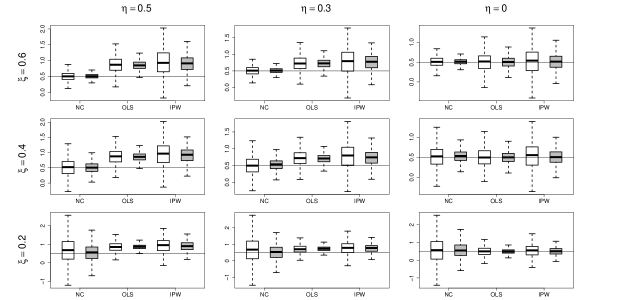
Figure 1: Boxplots for estimators of the average causal effect.

Note: For NC, $b=(1,X,V,W,XV,XW)\gamma$ and $q=(1,X,V,Z,XV,XZ)^{\rm T}$ are used for the GMM; for IPW, a logistic model for $\text{pr}(X=1\mid V)$ is used; for OLS, a linear model is used. White boxes are for sample size $500$ and gray ones $1500$; the horizontal line marks the true value of the average causal effect.

Table 1: Coverage probability of $95\%$ negative control confidence interval for the average causal effect

			$\eta=0.5$			$0.3$			$0$
$\xi=$	0.6		0.945	0.936		0.958	0.953		0.954	0.935
	$0.4$		0.958	0.957		0.968	0.955		0.964	0.956
	$0.2$		0.953	0.963		0.970	0.963		0.978	0.979

Note: For each setting of $\eta$, the first column is for sample size $500$ and the second $1500$.

7.2 Simulations for a structural model with a continuous exposure

We generate i.i.d. data according to

$$V,U\thicksim N(0,1),\quad\sigma_{uv}=0.5,\quad Z=0.5+1.5V+\eta U+\varepsilon_{1},$$

$$X=0.5+Z+0.5V+0.5V^{2}+1.5U+\varepsilon_{2},\quad W=1-V+\xi V^{2}+1.5U+\varepsilon_{3},$$

$$Y=1+0.5X+V+U+2\varepsilon_{3},\quad\varepsilon_{1},\varepsilon_{2},\varepsilon_{3}\thicksim N(0,1),$$

under multiple parameter settings: $\eta=0,0.3,0.5$ and $\xi=0,0.4,0.6$. We focus on the coefficient of $X$ in the outcome model. We analyze data with the negative control approach (NC), ordinary least square (OLS), and instrumental variable estimation (IV).

For each parameter setting, we replicate $1000$ simulations at sample size $500$ and $1500$, respectively. Figure 2 presents boxplots of three estimators. The negative control estimator has small bias whenever the confounding bridge is correctly specified ($\xi=0$). When the confounding bridge is incorrect ($\xi=0.4,0.6$), although the negative control estimator could be biased, the bias is much smaller than the other two estimators and reduces to zero as the association between $Z$ and $U$ becomes weak ($\eta=0,0.3$). This confirms the double robustness property of the proposed negative control estimator of Section 5. From Table 2, the $95\%$ negative control confidence intervals have coverage probability approximating $0.95$ if either the confounding bridge is correct or $Z$ is a valid instrumental variable. But when both conditions are violated, the coverage probability is below the nominal level. When $Z$ is a valid instrumental variable ($\eta=0$), the instrumental variable estimator also performs well with small bias, but is less efficient than the negative control estimator under the settings considered here, and can be severely biased when $Z$ and $U$ are correlated ($\eta=0.3,0.5$). The ordinary least square estimator is biased under all settings, due to confounding. Therefore, when a structural model is of interest, we recommend the negative control approach to reduce possible bias caused by confounding or an invalid instrumental variable.

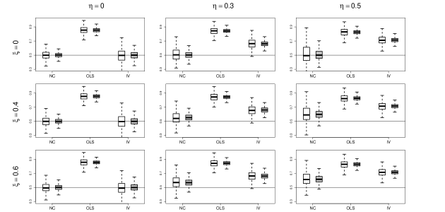
Figure 2: Boxplots for estimators of the structural parameter.

Note: For NC, $b=(1,X,V,W)\gamma$ and $q=(1,X,V,Z-\widehat{Z})^{\rm T}$ are used for the GMM with $\widehat{Z}$ obtained from a linear regression of $Z$ on $V$; for IV, two stage least square is used; for OLS, a linear model is used. White boxes are for sample size $500$ and gray ones $1500$; the horizontal line marks the true value of the parameter.

Table 2: Coverage probability of $95\%$ negative control confidence interval for the structural parameter

			$\eta=0$			$0.3$			$0.5$
$\xi=$	0		0.960	0.946		0.948	0.953		0.941	0.942
	$0.4$		0.956	0.942		0.971	0.855		0.964	0.712
	$0.6$		0.962	0.955		0.930	0.763		0.877	0.473

Note: For each setting of $\eta$, the first column is for sample size 500 and the second 1500.

7.3 Simulations for time series data

We generate data according to

$$U_{i}=\xi U_{i-1}+(1-\xi^{2})^{1/2}\varepsilon_{1i},\quad V_{i}=0.6U_{i}+\varepsilon_{2i},\quad X_{i}=0.4+1.5V_{i}+\eta U_{i}+\varepsilon_{3i},$$

$$Y_{i}=0.5+0.7X_{i}+1.5V_{i}+0.9U_{i}+\varepsilon_{4i},\quad\varepsilon_{1i},\varepsilon_{2i},\varepsilon_{3i},\varepsilon_{4i}\thicksim N(0,1),$$

where $U_{i}$ is a stationary autoregressive process with autocorrelation coefficient $\xi$, and $\eta$ controls the magnitude of confounding. We analyze data with the negative control approach (NC), ordinary least square (OLS) without controlling lagged exposures, and lagged-OLS by controlling one-day lagged exposure. For the negative control approach, we use $W_{i}=Y_{i-1}$ and $Z_{i}=X_{i+1}$ as negative controls, and do not need auxiliary data.

For each choice of $\xi=0.7,0.8,0.9$ and $\eta=0,0.3,0.5$, we replicate $1000$ simulations at sample size $500$ and $1500$, respectively. Figure 3 presents boxplots of the estimators. The negative control estimator has small bias in all nine scenarios, and its variability becomes smaller as autocorrelation of the confounder process increases. The $95\%$ negative control confidence intervals have coverage probability approximating $0.95$, as shown in Table 3. The ordinary least square estimator is biased except under no unmeasured confounding ($\eta=0$), in which case, it is more efficient than the negative control estimator. Controlling lagged exposures in ordinary least square can reduce confounding bias, but cannot eliminate it. Therefore, we recommend the negative control approach for estimation of a linear time-series regression model when unmeasured confounding may be present.

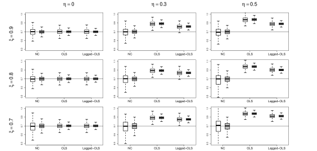
Figure 3: Boxplots for time series data analysis.

Note: For NC, $b=(1,X_{i},X_{i-1},V_{i},V_{i-1},W_{i})\gamma$ and $q=(1,X_{i},X_{i-1},V_{i},V_{i-1},Z_{i})^{\rm T}$ are used for the GMM. White boxes are for sample size $500$ and gray ones $1500$; the horizontal line marks the true value of the structural parameter.

Table 3: Coverage probability of $95\%$ negative control confidence interval for the time-series model

			$\eta=0$			$0.3$			$0.5$
$\xi=$	$0.9$		0.953	0.947		0.948	0.950		0.950	0.947
	$0.8$		0.979	0.952		0.952	0.943		0.933	0.946
	$0.7$		0.982	0.974		0.937	0.942		0.912	0.940

Note: For each setting of $\eta$, the first column is for sample size $500$ and the second $1500$. Confidence intervals are obtained from a normal approximation and the Newey & West (1987) variance estimator is used.

8 Evaluation of the effect of air pollution on mortality

While there are many long-term threats posed by air pollution, its acute effects on mortality also pose an important public health concern. We apply the negative control approach to evaluate the short-term effect of air pollution on mortality using datasets from a time-series study in Philadelphia, New York, and Boston. Here we present the analysis results for Philadelphia and relegate those for the other two cities to the Supplementary Materials. The dataset for Philadelphia contains $2621$ daily records of PM2.5, temperature, ozone, date, and number of deaths in Philadelphia from 1999 to 2006. With accidental deaths excluded, the number of deaths ranges from 73 to 179, which is often assumed to have a Poisson distribution. In our analysis, we use square root of the number of deaths for the purpose of normalization and variance stabilization (Freeman & Tukey, 1950).

For a given day $i$, we let $Y_{i}$ denote the square root of number of deaths, $X_{i}$ be the PM2.5 concentration measurement, $V_{i}$ consist of temperature and its square, ozone, and $X_{i-1}$ to control lagged effects, and $T_{i}$ consist of polynomial and Fourier bases of time to account for both secular and seasonal trends:

$$T_{i}=\{i/n,i^{2}/n^{2},\sin(2\pi i/365),\cos(2\pi i/365),\ldots,\sin(8\pi i/365),\cos(8\pi i/365)\},\quad n=2621.$$

We assume a linear outcome model, $Y_{i}=\beta_{1}X_{i}+(1,V_{i},T_{i})\beta_{2}+U_{i}$, and we are interested in the regression coefficient $\beta_{1}$ that encodes the immediate effect of current day PM2.5 on mortality. All results are summarized in Table 4. A standard regression analysis shows that short-term exposure to PM2.5 can significantly increase mortality, with point estimate $0.0084$ and $95\%$ confidence interval $(0.0048,0.0120)$ for $\beta_{1}$. However, a confounding test by fitting the model

$$W_{i}=\alpha_{1}X_{i}+\alpha_{2}Z_{i}+(1,X_{i-1},V_{i-1},T_{i-1})\alpha_{3}+U_{i-1},$$

with $W_{i}=Y_{i-1}$, results in point estimate $-0.0040$ of $\alpha_{1}$ with $95\%$ confidence interval $(-0.0073,-0.0007)$ and p-value $0.0167$, and point estimate $0.0041$ of $\alpha_{2}$ with $95\%$ confidence interval $(0.0011,0.0071)$ and p-value $0.0072$. These results suggest presence of unmeasured confounding because $W_{i}$ occurs before $X_{i}$ and $Z_{i}$, and should not be affected by them. Thus, ordinary least square appears not entirely appropriate in this setting. We apply the proposed negative control approach and use $Z_{i}=X_{i+1}$ and $W_{i}=Y_{i-1}$ as the negative control exposure and outcome, respectively. We assume a linear confounding bridge $b=(1,X_{i},V_{i},V_{i-1},T_{i},W_{i})\beta$, and use $q=(1,X_{i},V_{i},V_{i-1},T_{i},Z_{i})^{\rm T}$ for the GMM. Compared to the standard regression, the negative control estimate of $\beta_{1}$ is attenuated toward zero a lot, although it still has some significance with point estimate $0.0045$ and $95\%$ confidence interval $(-0.0006,0.0097)$. Further analyses controlling longer lagged exposures by including $X_{i-2}$ and $X_{i-3}$ in $V_{i}$ lead to analogous results as those obtained when only $X_{i-1}$ is controlled. Our analyses indicate presence of unmeasured confounding in the air pollution study in Philadelphia. In parallel analyses we provide in the Supplemental Materials, unmeasured confounding is also detected in the dataset for New York via the negative control approach, but not detected in the dataset for Boston. After accounting for unmeasured confounding, our negative control inference shows a significant acute effect of PM2.5 on mortality in Philadelphia, but such an effect is not detected in New York or Boston.

Table 4: Estimates of the effect of air pollution in Philadelphia

		Number of lagged exposures controlled
		One day			Two days			Three days
		Estimate	p-value		Estimate	p-value		Estimate	p-value
Ordinary least square
$\beta_{1}$		84 (48, 120)	0		78 (41, 115)	0		79 (43, 116)	0
Confounding test
$\alpha_{1}$		-40 (-73, -7)	0.0167		-39 (-71, -7)	0.0174		-40 (-72, -7)	0.0158
$\alpha_{2}$		41 (11, 71)	0.0072		40 (10, 69)	0.0080		39 (10, 69)	0.0083
Negative control estimation
$\beta_{1}$		45 (-6, 97)	0.0854		46 (-6, 98)	0.0844		46 (-7, 99)	0.0915

Note: Point estimates and $95\%$ confidence intervals (in brackets) in the table are multiplied by 10000. Confidence intervals and p-values are obtained from a normal approximation and the Newey & West (1987) variance estimator is used to account for serial correlation.

9 Discussion

We propose a confounding bridge approach for negative control inference on causal effects. We clarify the key assumptions and the roles of negative control outcome and exposure, and discuss robustness and sensitivity of the approach. Our approach enjoys the ease of implementation of standard parametric inference methods such as the GMM and two stage least square. Sometimes, it is of interest to consider a semiparametric or nonparametric confounding bridge, in which case, semiparametric methods such as sieve estimation (Ai & Chen, 2003) can be applied. We establish the connection between the negative control approach and the influential instrumental variable approach. Under a linear structural model, we show double robustness property of the negative control estimator, a property known to hold in certain causal inference problems (Robins et al., 1994; Van der Laan & Robins, 2003; Bang & Robins, 2005; Tchetgen Tchetgen et al., 2010).

Besides for causal effect evaluation, our approach has important implications for the design of observational studies. Even if an exposure or response factor is not relevant to the study in view, it is useful to collect them and use them as negative controls for the purpose of confounding diagnostic and bias adjustment. Time-series studies, such as the air pollution example we consider, are particularly well-suited for the proposed negative control approach, because negative controls can be constructed from observations of the exposure and outcome themselves; however in general, our approach requires one to collect extra data about negative control variables. For the instrumental variable design, we recommend that one collects negative control outcomes to enhance robustness of IV estimation.

The negative control assumptions we present in this paper describe the general principles for selecting negative control variables, and the examples we give provide guidance for certain specific studies; but in general, subject matter knowledge about the data generating mechanism and the potentially unmeasured confounders, such as specificity of the exposure-outcome relation (Hill, 1965; Lipsitch et al., 2010), is indispensable to choose an appropriate negative control.

Our approach has promising application in modern big and multi-source data analyses. Identification of the confounding bridge and the average causal effect depends only on $\text{pr}(Y,Z,X)$ and $\text{pr}(W,Z,X)$ but not the joint distribution of $(Y,W)$, and thus enjoys the convenience of data integration and two-sample inference. For certain confounding bridge models such as the linear one, estimation of the average causal effect requires only summary but not individual-level data, and thus allows for synthetic analysis by using results from multiple studies. Such extensions will be carefully developed in the future.

Supplementary Materials

Supplementary Materials include proofs of Propositions 1–2 and Theorems 1–3, details for examples and the GMM estimation, and analysis results for the effect of air pollution in New York and Boston.

Online Supplement to “A Confounding Bridge Approach for Double Negative Control Inference on Causal Effects”

This supplement includes proofs of Propositions 1–2 and Theorems 1–3, details for examples and the GMM estimation, and analysis results for the effect of air pollution in New York and Boston.

A Proofs of Propositions and Theorems

Proof of Propositions 1 and 2.

Given the confounding bridge assumption 3, we take expectation over $U$ on both sides of (2) and obtain that for all $x$,

$$E\{E(Y\mid U,X=x)\}=E\{E(b(W,x)\mid U,X=x)\}.$$

Under the latent ignorability assumption 1, we have $E\{E(Y\mid U,X=x)\}=E\{E(Y(x)\mid U)\}=E\{Y(x)\}$.

1. Under the negative control outcome assumption 2, we have $E\{E(b(W,x)\mid U,X=x)\}=E\{E(b(W,x)\mid U)\}=E\{b(W,x)\}$. Therefore, under Assumptions 1–3, we have $E\{Y(x)\}=E\{b(W,x)\}$, completing the proof of Proposition 1.

2. Under the positive control outcome assumption 7, we have $E\{E(b(W,x)\mid U,X=x)\}=E\{E(b(W(x),x)\mid U)\}=E\{b(W(x),x)\}$. Therefore, under Assumptions 1, 3, and 7, we have $E\{Y(x)\}=E\{b(W(x),x)\}$, completing the proof of Proposition 2.

∎

Proof of Theorems 1 and 2.

Proposition 1 implies that under Assumptions 1–3, for all $x$

$$E\{Y(x)\}=E\{b(W,x)\},$$ (S.1)

which establishes the relationship between the potential outcome mean and the negative control outcome distribution via the confounding bridge. Under Assumptions 2–4, we have that for all $x$,

$$E(Y\mid Z,X=x) = E\{E(Y\mid U,Z,X=x)\mid Z,X=x\}$$

$$= E\{E(Y\mid U,X=x)\mid Z,X=x\}$$

$$= E\{E(b(W,x)\mid U,X=x)\mid Z,X=x\}$$

$$= E\{E(b(W,x)\mid U,Z,X=x)\mid Z,X=x\}$$

$$= E\{b(W,x)\mid Z,X=x\},$$

where the first and fifth equalities are due to the law of iterated expectation, the second and forth are obtained due to the negative control exposure assumption 4, and the third is implied by the confounding bridge assumption 3. Therefore, we have that for all $x$,

$$E\{Y-b(W,x)\mid Z,X=x\}=0.$$ (S.2)

1. If there is no parametric or semiparametric restrictions imposed on the confounding bridge $b(W,X)$, we need completeness of $\text{pr}(W\mid Z,X)$ for identification of $b(W,X)$. Given Assumption 5, we show uniqueness of the solution to (S.2). Suppose both $b(W,X)$ and $b^{\prime}(W,X)$ satisfy (S.2), then we must have that for all $x$ and almost all $z$,

   $$E\{b(W,x)-b^{\prime}(W,x)\mid Z=z,X=x\}=0.$$

   However, Assumption 5 implies that for all $x$, $b(W,x)$ must equal $b^{\prime}(W,x)$ almost surely. Thus, the solution to (S.2) is unique, and therefore, the results of Theorem 1 hold, i.e., under Assumptions 1–5, the confounding bridge $b(W,X)$ is identified from (S.2), and the potential outcome mean is identified by (S.1).

2. If a parametric or semiparametric model $b(W,X;\gamma)$ is specified for the confounding bridge with a finite or infinite dimensional parameter $\gamma$, we only need a weakened version of completeness. Suppose that both $b(W,X;\gamma)$ and $b(W,X;\gamma^{\prime})$ satisfy (S.2) but $\gamma\neq\gamma^{\prime}$, then we must have that for all $x$ and almost all $z$, $E\{b(W,x;\gamma)-b^{\prime}(W,x;\gamma^{\prime})\mid Z=z,X=x\}=0$, which leads to a contradiction with the condition in Theorem 2. Therefore, given Assumptions 1–4 and the weakened completeness condition of Theorem 2, the confounding bridge is identified and so is the potential outcome mean.

∎

Proof of Theorem 3.

We maintain the following regularity condition for Theorem 3,

$$\left(\begin{array}[]{cc}\widehat{\sigma}_{xx}&\widehat{\sigma}_{xw}\\ \widehat{\sigma}_{xz}&\widehat{\sigma}_{zw}\end{array}\right)\rightarrow\left(\begin{array}[]{cc}\sigma_{xx}&\sigma_{xw}\\ \sigma_{xz}&\sigma_{zw}\\ \end{array}\right)\text{ in probability,}$$ (S.7)

which states consistency of the empirical cross-covariance matrix between $(X,Z)$ and $(X,W)$.

Given that $E(Y\mid U,X)=\beta X+U$, $Z\text{ }\begin{picture}(9.0,8.0)\put(0.0,0.0){\line(1,0){9.0}} \put(3.0,0.0){\line(0,1){8.0}} \put(6.0,0.0){\line(0,1){8.0}} \end{picture}\text{ }Y\mid(U,X)$, $W\text{ }\begin{picture}(9.0,8.0)\put(0.0,0.0){\line(1,0){9.0}} \put(3.0,0.0){\line(0,1){8.0}} \put(6.0,0.0){\line(0,1){8.0}} \end{picture}\text{ }(Z,X)\mid U$, then $W$ is a negative control outcome for $X$ and $Z$ is a negative control exposure for $W$ and $Y$. We apply the GMM with $b(W,X;\gamma)=\gamma_{0}+\gamma_{1}X+\gamma_{2}W$, $q(X,Z)=(1,X,Z)^{\rm T}$, and $\Omega$ the identity weight matrix. It is equivalent to solving

$$\frac{1}{n}\sum_{i=1}^{n}(1,X_{i},Z_{i})^{\rm T}\{Y_{i}-(1,X_{i},W_{i})\gamma\}=0,$$ (S.8)

and leads to the GMM estimator

$$\widehat{\gamma}=\left\{\frac{1}{n}\sum_{i=1}^{n}\left(\begin{array}[]{ccc}1&X_{i}&W_{i}\\ X_{i}&X_{i}^{2}&X_{i}W_{i}\\ Z_{i}&X_{i}Z_{i}&Z_{i}W_{i}\end{array}\right)\right\}^{-1}\left\{\frac{1}{n}\sum_{i=1}^{n}\left(\begin{array}[]{c}Y_{i}\\ X_{i}Y_{i}\\ Z_{i}Y_{i}\end{array}\right)\right\}.$$

After some algebra, the second component of $\widehat{\gamma}$ can be represented as

$$\widehat{\gamma}_{1}=\frac{\widehat{\sigma}_{xw}\widehat{\sigma}_{zy}-\widehat{\sigma}_{xy}\widehat{\sigma}_{zw}}{\widehat{\sigma}_{xw}\widehat{\sigma}_{xz}-\widehat{\sigma}_{xx}\widehat{\sigma}_{zw}}.$$

Assuming the regularity condition (S.7) and $\sigma_{xw}\sigma_{xz}-\sigma_{xx}\sigma_{zw}\neq 0$, then $\widehat{\gamma}_{1}$ converges in probability to

$$\frac{\sigma_{xw}\sigma_{zy}-\sigma_{xy}\sigma_{zw}}{\sigma_{xw}\sigma_{xz}-\sigma_{xx}\sigma_{zw}}.$$ (S.9)

1. If $b(W,X;\gamma)$ is correct so that $E(Y\mid U,X)=E\{b(W,X;\gamma)\mid U,X\}=E\{\gamma_{0}+\gamma_{1}X+\gamma_{2}W\mid U,X\}$, ’ then we have $\gamma_{1}=\beta$ and $E(W\mid U)=(-\gamma_{0}+U)/\gamma_{2}$. Thus, we have $\sigma_{zy}=\beta\sigma_{xz}+\sigma_{zu}$, $\sigma_{zw}=1/\gamma_{2}\sigma_{zu}$, $\sigma_{xw}=1/\gamma_{2}\sigma_{xu}$, and $\sigma_{xy}=\beta\sigma_{xx}+\sigma_{xu}$; by such substitution, the quantity in (S.9) is in fact equal to $\beta$. Therefore, $\widehat{\gamma}_{1}$ converge in probability to $\beta$.

2. Given that $W\text{ }\begin{picture}(9.0,8.0)\put(0.0,0.0){\line(1,0){9.0}} \put(3.0,0.0){\line(0,1){8.0}} \put(6.0,0.0){\line(0,1){8.0}} \end{picture}\text{ }(Z,X)\mid U$, if $Z\text{ }\begin{picture}(9.0,8.0)\put(0.0,0.0){\line(1,0){9.0}} \put(3.0,0.0){\line(0,1){8.0}} \put(6.0,0.0){\line(0,1){8.0}} \end{picture}\text{ }U$ and $\sigma_{xz}\neq 0$, i.e., $Z$ is a valid instrumental variable, then we have $\sigma_{zw}=0$. As a result, the quantity in (S.9) is equal to $\sigma_{zy}/\sigma_{xz}$, and thus equal to $\beta$. Therefore, $\widehat{\gamma}_{1}\rightarrow\beta$ in probability.

In summary, $\widehat{\gamma}_{1}$ is consistent if either condition (i) or (ii) of Theorem 3 holds, but not necessarily both. ∎

Equivalence to two stage least square. Solving (S.8) is equivalent to solving

$$\frac{1}{n}\sum_{i=1}^{n}(1,X_{i},Z_{i})^{\rm T}\{Y_{i}-(1,X_{i},\widehat{W}_{i})\gamma+\gamma_{2}(\widehat{W}_{i}-W_{i})\}=0,$$ (S.10)

with $\widehat{W}=(1,X,Z)\widehat{\alpha}$ and $\widehat{\alpha}$ solving the first stage least square,

$$\frac{1}{n}\sum_{i=1}^{n}(1,X_{i},Z_{i})^{\rm T}\{W-(1,X,Z)\alpha\}=0.$$

In particular, the coefficient of $Z$ obtained in the first stage least square is

$$\frac{\widehat{\sigma}_{xw}\widehat{\sigma}_{xz}-\widehat{\sigma}_{xx}\widehat{\sigma}_{zw}}{\widehat{\sigma}_{xz}^{2}-\widehat{\sigma}_{xx}\widehat{\sigma}_{zz}},$$

which can be used to test how far away the denominator in (S.9) is from zero. As a result, (S.8) is equivalent to

$$\frac{1}{n}\sum_{i=1}^{n}(1,X_{i},Z_{i})^{\rm T}\{Y_{i}-(1,X_{i},\widehat{W}_{i})\gamma\}=0,$$

and also equivalent to

$$\frac{1}{n}\sum_{i=1}^{n}(1,X_{i},\widehat{W}_{i})^{\rm T}\{Y_{i}-(1,X_{i},\widehat{W}_{i})\gamma\}=0,$$

because $\widehat{W}_{i}$ is a linear combination of $X_{i}$ and $Z_{i}$. Therefore, the negative control estimator $\widehat{\beta}_{\rm nc}$ is equivalent to the two stage least square estimator.

B Details for Examples

Details for Example 3. Consider the data generating process of Example 3 and the following two parameter settings.

Table 5: Two distinct parameter settings with identical observed data distribution

$\beta$	$\alpha_{1}$	$\alpha_{2}$	$\alpha_{3}$	$\sigma_{1}^{2}$	$\sigma_{2}^{2}$	$\sigma_{3}^{2}$
1	1	1	1	1	1	4
-1	$\sqrt{3/5}$	$\sqrt{5/3}$	$\sqrt{15}$	$7/5$	$1/3$	2

These two parameter settings with distinct values of $\beta$ result in identical distribution of $(X,Y,W)$, which is a joint normal distribution with mean zero and covariance matrix:

$$\left(\begin{array}[]{ccc}2&3&1\\ 3&9&2\\ 1&2&2\end{array}\right).$$

Therefore, given the distribution of $(X,Y,W)$, $\beta$ encoding the average causal effect is not identified.

Details for Example 8. We first describe a general result for the relationship between the average causal effect and crude effects. For a confounding bridge function $b(W,X)$, because $E\{Y(x)\}=E\{b(W,x)\}$ and $E\{Y\mid Z,X\}=E\{b(W,X)\mid Z,X\}$, we have that for any two values $x_{1},x_{0}$ in the support of $X$,

$$E\{Y(x_{1})\}-E\{Y(x_{0})\}$$

$$= \int_{w}b(w,x_{1})\text{pr}(w)dw-\int_{w}b(w,x_{0})\text{pr}(w)dw$$

$$= \int_{w,x,z}b(w,x_{1})\text{pr}(w\mid z,x)\text{pr}(z,x)dzdxdw-\int_{w,x,z}b(w,x_{0})\text{pr}(w\mid z,x)\text{pr}(z,x)dzdxdw$$

$$= \int_{w,x,z}b(w,x_{1})\text{pr}(w\mid z,x_{1})\text{pr}(z,x)dzdxdw-\int_{w,x,z}b(w,x_{0})\text{pr}(w\mid z,x_{0})\text{pr}(z,x)dzdxdw$$

$$-\int_{w,x,z}b(w,x_{1})\{\text{pr}(w\mid z,x_{1})-\text{pr}(w\mid z,x_{0})\}\text{pr}(z,x)dzdxdw$$

$$+\int_{w,x,z}\{b(w,x_{1})-b(w,x_{0})\}\{\text{pr}(w\mid z,x)-\text{pr}(w\mid z,x_{0})\}\text{pr}(z,x)dzdxdw$$

$$= E\{E(Y\mid Z,x_{1})-E(Y\mid Z,x_{0})\}$$

$$-\int_{w,z}b(w,x_{1})\{\text{pr}(w\mid z,x_{1})-\text{pr}(w\mid z,x_{0})\}\text{pr}(z)dzdw$$

$$+\int_{w,x,z}\{b(w,x_{1})-b(w,x_{0})\}\{\text{pr}(w\mid z,x)-\text{pr}(w\mid z,x_{0})\}\text{pr}(z,x)dzdxdw.$$

If the confounding bridge has the form $b(W,X)=b_{1}(X)+b_{2}(X)b_{0}(W)$, the last equality reduces to

$$E\{Y(x_{1})\}-E\{Y(x_{0})\} = E\{E(Y\mid Z,x_{1})-E(Y\mid Z,x_{0})\}$$

$$-b_{2}(x_{1})E\{E(b_{0}(W)\mid Z,x_{1})-E(b_{0}(W)\mid Z,x_{0})\}$$

$$+\{b_{2}(x_{1})-b_{2}(x_{0})\}\int_{x,z}\{E(b_{0}(W)\mid Z=z,x)-E(b_{0}(W)\mid Z=z,x_{0})\}\text{pr}(z,x)dzdx.$$

Next, we consider the setting of Example 8 with binary $(X,Z)$ and $b(W,X;\gamma)=\gamma_{0}+\gamma_{1}X+\gamma_{2}W+\gamma_{3}XW$, in which case, $b_{1}(X)=\gamma_{0}+\gamma_{1}X$, $b_{2}(X)=\gamma_{2}+\gamma_{3}X$, $b_{0}(W)=W$. Then we obtain that

$$E\{Y(1)\}-E\{Y(0)\} = E\{E(Y\mid Z,X=1)-E(Y\mid Z,X=0)\}$$

$$-(\gamma_{2}+\gamma_{3})E\{E(W\mid Z,X=1)-E(W\mid Z,X=0)\}$$

$$+\gamma_{3}\sum_{z=0}^{1}\{E(W\mid Z=z,X=1)-E(W\mid Z=z,X=0)\}\text{pr}(Z=z,X=1).$$

The unknown parameters $\gamma$ are identified by solving $E(Y\mid Z,X)=E\{b(W,X;\gamma)\mid Z,X\}$:

$$\gamma_{2}=\frac{E(Y\mid Z=1,X=0)-E(Y\mid Z=0,X=0)}{E(W\mid Z=1,X=0)-E(W\mid Z=0,X=0)},$$

$$\gamma_{2}+\gamma_{3}=\frac{E(Y\mid Z=1,X=1)-E(Y\mid Z=0,X=1)}{E(W\mid Z=1,X=1)-E(W\mid Z=0,X=1)}.$$

If $\gamma_{3}=0$, then

$$\gamma_{2}=\frac{E\{E(Y\mid Z=1,X)-E(Y\mid Z=0,X)\}}{E\{E(W\mid Z=1,X)-E(W\mid Z=0,X)\}}.$$

C Details for estimation

Define the moment restrictions

$$h(D_{i};\theta)=\left\{\begin{array}[]{l}\{Y_{i}-b(W_{i},V_{i},X_{i};\gamma)\}\times q(X_{i},V_{i},Z_{i})\\ \Delta-\{b(W_{i},V_{i},x_{1};\gamma)-b(W_{i},V_{i},x_{0};\gamma)\}\end{array}\right\},$$ (S.13)

with a user-specified vector function $q$, and let $m_{n}(\theta)=1/n\sum_{i=1}^{n}h(D_{i};\theta)$; the GMM solves

$$\widehat{\theta}=\text{arg }\min\limits_{\theta}\ m_{n}^{\rm T}(\theta)\ \Omega\ m_{n}(\theta),$$

with a user-specified positive-definite weight matrix $\Omega$.

Under appropriate conditions, consistency and asymptotic normality of the GMM estimator have been established (Hansen, 1982; Hall, 2005):

$$n^{1/2}(\widehat{\theta}-\theta_{0})\rightarrow N(0,\Sigma_{1}\Sigma_{0}\Sigma_{1}^{\rm T}),$$

where $\theta_{0}$ denotes the true value of $\theta$, and

$$\Sigma_{1}=(M^{\rm T}\Omega M)^{-1}M^{\rm T}\Omega,\quad M=\lim_{n\rightarrow+\infty}\left.\frac{\partial m_{n}(\theta)}{\partial\theta^{\rm T}}\right|_{\theta=\theta_{0}},\quad\Sigma_{0}=\lim_{n\rightarrow+\infty}{\rm Var}\{n^{1/2}m_{n}(\theta_{0})\}.$$

For i.i.d. data, a consistent estimator of the asymptotic variance can be constructed by using

$$\widehat{\Sigma}_{1}=(\widehat{M}^{\rm T}\Omega\widehat{M})^{-1}\widehat{M}^{\rm T}\Omega,\quad\widehat{M}=\frac{1}{n}\sum_{i=1}^{n}\left.\frac{\partial h(D_{i};\theta)}{\partial\theta^{\rm T}}\right|_{\theta=\widehat{\theta}},\quad\widehat{\Sigma}_{0}=\frac{1}{n}\sum_{i=1}^{n}h(D_{i};\widehat{\theta})h^{\rm T}(D_{i};\widehat{\theta});$$ (S.14)

and a $95\%$ confidence interval for the elements of $\theta$ in large samples is $\widehat{\theta}\pm 1.96\times\{{\rm diag}(\widehat{\Sigma}_{1}\widehat{\Sigma}_{0}\widehat{\Sigma}_{1}^{\rm T})/n\}^{1/2}$, where diag denotes the diagonal elements of a matrix.

When the observe data are serially correlated, $\widehat{\Sigma}_{0}$ in (S.14) is no longer consistent for $\Sigma_{0}$, and one should use heteroscedasticity and autocorrelation covariance (HAC) estimators that are consistent under relatively weak assumptions (Newey & West, 1987; Andrews, 1991). In this paper, we use the Newey-West estimate of $\Sigma_{0}$:

$$\Sigma_{0}^{\rm HAC} = \widehat{\Sigma}_{0}+\sum_{i=1}^{b_{n}}\{1-\frac{i}{1+b_{n}}\}(\widehat{\Sigma}_{i}+\widehat{\Sigma}_{i}^{\rm T}),\quad b_{n}=c\times n^{1/3}{\text{ for some constant c}},$$

$$\widehat{\Sigma}_{i} = \frac{1}{n}\sum_{j=i+1}^{n}h(D_{j};\widehat{\theta})h^{\rm T}(D_{j-i};\widehat{\theta}),$$

where $b_{n}$ is the bandwidth parameter controlling the number of auto-covariances included in the HAC estimator; for practical guidance for the choice of $b_{n}$, see Andrews (1991) and Hall (2005, section 3.5.3). In contrast to the i.i.d. setting, the HAC estimator includes extra covariance terms $\{\widehat{\Sigma}_{i},i\neq 0\}$ to account for the serial correlation.

D Analysis results for Philadelphia and Boston

Table 6: Estimates of the effect of air pollution in New York

		Number of lagged exposures controlled
		One day			Two days			Three days
		Estimate	p-value		Estimate	p-value		Estimate	p-value
Ordinary least square
$\beta_{1}$		37 (1, 72)	0.0410		30 (-6, 66)	0.1016		32 (-3, 68)	0.0742
Confounding test
$\alpha_{1}$		-5 ( -39, 29)	0.7662		-3 (-36, 30)	0.8792		-1 (-33, 32)	0.9758
$\alpha_{2}$		25 (-7, 57)	0.1188		24 (-7, 54)	0.1327		24 (-7, 54)	0.1328
Negative control estimation
$\beta_{1}$		-8 (-43, 28)	0.6678		-7 (-45, 30)	0.7024		-7 (-46, 32)	0.7370

Table 7: Estimates of the effect of air pollution in Boston

		Number of lagged exposures controlled
		One day			Two days			Three days
		Estimate	p-value		Estimate	p-value		Estimate	p-value
Ordinary least square
$\beta_{1}$		1 (-37, 39)	0.9685		-3 (-42, 35)	0.8580		-5 (-43, 34)	0.8160
Confounding test
$\alpha_{1}$		10 (-28, 48)	0.6084		12 (-25, 49)	0.5222		12 (-25, 49)	0.5208
$\alpha_{2}$		-7 (-41, 27)	0.6758		-7 (-41, 27)	0.6945		-8 (-42, 26)	0.6596
Negative control estimation
$\beta_{1}$		-26 (-71, 19)	0.2643		-25 (-71, 21)	0.2813		-25 (-73, 23)	0.3064

Note for Tables 6 and 7: Point estimates and $95\%$ confidence intervals (in brackets) in the table are multiplied by 10000. Confidence intervals and p-values are obtained from a normal approximation and the Newey & West (1987) variance estimator is used to account for serial correlation.

Sample Codes
Instructions

This supplement contains R sample programs for negative control estimation in the time-series setting when confounding arises. Three R scripts are included: Timeseries_Simu.R, Timeseries_SimuFun.R, and BasGmmFun.R.

Timeseries_Simu.R is the main program for simulation, and requires the other two R scripts.

Timeseries_SimuFun.R includes a function simuTimeseries for data generation, model fitting, and parameter estimation. Data are generated from linear models, and GMM is used for negative control estimation of the structural parameter, and function NCmrf specifies the moment restriction used for GMM.

BasGmmFun.R includes supporting routines such as those for variance estimation. Note that, HAC estimator should be used in the time-series or serially correlated setting. More details and explanation are included in the programs.

A comprehensive and user–friendly package for negative control inference is under development.

Correspondence:

Wang Miao
Peking University
mwfy@pku.edu.cn

Listing 1: Timeseries_Simu.R

⬇

# By Wang Miao, Peking University, mwfy@pku.edu.cn

# Apr 12, 2018

# Sample colde for negative control estimation

# Simulation example for Timeseries data

# Coninuous exposure, continuous outcome

# Linear models, without seasonality

# rm(list=ls())

# set workdir before running

source(’BasGmmFun.R’)

source(’Timeseries_SimuFun.R’)

k <- 1; q <- 10;

vbeta <- 0.6; xi <- 0.8

xbeta <- c(0.4, 1.5, 0.3)

# 0.7 is the true value of the structural parameter

ybeta <- c(0.5, 0.7, 1.5, 0.9)

para <- list(k=k,q=q,xi=xi,vbeta=vbeta,xbeta=xbeta,ybeta=ybeta)

N <- 1500

# Initial value for optimization in GMM estimation

inioptim=c(-0.5, 0.7, -1, 1.5, -2, 1.5)

# One simulation

rslt <- simuTimeseries(para,N,inioptim)

nc <- rslt$nc; ols <- rslt$ols;

olslag <- rslt$olslag;

hacdvar <- rslt$hacdvar

0.7;#truth

nc;ols;olslag; #estimators

Listing 2: Timeseries_SimuFun.R

⬇

# By Wang Miao, Peking University, mwfy@pku.edu.cn

# Apr 12, 2018

# Sample colde for negative control estimation

# Simulation function for Timeseries data

# Coninuous exposure, continuous outcome

# Linear models, without seasonality

# Moment restriction function

NCmrf <- function(para,data1){

X <- as.matrix(data1$X); Y <- as.matrix(data1$Y)

Z <- as.matrix(data1$Z); W <- as.matrix(data1$W)

V <- as.matrix(data1$V)

hlink <- cbind(1,X,V,W) %*% para

g0 <- cbind(1,X,V,Z)

g <- (as.vector(Y - hlink)) * g0

return(g)

}

simuTimeseries <- function(para,N,inioptim){

# Parameters

## para includes the model parameters for data generation,

## N sample size

## inioptim the initial value for optimzation in GMM estimation

## X_i+k and Y_i-k are used as NCs

k <- para$k;

## bandwidth parameter for HAC estimator

q <- para$q;

vbeta <- para$vbeta; xi <- para$xi;

xbeta <- para$xbeta; ybeta <- para$ybeta

# Generate data

## the unobserved confounder, is AR(1) with parameter xi

U0 <- arima.sim(n=N, list(ar=xi), sd=sqrt(1 - xi^2))

## the observed confounder

V0 <- U0 * vbeta + rnorm(N,mean=0,sd=1)

## the exposure

X0 <- cbind(1,V0,U0) %*% xbeta + rnorm(N,mean=0,sd=1)

## the outcome, ybeta[2] is the structural parameter of interest

Y0 <- cbind(1,X0,V0,U0) %*% ybeta + rnorm(N,mean=0,sd=1)

# Estimation

## OLS with observed data

lmols <- lm(Y0~X0+V0)

ols <- as.numeric(lmols$coef[2])

## construct NCs from observed data

lnth <- length(Y0)

lnthW <- 1:(lnth-k-1)

lnthY <- (k+1):(lnth-1)

lnthZ <- (k+2):lnth

Y <- Y0[lnthY]; yX <- X0[lnthY]

W <- Y0[lnthW]; wX <- X0[lnthW]

Z <- X0[lnthZ]

yV <- V0[lnthY] # covariates associated with Y

wV <- V0[lnthW] # covariates associated with W

## data used for NC estimation

data1 <- list(X=yX,Y=Y,Z=Z,W=W,V=cbind(wX,yV,wV))

# GMM for NC estimation

hpar <- optim(par = inioptim,

fn = GMMF,

mrf = NCmrf, data = data1,

method = "BFGS", hessian = FALSE)$par

# This is the NC estimator of the structural parameter

nc <- as.numeric(hpar[2])

# OLS with lags included

lmlag <- lm(Y ~ yX + wX + yV + wV + W)

olslag <- as.numeric(lmlag$coef[2])

# Variance estimation

var_est <- HAC_VAREST(NCmrf,hpar,q=q,data1)

dvar <- diag(var_est$var)

hacdvar <- diag(var_est$hacvar)

return(list(nc=nc,ols=ols,olslag=olslag,hacdvar=hacdvar,dvar=dvar))

}

Listing 3: BasGmmFun.R

⬇

# By Wang Miao, Peking University, mwfy@pku.edu.cn

# Apr18, 2018

# Basic functions GMM estimation and variance estimation

library(numDeriv)

# GMM function

GMMF <- function(mrf,para,data){

g0 <- mrf(para=para,data=data)

g <- apply(g0,2,mean)

gmmf <- sum(g^2)

return(gmmf)

}

# Derivative of score equations

G1 <- function(bfun,para,data){

G1 <- apply(bfun(para,data),2,mean)

return(G1)

}

G <- function(bfun,para,data){

G <- jacobian(func=G1,bfun=bfun,x=para,data=data)

return(G)

}

# Variance estimation

VAREST <- function(bfun,para,data){

bG <- solve(G(bfun,para,data))

bg <- bfun(para,data)

spsz <- dim(bg)[1]

Omega <- t(bg)%*%bg/spsz

Sigma <- bG%*%Omega%*%t(bG)

return(Sigma/spsz)

}

# Newey-West 1987 variance estimator for serially correlated data

HAC_VAREST <- function(bfun,para,q,data){

bG <- solve(G(bfun,para,data))

bg <- bfun(para,data)

spsz <- dim(bg)[1]

hacOmega <- Omega <- t(bg)%*%bg/spsz

for(i in 1:q){

Omega_i <- t(bg[-(1:i),])%*%bg[1:(spsz-i),]/spsz

hacOmega <- hacOmega + (1 - i/(q+1))*(Omega_i + t(Omega_i))

}

Sigma <- bG%*%Omega%*%t(bG)

hacSigma <- bG%*%hacOmega%*%t(bG)

return(list(var=Sigma/spsz, hacvar=hacSigma/spsz))

}

# Confidence interval

CNFINTVl <- function(esti, ci){

esti <- as.matrix(esti)

dm <- dim(esti)[2]

para <- esti[,1:(dm/2)]

dvar <- esti[,(dm/2+1):dm]

z <- -qnorm((1-ci)/2)

dsd <- sqrt(dvar)

return(list(lb=para-z*dsd, ub=para+z*dsd))

}

# Coverage probability

CVRPRB <- function(esti,ci,trvlu){

esti <- as.matrix(esti)

dm <- dim(esti)[2]

para <- esti[,1:(dm/2)]

dvar <- esti[,(dm/2+1):dm]

z <- -qnorm((1-ci)/2)

dsd <- sqrt(dvar)

lb <- para-z*dsd; ub <- para+z*dsd

return(trvlu>=lb&trvlu<=ub)

}

# P-value based on normal approximation

PVALUE <- function(esti){

esti <- as.matrix(esti)

dm <- dim(esti)[2]

para <- esti[,1:(dm/2)]

dvar <- esti[,(dm/2+1):dm]

dsd <- sqrt(dvar)

return((1 - pnorm(abs(para),mean=0,sd=dsd))*2)

}

REFERENCES

- Ai & Chen (2003) Ai, C. & Chen, X. (2003). Efficient estimation of models with conditional moment restrictions containing unknown functions. Econometrica 71, 1795–1843.
- Andrews (1991) Andrews, D. W. (1991). Heteroskedasticity and autocorrelation consistent covariance matrix estimation. Econometrica 59, 817–858.
- Andrews (2017) Andrews, D. W. (2017). Examples of -complete and boundedly-complete distributions. Journal of Econometrics 199, 213–220.
- Angrist et al. (1996) Angrist, J., Imbens, G. & Rubin, D. (1996). Identification of causal effects using instrumental variables. Journal of the American Statistical Association 91, 444–455.
- Baker & Lindeman (1994) Baker, S. G. & Lindeman, K. S. (1994). The paired availability design: a proposal for evaluating epidural analgesia during labor. Statistics in Medicine 13, 2269–2278.
- Bang & Robins (2005) Bang, H. & Robins, J. M. (2005). Doubly robust estimation in missing data and causal inference models. Biometrics 61, 962–973.
- Berkson (1958) Berkson, J. (1958). Smoking and lung cancer: some observations on two recent reports. Journal of the American Statistical Association 53, 28–38.
- Cornfield et al. (1959) Cornfield, J., Haenszel, W., Hammond, E. C., Lilienfeld, A. M., Shimkin, M. B. & Wynder, E. L. (1959). Smoking and lung cancer: recent evidence and a discussion of some questions. Journal of the National Cancer Institute 22, 173–203.
- Darolles et al. (2011) Darolles, S., Fan, Y., Florens, J. P. & Renault, E. (2011). Nonparametric instrumental regression. Econometrica 79, 1541–1565.
- Davey Smith (2008) Davey Smith, G. (2008). Assessing intrauterine influences on offspring health outcomes: can epidemiological studies yield robust findings? Basic & Clinical Pharmacology & Toxicology 102, 245–256.
- Davey Smith (2012) Davey Smith, G. (2012). Negative control exposures in epidemiologic studies. Epidemiology 23, 350–351.
- D’Haultfœuille (2011) D’Haultfœuille, X. (2011). On the completeness condition in nonparametric instrumental problems. Econometric Theory 27, 460–471.
- Didelez & Sheehan (2007) Didelez, V. & Sheehan, N. (2007). Mendelian randomization as an instrumental variable approach to causal inference. Statistical Methods in Medical Research 16, 309–330.
- Flanders et al. (2011) Flanders, W. D., Klein, M., Darrow, L. A., Strickland, M. J., Sarnat, S. E., Sarnat, J. A., Waller, L. A., Winquist, A. & Tolbert, P. E. (2011). A method for detection of residual confounding in time-series and other observational studies. Epidemiology 22, 59–67.
- Flanders et al. (2017) Flanders, W. D., Strickland, M. J. & Klein, M. (2017). A new method for partial correction of residual confounding in time-series and other observational studies. American Journal of Epidemiology 185, 941–949.
- Freeman & Tukey (1950) Freeman, M. F. & Tukey, J. W. (1950). Transformations related to the angular and the square root. The Annals of Mathematical Statistics 21, 607–611.
- Gagnon-Bartsch et al. (2013) Gagnon-Bartsch, J., Jacob, L. & Speed, T. P. (2013). Removing unwanted variation from high dimensional data with negative controls. Technical Report 820, Dept. Statistics, Univ. California, Berkeley .
- Gagnon-Bartsch & Speed (2012) Gagnon-Bartsch, J. A. & Speed, T. P. (2012). Using control genes to correct for unwanted variation in microarray data. Biostatistics 13, 539–552.
- Goldberger (1972) Goldberger, A. S. (1972). Structural equation methods in the social sciences. Econometrica 40, 979–1001.
- Hall (2005) Hall, A. R. (2005). Generalized Method of Moments. Oxford: Oxford University Press.
- Hamilton (1994) Hamilton, J. D. (1994). Time Series Analysis. Princeton: Princeton University Press.
- Hansen (1982) Hansen, L. P. (1982). Large sample properties of generalized method of moments estimators. Econometrica 50, 1029–1054.
- Hill (1965) Hill, A. B. (1965). The environment and disease: association or causation? Proceedings of the Royal Society of Medicine 58, 295.
- Hu & Shiu (2018) Hu, Y. & Shiu, J.-L. (2018). Nonparametric identification using instrumental variables: Sufficient conditions for completeness. Econometric Theory 34, 659–693.
- Khush et al. (2013) Khush, R. S., Arnold, B. F., Srikanth, P., Sudharsanam, S., Ramaswamy, P., Durairaj, N., London, A. G., Ramaprabha, P., Rajkumar, P., Balakrishnan, K. et al. (2013). H2S as an indicator of water supply vulnerability and health risk in low-resource settings: a prospective cohort study. The American Journal of Tropical Medicine and Hygiene 89, 251–259.
- Kuroki & Pearl (2014) Kuroki, M. & Pearl, J. (2014). Measurement bias and effect restoration in causal inference. Biometrika 101, 423–437.
- Lipsitch et al. (2010) Lipsitch, M., Tchetgen Tchetgen, E. & Cohen, T. (2010). Negative controls: A tool for detecting confounding and bias in observational studies. Epidemiology 21, 383–388.
- Mamun et al. (2006) Mamun, A. A., Lawlor, D. A., Alati, R., O’callaghan, M. J., Williams, G. M. & Najman, J. M. (2006). Does maternal smoking during pregnancy have a direct effect on future offspring obesity? Evidence from a prospective birth cohort study. American Journal of Epidemiology 164, 317–325.
- Miao et al. (2018) Miao, W., Geng, Z. & Tchetgen Tchetgen, E. (2018). Identifying causal effects with proxy variables of an unmeasured confounder. Biometrika , To appear.
- Miao & Tchetgen Tchetgen (2017) Miao, W. & Tchetgen Tchetgen, E. (2017). Invited commentary: Bias attenuation and identification of causal effects with multiple negative controls. American Journal of Epidemiology 185, 950–953.
- Newey & Powell (2003) Newey, W. K. & Powell, J. L. (2003). Instrumental variable estimation of nonparametric models. Econometrica 71, 1565–1578.
- Newey & West (1987) Newey, W. K. & West, K. D. (1987). A simple, positive semi-definite, heteroskedasticity and autocorrelation consistent covariance matrix. Econometrica 55, 703–708.
- Ogburn & VanderWeele (2013) Ogburn, E. L. & VanderWeele, T. J. (2013). Bias attenuation results for nondifferentially mismeasured ordinal and coarsened confounders. Biometrika 100, 241–248.
- Robins (1994) Robins, J. M. (1994). Correcting for non-compliance in randomized trials using structural nested mean models. Communications in Statistics-Theory and Methods 23, 2379–2412.
- Robins et al. (1994) Robins, J. M., Rotnitzky, A. & Zhao, L. P. (1994). Estimation of regression coefficients when some regressors are not always observed. Journal of the American Statistical Association 89, 846–866.
- Rosenbaum (1989) Rosenbaum, P. R. (1989). The role of known effects in observational studies. Biometrics 45, 557–569.
- Rosenbaum & Rubin (1983a) Rosenbaum, P. R. & Rubin, D. B. (1983a). Assessing sensitivity to an unobserved binary covariate in an observational study with binary outcome. Journal of the Royal Statistical Society. Series B 45, 212–218.
- Rosenbaum & Rubin (1983b) Rosenbaum, P. R. & Rubin, D. B. (1983b). The central role of the propensity score in observational studies for causal effects. Biometrika 70, 41–55.
- Rubin (1973) Rubin, D. B. (1973). The use of matched sampling and regression adjustment to remove bias in observational studies. Biometrics 29, 185–203.
- Schuemie et al. (2014) Schuemie, M. J., Ryan, P. B., DuMouchel, W., Suchard, M. A. & Madigan, D. (2014). Interpreting observational studies: why empirical calibration is needed to correct p-values. Statistics in Medicine 33, 209–218.
- Sofer et al. (2016) Sofer, T., Richardson, D. B., Colicino, E., Schwartz, J. & Tchetgen Tchetgen, E. J. (2016). On negative outcome control of unobserved confounding as a generalization of difference-in-differences. Statistical Science 31, 348–361.
- Stuart (2010) Stuart, E. A. (2010). Matching methods for causal inference: A review and a look forward. Statistical Science 25, 1–21.
- Tchetgen Tchetgen (2014) Tchetgen Tchetgen, E. (2014). The control outcome calibration approach for causal inference with unobserved confounding. American Journal of Epidemiology 179, 633–640.
- Tchetgen Tchetgen et al. (2010) Tchetgen Tchetgen, E. J., Robins, J. M. & Rotnitzky, A. (2010). On doubly robust estimation in a semiparametric odds ratio model. Biometrika 97, 171–180.
- Trichopoulos et al. (1983) Trichopoulos, D., Zavitsanos, X., Katsouyanni, K., Tzonou, A. & Dalla-Vorgia, P. (1983). Psychological stress and fatal heart attack: The athens (1981) earthquake natural experiment. The Lancet 321, 441–444.
- Van der Laan & Robins (2003) Van der Laan, M. J. & Robins, J. M. (2003). Unified Methods for Censored Longitudinal Data and Causality. New York: Springer.
- Wang et al. (2017) Wang, J., Zhao, Q., Hastie, T. & Owen, A. B. (2017). Confounder adjustment in multiple hypothesis testing. The Annals of Statistics 45, 1863–1894.
- Weiss (2002) Weiss, N. S. (2002). Can the “specificity” of an association be rehabilitated as a basis for supporting a causal hypothesis? Epidemiology 13, 6–8.
- Wooldridge (2010) Wooldridge, J. M. (2010). Econometric Analysis of Cross Section and Panel Data. MIT press: Cambridge.
- Wright (1928) Wright, P. G. (1928). Tariff on Animal and Vegetable Oils. New York: Macmillan.
- Yerushalmy & Palmer (1959) Yerushalmy, J. & Palmer, C. E. (1959). On the methodology of investigations of etiologic factors in chronic diseases. Journal of Chronic Diseases 10, 27–40.