Polyfold and SFT Notes II:
Local-Local M-Polyfold Constructions

These notes are the beginning chapters from the upcoming book [18]

J. W. Fish and H. Hofer,
Polyfold Constructions: Tools, Techniques, and Functors

which we make available for the upcoming workshop

Introduction

We aim to use polyfold theory to develop a a Fredholm Theory for SFT we need to construct so-called M-polyfolds and strong bundles over them. These arise as ambient spaces for a nonlinear Fredholm theory in the polyfold context. The relevant global M-polyfolds are build using a “LEGO”-type system, [50], from smaller building blocks. The construction of the “LEGO”-pieces is described in the local-local theory, which is the subject of the current paper.

In a follow up paper we shall show how these pieces can be plugged together (fibered product constructions) to carry out more complex constructions. This will rely on the abstract theory contained in the first part of this series,

J. W. Fish and H. Hofer, Polyfold and SFT Notes I:
A Primer on Polyfolds and Construction tools.

There we have provided an abstract theory which guarantees that local-local constructions, satisfying some properties, can be plugged together to produce local spaces with desired properties, i.e. a theory which guides the passage from the local-local to the local theory. This setup allows to recycle analysis in a controllable (i.e. checkable) fashion and to add novel construction which then automatically work with the other ingredients. A global theory is obtained from interacting local pieces. This will be described in the next paper.

We first recall some concrete sc-smoothness results from the paper [38]. This paper contains a plethora of results useful in concrete constructions. After this we shall study the situation of maps defined on a nodal Riemann surface as well as on the family of varying cylinders obtained by gluing. This is done in Section 2. We refer to this as the nodal construction. In Section 3 a similar construction is carried out in the context where we also have a periodic orbit. More precisely we construct a M-polyfold structure describing how maps defined on finite cylinders decompose in the presence of periodic orbits when the cylinders get infinitely long and approaches a nodal disk pair, while its image tries to approximate a cylinder over a periodic orbit. This will be referred to as the stretching near a periodic orbit construction. In Section 4 we summarize some classical constructions.

1. Sc-Smoothness Results

The following discussion follows closely some of the topics in [38].

1.1. Smoothness Versus Sc-Smoothness

It is important to know the relationship between the concepts of classical smoothness and sc-smoothness. The proofs of the following results can be found in [38]. The first theorem gives implicitly an alternative definition of sc-smoothness.

Theorem 1.1 (Proposition 2.1, [38]).

Let $U$ be a relatively open subset of a partial quadrant in a sc-Banach space $E$ and let $F$ be another sc-Banach space. Then a $\text{sc}^{0}$-map $f\colon U\to F$ is of class $\text{sc}^{1}$ if and only if the following conditions hold true.

• For every $m\geq 1$, the induced map $f\colon U_{m}\to F_{m-1}$ is of class $C^{1}$. In particular, the derivative

  $$df\colon U_{m}\to\mathscr{L}(E_{m},F_{m-1}),\quad x\mapsto df(x)$$

  is a continuous map.

• For every $m\geq 1$ and every $x\in U_{m}$, the bounded linear operator $df(x)\colon E_{m}\to F_{m-1}$ has an extension to a bounded linear operator $Df(x)\colon E_{m-1}\to F_{m-1}$. In addition, the map

  $$U_{m}\oplus E_{m-1}\to F_{m-1},\quad(x,h)\mapsto Df(x)h$$

  is continuous.

Remark 1.2.

If $x\in U_{\infty}$ is a smooth point in $U$ and $f\colon U\to F$ is a $\text{sc}^{1}$-map, then the linearization

$$Df(x)\colon E\to F$$

is a sc-operator.

A consequence of Theorem 1.1 is the following result about lifting the indices.

Proposition 1.3 (Proposition 2.2, [38]).

Let $U$ and $V$ be relatively open subsets of partial quadrants in sc-Banach spaces, and let $f\colon U\rightarrow V$ be $\text{sc}^{k}$. Then $f\colon U^{1}\rightarrow V^{1}$ is also $\text{sc}^{k}$.

If a map is $\text{sc}^{k}$ we can deduce some classical smoothness properties.

Proposition 1.4 (Proposition 2.3, [38]).

Let $U$ and $V$ be relatively open subsets of partial quadrants in sc-Banach spaces. If $f\colon U\to V$ is $\text{sc}^{k}$, then for every $m\geq 0$, the map $f\colon U_{m+k}\to V_{m}$ is of class $C^{k}$. Moreover, $f\colon U_{m+l}\to V_{m}$ is of class $C^{l}$ for every $0\leq l\leq k$.

Remark 1.5.

We also note that a map $f:U\rightarrow F$ which is level-wise classically smooth is sc^∞.

The next result is very useful in proving that a given map between sc-Banach spaces is sc-smooth provided it has certain classical smoothness properties.

Theorem 1.6 (Proposition 2.4, [38]).

Let $U$ be a relatively open subset of a partial quadrant in a sc-Banach space $E$ and let $F$ be another sc-Banach space. Assume that for every $m\geq 0$ and $0\leq l\leq k$, the map $f\colon U\rightarrow V$ induces a map

$$f\colon U_{m+l}\rightarrow F_{m},$$

which is of class $C^{l+1}$. Then $f$ is $\text{sc}^{k+1}.$

In the case that the target space $F=\mathbf{R}^{N}$, Theorem 1.6 takes the following form.

Corollary 1.7 (Corollary 2.5, [38]).

Let $U$ be a relatively open subset of a partial quadrant in a sc-Banach space and $f\colon U\to\mathbf{R}^{N}$. If for some $k$ and all $0\leq l\leq k$ the map $f\colon U_{l}\to\mathbf{R}^{N}$ belongs to $C^{l+1}$, then $f$ is $\text{sc}^{k+1}$.

1.2. The Fundamental Lemma

The following results are taken from [38]. We begin by introducing several sc-Hilbert spaces. We denote by $L$ the sc-Hilbert space $L^{2}({\mathbb{R}}\times S^{1},{\mathbb{R}}^{N})$ equipped the sc-structure $(L_{m})_{m\in{\mathbb{N}}}$ defined by $L_{m}=H^{m,\delta_{m}}({\mathbb{R}}\times S^{1},{\mathbb{R}}^{N})$, where $(\delta_{m})$ is a strictly increasing sequence starting at $\delta_{0}=0$. That means that $L_{m}$ consists of all maps having partial derivatives up to order $m$ weighted by $e^{\delta_{m}|s|}$ belonging to $L^{2}$.

We also introduce the sc-Hilbert spaces $F=H^{2,\delta_{0}}({\mathbb{R}}\times S^{1},{\mathbb{R}}^{N})$ with sc-structure, where level $m$ corresponds to regularity $(m+2,\delta_{m})$, with in this case $\delta_{0}>0$ and $(\delta_{m})$ being a strictly increasing sequence. Finally we introduce $E=H^{3,\delta_{0}}({\mathbb{R}}\times S^{1},{\mathbb{R}}^{N})$ with level $m$ corresponding to regularity $(m+3,\delta_{m})$ and $(\delta_{m})$ as in the $F$-case. We shall use the so-called exponential gluing profile

$$\varphi(r)=e^{\frac{1}{r}}-e,\quad\text{$r\in(0,1]$. }$$

The map $\varphi$ defines a diffeomorphism $(0,1]\rightarrow[0,\infty)$. With the nonzero complex number $a$ (gluing parameter) with $0<|a|<1$ we associate the gluing angle $\vartheta\in S^{1}$ and the gluing length $R$ via the formulae

$$a=\left|a\right|\cdot e^{2\pi i\vartheta}\quad\text{and}\quad R=\varphi(\left|a\right|).$$

Note that $R\to\infty$ as $\left|a\right|\to 0$.

The following two lemmata have many applications. In particular, they will be used to prove that the transition maps between the local M-polyfolds which we shall construct later are sc-smooth. The underlying result is Proposition 2.8 from [38]. We have split the result into two parts. The interested reader may consult the above-mentioned reference for proofs. We denote by $B_{\frac{1}{2}}$ the manifold of complex numbers $a$ with $|a|<1/2$.

Lemma 1.8 (Fundamental Lemma I).

The following two maps are sc-smooth, where $f:{\mathbb{R}}\rightarrow{\mathbb{R}}$ is a smooth map which is constant outside of a compact set satisfying $f(+\infty)=0$ with possibly $f(-\infty)\neq 0$. We shall consider maps

$$\Gamma_{i}:B_{\frac{1}{2}}\oplus G\to G,\ \ i=1,2$$

where $G=L$, $G=F$ or $G=E$ and which we shall introduce below. We abbreviate $R=\varphi(|a|)$ for $a\neq 0$ which is a function of nonzero $a\in B_{\frac{1}{2}}$.

Figure 1. The map $f$.

• Define

  $$\Gamma_{1}(a,h)(s,t)=f\left(s-\frac{R}{2}\right)h(s,t)$$

  if $a\neq 0$ and $\Gamma_{1}(0,h)=f(-\infty)h$ if $a=0$.
  

• Define

  $$\Gamma_{2}(a,h)(s^{\prime},t^{\prime})=f\left(-s^{\prime}-\frac{R}{2}\right)h(s^{\prime},t^{\prime})$$

  if $a\neq 0$ and $\Gamma_{2}(0,h)=f(-\infty)h$ if $a=0$.

Lemma 1.9 (Fundamental Lemma II).

The following two maps are sc-smooth, where $g:{\mathbb{R}}\rightarrow{\mathbb{R}}$ is a smooth compactly supported map

$$\Gamma_{i}:B_{\frac{1}{2}}\oplus G\to G,\ \ i=3,4$$

where $G=L$, $G=F$ or $G=E$. We shall use the function $R$ as before.

Figure 2. The map $g$.

• Define

  $$\Gamma_{3}(a,h)(s,t)=g\left(s-\frac{R}{2}\right)h(s-R,t-\vartheta)$$

  if $a\neq 0$ and $\Gamma_{2}(0,h)=0$ if $a=0$.

• Define

  $$\Gamma_{4}(a,h)(s^{\prime},t^{\prime})=g\left(-s^{\prime}-\frac{R}{2}\right)h(s^{\prime}+R,t^{\prime}+\vartheta)$$

  if $a\neq 0$ and $\Gamma_{4}(0,h)=0$ if $a=0$.

Using these two results we shall be able to study several maps which will be important later on. We denote by $\delta$ a strictly increasing sequence of real numbers $0\leq\delta_{0}<\delta_{1}<...$ and by $H^{3,\delta}_{c}({\mathbb{R}}^{+}\times S^{1},{\mathbb{R}}^{N})$ the sc-Hilbert space which consists of maps $u$ such that there exists a constant $c\in{\mathbb{R}}^{N}$ (called asymptotic constant) for which $u-c$ belongs to $H^{3,\delta_{0}}({\mathbb{R}}^{+}\times S^{1},{\mathbb{R}}^{N})$. The level $m$ consists of maps $u$ such that $u-c$ belongs to $H^{3+m,\delta_{m}}$. Similarly we can define $H^{3,\delta}_{c}({\mathbb{R}}^{-}\times S^{1},{\mathbb{R}}^{N})$. The maps of interest and the corresponding results are given as follows.

Proposition 1.10 (M1).

The map

$$H^{3,\delta}_{c}({\mathbb{R}}^{+}\times S^{1},{\mathbb{R}}^{N})\to{\mathbb{R}}^{N},\quad u\mapsto c$$

which associates to $u$ its asymptotic constant $c$ is ssc-smooth.

Proof.

The proof is trivial. ∎

For an element $r^{+}\in H^{3,\delta}({\mathbb{R}}^{+}\times S^{1},{\mathbb{R}}^{N})$ and a gluing parameter $a\in B_{\frac{1}{2}}$ we define ${[r^{+}]}_{0}=0$ if $a=0$, and if $a\neq 0$ with $R=\varphi(|a|)$

(1.1) $${[r^{+}]}_{a}=\int_{S^{1}}r^{+}(R/2,t)\cdot dt$$

We can use the following definition if $u\in H^{3,\delta}_{c}({\mathbb{R}}^{+}\times S^{1},{\mathbb{R}}^{N})$. Namely $[u]_{0}$ is the asymptotic constant and otherwise, i.e. $a\neq 0$, we use the same integral definition as in (1.1).

Proposition 1.11 (M2).

The map

$$B_{\frac{1}{2}}\times H^{3,\delta}({\mathbb{R}}^{+}\times S^{1},{\mathbb{R}}^{N})\to{\mathbb{R}}^{N},\quad(a,r^{+})\mapsto{[r^{+}]}_{a}$$

is sc-smooth. In view of (M1) the same holds for the map

$$B_{\frac{1}{2}}\times H_{c}^{3,\delta}({\mathbb{R}}^{+}\times S^{1},{\mathbb{R}}^{N})\to{\mathbb{R}}^{N},\quad(a,u)\mapsto{[u]}_{a}.$$

For a proof see [38], Lemma 2.19. We also note that there is a version for $r^{-}$ as well.

Proposition 1.12 (M3).

Let $f:{\mathbb{R}}\rightarrow{\mathbb{R}}$ be a smooth function which is constant outside of a compact set such that $f(+\infty)=0$. However, $f(-\infty)$ may be nonzero. Define $f_{0}(s)=f(-\infty)$ and $f_{a}(s)=f(s-R/2)$ with $R=R(a)$. Then the map

$$B_{\frac{1}{2}}\times H^{3,\delta}({\mathbb{R}}^{+}\times S^{1},{\mathbb{R}}^{N})\to H^{3,\delta}({\mathbb{R}}^{+}\times S^{1},{\mathbb{R}}^{N}),\quad(a,r^{+})\mapsto f_{a}(\cdot){[r^{+}]}_{a}.$$

is sc-smooth.

The proof is similar to [38], Lemma 2.20.

Proposition 1.13 (M4).

Let $f:{\mathbb{R}}\rightarrow{\mathbb{R}}$ be a smooth function which is constant outside of a compact set such that $f(+\infty)=0$ be as in (M3) and define $f_{0}(s)=f(-\infty)$ and $f_{a}(s)=f(s-R/2)$ with $R=R(a)$. Then the map $B_{\frac{1}{2}}\oplus H^{3,\delta}({\mathbb{R}}^{+}\times S^{1},{\mathbb{R}}^{N})\to H^{3,\delta}({\mathbb{R}}^{+}\times S^{1},{\mathbb{R}}^{N}),$

$$(a,r^{+})\mapsto f_{a}(.)\cdot r^{+}$$

is sc-smooth.

The proof is similar to [38], Lemma 2.21.

Proposition 1.14 (M5).

Let $g:{\mathbb{R}}\rightarrow{\mathbb{R}}$ be a smooth compactly supported map. Then for a suitable $\varepsilon\in(0,1/2)$ the map $B_{\varepsilon}\oplus H^{3,\delta}({\mathbb{R}}^{-}\times S^{1},{\mathbb{R}}^{N})\to H^{3,\delta}({\mathbb{R}}^{+}\times S^{1},{\mathbb{R}}^{N})$,

$$(a,r^{-})\mapsto g_{a}(.)\cdot r^{-}(\cdot-R,\cdot-\vartheta),$$

where for $s>R$ we define $g_{a}(s)\cdot r^{-}(s-R,t-\vartheta)=0$, is well-defined and sc-smooth.

The proof is similar to [38], Lemma 2.22.

2. Nodal Constructions

Although the notions we need about nodal Riemann surfaces are standard, for the convenience of the reader, they are summarized in Appendix

2.1. Basic Construction

Before reading the following the reader should have a quick glance at Appendix

2.1.1. The Basic Idea

The constructions in Section 2 are concerned with a smooth description of maps defined on an annulus type Riemann surface which decomposes into a nodal disk as the modulus tends to $\infty$. Modulo technicalities the following describes some of the ingredients. Consider the two half-cylinders ${\mathbb{R}}^{\pm}\times S^{1}$. Given a number $R>0$ we can consider the subsets $[0,R]\times S^{1}\subset{\mathbb{R}}^{+}\times S^{1}$ and $[-R,0]\times S^{1}\subset{\mathbb{R}}^{-}\times S^{1}$. For a given $d\in S^{1}$ and $R>0$ we consider the set $Z_{(R,d)}$ consisting of all $\{(s,t),(s^{\prime},t^{\prime})\}$ such that $(s,t)\in[0,R]\times S^{1},\ (s^{\prime},t^{\prime})\in[-R,0]\times S^{1},\ s=s^{\prime}+R,\ t=t^{\prime}+d$. We have two natural bijections

(2.1) $$[0,R]\times S^{1}\leftarrow Z_{(R,d)}\rightarrow[-R,0]\times S^{1}$$

$$(s,t)\leftarrow\{(s,t),(s^{\prime},t^{\prime})\}\rightarrow(s^{\prime},t^{\prime}).$$

As $R\rightarrow\infty$ we could view ${\mathbb{R}}^{+}\times S^{1}\coprod{\mathbb{R}}^{-}\times S^{1}$ as some kind of limit domain of $Z_{(R,d)}$. We note that other limits are possible, for example we could also keep track of $d$ as $R\rightarrow\infty$. Such a variant will be important for the periodic orbit case which will be studied later. Fix a smooth map $\beta:{\mathbb{R}}\rightarrow[0,1]$ satisfying

• $\beta(s)=1$ for $s\leq-1$.

• $\beta^{\prime}(s)<0$ for $s\in(-1,1)$.

• $\beta(s)+\beta(-s)=1$ for all $s$.

First consider pairs $(u^{+},u^{-})$ of continuous maps $u^{\pm}:{\mathbb{R}}^{\pm}\times S^{1}\rightarrow{\mathbb{R}}^{N}$ such that the two limits

$$\lim_{s\rightarrow\pm\infty}u^{\pm}(s,t)=:u_{\pm\infty}$$

exist in ${\mathbb{R}}^{N}$ uniformly in $t$, independent of $t$ and satisfy

$$u_{\infty}=u_{-\infty}.$$

Let us refer to $u_{\pm\infty}$ as the (common) nodal value associated to $u^{\pm}$. Given $(R,d)$ we can define a continuous map

$$\oplus(R,d,u^{+},u^{-}):Z_{(R,d)}\rightarrow{\mathbb{R}}^{N}$$

via

$$\oplus(R,d,u^{+},u^{-})(\{(s,t),(s^{\prime},t^{\prime})\})$$

$$= \beta(s-R/2)\cdot u^{+}(s,t)+\beta(-s^{\prime}-R/2)\cdot u^{-}(s^{\prime},t^{\prime}).$$

This is a gluing construction, where we construct from two maps defined on complementary cylinders a map on a finite cylinder. If $R>>0$ we note that the restriction of $\oplus(R,d,u^{+},u^{-})$ to the middle loop

$$t\rightarrow\{(R/2,t),(-R/2,t-d)\}$$

is almost a constant loop, very close to the common nodal value. Given a map $w:Z_{(R,d)}\rightarrow{\mathbb{R}}^{N}$ we can construct two maps $w^{\pm}$ as follows. First we consider the mean value around the loop in the middle of $Z_{(R,d)}$

$$\text{av}(w)=\int_{S^{1}}w(\{(R/2,t),(-R/2,t-d)\})dt,$$

and then define on ${\mathbb{R}}^{\pm}\times S^{1}$

$$w^{+}(s,t) = \beta(s-R/2-2)\cdot w(\{(s,t),(s-R,t-d)\})$$

$$+(1-\beta(s-R/2-2))\cdot\text{av}(w)$$

$$w^{-}(s^{\prime},t^{\prime}) = \beta(-s^{\prime}-R/2-2)\cdot w(\{(s,t),(s-R,t-d)\})$$

$$+(1-\beta(-s^{\prime}-R/2-2))\cdot\text{av}(w).$$

Define $f(w):=(R,d,w^{+},w^{-})$ and note that $(R,d)$ is a function of $w$, i.e. its domain parameter. One easily verifies

$$\oplus\circ f(w)=w,$$

which immediately implies that $r:=f\circ\oplus$ satisfies $r\circ r=r$. Having $\oplus$-constructions in mind this should sound familiar, see Section The current section is devoted to exploit the differential geometric content within the sc-smooth world of the above discussion. For example we need to be precise about the regularity of the maps and one needs to suitably compactify the parameter set consisting of all $(R,d)$. This will happen next.

2.1.2. A Construction Functor

Denote by ${\mathcal{D}}=(D_{x}\sqcup D_{y},\{x,y\})$ an unordered nodal disk pair, write ${\mathbb{B}}$ for the complex manifold of associated natural gluing parameters, which we recall consists of all formal expressions $r\cdot[\widehat{x},\widehat{y}]$ with $0\leq r<1/4$. Further denote by $\varphi$ the exponential gluing profile. For $a\in{\mathbb{B}}$ we denote by $Z_{a}$ the glued Riemann surface. A convenient definition is given in Appendix

For $\delta_{0}\in(0,\infty)$ we define by $H^{3,\delta_{0}}_{c}({\mathcal{D}},{\mathbb{R}}^{N})$ the Hilbert space, whose elements $(u^{x},u^{y})$ are maps of class $(3,\delta_{0})$, see Appendix with matching asymptotic constant, i.e. the values taken by the map at $x$ and $y$ are the same.

Given a strictly increasing sequence $\delta=(\delta_{i})\subset{\mathbb{R}}$ with $\delta_{0}>0$ it holds that $H^{3,\delta_{0}}_{c}({\mathcal{D}},{\mathbb{R}}^{N})$ has an sc-Hilbert space structure for which level $m$ corresponds to regularity $(m+3,\delta_{m})$. Equipped with this structure we denote it by $H^{3,\delta}_{c}=H^{3,\delta}_{c}({\mathcal{D}},{\mathbb{R}}^{N})$. Then ${\mathbb{B}}\times H^{3,\delta}_{c}({\mathcal{D}},{\mathbb{R}}^{N})$ is an ssc-manifold. Denote by $H^{3}(Z_{a},{\mathbb{R}}^{N})$ the obvious Sobolev space. We define (for the moment as a set) the disjoint union

(2.4) $$\ \ \ \ X^{3,\delta_{0}}_{{\mathcal{D}},\varphi}\equiv X^{3,\delta_{0}}_{{\mathcal{D}},\varphi}({\mathbb{R}}^{N})=H^{3,\delta_{0}}_{c}({\mathcal{D}},{\mathbb{R}}^{N})\coprod\left(\coprod_{0<|a|<1/4}H^{3}(Z_{a},{\mathbb{R}}^{N})\right)$$

and denote by

$$p_{\mathbb{B}}:X^{3,\delta_{0}}_{{\mathcal{D}},\varphi}\rightarrow{\mathbb{B}}$$

the obvious map, extracting the domain parameter, where obviously ${\mathcal{D}}\rightarrow 0$. Our goal is the construction of a natural M-polyfold structure on $X^{3,\delta_{0}}_{{\mathcal{D}},\varphi}$ which can be viewed as a sc-smooth completion of the space of maps on finite cylinders (or annuli), where the cylinders become infinitely long, i.e, decompose into a nodal disk pair. What follows is a M-polyfold construction via the $\oplus$-method. Pick any smooth map $\beta:{\mathbb{R}}\rightarrow[0,1]$ satisfying $\beta(s)=1$ for $s\leq-1$, $\beta(s)+\beta(-s)=1$, and $\beta^{\prime}(s)<0$ for $s\in(-1,1)$ and define the plus-gluing

$$\oplus:{\mathbb{B}}\times H^{3,\delta}_{c}\rightarrow X^{3,\delta_{0}}_{{\mathcal{D}},\varphi}$$

as follows, where we use the models for gluing of Riemann surfaces in Appendix If $a=0$ we put $\oplus(0,(u^{x},u^{y}))=(u^{x},u^{y})$. For $a\neq 0$, $a=|a|\cdot[\widehat{x},\widehat{y}]$, with $R=\varphi(|a|)$ and $h_{\widehat{x}}$ and $h_{\widehat{y}}$, see Appendix where $\{\widehat{x},\widehat{y}\}$ is a representative of $[\widehat{x},\widehat{y}]$, $\{z,z^{\prime}\}\in Z_{a}$ so that $h_{\widehat{x}}(z)\cdot h_{\widehat{y}}(z^{\prime})=e^{-2\pi R}$, we define $\oplus(a,(u^{x},u^{y})):Z_{a}\rightarrow{\mathbb{R}}^{N}$ by

$$\oplus(a,(u^{x},u^{y}))((z,z^{\prime})) = \beta(s_{x}(z)-R/2)\cdot u^{x}(z)$$

$$+\beta(s_{y}(z^{\prime})-R/2))\cdot u^{y}(z^{\prime}),$$

where $s_{x}(z)=-\frac{1}{2\pi}\cdot\ln(|h_{\widehat{x}}(z)|)$ and $s_{y}(z^{\prime})=-\frac{1}{2\pi}\cdot\ln(|h_{\widehat{y}}(z^{\prime})|)$. We note that $\beta(s_{x}(z)-R/2)$ is a function of $a$ and $z$, with $R=R(a)$. The same holds for $\beta(s_{y}(z^{\prime})-R/2)$. Therefore we define

(2.6) $$\beta^{x}_{a}(z)=\beta(s_{x}(z)-R/2)\ \ \text{and}\ \ \beta^{y}_{a}(z^{\prime})=\beta(s_{y}(z^{\prime})-R/2)$$

and rewrite (2.1.2) as

(2.7) $$\oplus(a,(u^{x},u^{y}))((z,z^{\prime}))=\beta^{x}_{a}(z)\cdot u^{x}(z)+\beta^{y}_{a}(z^{\prime})\cdot u^{y}(z^{\prime}).$$

Remark 2.1.

We note that near the two boundary components there are suitable concentric annuli such that $\oplus$ acts as the identity over these annuli. More precisely $\oplus(a,(u^{x},u^{y}))(z,z^{\prime})=u^{x}(z)$ for $z$ near $\partial D_{x}$ and $\oplus(a,(u^{x},u^{y}))(z,z^{\prime})=u^{y}(z^{\prime})$ for $z^{\prime}$ near $\partial D_{y}$.

We note that we have the commutative diagram

$$\begin{CD}{\mathbb{B}}\times H^{3,\delta}_{c}({\mathcal{D}},{\mathbb{R}}^{N})@>{\oplus}>{}>X^{3,\delta_{0}}_{{\mathcal{D}},\varphi}({\mathbb{R}}^{N})\\ @V{\text{pr}_{1}}V{}V@V{p_{\mathbb{B}}}V{}V\\ {\mathbb{B}}@={\mathbb{B}}\end{CD}$$

The following theorem shows that $\oplus:{\mathbb{B}}\times H^{3,\delta}_{c}({\mathcal{D}},{\mathbb{R}})\rightarrow X^{3,\delta_{0}}_{{\mathcal{D}},\varphi}({\mathbb{R}}^{N})$ is a $\oplus$-polyfold construction. In addition we shall establish additionally properties which are useful.

Theorem 2.2.

For every natural number $N\geq 1$ and strictly increasing weight sequence $\delta$ starting with $\delta_{0}>0$, the set $X^{3,\delta_{0}}_{{\mathcal{D}},\varphi}({\mathbb{R}}^{N})$ has a (uniquely defined) metrizable topology ${\mathcal{T}}$, as well as uniquely defined M-polyfold structure characterized by the requirement that there exists a map $f:X^{3,\delta_{0}}_{{\mathcal{D}},\varphi}({\mathbb{R}}^{N})\rightarrow{\mathbb{B}}\times H^{3,\delta_{0}}_{c}({\mathcal{D}},{\mathbb{R}}^{N})$ preserving the fibers over ${\mathbb{B}}$, i.e. we have the commutative diagram

$$\begin{CD}X^{3,\delta_{0}}_{{\mathcal{D}},\varphi}({\mathbb{R}}^{N})@>{f}>{}>{\mathbb{B}}\times H^{3,\delta_{0}}_{c}({\mathcal{D}},{\mathbb{R}}^{N})\\ @V{p}V{}V@V{pr_{1}}V{}V\\ {\mathbb{B}}@={\mathbb{B}}\end{CD}$$

such that

• $\oplus\circ f=Id$.

• $f\circ\oplus$ as a map ${\mathbb{B}}\times H^{3,\delta}_{c}({\mathcal{D}},{\mathbb{R}}^{N})\rightarrow{\mathbb{B}}\times H^{3,\delta}_{c}({\mathcal{D}},{\mathbb{R}}^{N})$ is sc-smooth.

The M-polyfold structure (associated to the weight sequence $\delta$) on the set $X=X^{3,\delta_{0}}_{{\mathcal{D}},\varphi}({\mathbb{R}}^{N})$ is denoted by $X^{3,\delta}_{{\mathcal{D}},\varphi}({\mathbb{R}}^{N})$ and has then the following additional properties, where we abbreviate the spaces by $X^{3,\delta}$ and $H^{3,\delta}_{c}$. We note that the above is a more precise statement of the fact that $\oplus$ defines a $\oplus$-polyfold construction, f.e. the existence of a global $f$.

• The M-polyfold structure on $X^{3,\delta}$ does not depend on the choice of $\beta$ nor on the choice of $f$ with the stated properties.

• A map $h:Y\rightarrow X^{3,\delta}$, where $Y$ is a M-polyfold, is sc-smooth if and only if $f\circ h:Y\rightarrow{\mathbb{B}}\times H^{3,\delta}_{c}$ is sc-smooth.

• A map $k:X^{3,\delta}\rightarrow Y$, where $Y$ is a M-polyfold is sc-smooth if and only if $k\circ\oplus:{\mathbb{B}}\times H^{3,\delta}_{c}\rightarrow Y$ is sc-smooth. In particular $f$ and $\oplus$ are sc-smooth.

Proof.

The main point is to show that $\oplus:{\mathbb{B}}\times H^{3,\delta}_{c}({\mathcal{D}},{\mathbb{R}}^{N})\rightarrow X^{3,\delta_{0}}_{{\mathcal{D}},\varphi}({\mathbb{R}}^{N})$ is $\oplus$-polyfold construction, where we can take a global $f$. In view of this we have to construct $f$ and show the independence of the choice of $\beta$. We define

(2.8) $$f(u^{x},u^{y})=(0,(u^{x},u^{y})).$$

If $a\in{\mathbb{B}}\setminus\{0\}$, say $a=|a|\cdot[\widehat{x},\widehat{y}]$, we are given a map $u:Z_{a}\rightarrow{\mathbb{R}}^{N}$. Define $\text{av}(u)$, the average over the middle loop, with the help of a middle loop map $\sigma_{a}:S^{1}\rightarrow Z_{a}$ introduced in Appendix by

$$\text{av}(u)=\int_{S^{1}}u(\sigma_{a}(t))dt.$$

We note that the domain parameter is a function of $u$, i.e. $a=a(u)$. This average does not depend on the choice of the middle loop. If $u=(u^{x},u^{y}):Z_{0}\rightarrow{\mathbb{R}}^{N}$ we define

$$\text{av}(u)=u^{x}(x)=u^{y}(y),$$

which is the nodal value. In the following it happens very often that given a map on $Z_{a}$ we have to construct associated maps on $D_{x}$ and $D_{y}$ or vice a versa. The elements of $Z_{a}$ are written $\{z,z^{\prime}\}$ and satisfy $h_{\widehat{x}}(z)\cdot h_{\widehat{y}}(z^{\prime})=e^{-2\pi R}$. The elements of $D_{x}$ and $D_{y}$ are written $z$ and $z^{\prime}$. There are, of course, elements $z$ and $z^{\prime}$ which do not occur as an un-odered pair $\{z,z^{\prime}\}$ in $Z_{a}$. As a consequence of this fact the formulae, which we shall write down, sometimes involve ingredients which might not be defined. However, such occurrences always involve products where one of the well-defined expressions is $0$. Hence our convention is that a non-defined value times a defined value zero takes the defined value zero. With this in mind define if $a\neq 0$

(2.9) $$f(u)=(a,(\eta^{x},\eta^{y}))$$

as follows, where $R=\varphi(|a|)$, and $\{z,z^{\prime}\}\in Z_{a}$

$$\eta^{x}(z) = \beta\left(s_{x}(z)-R/2-2\right)\cdot u(\{z,z^{\prime}\})$$

$$+\big{(}1-\beta(s_{x}(z)-R/2-2)\big{)}\cdot\text{av}(u)$$

$$=: \beta_{a,-2}^{x}(z)\cdot u(\{z,z^{\prime}\})+(1-\beta_{a,-2}^{x}(z))\cdot\text{av}(u)$$

and

$$\eta^{y}(z^{\prime}) = \beta\left(s_{y}(z^{\prime})-R/2-2\right)\cdot u(\{z,z^{\prime}\})$$

$$+\left(1-\beta(s_{y}(z^{\prime})-R/2-2)\right)\cdot\text{av}(u)$$

$$=: \beta^{y}_{a,-2}(z^{\prime})\cdot u(\{z,z^{\prime}\})+(1-\beta^{y}_{a,-2}(z^{\prime}))\cdot\text{av}(u).$$

We also note that the pair has matching asymptotic constants, and for fixed $a$ the map $H^{3}(Z_{a},{\mathbb{R}}^{N})\rightarrow{\mathbb{B}}\times H^{3,\delta_{0}}_{c}({\mathcal{D}},{\mathbb{R}}^{N})$ given by

$$u\mapsto\big{(}a,\eta^{x}(u),\eta^{y}(u)\big{)}$$

is linear and obviously an sc-operator. It is elementary to establish that

$$\oplus\circ f=Id.$$

Indeed, using $\beta^{x}_{a}\cdot\beta^{x}_{a,-2}=\beta^{x}_{a}$ and similarly for the $y$-expression, we compute, observing that $\beta^{x}_{a}(z)+\beta^{y}_{a}(z^{\prime})=1$ for $\{z,z^{\prime}\}\in Z_{a}$

$$(\oplus\circ f(u))(\{z,z^{\prime}\})$$

$$= \oplus(a,\eta^{x},\eta^{y})(\{z,z^{\prime}\})$$

$$= \beta^{x}_{a}(z)\cdot\eta^{x}(z)+\beta^{y}_{a}(z^{\prime})\cdot\eta^{y}(z^{\prime})$$

$$= \beta^{x}_{a}(z)\cdot\left(\beta_{a,-2}^{x}(z)\cdot u(\{z,z^{\prime}\})+(1-\beta_{a,-2}^{x}(z))\cdot\text{av}(u)\right)$$

$$+\beta^{y}_{a}(z^{\prime})\cdot\left(\beta^{y}_{a,-2}(z^{\prime})\cdot u(\{z,z^{\prime}\})+(1-\beta^{y}_{a,-2}(z^{\prime}))\cdot\text{av}(u)\right)$$

$$= \beta^{x}_{a}(z)\cdot u(z,z^{\prime})+\beta^{y}_{a}(z^{\prime})\cdot u(\{z,z^{\prime}\})$$

$$= u(\{z,z^{\prime}\}).$$

Next we show that $f\circ\oplus$ is sc-smooth. To that end, we write

$$(a,(\eta^{x},\eta^{y}))=f(\oplus(a,(\xi^{x},\xi^{y}))),$$

so that $\eta^{x}$ is given as follows.

$$\eta^{x}(z) = \beta^{x}_{a,-2}(z)\cdot\left(\beta^{x}_{a}(z)\cdot\xi^{x}(z)+\beta^{y}_{a}(z^{\prime})\cdot\xi^{y}(z^{\prime})\right)$$

$$+(1-\beta^{x}_{a,-2}(z))\cdot\text{av}(\oplus(a,(\xi^{x},\xi^{y})))$$

$$= \beta^{x}_{a}(z)\cdot\xi^{x}(z)+(\beta^{x}_{a,-2}(z)\cdot\beta^{y}_{a}(z^{\prime}))\cdot\xi^{y}(z^{\prime})$$

$$+(1/2)\cdot(1-\beta^{x}_{a,-2}(z))\cdot\left(\text{av}_{a}(\xi^{x})+\text{av}_{a}(\xi^{y})\right)$$

Here

$$\text{av}_{a}(\xi^{x})=\int_{S^{1}}\xi^{x}(\sigma^{x}_{a}(t))\cdot dt\ \ \text{and}\ \ \text{av}_{a}(\xi^{y})=\int_{S^{1}}\xi^{y}(\sigma^{y}_{a}(t))\cdot dt,$$

using $a$-loops, for the definition see the end of Subsection Note that these averages do not depend on which $a$-loops were picked. Similarly

$$\eta^{y}(z^{\prime}) = \beta^{y}_{a}(z^{\prime})\cdot\xi^{y}(z^{\prime})+(\beta^{y}_{a,-2}(z^{\prime})\cdot\beta^{x}_{a}(z))\cdot\xi^{x}(z)$$

$$(1/2)\cdot(1-\beta^{y}_{a,-2}(z^{\prime}))\cdot(\text{av}_{a}(\xi^{y})+\text{av}_{a}(\xi^{x})).$$

We note that $(0,(\xi^{x},\xi^{y}))\rightarrow(\xi^{x},\xi^{y})$. We need to show that the map

(2.12) $${\mathbb{B}}\times H^{3,\delta}_{c}({\mathcal{D}},{\mathbb{R}}^{N})\rightarrow H^{3,\delta}_{c}({\mathcal{D}},{\mathbb{R}}^{N}):(a,(\xi^{x},\xi^{y}))\rightarrow(\eta^{x},\eta^{y})$$

is sc-smooth. By definition, the sc-Hilbert space $H^{3,\delta}_{c}({\mathcal{D}},{\mathbb{R}}^{N})$ is sc-isomorphic to the codimension $N$ subspace $E$ of $H^{3,\delta}_{c}({\mathbb{R}}^{+}\times S^{1},{\mathbb{R}}^{N})\times H^{3,\delta}_{c}({\mathbb{R}}^{-}\times S^{1},{\mathbb{R}}^{N})$, consisting of elements with matching asymptotic constants. This isomorphism is given by the map

$$\Sigma:H_{c}^{3,\delta}(\mathcal{D},\mathbb{R}^{N})\to E$$

$$\Sigma(\xi^{x},\xi^{y})=(\xi^{x}\circ\sigma^{+}_{\widehat{x}}\,,\,\xi^{y}\circ\sigma^{-}_{\widehat{y}}),$$

where we fix some decorations $\widehat{x}$ and $\widehat{y}$, and we employ the functions

(2.13) $$\sigma_{\widehat{x}}^{+}(s,t) =h_{\widehat{x}}^{-1}\big{(}e^{-2\pi(s+it)}\big{)}$$

(2.14) $$\sigma_{\widehat{y}}^{-}(s^{\prime},t^{\prime}) =h_{\widehat{y}}^{-1}\big{(}e^{2\pi(s+it)}\big{)}$$

provided in Appendix B.1. Hence, after conjugation with $\Sigma$, the map in (2.12) defines a map ${\mathbb{B}}\times E\rightarrow E$ and it suffices to show that it is sc-smooth. It is also convenient to replace ${\mathbb{B}}$ by ${\mathbb{B}}_{\mathbb{C}}=\{a\in{\mathbb{C}}\ |\ |a|<1/4\}$. We then need to re-express equations (2.1.2) and (2.1.2) in the E-setting (that is, via the conjugation by $\Sigma$) but we abuse notation by using the same symbols to denote the functions before and after conjugation. In other words, we shall write $\eta^{x}(s,t)=\eta^{x}\circ\sigma_{\widehat{x}}^{+}(s,t)$, and similarly for $\eta^{y}$. In order to proceed, we recall that $\eta^{x}$ and $\eta^{y}$ involve terms of the form $\beta_{a}^{x}(z)$ and $\beta_{a}^{y}(z^{\prime})$, which are defined in equation (2.6), and hence making use of the fact that

$$z=\sigma_{\widehat{x}}^{+}(s,t)\qquad\text{and}\qquad z^{\prime}=\sigma_{\widehat{y}}^{-}(s^{\prime},t^{\prime}),$$

we find that

$$s_{x}(\sigma_{\widehat{x}}^{+}(s,t)) =-\frac{1}{2\pi}\ln\big{|}h_{\widehat{x}}\big{(}h_{\widehat{x}}^{-1}(e^{-2\pi(s+it)})\big{)}\big{|}$$

$$=s$$

and

$$s_{y}(\sigma_{\widehat{y}}^{-}(s^{\prime},t^{\prime})) =-\frac{1}{2\pi}\ln\big{|}h_{\widehat{y}}\big{(}h_{\widehat{y}}^{-1}(e^{2\pi(s^{\prime}+it^{\prime})})\big{)}\big{|}$$

$$=-s^{\prime},$$

so that

$$\beta_{a}^{x}(z) =\beta_{a}^{x}\circ\sigma_{\widehat{x}}^{+}(s,t)$$

$$=\beta\big{(}s_{x}(\sigma_{\widehat{x}}^{+}(s,t))-\textstyle{\frac{1}{2}}R\big{)}$$

$$=\beta(s-\textstyle{\frac{1}{2}}R)$$

and

$$\beta_{a}^{y}(z^{\prime}) =\beta_{a}^{y}\circ\sigma_{\widehat{y}}^{-}(s^{\prime},t^{\prime})$$

$$=\beta\big{(}s_{x}(\sigma_{\widehat{y}}^{+}(s^{\prime},t^{\prime}))-\textstyle{\frac{1}{2}}R\big{)}$$

$$=\beta(-s^{\prime}-\textstyle{\frac{1}{2}}R)$$

Next, given $(a,(\xi^{x},\xi^{y}))\in{\mathbb{B}}_{\mathbb{C}}\times E$, with $R=\varphi(|a|)$, $a=|a|\cdot e^{-2\pi i\theta}$, we introduce the abbreviations

$$\text{av}_{a}(\xi^{x}) =\int_{S^{1}}\xi^{x}(R/2,t)\cdot dt$$

$$\text{av}_{a}(\xi^{y}) =\int_{S^{1}}\xi^{y}(-R/2,t)\cdot dt$$

$$\text{av}_{a}(\xi^{x},\xi^{y}) =\frac{1}{2}\cdot\left(\text{av}_{a}(\xi^{x})+\text{av}_{a}(\xi^{y})\right),$$

and define

(2.15) $$\sigma(s)=\beta(s-2)\cdot(1-\beta(s)).$$

We also write $(\xi^{x},\xi^{y})=(c+r^{x},c+r^{y})$ with

$$c \in\mathbb{R}^{N}$$

$$r^{x} \in H^{3,\delta_{0}}(\mathbb{R}^{+}\times S^{1},\mathbb{R}^{N})$$

$$r^{y} \in H^{3,\delta_{0}}(\mathbb{R}^{-}\times S^{1},\mathbb{R}^{N}).$$

Finally, recalling that

$$\beta(s)=\beta(s-2)\cdot\beta(s),\qquad s=s^{\prime}+R\qquad\text{and}\qquad t=t^{\prime}+\theta,$$

we can re-express equations (2.1.2) and (2.1.2) in the E-setting as

(2.16) $$\eta^{x}(s,t) =c+\beta\left(s-{\textstyle\frac{1}{2}}R\right)\cdot r^{x}(s,t)+\sigma\left(s-{\textstyle\frac{1}{2}}R\right)\cdot r^{y}(s-R,t-\theta)$$

$$\qquad+\left(1-\beta(s-{\textstyle\frac{1}{2}}R-2)\right)\cdot\text{av}_{a}(r^{x},r^{y})$$

$$\eta^{y}(s^{\prime},t^{\prime}) =c+\beta\left(-s^{\prime}+{\textstyle\frac{1}{2}}R\right)\cdot r^{y}(s,t)+\sigma\left(-s^{\prime}-{\textstyle\frac{1}{2}}R\right)\cdot r^{x}(R-s^{\prime},t^{\prime}-\theta)$$

$$\qquad+\left(1-\beta(-s^{\prime}+{\textstyle\frac{1}{2}}R+2)\right)\cdot\text{av}_{a}(r^{x},r^{y}).$$

It suffices by symmetry to establish the sc-smoothness of the map ${\mathbb{B}}_{\mathbb{C}}\times E\rightarrow H^{3,\delta}_{c}({\mathbb{R}}^{+}\times S^{1},{\mathbb{R}}^{N}):(a,(\xi^{x},\xi^{y}))\rightarrow\eta^{x}$. This map is the sum of several simpler maps which involve the following linear sc-operators defining sc-smooth maps:

• Extracting the asymptotic constant

  $$E\rightarrow{\mathbb{R}}^{N}\subset H^{3,\delta}_{c}({\mathbb{R}}^{+}\times S^{1},{\mathbb{R}}^{N}):(\xi^{x},\xi^{y})\rightarrow c.$$

• Extracting the exponential decaying part

  $$E\rightarrow H^{3,\delta}({\mathbb{R}}^{+}\times S^{1},{\mathbb{R}}^{N}):(\xi^{x},\xi^{y})\rightarrow r^{x}$$

  $$E\rightarrow H^{3,\delta}({\mathbb{R}}^{-}\times S^{1},{\mathbb{R}}^{N}):(\xi^{x},\xi^{y})\rightarrow r^{y}.$$

• Extracting averages

  $$H^{3,\delta}({\mathbb{R}}^{+}\times S^{1},{\mathbb{R}}^{N})\rightarrow{\mathbb{R}}^{N}:r^{y}\rightarrow\int_{S^{1}}r^{x}(R/2,t)\cdot dt$$

  $$H^{3,\delta}({\mathbb{R}}^{-}\times S^{1},{\mathbb{R}}^{N})\rightarrow{\mathbb{R}}^{N}:r^{y}\rightarrow\int_{S^{1}}r^{y}(R/2,t)\cdot dt.$$

As a consequence we see immediately that the map

$${\mathbb{B}}_{\mathbb{C}}\times E\rightarrow{\mathbb{R}}^{N}:(\xi^{x},\xi^{y})\rightarrow c+\text{av}_{a}(r^{x},r^{y})$$

associating the asymptotic constant of $\eta^{x}$ is sc-smooth. To complete the proof one only needs to establish the sc-smoothness of the following maps:

• ${\mathbb{B}}_{\mathbb{C}}\times H^{3,\delta}({\mathbb{R}}^{+}\times S^{1},{\mathbb{R}}^{N})\rightarrow H^{3,\delta}({\mathbb{R}}^{+}\times S^{1},{\mathbb{R}}^{N}):r^{x}\rightarrow[(s,t)\rightarrow\beta\left(s-{\textstyle\frac{1}{2}}R\right)\cdot r^{x}(s,t)]$.

• ${\mathbb{B}}_{\mathbb{C}}\times H^{3,\delta}({\mathbb{R}}^{-}\times S^{1},{\mathbb{R}}^{N})\rightarrow H^{3,\delta}({\mathbb{R}}^{+}\times S^{1},{\mathbb{R}}^{N}):r^{y}\rightarrow[(s,t)\rightarrow\sigma\left(s-{\textstyle\frac{1}{2}}R\right)\cdot r^{y}(s-R,t-\theta)]$.

• ${\mathbb{B}}_{\mathbb{C}}\times E\rightarrow H^{3,\delta}({\mathbb{R}}^{+}\times S^{1},{\mathbb{R}}^{N}):$
  $(a,(\xi^{x},\xi^{y}))\rightarrow[(s,t)\rightarrow\beta(s-{\textstyle\frac{1}{2}}R-2)\cdot\text{av}_{a}(r^{x},r^{y})]$

The sc-smoothness of these maps follows from a direct application of Proposition 2.8 and Proposition 2.17 in [38], or the results in Subsection 1.2. We conclude that indeed, $f\circ\oplus$ is sc-smooth.

Assume we have two constructions using the smooth cut-off functions $\beta_{1}$ and $\beta_{2}$. We need to show that $Id:X^{1}\rightarrow X^{2}$ and $Id:X^{2}\rightarrow X^{1}$ are sc-smooth where $X^{i}$ is the obvious abbreviation. The two cases are, of course, treated similarly, and we provide details for the first one. Associated to the two constructions we have the maps $\oplus^{1},\oplus^{2}$ as well as$f^{1},f^{2}$. By construction $Id:X^{1}\rightarrow X^{2}$ is sc-smooth if and only if $f^{2}\circ Id\circ\oplus^{1}=f^{2}\circ\oplus^{1}$ is sc-smooth. The new expressions analogue to (2.15) are similarly as in the $f\circ\oplus$-case, namely with $f^{2}$ being the analogue choice,

(2.17) $$\sigma(s)=\beta_{2}(s-2)\cdot(1-\beta_{1}(s)).$$

Again applications of Proposition 2.8 in [38] and Proposition 2.17 in [38] lead to the desired result. Alternatively we can use the results from Subsection 1.2. ∎

In order to simplify notation define $X(N)=X^{3,\delta}_{{\mathcal{D}},\varphi}({\mathbb{R}}^{N})$, so that $X(N)$ and $X(M)$ are the M-polyfolds associated to ${\mathbb{R}}^{N}$ and ${\mathbb{R}}^{M}$. Given a smooth map $h:{\mathbb{R}}^{N}\rightarrow{\mathbb{R}}^{N}$ define $h_{\ast}:X(N)\rightarrow X(M):u\rightarrow h\circ u$.

Proposition 2.3.

The map $h_{\ast}:X(N)\rightarrow X(M)$ is sc-smooth.

Proof.

The map $h$ defines an ssc-smooth map ${\mathbb{B}}\times H^{3,\delta_{0}}_{c}({\mathcal{D}},{\mathbb{R}}^{N})\rightarrow{\mathbb{B}}\times H^{3,\delta_{0}}_{c}({\mathcal{D}},{\mathbb{R}}^{M})$ by $(a,u)\rightarrow(a,h\circ u)$, which follows from the level-wise classical results in [13] on Fréchet differentiability. In particular, the map is also sc-smooth and we denote it by $h_{\sharp}$. Note that we have the commutative diagram, when we use for both situations the same cut-off and the previously given explicit example for $f$.

(2.18) $$\begin{CD}{\mathbb{B}}\times H^{3,\delta_{0}}_{c}({\mathcal{D}},{\mathbb{R}}^{N})@>{h_{\sharp}}>{}>{\mathbb{B}}\times H^{3,\delta_{0}}_{c}({\mathcal{D}},{\mathbb{R}}^{M})\\ @A{f^{N}}A{}A@V{\oplus^{M}}V{}V\\ X(N)@>{h_{\ast}}>{}>X(M).\end{CD}$$

Hence $h_{\ast}$ is the composition of sc-smooth maps and the result follows from the chain rule. ∎

Remark 2.4.

The proof of Proposition 2.3 illustrates how we can verify if a map $h_{\ast}$ between ‘bad’ spaces, i.e. the M-polyfolds constructed by the $\oplus$-method, is sc-smooth. Indeed, it can be checked by studying the sc-smoothness of a map $h_{\sharp}$ between better spaces, and as is often the case such maps $h_{\ast}$ are classical contexts and have know properties. In our case $h_{\sharp}$ is ssc-smooth and consequently als sc-smooth. The chain rule then implies sc-smoothness for $h_{\ast}$. These type of arguments, i.e. just writing down the right diagram and employing the chain rule will occur frequently.

2.1.3. Extension to Manifolds

If $U$ is an open subset of ${\mathbb{R}}^{N}$, the subset of all $u\in X(N)$ with image in $U$ is open and therefore has a M-polyfold structure. Denote by $\mathfrak{M}$ the category of smooth manifolds without boundary and smooth maps between them. Note that each connected component of such a manifold has a proper embedding into some ${\mathbb{R}}^{N}$. From Theorem 2.2 and Proposition 2.3 one deduces immediately the following result.

Theorem 2.5.

Assume that ${\mathcal{D}}=(D_{x}\sqcup D_{y},\{x,y\})$ is an un-ordered disk pair, $\varphi$ the exponential gluing profile, and $\delta$ an increasing sequence of weights starting at $\delta_{0}>0$. Abbreviate $X(N):=X^{3,\delta}_{{\mathcal{D}},\varphi}({\mathbb{R}}^{N})$. The functorial construction, which associates to $N$ the M-polyfold $X(N)$ and to a smooth map $h:{\mathbb{R}}^{N}\rightarrow{\mathbb{R}}^{M}$ the sc-smooth map $h_{\ast}:X(N)\rightarrow X(M)$ has a unique extension to the category $\mathfrak{M}$ characterized uniquely by the following properties.

• If $Q=\coprod Q_{\lambda}$, where the $Q_{\lambda}$ are the connected components, then $X(Q)=\coprod X(Q_{\lambda})$. Moreover if $Q={\mathbb{R}}^{N}$ then $X(Q)=X(N)$.

• If $Q$ properly embeds into some ${\mathbb{R}}^{N}$ then, with $\phi:Q\rightarrow{\mathbb{R}}^{N}$ being such a smooth embedding as a set

  $$X(Q)=\{u:Z_{a}\rightarrow Q\ |\phi\circ u\in X(N)\}.$$

• The map $X(Q)\rightarrow X(N):u\rightarrow\phi\circ u$, where $\phi:Q\rightarrow{\mathbb{R}}^{N}$ for some $N$ is a proper smooth embedding, is an sc-smooth embedding of M-polyfolds.

The properties (1), (2), and (3) uniquely characterize the sc-smooth structure on $X(Q)$. For the M-polyfold structure on $X(Q)$ the following properties hold.

• For an open neighborhood $U$ of $\phi(Q)$ and a smooth map $R:U\rightarrow U$ with $R(U)=\phi(Q)$ and $R\circ R=R$ the map from the open set $X(U)\rightarrow X(Q):u\rightarrow\phi^{-1}\circ R\circ u$ is sc-smooth.

• The obvious map $p:X(Q)\rightarrow{\mathbb{B}}$ is sc-smooth and $p$ has the submersion property, see Definition LABEL:I-DEF_submersion_property from [19].

Proof.

One can apply Proposition LABEL:I-PROP_extension_m_poly_construction_functors from [19].

in view of the previous discussions and it is clear that (1)–(3) will hold. Since the situation is rather concrete and this is the first application of Proposition LABEL:I-PROP_extension_m_poly_construction_functors from [19] we carry out the ideas which were used in its proof just to illustrate the procedure.

Property (3) says that the subset $Y$ of $X(N)$ consisting of all $v\in X(N)$ with image in $\phi(Q)$ is a sub-M-polyfold and that for the induced M-polyfold structure the map $X(Q)\rightarrow Y:u\rightarrow\phi\circ u$ is an sc-diffeomorphism. Since $\phi(Q)\subset{\mathbb{R}}^{N}$ is properly embedded we find a smooth map $R:{\mathbb{R}}^{N}\rightarrow{\mathbb{R}}^{N}$ and an open neighborhood $U$ of $\phi(Q)$ such that $(R|U)\circ(R|U)=R|U$ and $R(U)=\phi(Q)$. Since the collection $X_{U}(N)$ of all $v\in X(N)$ with image in $U$ is open, we see that $R|U$ defines an sc-smooth retraction $X_{U}(N)\rightarrow X_{U}(N)$ with image being the set $\Sigma_{\phi}$ of all $v\in X(N)$ with image in $\phi(Q)$. Then by definition the map $X(Q)\rightarrow\Sigma_{\phi}$ is a bijection and we equip $X(Q)$ with the M-polyfold structure which makes it an sc-diffeomorphism. This M-polyfold structure on $X(Q)$ might depend on the proper embedding $\phi$, and we denote it for the moment by $X_{\phi}(Q)$. If $\psi:Q\rightarrow{\mathbb{R}}^{M}$ is a proper embedding, we find smooth maps $A:{\mathbb{R}}^{N}\rightarrow{\mathbb{R}}^{M}$ and $B:{\mathbb{R}}^{M}\rightarrow{\mathbb{R}}^{N}$ such that $\psi\circ\phi^{-1}=A$ on $\phi(Q)$ and $\phi\circ\psi^{-1}=B$ on $\psi(Q)$. The map ${(\psi\circ\phi^{-1})}_{\ast}:\Sigma_{\phi}\rightarrow\Sigma_{\psi}$ is the restriction of an sc-smooth map and therefore sc-smooth. The same holds for ${(\phi\circ\psi^{-1})}_{\ast}.$ Hence ${(\psi\circ\phi^{-1})}_{\ast}$ is an sc-diffeomorphism. We have the commutative diagram

$$\begin{CD}X_{\phi}(Q)@>{Id}>{}>X_{\psi}(Q)\\ @V{\phi_{\ast}}V{}V@V{\psi}V{}V\\ \Sigma_{\phi}@>{{(\psi\circ\phi^{-1})}_{\ast}}>{}>\Sigma_{\psi}.\end{CD}$$

Hence $Id$ is sc-smooth and by reversing roles the same holds for the inverse. Consequently the M-polyfold structure on $X(Q)$ does not depend on the choice of the proper embedding. It is straight forward with the given definition of the M-polyfold structure, that a smooth map $f:Q\rightarrow P$ induces an sc-smooth map $f_{\ast}:X(Q)\rightarrow X(P)$. This completes the proof of showing that the functor $X$ has an extension to manifolds and it is clear that the properties uniquely determine this extension. We have also verified (4).

In order to prove (5) note that $p_{\mathbb{B}}:X(N)\rightarrow{\mathbb{B}}$ has the submersion property. Take the usual sc-smooth maps $\oplus:{\mathbb{B}}\times H^{3,\delta}_{c}\rightarrow X(N)$ and $f:X(N)\rightarrow{\mathbb{B}}\times H^{3,\delta}_{c}$. We write $f(u)=(a(u),\bar{f}(u))$, where $a=a(u)$ is the domain parameter for $u$. The map $\bar{f}$ is sc-smooth into $H^{3,\delta}_{c}$. We define the sc-smooth map $\rho:X(N)\times{\mathbb{B}}\rightarrow X(N)\times{\mathbb{B}}$ by

(2.19) $$\rho(u,b)=(\oplus(b,\bar{f}(u)),b)$$

Then

$$\rho\circ\rho(u,b) = \rho(\oplus(b,\bar{f}(u)),b)$$

$$= (\oplus(b,\bar{f}(\oplus(b,\bar{f}(u)))),b)$$

$$= (\oplus\circ f\circ\oplus(b,\bar{f}(u)),b)$$

$$= (\oplus(b,\bar{f}(u)),b)$$

$$= \rho(u,b).$$

We note that $\rho(X(N)\times{\mathbb{B}})=\{(w,b)\ |\ a(w)=b\}=:\text{Gr}(p_{\mathbb{B}})$. If $Q\subset{\mathbb{R}}^{N}$ is a properly embedded submanifold take an open neighborhood $U=U(Q)$ with a smooth retraction $R:U\rightarrow U$ satisfying $R(U)=Q$. If $(u,a)$ satisfies $a(u)=a$ and $u\in X(Q)\subset X(N)$ we can define for nearby data $(v,b)\in X(Q)\times{\mathbb{B}}$

$$\widetilde{\rho}(v,b)=(R(\oplus(b,\bar{f}(u))),b).$$

Then

$$\widetilde{\rho}\circ\widetilde{\rho}(v,b) = \widetilde{\rho}(R(\oplus(b,\bar{f}(u))),b)$$

$$= \widetilde{\rho}(v,b).$$

Hence for $X(Q)$ the submersion property holds. ∎

As a corollary of the previous result we note the following assertion which follows from the observation that the definition (2.19) of $\rho$ which involves a proper choice of $\bar{f}$ is the identity on boundary annuli. This is important when we implement in the local constructions the idea of submersive $\oplus$-constructions with restrictions.

Corollary 2.6.

Let ${\mathcal{D}}$ be an un-ordered disk pair the construction functor $X=X_{{\mathcal{D}},\varphi}^{3,\delta}$ has the following properties. For every $N$ we have that the submersive $\oplus$-construction.

$${\mathbb{B}}_{\mathcal{D}}\times H^{3,\delta}_{c}({\mathcal{D}},{\mathbb{R}}^{N})\xrightarrow{\oplus}X(N)\xrightarrow{p}{\mathbb{B}}_{\mathcal{D}}$$

Given compact concentric boundary annuli for ${\mathcal{D}}$, i.e. $A_{x}\subset D_{x}$ and $A_{y}\subset D_{y}$, where $\sigma_{\widehat{x}}^{+}([0,R_{x}]\times S^{1})=A_{x}$ for some $R_{x}\in[0,20]$ and similarly for $A_{y}$ define by

$$p_{x}:X\rightarrow H^{3}(A,{\mathbb{R}}^{N})\ \text{and}\ \ p_{y}:X(N)\rightarrow H^{3}(A_{y},{\mathbb{R}}^{N})$$

the sc-smooth restriction maps. Then $(\oplus,\{p_{x},,p_{y}\},\bar{a})$ is a submersive $\oplus$-construction with resrictions.

Proof.

One just has in the construction of the $\rho$’s to pick the $\bar{f}$ carefully. ∎

We have given before sufficient and necessary criteria for a map into $X(N)$ or for a map defined on $X(N)$ to be sc-smooth. The canonical construction given in the previous theorem allows to give a similar criterion for $X(Q)$, which follows immediately from the criterion in the special and the construction.

Proposition 2.7.

Let ${\mathcal{D}}$, $\varphi$, and $\delta$ be given and abbreviate $X(Q)=X^{3,\delta}_{{\mathcal{D}},\varphi}(Q)$. Assume that $Q$ is connected.

• Let $Y$ be a M-polyfold and $A:Y\rightarrow X(Q)$ be a map. Then $A$ is sc-smooth if and only if for one proper smooth embedding $\phi:Q\rightarrow{\mathbb{R}}^{N}$ the map $Y\rightarrow{\mathbb{B}}\times H^{3,\delta}({\mathcal{D}},{\mathbb{R}}^{N})$ defined by

  $$y\rightarrow f^{N}(\phi\circ A(y))$$

  is sc-smooth. Here $f^{N}$ is the map constructed in Theorem 2.2 occurring in the definition of a M-polyfold structure:

  $$X^{3,\delta}_{{\mathcal{D}},\varphi}({\mathbb{R}}^{N})\rightarrow{\mathbb{B}}\times H^{3,\delta}_{c}({\mathcal{D}},{\mathbb{R}}^{N}).$$

• Let $Y$ be a M-polyfold. A map $B:X(Q)\rightarrow Y$ is sc-smooth if and only if for one smooth proper embedding $\phi:Q\rightarrow{\mathbb{R}}^{N}$ and tubular neighborhood $U=U(\phi(Q))$ which via $r:U\rightarrow U$ smoothly retracts to $\phi(Q)$ the composition

  $${\mathcal{U}}\rightarrow Y:(a,(u^{x},u^{y}))\rightarrow B(\phi^{-1}\circ r\circ\oplus(a,(u^{x},u^{y})))$$

  is sc-smooth. Here ${\mathcal{U}}$ is the open subset of ${\mathbb{B}}\times H^{3,\delta}_{c}({\mathcal{D}},{\mathbb{R}}^{N})$ consisting of all $(a,(u^{x},u^{y}))$ so that $\oplus(a,(u^{x},u^{y}))$ is a map having image in $U$.

We need the following result from Subsection which will apply to $p:X(Q)\rightarrow{\mathbb{B}}$.

Proposition 2.8.

Assume that $h:X\rightarrow H$ is an sc-smooth map between M-polyfolds $X$, and it has the submersion property, and $k:W\rightarrow H$ is an sc-smooth map. Then the fibered product with projection $pr_{2}:X{{}_{h}\times_{k}}W\rightarrow W$ defines a M-polyfold and $pr_{2}$ has the submersion property.

We end the subsection with a useful remark, see also Remark 2.16.

Remark 2.9.

The construction of $X(Q)=X^{3,\delta}_{{\mathcal{D}},\varphi}(Q)$ depends on the gluing profile $\varphi$ and the weight sequence $\delta$. We also have shown that $p_{\mathbb{B}}:X(q)\rightarrow{\mathbb{B}}$, the extraction of the domain gluing parameter, is submersive. The subset $\dot{X}^{3,\delta}_{{\mathcal{D}},\varphi}(Q)$ defined by

$$\dot{X}^{3,\delta}_{{\mathcal{D}},\varphi}(Q)=p_{\mathbb{B}}^{-1}({\mathbb{B}}\setminus\{0\})$$

is open and has an induced M-polyfold structure. It is not difficult to show that the structure on $\dot{X}^{3,\delta}_{{\mathcal{D}},\varphi}(Q)$ does not depend on $\varphi$ and $\delta$. The level $m$ consists of maps of regularity $H^{3+m}$.

2.2. Group Action

Let $G_{\mathcal{D}}$ be the group of holomorphic isomorphisms of the un-ordered disk pair ${\mathcal{D}}=(D_{x}\sqcup D_{y},\{x,y\})$. We abbreviate $H^{3,\delta}_{{\mathcal{D}},c}=H^{3,\delta}_{c}({\mathcal{D}},{\mathbb{R}}^{N})$ and define an action

(2.20) $$G_{\mathcal{D}}\times H^{3,\delta}_{{\mathcal{D}},c}\rightarrow H^{3,\delta}_{{\mathcal{D}},c}$$

by $g\ast(u^{x},u^{y})=(u^{x},u^{y})\circ g^{-1}$. Along the lines of the result in [38], Proposition 4.2, but much easier since we only have to consider rotations and reflection we can prove the following proposition.

Proposition 2.10.

The group action in (2.20) is sc-smooth.

We note that $G_{\mathcal{D}}$ acts on the set of natural gluing parameters so that $g_{a}:Z_{a}\rightarrow Z_{g\ast a}$, which also includes the case $a=0$. We define

$$G_{\mathcal{D}}\times X(N)\rightarrow X(N):(g,u)\rightarrow g\ast u:=u\circ g_{a(u)}^{-1}.$$

One easily verifies that we have the commutative diagram

$$\begin{CD}G_{\mathcal{D}}\times H^{3,\delta}_{{\mathcal{D}},c}@>{}>{}>H^{3,\delta}_{{\mathcal{D}},c}\\ @V{Id\times\oplus}V{}V@A{f}A{}A\\ G_{\mathcal{D}}\times X(N)@>{}>{}>X(N)\end{CD}$$

where the horizontal maps are the obvious projections. By the definition of the M-polyfold structure this precisely means that the action of $G_{\mathcal{D}}$ is sc-smooth. Since we can identify $X(Q)$ with a subset of some $X(N)$ the associated group action just restricts. Hence we obtain the following result.

Theorem 2.11.

Given an unordered disk pair ${\mathcal{D}}$, the gluing profile $\varphi$, an increasing sequence $\delta$ and a smooth manifold $Q$ without boundary. Then the natural action

$$G_{\mathcal{D}}\times X^{3,\delta}_{{\mathcal{D}},\varphi}(Q)\rightarrow X^{3,\delta}_{{\mathcal{D}},\varphi}(Q)$$

is sc-smooth.

2.3. A Variation and Strong Bundles

The main goal is to construct certain strong bundles which requires some preparation. Principally, however, this can be viewed as a generalization of the previous M-polyfold constructions.

2.3.1. A Variation

This is a slight modification of the construction in the previous subsection. We introduce it for the purpose of constructing strong bundles later on and therefore we impose a different regularity assumption. We assume ${\mathcal{D}}$, $\varphi$, and $\delta$ are as before. We shall write ${\mathbb{K}}$ for ${\mathbb{R}}$ or ${\mathbb{C}}$. We denote by $H^{2,\delta}({\mathcal{D}},{\mathbb{K}}^{N})$ the sc-Hilbert space over the field ${\mathbb{K}}$, consisting of maps of class $(2,\delta_{0})$ with vanishing asymptotic limits, i.e. the nodal values are $0$. The $m$-th level is defined by regularity $(2+m,\delta_{m})$. Then we define the set

(2.21) $$X^{2,\delta_{0}}_{{\mathcal{D}},\varphi,0}({\mathbb{K}}^{N})=\left(\{0\}\times H^{2,\delta_{0}}\right)\coprod\left(\coprod_{0<|a|<1/4}H^{2}(Z_{a},{\mathbb{K}}^{N})\right)$$

As before we take a cut-off function $\beta$ with the properties specified before and define

$$\widehat{\oplus}:{\mathbb{B}}\times H^{2,\delta}\rightarrow X^{2,\delta_{0}}_{{\mathcal{D}},\varphi,0}({\mathbb{K}}^{N})$$

by the same formula already used for $\oplus$. We use the notation $\widehat{\oplus}$ since the regularity is different and since due to the vanishing of asymptotic constants the map $f$ in the $\oplus$-context has to be replaced by a $\widehat{f}$ which has a different structure. The main result about this modified construction (2.21) is the following theorem whose details are left to the reader with the exception that we exhibit a suitable $\widehat{f}$. The proof is otherwise completely analogue to Theorem 2.2. We denote by $H^{2,\delta}$ the sc-Hilbert space of maps with the obvious regularity vanshing over the two nodal points. Its levels are defined by regularity $(2+m,\delta_{m})$.

Theorem 2.12.

For every natural number $N\geq 1$ the set $X^{2,\delta_{0}}_{{\mathcal{D}},\varphi,0}({\mathbb{K}}^{N})$ has a uniquely defined metrizable topology ${\mathcal{T}}$, as well as uniquely defined M-polyfold structure characterized by the requirement that there exists a map $\widehat{f}:X^{2,\delta_{0}}_{{\mathcal{D}},\varphi,0}({\mathbb{K}}^{N})\rightarrow{\mathbb{B}}\times H^{2,\delta_{0}}({\mathcal{D}},{\mathbb{R}}^{N})$ preserving the fibers over ${\mathbb{B}}$, i.e. we have the commutative diagram

$$\begin{CD}X^{2,\delta_{0}}_{{\mathcal{D}},\varphi,0}({\mathbb{K}}^{N})@>{\widehat{f}}>{}>{\mathbb{B}}\times H^{2,\delta_{0}}({\mathcal{D}},{\mathbb{K}}^{N})\\ @V{\widehat{p}_{\mathbb{B}}}V{}V@V{pr_{1}}V{}V\\ {\mathbb{B}}@={\mathbb{B}}\end{CD}$$

such that

• $\widehat{\oplus}\circ\widehat{f}=Id$.

• $\widehat{f}\circ\widehat{\oplus}$ as a map ${\mathbb{B}}\times H^{2,\delta}({\mathcal{D}},{\mathbb{K}}^{N})\rightarrow{\mathbb{B}}\times H^{2,\delta}({\mathcal{D}},{\mathbb{K}}^{N})$ is sc-smooth.

The M-polyfold structure on the set $X^{2,\delta_{0}}_{{\mathcal{D}},\varphi,0}({\mathbb{K}}^{N})$ is denoted by $X^{2,\delta}_{{\mathcal{D}},\varphi,0}({\mathbb{K}}^{N})$ and has then the following additional properties, where we abbreviate the space by $X_{0}$ and $H^{2,\delta}$.

• The maps $\widehat{\oplus}$ and $\widehat{f}$ are continuous.

• The M-polyfold structure on $X_{0}$ does not depend on the choice of $\beta$ nor on the choice of $\widehat{f}$ with the stated properties.

• A map $h:Y\rightarrow X_{0}$, where $Y$ is a M-polyfold, is sc-smooth if and only if $\widehat{f}\circ h:Y\rightarrow{\mathbb{B}}\times H^{2,\delta}$ is sc-smooth.

• A map $k:X_{0}\rightarrow Y$, where $Y$ is a M-polyfold is sc-smooth if and only if $k\circ\widehat{\oplus}:{\mathbb{B}}\times H^{2,\delta}\rightarrow Y$ is sc-smooth. In particular $\widehat{f}$ and $\widehat{\oplus}$ are sc-smooth.

Proof.

We give the formula for $\widehat{f}$ with respect to the model, where the maps are defined on standard half-cylinders. A suitable $\widehat{f}$ is defined by $\widehat{f}(a,u^{x},u^{y})=(a,\widehat{\eta}^{x},\widehat{\eta}^{y})$ where with $R=\varphi(|a|)$

$$\widehat{\eta}^{x}([s,t]) =\beta(s-\textstyle{\frac{1}{2}}R-2)\cdot u([s,t])$$

and

$$\widehat{\eta}^{y}([s^{\prime},t^{\prime}]^{\prime}) =\beta\left(-s^{\prime}-{\textstyle\frac{1}{2}}R-2\right)\cdot u\left(\left[s^{\prime},t^{\prime}\right]^{\prime}\right)$$

The proof follows the same line as the proof of Theorem 2.2 and relies on the results Proposition 2.8 and Proposition 2.17 in [38]. ∎

Definition 2.13.

We denote by $f^{\widehat{\oplus}}$ the specific $\widehat{f}$ introduced in Theorem 2.12.

We have an obvious map $\widehat{p}:X^{2,\delta}_{{\mathcal{D}},\varphi,0}({\mathbb{K}}^{N})\rightarrow{\mathbb{B}}$ and as in the previous case this map has the submersion property. We also have an sc-smooth action by $G_{\mathcal{D}}$. All these properties can be proved along the lines as in the previous case. The following theorem summarizes the results.

Theorem 2.14.

The following holds.

• The sc-smooth map $\widehat{p}:X^{2,\delta}_{{\mathcal{D}},\varphi,0}({\mathbb{K}}^{N})\rightarrow{\mathbb{B}}$ has the submersion property.

• The natural group action by $G_{\mathcal{D}}$ is sc-smooth.

Remark 2.15.

We also note that we could work here with a different regularity and for example define the set

$$X^{3,\delta_{0}}_{{\mathcal{D}},\varphi,0}({\mathbb{K}}^{N})=\left(\{0\}\times H^{3,\delta_{0}}\right)\coprod\left(\coprod_{0<|a|<1/4}H^{3}(Z_{a},{\mathbb{K}}^{N})\right).$$

We shall equip this set with a M-polyfold structure. When we compare this with the definition (2.4) we see that in the case ${\mathbb{R}}$ the M-polyfold structures on $X^{3,\delta_{0}}_{{\mathcal{D}}}({\mathbb{R}}^{N})$ induces the same structure on the open dense subspace $\coprod_{0<|a|<1/4}H^{3}(Z_{a},{\mathbb{K}}^{N})$. With other words the resulting M-polyfolds $X^{3,\delta}_{{\mathcal{D}},\varphi,0}({\mathbb{R}}^{N})$ and $X^{3,\delta}_{{\mathcal{D}},\varphi}({\mathbb{R}}^{N})$ can be viewed as different smooth completions of the same underlying sc-manifold. There is another remark concerning this fact later on, see Remark 2.16.

Exercise 1.

Construct a M-polyfold structure on $X^{3,\delta_{0}}_{{\mathcal{D}},\varphi,0}({\mathbb{K}}^{N})$, the set defined in Remark 2.15, using the $\oplus$-method with a map defined on ${\mathbb{B}}\times H^{3,\delta}$. This results in a construction which associates to $N$ a M-polyfold $X^{3,\delta}_{{\mathcal{D}},\varphi,0}({\mathbb{K}}^{N})$. Also show that $N\rightarrow X^{3,\delta}_{{\mathcal{D}},\varphi,0}({\mathbb{R}}^{N})$ together with the smooth maps $h:({\mathbb{R}}^{N},0)\rightarrow({\mathbb{R}}^{L},0)$ as morphisms can be viewed as construction functor.

Here is another variation.

Remark 2.16.

Consider the set $\dot{X}_{\mathcal{D}}^{3}({\mathbb{R}}^{N})$ consisting of all maps $w:Z_{a}\rightarrow{\mathbb{R}}^{N}$ of class $H^{3}$ with $a\in{\mathbb{B}}\setminus\{0\}$. We can identify this with an open subset of $X^{3,\delta}_{{\mathcal{D}},\varphi}({\mathbb{R}}^{N})$ or as an open subset of $X^{3,\delta}_{{\mathcal{D}},\varphi,0}({\mathbb{R}}^{N})$. We leave it as an exercise that the induced structure would be in both cases the same and that it would not depend on the choice of $\delta$. The filtration on our new space gives level $m$ as Sobolev regularity $H^{m+3}$. The independence on $\delta$ follows from the fact that we can work with maps in $H^{3,\delta}$ which vanish near the nodal point. As a consequence the M-polyfold structure on $\dot{X}_{\mathcal{D}}^{3}({\mathbb{R}}^{N})$ is given by the surjective map

$$\oplus:({\mathbb{B}}\setminus\{0\})\times H^{3,\delta}({\mathcal{D}},{\mathbb{R}}^{N})\rightarrow\dot{X}_{\mathcal{D}}^{3}({\mathbb{R}}^{N})$$

defined by $\oplus(a,h^{x},h^{y})(\{z,z^{\prime}\})=\beta^{x}(a,z)\cdot h^{x}(z)+\beta^{y}(a,z^{\prime})\cdot h^{y}(z^{\prime})$ which admits a map $f$ such that $f\circ\oplus$ is sc-smooth such that $\oplus\circ f=Id$. Going a step further one can define a natural sc-manifold structure on the set $\dot{X}_{\mathcal{D}}^{3}({\mathbb{R}}^{N})$ so that the identity map between the same set, but either equipped with the induced M-polyfold structure or the natural sc-manifold structure is a sc-diffeomorphism. We leave the details to he reader, see the next exercise.

Exercise 2.

We have two M-polyfold constructions by the $\oplus$-method defining M-polyfolds $X^{3,\delta}_{{\mathcal{D}},\varphi}({\mathbb{R}}^{N})$ and $X^{3,\delta}_{{\mathcal{D}},\varphi,0}({\mathbb{R}}^{N})$. Both M-polyfolds come a submersive map to ${\mathbb{B}}$ and we denote by $\dot{X}^{3,\delta}_{{\mathcal{D}},\varphi}({\mathbb{R}}^{N})$ and $\dot{X}^{3,\delta}_{{\mathcal{D}},\varphi,0}({\mathbb{R}}^{N})$ the pre-images of ${\mathbb{B}}\setminus\{0\}$. Show that the following.

• As sets $\dot{X}^{3,\delta_{0}}_{{\mathcal{D}},\varphi}({\mathbb{R}}^{N})=\dot{X}^{3,\delta_{0}}_{{\mathcal{D}},\varphi,0}({\mathbb{R}}^{N})$. Also show that these sets do not depend on the choice of $\delta_{0}$.

• The identity map $I:\dot{X}^{3,\delta}_{{\mathcal{D}},\varphi}({\mathbb{R}}^{N})\rightarrow\dot{X}^{3,\delta}_{{\mathcal{D}},\varphi,0}({\mathbb{R}}^{N}):u\rightarrow u$ is a sc-diffeomorphism.

• Show that the M-polyfold structure on the (identical) spaces $\dot{X}^{3,\delta}_{{\mathcal{D}},\varphi}({\mathbb{R}}^{N})$ and $\dot{X}^{3,\delta}_{{\mathcal{D}},\varphi,0}({\mathbb{R}}^{N})$ does not depend on $\delta$ and $\varphi$, and denote it by $\dot{X}^{3}_{\mathcal{D}}({\mathbb{R}}^{N})$.

• Show that the M-polyfold $\dot{X}^{3}_{\mathcal{D}}({\mathbb{R}}^{N})$ admits a sc-manifold atlas compatible with the existing M-polyfold structure. Moreover $\dot{X}^{3}_{\mathcal{D}}({\mathbb{R}}^{N})$ is sc-diffeomorphic to $({\mathbb{B}}\setminus\{0\})\times H^{3}([0,1]\times S^{1},{\mathbb{R}}^{N})$, where the latter has the obvious sc-manifold structure. The sc-diffeomorphism can be picked compatible with $p_{\mathcal{B}}$ and $\text{pr}_{1}$.

2.3.2. A Strong Bundle Construction

Denote by ${\mathbb{K}}$ either ${\mathbb{R}}$ or ${\mathbb{C}}$. For natural numbers $N,L\geq 1$ we consider the pull-back diagram, using the underlying gluing parameters,

$$\begin{CD}X^{2,\delta}_{{\mathcal{D}},\varphi,0}({\mathbb{K}}^{L})\\ @V{\widehat{p}}V{}V\\ X^{3,\delta}_{{\mathcal{D}},\varphi}({\mathbb{R}}^{N})@>{p}>{}>{\mathbb{B}}\end{CD}$$

and use it to define a strong bundle which also comes with an sc-smooth map having the submersion property. We define $W^{3,2,\delta}_{{\mathcal{D}},\varphi}({\mathbb{R}}^{N}\times{\mathbb{K}}^{L})$ to consist of all pairs $(u,w)\in X^{3,\delta}_{{\mathcal{D}},\varphi}({\mathbb{R}}^{N})\times X^{2,\delta}_{{\mathcal{D}},\varphi,0}({\mathbb{K}}^{L})$ satisfying $p(u)=\widehat{p}(w)$ and introduce the following maps

(2.22) $$p_{X}:W^{3,2,\delta}_{{\mathcal{D}},\varphi}({\mathbb{R}}^{N}\times{\mathbb{K}}^{L})\rightarrow X^{3,\delta}_{{\mathcal{D}},\varphi}({\mathbb{R}}^{N}):p_{W}(u,w)=u$$

$$p_{\mathbb{B}}:W^{3,2,\delta}_{{\mathcal{D}},\varphi}({\mathbb{R}}^{N}\times{\mathbb{K}}^{L})\rightarrow{\mathbb{B}}:p_{\mathbb{B}}(u,w):=p(u)$$

These maps fit into the commutative diagram

$$\begin{CD}W^{3,2,\delta}_{{\mathcal{D}},\varphi}({\mathbb{R}}^{N}\times{\mathbb{K}}^{L})@>{p_{X}}>{}>X^{3,\delta}_{{\mathcal{D}},\varphi}({\mathbb{R}}^{N})\\ @V{p_{\mathbb{B}}}V{}V@V{p}V{}V\\ {\mathbb{B}}@={\mathbb{B}}\end{CD}$$

Theorem 2.17.

The following holds.

• $p_{X}:W^{3,2,\delta}_{{\mathcal{D}},\varphi}({\mathbb{R}}^{N}\times{\mathbb{K}}^{L})\rightarrow X^{3,\delta}_{{\mathcal{D}},\varphi}({\mathbb{R}}^{N})$ has naturally the structure of a strong bundle.

• $p_{\mathbb{B}}$ has the submersion property.

Proof.

Consider the submersive product

$$X^{3,\delta}_{{\mathcal{D}},\varphi}({\mathbb{R}}^{N})\times X^{2,\delta}_{{\mathcal{D}},\varphi,0}({\mathbb{K}}^{L})\xrightarrow{p\times\widehat{p}}{\mathbb{B}}\times{\mathbb{B}}.$$

First we note that $X^{3,\delta}_{{\mathcal{D}},\varphi}({\mathbb{R}}^{N})\times X^{2,\delta}_{{\mathcal{D}},\varphi,0}({\mathbb{K}}^{L})$ has an obvious strong bundle structure over $X^{3,\delta}_{{\mathcal{D}},\varphi}({\mathbb{R}}^{N})$ by allowing a shift by $i\in\{0,1\}$ in the second factor. We pull back by the diagonal $\Delta:{\mathbb{B}}\rightarrow{\mathbb{B}}\times{\mathbb{B}}$. Then $\Delta(p\times\widehat{p})$ is a strong bundle with submersive map to ${\mathbb{B}}$. Clearly $\Delta(p\times\widehat{p})\rightarrow X^{3,\delta}_{{\mathcal{D}},\varphi}({\mathbb{R}}^{N})$ is a strong bundle by construction and can naturally be identified with $p_{X}$. ∎

Remark 2.18.

The elements in $W^{3,2,\delta}_{{\mathcal{D}},\varphi}({\mathbb{R}}^{N}\times{\mathbb{K}}^{L})$ van be viewed as

$$\langle u,h\rangle:Z_{a}\rightarrow{\mathbb{R}}^{N}\times{\mathbb{K}}^{L}$$

with mixed regularity. With the data being clear we abbreviate

$$W(N,L):=W^{3,2,\delta}_{{\mathcal{D}},\varphi}({\mathbb{R}}^{N}\times{\mathbb{K}}^{L})$$

$$p_{X}:W(N,L)\rightarrow X(N),\ \ p_{\mathbb{B}}:W(N,L)\rightarrow{\mathbb{B}}.$$

Using the results from Theorems 2.2 and 2.12 we can give a sufficient and necessary criterion for a map from a strong bundle into $W(N,L)$ or for a map defined on the latter being a strong bundle map.

Theorem 2.19.

With $X(N)$ and $W(N,L)$ associated to the data ${\mathcal{D}}$, $\varphi$, and $\delta$ the following holds true.

• Let $E\rightarrow Y$ be a strong bundle and $\Phi:E\rightarrow W(N,L)$ a map, linear on the fibers, covering a map $\phi:Y\rightarrow X(N)$. Then $\Phi$ is an sc-smooth strong bundle map provided $(f\times_{\mathbb{B}}\widehat{f})\circ\Phi$ is an sc-smooth strong bundle map into the ssc-smooth strong bundle ${\mathbb{B}}\times H^{3,\delta}_{c}({\mathcal{D}}\times{\mathbb{R}}^{N})\times H^{2,\delta}({\mathcal{D}}\times{\mathbb{K}}^{L})$. Here

  $$(f\times_{\mathbb{B}}\widehat{f})(u,h)=(a,(u^{x},u^{y}),(\eta^{x},\eta^{y})),$$

  where $f(u)=(a,(u^{x},u^{y}))$ and $\widehat{f}(h)=(a,(\eta^{x},\eta^{y}))$.

• Let $E\rightarrow Y$ be a strong bundle and $\Phi:W(N,L)\rightarrow Y$ a map, linear on the fibers, covering a map $\phi:X(N)\rightarrow Y$. Then $\Phi$ is an sc-smooth strong bundle map provided $\Phi\circ(\oplus\times_{\mathbb{B}}\widehat{\oplus})$ is an sc-smooth strong bundle map defined on ${\mathbb{B}}\times H^{3,\delta}_{c}({\mathcal{D}}\times{\mathbb{R}}^{N})$. Here

  $$(\oplus\times_{\mathbb{B}}\widehat{\oplus})(a,(u^{x},u^{y}),(\eta^{x},\eta^{y}))=(\oplus(a,(u^{x},u^{y})),\widehat{\oplus}(a,(\eta^{x},\eta^{y}))).$$

We are interested in smooth bundle maps $H:{\mathbb{R}}^{N}\times{\mathbb{K}}^{K}\rightarrow{\mathbb{R}}^{M}\times{\mathbb{K}}^{L}$, which are linear in the fibers and cover a smooth map $h$. Given such $H$, on the level of sets $H_{\ast}:W(N,K)\rightarrow W(M,L)$ given by $H_{\ast}\langle u,v\rangle=H\circ\langle u,v\rangle$ is well-defined and covers the sc-smooth map $h_{\ast}:X(N)\rightarrow X(M)$.

Proposition 2.20.

For every smooth map $H:{\mathbb{R}}^{N}\times{\mathbb{K}}^{K}\rightarrow{\mathbb{R}}^{M}\times{\mathbb{K}}^{L}$, which is linear in the fibers and covers a smooth map $h$ the map $H_{\ast}$ is a sc-smooth strong bundle covering the sc-smooth map $h_{\ast}$ and fitting into the commutative diagram

$$\begin{CD}W(N,K)@>{H_{\ast}}>{}>W(M,L)\\ @V{p_{X}}V{}V@V{p_{X}}V{}V\\ X(N)@>{h_{\ast}}>{}>X(M).\end{CD}$$

Proof.

The proof is very similar to the proof of Proposition 2.3. By the definition of the structures involved we only need to consider the map

$$(\oplus^{M}\times_{\mathbb{B}}\widehat{\oplus}^{L})\circ H_{\sharp}\circ(f^{N}\times_{\mathbb{B}}\widehat{f}^{K})$$

which for the current situation corresponds to the diagram (2.18) in the proof of Proposition 2.3. The vertical maps are sc-smooth essentially by definition of the smooth sc-structures, and one only needs to show that the map in the classical context $H_{\sharp}$ is an sc-smooth strong bundle map. Of course, it is even an ssc-smooth strong bundle map, which follows from the right interpretation of the results in [13]. ∎

Exercise 3.

Fill in the details of the proof of Proposition 2.20.

When we constructed the functor $N\rightarrow X(N)$ we showed that it has a canonical extension to $\mathfrak{M}$. Having the additional functor $(N,L)\rightarrow W(N,L)$, which ‘fibers’ over $X$, we are interested in naturally extending our construction to smooth ${\mathbb{K}}$-vector bundles $p_{Q}:E\rightarrow Q$, where $Q$ is an object in $\mathfrak{M}$. Assuming $Q$ is connected we can embed $p_{Q}$ properly (this is a requirement on the base) into a suitable ${\mathbb{R}}^{N}\times{\mathbb{K}}^{L}$ so that the map is fiber-wise ${\mathbb{K}}$-linear and fits into the commutative diagram

$$\begin{CD}E@>{\Phi}>{}>{\mathbb{R}}^{N}\times{\mathbb{K}}^{L}\\ @V{p_{Q}}V{}V@V{pr_{1}}V{}V\\ Q@>{\phi}>{}>{\mathbb{R}}^{N}.\end{CD}$$

Note that for a suitable open neighborhood $U=U(Q)\subset{\mathbb{R}}^{N}$ which admits a smooth retraction onto $Q$ , say $r:U\rightarrow U$ there exists a canonical lift to a smooth bundle retraction of $U\times{\mathbb{K}}$ to to $\Phi(E)\rightarrow\phi(Q)$, covering $r$, by taking orthogonal projections in the fibers using the standard complex inner product on ${\mathbb{K}}^{L}$. As a consequence of the previous discussion, using precisely the method from the proof of Theorem 2.5, we can define for $p_{Q}:E\rightarrow Q$ the strong bundle ${(p_{Q})}_{\ast}:W(E)\rightarrow X(Q)$. This gives immediate the following result, where $\mathfrak{V}_{\mathbb{K}}\mathfrak{M}$ is the category of ${\mathbb{K}}$-vector bundles over objects in $\mathfrak{M}$, with smooth ${\mathbb{K}}$-vector bundle maps between them.

Theorem 2.21.

Assume that ${\mathcal{D}}=(D_{x}\sqcup D_{y},\{x,y\})$ is an un-ordered disk pair, $\varphi$ the exponential gluing profile, and $\delta$ an increasing sequence of weights starting at $\delta_{0}>0$. Abbreviate $X(N):=X^{3,\delta}_{{\mathcal{D}},\varphi}({\mathbb{R}}^{N})$ and $W(N,L)=W^{3,2,\delta}_{{\mathcal{D}},\varphi}({\mathbb{R}}^{N}\times{\mathbb{K}}^{L})$ so that $W(N,L)\rightarrow X(N)$ is a strong bundle. The functorial construction of the latter has a unique extension to the category $\mathfrak{V}_{\mathbb{K}}\mathfrak{M}$ characterized uniquely by the following properties where we consider $p_{Q}:E\rightarrow Q$.

• If $Q=\coprod Q_{\lambda}$, where the $Q_{\lambda}$ are the connected components, writing $E_{\lambda}=E|Q_{\lambda}$ then $W(E)=\coprod W(E_{\lambda})$. Moreover if $E={\mathbb{R}}^{N}\times{\mathbb{K}}^{L}$ then $W(E)=W(N,L)$.

• If $Q$ properly embeds into some ${\mathbb{R}}^{N}$ then, with $\Phi:E\rightarrow{\mathbb{R}}^{N}\times{\mathbb{K}}^{L}$ being a complex vector bundle embedding as a set

  $$W(E)=\{w:Z_{a}\rightarrow E\ |\Phi\circ w\in W(N,L)\}.$$

• The map $W(E)\rightarrow W(N,L):u\rightarrow\Phi\circ u$, where $\Phi:E\rightarrow{\mathbb{R}}^{N}\times{\mathbb{K}}^{L}$ is a proper smooth bundle embedding is an sc-smooth embedding of M-polyfolds.

The properties (1), (2), and (3) uniquely characterize the sc-smooth structure on $X(Q)$. For the M-polyfold structure on $X(Q)$ the following properties hold.

• For an open neighborhood $U$ of $\phi(Q)$ and a smooth complex bundle map $R:U\times{\mathbb{K}}^{L}\rightarrow U\times{\mathbb{K}}^{L}$ covering $r:U\rightarrow U$ with $r(U)=\phi(Q)$ and $R\circ R=R$ the map from the open set $W(U\times{\mathbb{K}}^{L})\rightarrow X(E):w\rightarrow\Phi^{-1}\circ R\circ w$ is sc-smooth strong bundle map.

• The obvious map $p_{\mathbb{B}}:W(E)\rightarrow{\mathbb{B}}$ is sc-smooth and $p_{\mathbb{B}}$ has the submersion property.

In the spirit of Proposition 2.7 one can characterize sc-smoothness of bundle maps into $W(E)$ or out of $W(E)$. This again follows from the construction of $W(E)\rightarrow X(Q)$ and the smoothness characterization in Theorem 2.19. This immediately gives the following result.

Proposition 2.22.

Let ${\mathcal{D}}$, $\varphi$, and $\delta$ be given and abbreviate $X(Q)=X^{3,\delta}_{{\mathcal{D}},\varphi}(Q)$ and $W(E)=W^{3,2,\delta}_{{\mathcal{D}},\varphi}(E)$. Assume that $Q$ is connected.

• Let $K\rightarrow Y$ be a strong bundle over a M-polyfold and $\widehat{A}:K\rightarrow W(E)$ a map covering $A:Y\rightarrow X(Q)$. Then $\widehat{A}$ is an sc-smooth strong bundle if and only if for one proper smooth complex bundle embedding $\Phi:E\rightarrow{\mathbb{R}}^{N}\times{\mathbb{K}}^{L}$ the map $K\rightarrow{\mathbb{B}}\times H^{3,\delta}_{c}({\mathcal{D}},{\mathbb{R}}^{N})\times H^{2,\delta}({\mathcal{D}},{\mathbb{K}}^{L})$ defined by

  $$k\rightarrow(f^{N}\times_{\mathbb{B}}\widehat{f}^{L})(\Phi\circ\widehat{A}(k))$$

  is an sc-smooth strong bundle map.

• Let $K\rightarrow Y$ be a strong bundle over a M-polyfold. A map $\widehat{B}:W(E)\rightarrow K$ is an sc-smooth strong bundle map if and only if for one proper smooth complex bundle embedding $\Phi:E\rightarrow{\mathbb{R}}^{N}\times{\mathbb{K}}^{L}$ and tubular neighborhood $U=U(\phi(Q))$ which via $r:U\rightarrow U$ smoothly retracts to $\phi(Q)$ the composition $\widehat{\mathcal{U}}\rightarrow K$ defined by

  $$(a,(u^{x},u^{y}),(h^{x},h^{y}))\longrightarrow$$

  $$\widehat{B}(\Phi^{-1}\circ R\circ((\oplus\times_{\mathbb{B}}\widehat{\oplus})(a,(u^{x},u^{y}),(h^{x},h^{y}))))$$

  is an sc-smooth strong bundle map. Here $\widehat{\mathcal{U}}$ is the open subset of ${\mathbb{B}}\times H^{3,\delta}_{c}({\mathcal{D}},{\mathbb{R}}^{N})\times H^{2,\delta}({\mathcal{D}},{\mathbb{K}}^{L})$ consisting of all elements $(a,(u^{x},u^{y}),(h^{x},h^{y})))$ so that $\oplus\times_{\mathbb{B}}\widehat{\oplus}(a,(u^{x},u^{y}),(h^{x},h^{y})))$ has the image in $U\times{\mathbb{K}}^{L}$.

In practice, the above criteria give expressions which can be dealt with using results in [38].

2.3.3. A Strong Bundle with $(0,1)$-Forms

Let ${\mathcal{D}}$ be an unordered disk pair, $\varphi$ the exponential gluing profile, and $\delta$ a strictly increasing sequence of weights starting at $\delta_{0}>0$. As a target manifold we consider the case of an almost complex manifold $(Q,J)$ without boundary. Then $(TQ,J)\rightarrow Q$ can be considered as a complex vector bundle and we obtain the strong bundle

$$W^{3,2,\delta}_{{\mathcal{D}},\varphi}(TQ,J)\rightarrow X^{3,\delta}_{{\mathcal{D}},\varphi}(Q).$$

On every $Z_{a}$ with $0<|a|<1/4$ we have the canonical vector field $v_{a}$ defined by

(2.23) $$v_{a}(\sigma^{a}_{\widehat{x}}(s,t))=\frac{\partial\sigma^{a}_{\widehat{x}}}{\partial s}(s,t)\ \ \text{for}\ (s,t)\in[0,\varphi(|a|)]\times S^{1}.$$

It does not depend on the choice of $\widehat{x}$. If $a=0$ we can define $v_{0}$ on $D_{x}\setminus\{x\}$ and $D_{y}\setminus\{y\}$ using $h_{\widehat{x}}$ and $h_{\widehat{y}}$ as follows

$$v_{a}(\sigma^{+}_{\widehat{x}}(s,t)) = \frac{\partial\sigma^{+}_{\widehat{x}}}{\partial s}(s,t)\ \text{for}\ (s,t)\in{\mathbb{R}}^{+}\times S^{1}$$

$$v_{a}(\sigma^{-}_{\widehat{y}}(s^{\prime},t^{\prime}) = \frac{\partial\sigma^{-}_{\widehat{y}}}{\partial s^{\prime}}(s^{\prime},t^{\prime})\ \text{for}\ (s^{\prime},t^{\prime})\in{\mathbb{R}}^{-}\times S^{1}.$$

We define a new strong bundle over $X^{3,\delta}_{{\mathcal{D}},\varphi}(Q)$

(2.24) $$\Omega_{{\mathcal{D}},\varphi}^{3,2,\delta}(Q,J)\rightarrow X^{3,\delta}_{{\mathcal{D}},\varphi}(Q)$$

as follows. The elements of $\Omega_{{\mathcal{D}},\varphi}^{3,2,\delta}(Q,J)$ are pairs $(u,\xi)$, where $u:Z_{a}\rightarrow Q$ belongs to $X^{3,\delta}_{{\mathcal{D}},\varphi}(Q)$ and $\xi$ is a map of class $H^{2}$ such that $\xi(z):T_{z}Z_{a}\rightarrow(T_{u(z)}Q,J)$ is complex anti-linear. Using the vector fields $v_{a}$ we obtain a map

(2.25) $$\Omega_{{\mathcal{D}},\varphi}^{3,2,\delta}(Q,J)\rightarrow W^{3,2,\delta}_{{\mathcal{D}},\varphi}(TQ,J)$$

defined by

$$(u,\xi)\rightarrow(u,\xi\circ v_{a(u)}).$$

This map is ${\mathbb{C}}$-linear in the fibers and a bijection. The map covers the identity and equips (2.24) with the strong bundle structure making the above bijection a strong bundle isomorphism.

Theorem 2.23.

Given an ordered disk pair ${\mathcal{D}}$, the exponential gluing profile $\varphi$, and a strictly increasing sequence of weights $\delta$ starting at $\delta_{0}>0$ there exists a natural construction of a strong bundle over a M-polyfold which associates to a almost complex manifold $(Q,J)$ without boundary and associated complex bundle $(TQ,J)\rightarrow Q$ a strong bundle

$$\Omega^{3,2,\delta}_{{\mathcal{D}},\varphi}(Q,J)\rightarrow X^{3,\delta}_{{\mathcal{D}},\varphi}(Q).$$

The underlying sets are defined in (2.24). The identification (2.25) defines the strong bundle structure in terms of the strong bundle

$$W^{3,2,\delta}_{{\mathcal{D}},\varphi}(TQ,J)\rightarrow X^{3,\delta}_{{\mathcal{D}},\varphi}(Q),$$

which is obtained via the extension result Theorem 2.21 for construction functors. Via these identifications sc-smooth questions concerning maps from or into $\Omega^{3,2,\delta}_{{\mathcal{D}},\varphi}(Q,J)$ can be decided via Proposition 2.22.

2.4. Some Useful Remarks

For the analysis it is sometimes useful to have isomorphic models for $X^{3,\delta}_{{\mathcal{D}},\varphi}(Q)$ or $X^{3,\delta}_{{\mathcal{D}},\varphi}({\mathbb{R}}^{N})$ which rather than the abstract glued domain use those arising in the Subsection 2.1.1. In this case we start with the infinite half-cylinders ${\mathbb{R}}^{\pm}\times S^{1}$ and take complex gluing parameters $a=|a|\cdot e^{2\pi i\theta}$ with $|a|<1/4$. The gluing with $a=0$ results in the disjoint union of the half-cylinders. If $a\neq 0$ we define $Z_{a}^{0}$ with $R=\varphi(|a|)$ by

$$\ \ \ Z^{0}_{a} = \{\{(s,t),(s^{\prime},t^{\prime})\}\ |\ t,t^{\prime}\in S^{1},\ s\in[0,R],\ s^{\prime}\in[-R,0],$$

$$\ \ \ \ \ s=s^{\prime}+R,\ t=t^{\prime}+\theta\}.$$

If $a\neq 0$ we have two sets of natural coordinates on $Z^{0}_{a}$ given by the bijections

(2.27) $$[0,R]\times S^{1}\leftarrow Z^{0}_{a}\rightarrow[-R,0]\times S^{1}$$

$$(s,t)\leftarrow\{(s,t),(s^{\prime},t^{\prime})\}\rightarrow(s^{\prime},t^{\prime}).$$

There is a unique smooth structure on $Z^{0}_{a}$ making both maps diffeomorphisms. Consider the set obtained by taking the union of all Hilbert spaces $H^{3}(Z^{0}_{a},{\mathbb{R}}^{N})$ for $0<|a|<1/4$ together with the set of pairs $(\widetilde{u}^{+},\widetilde{u}^{-})\in H^{3,\delta_{0}}_{c}({\mathbb{R}}^{+}\times S^{1},{\mathbb{R}}^{N})\times H^{3,\delta_{0}}_{c}({\mathbb{R}}^{-}\times S^{1},{\mathbb{R}}^{N})$ with matching asymptotic constants. Let us denote this set by $X^{3,\delta_{0}}_{\varphi}({\mathbb{R}}^{N})$. Given an unordered disk pair ${\mathcal{D}}=(D_{x}\sqcup D_{y},\{x,y\})$ we pick an ordering of $\{x,y\}$ and obtain, say the ordered nodal pair $(x,y)$. Then we fix decorations resulting in $(\widehat{x}_{0},\widehat{y}_{0})$ defining $[\widehat{x}_{0},\widehat{y}_{0}]$. The map

$$\mathfrak{a}:\{a\in{\mathbb{C}}\ |\ |a|<1/4\}\rightarrow{\mathbb{B}}_{\mathcal{D}}:|a|\cdot e^{2\pi i\theta}\rightarrow|a|\cdot[e^{2\pi i\theta}\cdot\widehat{x}_{0},\widehat{y}_{0}]$$

defines a biholmorphic map by the definition of the structure on ${\mathbb{B}}_{\mathcal{D}}$. With $(\widehat{x}_{0},\widehat{y}_{0})$ in place we take the uniquely determined biholomorphic maps $h_{\widehat{x}_{0}}:(D_{x},x)\rightarrow({\mathbb{D}},0)$ and $h_{\widehat{y}_{0}}:(D_{y},y)\rightarrow({\mathbb{D}},0)$ such that $Th_{\widehat{x}_{0}}\widehat{x}_{0}={\mathbb{R}}$ and similarly $Th_{\widehat{y}_{0}}\widehat{y}_{0}={\mathbb{R}}$. We note that $h_{e^{2\pi i\theta}\cdot\widehat{x}_{0}}=e^{-2\pi i\theta}\cdot h_{\widehat{x}_{0}}$. Associated to $h_{e^{2\pi i\theta}\cdot\widehat{x}_{0}}$ we take positive holomorphic polar coordinates denoted by

$$\sigma_{\theta}^{+}(s,t)=h_{e^{2\pi i\theta}\cdot\widehat{x}_{0}}^{-1}(e^{-2\pi(s+it)}),$$

and negative holomorphic polar coordinates associated to $h_{\widehat{y}_{0}}$ defined by

$$\sigma^{-}(s^{\prime},t^{\prime})=h_{\widehat{y}_{0}}^{-1}(e^{2\pi(s+it)}).$$

Using these maps we can define for $a\in{\mathbb{B}}$ with $|a|<1/4$ the following maps. If $a=0$ and consequently $\mathfrak{a}(a)=0$ we define

$$\phi_{0}:({\mathbb{R}}^{+}\times S^{1})\sqcup({\mathbb{R}}^{-}\times S^{1})\rightarrow D_{x}\sqcup D_{y}$$

by $\phi_{0}(s,t)=\sigma^{+}(s,t)$ and $\phi_{0}(s^{\prime},t^{\prime})=\sigma^{-}(s^{\prime},t^{\prime})$. If $0<|a|<1/4$ with $\mathfrak{a}=\mathfrak{a}(a)$ we define $Z^{0}_{a}\rightarrow Z_{\mathfrak{a}}$ by

$$\phi_{a}(\{(s,t),(s^{\prime},t^{\prime})\})=\{\sigma_{\theta}^{+}(s,t),\sigma^{-}(s^{\prime},t^{\prime})\}.$$

Using these maps we can define a bijection from an M-polyfold to a set

$$X^{3,\delta}_{{\mathcal{D}},\varphi}({\mathbb{R}}^{N})\rightarrow X^{3,\delta_{0}}_{\varphi}({\mathbb{R}}^{N})$$

by mapping $\widetilde{u}:Z_{\mathfrak{a}}\rightarrow{\mathbb{R}}^{N}$ to $\widetilde{u}\circ\phi_{a}$. There exists a unique M-polyfold structure on the set making this bijection a sc-diffeomorphism. It is an easy exercise using the results about actions by diffeomorphism that making different choices in the construction defines the same M-polyfold structure on the set. This also holds if we replace ${\mathbb{R}}^{N}$ by $Q$. We can, of course, fit strong bundles into this context and finally look at the Cauchy-Riemann section, which is more explicit for the coordinates coming from polar coordinates. We shall use this in the next subsection.

2.5. Sc-Smoothness of the CR-Operator

Assume that ${\mathcal{D}}=(D_{x}\sqcup D_{y},\{x,y\})$ is an un-ordered disk pair and $(Q,J)$ a manifold without boundary equipped with a smooth almost complex structure. With the exponential gluing profile $\varphi$ and the usual weight sequence $\delta$ we obtain the strong bundle $p_{X}:\Omega^{3,2,\delta}_{{\mathcal{D}},\varphi}(Q,J)\rightarrow X^{3,\delta}_{{\mathcal{D}},\varphi}(Q)$. For simplicity of notation we abbreviate it by

(2.28) $$p:\Omega\rightarrow X.$$

Denoting the almost complex structure on $Z_{a}$ by $j_{a}$, the CR-section $\bar{\partial}:=\bar{\partial}_{J}$ of $p$ given by

(2.29) $$X\rightarrow\Omega:u\rightarrow\left(u,\frac{1}{2}\cdot\left[Tu+J\circ Tu\circ j_{a(u)}\right]\right)$$

is well-defined.

2.5.1. Sc-Smoothness

We shall establish the sc-smoothness of the CR-section as well as its regularizing property. These are two of the four properties which define a so-called pre-Fredholm section (Note that we do not have boundary conditions, so hat we cannot expect a Fredholm property yet.).

Proposition 2.24 ($\bar{\partial}$-Sc-Smoothness).

The section $\bar{\partial}$ is sc-smooth.

Proof.

The sc-smoothness of $\bar{\partial}$ is a property which can be studied around a given point $u$. From the definition of the strong bundle structure on $\Omega\rightarrow X$ it suffices to study $X\rightarrow W^{3,2,\delta}_{{\mathcal{D}},\varphi}(TQ):u\rightarrow(\bar{\partial}u)\circ v_{a(u)}$. Since $J:TQ\rightarrow TQ$ defines a smooth bundle map it suffices to show that the sections of $W^{3,2,\delta}_{{\mathcal{D}},\varphi}(TQ)\rightarrow X^{3,\delta}_{{\mathcal{D}},\varphi}(Q)$ given by

(2.30) $$u\rightarrow Tu\circ v_{a(u)}\ \ \text{and}\ \ u\rightarrow Tu\circ j_{a(u)}\circ v_{a(u)}$$

are sc-smooth. Note that at this point $J$ is irrelevant. By definition of the M-polyfold structures we may assume that $Q$ is a properly embedded submanifold in some ${\mathbb{R}}^{N}$ which defines automatically a bundle embedding of $TQ$ into ${\mathbb{R}}^{N}\times{\mathbb{R}}^{N}\subset{\mathbb{R}}^{N}\times{\mathbb{K}}^{N}$. In this case the two sections in (2.30) are restrictions of the sections of the models

$$W(N,N)\rightarrow X(N)$$

defined by the same formulae $u\rightarrow(u,Tu)$ and $u\rightarrow(u,Tu\circ j_{a(u)}\circ v_{a(u)})$. By definition of $W(N,N)$ sc-smoothness follows from the sc-smoothness of the principal parts

$$X^{3,\delta}_{{\mathcal{D}},\varphi}({\mathbb{R}}^{N})\rightarrow X^{2,\delta}_{{\mathcal{D}},\varphi,0}({\mathbb{K}}^{N}).$$

Abbreviate the two maps, which we are studying, by $\mathsf{T}$ and $\mathsf{S}$, where $\mathsf{T}(u)=Tu\circ v_{a(u)}$ and $\mathsf{S}(u)=Tu\circ j_{u(a)}\circ v_{a(u)}$. By the definition of the M-polyfold structures we need to show that maps

$${\mathbb{B}}\times H^{3,\delta}_{c}({\mathcal{D}},{\mathbb{R}}^{N})\rightarrow H^{2,\delta}({\mathcal{D}},{\mathbb{K}}^{N})$$

defined by

$$(\eta^{x},\eta^{y})\rightarrow\widehat{f}\circ\mathsf{T}\circ\oplus(a,(\eta^{x},\eta^{y})),\ \ (\eta^{x},\eta^{y})\rightarrow\widehat{f}\circ\mathsf{S}\circ\oplus(a,(\eta^{x},\eta^{y}))$$

are sc-smooth. We define $(\xi^{x},\xi^{y})=\widehat{f}\circ\mathsf{T}\circ\oplus(a,(\eta^{x},\eta^{y}))$. Then

$$\xi^{x}(z)=\beta_{-2}(a,z)\cdot$$

$$\cdot T([\{z,z^{\prime}\})\rightarrow(\beta(z,a)\eta^{x}(z)+\beta(a,z^{\prime})\cdot\eta^{y}(z^{\prime}))])\circ v_{a(u)}(\{z,z^{\prime}\})$$

Due to the symmetry of the situation it suffices to show that the map ${\mathbb{B}}\times H^{3,\delta}_{c}({\mathcal{D}},{\mathbb{R}}^{N})\rightarrow H^{2,\delta}((D_{x},x),{\mathbb{K}}^{N}):(a,(\eta^{x},\eta^{y}))\rightarrow\xi^{x}$ is sc-smooth. The involved sc-Hilbert spaces are defined via isomorphisms to the corresponding sc-Hilbert spaces associated to ${\mathbb{R}}^{\pm}\times S^{1}$. As a consequence we need to show the sc-smoothness of certain expressions

$${\mathbb{B}}_{\mathbb{C}}\times E\rightarrow H^{2,\delta}({\mathbb{R}}^{+}\times S^{1},{\mathbb{K}}^{N}),$$

where

$$E\subset H^{3,\delta}_{c}({\mathbb{R}}^{+}\times S^{1},{\mathbb{R}}^{N})\times H^{3,\delta}_{c}({\mathbb{R}}^{-}\times S^{1},{\mathbb{R}}^{N})$$

is the the codimension $N$ linear subspace consisting of pairs having matching asymptotic constants. Using the same letters we rewrite the expression for $\xi^{x}$ in this context, were $R=\varphi(|a|)$ and $a=|a|\cdot e^{-2\pi i\theta}$. We also decompose $\eta^{x}=c+r^{x}$ and $\eta^{y}=c+r^{y}$, where $c$ is the common asymptotic constant:

$$\xi^{x}(s,t)$$

$$= \beta(s-R/2-2)\cdot\frac{\partial}{\partial t}\left(\beta(s-R/2)\eta^{x}(s,t)\right)$$

$$+\beta(s-R/2-2)\cdot\frac{\partial}{\partial t}\left((1-\beta(s-R/2))\eta^{y}(s-R,t-\theta)\right).$$

$$= \beta(s-R/2-2)\cdot\frac{\partial}{\partial t}\left(\beta(s-R/2)r^{x}(s,t)\right)$$

$$+\beta(s-R/2-2)\cdot\frac{\partial}{\partial t}\left((1-\beta(s-R/2))r^{y}(s-R,t-\theta)\right)$$

The operator $\partial/\partial t$ (and also $\partial/\partial s$) $H^{3,\delta}_{c}({\mathbb{R}}^{+}\times S^{1},{\mathbb{R}}^{N})\rightarrow H^{2,\delta}_{0}({\mathbb{R}}^{+}\times S^{1},{\mathbb{R}}^{N})$ is obviously an sc-operator and therefore sc-smooth. For the sc-smoothness assertion we only have to consider the following maps:

• ${\mathbb{B}}_{\mathcal{D}}\times H^{3,\delta}_{c}({\mathbb{R}}^{+}\times S^{1},{\mathbb{R}}^{N})\rightarrow H^{3,\delta}({\mathbb{R}}^{+}\times S^{1},{\mathbb{R}}^{N}):\eta^{x}\rightarrow(\beta(s-R/2))\cdot r^{x}$.

• ${\mathbb{B}}_{\mathcal{D}}\times H^{3,\delta}_{c}({\mathbb{R}}^{-}\times S^{1},{\mathbb{R}}^{N})\rightarrow H^{3,\delta}({\mathbb{R}}^{+}\times S^{1},{\mathbb{R}}^{N}):\eta^{y}\rightarrow((1-\beta(s-R/2))r^{y}(s-R,t-\theta)$

• ${\mathbb{B}}_{\mathbb{K}}\times H^{2,\delta}_{0}({\mathbb{R}}^{+}\times S^{1},{\mathbb{R}}^{N})\rightarrow H^{2,\delta}({\mathbb{R}}^{+}\times S^{1},{\mathbb{K}}^{N}):(a,e^{x})\rightarrow\beta(s-R/2-2)\cdot e^{x}$.

These expressions are all sc-smooth by the already previously used result the “Fundamental Lemma” described in Subsection 1.2. The discussion of $\mathsf{S}$ is similar with $\partial/\partial t$ replaced by $\partial/\partial s$ and which involves some more terms, but all covered by the fundamental lemma. ∎

2.6. More Examples and Exercises

First we shall derive some more examples of $\oplus$-constructions and later introduce a filled version, see Definition of the nodal Cauchy-Riemann operator.

2.6.1. The $\ominus$-Map and Associated Spaces

Consider for an ordered nodal disk pair ${\mathcal{D}}=(D_{x}\sqcup D_{y},(x,y))$ the sc-Hilbert space $H^{3,\delta}_{c}({\mathcal{D}},{\mathbb{R}}^{N})$, which consists of pairs of maps $(\widetilde{u}^{x},\widetilde{u}^{y})$ having at $x$ and $y$ the common asymptotic limit. Using ${\mathcal{D}}$ and a gluing parameter in ${\mathbb{B}}_{\mathcal{D}}$ we define the following Riemann surfaces. First of all we put $C_{0}=\emptyset$. If $0<|a|<1/4$ we take the disjoint union $D_{y}\sqcup D_{x}$ and with $a=|a|\cdot[\widehat{x},\widehat{y}]$ we take a representative $(\widehat{x},\widehat{y})$ and identify the points $\sigma^{+}_{\widehat{x}}(s,t)$ with $s\in[0,R]\times S^{1}$, with the points $\sigma^{-}_{\widehat{y}}(s-R,t)$. We obtain the Riemann surface $C_{a}$ which is a Riemann sphere with distinguished points $x$ and $y$. We note that we can identify naturally $Z_{a}$ with a subset of $C_{a}$ provided $a\neq 0$. Given $\widehat{x}$ there is a canonical biholomorphic map

$$\sigma_{\widehat{x}}^{C_{a}}:{\mathbb{R}}\times S^{1}\rightarrow C_{a}$$

which on $Z_{a}$ is $\sigma_{\widehat{x}}^{a,+}$. We pick a cut-off model $\beta$ and assuming $a\neq 0$ we define with $R=\varphi(|a|)$ and $c\in{\mathbb{R}}^{N}$ the map $\Xi_{a,c}$ by

(2.32) $$\Xi_{a,c}(\sigma_{\widehat{x}}^{C_{a}}(s,t))=-(1-\beta(s-R/2))\cdot c+\beta(s-R/2)\cdot c$$

$$\Xi_{a,c}(x)=c\ \ \text{and}\ \ \Xi_{a,c}(y)=-c.$$

We introduce the sc-Hilbert space $H^{3,\delta}_{ap}(C_{a},{\mathbb{R}}^{N})$ as follows. If $a=0$ the space has precisely one element, namely the unique map defined on $\emptyset$ with image in ${\mathbb{R}}^{N}$. If $a\neq 0$ we consider all maps $u$ defined on $C_{a}$ such that for a suitable $c\in{\mathbb{R}}^{N}$

$$(u-\Xi_{a,c})\circ\sigma^{C_{a}}_{\widehat{x}}\in H^{3,\delta_{0}}({\mathbb{R}}\times S^{1},{\mathbb{R}}^{N}).$$

The definition of the space does not depend on the cut-off model nor on the choice of decoration $\widehat{x}$. We can turn $H^{3,\delta}_{ap}(C_{a},{\mathbb{R}}^{N})$ into an sc-Hilbert space by requiring level $m$ to consist of objects $u$ for which $u-\Xi_{a,c}$ is of class $(m+3,\delta_{m})$. Finally we define the set

$$X^{\ominus,3,\delta}_{{\mathcal{D}},\varphi}=\bigcup_{a\in{\mathbb{B}}_{\mathcal{D}}}H^{3,\delta}_{ap}(C_{a},{\mathbb{R}}^{N}).$$

Next we define a surjective map

$$\ominus:{\mathbb{B}}_{\mathcal{D}}\times H^{3,\delta}_{c}({\mathcal{D}},{\mathbb{R}}^{N})\rightarrow X^{\ominus,3,\delta}_{{\mathcal{D}},\varphi}({\mathbb{R}}^{N})$$

by setting $\ominus(0,u^{x},u^{y})=0$ and for $a\neq 0$ we proceed as follows. We define

$$\text{av}_{a}(u^{x}):=\int_{S^{1}}u^{x}\circ\sigma^{+}_{\widehat{x}}(R/2,t)\cdot dt\ \ \text{and}\ \ \text{av}_{a}(u^{y}):=\int_{S^{1}}u^{y}\circ\sigma^{-}_{\widehat{y}}(-R/2,t)\cdot dt.$$

We also put

(2.33) $$\text{av}_{a}(u^{x},u^{y}):=\frac{1}{2}\cdot[\text{av}_{a}(u^{x})+\text{av}_{a}(u^{y})].$$

Finally we define $\ominus(a,u^{x},u^{y})$ as follows.

$$\ \ \ \ \ominus(a,u^{x},u^{y})\circ\sigma^{C_{a}}_{\widehat{x}}(s,t)$$

$$= -(1-\beta(s-R/2))\cdot(u^{x}\circ\sigma^{+}_{\widehat{x}}(s,t)-\text{av}_{a}(u^{x},u^{y}))$$

$$+\beta(s-R/2)\cdot(u^{y}\circ\sigma^{-}_{\widehat{y}}(s-R,t)-\text{av}_{a}(u^{x},u^{y})).$$

Theorem 2.25.

The map $\ominus:{\mathbb{B}}_{\mathcal{D}}\times H^{3,\delta}_{c}({\mathcal{D}},{\mathbb{R}}^{N})\rightarrow X^{\ominus,3,\delta}_{{\mathcal{D}},\varphi}$ is surjective and an $\oplus$-construction. The canonical map $P^{\ominus}_{\mathbb{B}}:X^{\ominus,3,\delta}_{{\mathcal{D}},\varphi}({\mathbb{R}}^{N})\rightarrow{\mathbb{B}}_{\mathcal{D}}$ which extracts the domain parameter is sc-smooth and submersive.

Exercise 4.

Prove Theorem 2.25. See also in [38] the discussion of gluing and anti-gluing.

Recall the M-polyfold with submersive $\bar{a}$ defined in (2.4), see also Theorem 2.2,

$$p_{\mathbb{B}}:X^{3,\delta}_{{\mathcal{D}},\varphi}({\mathbb{R}}^{N})\rightarrow{\mathbb{B}}_{\mathcal{D}}.$$

Recall that the structure on $X^{3,\delta}_{{\mathcal{D}},\varphi}({\mathbb{R}}^{N})$ was defined by a map

$$\oplus:{\mathbb{B}}_{\mathcal{D}}\times H^{3,\delta}_{c}({\mathcal{D}},{\mathbb{R}}^{N})\rightarrow X^{3,\delta}_{{\mathcal{D}},\varphi}({\mathbb{R}}^{N}).$$

In view of a following result and to contrast the latter construction to the previous one, let us define

$$X^{\oplus,3,\delta}_{{\mathcal{D}},\varphi}({\mathbb{R}}^{N}):=X^{3,\delta}_{{\mathcal{D}},\varphi}({\mathbb{R}}^{N})\ \ \text{and}\ \ p_{\mathbb{B}}^{\oplus}:=p_{\mathbb{B}}.$$

Theorem 2.26.

The following holds.

• The subset

  $$X^{\oplus,3,\delta}_{{\mathcal{D}},\varphi}({\mathbb{R}}^{N}){{}_{p_{\mathbb{B}}^{\oplus}}\times_{p_{\mathbb{B}}^{\ominus}}}X^{\ominus,3,\delta}_{{\mathcal{D}},\varphi}({\mathbb{R}}^{N})\subset X^{\oplus,3,\delta}_{{\mathcal{D}},\varphi}({\mathbb{R}}^{N})\times X^{\ominus,3,\delta}_{{\mathcal{D}},\varphi}({\mathbb{R}}^{N})$$

  consisting of all $(u,v)$ with $p^{\oplus}_{\mathbb{B}}(u)=p^{\ominus}_{\mathbb{B}}(v)$ is a sub-M-polyfold.

• The map

  $${\mathbb{B}}_{\mathcal{D}}\times H^{3,\delta}_{c}({\mathcal{D}},{\mathbb{R}}^{N})\rightarrow X^{\oplus,3,\delta}_{{\mathcal{D}},\varphi}({\mathbb{R}}^{N})\times X^{\ominus,3,\delta}_{{\mathcal{D}},\varphi}({\mathbb{R}}^{N})$$

  $$(a,(u^{x},u^{y}))\rightarrow(\oplus(a,u^{x},u^{y}),\ominus(a,u^{x},u^{y}))$$

  is an sc-diffeomorphism onto $X^{\oplus,3,\delta}_{{\mathcal{D}},\varphi}({\mathbb{R}}^{N}){{}_{p_{\mathbb{B}}^{\oplus}}\times_{p_{\mathbb{B}}^{\ominus}}}X^{\ominus,3,\delta}_{{\mathcal{D}},\varphi}({\mathbb{R}}^{N})$.

• The M-polyfold $X^{\oplus,3,\delta}_{{\mathcal{D}},\varphi}({\mathbb{R}}^{N}){{}_{p_{\mathbb{B}}^{\oplus}}\times_{p_{\mathbb{B}}^{\ominus}}}X^{\ominus,3,\delta}_{{\mathcal{D}},\varphi}({\mathbb{R}}^{N})$ has a uniquely determined sc-manifold structure inducing the M-polyfold structure.

Exercise 5.

Prove Theorem 2.26. See also in [38] the discussion of gluing and anti-gluing.

2.6.2. The $\widehat{\ominus}$-Map and Associated Spaces

Using the variations described in Subsection 2.3 we can introduce some more examples. The important construction shown to be an $\oplus$-construction is

$$\widehat{\oplus}:{\mathbb{B}}_{\mathcal{D}}\times H^{2,\delta}({\mathcal{D}},{\mathbb{K}}^{N})\rightarrow X^{2,\delta}_{{\mathcal{D}},\varphi,0}({\mathbb{K}}^{N}),$$

see (2.21). The domain extraction is also known to be submersive. There is an associated $\widehat{\ominus}$-construction which has a somewhat easier form than that for $\ominus$. For that reason we rename the above data as follows

$$p_{\mathbb{B}}^{\widehat{\oplus}}:X^{\widehat{\oplus},2,\delta}_{{\mathcal{D}},\varphi,0}({\mathbb{K}}^{N})\rightarrow{\mathbb{B}}_{\mathcal{D}}.$$

Using the previous definitions of the $C_{a}$ we can define $H^{2,\delta}(C_{a},{\mathbb{K}}^{N})$ to be the sc-Hilbert space consisting of all the maps $u:C_{a}\rightarrow{\mathbb{K}}^{N}$ of class $(2,\delta_{0})$ (with vanishing asymptotic limit). The level $m$ consists of regularity $(m+2,\delta_{m})$. We define

(2.35) $$X^{\widehat{\ominus},2,\delta}_{{\mathcal{D}},\varphi,0}({\mathbb{K}}^{N}):=\bigcup_{a\in{\mathbb{B}}_{\mathcal{D}}}H^{2,\delta}(C_{a},{\mathbb{K}}^{N})$$

and the domain parameter extraction

$$p^{\widehat{\ominus}}_{{\mathbb{B}}}:X^{\widehat{\ominus},2,\delta}_{{\mathcal{D}},\varphi,0}({\mathbb{K}}^{N})\rightarrow{\mathbb{B}}_{\mathcal{D}}.$$

We observe that the fiber over $a=0$ consists precisely of the zero element. We define

$$\widehat{\ominus}:{\mathbb{B}}_{\mathcal{D}}\times H^{2,\delta}({\mathcal{D}},{\mathbb{K}}^{N})\rightarrow X^{\widehat{\ominus},2,\delta}_{{\mathcal{D}},\varphi,0}({\mathbb{K}}^{N})$$

by mapping $(0,u^{x},u^{y})$ to $0$ and for $a\neq 0$ with $R=\varphi(|a|)$ and $a=|a|\cdot[\widehat{x},\widehat{y}]$

$$\widehat{\ominus}(a,u^{x},u^{y})\circ\sigma^{C_{a}}_{\widehat{x}}(s,t) = -(1-\beta(s-R/2))\cdot u^{x}\circ\sigma_{\widehat{x}}^{+}(s,t)$$

$$+\beta(s-R/2)\cdot u^{y}\circ\sigma^{-}_{\widehat{y}}(s-R,t)\cdot dt.$$

The following theorem is related to the gluing and anti-gluing discussion in [38].

Theorem 2.27.

The following holds.

• The map $\widehat{\ominus}$ is a M-polyfold construction.

• For the M-polyfold structure on $X^{\widehat{\ominus},2,\delta}_{{\mathcal{D}},\varphi,0}({\mathbb{K}}^{N})$ the map $p^{\widehat{\ominus}}_{\mathbb{B}}$ is sc-smooth and submersive.

• The subset

  $$X^{\widehat{\oplus},2,\delta}_{{\mathcal{D}},\varphi,0}({\mathbb{K}}^{N}){{}_{p_{\mathbb{B}}^{\widehat{\oplus}}}\times_{p_{\mathbb{B}}^{\widehat{\ominus}}}}X^{\widehat{\ominus},2,\delta}_{{\mathcal{D}},\varphi,0}({\mathbb{K}}^{N})\subset X^{\widehat{\oplus},2,\delta}_{{\mathcal{D}},\varphi,0}({\mathbb{K}}^{N})\times X^{\widehat{\ominus},2,\delta}_{{\mathcal{D}},\varphi,0}({\mathbb{K}}^{N})$$

  consisting of all $(u,v)$ with $p^{\widehat{\oplus}}_{\mathbb{B}}(u)=p^{\widehat{\ominus}}_{\mathbb{B}}(v)$ is a sub-M-polyfold.

• The map

  $${\mathbb{B}}_{\mathcal{D}}\times H^{2,\delta}({\mathcal{D}},{\mathbb{K}}^{N})\rightarrow X^{\widehat{\oplus},2,\delta}_{{\mathcal{D}},\varphi,0}({\mathbb{K}}^{N})\times X^{\widehat{\ominus},2,\delta}_{{\mathcal{D}},\varphi,0}({\mathbb{K}}^{N})$$

  $$(a,(u^{x},u^{y}))\rightarrow(\widehat{\oplus}(a,u^{x},u^{y}),\widehat{\ominus}(a,u^{x},u^{y}))$$

  is an sc-diffeomorphism onto $X^{\widehat{\oplus},2,\delta}_{{\mathcal{D}},\varphi,0}({\mathbb{K}}^{N}){{}_{p_{\mathbb{B}}^{\widehat{\oplus}}}\times_{p_{\mathbb{B}}^{\widehat{\ominus}}}}X^{\widehat{\ominus},2,\delta}_{{\mathcal{D}},\varphi,0}({\mathbb{K}}^{N})$.

• The M-polyfold $X^{\widehat{\oplus},2,\delta}_{{\mathcal{D}},\varphi,0}({\mathbb{K}}^{N}){{}_{p_{\mathbb{B}}^{\widehat{\oplus}}}\times_{p_{\mathbb{B}}^{\widehat{\ominus}}}}X^{\widehat{\ominus},2,\delta}_{{\mathcal{D}},\varphi,0}({\mathbb{K}}^{N})$ has a uniquely determined sc-manifold structure inducing the M-polyfold structure.

Exercise 6.

Prove Theorem 2.27. See also in [38] the discussion of the hat-version of gluing and anti-gluing.

3. Periodic Orbit Case

We introduce the local models describing the stretching of a map near the cylinder over a periodic orbit.

3.1. The Basic Results

This subsection describes the basic result and we begin with the underlying idea.

3.1.1. The Basic Idea

This is a more complicated situation than the nodal case and we give our heuristics in a simple case. We consider maps into ${\mathbb{R}}\times{\mathbb{R}}^{N}$ and assume that we are given a smooth embedding

$$\gamma:S^{1}\rightarrow{\mathbb{R}}^{N}.$$

We denote by $[\gamma]$ the collection of all $t\rightarrow\gamma(t+d)$, where $d\in S^{1}$. This defines a $S^{1}$-family of preferred parameterizations of the submanifold $\gamma(S^{1})$. Then ${\mathbb{R}}\times\gamma(S^{1})$ is an infinite cylinder in ${\mathbb{R}}\times{\mathbb{R}}^{N}$, see Figure 3.

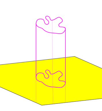
Figure 3. The cylinder over $[\gamma]$.

The embedded $\gamma(S^{1})$ comes with preferred parameterizations $[\gamma]$, and due to its linear structure ${\mathbb{R}}$ has several preferred parameterizations as well. For example given a number $T>0$ we can consider the following preferred parametrization of the infinite cylinder

(3.1) $${\mathbb{R}}\times S^{1}:(s,t)\rightarrow(Ts+c,\gamma(t+d)),$$

$$\text{where}\ c\in{\mathbb{R}}\ \text{and}\ \ d\in S^{1}.$$

There are modifications of the above which are being used later on. For example for the above we can derive some preferred parameterization covering the cylinder $k$-fold, obtained from the above by considering the preferred parameterizations

$$(s,t)\rightarrow(Ts+c,\gamma(kt+d)).$$

We note that $\bm{\gamma}:=([\gamma],T,k)$ captures the needed information.

Next we describe a basic idea in the case $([\gamma],T,1)$. We start by considering tuples $(\widetilde{u}^{+},\widetilde{u}^{-})$ where $\widetilde{u}^{\pm}:{\mathbb{R}}^{\pm}\times S^{1}\rightarrow{\mathbb{R}}\times{\mathbb{R}}^{N}$. Moreover these maps are continuous and have the following form

(3.2) $$\widetilde{u}^{+}(s,t)=(Ts+c^{+},\gamma(t+d^{+})+r^{+}(s,t))$$

$$\widetilde{u}^{-}(s^{\prime},t^{\prime})=(Ts^{\prime}+c^{-},\gamma(t+d^{-})+r^{-}(s,t)).$$

Here $r^{\pm}(s,t)\rightarrow 0$ as $s\rightarrow\pm\infty$, $c^{\pm}\in{\mathbb{R}}$ and $d^{\pm}\in S^{1}$. We see that the maps $\widetilde{u}^{\pm}$ approximate the cylinder associated to $[\gamma]$ as $s\rightarrow\pm\infty$, respecting in an approximate sense the preferred parameterizations. Assume for the moment $r^{\pm}=0$ and a large number $S>>0$ is given. We would like to construct from $\widetilde{u}^{\pm}$ which in some sense approximate the cylinder at their ends, a map on a long finite cylinder, which approximates the cylinder in its middle part. The whole process should produce no unnecessary wrinkles, i.e. in some sense should be as efficient as possible. To do so we glue $\widetilde{u}^{+}$ and the shifted $S\ast\widetilde{u}^{-}$, where we add $S$ to the first factor. In order to avoid wrinkles the gluing parameter for the domain has to be picked carefully. Our maps are $\widetilde{u}^{+}(s,t)=(Ts+c^{+},\gamma(t+d^{+}))$ and $S\ast\widetilde{u}^{-}(s^{\prime},t^{\prime})=(Ts^{\prime}+c^{-}+S,\gamma(t^{\prime}+d^{-}))$. There is only one way to glue these maps in a way which avoids wrinkles. Namely we define $R$ by

$$TR=S+c^{-}-c^{+}\ \ \text{and}\ \ d=d^{-}-d^{+}.$$

Then we define the glued map $\widetilde{w}$ on $Z_{(R,d)}$ by the usual formula

$$\widetilde{w}(\{(s,t),(s^{\prime},t^{\prime})\})$$

$$= \beta(s-R/2)\cdot\widetilde{u}^{+}(s,t)+\beta(-s^{\prime}-R/2)\cdot S\ast\widetilde{u}^{-}(s^{\prime},t^{\prime}).$$

We compute

$$\widetilde{w}(\{(s,t),(s^{\prime},t^{\prime})\})$$

$$= \beta(s-R/2)\cdot(Ts+c^{+},\gamma(t+d^{+}))$$

$$+\beta(-s^{\prime}-R/2)\cdot(T(s-R)+c^{-}+S,\gamma(t-d+d^{-}))$$

$$= (Ts+c^{+},\gamma(t+d^{+}))$$

If $r^{\pm}$ is nonzero we obtain from $\widetilde{u}^{\pm}$ the constants $c^{\pm}$ and $d=d^{-}-d^{+}$ from the asymptotic behavior of $\widetilde{u}^{\pm}$. Then for given $S>>0$ we can compute $R$ and use the gluing associated to $(R,d)$. Hence the modified $\widetilde{w}$ is given by

$$\widetilde{w}=(Ts+c^{-},\gamma(t+d^{+}))+\oplus(R,d,r^{+},r^{-}).$$

This defines

$$\bar{\oplus}(S,\widetilde{u}^{+},\widetilde{u}^{-})(\{(s,t),(s^{\prime},t^{\prime})\})$$

$$= \beta(s-R/2)\cdot\widetilde{u}^{+}(s,t)+\beta(-s^{\prime}-R/2)\cdot\widetilde{u}^{+}(s^{\prime},t^{\prime}).$$

Again, proper formulated, this will lead to an $\oplus$-construction. This time there is no global $f$ which partially inverts $\bm{\bar{\oplus}}$, but one can get away with two such maps. This time the constructions are more subtle as in the nodal case. The easier map is like in the nodal case, but the more interesting map is obtained as follows.

We are given $(S,\widetilde{w})$, where $\widetilde{w}:Z_{(R,d)}\rightarrow{\mathbb{R}}\times{\mathbb{R}}^{N}$ for $R>>0$ so that in addition the image of a middle-loop is close to the cylinder suitably parametrized, i.e. compatible with the distinguished coordinates. From the domain of $\widetilde{w}$ we extract the parameter $(R,d)$. By a subtle averaging construction we can find a candidate for $d^{+}$ which together with $d$ determines $d^{-}$. Using the averaging construction we obtain a candidate for $c^{+}$ and with the help of $S$ and $R$ we obtain $c^{-}$. Then we use a cut-off construction as in (2.1.1) to define an associated $\widetilde{w}^{\pm}$ obtained by transitioning from $\widetilde{w}$ to one of the distinguished parameterizations of the cylinder at infinity. Recall that in (2.1.1) we transitioned to a constant value. Our considerations in the following sections will also deal with the case that the cylinder associated to $[\gamma]$ is multiply-covered, i.e. a construction associated to $\bm{\gamma}=([\gamma],T,k)$.

Remark 3.1.

There are two versions of the above, which are equally valid. Above we glued $\widetilde{u}^{+}$ and $S\ast\widetilde{u}^{-}$. We can equally well also glue $(-S/2)\ast\widetilde{u}^{+}$ and $(S/2)\ast\widetilde{u}^{-}$, or $(-S)\ast\widetilde{u}^{+}$ and $\widetilde{u}^{-}$. Indeed, we shall utilize version 1 and version 3 in the case when we construct the M-polyfolds associated to symplectic cobordisms. Namely version 1 at the positive ends and version 3 at the negative ends. In the case of symplectizations one can take any of these versions. However, the fomulae for iterated constructions (more than two maps) get more cumbersome for version 2 and our choice is the version 1 gluing. One should point out that in this context one deals with maps modulo the ${\mathbb{R}}$-action $\ast$, so that the different versions only produce different representatives, which are mod ${\mathbb{R}}$ identical.

3.1.2. Constructions around Periodic Orbits

We begin with the definition of a periodic orbit.

Definition 3.2.

A periodic orbit in ${\mathbb{R}}^{N}$ is a tuple $\bm{\gamma}=([\gamma],T,k)$, where $T$ is a positive real number, $k\geq 1$ a positive integer, $\gamma:S^{1}\rightarrow{\mathbb{R}}^{N}$ a smooth embedding, and $[\gamma]$ denotes the set of reparameterizations $t\rightarrow\gamma(t+\theta)$ with $\theta\in S^{1}$. $T$ is called the period and $k$ the covering number. The number $T_{0}=T/k$ is called the minimal period. A weighted periodic orbit $\bm{\bar{\gamma}}$ (in ${\mathbb{R}}^{N}$) is a tuple $(\bm{\gamma},\delta)$, where $\delta={(\delta_{i})}_{i=0}^{\infty}$ is a strictly increasing sequence of weights $0<\delta_{0}<\delta_{1}<..<\delta_{i}<\delta_{i+1}$. There are obvious generalization to a notion of periodic orbit in a smooth manifold $Q$, where we require that $\gamma:S^{1}\rightarrow Q$ is an embedding.

There are several natural forgetful maps of interest to us, namely $\bm{\bar{\gamma}}\rightarrow\bm{\gamma}$, $\bm{\bar{\gamma}}\rightarrow\delta$ and $\bm{\bar{\gamma}}\rightarrow\delta_{0}$. In a moment we will define a so-called collection of standard maps, however before doing so it will be useful to recall the following preliminaries. Given a disk $D_{x}$ with $x\in D_{x}\setminus\partial D_{x}$, we let $\widehat{x}\subset T_{x}D_{x}$ denote an oriented line passing through $0\in T_{x}D_{x}$, and call $\widehat{x}$ a decoration. The set of all decorations in $T_{x}D_{x}$ is denoted $\mathbb{S}_{x}$. Given an ordered disk pair $((D_{x},D_{y}),(x,y))$, we say that $\{\widehat{x},\widehat{y}\}$ and $\{\widehat{x}^{\prime},\widehat{y}^{\prime}\}$ are equivalent provided $\widehat{x},\widehat{x}^{\prime}\in\mathbb{S}_{x}$ and $\widehat{y},\widehat{y}^{\prime}\in\mathbb{S}_{y}$ satisfy

$$\widehat{x}^{\prime}=e^{2\pi i\theta}\widehat{x}\qquad\text{and}\qquad\widehat{y}^{\prime}=e^{-2\pi i\theta}\widehat{y},$$

for some $\theta\in S^{1}$. It can be shown that our notion of equivalency does indeed define an equivalence relation, and we let $[\widehat{x},\widehat{y}]$ denote the equivalence class associated to $\{\widehat{x},\widehat{y}\}$. We call such an $[\widehat{x},\widehat{y}]$ a natural angle, and the set of natural angles is denoted by $\mathbb{S}_{x,y}$. Further details can be found in Appendix B.1. With these notions recalled, we are now prepared to define the collection of standard maps associated to a periodic orbit.

Definition 3.3.

Let ${\mathcal{D}}=((D_{x},D_{y}),(x,y))$ be an ordered disk pair. Given a periodic orbit $\bm{\gamma}$ in ${\mathbb{R}}^{N}$, the associated collection of standard maps in ${\mathbb{R}}\times{\mathbb{R}}^{N}$ is the set $\mathsf{S}_{\bm{\gamma}}$ consisting of tuples $(\widetilde{q}^{x},[\widehat{x},\widehat{y}],\widetilde{q}^{y})$, where $[\widehat{x},\widehat{y}]\in\mathbb{S}_{x,y}$ is a natural angle, and

$$\tilde{q}^{x}:D_{x}\setminus\{x\}\to\mathbb{R}\times\mathbb{R}^{N}$$

$$\tilde{q}^{y}:D_{y}\setminus\{y\}\to\mathbb{R}\times\mathbb{R}^{N},$$

satisfying the following conditions. There exists $\gamma\in[\gamma]$, $c^{x},c^{y}\in\mathbb{R}$, and representative $\{\widehat{x},\widehat{y}\}\in[\widehat{x},\widehat{y}]$ for which the following holds.

(3.4) $$\widetilde{q}^{x}\circ\sigma_{\widehat{x}}^{+}(s,t) = (Ts+c^{x},\gamma(kt))\in{\mathbb{R}}\times{\mathbb{R}}^{N}$$

$$\widetilde{q}^{y}\circ\sigma_{\widehat{y}}^{-}(s^{\prime},t^{\prime}) = (Ts^{\prime}+c^{y},\gamma(kt^{\prime}))\in{\mathbb{R}}\times{\mathbb{R}}^{N};$$

here $\sigma_{\widehat{x}}^{+}$ and $\sigma_{\widehat{y}}^{-}$ are as in equation (2.13) and equation (2.14)

Given a periodic orbit $\bm{\gamma}$ in ${\mathbb{R}}^{N}$ we have for every representative $\gamma$ in $[\gamma]$ a canonical map

$$\phi_{\gamma}:{\mathbb{R}}\times{\mathbb{S}}_{x}\times{\mathbb{R}}\times{\mathbb{S}}_{y}\rightarrow\mathsf{S}_{\bm{\gamma}}$$

defined by $\phi_{\gamma}(c^{x},\widehat{x},c^{y},\widehat{y})=(\widetilde{q}^{\gamma}_{c^{x},\widehat{x}},[\widehat{x},\widehat{y}],\widetilde{q}^{\gamma}_{c^{y},\widehat{y}})$, where

(3.5) $$\widetilde{q}^{\gamma}_{c^{x},\widehat{x}}\circ\sigma^{+}_{\widehat{x}}(s,t)=(Ts+c^{x},\gamma(kt))$$

$$\widetilde{q}^{\gamma}_{c^{y},\widehat{y}}\circ\sigma^{-}_{\widehat{y}}(s^{\prime},t^{\prime})=(Ts^{\prime}+c^{y},\gamma(kt^{\prime})).$$

The map $\phi_{\gamma}$ is $k:1$ and surjective. The cyclic group ${\mathbb{Z}}_{k}=\{0,...,k-1\}$ acts freely on $\widetilde{\Sigma}_{x,y}:={\mathbb{R}}\times{\mathbb{S}}_{x}\times{\mathbb{R}}\times{\mathbb{S}}_{y}$ via

$$j\ast(c^{x},\widehat{x},c^{y},\widehat{y})=(c^{x},e^{2\pi i(j/k)}\cdot\widehat{x},c^{y},e^{-2\pi i(j/k)}\cdot\widehat{y}).$$

Proposition 3.4.

Given $\bm{\gamma}=([\gamma],T,k)$ the set $\mathsf{S}_{\bm{\gamma}}$ admits a natural smooth manifold structure characterized by the property that for every $\gamma\in[\gamma]$, the map $\phi_{\gamma}:\widetilde{\Sigma}_{x,y}\rightarrow\mathsf{S}_{\gamma}$ is a local diffeomorphism. The preimage of a point under $\phi_{\gamma}$ is a ${\mathbb{Z}}_{k}$-orbit and the quotient $\Sigma_{x,y}=\widetilde{\Sigma}_{x,y}/{\mathbb{Z}}_{k}$ has a natural smooth manifold structure obtained by the standard procedure of dividing out the smooth ${\mathbb{Z}}_{k}$-action. The induced map $\Sigma_{x,y}\rightarrow\mathsf{S}_{\gamma}$ is a bijection and the desired smooth manifold structure on $\mathsf{S}_{\bm{\gamma}}$ is characterized by the requirement that this map is a diffeomorphism.

Proof.

Assume that $\phi_{\gamma}(c^{x},\widehat{x},c^{y},\widehat{y})=\phi_{\gamma}(d^{x},\widehat{x}^{\prime},d^{y},\widehat{y}^{\prime})$. We deduce that $[\widehat{x},\widehat{y}]=[\widehat{x}^{\prime},\widehat{y}^{\prime}]$ and therefore we find $\tau\in[0,1)$ such that

$$\widehat{x}^{\prime}=e^{2\pi i\tau}\cdot\widehat{x}\ \ \text{and}\ \ \widehat{y}^{\prime}=e^{-2\pi i\tau}\cdot\widehat{y}.$$

Moreover

$$(Ts+c^{x},\gamma(kt)) = \widetilde{q}^{x}_{c^{x},\widehat{x}}\circ\sigma^{+}_{\widehat{x}}(s,t)$$

$$= \widetilde{q}^{x}_{d^{x},\widehat{x}^{\prime}}\circ\sigma^{+}_{\widehat{x}}(s,t)$$

$$= \widetilde{q}^{x}_{d^{x},\widehat{x}^{\prime}}\circ\sigma^{+}_{\widehat{x}^{\prime}}(s,t-\tau)$$

$$= (Ts+d^{x},\gamma(k(t-\tau));)$$

where we have used the previously established fact that

$$h_{e^{2\pi i\tau}\widehat{x}}=e^{-2\pi i\tau}h_{\widehat{x}}$$

and hence

$$\sigma_{\widehat{x}^{\prime}}^{+}(s,t)=h_{\widehat{x}}^{-1}(e^{-2\pi(s+i(t-\tau))})=\sigma_{\widehat{x}}^{+}(s,t-\tau)).$$

This implies $k\tau=0$ mod $1$, and since $\tau\in[0,1)$ that $\tau=j/k$ for some $j\in\{0,...,k-1\}$. Further $c^{x}=d^{x}$. Similarly we show that

$$(Ts^{\prime}+c^{y},\gamma(kt^{\prime}))=(Ts^{\prime}+d^{y},\gamma(k(t^{\prime}-\tau))$$

implying that $\tau=j/k$ as before. This discussion shows that the preimage of a point is a ${\mathbb{Z}}_{k}$-orbit. The rest of the proof is obvious. ∎

Let $G$ be the automorphism group of the ordered ${\mathcal{D}}$. Then $G$ is diffeomorphic to $S^{1}\times S^{1}$ and acts on $\mathsf{S}_{\bm{\gamma}}$ via

$$g\ast(\widetilde{q}^{x},[\widehat{x},\widehat{y}],\widetilde{q}^{y}):=(\widetilde{q}^{x}\circ g^{-1},[Tg\cdot\widehat{x},Tg\cdot\widehat{y}],\widetilde{q}^{y}\circ g^{-1}).$$

This action is smooth since it corresponds under a $\Phi_{\gamma}$ to the smooth action $g\ast(c^{x},\widehat{x},c^{y},\widehat{y})=(c^{x},Tg\cdot\widehat{x},c^{y},Tg\cdot\widehat{y})$.

In a next step we introduce a set of maps which, as we shall show, has a natural ssc-manifold structure.

Definition 3.5.

Consider a map $\widetilde{w}:{\mathbb{R}}^{\pm}\times S^{1}\rightarrow{\mathbb{R}}\times{\mathbb{R}}^{N}$ and a periodic orbit $\bm{\gamma}$ in ${\mathbb{R}}^{N}$. We say that $\widetilde{w}$ is of class $H^{m,\tau}_{\bm{\gamma}}(\mathbb{R}^{\pm}\times S^{1},\mathbb{R}^{N})$ provided that there exists $\gamma\in[\gamma]$ and $c\in{\mathbb{R}}$ with the property that the map defined by

$$\widetilde{v}(s,t)=\widetilde{w}(s,t)-(Ts+c,\gamma(kt))$$

belongs to $H^{m,\tau}({\mathbb{R}}^{\pm}\times S^{1},{\mathbb{R}}^{N})$.

Definition 3.6.

Let ${\mathcal{D}}$ be an ordered disk pair and $\bm{\bar{\gamma}}=(\bm{\gamma},\delta)$ a weighted periodic orbit in ${\mathbb{R}}^{N}$. By $Z_{\mathcal{D}}^{3,\delta_{0}}({\mathbb{R}}\times{\mathbb{R}}^{N},\bm{{\gamma}})$ we denote the set which consists of all $(\widetilde{u}^{x},[\widehat{x},\widehat{y}],\widetilde{u}^{y})$ of class $(3,\delta_{0})$ converging to $\bm{\gamma}$ in a matching way. This means that $\widetilde{u}^{x}$ is of class $H^{3,\delta_{0}}_{\bm{\gamma}+}$, $\widetilde{u}^{y}$ of class $H^{3,\delta_{0}}_{\bm{\gamma}-}$ and $\widetilde{u}^{x}$ and $\widetilde{u}^{y}$ are $[\widehat{x},\widehat{y}]$-directionally matching. (see Appendix Definition and Definition ).

By $H^{3,\delta}({\mathcal{D}},{\mathbb{R}}\times{\mathbb{R}}^{N})$ we denote the sc-Hilbert space of maps of class $(3,\delta_{0})$ with vanishing asymptotic limit. We define the map

(3.6) $$\Psi:\mathsf{S}_{\bm{\gamma}}\times H^{3,\delta_{0}}({\mathcal{D}},{\mathbb{R}}\times{\mathbb{R}}^{N})\rightarrow Z^{3,\delta_{0}}_{\mathcal{D}}({\mathbb{R}}\times{\mathbb{R}}^{N},\bm{{\gamma}}):$$

$$(\widetilde{q},(\widetilde{h}^{x},\widetilde{h}^{y}))\rightarrow\widetilde{q}\dotplus(\widetilde{h}^{x},\widetilde{h}^{y}),$$

where the expression $\widetilde{q}\dotplus(\widetilde{h}^{x},\widetilde{h}^{y})$ for $\widetilde{q}=(\widetilde{q}^{x},[\widehat{x},\widehat{y}],\widetilde{q}^{y})$ is defined by

$$\widetilde{q}\dotplus(\widetilde{h}^{x},\widetilde{h}^{y})=(\widetilde{q}^{x}+\widetilde{h}^{x},[\widehat{x},\widehat{y}],\widetilde{q}^{y}+\widetilde{h}^{y}).$$

It is an easy exercise to verify the following lemma.

Lemma 3.7.

Let $\bm{\bar{\gamma}}$ be a weighted periodic orbit. Then the map $\Psi$ defined in (3.6) is a bijection.

As a consequence we obtain the following result.

Proposition 3.8.

Let $\bm{\bar{\gamma}}=(\bm{\gamma},\delta)$ be a weighted periodic orbit in ${\mathbb{R}}^{N}$ and ${\mathcal{D}}$ be an ordered disk pair. The set $Z^{3,\delta_{0}}_{\mathcal{D}}({\mathbb{R}}\times{\mathbb{R}}^{N},\bm{{\gamma}})$ has a natural ssc-manifold structure where the $m$-th level is given by regularity $(3+m,\delta_{m})$. This structure is characterized by the fact that the map $\Psi$ is a ssc-diffeomorphism. We shall write $Z_{\mathcal{D}}({\mathbb{R}}\times{\mathbb{R}}^{N},\bm{\bar{\gamma}})$ for the associated ssc-manifold.

The construction $Z_{\mathcal{D}}({\mathbb{R}}\times{\mathbb{R}}^{N},\bm{\bar{\gamma}})$ is part of a construction functor. Quite similar to a procedure described in Theorem 2.5 we have a canonical extension to target manifolds $Q$ equipped with a weighted periodic orbit. Namely, consider the category whose objects are pairs $({\mathbb{R}}^{N},\bm{\bar{\gamma}})$, where $\bm{\bar{\gamma}}$ is weighted periodic orbit in ${\mathbb{R}}^{N}$. A morphism

$$h:({\mathbb{R}}^{N},\bm{\bar{\gamma}})\rightarrow({\mathbb{R}}^{N^{\prime}},\bm{\bar{\gamma}^{\prime}})$$

consists of a smooth map $h:{\mathbb{R}}^{N}\rightarrow{\mathbb{R}}^{N^{\prime}}$, where with $\bm{\bar{\gamma}}=(([\gamma],T,k),\delta)$ we have that $\bm{\bar{\gamma}^{\prime}}=(([h\circ\gamma],T,k),\delta)$. Then with $\widetilde{h}=Id_{\mathbb{R}}\times h$ we obtain an induced map

$$\widetilde{h}_{\ast}:Z_{\mathcal{D}}({\mathbb{R}}\times{\mathbb{R}}^{N},\bm{\bar{\gamma}})\rightarrow Z_{\mathcal{D}}({\mathbb{R}}\times{\mathbb{R}}^{N^{\prime}},\bm{\bar{\gamma}^{\prime}}):\widetilde{u}\rightarrow\widetilde{h}\circ\widetilde{u}.$$

By considering the map on each level of regularity $(3+m,\delta_{m})$ we obtain a map between Hilbert manifolds and classical smoothness belongs to the realm of [13]. As a consequence we obtain the following result and the details of the proof are left the reader.

Proposition 3.9.

A morphism $h:({\mathbb{R}}^{N},\bm{\bar{\gamma}})\rightarrow({\mathbb{R}}^{N^{\prime}},\bm{\bar{\gamma}^{\prime}})$ induces an ssc-smooth map $\widetilde{h}_{\ast}:Z_{\mathcal{D}}({\mathbb{R}}\times{\mathbb{R}}^{N},\bm{\bar{\gamma}})\rightarrow Z_{\mathcal{D}}({\mathbb{R}}\times{\mathbb{R}}^{N^{\prime}},\bm{\bar{\gamma}^{\prime}})$.

The automorphism group $G_{\mathcal{D}}$ of the ordered disk pair ${\mathcal{D}}$ acts on the disks by individual rotations and hereby defines an action on $Z_{\mathcal{D}}({\mathbb{R}}\times{\mathbb{R}}^{N},\bm{\bar{\gamma}})$ via

$$g\ast(\widetilde{u}^{x},[\widehat{x},\widehat{y}],\widetilde{u}^{y})=(\widetilde{u}^{x}\circ g^{-1},[Tg\cdot\widehat{x},Tg\cdot\widehat{y}],\widetilde{u}^{y}\circ g^{-1}).$$

Via the map $\Psi$ this action corresponds to the sc-smooth action on $\mathsf{S}_{\bm{\gamma}}\times H^{3,\delta}({\mathcal{D}},{\mathbb{R}}\times{\mathbb{R}}^{N})$ defined by

$$g\ast(\widetilde{q},(\widetilde{h}^{x},\widetilde{h}^{y}))=(g\ast\widetilde{q},(\widetilde{h}^{x}\circ g^{-1},\widetilde{h}^{y}\circ g^{-1})).$$

Here we use the sc-smoothness of the $G$-action on $H^{3,\delta}({\mathcal{D}},{\mathbb{R}}\times{\mathbb{R}}^{N})$, see Proposition 2.10 and note that our space is an invariant finite co-dimension subspace. Hence we have established the following result.

Proposition 3.10.

Let $\bm{\bar{\gamma}}$ be a weighted periodic orbit, ${\mathcal{D}}$ be an ordered disk pair and assume that $Z_{\mathcal{D}}({\mathbb{R}}\times{\mathbb{R}}^{N},\bm{\bar{\gamma}})$ is the associated ssc-manifold. Then the action of the automorphism group $G$ of ${\mathcal{D}}$ is sc-smooth. The action is not(!) ssc-smooth.

Remark 3.11.

If $\bm{\bar{\gamma}}$ is a weighted periodic orbit in a manifold $Q$ without boundary, which can be properly embedded into some ${\mathbb{R}}^{N}$ we have a well-defined $Z_{\mathcal{D}}({\mathbb{R}}\times Q,\bm{\bar{\gamma}})$. Since the maps involved are ssc-smooth the procedure from Theorem 2.5 produces ssc-manifolds. We leave the details for this classical case to the reader.

Exercise 7.

Show that the construction $Z_{\mathcal{D}}$ which associates to $({\mathbb{R}}^{N},\bm{\bar{\gamma}})$ the ssc-manifold $Z_{\mathcal{D}}({\mathbb{R}}\times{\mathbb{R}}^{N},\bm{\bar{\gamma}})$ and to a morphism $h$ the ssc-smooth map $\widetilde{h}_{\ast}$ is a construction functor. Conclude using the ideas from Section that the construction has a natural extension to cover periodic orbits in manifolds, i.e. $(Q,\bm{\bar{\gamma}})$.

3.1.3. The M-Polyfold $Y_{{\mathcal{D}},\varphi}({\mathbb{R}}\times{\mathbb{R}}^{N},\bm{\bar{\gamma}})$

Consider the ssc-manifold with boundary

$$\mathfrak{Z}:=[0,1)\times Z_{\mathcal{D}}({\mathbb{R}}\times{\mathbb{R}}^{N},\bm{\bar{\gamma}})$$

and recall that given $(\widetilde{u}^{x},[\widehat{x},\widehat{y}],\widetilde{y}^{y})$ in $Z_{\mathcal{D}}({\mathbb{R}}\times{\mathbb{R}}^{N},\bm{\bar{\gamma}})$ we can write it uniquely as $(\widetilde{q}^{x}+\widetilde{h}^{x},[\widehat{x},\widehat{y}],\widetilde{q}^{y}+\widetilde{h}^{y})$, where $(\widetilde{q}^{x},[\widehat{x},\widehat{y}],\widetilde{q}^{y})$ is a standard map. We can extract the asymptotic constants $c^{x},c^{y}$ ssc-smoothly, i.e. the maps

$$\bar{c}^{x},\bar{c}^{y}:Z_{\mathcal{D}}({\mathbb{R}}\times{\mathbb{R}}^{N},\bm{\bar{\gamma}})\rightarrow{\mathbb{R}}$$

are ssc-smooth. We define an open neighborhood ${\mathcal{V}}$ of $\partial\mathfrak{Z}=\{0\}\times Z_{\mathcal{D}}({\mathbb{R}}\times{\mathbb{R}}^{N},\bm{\bar{\gamma}})$ in $\mathfrak{Z}$ as follows.

Definition 3.12.

The open subset ${\mathcal{V}}$ of $\mathfrak{Z}$ consists of all tuples

$$(r,(\widetilde{u}^{x},[\widehat{x},\widehat{y}],\widetilde{u}^{y}))=:(r,\widetilde{u})$$

such that either $r=0$, or in the case $r\in(0,1)$ the following holds.

• $\varphi(r)+c^{y}(\widetilde{u})-c^{x}(\widetilde{u})>0$.

• $\varphi^{-1}\left(\frac{1}{T}\cdot(\varphi(r)+c^{y}(\widetilde{u})-c^{x}(\widetilde{u}))\right)\in(0,1/4)$.

We note that ${\mathcal{V}}$ is a ssc-manifold with boundary. An important map is $\bar{r}:{\mathcal{V}}\rightarrow[0,1):(r,\widetilde{u})\rightarrow r.$ This is the restriction of the projection onto the first factor $[0,1)\times Z_{\mathcal{D}}({\mathbb{R}}\times{\mathbb{R}}^{N},\bm{\bar{\gamma}})\rightarrow[0,1)$ onto an open subset. Since the latter map is submersive the same holds for $\bar{r}$. It is clear that $\bar{r}$ is surjective. Hence we obtain.

Lemma 3.13.

The map

$$\bar{r}:{\mathcal{V}}\rightarrow[0,1):(r,\widetilde{u})\rightarrow r.$$

is a surjective and submersive ssc-smooth map.

Recall the M-polyfold $X^{3,\delta}_{{\mathcal{D}},\varphi}({\mathbb{R}}\times{\mathbb{R}}^{N})$ with submersive map

$$p_{\mathbb{B}}:X^{3,\delta}_{{\mathcal{D}},\varphi}({\mathbb{R}}\times{\mathbb{R}}^{N})\rightarrow{\mathbb{B}}$$

introduced in the previous Section 2. We denote by $\dot{X}^{3,\delta}_{{\mathcal{D}},\varphi}({\mathbb{R}}\times{\mathbb{R}}^{N})$ the preimage of ${\mathbb{B}}\setminus\{0\}$ under $p_{\mathbb{B}}$. We have already discussed earlier that the set $\dot{X}^{3,\delta}_{{\mathcal{D}},\varphi}({\mathbb{R}}\times{\mathbb{R}}^{N})$ does neither depend on $\varphi$ nor $\delta$ and the same is true for the induced M-polyfold structure as an open subset, see Remarks 2.9 and 2.16. For that reason we denote this M-polyfold, which also has a natural sc-manifold structure inducing the M-polyfold structure in question, by $\dot{X}_{\mathcal{D}}({\mathbb{R}}\times{\mathbb{R}}^{N})$, see Exercise 2.

Definition 3.14.

The M-polyfold $\mathfrak{X}$ is by definition the open subset of $(0,1)\times{X}^{3,\delta}_{{\mathcal{D}},\varphi}({\mathbb{R}}\times{\mathbb{R}}^{N})$ defined as

$$\mathfrak{X}=(0,1)\times\dot{X}_{\mathcal{D}}({\mathbb{R}}\times{\mathbb{R}}^{N})$$

and equipped with the induced M-polyfold structure. As we just noted before the latter comes, in fact, from a uniquely natural defined sc-manifold structure. We note that the degeneracy index associated to $\mathfrak{X}$ vanishes identically.

Next we define the set $Y^{3,\delta_{0}}_{{\mathcal{D}},\varphi}({\mathbb{R}}\times{\mathbb{R}}^{N},\bm{\gamma})$ we are interested in, and which we shall equip with a M-polyfold structure by the $\oplus$-method.

Definition 3.15.

Given an ordered disk pair ${\mathcal{D}}$ and a weighted periodic orbit $\bm{\bar{\gamma}}$ in ${\mathbb{R}}^{N}$ the set $Y^{3,\delta_{0}}_{{\mathcal{D}},\varphi}:=Y^{3,\delta_{0}}_{{\mathcal{D}},\varphi}({\mathbb{R}}\times{\mathbb{R}}^{N},\bm{\gamma})$ is defined as the disjoint union

$$Y^{3,\delta_{0}}_{{\mathcal{D}},\varphi}=\left(\{0\}\times Z^{3,\delta_{0}}_{\mathcal{D}}({\mathbb{R}}\times{\mathbb{R}}^{N},\bm{\gamma})\right)\coprod\mathfrak{X}=\partial\mathfrak{Z}\coprod\mathfrak{X}.$$

Remark 3.16.

We observe that the space is a union of a ssc-manifold $\partial\mathfrak{Z}$, provided we use the full $\delta$, and a sc-manifold $\mathfrak{X}$. Our aim is to define a natural (up to a choice of the gluing profile $\varphi$) M-polyfold structure on $Y^{3,\delta_{0}}_{{\mathcal{D}},\varphi}$ in such a way that $\mathfrak{X}$ is an open and dense sub-M-polyfold with the induced structure being the original one. Moreover, also $\partial\mathfrak{Z}$ will be a sub-M-polyfold and the induced structure will be the M-polyfold structure diffeomorphic to the sc-structure derived from the original ssc-manifold structure.

In order to define a M-polyfold structure on $Y^{3,\delta_{0}}_{{\mathcal{D}},\varphi}$ we shall use the $\oplus$-method. This case will turn out to be somewhat more involved than the nodal case since we need to construct two maps defined on open subsets (for the quotient topology) of $Y^{3,\delta_{0}}_{{\mathcal{D}},\varphi}$ rather than the single $f$ in the nodal case.

The set ${\mathcal{V}}$ introduced in Definition 3.12 has naturally the structure of a ssc-manifold and we shall define a map

(3.7) $$\bm{\bar{\oplus}}:{\mathcal{V}}\rightarrow Y^{3,\delta_{0}}_{{\mathcal{D}},\varphi},$$

where the right-hand side for the moment is viewed as just a set.

Definition 3.17.

The map $\mathsf{a}:{\mathcal{V}}\rightarrow{\mathbb{B}}$ is defined by associating to the tuple $(0,(\widetilde{u}^{x},[\widehat{x},\widetilde{y}],\widetilde{u}^{y}))$ the element $0$ and in the case $r\neq 0$ the element $a=|a|\cdot[\widehat{x},\widehat{y}]$, where

$$T\cdot\varphi(|a|)=\varphi(r)+c^{y}-c^{x}.$$

Here $c^{x}=c^{x}(\widetilde{u}^{x})$ and $c^{y}=c^{y}(\widetilde{u}^{y})$.

As a consequence of [38], Lemma 4.4, the following holds.

Lemma 3.18.

The map $\mathsf{a}:{\mathcal{V}}\rightarrow{\mathbb{B}}$ is ssc-smooth.

Now we begin with the crucial construction.

Definition 3.19.

The map $\bm{\bar{\oplus}}:{\mathcal{V}}\rightarrow Y^{3,\delta_{0}}_{{\mathcal{D}},\varphi}({\mathbb{R}}\times{\mathbb{R}}^{N},\bm{\gamma})$ is defined as follows. We put, if $r=0$,

$$\bm{\bar{\oplus}}(0,(\widetilde{u}^{x},[\widehat{x},\widehat{y}],\widetilde{u}^{y}))=(0,\bar{\oplus}(0,(\widetilde{u}^{x},[\widehat{x},\widehat{y}],\widetilde{u}^{y})))=(0,(\widetilde{u}^{x},[\widehat{x},\widehat{y}],\widetilde{u}^{y})).$$

If $r\neq 0$ we define

(3.8) $$\bm{\bar{\oplus}}(r,(\widetilde{u}^{x},[\widehat{x},\widehat{y}],\widetilde{u}^{y}))=(r,\bar{\oplus}(r,(\widetilde{u}^{x},[\widehat{x},\widehat{y}],\widetilde{u}^{y})))=(r,\widetilde{w})$$

where, with $a=\mathsf{a}(r,(\widetilde{u}^{x},[\widehat{x},\widetilde{y}],\widetilde{u}^{y}))$, the map $\widetilde{w}:Z_{a}\rightarrow{\mathbb{R}}\times{\mathbb{R}}^{N}$ is given by

$$\widetilde{w}(z,z^{\prime})=\beta^{x}_{a}(z)\cdot\widetilde{u}^{x}(z)+\beta^{y}_{a}(z^{\prime})\cdot(\varphi(r)\ast\widetilde{u}^{y}(z^{\prime})).$$

Above, $``\ast"$ denotes the additive ${\mathbb{R}}$-action on the first factor.

Here is the main result in this subsection, which will be proved later.

Theorem 3.20.

Let ${\mathcal{D}}$ be an ordered disk pair and $\bm{\bar{\gamma}}$ a weighted periodic orbit in ${\mathbb{R}}^{N}$. The map $\bm{\bar{\oplus}}:{\mathcal{V}}\rightarrow Y^{3,\delta_{0}}_{{\mathcal{D}},\varphi}({\mathbb{R}}\times{\mathbb{R}}^{N},\bm{\gamma})$ is a M-polyfold construction by the $\oplus$-method fitting into the commutative diagram

$$\begin{CD}{\mathcal{V}}@>{\bm{\bar{\oplus}}}>{}>Y^{3,\delta_{0}}_{{\mathcal{D}},\varphi}({\mathbb{R}}\times{\mathbb{R}}^{N},\bm{\gamma})\\ @V{pr_{1}}V{}V@V{\bar{r}}V{}V\\ [0,1)\ \ \ \ @=[0,1),\end{CD}$$

where the vertical arrows are the obvious extractions of the $r$-parameter. Moreover the following holds.

• For the defined M-polyfold structure an element $(r,\widetilde{u})$ has degeneracy index $1$ if $r=0$ and $0$ otherwise.

• The M-polyfold structure is tame.

Proof.

The proof of Theorem 3.20 is given in Subsection 3.6.1, but requires a considerable amount of preparation provided in the following sections. ∎

Recall that the set $Y^{3,\delta_{0}}_{{\mathcal{D}},\varphi}({\mathbb{R}}\times{\mathbb{R}}^{N},\bm{\gamma})$ is the disjoint union of $\partial\mathfrak{Z}$ and $\mathfrak{X}$, where $\partial\mathfrak{Z}$ has already a ssc-manifold structure and $\mathfrak{X}$ a sc-manifold structure. The $\bm{\bar{\oplus}}$-structure will be related to the already existing structures. The following theorem summarizes the additional properties, where ${\mathcal{T}}$ is the quotient topology underlying the M-polyfold structure arising from Theorem 3.20.

Definition 3.21.

The set $Y^{3,\delta_{0}}_{{\mathcal{D}},\varphi}({\mathbb{R}}\times{\mathbb{R}}^{N},\bm{\gamma})$ equipped with the M-polyfold structure resulting from Theorem 3.22 via

$$\bm{\bar{\oplus}}:{\mathcal{V}}\rightarrow Y^{3,\delta_{0}}_{{\mathcal{D}},\varphi}({\mathbb{R}}\times{\mathbb{R}}^{N},\bm{\gamma})$$

is denoted by $Y^{3,\delta}_{{\mathcal{D}},\varphi}({\mathbb{R}}\times{\mathbb{R}}^{N},\bm{\bar{\gamma}})$, or, more explicitly, $Y_{{\mathcal{D}},\varphi}^{3,\delta}({\mathbb{R}}\times{\mathbb{R}}^{N},\bm{\gamma})$.

Recall that the subsets $\partial\mathfrak{Z}$ and $\mathfrak{X}$ of $Y^{3,\delta}_{{\mathcal{D}},\varphi}({\mathbb{R}}\times{\mathbb{R}}^{N},\bm{\bar{\gamma}})$ already possessed previously defined structures, see Remark 3.16. The following Theorem 3.22 and Proposition 3.23 show that the new construction recovers the original structures in a suitable sense. In addition they show that the M-polyfold structure does not depend on the choice of the cut-off model $\beta$.

Theorem 3.22.

The $\bm{\bar{\oplus}}$-polyfold structure on $Y^{3,\delta_{0}}_{{\mathcal{D}},\varphi}({\mathbb{R}}\times{\mathbb{R}}^{N},\bm{\gamma})$ has the following properties.

• The topologies induced by ${\mathcal{T}}$ on $\mathfrak{X}$ and $\partial\mathfrak{Z}$ are the original topologies for the already existing sc-manifold structure on $\mathfrak{X}$ and ssc-manifold structure on $\partial\mathfrak{Z}$.

• The M-polyfold structure on $Y^{3,\delta_{0}}_{{\mathcal{D}},\varphi}({\mathbb{R}}\times{\mathbb{R}}^{N},\bm{\gamma})$ does not(!) depend on the smooth $\beta:{\mathbb{R}}\rightarrow[0,1]$ which was taken in the definition of $\bm{\bar{\oplus}}$ as long as it satisfies the usual properties $\beta(s)+\beta(-s)=1$, $\beta(s)=1$ for $s\leq-1$, and $\beta^{\prime}(s)<0$ for $s\in(-1,1)$.

Proof.

The proof of Theorem 3.22 is given in Subsection 3.6.1 together with the proof of Theorem 3.20. Both need some common preparation provided in the coming sections. ∎

The following result will be a corollary of Theorem 3.36 which will be stated and proved later.

Proposition 3.23.

The following holds.

• The subset $\mathfrak{X}$ of $Y_{{\mathcal{D}},\varphi}({\mathbb{R}}\times{\mathbb{R}}^{N},\bm{\bar{\gamma}})$ is open and dense for the topology ${\mathcal{T}}$ and the induced M-polyfold structure is the original existing one.

• The subset $\partial\mathfrak{Z}$ is closed for the topology ${\mathcal{T}}$ and carries the structure of a sub-M-polyfold which is the M-polyfold structure induced by the original ssc-manifold structure.

Proof.

Follows from Theorem 3.36. See also the end of Subsection 3.6.1. ∎

For later constructions we introduce several maps. The first one already occurred in the statement of Theorem 3.20.

Definition 3.24.

We have the following canonical maps:

• $\bar{r}:Y_{{\mathcal{D}},\varphi}({\mathbb{R}}\times{\mathbb{R}}^{N},\bm{\bar{\gamma}})\rightarrow[0,1)$ extracts the parameter $r$.

• $\bar{a}_{d}:Y_{{\mathcal{D}},\varphi}({\mathbb{R}}\times{\mathbb{R}}^{N},\bm{\bar{\gamma}})\rightarrow[0,1/4)\times{\mathbb{S}}$ extracts the decorated domain gluing parameter $(|a|,[\widehat{x},\widehat{y}])$.

• $\bar{a}:Y_{{\mathcal{D}},\varphi}({\mathbb{R}}\times{\mathbb{R}}^{N},\bm{\bar{\gamma}})\rightarrow{\mathbb{B}}$ extracts the domain gluing parameter $a=|a|\cdot[\widehat{x},\widehat{y}]=:m\circ\bar{a}_{d}(|a|,[\widehat{x},\widehat{y}])$, where $m(b,[\widehat{x},\widehat{y}])=b\cdot[\widehat{x},\widehat{y}]$.

The following proposition summarizes the properties of the three maps and follows from Proposition 3.65 stated later on.

Proposition 3.25.

The following holds.

• For the previously defined M-polyfold structure on $Y_{{\mathcal{D}},\varphi}({\mathbb{R}}\times{\mathbb{R}}^{N},\bm{\bar{\gamma}})$ the natural maps $\bar{r}$, $\bar{a}_{d}$, and $\bar{a}$ are sc-smooth.

• The map $\bar{r}$ is submersive.

Proof.

Follows from Proposition 3.65. ∎

3.1.4. Extensions to Manifolds

In the construction of $Y_{{\mathcal{D}},\varphi}({\mathbb{R}}\times{\mathbb{R}}^{N},\bm{\bar{\gamma}})$ we would like to replace $({\mathbb{R}}^{N},\bm{\bar{\gamma}})$ by a periodic orbit in some manifold $Q$, in order to define a M-polyfold denoted by $Y_{{\mathcal{D}},\varphi}({\mathbb{R}}\times Q,\bm{\bar{\gamma}})$ In order to do we will proceed as in the nodal case. Namely we show that the construction $Y_{{\mathcal{D}},\varphi}$ defines a functor on the category having pairs $({\mathbb{R}}^{N},\bm{\bar{\gamma}})$ as objects and suitable morphisms based on smooth maps between them. Then the idea from Subsection can be applied.

Consider first the category ${\mathcal{P}}_{w}^{0}$, whose objects are pairs $({\mathbb{R}}^{N},\bm{\bar{\gamma}})$, where $\bm{\bar{\gamma}}$ is a weighted periodic orbit in ${\mathbb{R}}^{N}$. A morphism $({\mathbb{R}}^{N},\bm{\bar{\gamma}})\rightarrow({\mathbb{R}}^{N^{\prime}},\bm{\bar{\gamma}}^{\prime})$ only exists provided $(\delta,T,k)=(\delta^{\prime},T^{\prime},k^{\prime})$ and is given by a smooth map $h:{\mathbb{R}}^{N}\rightarrow{\mathbb{R}}^{N^{\prime}}$ having the property that $h\circ\gamma\in[\gamma^{\prime}]$ for $\gamma\in[\gamma]$. Associated to $h$ we have the map $\widetilde{h}=Id_{\mathbb{R}}\times h:{\mathbb{R}}\times{\mathbb{R}}^{N}\rightarrow{\mathbb{R}}\times{\mathbb{R}}^{N^{\prime}}$. We define

$$\widetilde{h}_{\ast}:Y_{{\mathcal{D}},\varphi}({\mathbb{R}}\times{\mathbb{R}}^{N},\bm{\bar{\gamma}})\rightarrow Y_{{\mathcal{D}},\varphi}({\mathbb{R}}\times{\mathbb{R}}^{N^{\prime}},\bm{\bar{\gamma}}^{\prime})$$

by $(r,\widetilde{w})\rightarrow(r,\widetilde{h}\circ\widetilde{w})$ if $r\in(0,1)$ and $(0,(\widetilde{u}^{x},[\widehat{x},\widehat{y}],\widetilde{u}^{y}))\rightarrow(0,(\widetilde{h}\circ\widetilde{u}^{x},[\widehat{x},\widehat{y}],\widetilde{h}\circ\widetilde{u}^{y}))$. The following holds.

Proposition 3.26.

Let $h:({\mathbb{R}}^{N},\bm{\bar{\gamma}})\rightarrow({\mathbb{R}}^{N^{\prime}},\bm{\bar{\gamma}}^{\prime})$ be a morphism. Then the map

$$\widetilde{h}_{\ast}:Y_{{\mathcal{D}},\varphi}({\mathbb{R}}\times{\mathbb{R}}^{N},\bm{\bar{\gamma}})\rightarrow Y_{{\mathcal{D}},\varphi}({\mathbb{R}}\times{\mathbb{R}}^{N^{\prime}},\bm{\bar{\gamma}}^{\prime})$$

is sc-smooth and $\widetilde{(h^{\prime}\circ h)}_{\ast}=\widetilde{h}^{\prime}_{\ast}\circ\widetilde{h}_{\ast}$ if $h^{\prime}$ is another morphism composeable with $h$. Also $\widetilde{Id}_{\ast}=Id$.

Proof.

This follows from Proposition 3.66. ∎

Now it is clear that we can use the procedure of the previous section to extend our construction to pairs $(Q,\bm{\bar{\gamma}})$.

Definition 3.27.

Let $Q$ be a smooth connected manifold without boundary which allows a proper embedding into some ${\mathbb{R}}^{N}$. A periodic orbit in $Q$ is a tuple $\bm{\gamma}=([\gamma],T,k)$, where $\gamma:S^{1}\rightarrow Q$ is a smooth embedding and $[\gamma]$ consists of all parameterizations of the form $t\rightarrow\gamma(t+\theta)$. As in the ${\mathbb{R}}^{N}$-case we can define weighted periodic orbits $\bm{\bar{\gamma}}=(\bm{\gamma},\delta)$.

We consider the category $\mathcal{P}_{w}$ whose objects are pairs $(Q,\bm{\bar{\gamma}})$ as just described. Morphisms $(Q,\bm{\bar{\gamma}})\rightarrow(Q^{\prime},\bm{\bar{\gamma}}^{\prime})$ only exist if $\delta=\delta^{\prime}$, $(T,k)=(T^{\prime},k^{\prime})$, and this case they are given by a smooth map $h:Q\rightarrow Q^{\prime}$ such that for $\gamma\in[\gamma]$ the map $h\circ\gamma\in[\gamma^{\prime}]$.

Theorem 3.28.

The polyfold construction $Y_{{\mathcal{D}},\varphi}({\mathbb{R}}\times{\mathbb{R}}^{N},\bm{\bar{\gamma}})$ for pairs $({\mathbb{R}}^{N},\bm{\bar{\gamma}})$ and the morphisms between them extends to a functorial construction defined on ${\mathcal{P}}_{w}$.

Proof.

The idea follows along the line of the construction functor ”technology” used already in the nodal case, see also Section We sketch the proof. $Y_{{\mathcal{D}},\varphi}({\mathbb{R}}\times Q,\bm{\bar{\gamma}})$ is defined by taking a proper embedding $\phi:Q\rightarrow{\mathbb{R}}^{N}$ for a suitable $N$. With $\bm{\bar{\gamma}}=(([\gamma],T,k),\delta)$ we define $\bm{\bar{\gamma}^{\prime}}=(([\gamma^{\prime}],T,k),\delta)$, where $\gamma^{\prime}=\phi\circ\gamma$. We consider the subset $\Sigma_{\phi}$ of $Y_{{\mathcal{D}},\varphi}({\mathbb{R}}\times{\mathbb{R}}^{N},\bm{\bar{\gamma}^{\prime}})$ consisting of tuples $(r,\widetilde{u})$ with $\widetilde{u}$ having image in ${\mathbb{R}}\times\phi(Q)$. The set $\Sigma_{\phi}$ is a sub-M-polyfold using the ideas described in Section 2. Then $Y_{{\mathcal{D}},\varphi}({\mathbb{R}}\times Q,\bm{\bar{\gamma}})$ is the set of tuples $(r,\widetilde{v})$, where $\widetilde{v}$ is a map into ${\mathbb{R}}\times Q$, so that $(r,(Id\times\phi)\circ\widetilde{v})\in\Sigma_{\phi}$. The M-polyfold structure is the one making it a sc-diffeomorphism. We leave the details to the reader since it follows closely the already explained construction functor idea, see the next exercise. ∎

Exercise 8.

Carry out the proof of Theorem 3.28 in more detail assuming Proposition 3.26.

In the following subsections we shall provide the basic constructions which we just presented.

3.2. The Coretraction $H$

We have to study

(3.9) $$\bm{\bar{\oplus}}:{\mathcal{V}}\rightarrow Y^{3,\delta_{0}}_{{\mathcal{D}},\varphi}({\mathbb{R}}\times{\mathbb{R}}^{N},\bm{\gamma})$$

and show that it defines a M-polyfold structure on $Y^{3,\delta_{0}}_{{\mathcal{D}},\varphi}({\mathbb{R}}\times{\mathbb{R}}^{N},\bm{\gamma})$ by the $\oplus$-method. As we have previously mentioned we need to construct two maps in order to show that $\bm{\bar{\oplus}}$ is an $\oplus$-construction. These maps denoted by $H$ and $K$ provided the local $H_{y}$ by restriction as they occur in Definition Since we also want to prove some additional properties we have to take special care. The set $Y^{3,\delta_{0}}_{{\mathcal{D}},\varphi}$ is the disjoint union of $\partial\mathfrak{Z}$ and $\mathfrak{X}$, which already have certain sc-smooth structures and our aim is to find a M-polyfold structure on the whole set which induces on these subsets the already existing structures. We shall denote by ${\mathcal{T}}$ the quotient topology on $Y^{3,\delta_{0}}_{{\mathcal{D}},\varphi}({\mathbb{R}}\times{\mathbb{R}}^{N},\bm{\gamma})$ associated to (3.9).

Recall from Section 2, Remarks 2.9 and 2.16 the following fact which we shall use repeatedly.

Fact 3.29.

The space

$$\dot{X}^{3}_{{\mathcal{D}}}({\mathbb{R}}\times{\mathbb{R}}^{N}):=\{\widetilde{w}\in{X}^{3}_{{\mathcal{D}}}\ |\ a(\widetilde{w})\in{\mathbb{B}}\setminus\{0\}\}$$

has a M-polyfold structure characterized by

$$\oplus:({\mathbb{B}}\setminus\{0\})\times H^{3,\delta}({\mathcal{D}},{\mathbb{R}}\times{\mathbb{R}}^{N})\rightarrow\dot{X}^{3}_{{\mathcal{D}}}({\mathbb{R}}\times{\mathbb{R}}^{N})$$

where

$$\oplus(a,\widetilde{h}^{x},\widetilde{h}^{y})(z,z^{\prime})=\beta^{x}_{a}(z)\cdot\widetilde{h}^{x}(z)+\beta^{y}_{a}(z^{\prime})\cdot\widetilde{h}^{y}(z^{\prime}).$$

The $\oplus$-method gives a well-defined M-polyfold structure on $\dot{X}^{3}_{{\mathcal{D}}}({\mathbb{R}}\times{\mathbb{R}}^{N})$. This structure has the property that the map $\oplus$ is sc-smooth, surjective, and open, and admits an sc-smooth $f$ such that $\oplus\circ f=Id$. This was previously discussed. As already previously mentioned we can also define a natural sc-manifold structure on $\dot{X}^{3}_{{\mathcal{D}}}({\mathbb{R}}\times{\mathbb{R}}^{N})$, see Exercise 2. More details are also given in Subsection The identity map is an sc-diffeomorphism between the two structures.

By construction $\mathfrak{X}=(0,1)\times\dot{X}^{3}_{{\mathcal{D}}}({\mathbb{R}}\times{\mathbb{R}}^{N})$ and in view of the previous fact it has a M-polyfold structure coming from a sc-manifold structure. We always view $\mathfrak{X}$ as being equipped with this M-polyfold structure. Clearly the structure on $\mathfrak{X}$ can also be obtained by the $\oplus$-method. The surjective map in this case is $Id_{(0,1)}\times\oplus:(0,1)\times(({\mathbb{B}}\setminus\{0\})\times H^{3,\delta}({\mathcal{D}},{\mathbb{R}}\times{\mathbb{R}}^{N}))\rightarrow\mathfrak{X}$.

Aim 3.30 (1).

We shall construct with ${\mathcal{V}}$ given in Definition 3.12 a map $H:\mathfrak{X}\rightarrow{\mathcal{V}}$ preserving the fiber over $(0,1)$, i.e. fitting into the commutative diagram

$$\begin{CD}\mathfrak{X}@>{H}>{}>{\mathcal{V}}\\ @V{pr_{1}}V{}V@V{\bar{r}}V{}V\\ (0,1)@>{}>{}>[0,1),\end{CD}$$

such that $H$ is sc-smooth (for the already existing M-polyfold structure on $\mathfrak{X}$) and $\bm{\bar{\oplus}}\circ H=Id_{\mathfrak{X}}$, where $\bm{\bar{\oplus}}$ is introduced in Definition 3.19.

We fix a representative $\gamma_{0}$ in $[\gamma]$, a decoration $\widehat{x}_{0}$, and consider with $c^{x}=0$ the associated $\widetilde{q}_{0,\widehat{x}_{0}}^{\gamma_{0}}$ defined in (3.5). Given $(r,\widetilde{w})\in\mathfrak{X}$ let $a=a(\widetilde{w})$, $R=\varphi(|a|)$, and write $a=|a|\cdot[\widehat{x}_{0},\widehat{y}]$. We define $H(r,\widetilde{w})=(r,(\widetilde{u}^{x},[\widehat{x}_{0},\widehat{y}],\widetilde{u}^{y}))$, where

(3.10) $$\widetilde{u}^{x}(z) = \widetilde{q}^{\gamma_{0}}_{0,\widehat{x}_{0}}(z)+\beta^{x}_{a,-2}(z)\cdot\left(\widetilde{w}(z,z^{\prime})-\widetilde{q}^{\gamma_{0}}_{0,\widehat{x}_{0}}(z)\right),$$

with $z=\sigma_{\widehat{x}_{0}}^{+}(s,t)$. Then the asymptotic constant of $\widetilde{u}^{x}$ is $c^{x}=0$ and the $\widehat{x}_{0}$-directional limit is $\gamma_{0}(0)$. Define $c^{y}$, a function of $(r,\widetilde{w})$, by the equation

$$T\cdot\varphi(|a|)=\varphi(r)+c^{y}$$

and put

(3.11) $$\ \ \ \ \ \ \ \ \ \ \widetilde{u}^{y}(z^{\prime}) = \widetilde{q}^{\gamma_{0}}_{c^{y},\widehat{y}}(z^{\prime})+\beta^{y}_{a,-2}(z^{\prime})\cdot((-\varphi(r))\ast\widetilde{w}(z,z^{\prime})-\widetilde{q}^{\gamma_{0}}_{c^{y},\widehat{y}}(z^{\prime})).$$

Considering the maps $\widetilde{u}^{x}$ and $\widetilde{u}^{y}$ we see that $\widetilde{u}^{x}$ near the lower boundary is $\widetilde{w}$ and near the upper boundary $\widetilde{u}^{y}$ is equal to $\widetilde{w}$ but moved downward by $-\varphi(r)$. Further the $\widehat{y}$-directional asymptotic limit is $\gamma_{0}(0)$ and the asymptotic constant is $c^{y}$. Consequently $(r,(\widetilde{u}^{x},[\widehat{x}_{0},\widehat{y}],\widetilde{u}^{y}))\in(0,1)\times Z_{\mathcal{D}}({\mathbb{R}}\times{\mathbb{R}}^{N},\bm{\bar{\gamma}})$. We note that by construction $T\cdot\varphi(|a|)=\varphi(r)+c^{y}-c^{x}$ (recall $c^{x}=0$), and $a\in{\mathbb{B}}\setminus\{0\}$, which implies that $\varphi(r)+c^{y}-c^{x}>0$ and $\varphi^{-1}\left(\frac{1}{T}\cdot(\varphi(r)+c^{y}-c^{x})\right)\in(0,1/4)$ and hence $H(r,\widetilde{w})\in{\mathcal{V}}$. From a trivial computation it follows that

(3.12) $$\bm{\bar{\oplus}}\circ H(r,\widetilde{w})=(r,\widetilde{w}).$$

We also note that $(\widetilde{q}^{\gamma_{0}}_{0,\widehat{x}_{0}},[\widehat{x}_{0},\widehat{y}],\widetilde{q}^{\gamma_{0}}_{c^{y},\widehat{y}})\in\mathsf{S}_{\bm{\gamma}}$ and shall prove the following result.

Lemma 3.31.

The map $H:\mathfrak{X}\rightarrow{\mathcal{V}}$ has the following properties.

• $\bm{\bar{\oplus}}\circ H=Id_{\mathfrak{X}}$. In particular $\bm{\bar{\oplus}}:{\mathcal{V}}\rightarrow Y^{3,\delta_{0}}_{{\mathcal{D}},\varphi}({\mathbb{R}}\times{\mathbb{R}}^{N},\bm{\gamma})$ is surjective.

• Given the (original) M-polyfold structure on $\mathfrak{X}$ the map $H:\mathfrak{X}\rightarrow{\mathcal{V}}$ is sc-smooth.

• The set $\dot{\mathcal{V}}=\bm{\bar{\oplus}}^{-1}(\mathfrak{X})$ is open and the map $H\circ\bm{\bar{\oplus}}:\dot{\mathcal{V}}\rightarrow{\mathcal{V}}$ is sc-smooth.

• The map $\bm{\bar{\oplus}}:\dot{\mathcal{V}}\rightarrow\mathfrak{X}$ is sc-smooth, where $\mathfrak{X}$ is equipped with its original stucture.

Proof.

(1) The elements in $\mathfrak{X}$ are in the image by the existence of $H$ and the property displayed in (3.12). The elements in $\partial\mathfrak{Z}$ belong trivially to the image of $\bm{\bar{\oplus}}$. Hence $\bm{\bar{\oplus}}$ is surjective.

(2) By the definition of the original M-polyfold structure on $\mathfrak{X}$ we just need to show that

$$H\circ(Id_{(0,1)}\times\oplus):(0,1)\times(({\mathbb{B}}\setminus\{0\})\times H^{3,\delta}_{0}({\mathcal{D}},{\mathbb{R}}\times{\mathbb{R}}^{N}))\rightarrow{\mathcal{V}}$$

is sc-smooth. Given $(r,(a,(\widetilde{h}^{x},\widetilde{h}^{y})))$ with $r\in(0,1)$ and $a\in{\mathbb{B}}\setminus\{0\}$ the element

$$(r,(\widetilde{u}^{x},[\widehat{x},\widehat{y}],\widetilde{u}^{y}))=H\circ(Id_{(0,1)}\times\oplus)(r,(a,(\widetilde{h}^{x},\widetilde{h}^{y})))\in{\mathcal{V}}$$

is obtained as follows

$$\widetilde{u}^{x}(z) = \widetilde{q}^{\gamma_{0}}_{0,\widehat{x}_{0}}(z)$$

$$+\beta^{x}_{a,-2}(z)\cdot\left(\beta^{x}_{a}(z)\cdot\widetilde{h}^{x}(z)+\beta^{y}_{a}(z^{\prime})\cdot\widetilde{h}^{y}(z^{\prime})-\widetilde{q}^{\gamma_{0}}_{0,\widehat{x}_{0}}(z)\right)$$

$$=: \widetilde{q}^{x}(z)+\widetilde{w}^{x}(z).$$

Moreover,

$$\widetilde{u}^{y}(z^{\prime}) = \widetilde{q}^{\gamma_{0}}_{c^{y},\widehat{y}}(z^{\prime})+\beta_{a,-2}^{y}(z^{\prime})\cdot$$

$$\ \ \ \left((-\varphi(r))\ast\left(\beta^{x}_{a}(z)\cdot\widetilde{h}^{x}(z)+\beta^{y}_{a}(z^{\prime})\cdot\widetilde{h}^{y}(z^{\prime})\right)-\widetilde{q}^{\gamma_{0}}_{c^{y},\widehat{y}}(z^{\prime})\right)$$

$$=: \widetilde{q}^{y}(z^{\prime})+\widetilde{w}^{y}(z^{\prime}).$$

We note that with $a=|a|\cdot[\widehat{x}_{0},\widehat{y}]$ the element $(\widetilde{q}^{x},[\widehat{x}_{0},\widehat{y}],\widetilde{q}^{y})$ belongs to $\mathsf{S}_{\bm{\gamma}}$. Recall that we always take $c^{x}=0$ and $c^{y}$ is determined by $T\cdot\varphi(|a|)=\varphi(r)+c^{y}$. From this we see that the map, after having fixed $\widehat{x}_{0}$ (as we did), $(r,a)\rightarrow(\widetilde{q}^{x},[\widehat{x}_{0},\widehat{y}],\widetilde{q}^{y})$ is smooth. The pair $(\widetilde{u}^{x},\widetilde{u}^{y})$ depends sc-smoothly on the input data which follows from the Fundamental Lemma, in Subsection 1.2, together with the sc-smooth dependence of $-\beta^{x}_{a,-2}\cdot\widetilde{q}^{\gamma_{0}}_{0,\widehat{x}_{0}}$ and $-\beta^{y}_{a,-2}\cdot\widetilde{q}^{\gamma_{0}}_{c^{y},\widehat{y}}$. It is, of course, important that $a\in{\mathbb{B}}\setminus\{0\}$ and $r\in(0,1)$.

(3) The set $\dot{\mathcal{V}}$ is obviously open. We consider $(r,(\widetilde{u}^{x},[\widehat{x},\widehat{y}],\widetilde{u}^{y}))\in\dot{\mathcal{V}}$, which implies $r\in(0,1)$. We can write $\widetilde{u}^{x}=\widetilde{q}^{\gamma_{0}}_{c^{x},\widetilde{x}}+\widetilde{h}^{x}$ and $\widetilde{u}^{y}=\widetilde{q}^{\gamma_{0}}_{c^{y},\widehat{y}}+\widetilde{h}^{y}$. It suffices to show that the map

$$((c^{x},\widehat{x},c^{y},\widehat{y}),(\widetilde{h}^{x},\widetilde{h}^{y}))\rightarrow H\circ\bm{\bar{\oplus}}(r,(\widetilde{q}^{\gamma_{0}}_{c^{x},\widetilde{x}}+\widetilde{h}^{x},[\widehat{x},\widehat{y}],\widetilde{q}^{\gamma_{0}}_{c^{y},\widehat{y}}+\widetilde{h}^{y}))$$

is sc-smooth. From this data we obtain $a=|a|\cdot[\widehat{x},\widehat{y}]$, where $|a|$ satisfies $T\cdot\varphi(|a|)=\varphi(r)+c^{y}-c^{x}$ and see that $a$ depends sc-smoothly on the input. We obtain

$$\bm{\bar{\oplus}}(r,(\widetilde{u}^{x},[\widehat{x},\widehat{y}],\widetilde{u}^{y}))(z,z^{\prime}) = \widetilde{q}^{\gamma_{0},a}_{c^{x},\widehat{x}}(z,z^{\prime})+\oplus_{a}(\widetilde{h}^{x},\widetilde{h}^{y})(z,z^{\prime})$$

which is defined on $Z_{a}$. For the construction of $H$ we have fixed a decoration $\widehat{x}_{0}$ and we note that given $[\widehat{x},\widehat{y}]$ there exists a unique $\widehat{y}_{0}=\widehat{y}_{0}([\widehat{x},\widehat{y}])$ such that $[\widehat{x},\widehat{y}]=[\widehat{x}_{0},\widehat{y}_{0}]$. Moreover $T\cdot\varphi(|a|)=\varphi(r)+c^{y}-c^{x}$. For the construction we take $c^{x}_{0}=0$ and $c^{y}_{0}$ satisfies consequently

$$c^{y}_{0}=c^{y}-c^{x}.$$

Applying $H$ we obtain $(\widetilde{w}^{x},[\widehat{x},\widehat{y}],\widetilde{w}^{y})$ via

$$\widetilde{w}^{x}(z) = \widetilde{q}^{\gamma_{0}}_{0,\widehat{x}_{0}}(z)+\beta^{x}_{a,-2}(z)\cdot(\widetilde{q}^{\gamma_{0}}_{c^{x},\widehat{x}}(z,z^{\prime})+\oplus_{a}(\widetilde{h}^{x},\widetilde{h}^{y})(z,z^{\prime})-\widetilde{q}^{\gamma_{0}}_{0,\widehat{x}}(z))$$

$$=: \widetilde{q}^{\gamma_{0}}_{0,\widehat{x}_{0}}(z)+\widetilde{k}^{x}$$

and

$$\widetilde{w}^{y}(z^{\prime}) = \widetilde{q}^{\gamma_{0}}_{c^{y}-c^{x},\widehat{y}_{0}}(z^{\prime})+\beta_{a,-2}(z^{\prime})\cdot$$

$$((-\varphi(r))\ast(\widetilde{q}^{\gamma_{0}}_{c^{x},\widehat{x}}(z,z^{\prime})+\oplus_{a}(\widetilde{h}^{x},\widetilde{h}^{y})(z,z^{\prime})-\widetilde{q}^{\gamma_{0}}_{c^{y}-c^{x},\widehat{y}_{0}}(z^{\prime})))$$

$$= \widetilde{q}^{\gamma_{0}}_{c^{y}-c^{x},\widehat{y}_{0}}(z^{\prime})+\widetilde{k}^{y}(z^{\prime}).$$

It is clear that the map

$$(0,1)\times{\mathbb{R}}\times{\mathbb{S}}_{x}\times{\mathbb{R}}\times{\mathbb{S}}_{y}\rightarrow\mathsf{S}_{\bm{\gamma}}:$$

$$(r,(c^{x},\widehat{x},c^{y},\widehat{y}))\rightarrow(\widetilde{q}^{\gamma_{0}}_{0,\widehat{x}_{0}},[\widehat{x}_{0},\widehat{y}_{0}],\widetilde{q}^{\gamma_{0}}_{c^{y}-c^{x},\widehat{y}_{0}})$$

is smooth. With $a=a(r,(c^{x},\widehat{x},c^{y},\widehat{y}))$ being a smooth map we see that

$$(0,1)\times{\mathbb{R}}\times{\mathbb{S}}_{x}\times{\mathbb{R}}\times{\mathbb{S}}_{y}\times H^{3,\delta}_{0}\rightarrow H^{3,\delta}_{0}:$$

$$(r,(c^{x},\widehat{x},c^{y},\widehat{y}),(\widetilde{h}^{x},\widetilde{h}^{y}))\rightarrow(\widetilde{k}^{x},\widetilde{k}^{y})$$

is sc-smooth in view of the results in Subsection 1.2.

(4) By the definition of the M-polyfold structure on $\mathfrak{X}$ we need to show that $f\circ\bm{\bar{\oplus}}:\dot{\mathcal{V}}\rightarrow(0,1)\times H^{3,\delta}_{0}({\mathcal{D}},{\mathbb{R}}\times{\mathbb{R}}^{N})$ is sc-smooth. Recall that $f$ is being constructed in the proof of Theorem 2.2, see (2.9). It is important in this argument that the occuring values $r$ are different from $0$. We leave this argument to the reader. It can be, after some mild computation, again reduced to an application of the results in Subsection 1.2. ∎

Let us draw some of the consequences of the previous result. Denote by ${\mathcal{T}}$ the finest topology so that $\bm{\bar{\oplus}}:{\mathcal{V}}\rightarrow Y^{3,\delta_{0}}_{{\mathcal{D}},\varphi}=\partial\mathfrak{Z}\coprod\mathfrak{X}$ is continuous, i.e. ${\mathcal{T}}$ is the quotient topology. The map

(3.13) $$\rho:=H\circ\bm{\bar{\oplus}}:\dot{\mathcal{V}}\rightarrow{\mathcal{V}}$$

has image in $\dot{\mathcal{V}}$ and is an sc-smooth retraction. Abbreviating $O_{\dot{\mathcal{V}}}:=\rho(\dot{\mathcal{V}})$ the map

$$\bm{\bar{\oplus}}:O_{\dot{\mathcal{V}}}\rightarrow\mathfrak{X}$$

is a bijection and defines a metrizable topology on $\mathfrak{X}$, denoted by ${\mathcal{T}}_{\mathfrak{X}}^{\prime}$, and it defines uniquely a (possibly new) M-polyfold structure for $(\mathfrak{X},{\mathcal{T}}_{\mathfrak{X}}^{\prime})$ for which this map is a sc-diffeomorphism. We denote the set $\mathfrak{X}$, equipped with this M-polyfold structure and topology by $\mathfrak{X}^{\prime}$. Hence we obtain the tautological result

Lemma 3.32.

The map $\bm{\bar{\oplus}}:O_{\dot{\mathcal{V}}}\rightarrow\mathfrak{X}^{\prime}$ is a sc-diffeomorphism and $H:\mathfrak{X}^{\prime}\rightarrow O_{\dot{\mathcal{V}}}$ is the inverse sc-diffeomorphism.

Since $\bm{\bar{\oplus}}^{-1}(\mathfrak{X})=\dot{\mathcal{V}}$ is open in ${\mathcal{V}}$ we see that $\mathfrak{X}\in{\mathcal{T}}$ is open. Denote by ${\mathcal{T}}_{\mathfrak{X}}$ the restriction of ${\mathcal{T}}$ to $\mathfrak{X}$. Hence an element $U\in{\mathcal{T}}_{\mathfrak{X}}$ has the form

$$U=\mathfrak{X}\cap V\ \ \text{where}\ \bm{\bar{\oplus}}^{-1}(V)\ \text{is open},\ V\subset Y^{3,\delta_{0}}_{{\mathcal{D}},\varphi}.$$

Since $\mathfrak{X}\in{\mathcal{T}}$ the restriction of ${\mathcal{T}}$ to $\mathfrak{X}$ consists of all subsets $U$ of $\mathfrak{X}$ for which $\bm{\bar{\oplus}}^{-1}(U)$ is open in ${\mathcal{V}}$.

Proposition 3.33.

As M-polyfolds $\mathfrak{X}=\mathfrak{X}^{\prime}$. In particular this implies that the restriction of ${\mathcal{T}}$ to $\mathfrak{X}$ denoted by ${\mathcal{T}}_{\mathfrak{X}}$ satisfies ${\mathcal{T}}_{\mathfrak{X}}={\mathcal{T}}^{\prime}_{\mathfrak{X}}$.

Proof.

We shall derive the proposition via the following two lemmata.

Lemma 3.34.

The restriction ${\mathcal{T}}_{\mathfrak{X}}$ of ${\mathcal{T}}$ to $\mathfrak{X}$ is ${\mathcal{T}}_{\mathfrak{X}}^{\prime}$.

Proof.

Indeed, if $U\in{\mathcal{T}}_{\mathfrak{X}}$ then $\bm{\bar{\oplus}}^{-1}(U)$ is open. Pick $u\in U$ and consider $H(u)\in\bm{\bar{\oplus}}^{-1}(U)$ and note that $H(u)\in O_{\dot{\mathcal{V}}}$. We find an open neighborhood $W$ of $H(u)$ contained in $\bm{\bar{\oplus}}^{-1}(U)$. Then $\bm{\bar{\oplus}}(W\cap O_{\dot{\mathcal{V}}})$ is open for ${\mathcal{T}}_{\mathfrak{X}}^{\prime}$ and contained in $U$. This shows that $U$ can be written as union of elements of ${\mathcal{T}}_{\mathfrak{X}}^{\prime}$ and therefore $U\in{\mathcal{T}}_{\mathfrak{X}}^{\prime}$.

If $U\in{\mathcal{T}}_{\mathfrak{X}}^{\prime}$, since the map $\bm{\bar{\oplus}}:\dot{\mathcal{V}}\rightarrow\mathfrak{X}^{\prime}$ is sc-smooth it is also continuous for ${\mathcal{T}}_{\mathfrak{X}}^{\prime}$ and therefore $\bm{\bar{\oplus}}^{-1}(U)$ is open. This shows hat $U\in{\mathcal{T}}_{\mathfrak{X}}$. ∎

Lemma 3.35.

The identity maps $I:\mathfrak{X}\rightarrow\mathfrak{X}^{\prime}$ and $J:\mathfrak{X}^{\prime}\rightarrow\mathfrak{X}$ are sc-smooth.

Proof.

As we have established $H:\mathfrak{X}^{\prime}\rightarrow O_{\dot{\mathcal{V}}}$ is an sc-diffeomorphism and $H:\mathfrak{X}\rightarrow\dot{\mathcal{V}}$ is sc-smooth. It follows that $I:\mathfrak{X}\rightarrow\mathfrak{X}^{\prime}$ can be written as the composition of sc-smooth maps

$$\mathfrak{X}\xrightarrow{H}O_{\dot{\mathcal{V}}}\xrightarrow{H^{-1}}\mathfrak{X}^{\prime}.$$

We can write $J$ as the composition

$$\mathfrak{X}^{\prime}\xrightarrow{H}\dot{\mathcal{V}}\xrightarrow{\bm{\bar{\oplus}}}\mathfrak{X}.$$

The first map sc-smooth by the definition of the M-polyfolds structure $\mathfrak{X}^{\prime}$ and the second map is sc-smooth using Lemma 3.31 (4). ∎

This completes the proof of the Proposition 3.33. ∎

In view of this discussion and particularly Lemmata 3.34 and 3.35 we obtain the following result.

Theorem 3.36.

With the map $\bm{\bar{\oplus}}:{\mathcal{V}}\rightarrow Y^{3,\delta_{0}}_{{\mathcal{D}},\varphi}({\mathbb{R}}\times{\mathbb{R}}^{n},\bm{\gamma})$ as given in Definition 3.19 the following holds. The restricted map

$$\bm{\bar{\oplus}}:\dot{\mathcal{V}}\rightarrow\mathfrak{X}$$

induces by the $\oplus$-method a M-polyfold structure on $\mathfrak{X}$ together with a topology. This topology is the same as ${\mathcal{T}}_{\mathfrak{X}}$ and the M-polyfold structure is the original one. The map $H:\mathfrak{X}\rightarrow\dot{\mathcal{V}}$ constructed before Lemma 3.31 is sc-smooth for this M-polyfold structure and satisfies $\bm{\bar{\oplus}}\circ H=Id_{\mathfrak{X}}$.

We note that as a consequence of Theorem 3.36 we can derive Proposition 3.23.

This concludes the easier part of the proof that $\bm{\bar{\oplus}}$ is an $\oplus$-construction. It also shows that on $\mathfrak{X}$ the new construction rediscovers the already existing structure coming from the nodal $\oplus$-construction.

3.3. Averaging

As we have already mentioned several times we need to construct two maps partially inverting $\bm{\bar{\oplus}}$. One of them, $H$, we constructed in the previous subsection. In order to construct $K$, we have to introduce an averaging construction, which finds for a map defined on a long cylinder, which also approximates a cylinder over a periodic orbit, the right parameterization of the latter among the preferred parameterizations.

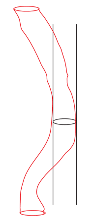
Figure 4. Averaging of the approximation near the middle.

3.3.1. The Averaging Map $\mathsf{A}_{\Phi}$

With $S^{1}={\mathbb{R}}/{\mathbb{Z}}$ we have the canonical periodic orbit $t\rightarrow t$ and its shifts $t\rightarrow t+c$. Consider for the Abelian group $S^{1}$ the standard covering map

$$e:{\mathbb{R}}\rightarrow S^{1}:t\rightarrow t\ \text{mod}\ {\mathbb{Z}}.$$

In the following we shall consider (continuous) maps $q:S^{1}\rightarrow S^{1}$. For such a $q$ take a continuous lift $\widetilde{q}:{\mathbb{R}}\rightarrow{\mathbb{R}}$ which then satisifies

$$e\circ\widetilde{q}(t)=q(e(t))\ \text{for all}\ t\in{\mathbb{R}}.$$

We define

$$\oint_{S^{1}}q(t)\cdot dt:=\int_{[0,1]}\widetilde{q}(t)\cdot dt\ \text{mod}\ {\mathbb{Z}}.$$

The definition does not depend on the choice of the lift. We shall also sometimes refer to this integral as the $S^{1}$-average or $\oint_{S^{1}}$-average of $q$.

Definition 3.37.

With $\bm{{\gamma}}$ being a periodic orbit in ${\mathbb{R}}^{N}$, a good averaging coordinate $\Phi:U\rightarrow S^{1}$ consists of an open neighborhood $U\subset{\mathbb{R}}^{N}$ of $\gamma(S^{1})$ and a smooth map $\Phi:U\rightarrow S^{1}$ such that for a suitable $\gamma_{0}\in[\gamma]$ it holds that $\Phi\circ\gamma_{0}(t)=t$ for $t\in S^{1}$. (Note that $\gamma_{0}$ is uniquely determined by $\Phi$.)

Given $\bm{\gamma}$ and $\Phi:U\rightarrow S^{1}$ assume that $w:Z_{a}\rightarrow{\mathbb{R}}^{N}$ is a continuous map, where $Z_{a}$ is obtained from the gluing parameter $a=|a|\cdot[\widehat{x},\widehat{y}]$ and the ordered disk pair $((D_{x},D_{y}),(x,y))$. Next we need the notion of a ‘middle annulus’ on $Z_{a}$.

Definition 3.38.

Define $M^{h}_{a}$, the so-called middle annulus of $Z_{a}$ of width $2\cdot h$, for $h\in[0,15)$, to consist of all $(z,z^{\prime})\in Z_{a}$ such that $z=\sigma^{+,a}_{\widehat{x}}(s,t)$ with $s\in[R/2-h,R/2+h]$, where $R=\varphi(|a|)$, and $t\in S^{1}$. Since $|a|\in(0,1/4)$ it always holds that $M^{h}_{a}\subset Z_{a}$ provided $h\in[0,25)$. For smaller $|a|$ it contains larger middle annuli. See also Appendix

We impose the following two properties on ${w}:Z_{a}\rightarrow{\mathbb{R}}^{N}$:

• ${w}(M^{3}_{a})\subset U$.

• For a decoration $\widehat{x}$ the map $S^{1}\rightarrow S^{1}:t\rightarrow\Phi\circ w\circ\sigma_{\widehat{x}}^{+,a}(R/2,t)$ has degree $k$. Of course, the degree does not depend on the decoration of $x$.

The $\oint_{S^{1}}$-average of the map in (2) depends on the choice of $\widehat{x}$, but we shall introduce later on new expressions which do not, and which carriy nontrivial information. For this reason we need to understand fully certain dependencies.

Lemma 3.39.

Let $\theta=e^{2\pi i\tau}$ for $\tau\in[0,1)$. Then mod ${\mathbb{Z}}$ we have the identity

$$\oint_{S^{1}}\Phi\circ w\circ\sigma_{\theta\cdot\widehat{x}}^{+,a}(R/2,t)\cdot dt=\oint_{S^{1}}\Phi\circ w\circ\sigma_{\widehat{x}}^{+,a}(R/2,t)\cdot dt-k\tau.$$

Proof.

We note that $\sigma^{+}_{\theta\cdot\widehat{x}}(s,t+\tau)=\sigma_{\widehat{x}}^{+}(s,t)$. We define

$$\alpha(t):=\Phi\circ w\circ\sigma_{\theta\cdot\widehat{x}}^{+,a}(R/2,t)$$

and consequently

$$\alpha(t+\tau)=\Phi\circ w\circ\sigma_{\theta\cdot\widehat{x}}^{+,a}(R/2,t+\tau)=\Phi\circ w\circ\sigma_{\widehat{x}}^{+,a}(R/2,t).$$

Then we compute mod ${\mathbb{Z}}$

$$\oint_{S^{1}}\alpha(t)\cdot dt=\int_{0}^{1}\widetilde{\alpha}(t)\cdot dt\ \ \text{mod}\ \ {\mathbb{Z}}$$

$$= \int_{-\tau}^{1-\tau}\widetilde{\alpha}(t+\tau)\cdot dt\ \ \text{mod}\ \ {\mathbb{Z}}$$

$$= \int_{-\tau}^{0}\widetilde{\alpha}(t+\tau)\cdot dt+\int_{0}^{1-\tau}\widetilde{\alpha}(t+\tau)\cdot dt\ \ \text{mod}\ \ {\mathbb{Z}}$$

$$= \int_{1-\tau}^{1}(\widetilde{\alpha}(t+\tau)-k)\cdot dt+\int_{0}^{1-\tau}\widetilde{\alpha}(t+\tau)\cdot dt\ \ \text{mod}\ \ {\mathbb{Z}}$$

$$= \int_{0}^{1}\widetilde{\alpha}(t+\tau)\cdot dt-k\cdot\tau\ \ \text{mod}\ \ {\mathbb{Z}}$$

$$= \oint_{S^{1}}\alpha(t+\tau)\cdot dt-k\cdot\tau\ \ \text{mod}\ \ {\mathbb{Z}}.$$

∎

Given $\Phi$ there exists a unique $\gamma_{0}$ satisfying $\Phi\circ\gamma_{0}(t)=t$ mod $1$. Every other $\gamma\in[\gamma_{0}]$ can be written as $\gamma(t)=\gamma_{0}(t+c)$ for some $c\in S^{1}$ and we abbreviate $\gamma_{c}(t)=\gamma_{0}(t+c)$ and compute

$$\oint_{S^{1}}\Phi\circ\gamma_{c}(kt)\cdot dt$$

$$= \oint_{S^{1}}\Phi\circ\gamma_{0}(kt+c)=\oint_{S^{1}}(kt+c\ \text{mod}\ {\mathbb{Z}})\cdot dt$$

$$= \int_{0}^{1}(kt+c)\cdot dt\ \text{mod}\ {\mathbb{Z}}=c+k/2\ \text{mod}\ {\mathbb{Z}}.$$

We extend the discussion from the previous Subsection 3.2 to also deal with data of the form $(0,(\widetilde{w}^{x},[\widehat{x},\widehat{y}],\widetilde{w}^{y}))\in\partial\mathfrak{Z}$. Write $\bm{\gamma}=([\gamma],T,k)$.

Definition 3.40.

Having fixed a good averaging coordinate $\Phi:U\rightarrow S^{1}$ for $\bm{\gamma}$, the subset ${\mathcal{W}}$ of $Y^{3,\delta_{0}}_{{\mathcal{D}},\varphi}({\mathbb{R}}\times{\mathbb{R}}^{N},\bm{\gamma})$ consists of the following elements, where as usual $\widetilde{w}=(b,w)$.

• All $(0,(\widetilde{w}^{x},[\widehat{x},\widehat{y}],\widetilde{w}^{y}))$.

• All $(r,\widetilde{w})$ with $r\in(0,1)$ so that $w|M^{3}_{a}$ has the image in $U$ and it holds for a suitable decoration $\widehat{x}$ that for every $s\in[R/2-3,R/2+3]$, $R=R(|a|)=R(|a(\widetilde{w})|)$, the map

  $$S^{1}\rightarrow S^{1}:t\rightarrow\Phi\circ w\circ\sigma^{+,a}_{\widehat{x}}(s,t)$$

  has degree $k$.

Lemma 3.41.

The preimage $\bm{\bar{\oplus}}^{-1}({\mathcal{W}})$ is open in ${\mathcal{V}}$.

Proof.

Obvious. ∎

Assume that $(r,\widetilde{w})\in{\mathcal{W}}$ with $r\in(0,1)$ and write $a=|a|\cdot[\widehat{x},\widehat{y}]$. We pick a representative $(\widehat{x},\widehat{y})\in{\mathbb{S}}_{x}\times{\mathbb{S}}_{y}$ and take the $\oint_{S^{1}}$-average, denoted by $d_{\widehat{x}}(r,\widetilde{w})$

(3.15) $$d_{\widehat{x}}(r,\widetilde{w}):=\oint_{S^{1}}\Phi\circ w\circ\sigma^{+,a}_{\widehat{x}}(R/2,t)\cdot dt\in S^{1},$$

which will depend on $\widehat{x}$ as described in Lemma 3.39. Here $R=\varphi(|a|)$ and $a=|a|\cdot[\widehat{x},\widehat{y}]$. Then we define numbers $c^{x}(r,\widetilde{w})$ and $c^{y}(r,\widetilde{w})$, where $\widetilde{w}=(b,w)$, by

(3.16) $$c^{x}(r,\widetilde{w}):=\int_{S^{1}}b\circ\sigma^{+,a}_{\widehat{x}}(R/2,t)\cdot dt-\frac{1}{2}\cdot T\cdot\varphi(|a|),$$

$$c^{y}(r,\widetilde{w}):=c^{x}(r,\widetilde{w})+T\cdot\varphi(|a|)-\varphi(r)$$

$$\ \ \ \ \ \ \ =\int_{S^{1}}b\circ\sigma^{+,a}_{\widehat{x}}(R/2,t)\cdot dt+\frac{1}{2}\cdot T\cdot\varphi(|a|)-\varphi(r).$$

We note that $d_{\widehat{x}}(r,\widetilde{w})$ depends on the choice of $\widehat{x}$, but that the two real numbers defined in (3.16) do not depend on this choice. Note that at this stage, given $(r,\widetilde{w})\in{\mathcal{W}}$ we can extract from the domain of $\widetilde{w}$ the domain gluing parameter $a=|a|\cdot[\widehat{x},\widehat{y}]$ and the averages as described above. From this data we shall be able to construct some kind of approximation of $\widetilde{w}$ in $\mathsf{S}_{\bm{\gamma}}$.

Lemma 3.42.

Given $(r,\widetilde{w})\in{\mathcal{W}}$ there exists a uniquely determined element $\widetilde{p}:=(\widetilde{p}^{x},[\widehat{x},\widehat{y}],\widetilde{p}^{y})\in\mathsf{S}_{\bm{\gamma}}$ characterized by the following properties, where we write $\widetilde{p}^{x}=(b^{x},p^{x})$ and $\widetilde{p}^{y}=(b^{y},p^{y})$, and $(\widehat{x},\widehat{y})$ is a representative of $[\widehat{x},\widehat{y}]$.

• $c^{x}(\widetilde{p})=c^{x}(r,\widetilde{w})$ and $c^{y}(\widetilde{p})=c^{y}(r,\widetilde{w})$.

• $\oint_{S^{1}}\Phi\circ p^{x}\circ\sigma^{+}_{\widehat{x}}(s,t)\cdot dt=d_{\widehat{x}}(r,\widetilde{w})$ for all $s\in{\mathbb{R}}^{+}$.

• $\oint_{S^{1}}\Phi\circ p^{y}\circ\sigma^{-}_{\widehat{y}}(s^{\prime},t^{\prime})\cdot dt^{\prime}=d_{\widehat{x}}(r,\widetilde{w})$ for all $s^{\prime}\in{\mathbb{R}}^{-}$.

Proof.

We need to prove existence and uniqueness of the element $\widetilde{p}$. Let us note that the expressions in (2) and (3) on the right and left have the same dependencies with respect to $\widehat{x}$ and $\widehat{y}$, respectively, and consequently the equations do not depend on the choices made.

Existence: Denote by $\gamma_{0}\in[\gamma]$ the representative satisfying $\Phi\circ\gamma_{0}(t)=t$ for $t\in S^{1}$. Introduce $\gamma_{c}$ for $c\in S^{1}$ by $\gamma_{c}(t)=\gamma_{0}(t+c)$. Define $\widetilde{p}^{x}=(b^{x},p^{x})$ and $\widetilde{p}^{y}=(b^{y},p^{y})$ by

(3.17) $$\ \ \ \ \ \ b^{x}\circ\sigma_{\widehat{x}}^{+}(s,t)=Ts+c^{x}(r,\widetilde{w}),\ \ b^{y}\circ\sigma_{\widehat{y}}^{-}(s^{\prime},t^{\prime})=Ts^{\prime}+c^{y}(r,\widetilde{w})$$

and

(3.18) $$p^{x}\circ\sigma^{+}_{\widehat{x}}(s,t) = \gamma_{[d_{\widehat{x}}(r,\widetilde{w})-(k/2)]}(kt)$$

$$p^{y}\circ\sigma^{-}_{\widehat{y}}(s^{\prime},t^{\prime}) = \gamma_{[d_{\widehat{x}}(r,\widetilde{w})-(k/2)]}(kt^{\prime}).$$

With these definitions the element $\widetilde{p}=(\widetilde{p}^{x},[\widehat{x},\widehat{y}],\widetilde{p}^{y})$ in fact belongs to $\mathsf{S}_{\bm{\gamma}}$. Namely the $\widehat{x}$-directional limit of $p^{x}\circ\sigma^{+}_{\widehat{x}}(s,t)$ is given by

$$\text{lim}_{s\rightarrow\infty}p^{x}\circ\sigma^{+}_{\widehat{x}}(s,0)=\gamma_{0}(d_{\widehat{x}}(r,\widetilde{w})-k/2)$$

and for $p^{y}$ the $\widehat{y}$-directional limit by

$$\text{lim}_{s^{\prime}\rightarrow-\infty}p^{y}\circ\sigma^{-}_{\widehat{y}}(s^{\prime},0)=\gamma_{0}(d_{\widehat{x}}(r,\widetilde{w})-k/2).$$

Hence the data is $[\widehat{x},\widehat{y}]$-matching. The real asymptotic constants satisfy

$$c^{x}(\widetilde{p})=c^{x}(r,\widetilde{w})\ \text{and}\ c^{y}(\widetilde{p})=c^{y}(r,\widetilde{w}).$$

We compute

$$\oint_{S^{1}}\Phi\circ p^{x}\circ\sigma_{\widehat{x}}^{+}(s,t)\cdot dt=(\int_{0}^{1}[kt+d_{\widehat{x}}(r,\widetilde{w})-(k/2)]\cdot dt)_{/{\mathbb{Z}}}=d_{\widehat{x}}(r,\widetilde{w})$$

and similarly

$$\oint_{S^{1}}\Phi\circ p^{y}\circ\sigma_{\widehat{y}}^{+}(s^{\prime},t^{\prime})\cdot dt^{\prime}=d_{\widehat{x}}(r,\widetilde{w}).$$

Uniqueness: Assume that $\widetilde{p}_{1}$ is another element in $\mathsf{S}_{\bm{\gamma}}$ and $[\widehat{x}_{1},\widehat{y}_{1}]=[\widehat{x},\widehat{y}]$ such that

$$c^{x}(\widetilde{p}_{1})=c^{x}(r,\widetilde{w})\ \text{and}\ \ c^{y}(\widetilde{p}_{1})=c^{y}(r,\widetilde{w})$$

and

(3.19) $$\oint_{S^{1}}\Phi\circ p^{x}_{1}\circ\sigma_{\widehat{x}_{1}}^{+}(s,t)\cdot dt=d_{\widehat{x}_{1}}(r,\widetilde{w})$$

$$\oint_{S^{1}}\Phi\circ p^{y}_{1}\circ\sigma_{\widehat{y}_{1}}^{-}(s^{\prime},t^{\prime})\cdot dt^{\prime}=d_{\widehat{x}_{1}}(r,\widetilde{w}).$$

Then $c^{x}(\widetilde{p})=c^{x}(\widetilde{p}_{1})$ and $c^{y}(\widetilde{p})=c^{y}(\widetilde{p}_{1})$. We can write

$$p_{1}^{x}\circ\sigma_{\widehat{x}_{1}}^{+}(s,t)=\gamma_{0}(kt+c)$$

for a suitable $c\in[0,1)$ and similarly $p^{x}\circ\sigma_{\widehat{x}}^{+}(s,t)=\gamma_{0}(kt+c_{0})$. We compute (mod ${\mathbb{Z}}$) with $\theta=e^{2\pi i\tau}$, $\tau\in[0,1)$, and $\widehat{x}_{1}=\theta\cdot\widehat{x}$ and $\widehat{y}_{1}=\theta^{-1}\cdot\widehat{y}$ the following

$$k/2+c\ \text{mod}\ {\mathbb{Z}}=\oint_{S^{1}}(kt+c\ \text{mod}\ \ {\mathbb{Z}})\cdot dt$$

$$= \oint_{S^{1}}\Phi\circ p^{x}_{1}\circ\sigma_{\widehat{x}_{1}}^{+}(s,t)\cdot dt$$

$$= d_{\widehat{x}_{1}}(r,\widetilde{w})=d_{\widehat{x}}(r,\widetilde{w})-k\tau\ \text{mod}\ {\mathbb{Z}}$$

$$= \oint_{S^{1}}\Phi\circ p^{x}\circ\sigma_{\widehat{x}}^{+}(s,t)\cdot dt-k\tau\ \text{mod}\ {\mathbb{Z}}$$

$$= \oint_{S^{1}}(kt+c_{0}\ \text{mod}\ {\mathbb{Z}})\cdot dt-k\tau\ \text{mod}\ {\mathbb{Z}}$$

$$= k/2+c_{0}-k\tau\ \text{mod}\ {\mathbb{Z}}.$$

Consequently $c=c_{0}-k\tau$ mod ${\mathbb{Z}}$. Hence

$$p^{x}_{1}\circ\sigma^{+}_{\widehat{x}_{1}}(s,t)=\gamma_{0}(kt+c)$$

$$= \gamma_{0}(kt+c_{0}-k\tau)=\gamma_{0}(k(t-\tau)+c_{0})$$

$$= p^{x}\circ\sigma^{+}_{\widehat{x}}(s,t-\tau)=p^{x}\circ\sigma^{+}_{\widehat{x}_{1}}(s,t).$$

This shows that $p^{x}_{1}=p^{x}$ and similarly we can show that $p^{y}_{1}=p^{y}$. This completes the proof of uniqueness. ∎

In view of this lemma we can now give the definition of the averaging map $\mathsf{A}_{\Phi}$.

Definition 3.43.

Given a good averaging coordinate $\Phi:U\rightarrow S^{1}$ associated to $\bm{\gamma}$ the averaging map

$$\mathsf{A}_{\Phi}:{\mathcal{W}}\rightarrow\mathsf{S}_{\bm{\gamma}}$$

is defined as follows. For the special elements with $r=0$ we set

$$\mathsf{A}_{\Phi}(0,(\widetilde{q}^{x},[\widehat{x},\widehat{y}],\widetilde{q}^{y})\dotplus(\widetilde{h}^{x},\widetilde{h}^{y}))=(\widetilde{q}^{x},[\widehat{x},\widehat{y}],\widetilde{q}^{y})$$

For elements $(r,\widetilde{w})$ with $r\neq 0$ we define

$$\mathsf{A}(r,\widetilde{w})=\widetilde{p},$$

with $c^{x}(\widetilde{p})=c^{x}(r,\widetilde{w})$, $c^{y}(\widetilde{p})=c^{y}(r,\widetilde{w})$ and

$$d_{\widehat{x}}(r,\widetilde{w})=\oint_{S^{1}}\Phi\circ p^{x}\circ\sigma^{+}_{\widehat{x}}(s,t)\cdot dt=\oint_{S^{1}}\Phi\circ p^{y}\circ\sigma^{+}_{\widehat{y}}(s^{\prime},t^{\prime})\cdot dt^{\prime}.$$

Remark 3.44.

$A_{\Phi}(r,\widetilde{w})$ gives an element $\widetilde{p}=(\widetilde{p}^{x},[\widehat{x},\widehat{y}],\widetilde{p}^{y})$ in $\mathsf{S}_{\gamma}$, so that the map $\bar{\oplus}(r,(\widetilde{p}^{x},[\widehat{x},\widehat{y}],\widetilde{p}^{y}))$, is in some sense the best approximation of $\widetilde{w}$ by a simple type of maps.

Exercise 9.

Prove for $(r,\widetilde{q})\in[0,1)\times\mathsf{S}_{\bm{\gamma}}$ the identity

$$\widetilde{q}=\mathsf{A}_{\Phi}\circ\bm{\bar{\oplus}}(r,\widetilde{q}).$$

At this point, as the basic achievement of this subsection, we have constructed the averaging map $\mathsf{A}_{\Phi}$.

3.3.2. Sc-Smoothness Properties of $\mathsf{A}_{\Phi}$

The main goal of this subsection is the study of the sc-smoothness properties of $\mathsf{A}_{\Phi}$. To begin our considerations define the smooth manifold

$$\mathsf{M}={\mathbb{R}}\times{\mathbb{S}}_{{\mathcal{D}}}\times S^{1}\times{\mathbb{R}}.$$

Here ${\mathbb{S}}_{\mathcal{D}}$ is the smooth manifold diffeomorphic to ${\mathbb{S}}^{1}$ consisting of the set of all $[\widehat{x},\widehat{y}]$. We fix $\widehat{x}_{0}$ so that every element $[\widehat{x}^{\prime},\widehat{y}^{\prime}]\in{\mathbb{S}}_{{\mathcal{D}}}$ can be uniquely written as $[\widehat{x}_{0},\widehat{y}]$. Associated to this choice $\widehat{x}_{0}$ we define a map

$$\mathsf{R}_{\widehat{x}_{0}}:\mathsf{M}\rightarrow\mathsf{S}_{\bm{\gamma}}$$

by associating to $(c^{x},[\widehat{x}_{0},\widehat{y}],d,c^{y})$ the element

$$\widetilde{p}:=\mathsf{R}_{\widehat{x}_{0}}(c^{x},[\widehat{x}_{0},\widehat{y}],d,c^{y}),$$

defined by $\widetilde{p}=(\widetilde{p}^{x},[\widehat{x}_{0},\widehat{y}],\widetilde{p}^{y})$ satisfying with $\widetilde{p}^{x}=(b^{x},p^{x})$ and $\widetilde{p}^{y}=(b^{y},p^{y})$

$$b^{x}\circ\sigma^{+}_{\widehat{x}_{0}}(s,t)=Ts+c^{x}\ \text{and}\ \ b^{y}\circ\sigma^{-}_{\widehat{y}}(s^{\prime},t^{\prime})=Ts^{\prime}+c^{y}$$

and moreover

$$\oint_{S^{1}}\Phi\circ p^{x}\circ\sigma^{+}_{\widehat{x}_{0}}(s,t)\cdot dt=d\ \ \text{and}\ \ \oint_{S^{1}}\Phi\circ p^{y}\circ\sigma^{-}_{\widehat{y}}(s^{\prime},t^{\prime})\cdot dt^{\prime}=d.$$

Lemma 3.45.

The map $\mathsf{R}_{\widehat{x}_{0}}$ is smooth.

Proof.

Recall that $\Phi\circ\gamma_{0}(t)=t$. We define for $d\in S^{1}$ the element $p^{x}_{d}$ by

$$p^{x}_{d}\circ\sigma_{\widehat{x}_{0}}(s,t)=\gamma_{0}(kt-(k/2)+d),$$

so that $\oint_{S^{1}}\Phi\circ p^{x}_{d}\circ\sigma_{\widehat{x}_{0}}(s,t)\cdot dt=d$. We define $b^{x}_{c^{x}}$ by $b^{x}_{c^{x}}\circ\sigma^{+}_{\widehat{x}_{0}}(s,t)=Ts+c^{x}$ and $b^{y}_{c^{y}}$ by $b^{y}_{c^{y}}\circ\sigma^{-}_{\widehat{y}}(s^{\prime},t^{\prime})=Ts^{\prime}+c^{y}$. We note that the definition of the latter does not depend on the choice of $\widehat{y}$. The element $p^{y}_{\widehat{y},d}$ is defined by

$$p^{y}_{\widehat{y},d}\circ\sigma^{-}_{\widehat{y}}(s^{\prime},t^{\prime})=\gamma_{0}(kt^{\prime}-(k/2)+d).$$

With these definitions it follows that

$$\mathsf{R}_{\widehat{x}_{0}}(c^{x},[\widehat{x}_{0},\widehat{y}],d,c^{y})=((b^{x}_{c^{x}},p^{x}_{d}),[\widehat{x}_{0},\widehat{y}],(b^{y}_{c^{y}},p^{y}_{d,\widehat{y}})).$$

We recall the maps $\phi_{\gamma}$ defined in (3.5) which are smooth $k:1$ coverings. We note that

$$\phi_{\gamma_{0}}(c^{x},e^{-2\pi i(d-k/2)}\cdot\widehat{x}_{0},c^{y},e^{2\pi i(d-k/2)}\cdot\widehat{y})=\mathsf{R}_{\widehat{x}_{0}}(c^{x},[\widehat{x}_{0},\widehat{y}],d,c^{y}),$$

and the smoothness of the map

$$(c^{x},[\widehat{x}_{0},\widehat{y}],d,c^{y})\rightarrow(c^{x},e^{-2\pi i(d-k/2)}\cdot\widehat{x}_{0},c^{y},e^{2\pi i(d-k/2)}\cdot\widehat{y})$$

implies the desired result since $\phi_{\gamma_{0}}$ is a local diffeomorphism. ∎

Our aim is to show that $\bm{\bar{\oplus}}:{\mathcal{V}}\rightarrow Y^{3,\delta_{0}}_{{\mathcal{D}},\varphi}$ is an $\oplus$-polyfold construction and defines a M-polyfold structure on the target characterized by a list of properties. Since ${\mathcal{W}}$ is a subset of $Y^{3,\delta_{0}}_{{\mathcal{D}},\varphi}$ which is open for the quotient topology ${\mathcal{T}}$, the sc-smoothnees of $\mathsf{A}_{\Phi}$ for the M-polyfold structure would be equivalent to the sc-smoothness of the map $A_{\Phi}\circ\bm{\bar{\oplus}}:\bm{\bar{\oplus}}^{-1}({\mathcal{W}})\rightarrow\mathsf{S}_{\bm{\gamma}}$, if in fact $\bm{\bar{\oplus}}$ defines a M-polyfold structure. In view of the previous lemma we can reduce this question to the study of the dependencies of $c^{x},c^{y}$ and $d$. The following result means that $\mathsf{A}_{\Phi}$ will be sc-smooth for the M-polyfold structure we are going to define on $Y^{3,\delta_{0}}_{{\mathcal{D}},\varphi}$.

Proposition 3.46.

The map

$$\mathsf{A}_{\Phi}\circ\bm{\bar{\oplus}}:\bm{\bar{\oplus}}^{-1}({\mathcal{W}})\rightarrow\mathsf{S}_{\bm{\gamma}},$$

which is defined on an open subset of ${\mathcal{V}}$ containing $\partial\mathfrak{Z}$, is sc-smooth.

Proof.

Given an element $(r,(\widetilde{u}^{x},[\widehat{x},\widehat{y}],\widetilde{u}^{y}))\in\bm{\bar{\oplus}}^{-1}({\mathcal{W}})$ we define

$$\widetilde{w}=\bm{\bar{\oplus}}(r,(\widetilde{u}^{x},[\widehat{x},\widehat{y}],\widetilde{u}^{y})),$$

where, if $r=0$, $\widetilde{w}$ stands for $(0,(\widetilde{u}^{x},[\widehat{x},\widehat{y}],\widetilde{u}^{y}))$. The procedure produces from $[\widehat{x},\widehat{y}]$, if $r\neq 0$ a glued surface $Z_{a}$ on which $\widetilde{w}$ is defined, where $a$ has angular part $[\widehat{x},\widehat{y}]$ and in the case $r=0$ keeps it as part of the data. The element $(\widetilde{u}^{x},[\widehat{x},\widehat{y}],\widetilde{u}^{y})$ has the form

$$\widetilde{q}\dotplus\widetilde{h}:=(\widetilde{q}^{x},[\widehat{x},\widehat{y}],\widetilde{q}^{y})\dotplus(\widetilde{h}^{x},\widetilde{h}^{y})$$

and the gluing parameter $a$ is smoothly computed from $(r,\widetilde{q})\in[0,1)\times\mathsf{S}_{\bm{\gamma}}$. Consider $\widetilde{Q}:=\bm{\bar{\oplus}}(r,(\widetilde{q}^{x},[\widehat{x},\widehat{y}],\widetilde{q}^{y}))$, which equals $(\widetilde{q}^{x},[\widehat{x},\widehat{y}],\widetilde{q}^{y})$ if $r=0$ and $\widetilde{H}=\oplus_{a}(\widetilde{h}^{x},\widetilde{h}^{y})$, where $a=\mathsf{a}(r,(\widetilde{u}^{x},[\widehat{x},\widehat{y}],\widetilde{u}^{y}))$ is the associated gluing parameter, which by Lemma 3.18 is ssc-smooth. Then

$$\bm{\bar{\oplus}}(r,(\widetilde{u}^{x},[\widehat{x},\widehat{y}],\widetilde{u}^{y}))=\bm{\bar{\oplus}}(r,(\widetilde{q}^{x},[\widehat{x},\widehat{y}],\widetilde{q}^{y}))+\oplus_{a}(\widetilde{h}^{x},\widetilde{h}^{y})=\widetilde{Q}+\widetilde{H}.$$

Write $\widetilde{Q}=(B,Q)$ and $\widetilde{H}=(C,H)$ and fix a decoration $\widehat{x}_{0}$. With the definitions in (3.15) and (3.16) we obtain using $R=\varphi(|a|)$

$$c^{x}(r,\widetilde{w})=\int_{S^{1}}[B\circ\sigma^{+}_{\widehat{x}_{0}}(R/2)+C\circ\sigma^{+}_{\widehat{x}_{0}}(R/2,t)]\cdot dt-\frac{1}{2}\cdot T\cdot R$$

$$= c^{x}(\widetilde{q}^{x})+\int_{S^{1}}C\circ\sigma^{+}_{\widehat{x}_{0}}(R/2,t)\cdot dt.$$

Here we have used that $\widetilde{Q}$ is the restriction of $\widetilde{q}^{x}$ to $Z_{a}$. Given $[\widehat{x},\widehat{y}]$ there exists a smooth map $[\widehat{x},\widehat{y}]\rightarrow\widehat{y}_{0}([\widehat{x},\widehat{y}])$ such that

$$[\widehat{x},\widehat{y}]=[\widehat{x}_{0},\widehat{y}_{0}([\widehat{x},\widehat{y}])].$$

Next we compute, abbreviating $\widehat{y}_{0}=\widehat{y}_{0}([\widehat{x},\widehat{y}])$

$$c^{y}(r,\widetilde{w})=c^{x}(\widetilde{q}^{x})+T\cdot R-\varphi(r)+\int_{S^{1}}C\circ\sigma^{+}_{\widehat{x}_{0}}(R/2,t)\cdot dt$$

$$= c^{y}(\widetilde{q}^{y})+\int_{S^{1}}C\circ\sigma^{+}_{\widehat{x}_{0}}(R/2,t)\cdot dt.$$

Further we compute

(3.22) $$d_{\widehat{x}_{0}}(r,\widetilde{w})=\oint_{S^{1}}\Phi\circ(Q+H)\circ\sigma^{+,a}_{\widehat{x}_{0}}(R/2,t)\cdot dt.$$

In view of Lemma 3.45 it suffices to show that the maps

$$(r,\widetilde{q}\dotplus\widetilde{h})\rightarrow\widehat{y}_{0}([\widehat{x},\widehat{y}])$$

$$(r,\widetilde{q}\dotplus\widetilde{h})\rightarrow c^{x}(r,\widetilde{w})$$

$$(r,\widetilde{q}\dotplus\widetilde{h})\rightarrow c^{y}(r,\widetilde{w})$$

$$(r,\widetilde{q}\dotplus\widetilde{h})\rightarrow d_{\widehat{x}_{0}}(r,\widetilde{w}).$$

are sc-smooth. As a consequence of our discussion so far this boils down to the sc-moothness of the following maps, where we use smoothness properties of $c^{x}(\widetilde{q}^{x})$ and $c^{y}(\widetilde{q}^{y})$.

(3.23) $$(r,\widetilde{q}\dotplus\widetilde{h})\rightarrow\widehat{y}_{0}([\widehat{x},\widehat{y}])$$

(3.24) $$(r,\widetilde{q}\dotplus\widetilde{h})\rightarrow\int_{S^{1}}C\circ\sigma^{+}_{\widehat{x}_{0}}(R/2,t)\cdot dt$$

(3.25) $$(r,\widetilde{q}\dotplus\widetilde{h})\rightarrow d_{\widehat{x}_{0}}(r,\widetilde{w})$$ .

The first map (3.23) is ssc-smooth. The second map (3.24) has, with $\widetilde{h}^{x}=(b^{x},h^{x})$ and $\widetilde{h}^{y}=(b^{y},h^{y})$ the form

$$(r,\widetilde{q}\dotplus\widetilde{h})\rightarrow\int_{S^{1}}\frac{1}{2}\cdot[b^{x}(R/2,t)+b^{y}(R/2,t)]\cdot dt$$

and is sc-smooth (not ssc-smooth!) by the definition of the ssc-structure on $Z_{\mathcal{D}}({\mathbb{R}}\times{\mathbb{R}}^{N},\bm{\bar{\gamma}})$, see Proposition 3.8 and before and Lemma 3.18, for which the map $(r,\widetilde{q}\dotplus\widetilde{h})\rightarrow(\mathsf{a}(r,\widetilde{q}),\widetilde{h})$ is ssc-smooth, and the Fundamental Lemma in Subsection 1.2. It remains to show that the third map (3.25) is sc-smooth. We shall write the map $(r,\widetilde{q}\dotplus\widetilde{h})\rightarrow d_{\widehat{x}_{0}}(r,\widetilde{w})$ more explicitly. For this note that

$$w\circ\sigma_{\widehat{x}_{0}}(R/2,t)$$

$$+\frac{1}{2}\cdot[h^{x}\circ\sigma^{+}_{\widehat{x}_{0}}(R/2,t)+h^{y}\circ\sigma^{-}_{\widehat{y}_{0}([\widehat{x},\widehat{y}])}(-R/2,t)]$$

$$= \gamma_{0}(kt+m(\widetilde{q}))$$

$$+\frac{1}{2}\cdot[h^{x}\circ\sigma^{+}_{\widehat{x}_{0}}(R/2,t)+h^{y}\circ\sigma^{-}_{\widehat{y}_{oo}}(-R/2,t+\vartheta([\widehat{x},\widehat{y}]))],$$

where $q^{+}\circ\sigma^{+}_{\widehat{x}_{0}}(s,t)=\gamma_{0}(m(\widetilde{q})+kt)$, $\widehat{y}_{oo}$ is a fixed choice so that

$$\sigma^{-}_{\widehat{y}_{oo}}(s^{\prime},t^{\prime}+\vartheta([\widehat{x},\widehat{y}]))=\sigma^{-}_{\widehat{y}_{0}([\widehat{x},\widehat{y}])}(s^{\prime},t^{\prime}).$$

We note that $m(\widetilde{q})$ and $\vartheta([\widehat{x},\widehat{y}])$ depend ssc-smoothly on $(r,\widetilde{q}+\widetilde{h})$. In view of the Fundamental Lemma the map

$${\mathbb{B}}\times H^{3,\delta}({\mathbb{R}}^{+}\times S^{1},{\mathbb{R}}^{N})\rightarrow H^{3,\delta}({\mathbb{R}}^{+}\times S^{1},{\mathbb{R}}^{N}):$$

$$(a,h\circ\sigma^{+}_{\widehat{x}_{0}})\rightarrow h\circ\sigma^{+}_{\widehat{x}_{0}}(R/2+s,t)$$

is sc-smooth. Similarly

$${\mathbb{B}}\times H^{3,\delta}({\mathbb{R}}^{-}\times S^{1},{\mathbb{R}}^{N})\rightarrow H^{3,\delta}({\mathbb{R}}^{-}\times S^{1},{\mathbb{R}}^{N}):$$

$$(a,h\circ\sigma^{-}_{\widehat{y}_{oo}})\rightarrow h\circ\sigma^{-}_{\widehat{y}_{oo}}(-R/2+s,t-\theta).$$

In the above definition, in the case $a=0$ the image is the zero-map. We also note that the maps $H^{3,\delta}({\mathbb{R}}^{\pm}\times S^{1},{\mathbb{R}}^{N})\rightarrow C^{0}(S^{1},{\mathbb{R}}^{N})$

$$h^{\pm}\rightarrow h^{\pm}(0,.),$$

where $C^{0}$ is equipped with the standard sc-structure, i.e. level $m$ corresponds to $C^{m}$, are linear sc-operators. The map

$$S^{1}\times C^{0}(S^{1},{\mathbb{R}}^{N})\rightarrow C^{0}(S^{1},{\mathbb{R}}^{N}):(e,\sigma)\rightarrow[t\rightarrow\sigma(t+e)]$$

is sc-smooth which is an easy exercise along the line of similar results in [38]. Revisiting (3.3.2) we deduce from the previous discussion the following facts.

Fact 3.47.

The following maps $\bm{\bar{\oplus}}^{-1}({\mathcal{W}})\rightarrow C^{0}(S^{1},{\mathbb{R}}^{N})$ are sc-smooth.

• $(r,\widetilde{q}\dotplus\widetilde{h})\rightarrow[t\rightarrow\gamma_{0}(t+m(\widetilde{q}))]$.

• $(r,\widetilde{q}\dotplus\widetilde{h})\rightarrow[t\rightarrow h^{x}\circ\sigma^{+}_{\widehat{x}_{0}}(R/2,t)].$

• $(r,\widetilde{q}\dotplus\widetilde{h})\rightarrow h^{y}\circ\sigma^{-}_{\widehat{y}_{oo}}([\widehat{x},\widehat{y}])(-R/2,t+\vartheta([\widehat{x},\widehat{y}]))]$.

As a consequence the map

$$\bm{\bar{\oplus}}^{-1}({\mathcal{W}})\rightarrow C^{0}(S^{1},{\mathbb{R}}^{N}):(r,\widetilde{q}+\widetilde{h})\rightarrow[t\rightarrow w\circ\sigma_{\widehat{x}_{0}}(R/2,t)]$$

is sc-smooth and takes image in $C^{0}(S^{1},U)$. The map $C^{0}(S^{1},U)\rightarrow C^{0}(S^{1},S^{1})$ defined by

$$u\rightarrow\Phi\circ u$$

is ssc-smooth. From this we obtain that

$$\bm{\bar{\oplus}}^{-1}({\mathcal{W}})\rightarrow C^{0}(S^{1},S^{1}):(r,\widetilde{q}\dotplus\widetilde{h})\rightarrow[t\rightarrow\Phi\circ w\circ\sigma_{\widehat{x}_{0}}(R/2,t)]$$

is sc-smooth and by construction takes the values in the maps of degree $k$. Taking the $\oint$-average is obviously sc-smooth. Hence we see that we can write the map

$$(r,\widetilde{q}\dotplus\widetilde{h})\rightarrow d_{\widehat{x}_{0}}(r,\widetilde{w})$$

as a composition of sc-smooth and ssc-smooth maps and consequently by the chain rule this map is sc-smooth. The proof of the proposition is complete. ∎

The result of this subsection can be summarized as follows.

3.4. Comparing Averages

The main goal of this subsection is to understand quantitatively the average. Namely starting with $(r,q\dotplus\widetilde{h})$ we can compare $\widetilde{q}$ and $\widetilde{p}=\mathsf{A}_{\Phi}\circ\bm{\bar{\oplus}}(r,\widetilde{q}\dotplus\widetilde{h})$, where we recall that $\widetilde{q}=\mathsf{A}_{\Phi}\circ\bm{\bar{\oplus}}(r,\widetilde{q})$. The main result in this subsection is Proposition 3.48 and this result will be crucial to define the (second) map $K$ which partially inverts $\bm{\bar{\oplus}}$ in the (next) Subsection 3.5.

We shall use some facts which were derived in the proof of the previous Proposition 3.46. Abbreviate ${\mathcal{U}}=\bm{\bar{\oplus}}^{-1}({\mathcal{W}})$ and consider the sc-smooth map

$$\mathsf{A}_{\Phi}\circ\bm{\bar{\oplus}}:{\mathcal{U}}\rightarrow\mathsf{S}_{\bm{\gamma}},$$

where $\mathsf{A}_{\Phi}$ is introduced in Definition 3.43. A given element in ${\mathcal{U}}$

$$(r,(\widetilde{u}^{x},[\widehat{x},\widehat{y}],\widetilde{u}^{y}))$$

can be written uniquely as

$$(r,(\widetilde{u}^{x},[\widehat{x},\widehat{y}],\widetilde{u}^{y}))=(r,\widetilde{q}\dotplus\widetilde{h}),$$

where $\widetilde{q}=(\widetilde{q}^{x},[\widehat{x},\widehat{y}],\widetilde{q}^{y})\in\mathsf{S}_{\bm{\gamma}}$ and $\widetilde{h}=(\widetilde{h}^{x},\widetilde{h}^{y})$ has the usual decay properties. We denote by $a=\mathsf{a}(r,\widetilde{q})$ the associated gluing parameter, which we recall does not depend on $\widetilde{h}$, and abbreviate $\widetilde{p}=\mathsf{A}_{\Phi}\circ\bm{\bar{\oplus}}(r,\widetilde{q}\dotplus\widetilde{h})$. We define the map

$$\mathsf{D}:{\mathcal{U}}\rightarrow H^{3,\delta}({\mathcal{D}},{\mathbb{R}}\times{\mathbb{R}}^{N})$$

as follows

(3.29) $$\ \ \ \ \ \ \ \mathsf{D}(r,\widetilde{q}\dotplus\widetilde{h})=\left[\begin{array}[]{cc}(\beta^{x}_{a,-2}\cdot(\widetilde{q}^{x}-\widetilde{p}^{x}),\beta^{y}_{a,-2}\cdot(\widetilde{q}^{y}-\widetilde{p}^{y}))&r\neq 0\\ (0,0)&r=0.\end{array}\right.$$

From the discussion in the previous subsection it is clear that the map $\mathsf{D}$ is sc-smooth when we restrict it to $\dot{\mathcal{U}}=\{(r,\widetilde{q}\dotplus\widetilde{h})\in{\mathcal{U}}\ |\ r\neq 0\}$. However, the case near $r=0$ is subtle. If $(r,\widetilde{q}\dotplus\widetilde{h})$ converges to $(0,\widetilde{q}_{0}\dotplus\widetilde{h}_{0})$ one needs to show that the average $\widetilde{p}$ converges to $\widetilde{q}$ fast enough, so that cutting-off their difference (with cut-off functions of increasing support), the resulting map is sc-smooth, see (3.29). Here is the precise statement.

Proposition 3.48.

The map $\mathsf{D}:{\mathcal{U}}\rightarrow H^{3,\delta}({\mathcal{D}},{\mathbb{R}}\times{\mathbb{R}}^{N})$ is sc-smooth.

The proof will follow from two lemmata. Abbreviate $\widetilde{k}=\mathsf{D}(r,\widetilde{q}\dotplus\widetilde{h})$ and

(3.30) $$\widetilde{k}=(\widetilde{k}^{x},\widetilde{k}^{y})\ \ \text{and}\ \ \widetilde{k}^{x}=(e^{x},k^{x}),\ \widetilde{k}^{y}=(e^{y},k^{y}).$$

Lemma 3.49.

The map ${\mathcal{U}}\rightarrow H^{3,\delta}({\mathcal{D}},{\mathbb{R}}):(r,\widetilde{q}\dotplus\widetilde{h})\rightarrow(e^{x},e^{y})$ is sc-smooth.

Proof.

It suffices to study the problem near an element with $r=0$. From the definition of $\widetilde{p}$, using (3.3.2) and (3.3.2) it follows that

$$c^{x}(\widetilde{q})-c^{x}(\widetilde{p})$$

$$= c^{y}(\widetilde{q})-c^{y}(\widetilde{p})$$

$$= -\frac{1}{2}\cdot\int_{S^{1}}[b^{x}\circ\sigma^{+}_{\widehat{x}}(R/2,t)+b^{y}\circ\sigma^{-}_{\widehat{y}}(-R/2,t)]\cdot dt,$$

where $\widetilde{h}^{x}=(b^{x},h^{x})$ and $\widetilde{h}^{y}=(b^{y},h^{y})$ and $\widetilde{h}=(\widetilde{h}^{x},\widetilde{h}^{y})$. We note that the choice of $(\widehat{x},\widehat{y})$ is indeed irrelevant. Writing $\widetilde{k}=\mathsf{D}(r,\widetilde{q}\dotplus\widetilde{h})$ the first component $e^{x}$ of $\widetilde{k}^{x}$ is given by

$$e^{x}\circ\sigma^{+}_{\widehat{x}_{0}}(s,t)$$

$$= -\frac{1}{2}\cdot\beta(s-R/2-2)\cdot\int_{S^{1}}[b^{x}\circ\sigma^{+}_{\widehat{x}}(R/2,t)+b^{y}\circ\sigma^{-}_{\widehat{y}}(-R/2,t)].$$

Here $b^{x}$ and $b^{y}$ are the first components of $\widetilde{h}^{x}$ and $\widetilde{h}^{y}$, respectively. There is a similar formula for $e^{y}$ and in view of the Fundamental Lemma, see Subsection 1.2, the map

$${\mathcal{U}}\rightarrow H^{3,\delta}({\mathcal{D}},{\mathbb{R}}):(r,\widetilde{q}\dotplus\widetilde{h})\rightarrow(e^{x},e^{y})$$

is sc-smooth. This completes the proof of the lemma. ∎

In order to consider the pair $(k^{x},k^{y})$, see (3.30), we find appropriate formulae for them. Denote by $\gamma_{0}$ the representative satisfying $\Phi\circ\gamma_{0}(t)=t$. Then

$$k^{x}\circ\sigma^{+}_{\widehat{x}_{0}}(s,t)$$

$$= \beta(s-R/2-2)\cdot(q^{x}-p^{x})\circ\sigma_{\widehat{x}_{0}}^{+}(s,t)$$

$$= \beta(s-R/2-2)\cdot\left[\gamma_{0}(kt-(k/2)+d_{\widehat{x}_{0}}(\widetilde{q}^{x}))\right.$$

$$\ \ \ \ \ \ \ \ \ \ -\left.\gamma_{0}(kt-(k/2)+d_{\widehat{x}_{0}}(\widetilde{p}^{x}))\right].$$

Similarly

$$k^{y}\circ\sigma^{-}_{\widehat{y}}(s^{\prime},t^{\prime})$$

$$= \beta(|s^{\prime}|-R/2-2)\cdot(q^{y}-p^{y})\circ\sigma_{\widehat{y}}^{-}(s^{\prime},t^{\prime})$$

$$= \beta(|s^{\prime}|-R/2-2)\cdot\left[\gamma_{0}(kt^{\prime}-(k/2)+d_{\widehat{x}_{0}}(\widetilde{q}^{x}))\right.$$

$$\ \ \ \ \ \ \ \ \ \ -\left.\gamma_{0}(kt^{\prime}-(k/2)+d_{\widehat{x}_{0}}(\widetilde{p}^{x}))\right].$$

Here $d_{\widehat{x}_{0}}(\widetilde{q}^{x})=\oint_{S^{1}}\Phi\circ q^{x}\circ\sigma^{+}_{\widehat{x}_{0}}(s,t)\cdot dt$, $(r,\widetilde{w})=\bm{\bar{\oplus}}(r,\widetilde{q}\dotplus\widetilde{h})$, $\widetilde{p}=\mathsf{A}_{\Phi}(r,\widetilde{w})$, and

$$d_{\widehat{x}_{0}}(\widetilde{p}^{x}) = d_{\widehat{x}_{0}}(r,\widetilde{w})$$

$$= \oint_{S^{1}}\Phi\circ w\circ\sigma_{\widehat{x}_{0}}(R/2,t)\cdot dt$$

$$= \oint_{S^{1}}\Phi\circ\left[\gamma_{0}\left(kt-(k/2)+d_{\widehat{x}_{0}}(\widetilde{q}^{x})\right)\phantom{\frac{1}{2}}\right.$$

$$\left.+\frac{1}{2}\cdot\left(h^{x}\circ\sigma^{+}_{\widehat{x}_{0}}(R/2,t)+h^{y}\circ\sigma^{-}_{\widehat{y}}(-R/2,t)\right)\right]\cdot dt.$$

There is a similar formula for the $y$-part. Consequently

$$d_{\widehat{x}_{0}}(\widetilde{p}^{x})-d_{\widehat{x}_{0}}(\widetilde{q}^{x})$$

$$= \oint_{S^{1}}\Phi\circ\left[\gamma_{0}\left(kt-(k/2)+d_{\widehat{x}_{0}}(\widetilde{q}^{x})\right)\phantom{\frac{1}{2}}\right.$$

$$\left.+\frac{1}{2}\cdot\left(h^{x}\circ\sigma^{+}_{\widehat{x}_{0}}(R/2,t)+h^{y}\circ\sigma^{-}_{\widehat{y}}(-R/2,t)\right)\right]\cdot dt$$

$$-\oint_{S^{1}}\Phi\circ\gamma_{0}\left(kt-(k/2)+d_{\widehat{x}_{0}}(\widetilde{q}^{x})\right)\cdot dt.$$

Our aim is to show that the map

$${\mathcal{U}}\rightarrow H^{3,\delta}({\mathcal{D}},{\mathbb{R}}^{N}):(r,\widetilde{q}\dotplus\widetilde{h})\rightarrow(k^{x},k^{y})$$

is sc-smooth. Once this is established the proof is complete. This study boils down to understanding the dependence of $d_{\widetilde{x}_{0}}(\widetilde{q})$ and $d_{\widehat{x}_{0}}(\widetilde{p}^{x})$ on $(r,\widetilde{q}\dotplus\widetilde{h}^{y})$. It suffices to study $k^{x}$. We already know that we may assume that $r$ is small. Consider for two real numbers $d,d^{\prime}$ and $t\in S^{1}$ the map

$$(d,d^{\prime},t)\rightarrow\gamma_{0}(t+d)-\gamma_{0}(t+d^{\prime}),$$

which we can rewrite as

$$\gamma_{0}(t+d)-\gamma_{0}(t+d^{\prime}) = (d-d^{\prime})\cdot\left(\int_{0}^{1}\dot{\gamma}_{0}(t+\tau d+(1-\tau)d^{\prime})d\tau\right)$$

$$=: (d-d^{\prime})\cdot\mathsf{B}(t,d,d^{\prime}).$$

The map $\mathsf{B}:S^{1}\times{\mathbb{R}}\times{\mathbb{R}}\rightarrow{\mathbb{R}}^{N}$ is smooth. Assume that $(r,\widetilde{q}\dotplus\widetilde{h})$ is near the element $(0,\widetilde{q}_{0}\dotplus\widetilde{h}_{0})$. Since $d_{\widehat{x}_{0}}(0,\widetilde{q}_{0}\dotplus\widetilde{h}_{0})=d_{\widehat{x}_{0}}(\widetilde{q}_{0})$ it follows that $d_{\widehat{x}_{0}}(\widetilde{p})$ as well as $d_{\widehat{x}_{0}}(\widetilde{q})$ are near $d_{\widehat{x}_{0}}(\widetilde{q}_{0})$. Since we already know that $\widetilde{q}\rightarrow d_{\widehat{x}_{0}}(\widetilde{p}),\ d_{\widehat{x}_{0}}(\widetilde{q})\in S^{1}$ are sc-smooth we can take a local sc-smooth lift to ${\mathbb{R}}$ denoted by $\widetilde{d}_{\widehat{x}_{0}}(\widetilde{p})$ and $\widetilde{d}_{\widehat{x}_{0}}(\widetilde{q})$, respectively. Then, using $\mathsf{B}$ we can rewrite (3.4) as follows.

$$k^{x}\circ\sigma^{+}_{\widehat{x}_{0}}(s,t)$$

$$= \beta(s-R/2-2)\cdot(\widetilde{d}_{\widehat{x}_{0}}(\widetilde{q})-\widetilde{d}_{\widehat{x}_{0}}(\widetilde{p}))\cdot$$

$$\ \ \ \cdot\mathsf{B}(kt-(k/2)+d_{\widehat{x}_{0}}(\widetilde{q}),\widetilde{d}_{\widehat{x}_{0}}(\widetilde{q}),\widetilde{d}_{\widehat{x}_{0}}(\widetilde{p})).$$

First we consider the map

(3.37) $${\mathbb{R}}\times{\mathbb{R}}\times H^{m,\tau}({\mathbb{R}}^{+}\times S^{1},{\mathbb{R}})\rightarrow H^{m,\tau}({\mathbb{R}}^{+}\times S^{1},{\mathbb{R}}^{N})$$

$$(d,d^{\prime},h)\rightarrow[(s,t)\rightarrow\mathsf{B}(kt-k/2+d,d,d^{\prime})\cdot h(s,t)].$$

We have the following result about classical differentiability which is well-known, [13], and a trivial consequence.

Lemma 3.50.

The map in (3.37) is classically $C^{\infty}$ for every choice of $m\geq 0$ and $\tau\geq 0$. As a consequence this map (viewed in an sc-setting) ${\mathbb{R}}\times{\mathbb{R}}\times H^{3,\delta}({\mathbb{R}}^{+}\times S^{1},{\mathbb{R}})\rightarrow H^{3,\delta}({\mathbb{R}}^{+}\times S^{1},{\mathbb{R}}^{N})$ is sc-smooth.

As a corollary, for $(r,\widetilde{q}\dotplus\widetilde{h})$ in a suitable neighborhood of $(0,\widetilde{q}_{0}\dotplus\widetilde{h}_{0})$ contained in ${\mathcal{U}}$ and $v\in H^{3,\delta}({\mathbb{R}}^{+}\times S^{1},{\mathbb{R}})$, the map

$${\mathcal{O}}(0,\widetilde{q}_{0}\dotplus\widetilde{h}_{0})\times H^{3,\delta}({\mathbb{R}}^{+}\times S^{1},{\mathbb{R}})\rightarrow H^{3,\delta}({\mathbb{R}}^{+}\times S^{1},{\mathbb{R}}^{N})$$

$$((r,\widetilde{q}\dotplus\widetilde{h}),v)\rightarrow[(s,t)\rightarrow v(s,t)\cdot\mathsf{B}(kt-k/2+d_{\widehat{x}_{0}}(\widetilde{q}),\widetilde{d}_{\widehat{x}_{0}}(\widetilde{q}),\widetilde{d}_{\widehat{x}_{0}}(\widetilde{p}))]$$

is sc-smooth. In view of the discussion so far we only need to show the following lemma, since a similar argument will hold for $k^{y}$, to complete the proof of Proposition 3.48.

Lemma 3.51.

The map

(3.38) $$(r,\widetilde{q}\dotplus\widetilde{h})\rightarrow[(s,t)\rightarrow\beta(s-R/2-2)\cdot(\widetilde{d}_{\widehat{x}_{0}}(\widetilde{q})-\widetilde{d}_{\widehat{x}_{0}}(\widetilde{p}))]$$

defined on a suitable open neighborhood of ${\mathcal{O}}(0,\widetilde{q}_{0}\dotplus\widetilde{h}_{0})$ in  ${\mathcal{U}}$ with image in $H^{3,\delta}({\mathbb{R}}^{+}\times S^{1},{\mathbb{R}})$ is sc-smooth.

Then it follows from (3.4) and Lemma 3.50 that the map

$$(r,\widetilde{q}\dotplus\widetilde{h})\rightarrow k^{y}$$

is sc-smooth.

Proof.

It suffices to verify the sc-smoothness of (3.38) near $(0,\widetilde{q}_{0}\dotplus\widetilde{h})$. In view of(3.4) we find that

$$\widetilde{d}_{\widehat{x}_{0}}(\widetilde{p}^{x})-\widetilde{d}_{\widehat{x}_{0}}(\widetilde{q}^{x})=d_{\widehat{x}_{0}}(\widetilde{p}^{x})-d_{\widehat{x}_{0}}(\widetilde{q}^{x})$$

$$= \oint_{S^{1}}\Phi\circ\left[\gamma_{0}\left(kt-(k/2)+d_{\widehat{x}_{0}}(\widetilde{q}^{x})\right)\phantom{\frac{1}{2}}\right.$$

$$\left.+\frac{1}{2}\cdot\left(h^{x}\circ\sigma^{+}_{\widehat{x}_{0}}(R/2,t)+h^{y}\circ\sigma^{-}_{\widehat{y}}(-R/2,t)\right)\right]\cdot dt$$

$$-\oint_{S^{1}}\Phi\circ\gamma_{0}\left(kt-(k/2)+{d}_{\widehat{x}_{0}}(\widetilde{q}^{x})\right)\cdot dt.$$

$$= \oint_{S^{1}}\Phi\circ\left[\gamma_{0}\left(kt-(k/2)+\widetilde{d}_{\widehat{x}_{0}}(\widetilde{q}^{x})\right)\phantom{\frac{1}{2}}\right.$$

$$\left.+\frac{1}{2}\cdot\left(h^{x}\circ\sigma^{+}_{\widehat{x}_{0}}(R/2,t)+h^{y}\circ\sigma^{-}_{\widehat{y}}(-R/2,t)\right)\right]\cdot dt$$

$$-\oint_{S^{1}}\Phi\circ\gamma_{0}\left(kt-(k/2)+\widetilde{d}_{\widehat{x}_{0}}(\widetilde{q}^{x})\right)\cdot dt.$$

We compute with $d\in{\mathbb{R}}$ or $d\in S^{1}$ and small $e\in{\mathbb{R}}^{N}$

$$\Phi(\gamma_{0}(t+d)+e)-\Phi\circ\gamma_{0}(t+d)$$

$$= \Phi(\gamma_{0}(t+d)+e)-t-d$$

$$= \left(\int_{0}^{1}\frac{d}{d\tau}(\Phi(\gamma_{0}(t+d)+\tau e)\cdot d\tau\right)e\ \text{mod}\ {\mathbb{Z}}$$

$$= \mathsf{L}(t+d,e)\cdot e\ \ \text{mod}\ \ {\mathbb{Z}}.$$

There is no loss of generality assuming that $\mathsf{L}$ is a globally defined smooth map

$$\mathsf{L}:S^{1}\times{\mathbb{R}}^{N}\rightarrow{\mathcal{L}}({\mathbb{R}}^{N},{\mathbb{R}}).$$

We can rewrite (3.4) as follows, where we abbreviate for $t\in S^{1}$

$$e(t)=\frac{1}{2}\cdot\left(h^{x}\circ\sigma^{+}_{\widehat{x}_{0}}(R/2,t)+h^{y}\circ\sigma^{-}_{\widehat{y}}(-R/2,t)\right).$$

and obtain the following equality

$$\widetilde{d}_{\widehat{x}_{0}}(\widetilde{p}^{x})-\widetilde{d}_{\widehat{x}_{0}}(\widetilde{q}^{x})$$

$$= \int_{S^{1}}\mathsf{L}(kt-(k/2)+\widetilde{d}_{\widehat{x}_{0}}(\widetilde{q}^{x}),e(t))(e(t))\cdot dt.$$

Let us introduce the following abbreviations, where $(s,t)\in{\mathbb{R}}^{+}\times S^{1}$

(3.41) $$H^{x}(s,t)=\beta(s-R/2-2)\cdot h^{x}\circ\sigma_{\widehat{x}_{0}}(s,t)$$

$$H^{y}(s,t)=\beta(s-R/2-2)\cdot h^{y}\circ\sigma_{\widehat{y}}(s-R,t),$$

Fixing $\widehat{y}_{0}$ we can write $H^{y}(s,t)=\beta(s-R/2-2)\cdot h^{y}(s-R,t-\vartheta(\widehat{y}))$. If $a=0$ we define $H^{x}$ and $H^{y}$ to be zero. By the Fundamental Lemma the maps

$${\mathbb{B}}\times H^{3,\delta}({\mathcal{D}},{\mathbb{R}}^{N})\rightarrow H^{3,\delta}({\mathbb{R}}^{+}\times S^{1},{\mathbb{R}}^{N})$$

defined by

$$(a,h^{x},h^{y})\rightarrow H^{x}\ \ \text{and}\ \ \ (a,h^{x},h^{y})\rightarrow H^{y}$$

are sc-smooth. Consequently

(3.42) $$(a,h^{x},h^{y})\rightarrow H:=\frac{1}{2}\cdot(H^{x}+H^{y})\ \ \text{is sc-smooth}.$$

The map

(3.43) $${\mathbb{R}}\times H^{3,\delta}({\mathbb{R}}^{+}\times S^{1},{\mathbb{R}}^{N})\rightarrow H^{3,\delta}({\mathbb{R}}^{+}\times S^{1},{\mathbb{R}}^{N})$$

$$(d,H)\rightarrow[(s,t)\rightarrow E:=\mathsf{L}(kt-(k/2)+d,H(s,t))(H(s,t))]$$

is by classical theory ssc-smooth. Taking $d=d(\widetilde{q}^{x})$ which is a ssc-smooth map of $\widetilde{q}\dotplus\widetilde{h}$ and using (3.41) and (3.42) we see that the map

(3.44) $$\widetilde{q}\dotplus\widetilde{h}\rightarrow(d(\widetilde{q}^{x}),H)\rightarrow E$$

is sc-smooth. We note that

$$\widetilde{d}_{\widehat{x}_{0}}(\widetilde{p}^{x})-\widetilde{d}_{\widehat{x}_{0}}(\widetilde{q}^{x})=\int_{S^{1}}E(R/2,t)dt.$$

As a consequence of the Fundamental Lemma the map

$${\mathbb{B}}\times H^{3,\delta}({\mathbb{R}}^{+}\times S^{1},{\mathbb{R}}^{N})\rightarrow H^{3,\delta}({\mathbb{R}}^{+}\times S^{1},{\mathbb{R}}^{N})$$

which associates to $(a,E)$ the map $(s,t)\rightarrow\beta(s-R/2-2)\cdot\int_{S^{1}}E(R/2,t)\cdot dt$ is sc-smooth. Composing the latter with (3.44) we obtain the map defined in (3.38) and have proved, as the consequence of the chain rule, that this map is sc-smooth. The proof of the lemma is complete. ∎

We loosely summarize the findings in this subsection as follows.

3.5. The Coretraction $K$

The aim of this subsection is the following.

Aim 3.52.

With the set ${\mathcal{W}}$ defined as in the construction of $\mathsf{A}_{\Phi}$, we shall define a map $K:{\mathcal{W}}\rightarrow{\mathcal{V}}$, which preserves the $\bar{r}$-fibers such that $K\circ\bm{\bar{\oplus}}:\bm{\bar{\oplus}}^{-1}({\mathcal{W}})\rightarrow{\mathcal{V}}$ is sc-smooth and $\bm{\bar{\oplus}}\circ K=Id_{\mathcal{W}}$.

We define $K$ as follows. If $r=0$ we put

$$K(0,(\widetilde{u}^{x},[\widehat{x},\widehat{y}],\widetilde{u}^{y}))=(0,(\widetilde{u}^{x},[\widehat{x},\widehat{y}],\widetilde{u}^{y})).$$

If $r\in(0,1)$ we define

(3.45) $$K(r,\widetilde{w})=(r,\mathsf{A}_{\Phi}(r,\widetilde{w})\dotplus(\widetilde{h}^{x},\widetilde{h}^{y})),$$

where, with $\mathsf{A}_{\Phi}(r,\widetilde{w})=(\widetilde{q}^{x},[\widehat{x},\widehat{y}],\widetilde{q}^{y})$

(3.46) $$\widetilde{h}^{x}(z) = \beta^{x}_{a,-2}(z)\cdot(\widetilde{w}(z,z^{\prime})-\widetilde{q}^{x}(z))$$

$$\widetilde{h}^{y}(z^{\prime}) = \beta^{y}_{a,-2}(z^{\prime})\cdot((-\varphi(r))\ast\widetilde{w}(z,z^{\prime})-\widetilde{q}^{y}(z^{\prime}))$$

Then

$$\begin{CD}{\mathcal{W}}@>{K}>{}>{\mathcal{V}}\\ @V{\bar{r}}V{}V@V{\bar{r}}V{}V\\ [0,1)@=[0,1).\end{CD}$$

Recall that ${\mathcal{U}}$ is open in ${\mathcal{V}}$. The main result in this subsection is the following theorem.

Theorem 3.53.

The map $K:{\mathcal{W}}\rightarrow{\mathcal{V}}$ preserves the $\bar{r}$-fibers and the following two properties.

• $\bm{\bar{\oplus}}\circ K=Id_{\mathcal{W}}$.

• $K\circ\bm{\bar{\oplus}}:{\mathcal{U}}\rightarrow{\mathcal{V}}$ is sc-smooth.

Proof.

The proof is a consequence of two lemmata.

Lemma 3.54.

The map $K:{\mathcal{W}}\rightarrow{\mathcal{V}}$ satisfies $\bm{\bar{\oplus}}\circ K=Id_{\mathcal{W}}$.

Proof.

Clearly $\bm{\bar{\oplus}}\circ K(0,(\widetilde{u}^{x},[\widehat{x},\widehat{y}],\widetilde{u}^{y}))=(0,(\widetilde{u}^{x},[\widehat{x},\widehat{y}],\widetilde{u}^{y}))$ and we may assume that the given element is $(r,\widetilde{w})$ with $r\in(0,1)$. We compute easily that also in this case, with $a=|a|\cdot[\widehat{x},\widehat{y}]$ determined by $T\cdot\varphi(|a|)=\varphi(r)+c^{y}(\widetilde{q}^{x})-c^{x}(\widetilde{q}^{y})$ the following holds.

$$\bm{\bar{\oplus}}\circ K(r,\widetilde{w})$$

$$= \bm{\bar{\oplus}}(r,\mathsf{A}_{\Phi}(r,\widetilde{w})\dotplus(\widetilde{h}^{x},\widetilde{h}^{y}))$$

$$= (r,\bar{\oplus}_{r}((\widetilde{q}^{x},[\widehat{x},\widehat{y}],\widetilde{q}^{y})\dotplus(\widetilde{h}^{x},\widetilde{h}^{y})))$$

$$= (r,{\oplus}_{a}(\widetilde{q}^{x}+\widetilde{h}^{x},\varphi(r)\ast(\widetilde{q}^{y}+\widetilde{h}^{y})))$$

$$= (r,\beta^{x}(a,z)\widetilde{w}+\beta^{y}(a,z^{\prime})\widetilde{w})=(r,\widetilde{w}).$$

The key point in the calculation being that the domain gluing parameter computed from the data is the original $a$. ∎

Abbreviate ${\mathcal{U}}=\bm{\bar{\oplus}}^{-1}({\mathcal{W}})$.

Lemma 3.55.

$K\circ\bm{\bar{\oplus}}:{\mathcal{U}}\rightarrow{\mathcal{V}}$ is sc-smooth.

Proof.

We need first to derive a formula for our composition. We have that $K\circ\bm{\bar{\oplus}}(0,(\widetilde{u}^{x},[\widehat{x},\widehat{y}],\widetilde{u}^{y}))=(0,(\widetilde{u}^{x},[\widehat{x},\widehat{y}],\widetilde{u}^{y}))$ and we may therefore assume that $r\in(0,1)$. Hence we start with $(r,(\widetilde{q}^{x}+\widetilde{h}^{x},[\widehat{x},\widehat{y}],\widetilde{q}^{y}+\widetilde{h}^{y}))\in{\mathcal{U}}$, where the associated constants are $c^{x}(\widetilde{q}),c^{y}(\widetilde{q})$. Then we have that

$$K\circ\bm{\bar{\oplus}}(r,(\widetilde{q}\dotplus(\widetilde{h}^{x},\widetilde{h}^{y})))$$

$$= K(r,\bar{\oplus}(r,\widetilde{q})+\oplus_{a}(\widetilde{h}^{x},\widetilde{h}^{y}))$$

$$=: (r,\mathsf{A}_{\Phi}(\bar{\oplus}(r,\widetilde{q})+\oplus_{a}(\widetilde{h}^{x},\widetilde{h}^{y}))+(\widetilde{k}^{x},\widehat{k}^{y}))$$

$$= (r,\widetilde{p}\dotplus(\widetilde{k}^{x},\widetilde{k}^{y})),$$

where $\widetilde{p}=\mathsf{A}_{\Phi}(\bar{\oplus}(r,\widetilde{q})+\oplus_{a}(\widetilde{h}^{x},\widetilde{h}^{y}))=\mathsf{A}_{\Phi}\circ\bm{\bar{\oplus}}(r,\widetilde{q}\dotplus(\widetilde{h}^{x},\widetilde{h}^{y}))$ depends sc-smoothly on the input data. The pair $(\widetilde{k}^{x},\widetilde{k}^{y})\in H^{3,\delta}({\mathcal{D}},{\mathbb{R}}\times{\mathbb{R}}^{N})$ is given by

(3.47) $$\widetilde{k}^{x} = \beta^{x}_{a,-2}(\widetilde{q}^{x}-\widetilde{p}^{x})+\beta^{x}_{a,-2}\cdot\oplus_{a}(\widetilde{h}^{x},\widetilde{h}^{y})$$

$$\widetilde{k}^{y} = \beta^{y}_{a,-2}(\widetilde{q}^{y}-\widetilde{p}^{y})+\beta^{y}_{a,-2}\cdot\oplus_{a}(\widetilde{h}^{x},\widetilde{h}^{y}).$$

We need to show that the map $(r,\widetilde{q}\dotplus\widetilde{h})\rightarrow(\widetilde{k}^{x},\widetilde{k}^{y})$ is sc-smooth. The maps $(r,\widetilde{q}\dotplus\widetilde{h})\rightarrow\beta^{x}_{a,-2}\cdot\oplus_{a}(\widetilde{h}^{x},\widetilde{h}^{y})$ and $(r,\widetilde{q}\dotplus\widetilde{h})\rightarrow\beta^{y}_{a,-2}\cdot\oplus_{a}(\widetilde{h}^{x},\widetilde{h}^{y})$ are sc-smooth by the Fundamental Lemma. The map

$$(r,(\widetilde{q}^{x}+\widetilde{h}^{x},[\widehat{x},\widehat{y}],\widetilde{q}^{y}+\widetilde{h}^{y}))\rightarrow(\beta^{x}_{a,-2}(\widetilde{q}^{x}-\widetilde{p}^{x}),\beta^{y}_{a,-2}(\widetilde{q}^{y}-\widetilde{p}^{y})$$

are sc-smooth as proved in Proposition 3.48. This completes the proof of the lemma. ∎

∎

At this point we squared away all the technical work we need to establish the main results, which will essentially be a consequences of Theorem 3.36 and Theorem 3.53.

3.6. Proofs of the Basic Results

We first summarize the facts which already have been established.

Fact 3.56.

We have an open subset ${\mathcal{V}}$ in $\mathfrak{Z}$ and a surjective map $\bm{\bar{\oplus}}:{\mathcal{V}}\rightarrow Y^{3,\delta_{0}}_{{\mathcal{D}},\varphi}({\mathbb{R}}\times{\mathbb{R}}^{N},\bm{\gamma})$. This map fits into the commutative diagram

$$\begin{CD}{\mathcal{V}}@>{\bm{\bar{\oplus}}}>{}>Y^{3,\delta_{0}}_{{\mathcal{D}},\varphi}=\partial\mathfrak{Z}\coprod\mathfrak{X}\\ @V{pr_{1}}V{}V@V{\bar{r}}V{}V\\ [0,1)@=[0,1)\end{CD}$$

We constructed a co-retraction $H:\mathfrak{X}\rightarrow{\mathcal{V}}$. Defining $\dot{\mathcal{V}}=\bm{\bar{\oplus}}^{-1}(\mathfrak{X})$ we note that this is the open subset of ${\mathcal{V}}$ consisting of elements with $r\neq 0$. The map $H$ has the following properties.

• $\bm{\bar{\oplus}}\circ H=Id_{\mathfrak{X}}$

• $H\circ\bm{\bar{\oplus}}:\dot{\mathcal{V}}\rightarrow{\mathcal{V}}$ is sc-smooth.

Defining $O_{\dot{\mathcal{V}}}:=\rho(\dot{\mathcal{V}})$, with $\rho=H\circ\bm{\bar{\oplus}}$, the bijection $\bm{\bar{\oplus}}:O_{\dot{\mathcal{V}}}\rightarrow\mathfrak{X}$ defines a M-polyfold structure on $\mathfrak{X}$ with inverse $H$. Indeed, as was shown, this is the original M-polyfold structure and the induced topology is the original one as well, see Theorem 3.36. Further we have constructed a subset ${\mathcal{W}}$ of $Y^{3,\delta_{0}}_{{\mathcal{D}},\varphi}$ containing $\partial\mathfrak{Z}$ so that ${\mathcal{U}}=\bm{\bar{\oplus}}^{-1}({\mathcal{W}})$ is an open subset of ${\mathcal{V}}$ containing $\partial\mathfrak{Z}\subset{\mathcal{V}}$ and a co-retraction $K:{\mathcal{W}}\rightarrow{\mathcal{U}}$ such that $\bm{\bar{\oplus}}\circ K=Id_{\mathcal{W}}$ and $K\circ\bm{\bar{\oplus}}:{\mathcal{U}}\rightarrow{\mathcal{V}}$ is sc-smooth. Moreover, we have the commutative diagram

$$\begin{CD}{\mathcal{U}}@>{\bm{\bar{\oplus}}}>{}>{\mathcal{W}}\\ @V{pr_{1}}V{}V@V{\bar{r}}V{}V\\ [0,1)@=[0,1)\end{CD}$$

Define $\tau:=K\circ\bm{\bar{\oplus}}:{\mathcal{U}}\rightarrow{\mathcal{V}}$ and let $O_{\mathcal{U}}=\tau({\mathcal{U}})$. Then $\bm{\bar{\oplus}}:O_{\mathcal{U}}\rightarrow{\mathcal{W}}$ defines a M-polyfold structure on ${\mathcal{W}}$ making it an sc-diffeomorphism. By general theory the transition maps associated to $\bm{\bar{\oplus}}:O_{\dot{\mathcal{V}}}\rightarrow\mathfrak{X}$ and $\bm{\bar{\oplus}}:O_{\mathcal{U}}\rightarrow{\mathcal{W}}$ are sc-smooth.

We have derived several properties of these constructions and are in the position to prove Theorem 3.20 and Theorem 3.22. Denote the quotient topology associated to $\bm{\bar{\oplus}}$ by ${\mathcal{T}}$.

3.6.1. Proof of Theorem 3.20

We recall the theorem.

Theorem 3.57 (3.20).

Let ${\mathcal{D}}$ be an ordered disk pair and $\bm{\bar{\gamma}}$ a weighted periodic orbit in ${\mathbb{R}}^{N}$. The map $\bm{\bar{\oplus}}:{\mathcal{V}}\rightarrow Y^{3,\delta_{0}}_{{\mathcal{D}},\varphi}({\mathbb{R}}\times{\mathbb{R}}^{N},\bm{\gamma})$ is a M-polyfold construction by the $\oplus$-method fitting into the commutative diagram

$$\begin{CD}{\mathcal{V}}@>{\bm{\bar{\oplus}}}>{}>Y^{3,\delta_{0}}_{{\mathcal{D}},\varphi}({\mathbb{R}}\times{\mathbb{R}}^{N},\bm{\gamma})\\ @V{pr_{1}}V{}V@V{\bar{r}}V{}V\\ [0,1)\ \ \ \ @=[0,1),\end{CD}$$

where the vertical arrows are the obvious extractions of the $r$-parameter.

Proof.

In view of our work so far we only need, in order to prove Theorem 3.20, to show that the quotient topology ${\mathcal{T}}$ is metrizable. In view of the established facts we obtain the following lemma.

Lemma 3.58.

The sc-diffeomorphisms $\bm{\bar{\oplus}}:O_{\mathcal{U}}\rightarrow{\mathcal{W}}$ and $\bm{\bar{\oplus}}:O_{\dot{\mathcal{V}}}\rightarrow\mathfrak{X}$ induce the same M-polyfold structure on the common open subset ${\mathcal{W}}\cap\mathfrak{X}$ of ${\mathcal{W}}$ and $\mathfrak{X}$. Consequently the metrizable topologies ${\mathcal{T}}_{\mathfrak{X}}$ on ${\mathfrak{X}}$ and ${\mathcal{T}}_{\mathcal{W}}$ on ${\mathcal{W}}$ coincide on ${\mathcal{W}}\cap\mathfrak{X}$. As a consequence it also holds that the degeneracy index of a point $(r,\widetilde{u})$ with $r\in(0,1)$ is zero.

As a consequence of Lemma 3.58 the following definition makes sense.

Definition 3.59.

The uniquely determined topology on $Y^{3,\delta_{0}}_{{\mathcal{D}},\varphi}$ inducing on the two sets $\mathfrak{X}$ and ${\mathcal{W}}$ the existing metrizable topologies is denoted by ${\mathcal{T}}^{\prime}$.

The topology ${\mathcal{T}}^{\prime}$ is the finest topology on $Y^{3,\delta_{0}}_{{\mathcal{D}},\varphi}$ so that the obvious map ${\mathcal{W}}\coprod\mathfrak{X}\rightarrow Y^{3,\delta_{0}}_{{\mathcal{D}},\varphi}$ is continuous. We note that at this point it is not clear(!) that ${\mathcal{T}}^{\prime}$ is metrizable. We recall that $\mathfrak{X}$, ${\mathcal{W}}$, and $\mathfrak{X}\cap{\mathcal{W}}$ belong to ${\mathcal{T}}^{\prime}$. Our strategy consists of the following two steps:

• Show that ${\mathcal{T}}^{\prime}$ is metrizable.

• Show that ${\mathcal{T}}={\mathcal{T}}^{\prime}$.

From now on we equip $Y^{3,\delta_{0}}_{{\mathcal{D}},\varphi}$ with the topology ${\mathcal{T}}^{\prime}$. Equip ${\mathbb{S}}_{x}$ and ${\mathbb{S}}_{y}$ with metrics, and on ${\mathbb{R}}$ we take the usual metric. On the $H^{3,\delta_{0}}$-type spaces we take the usual norms. Recall the sc-smooth retraction $\tau:{\mathcal{U}}\rightarrow{\mathcal{U}}$ and its image $O_{\mathcal{U}}=\tau({\mathcal{U}})$. Given

(3.48) $$\mathfrak{y}_{0}=(0,(\widetilde{u}_{0}^{x},[\widehat{x}_{0},\widehat{y}_{0}],\widetilde{u}^{y}_{0}))\in Y^{3,\delta_{0}}_{{\mathcal{D}},\varphi}$$

we denote by $B_{\varepsilon}(\mathfrak{y}_{0})$ the collection of all $\mathfrak{y}=(r,(\widetilde{q}^{x},[\widehat{x},\widehat{y}],\widetilde{q}^{y})\dotplus(\widetilde{h}^{x},\widetilde{h}^{y}))$ such that

• $0\leq r<\varepsilon$, $|c^{x}_{0}-c^{x}|<\varepsilon$, $|c^{y}_{0}-c^{y}|<\varepsilon$, $d(\widehat{x},\widehat{x}_{0})<\varepsilon$, $d(\widehat{y},\widehat{y}_{0})<\varepsilon$.

• $\left\|(\widetilde{h}^{x}-\widetilde{h}^{x}_{0},\widetilde{h}^{y}-\widetilde{h}^{y}_{0})\right\|_{H^{3,\delta_{0}}}<\varepsilon.$

Denote by $\Gamma_{\varepsilon}(\mathfrak{y}_{0})$ the open subset of ${\mathcal{V}}$ defined by

$$\Gamma_{\varepsilon}(\mathfrak{y}_{0})=\{\mathfrak{y}\in{\mathcal{V}}\ |\ \mathfrak{y}\in B_{\varepsilon}(\mathfrak{y}_{0}),\ \tau(\mathfrak{y})\in B_{\varepsilon}(\mathfrak{y}_{0})\}$$

We note that $\mathfrak{y}_{0}\in\Gamma_{\varepsilon}(\mathfrak{y}_{0})$ and that $\tau:\Gamma_{\varepsilon}(\mathfrak{y}_{0})\rightarrow\Gamma_{\varepsilon}(\mathfrak{y}_{0})$. Take an open neighborhood $U^{\prime}$ of $\gamma(S^{1})$ such that

(3.49) $$\operatorname{cl}_{{\mathbb{R}}^{N}}(U^{\prime})\subset U.$$

Lemma 3.60.

Given $\mathfrak{y}_{0}=(0,(\widetilde{u}_{0}^{x},[\widehat{x}_{0},\widehat{y}_{0}],\widetilde{u}^{y}_{0}))\in Y^{3,\delta_{0}}_{{\mathcal{D}},\varphi}$ there exists $\varepsilon>0$, which can be picked arbitrarily small, such that for a suitable $\varepsilon_{1}\in(0,\varepsilon)$

$$\operatorname{cl}_{(Y^{3,\delta_{0}}_{{\mathcal{D}},\varphi},{\mathcal{T}}^{\prime})}(\bm{\bar{\oplus}}(\Gamma_{\varepsilon_{1}}(\mathfrak{y}_{0})))\subset\bm{\bar{\oplus}}(\Gamma_{\varepsilon}(\mathfrak{y}_{0})).$$

Proof.

Given $\mathfrak{y}_{0}$ as in (3.48) fix $\varepsilon>0$ such that $d(\widehat{x},\widehat{x_{0}})\leq\varepsilon$ implies if $\widehat{x}=e^{2\pi i\theta}\cdot\widehat{x}_{0}$ that $|\theta|<1/(2k)$, and similarly for $\widehat{y}$. Moreover, we assume that $\varepsilon>0$ has been picked such that for $\mathfrak{y}\in\Gamma_{\varepsilon}(\mathfrak{y}_{0})$ with $\bar{r}(\mathfrak{y})\in(0,1)$ it holds that $\bm{\bar{\oplus}}(\mathfrak{y})(M^{3}_{a})\subset{\mathbb{R}}\times U^{\prime}$. We already know that $\bm{\bar{\oplus}}(\mathfrak{y})\in{\mathcal{W}}$. It holds with $O_{\varepsilon}=\tau(\Gamma_{\varepsilon}(\mathfrak{y}_{0}))$ that

• $\bm{\bar{\oplus}}(\Gamma_{\varepsilon}(\mathfrak{y}_{0}))=\bm{\bar{\oplus}}(O_{\varepsilon})$ is open in $(Y^{3,\delta_{0}}_{{\mathcal{D}},\varphi},{\mathcal{T}}^{\prime})$.

• $\bm{\bar{\oplus}}:O_{\varepsilon}\rightarrow\bm{\bar{\oplus}}(\Gamma_{\varepsilon}(\mathfrak{y}_{0}))$ is an sc-diffeomorphism.

Define for $\varepsilon_{1}\in(0,\varepsilon)$ similarly $O_{\varepsilon_{1}}$ and it holds $\mathfrak{y}_{0}\in O_{\varepsilon}\cap O_{\varepsilon_{1}}$. Let $(r,\widetilde{w})\in Y^{3,\delta_{0}}_{{\mathcal{D}},\varphi}$ belong to $\operatorname{cl}_{(Y^{3,\delta_{0}}_{{\mathcal{D}},\varphi},{\mathcal{T}}^{\prime})}(\bm{\bar{\oplus}}(\Gamma_{\varepsilon_{1}}(\mathfrak{y}_{0})))$. We find $(\mathfrak{y}_{i})\subset O_{\varepsilon_{1}}$ with

$$\bm{\bar{\oplus}}(\mathfrak{y}_{i})\rightarrow(r,\widetilde{w}),$$

and this element has to belong to ${\mathcal{W}}$ using (3.49). Hence we see that $\mathfrak{y}_{i}=K\circ\bm{\bar{\oplus}}(\mathfrak{y}_{i})\rightarrow K(r,\widetilde{w})$ implying that the latter belongs $O_{\varepsilon}$. Trivially $\bm{\bar{\oplus}}(K(r,\widetilde{w}))=(r,\widetilde{w})$. This proves the desired result. ∎

With the help of Lemma 3.60 we can prove that ${\mathcal{T}}^{\prime}$ is metrizable.

Proposition 3.61.

The topology ${\mathcal{T}}^{\prime}$ on $Y^{3,\delta_{0}}_{{\mathcal{D}},\varphi}({\mathbb{R}}\times{\mathbb{R}}^{N},\bm{\gamma})$ is metrizable. Consequently, as a corollary to Lemma 3.58, the metrizable topological space $(Y^{3,\delta_{0}}_{{\mathcal{D}},\varphi}({\mathbb{R}}\times{\mathbb{R}}^{N},\bm{\gamma}),{\mathcal{T}}^{\prime})$ has a unique M-polyfold structure so that the maps $\bm{\bar{\oplus}}:O_{\mathcal{U}}\rightarrow{\mathcal{W}}$ and $\bm{\bar{\oplus}}:O_{\dot{\mathcal{V}}}\rightarrow\mathfrak{X}$ are sc-diffeomorphisms. Recall that $Y^{3,\delta_{0}}_{{\mathcal{D}},\varphi}({\mathbb{R}}\times{\mathbb{R}}^{N},\bm{\gamma})={\mathcal{W}}\cup\mathfrak{X}$.

Proof.

We first note that ${\mathcal{T}}^{\prime}$ is second countable. Indeed ${\mathcal{U}}$ and $\dot{\mathcal{V}}$ and therefore $O_{\mathcal{U}}$ and $O_{\dot{\mathcal{V}}}$ are second countable so that $\mathfrak{X}$ and ${\mathcal{W}}$ are second countable, implying that ${\mathcal{T}}^{\prime}$ is second countable.

Next we show that ${\mathcal{T}}^{\prime}$ is Hausdorff. Let $(r_{1},\widetilde{w}_{1}),(r_{2},\widetilde{w}_{2})\in Y^{3,\delta_{0}}_{{\mathcal{D}},\varphi}({\mathbb{R}}\times{\mathbb{R}}^{N},\bm{\gamma})$ be two different points. If both lie in $\mathfrak{X}$ or both lie in ${\mathcal{W}}$ they can be separated by open sets. Hence we may assume that $(r_{1},\widetilde{w}_{1})\in\mathfrak{X}\setminus{\mathcal{W}}$ and $(r_{2},\widetilde{w}_{2})\in{\mathcal{W}}\setminus\mathfrak{X}$. This implies that $(r_{1},\widetilde{w}_{1})$ satisfies $r_{1}\in(0,1)$ and $(r_{2},\widetilde{w}_{2})$ has the form $(0,(\widetilde{u}^{x},[\widehat{x},\widehat{y}],\widetilde{u}^{y}))$. At this point it suffices to note that the map $\bar{r}:(Y^{3,\delta_{0}}_{{\mathcal{D}},\varphi}({\mathbb{R}}\times{\mathbb{R}}^{N},\bm{\gamma}),{\mathcal{T}}^{\prime})\rightarrow[0,1)$ extracting $r$ is continuous.

Next we show that ${\mathcal{T}}^{\prime}$ is regular. For this take a closed subset $A$ and a point $y_{0}:=(r_{0},\widetilde{w}_{0})$ in $Y^{3,\delta_{0}}_{{\mathcal{D}},\varphi}({\mathbb{R}}\times{\mathbb{R}}^{N},\bm{\gamma})$ with $y_{0}\not\in A$. Assume first that $y_{0}\in\mathfrak{X}$. Let $U_{1}$ be the set of all $y\in Y^{3,\delta_{0}}_{{\mathcal{D}},\varphi}({\mathbb{R}}\times{\mathbb{R}}^{N},\bm{\gamma})$ with $\bar{r}(y)<\frac{3}{4}\cdot r_{0}$ and let $A^{\prime}=\{y\in A\ |\ \bar{r}(y)\geq 1/2\cdot r_{0}\}$. With $A^{\prime}$ and $y_{0}$ belonging to $\mathfrak{X}$ we take an open neighborhood $U_{2}$ of $A^{\prime}$ and an open neighborhood $U(y_{0})$ such that $U(y_{0})\cap U_{2}=\emptyset$ and $U(y_{0})\subset\{y\in Y^{3,\delta_{0}}_{{\mathcal{D}},\varphi}({\mathbb{R}}\times{\mathbb{R}}^{N},\bm{\gamma})\ |\ \ \bar{r}(y)>3/4\cdot r_{0}\}$. Then $U(y_{0})\cap U_{1}=\emptyset$ and consequently $U_{1}\cup U_{2}$ is an open neighborhood of $A$ which is disjoint from $U(y_{0})$.

Next assume that our point has the form $(0,(\widetilde{u}^{x}_{0},[\widehat{x}_{0},\widehat{y}_{0}],\widetilde{u}^{y}_{0}))$ not contained in the closed set $A$. Then $U=Y^{3,\delta_{0}}_{{\mathcal{D}},\varphi}({\mathbb{R}}\times{\mathbb{R}}^{N},\bm{\gamma})\setminus A$ is an open neighborhood of $(0,(\widetilde{u}^{x}_{0},[\widehat{x}_{0},\widehat{y}_{0}],\widetilde{u}^{y}_{0}))$ which is disjoint from $A$. In view of Lemma 3.60 we find a closed subset $V$ for the topology ${\mathcal{T}}^{\prime}$ with $V\subset U$ such that $(0,(\widetilde{u}^{x}_{0},[\widehat{x}_{0},\widehat{y}_{0}],\widetilde{u}^{y}_{0}))$ is an interior point of $V$. Hence we find $Q=Q(0,(\widetilde{u}^{x}_{0},[\widehat{x}_{0},\widehat{y}_{0}],\widetilde{u}^{y}_{0}))\in{\mathcal{T}}^{\prime}$ contained in $V$. Consequently $Y^{3,\delta_{0}}_{{\mathcal{D}},\varphi}\setminus V$ is an open neighborhood of $A$ which is disjoint from the open neighborhood $Q$ of $(0,(\widetilde{u}^{x}_{0},[\widehat{x}_{0},\widehat{y}_{0}],\widetilde{u}^{y}_{0}))$. This completes the regularity proof.

At this point we have established that ${\mathcal{T}}^{\prime}$ is an Hausdorff, second countable, and regular topological space. It follows from Urysohn’s metrization theorem that $(Y^{3,\delta_{0}}_{{\mathcal{D}},\varphi},{\mathcal{T}}^{\prime})$ is a metrizable space. Since the maps $\bm{\bar{\oplus}}:O_{\mathcal{U}}\rightarrow{\mathcal{W}}$ and $\bm{\bar{\oplus}}:O_{\dot{\mathcal{V}}}\rightarrow\mathfrak{X}$ are homeomorphism and sc-smoothly compatible it follows that $(Y^{3,\delta_{0}}_{{\mathcal{D}},\varphi},{\mathcal{T}}^{\prime})$ has the desired M-polyfold structure. ∎

We still have to show that the topology which we have defined is indeed the quotient topology.

Proposition 3.62.

The topology ${\mathcal{T}}^{\prime}$ on $Y^{3,\delta_{0}}_{{\mathcal{D}},\varphi}$ is the finest topology making the map $\bm{\bar{\oplus}}:{\mathcal{V}}\rightarrow Y^{3,\delta_{0}}_{{\mathcal{D}},\varphi}$ continuous. With other words ${\mathcal{T}}={\mathcal{T}}^{\prime}$.

Proof.

We have the topology ${\mathcal{T}}^{\prime}$ on $Y^{3,\delta_{0}}_{{\mathcal{D}},\varphi}$ as well as the finest topology ${\mathcal{T}}$ for which $\bm{\bar{\oplus}}$ is continuous. For the topology ${\mathcal{T}}^{\prime}$ the map $\bm{\bar{\oplus}}$ is continuous implying that ${\mathcal{T}}^{\prime}\subset{\mathcal{T}}$. Assume that $U\in{\mathcal{T}}$, which means by definition that $\bm{\bar{\oplus}}^{-1}(U)$ is an open subset of ${\mathcal{V}}$. Assume first that $U$ contains a point $(0,(\widetilde{u}^{x},[\widehat{x},\widehat{y}],\widetilde{u}^{y}))$. We take the co-retraction $K$ and since it is continuous for ${\mathcal{T}}^{\prime}$ we find $O(y)\in{\mathcal{T}}^{\prime}$ such that $K(O(y))\in\bm{\bar{\oplus}}^{-1}(U)$. Then $O(y)=\bm{\bar{\oplus}}\circ K(O(y))\subset U$. Next assume we are given a point $(r,\widetilde{w})\in U$ with $r\neq 0$. We take the co-retraction $H$ and find $O(y)$ with $H(O(y))\subset\bm{\bar{\oplus}}^{-1}(U)$. As before we conclude that $O(y)\subset U$. Hence we have written the element $U\in{\mathcal{T}}$ as the union of elements in ${\mathcal{T}}^{\prime}$ and conclude that $U\in{\mathcal{T}}^{\prime}$. The proof is complete. ∎

It remains to prove the tameness assertion as well as the assertion about the degeneracy index. Since $\mathfrak{X}$ is an open subset of $Y^{3,\delta}_{{\mathcal{D}},\varphi}$ and it contains all the points $(r,\widetilde{u})$ with $r\in(0,1)$ it follows from the properties of $\mathfrak{X}$ which has $d_{\mathfrak{X}}\equiv 1$ that $d(r,\widetilde{u})=0$ provided $r\in(0,1)$. Assume next a point of the form $y=(0,\widetilde{u})$. We find an open neighborhood $O(y)$ such that $\tau:=K\circ\bm{\bar{\oplus}}:O(y)\rightarrow O(y)$ is a sc-smooth retraction. Clearly $\tau(0,\widetilde{u})=(0,\widetilde{u})$ and from the properties of $K$ and $\bm{\bar{\oplus}}$ we see that in general $\tau$ preserves the $r$-coordinate. Hence it is a splicing and consequently tame, see [40] Lemma 2.5. Note that in the above reference one works in sectors of sc-Banach spaces. Of course, the argument generalizes immediately if the ambient space is a ssc-manifold with boundary with corners. At this point Theorem 3.20 is proved. ∎

We also note that the above discussion implies Proposition 3.23.

Definition 3.63.

Given a weighted periodic orbit $\bm{\bar{\gamma}}$ in ${\mathbb{R}}^{N}$ consider the previously defined set $Y^{3,\delta_{0}}_{{\mathcal{D}},\varphi}({\mathbb{R}}\times{\mathbb{R}}^{N},\bm{\gamma})$ equipped with the finest topology ${\mathcal{T}}$ for which $\bm{\bar{\oplus}}:{\mathcal{V}}\rightarrow Y^{3,\delta_{0}}_{{\mathcal{D}},\varphi}({\mathbb{R}}\times{\mathbb{R}}^{N},\bm{\gamma})$ is continuous. We equip this metrizable topological spaces with the M-polyfold structure just constructed and denote this M-polyfold by $Y_{{\mathcal{D}},\varphi}({\mathbb{R}}\times{\mathbb{R}}^{N},\bm{\bar{\gamma}})$.

3.6.2. Proof of Theorem 3.22

We recall the statement for the convenience of the reader.

Theorem 3.64 (3.22).

The $\bm{\bar{\oplus}}$-polyfold structure on $Y^{3,\delta_{0}}_{{\mathcal{D}},\varphi}({\mathbb{R}}\times{\mathbb{R}}^{N},\bm{\gamma})$ has the following properties.

• The topologies induced by ${\mathcal{T}}$ on $\mathfrak{X}$ and $\partial\mathfrak{Z}$ are the original topologies for the already existing sc-manifold structure on $\mathfrak{X}$ and ssc-manifold structure on $\partial\mathfrak{Z}$.

• The M-polyfold structure on $Y^{3,\delta_{0}}_{{\mathcal{D}},\varphi}({\mathbb{R}}\times{\mathbb{R}}^{N},\bm{\gamma})$ does not(!) depend on the smooth $\beta:{\mathbb{R}}\rightarrow[0,1]$ which was taken in the definition of $\bm{\bar{\oplus}}$ as long as it satisfies the usual properties $\beta(s)+\beta(-s)=1$, $\beta(s)=1$ for $s\leq-1$, and $\beta^{\prime}(s)<0$ for $s\in(-1,1)$.

The set $Y^{3,\delta_{0}}_{{\mathcal{D}},\varphi}({\mathbb{R}}\times{\mathbb{R}}^{N},\bm{\gamma})$ equipped with this M-polyfold structure is denoted by $Y_{{\mathcal{D}},\varphi}({\mathbb{R}}\times{\mathbb{R}}^{N},\bm{\bar{\gamma}})$ or, more explicitly, $Y_{{\mathcal{D}},\varphi}^{3,\delta}({\mathbb{R}}\times{\mathbb{R}}^{N},\bm{\gamma})$.

Proof.

(1) follows immediately from the fact that ${\mathcal{T}}={\mathcal{T}}^{\prime}$.

In order to prove (2) we take $\beta$ and $\beta^{\prime}$. The set $Y^{3,\delta_{0}}_{{\mathcal{D}},\varphi}$ is by definition independent of the choice of $\beta$. We abbreviate this set by $Y$ and denote by $\bm{Y}$ the set $Y$ equipped with the M-polyfold structure defined via $\bm{\bar{\oplus}}$ utilizing $\beta$, and by $\bm{Y}^{\prime}$ similarly utilizing $\beta^{\prime}$. It suffices to show that the identity map $I:\bm{Y}\rightarrow\bm{Y}^{\prime}$ is a sc-diffeomorphism. Interchanging the role of $\beta$ and $\beta^{\prime}$ it suffices to prove that $I$ is sc-smooth. The surjective map $\bm{\bar{\oplus}}:{\mathcal{V}}\rightarrow Y$ depends on $\beta$ and the same holds for the coretractions $H$ and $K$. We denote the corresponding maps obtained when using $\beta^{\prime}$ by primed letter. We have to show the sc-smoothness of the maps

(3.50) $$H^{\prime}\circ\bm{\bar{\oplus}}$$

(3.51) $$K^{\prime}\circ\bm{\bar{\oplus}}.$$

The sc-smoothness of (3.50) follows similarly as the proof of Lemma 3.31 (3), where we just note that the expressions one gets still allow the application of the Fundamental Lemma. Along the same lines a modification of Lemma 3.55 proves (3.51). ∎

3.6.3. More Results and Proofs

For the further considerations we abbreviate $Y:=Y_{{\mathcal{D}},\varphi}({\mathbb{R}}\times{\mathbb{R}}^{N},\bm{\bar{\gamma}})$ and consider $\bm{\bar{\oplus}}:{\mathcal{V}}\rightarrow Y$. This map is sc-smooth and for every $y_{0}\in Y$ there exists an open neighborhood $U(y_{0})$ and an sc-smooth map $H_{y_{0}}:U(y_{0})\rightarrow{\mathcal{V}}$ such that $\bm{\bar{\oplus}}\circ H_{y_{0}}=Id_{U(y_{0})}$. The following proposition also provides a proof of Proposition 3.25 (see (2) and (4) below).

Proposition 3.65.

Let $Y=Y_{{\mathcal{D}},\varphi}({\mathbb{R}}\times{\mathbb{R}}^{N},\bm{\bar{\gamma}})$ be the previously defined M-polyfold. Then the following maps are sc-smooth:

• The ${\mathbb{R}}$-action ${\mathbb{R}}\times Y\rightarrow Y$ defined by $(c,y)\rightarrow c\ast y$. Here, if $y=(0,(\widetilde{u}^{x},[\widehat{x},\widehat{y}],\widetilde{u}^{y}))$ then $c\ast y=(0,(c\ast\widetilde{u}^{x},[\widehat{x},\widehat{y}],c\ast\widetilde{u}^{y}))$ and if $y=(r,\widetilde{w})$ then $c\ast y=(r,c\ast\widetilde{w})$. On functions the action by $c$ is addition on the first ${\mathbb{R}}$-component.

• The maps $\bar{r},\bar{a}_{d}$ and $\bar{a}$ are sc-smooth.

• The automorphism group $G$ of the ordered disk-pair acts naturally on $Y$ and the action is sc-smooth.

• The map $\bar{r}$ is submersive.

Proof.

We begin with (1). We observe that $\bar{\oplus}$ is ${\mathbb{R}}$-equivariant and the ${\mathbb{R}}$-action on ${\mathcal{V}}$ is ssc-smooth. Pick $y_{0}\in Y$ and take an sc-smooth $H_{y_{0}}:U(y_{0})\rightarrow{\mathcal{V}}$ such $\bm{\bar{\oplus}}\circ H_{y_{0}}=Id_{U(y_{0})}$. For $c$ and $y$ near $y_{0}$ we observe that

$$\bar{\oplus}(c\ast H_{y_{0}}(y))=c\ast\bm{\bar{\oplus}}\circ H_{y_{0}}(y)=c\ast y,$$

which implies sc-smoothness.

(2) The map $\bar{r}:Y^{3,\delta}_{{\mathcal{D}},\varphi}\rightarrow[0,1)$ is sc-smooth since $\bar{r}\circ\bm{\bar{\oplus}}:{\mathcal{V}}\rightarrow[0,1)$ is sc-smooth. The same argument holds for $\bar{a}_{d}$ in view of [38], Lemma 4.4. This also implies the assertion for $\bar{a}$.

(3) The automorphism group acts sc-smoothly on ${\mathcal{V}}$ via $G\times{\mathcal{V}}\rightarrow{\mathcal{V}}$ with

$$(g^{x},g^{y})\ast(r,(\widehat{u}^{x},[\widehat{x},\widehat{y}],\widehat{u}^{y}))=(r,\widehat{u}^{x}\circ g^{x,-1},[Tg^{x}\cdot\widehat{x},Tg^{y}\cdot\widehat{y}],u^{y}\circ g^{y,-1}).$$

Take a point $y_{0}$ and consider the sc-smooth $H_{y_{0}}:U(y_{0})\rightarrow{\mathcal{V}}$. Then

$$g\ast y=g\ast(\bar{\oplus}\circ H_{y_{0}}(y))=\bar{\oplus}(g\ast H_{y_{0}}(y))$$

since $\bar{\oplus}$ is $G$-equivariant. This implies that the action is sc-smooth.

(4) The map $\rho:=H_{y}\circ\bm{\bar{\oplus}}:\bm{\bar{\oplus}}^{-1}(U(y))\rightarrow\bm{\bar{\oplus}}^{-1}(U(y))$ is an sc-smooth retraction and preserves the $\bar{r}$-fiber. $\bm{\bar{\oplus}}^{-1}(U(y))$ is an open subset of the product $[0,1)\times Z^{3,\delta}_{\mathcal{D}}$ where the second factor is a ssc-manifold. Since $\rho$ preserves the $r$-component the desired result follows. ∎

We consider the category with objects being the pairs $({\mathbb{R}}^{N},\bm{\bar{\gamma}})$, where $\bm{\bar{\gamma}}$ is a weighted periodic orbit in ${\mathbb{R}}^{N}$. The morphisms are the smooth maps $\phi:{\mathbb{R}}^{N}\rightarrow{\mathbb{R}}^{M}$ such that $\phi\circ\gamma(t)=\gamma^{\prime}(t)$ for suitable representatives and $(T,k,\delta)=(T^{\prime},k^{\prime},\delta^{\prime})$. Associated to a morphism $\phi$ we can define a $\widetilde{\phi}=Id\times\phi$ which induces a map

$$\widetilde{\phi}_{\ast}:Y_{{\mathcal{D}},\varphi}({\mathbb{R}}\times{\mathbb{R}}^{N},\bm{\bar{\gamma}})\rightarrow Y_{{\mathcal{D}},\varphi}({\mathbb{R}}\times{\mathbb{R}}^{M},\bm{\bar{\gamma}^{\prime}})$$

by $\widetilde{\phi}_{\ast}(0,(\widetilde{u}^{x},[\widehat{x},\widehat{y}],\widetilde{u}^{y}))=(0,(\widetilde{\phi}\circ\widetilde{u}^{x},[\widehat{x},\widehat{y}],\widetilde{\phi}\circ\widetilde{u}^{y}))$ and $\widetilde{\phi}_{\ast}(r,\widetilde{u})=(r,\widetilde{\phi}\circ\widetilde{u})$. The following prop implies Proposition 3.26 and using the ideas as in nodal case Theorem 3.28.

Proposition 3.66.

For a morphism $\phi:({\mathbb{R}}^{N},\bm{\bar{\gamma}})\rightarrow({\mathbb{R}}^{M},\bm{\bar{\gamma}^{\prime}})$ the induced map $\widetilde{\phi}_{\ast}$ is sc-smooth.

Proof.

We can take the $H_{y}$ which we constructed and use the fact that $\widetilde{\phi}$ induce ssc-smooth maps $Z_{{\mathcal{D}},\varphi}({\mathbb{R}}\times{\mathbb{R}}^{N},\bm{\bar{\gamma}})\rightarrow Z_{{\mathcal{D}},\varphi}({\mathbb{R}}\times{\mathbb{R}}^{M},\bm{\bar{\gamma}^{\prime}})$. Then we factor our map of interest as $\bar{\oplus}\circ(Id_{[0,1)}\times\widetilde{\phi}_{\ast})\circ H_{y}$. This is the same idea as used in Proposition 2.3. ∎

Having established the above results we can show as in the nodal case that for a closed manifold $Q$ or more generally a manifold without boundary together with a weighted periodic orbit, there is a well-defined M-polyfold $Y_{{\mathcal{D}},\varphi}({\mathbb{R}}\times Q,\bm{\bar{\gamma}})$ and a morphism $h:(Q,\bm{\bar{\gamma}})\rightarrow(Q^{\prime},\bm{\bar{\gamma}^{\prime}})$ induces an sc-smooth map $\widetilde{h}_{\ast}$ between the associated spaces. This M-polyfold is constructed by the embedding method. These spaces have all the listed properties from the special ${\mathbb{R}}^{N}$-case. We summarize the result in the following theorem.

Theorem 3.67.

For every smooth manifold $Q$ without boundary equipped with a weighted periodic orbit $\bm{\bar{\gamma}}$, giving the pair $(Q,\bm{\bar{\gamma}})$, and ordered disk pair ${\mathcal{D}}$, the set $Y^{3,\delta_{0}}_{{\mathcal{D}},\varphi}({\mathbb{R}}\times Q,\bm{\gamma})$ has a natural M-polyfold structure. The set equipped with this M-polyfold structure is denoted by $Y^{3}_{{\mathcal{D}},\varphi}({\mathbb{R}}\times Q,\bm{\bar{\gamma}})$. Moreover, the natural map

$$\bar{r}:Y_{{\mathcal{D}},\varphi}({\mathbb{R}}\times Q,\bm{\bar{\gamma}})\rightarrow[0,1)$$

is sc-smooth and submersive, and the domain parameter extraction is sc-smooth

$$\bar{a}:Y_{{\mathcal{D}},\varphi}({\mathbb{R}}\times Q,\bm{\bar{\gamma}})\rightarrow{\mathbb{B}}.$$

The fact that $\bar{r}$ is submersive is very important as we shall see next when we deal with several periodic orbits.

3.6.4. Several Periodic Orbits

Using this discussion we can deal with the situation of several periodic orbits. We assume we are given a finite family of ordered disk pairs $\bm{D}:={({\mathcal{D}}_{(z,z^{\prime})})}_{(z,z^{\prime})\in\widetilde{\Gamma}}$, a compact manifold $V$ without boundary $Q$, and for every $(z,z^{\prime})$ a weighted periodic orbit. By the previous construction we obtain for every ordered pair $(z,z^{\prime})\in\widetilde{\Gamma}$

$$\bar{r}_{(z,z^{\prime})}:Y_{{\mathcal{D}}_{(z,z^{\prime})},\varphi}({\mathbb{R}}\times Q,\bm{\bar{\gamma}})\rightarrow[0,1).$$

From this it follows that the product map

(3.52) $$\prod_{(z,z^{\prime})\in\widetilde{\Gamma}}\bar{r}_{(z,z^{\prime})}:\prod_{(z,z^{\prime})\in\widetilde{\Gamma}}Y_{{\mathcal{D}}_{(z,z^{\prime})},\varphi}({\mathbb{R}}\times Q,\bm{\bar{\gamma}})\rightarrow\prod_{(z,z^{\prime})\in\widetilde{\Gamma}}[0,1).$$

is submersive. Denoting by $\Delta:[0,1)\rightarrow[0,1)^{\widetilde{\Gamma}}:r\rightarrow(r,r,...,r)$ the diagonal map we can take the pull-back of the diagram (3.52). We note that the argument even works if the manifolds $Q$ depend on $(z,z^{\prime})$. For the following we assume that for every $(z,z^{\prime})$ we have the same $Q$ and that the collection of periodic orbits has the following properties. We have the finite set $\widetilde{\Gamma}$ of ordered pairs and a map $\bar{\digamma}$ which associates to $(z,z^{\prime})$ a weighted periodic orbit $\bm{\bar{\gamma}}_{(z,z^{\prime})}$ in $Q$ If the underlying classes $[\gamma_{(z_{1},z_{1}^{\prime})}]$ and $[\gamma_{(z_{2},z_{2}^{\prime})}]$ intersect, i.e. $\gamma_{(z_{1},z_{1}^{\prime})}(S^{1})\cap\gamma_{(z_{2},z_{2}^{\prime})}(S^{1})\neq\emptyset$ we require that $\bar{\digamma}(z_{1},z_{1}^{\prime})=\bar{\digamma}{(z_{2},z_{2}^{\prime})}$. Let us call $\bar{\digamma}$ a (weighted periodic orbit) selector. If we forget about the weights we obtain the (periodic orbit) selector $\digamma$. We shall denote by $Y^{3,\delta_{0}}_{\bm{D},\varphi}({\mathbb{R}}\times Q,{\digamma})$ the associated pull-back of the product of single periodic orbit situations. It has as natural M-polyfold structure for which the projection $\bar{r}_{\bm{D}}$ onto $[0,1)$ is submersive. Moreover denoting by ${\mathbb{B}}_{\bm{D}}$ the product of the ${\mathbb{B}}_{(z,z^{\prime})}$ we obtain a natural map $\bar{a}_{\bm{D}}$ which extracts the total gluing parameter. Hence we obtain the following result.

Theorem 3.68.

For every smooth manifold $Q$ without boundary equipped with a weighted periodic orbit selector $\bar{\digamma}$, defined on the set $\widetilde{\Gamma}$, which is the finite set of ordered nodal pairs associated to a finite collection $\bm{D}$ of ordered nodal disk pairs, the set $Y^{3,\delta_{0}}_{\bm{D},\varphi}({\mathbb{R}}\times Q,{\digamma})$ has a natural M-polyfold structure. The set equipped with this M-polyfold structure is denoted by $Y_{\bm{D},\varphi}({\mathbb{R}}\times Q,\bar{\digamma})$. Moreover, the natural map

$$\bar{r}_{\bm{D}}:Y_{\bm{D},\varphi}({\mathbb{R}}\times Q,{\bar{\digamma}})\rightarrow[0,1)$$

is sc-smooth and submersive, and the domain parameter extraction is sc-smooth

$$\bar{a}_{\bm{D}}:Y_{\bm{D},\varphi}({\mathbb{R}}\times Q,{\bar{\digamma}})\rightarrow{\mathbb{B}}_{\bm{D}}.$$

Sometimes we shall write $Y^{3,\delta}_{\bm{D},\varphi}({\mathbb{R}}\times Q,\digamma)$ if we want to make the underlying choices more explicit.

3.7. Strong Bundles

The construction is almost identical to the nodal case.

3.7.1. One Periodic Orbit

We have the submersive situation

$$p_{\mathbb{B}}:X^{2,\delta}_{{\mathcal{D}},\varphi,0}({\mathbb{C}}^{L})\rightarrow{\mathbb{B}}$$

and consider the diagram

$$\begin{CD}X^{2,\delta}_{{\mathcal{D}},\varphi,0}({\mathbb{C}}^{L})\\ @V{p_{\mathbb{B}}}V{}V\\ Y^{3,\delta}_{{\mathcal{D}},\varphi}({\mathbb{R}}\times{\mathbb{R}}^{N},\bm{\gamma})@>{\mathfrak{a}}>{}>{\mathbb{B}}\end{CD}$$

Here $\mathfrak{a}$ is the extraction of the gluing parameter. The fibered product is a strong bundle submersive over $[0,1)$. We denote it by

$$E^{3,2,\delta}_{{\mathcal{D}},\varphi,\bm{\gamma}}(({\mathbb{R}}\times{\mathbb{R}}^{N})\times{\mathbb{C}}^{L})\rightarrow[0,1).$$

We also have the sc-smooth maps

$$E^{3,2,\delta}_{{\mathcal{D}},\varphi,\bm{\gamma}}(({\mathbb{R}}\times{\mathbb{R}}^{N})\times{\mathbb{C}}^{L})\rightarrow{\mathbb{B}}$$

and

$$E^{3,2,\delta}_{{\mathcal{D}},\varphi,\bm{\gamma}}(({\mathbb{R}}\times{\mathbb{R}}^{N})\times{\mathbb{C}}^{L})\rightarrow Y^{3,\delta}_{{\mathcal{D}},\varphi}({\mathbb{R}}\times{\mathbb{R}}^{N},\bm{\gamma}).$$

Given a closed odd-dimensional manifold $Q$ equipped with a periodic orbit $\bm{\gamma}=([\gamma],T,k)$ we assume that ${\mathbb{R}}\times Q$ is equipped with an almost complex structure $\widetilde{J}$ which has the following form. There exists a co-dimension one sub-bundle and a smooth nowhere vanishing vector field $R$ on $Q$ transversal to $H$ defining the splitting

$$T_{(a,q)}({\mathbb{R}}\times Q)={\mathbb{R}}\oplus{\mathbb{R}}R(q)\oplus H_{q}.$$

In addition we assume that $\dot{\gamma}(t)=(T/k)\cdot R(\gamma(t))$. Further we assume that $\widetilde{J}(a,q)(T,0,0)=(0,-kR(q),0)$ and $H_{q}$ is invariant.

Next we take a smooth embedding $\phi:Q\rightarrow{\mathbb{R}}^{N}$ which will map the periodic orbit $\bm{\gamma}$ to a periodic orbit $\bm{\gamma}_{0}$. Associated to this embedding we obtain an embedding ${\mathbb{R}}\times Q\rightarrow{\mathbb{R}}\times{\mathbb{R}}^{N}$ which is the identity in the first factor. This embedding can be lifted to an embedding of $(T({\mathbb{R}}\times Q),\widetilde{J})$ into the complex bundle $({\mathbb{R}}\times{\mathbb{R}}^{N})\times{\mathbb{C}}^{L}$. This data fits into the commutative diagram

$$\begin{CD}(T({\mathbb{R}}\times Q),\widetilde{J})@>{\Phi}>{}>({\mathbb{R}}\times{\mathbb{R}}^{N})\times{\mathbb{C}}^{L}\\ @V{}V{}V@V{}V{}V\\ {\mathbb{R}}\times Q@>{Id\times\phi}>{}>{\mathbb{R}}\times{\mathbb{R}}^{N}\end{CD}$$

This implies that we obtain a well-defined strong M-polyfold bundle

$$E^{3,2,\delta}_{{\mathcal{D}},\varphi,\gamma}(T({\mathbb{R}}\times Q,\widetilde{J}))\rightarrow Y^{3,\delta}_{{\mathcal{D}},\varphi}({\mathbb{R}}\times Q,\bm{\gamma}).$$

This space we can identify canonically with

$$\Omega^{3,2,\delta}_{{\mathcal{D}},\varphi,\gamma}({\mathbb{R}}\times Q,\widetilde{J})\rightarrow Y^{3,\delta}_{{\mathcal{D}},\varphi}({\mathbb{R}}\times Q,\bm{\gamma}),$$

where this is as in the nodal case the bundle of suitable $(0,1)$-forms.

3.7.2. Several Periodic Orbits

If we have several periodic orbit the same works as well. With the same notation as in Subsection 3.6.4 this situation is obtained by taking products and pull-backs. With $\bm{D}$ and $\bar{\digamma}$ as previously described we obtain for every $(z,z^{\prime})\in\widetilde{\Gamma}$

$$\Omega^{3,2,\delta}_{{\mathcal{D}}_{(z,z^{\prime})},\varphi,\gamma_{(z,z^{\prime})}}({\mathbb{R}}\times Q,\widetilde{J})\rightarrow Y^{3,\delta}_{{\mathcal{D}}_{(z,z^{\prime})},\varphi}({\mathbb{R}}\times Q,\gamma_{(z,z^{\prime})}).$$

We take the product of these diagrams and pull-back by the natural embedding of

$$Y_{\bm{D},\varphi}({\mathbb{R}}\times Q,\bar{\digamma})\rightarrow\prod_{(z,z^{\prime})\in\widetilde{\Gamma}}Y_{{\mathcal{D}}_{(z,z^{\prime})},\varphi}({\mathbb{R}}\times Q,\bm{\bar{\gamma}})$$

We denote the result of this construction by

(3.53) $$\Omega^{3,2,\delta}_{\bm{D},\varphi,\digamma}({\mathbb{R}}\times Q,\widetilde{J})\rightarrow Y^{3,\delta}_{\bm{D},\varphi}({\mathbb{R}}\times Q,\digamma),$$

or in a less explicit notation

(3.54) $$\Omega_{\bm{D},\varphi,\bar{\digamma}}({\mathbb{R}}\times Q,\widetilde{J})\rightarrow Y_{\bm{D},\varphi}({\mathbb{R}}\times Q,\bar{\digamma}).$$

3.8. Sc-Smoothness of the CR-Operator

Next we consider the nonlinear Cauchy Riemann operator. The questions we are concerned with can be studied in the context of one periodic orbit and the results we shall obtain immediately extend to the case of several periodic orbits.

3.8.1. Sc-Smoothness

We define the Cauchy-Riemann section of

$$\Omega^{3,2,\delta}_{{\mathcal{D}},\varphi,\gamma}({\mathbb{R}}\times Q,\widetilde{J})\rightarrow Y^{3,\delta}_{{\mathcal{D}},\varphi}(Q,\bm{\gamma})$$

in the usual way as

(3.55) $$\bar{\partial}_{\widetilde{J}}(r,\widetilde{u})=\left(\left(r,\widetilde{u}\right),\frac{1}{2}\cdot\left[T\widetilde{u}+\widetilde{J}(\widetilde{u})\circ T\widetilde{u}\circ j\right]\right)$$

and shall prove the following result.

Proposition 3.1.

The Cauchy-Riemann section is sc-smooth.

Proof.

We first note that we can distinguish two cases. Namely if we work near a $(r,\widetilde{u})$ which satisfies $r\in(0,1)$, we are precisely working with maps on cylinders of finite length and the result follows from the nodal case, see Proposition 2.24. Hence we need only to study the case near an element of the form $(0,\widetilde{u})$. The question of sc-smoothness is, of course, connected with the behavior inside of a long cylinder, far away from the boundary. Indeed, near the boundary the behavior is as in the (more) classical ssc-smooth case. We shall use the discussion in Subsection 2.4 which equally well applies to the periodic orbit case.

We know that by construction we may assume that $Q\subset{\mathbb{R}}^{N}$ for some possibly large $N$. We have a smooth ${\mathbb{R}}$-invariant almost complex structure $\widetilde{J}$ defined on ${\mathbb{R}}\times Q$. The periodic orbit $([\gamma],T,k)$ has the property that $\gamma(S^{1})\subset Q$ and consequently defines the $\widetilde{J}$-complex cylinder ${\mathbb{R}}\times\gamma(S^{1})$. Since ${\mathbb{R}}\times Q\subset{\mathbb{R}}\times{\mathbb{R}}^{N}$ we can can find a ${\mathbb{R}}$-invariant map

$$(b,u)\rightarrow{\mathcal{L}}({\mathbb{R}}\times{\mathbb{R}}^{N}):(b,u)\rightarrow\mathsf{J}(b,u)$$

such that for $(b,u)\in{\mathbb{R}}\times Q$ it holds that the restriction of $\mathsf{J}$ to $T_{(b,u)}({\mathbb{R}}\times Q)$ is just $\widetilde{J}(b,u)$. With this at hand we can view the map in (3.55) as the restriction (after some identifications) of the following map

(3.56) $$\bar{\mathsf{L}}:Y^{3,\delta}_{{\mathcal{D}},\varphi}({\mathbb{R}}\times{\mathbb{R}}^{N},\bm{\gamma})\rightarrow X^{2,\delta}_{{\mathcal{D}},\varphi,0}({\mathbb{R}}\times{\mathbb{R}}^{N})$$

$$(r,\widetilde{u})\rightarrow\frac{1}{2}\cdot\left[\widetilde{u}_{s}+\mathsf{J}(\widetilde{u})\widetilde{u}_{t}\right].$$

Here the partial derivatives are with respect the obvious holomorphic coordinates coming from the standard cylinder model for the domains which was discussed in Subsection 2.4. Recall that the M-polyfold structure on $Y^{3,\delta}_{{\mathcal{D}},\varphi}({\mathbb{R}}\times{\mathbb{R}}^{N},\bm{\gamma})$ is defined by

$$\bm{\bar{\oplus}}:{\mathcal{V}}\rightarrow Y^{3,\delta}_{{\mathcal{D}},\varphi}({\mathbb{R}}\times{\mathbb{R}}^{N},\bm{\gamma})$$

and that of $X^{2,\delta}_{{\mathcal{D}},\varphi,0}({\mathbb{R}}\times{\mathbb{R}}^{N})$ by

$$\widehat{\oplus}:{\mathbb{B}}\times H^{2,\delta}\rightarrow X^{2,\delta}_{{\mathcal{D}},\varphi,0}({\mathbb{R}}\times{\mathbb{R}}^{N}).$$

For the above see Definitions 3.19 and Theorem 3.20 for the first statement, and (2.21) and Theorem 2.12 for the second. The sc-smoothness of $\bar{\mathsf{L}}$ is equivalent to the sc-smoothness of $\bar{\mathsf{L}}\circ\bm{\bar{\oplus}}$. In order to prove the latter we shall define an sc-smooth map $\mathsf{L}:{\mathcal{V}}\rightarrow{\mathbb{B}}_{\mathcal{D}}\times H^{2,\delta}$ such that

(3.57) $$\bar{\mathsf{L}}\circ\bm{\bar{\oplus}}=\widehat{\oplus}\circ\mathsf{L}.$$

Since $\widehat{\oplus}$ is sc-smooth the desired result will follow.

Starting with an element $(r,\widetilde{q}\dotplus\widetilde{h})$ we first consider $(r,\widetilde{q})$. Since the element belongs to ${\mathcal{V}}$ the following holds true, where we write $\widetilde{q}$ as $(\widetilde{q}^{x},[\widehat{x},\widehat{y}],\widetilde{q}^{y})$ as in (3.3). This data gives the asymptotic constants $c^{x}$ and $c^{y}$. We define if $r=0$ the gluing parameter $a=0$, and if $r>0$ $a=|a|\cdot[\widehat{x},\widehat{y}]$, with $T\cdot\varphi(|a|)=\varphi(r)+c^{y}-c^{x}$. Recalling Lemma 3.18 the following holds.

Lemma 3.2.

The map ${\mathcal{V}}\rightarrow{\mathbb{B}}_{{\mathcal{D}}}$ defined by

$$(r,\widetilde{q}\dotplus\widetilde{h})\rightarrow a$$

is ssc-smooth. ∎

Given $(r,\widetilde{q}\dotplus\widetilde{h})\in{\mathcal{V}}$ we define a new element $(r,\widetilde{q}\dotplus\widetilde{k})\in{\mathcal{V}}$ where $\widetilde{k}=(\widetilde{k}^{x},\widetilde{k}^{y})$ is given as follows. If $r=0$ we put $\widetilde{k}:=\widetilde{h}$. In the case that $r>0$ we obtain the nonzero gluing parameter $a$ and define with $R=\varphi(|a|)$

$$\widetilde{k}^{x}\circ\sigma^{+}_{\widehat{x}}(s,t) = \beta(s-R/2-2)\widetilde{h}^{x}\circ\sigma_{\widehat{x}}^{+}(s,t)$$

$$+(\beta(s-R/2-2)-\beta(s-R/2))\widetilde{h}^{y}\circ\sigma^{-}_{\widehat{y}}(s-R,t)$$

Similarly

$$\widetilde{k}^{y}\circ\sigma_{\widehat{y}}^{-}(s^{\prime},t^{\prime})$$

$$= \beta(-s^{\prime}-R/2-2)\widetilde{h}^{y}\circ\sigma_{\widehat{y}}^{-}(s^{\prime},t^{\prime})$$

$$+(\beta(-s^{\prime}-R/2-2)-\beta(s^{\prime}-R/2))\widetilde{h}^{x}\circ\sigma^{+}_{\widehat{x}}(-s^{\prime}-R,t^{\prime})$$

As a consequence of the fundamental lemma the map

$${\mathbb{B}}_{\mathcal{D}}\times H^{3,\delta}({\mathcal{D}},{\mathbb{R}}\times{\mathbb{R}}^{N})\rightarrow H^{3,\delta}({\mathcal{D}},{\mathbb{R}}\times{\mathbb{R}}^{N}):(a,\widetilde{h})\rightarrow\widetilde{k}$$

is sc-smooth. Using this we define the sc-smooth map

(3.58) $$\mathsf{C}:{\mathcal{V}}\rightarrow{\mathcal{V}}$$

$$\mathsf{C}(r,\widetilde{q}\dotplus\widetilde{h})=(r,\widetilde{q}\dotplus\widetilde{k}).$$

Next we consider following map belonging to the classical context

(3.59) $$\mathsf{D}:{\mathcal{V}}\rightarrow{\mathbb{B}}_{\mathcal{D}}\times H^{2,\delta}$$

$$\widetilde{q}\dotplus\widetilde{h}\rightarrow(a,(\bar{\mathsf{L}}^{x}(\widetilde{q}^{x}+\widetilde{h}^{x}),\bar{\mathsf{L}}^{y}(\widetilde{q}^{y}+\widetilde{h}^{y}))),$$

where $\bar{\mathsf{L}}^{x}$ and $\bar{\mathsf{L}}^{y}$ are defined similarly as in (3.56) but on punctured disks.

Lemma 3.3.

The map $\mathsf{D}$ is ssc-smooth.

Proof.

This is classical and follows from the technology in [13]. ∎

As a consequence of the two lemmata the composition map $\mathsf{L}=\mathsf{D}\circ\mathsf{C}$

$$\mathsf{L}:{\mathcal{V}}\rightarrow{\mathbb{B}}_{\mathcal{D}}\times H^{2,\delta}({\mathbb{R}}\times{\mathbb{R}}^{N})$$

is sc-smooth. It is a trivial exercise to verify the validity of the property (3.57) and the proof is complete. ∎

4. Summary of Some Classical Constructions

We shall recall some classical results which are well-known and can be proved using the tools provided by [13]. Then we add some additional structures which will will be important for the later constructions.

4.1. An ssc-Manifold and Strong Bundle

Consider a compact Riemann surface with smooth boundary which we denote by $(\Sigma,j)$. We also assume a finite group $H$ is acting on $\Sigma$ by biholomorphic map.

4.1.1. A Strong Bundle

Given an almost complex smooth manifold $(Q,J)$ we can define $X^{3}_{\Sigma}(Q)$ to consist of all maps of Sobolev class $H^{3}$ defined on $\Sigma$ with image in $Q$. Then $X^{3}_{\Sigma}(Q)$ has the structure of an ssc-manifold where level $m$ corresponds to Sobolev regularity $H^{m+3}$. Next we assume that a smooth family of almost complex structures $\mathfrak{j}:v\rightarrow j(v)$ on $\Sigma$ is given having the following properties

(4.3) $$\begin{array}[]{cc}j(0)=j&\\ j(v)=j&\ \ \text{near}\ \partial\Sigma,\ \ \text{for}\ \ v\in V.\end{array}$$

Taking the product with $V$ we obtain the ssc-manifold $V\times X^{3}_{\Sigma}(Q)$, which we shall abbreviate $X^{3}_{\Sigma,{\mathfrak{j}}}(Q)$. There also exists a strong ssc-bundle $W^{3,2}_{\Sigma,\mathfrak{j}}(Q,J)\rightarrow X^{3}_{\Sigma,\mathfrak{j}}(Q)$, where the elements in our bundle are pairs $((v,u),\xi)$ and $\xi$ is of class $H^{2}$ and $\xi(z):(T_{z}\Sigma,j(v))\rightarrow(T_{u(z)}Q,J)$ is complex anti-linear. The bi-grading $(m,k)$, with $0\leq k\leq m+1$, corresponds to regularity $H^{m+3}$ of $u$, and $H^{2+k}$ for $\xi$.

Theorem 4.1.

With the family $\mathfrak{j}$ having the above properties there exists a natural ssc-smooth strong bundle structure for $p:W^{3,2}_{\Sigma,\mathfrak{j}}(Q,J)\rightarrow X^{3}_{\Sigma,\mathfrak{j}}(Q)$. ∎

4.1.2. Constraints

Assume a finite collection $\Xi$ of points lying in $\Sigma\setminus\partial\Sigma$ is given and for every $z\in\Xi$ we are given a submanifold $H_{z}$ of $Q$ of co-dimension two (without boundary). Denote the collection ${(H_{z})}_{z\in\Xi}$ by ${\mathcal{H}}$. Then define the subset $X^{3}_{\Sigma,{\mathcal{H}}}(Q)\subset X^{3}_{\Sigma}(Q)$ to consist of all $u$ such that $u$ intersects $H_{z}$ transversally at $z$ for all $z\in\Xi$. Similarly as before we define $X^{3}_{\Sigma,\mathfrak{j},{\mathcal{H}}}(Q)$. The following result follows from classical methods.

Proposition 4.2.

The subset $X^{3}_{\Sigma,{\mathcal{H}}}(Q)$ of $X^{3}_{\Sigma}(Q)$ is an ssc-submanifold. The same holds for $X^{3}_{\Sigma,\mathfrak{j},{\mathcal{H}}}(Q)\subset X^{3}_{\Sigma,\mathfrak{j}}(Q)$. In particular the strong ssc-bundles $W^{3,2}_{\Sigma,\mathfrak{j}}(Q,J)$ restricted to $V\times X^{3}_{\Sigma,{\mathcal{H}}}(Q)$ are strong bundles.

Proof.

The subset of $X^{3}_{\Sigma}(Q)$ consisting of maps mapping $z$ to $H_{z}$ (no transversality condition yet) is an ssc-submanifold which follows directly from the classical constructions. Since $H^{3}$ embeds continuously into $C^{1}$ it follows that $X_{\Sigma,{\mathcal{H}}}(Q)$ is an open subset of the latter. ∎

Denote by $W^{3,2}_{\Sigma,\mathfrak{j},{\mathcal{H}}}(Q,J)$ the restriction of $W^{3,2}_{\Sigma,\mathfrak{j}}(Q,J)$ to $X^{3}_{\Sigma,\mathfrak{j},{\mathcal{H}}}(Q)$. Based on this, here is the first classical construction of a strong bundle

(4.4) $$W^{3,2}_{\Sigma,\mathfrak{j},{\mathcal{H}}}(Q,J)\rightarrow X^{3}_{\Sigma,\mathfrak{j},{\mathcal{H}}}(Q).$$

This will be used later on.

4.2. A Special Case

Consider the special case, where $Q$ is replaced by ${\mathbb{R}}\times Q$. In this case we assume that $Q$ is odd-dimensional and we are given a smooth vector field $R$ on $Q$ and hyperplane distribution $\xi\subset TQ$ together with the structure of a complex vector bundle on $\xi\rightarrow Q$, so that $TQ={\mathbb{R}}R\oplus\xi$. Then we obtain a complex multiplication by $i$ denoted by $J:\xi\rightarrow\xi$, and extend this to a special almost complex structure $\widetilde{J}$ which maps at $(a,q)\in{\mathbb{R}}\times Q$ the vector $(1,0)\in T_{a}{\mathbb{R}}\times T_{q}Q$ to $(0,R(q))$. Without the constraints we obtain from the previous discussion the strong bundle

(4.5) $$W^{3,2}_{\Sigma,\mathfrak{j}}({\mathbb{R}}\times Q,\widetilde{J})\rightarrow X^{3}_{\Sigma,\mathfrak{j}}({\mathbb{R}}\times Q).$$

Having the additional structures $R$ and $\xi\rightarrow Q$ and the ${\mathbb{R}}$-action on the first factor, we can define certain sub-M-polyfolds of $X^{3}_{\Sigma,\mathfrak{j}}({\mathbb{R}}\times Q)$ which will be useful later on. Having a splitting of $T_{(a,q)}({\mathbb{R}}\times Q)=(T_{a}{\mathbb{R}}\oplus{\mathbb{R}}R(q))\oplus\xi_{q}$ we can distinguish between different types of transversal constraints of codimension two. One type is ${\mathbb{R}}$-invariant and has the form ${\mathbb{R}}\times H$, where $H\subset Q$ has codimenson two. The second type is not ${\mathbb{R}}$-invariant and has the form $\{a\}\times H$, where $H\subset Q$ has codimension one. This will be discussed in more detail later.

4.3. Anchor Set

There is also another ingredient which is called an anchor set.

Definition 4.1.

Let $(\Sigma,j)$ be a compact Riemann surface with smooth boundary and $G$ a finite group acting on $(\Sigma,j)$ by biholomorpic maps. An anchor set $\Upsilon$ is a finite $G$-invariant subset of $\Sigma\setminus\partial\Sigma$. The associated anchor average for a continuous map $\widetilde{u}=(b,u):\Sigma\rightarrow{\mathbb{R}}\times Q$ is the number

$$\text{av}(\widetilde{u})=\frac{1}{|\rotatebox[origin={c}]{180.0}{{$\Upsilon$}}|}\cdot\sum_{z\in\rotatebox[origin={c}]{180.0}{{$\Upsilon$}}}b(z)$$

A continuous map $\widetilde{u}$ is said to be anchored provided $\text{av}(\widetilde{u})=0$.

With $(\Sigma,j)$ as previously described and a given anchor set $\Upsilon$ we can define the subset $X^{3}_{(\Sigma,\mathfrak{j}),\rotatebox[origin={c}]{180.0}{{$\Upsilon$}}}({\mathbb{R}}\times Q)$ of $X^{3}_{(\Sigma,\mathfrak{j})}({\mathbb{R}}\times Q)$ to consist of all pairs $(v,\widetilde{u})$, where $v\in V$ and $\widetilde{u}$ is anchored.

Proposition 4.2.

$X^{3}_{(\Sigma,\mathfrak{j}),\rotatebox[origin={c}]{180.0}{{$\Upsilon$}}}({\mathbb{R}}\times Q)$ is a ssc-submanifold of $X^{3}_{(\Sigma,\mathfrak{j}),\rotatebox[origin={c}]{180.0}{{$\Upsilon$}}}({\mathbb{R}}\times Q)$.

Proof.

The map $(v,(b,u))\rightarrow(v,(b-\text{av}(\widetilde{u}),u))$ is a global ssc-retraction of $X^{3}_{(\Sigma,\mathfrak{j})}({\mathbb{R}}\times Q)$ onto $X^{3}_{(\Sigma,\mathfrak{j}),\rotatebox[origin={c}]{180.0}{{$\Upsilon$}}}({\mathbb{R}}\times Q)$ . ∎

We immediately obtain by restriction the strong bundle

(4.6) $$W^{3,2}_{(\Sigma,\mathfrak{j}),\rotatebox[origin={c}]{180.0}{{$\Upsilon$}}}({\mathbb{R}}\times Q,\widetilde{J})\rightarrow X^{3}_{(\Sigma,\mathfrak{j}),\rotatebox[origin={c}]{180.0}{{$\Upsilon$}}}({\mathbb{R}}\times Q).$$

We also could add constraints to obtain a further construction. Again this will be discussed later.

4.4. The CR-Section

The CR-operators is defined by

$$\bar{\partial}_{J}(v,u)=\left((v,u),\frac{1}{2}\cdot\left[Tu+J\circ Tu\circ j(v)\right]\right).$$

It can be viewed as a section of $p:W^{3,2}_{\Sigma,\mathfrak{j}}(Q,J)\rightarrow X^{3}_{\Sigma,\mathfrak{j}}(Q)$ as well as by restriction of $p:W^{3,2}_{\Sigma,\mathfrak{j},{\mathcal{H}}}(Q,J)\rightarrow X^{3}_{\Sigma,\mathfrak{j},{\mathcal{H}}}(Q)$. The first result is the ssc-smoothness.

Proposition 4.3.

Let $(Q,J)$ be a smooth almost complex manifold without boundary, $(\Sigma,j)$ a compact Riemann surface with smooth boundary, and $\mathfrak{j}$ a smooth deformation of $j$ with the properties listed in (4.3). The Cauchy-Riemann section $\bar{\partial}_{J}$ of $p:W^{3,2}_{\Sigma,\mathfrak{j}}(Q,J)\rightarrow X^{3}_{\Sigma,\mathfrak{j}}(Q)$ is ssc-smooth.

Due to elliptic regularity theory the section has a regularizing property.

Proposition 4.4.

With the CR-operator as defined above the following holds. If $\bar{\partial}_{J}(u)\in(W^{3,2}_{\Sigma,\mathfrak{j}}(Q,J))_{m,m+1}$ and near $\partial\Sigma$ the map $u$ belongs to $H^{m+4}_{loc}$, then $u\in(X^{3}_{\Sigma,\mathfrak{j}}(Q))_{m+1}$.

Appendix A A Primer on DM-Theory

It is possible to carry out the Deligne-Mumford theory using the polyfold technology and one could view such an approach as a toy example of SFT. However, we shall assume Deligne-Mumford theory and derive the facts we need, for example the use of a different gluing profile. Our primer will use some of the results in the approach by Robbin and Salamon in [59, 60] and combines it with a consideration in [38].

A.1. Basic Concepts

Given two complex manifolds $P$ and $A$ satisfying $\dim_{\mathbb{C}}P-\dim_{\mathbb{C}}(A)=1$ we consider an holomorphic map $\pi:P\rightarrow A$. If $p\in P$ is a regular point for $\pi$ we set $a=\pi(p)$ and obtain using the the implicit function theorem germs of holomorphic diffeomorphisms $\Sigma:(P,p)\rightarrow({\mathbb{C}}^{n+1},0)$ and $\sigma:(A,a)\rightarrow({\mathbb{C}}^{n},0)$ fitting into the commutative diagram

$$\begin{CD}(P,p)@>{\pi}>{}>(A,a)\\ @V{\Sigma}V{}V@V{\sigma}V{}V\\ ({\mathbb{C}}\times{\mathbb{C}}^{n},0)@>{\text{pr}_{2}}>{}>({\mathbb{C}}^{n},0),\end{CD}$$

where $n=\text{dim}_{\mathbb{C}}(A)$. If $p$ is not a regular point the situation can be very complicated. However, one of the easy cases is the nodal case. We say $p\in P$ is a nodal point provided there exist germs of holomorphic diffeomorphisms fitting into the commutative diagram

$$\begin{CD}(P,p)@>{\pi}>{}>(A,a)\\ @V{\Sigma}V{}V@V{\sigma}V{}V\\ ({\mathbb{C}}^{2}\times{\mathbb{C}}^{n-1},0)@>{\widehat{\pi}}>{}>({\mathbb{C}}^{n},0),\end{CD}$$

where $\widehat{\pi}(x,y,t_{2},..,t_{n})=(xy,t_{2},...,t_{n})$.

A.1.1. Deformations and Kodaira-Spencer Deformation

We start with a stable

$$\alpha=(S,j,M,D).$$

Important for our construction of uniformizers is the notion of a deformation $\mathfrak{j}$ of $j$. Roughly speaking a deformation $\mathfrak{j}:v\rightarrow j(v)$ of $j$ is a smooth family of almost complex structures on $S$ with $j(v_{0})=j$ for a suitable $v_{0}$. We shall describe a class of deformations which is useful for our constructions and to single them out we need some preparation. Part of the material is taken from [28].

Given the object $\alpha$ we denote by $\Gamma_{0}(\alpha)$ the complex vector space of smooth sections of $TS\rightarrow S$ which vanish at the points in $M\cup|D|$. We shall denote by $\Omega^{0,1}(\alpha)$ the complex vector space of smooth sections $h$ of $\text{Hom}_{\mathbb{R}}(TS,TS)\rightarrow S$ so that $h(z):T_{z}S\rightarrow T_{z}S$ is complex anti-linear. The Cauchy-Riemann operator is naturally defined

$$\bar{\partial}:\Gamma_{0}(\alpha)\rightarrow\Omega^{0,1}(\alpha).$$

Namely taking a section $u\in\Gamma_{0}(\alpha)$ the section $\bar{\partial}(u)$ is defined by

$$\bar{\partial}(u)(z)=\frac{1}{2}\cdot\left[Tu(z)+j\circ Tu(z)\circ j\right],\ z\in S.$$

Define the arithmetic genus $g_{\text{arith}}$ of $\alpha$ by the formula

$$g_{\text{arith}}=1+\sharp D+\sum_{C}[g(C)-1],$$

where the sum is taken over all connected components $C$ of $S$. As a consequence of the Riemann-Roch theorem the stability assumption implies that $\bar{\partial}$ is injective and the complex codimension of its image is $3\cdot g_{\text{arith}}+\sharp M-\sharp D-3$.

Definition A.1.

The natural deformation space for fixed combinatorial type of $\alpha$ is the complex vector space $H^{1}(\alpha)$ defined by

$$H^{1}(\alpha):=\Omega^{0,1}(\alpha)/(\bar{\partial}(\Gamma_{0}(\alpha))).$$

∎

The construction $H^{1}$ is natural and defines a functor from ${\mathcal{R}}$ to the category of finite-dimensional complex vector spaces. Indeed, if $\Phi:\alpha\rightarrow\alpha^{\prime}$ is a morphism, then the underlying biholomorphic map $\phi:(S,j,M,D)\rightarrow(S^{\prime},j^{\prime},M^{\prime},D^{\prime})$ defines

$$H^{1}(\Phi):H^{1}(\alpha)\rightarrow H^{1}(\alpha^{\prime}):[\tau]\rightarrow[T\phi\circ\tau\circ T\phi^{-1}].$$

Consequently the automorphism group $G$ will act on $H^{1}(\alpha)$.

Assume that $U$ is an open subset of some finite-dimensional real or complex vector space and $v\rightarrow j(v)$ is a smooth family of almost complex structures on $S$, where $v\in U$, so that $v\rightarrow\alpha_{v}:=(S,j(v),M,D)$ is a family of objects. Since $j(v)^{2}=-Id$ it follows that

$$Dj(v)(\delta v)\circ j(v)+j(v)\circ Dj(v)(\delta v)=0.$$

For every $\delta v$, $Dj(v)(\delta v)$ is complex antilinear and defines an element in $\Omega^{0,1}(\alpha_{v})$. Passing to the quotient we obtain an element in $H^{1}(\alpha_{v})$ denoted by $[Dj(v)(\delta v)]$. Hence we obtain for every $v\in U$ an underlying real linear map

(A.1) $$[Dj(v)]:V\rightarrow H^{1}(\alpha_{v}).$$

Definition A.2.

We shall call $U\ni v\rightarrow[Dj(v)]$ the Kodaira-Spencer differential of the deformation $v\rightarrow j(v)$. ∎

A.1.2. Good Deformations and Uniformizers

The crucial definition is the following.

Definition A.3.

Let $\alpha$ be an object in ${\mathcal{R}}$ with automorphism group $G$ and assume that a small disk structure ${\bm{D}}$ has been fixed. A good deformation $\mathfrak{j}$ for $\alpha$ with given ${\bm{D}}$ consists of a $G$-invariant open neighborhood $U$ of $0\in H^{1}(\alpha)$ and a smooth family $U\ni v\rightarrow j(v)$ of almost complex structures on $S$ so that the following holds.

• $j(0)=j$ and $j(v)=j$ on all $D_{x}$ for $x\in|D|$ and $v\in U$.

• $[Dj(v)]:H^{1}(\alpha)\rightarrow H^{1}(\alpha_{v})$ is a complex linear isomorphism for every $v\in U$.

• For every $g\in G$ and $v\in U$ the map $g:\alpha_{v}\rightarrow\alpha_{g\ast v}$ is biholomorphic.

∎

It is a known fact that for given $\alpha$ and small disk structure a good deformation always exists. Fix a good deformation $\mathfrak{j}$ for $\alpha$ and ${\bm{D}}$. Then we can define for a natural gluing parameter $\mathfrak{a}$ and $v\in U$ the objects $\alpha_{v,\mathfrak{a}}$ given by

$$\alpha_{v,\mathfrak{a}}=(S_{\mathfrak{a}},j(v)_{\mathfrak{a}},M_{\mathfrak{a}},D_{\mathfrak{a}}).$$

On $U\times{\mathbb{B}}_{\alpha}$ we have the natural action of $G$ by diffeomorphisms defining us the translation groupoid $G\ltimes(U\times{\mathbb{B}}_{\alpha})$. We also obtain a functor

(A.2) $$\Psi:G\ltimes(U\times{\mathbb{B}}_{\alpha})\rightarrow{\mathcal{R}}$$

which on objects maps $(v,\mathfrak{a})$ to $\alpha_{v,\mathfrak{a}}$ and a morphism $(g,(v,\mathfrak{a}))$ to the morphism $(\alpha_{v,\mathfrak{a}},g_{\mathfrak{a}},\alpha_{g\ast v,g\ast\mathfrak{a}})$. The following theorem is well-known and a consequence of standard DM-theory and holds for every gluing profile. A proof is given in [30].

Theorem A.1.

The orbit space $|{\mathcal{R}}|$ has a natural metrizable topology for which every connected component is compact. Moreover, the following holds, which also characterizes the topology. Let $\alpha$, ${\bm{D}}$, and $\mathfrak{j}$ as described above and $\Psi$ the associated functor defined in (A.2). Then there exists a $G$-invariant open neighborhood $O$ of $(0,0)$ in $H^{1}(\alpha)\times{\mathbb{B}}_{\alpha}$ such that the following holds.

• $\Psi:G\ltimes O\rightarrow{\mathcal{R}}$ is fully faithful and injective on objects.

• The map $|\Psi|:|G\ltimes O|\rightarrow|{\mathcal{R}}|$ induced between orbit spaces defines a homeomorphism onto an open neighborhood of $|\alpha|$.

• For every $(v,\mathfrak{a})$ the Kodaira-Spencer differential associated to $\alpha_{v,\mathfrak{a}}$ is an isomorphism.

• For every $(v,\mathfrak{a})\in O$ there exists an open neighborhood $\Lambda$ having the following property. If $(v_{k},\mathfrak{a}_{k})$ is a sequence in $\Lambda$ for which $|\Psi(v_{k},\mathfrak{a}_{k})|$ converges to some point in $|{\mathcal{R}}|$, then it has a subsequence converging to some point in $O$.

∎

In view of Theorem A.1 we can make the following definition.

Definition A.4.

Let $\alpha$ be an object in ${\mathcal{R}}$. We say that $\Psi$ is a good uniformizer associated to $\alpha$ if it is obtained after a choice of small disk structure ${\bm{D}}$ and deformation $\mathfrak{j}$ as a restriction satisfying the properties (1)–(4). Given $\alpha$ there is a set of choices we can make, resulting in a set of associated uniformizers denoted by $F(\alpha)$. ∎

If $\Phi:\alpha\rightarrow\alpha^{\prime}$ is a morphism it is clear that there is a 1-1 correspondence between the choices for $\alpha$ and $\alpha^{\prime}$, respectively. Hence we obtain a natural bijection $F(\Phi):F(\alpha)\rightarrow F(\alpha^{\prime})$. This defines a functor

$$F:{\mathcal{R}}\rightarrow\text{SET}$$

associating to an object $\alpha$ a set of good uniformizers having $\alpha$ in the image. As was already said the above construction works for every gluing profile. However, if we would like to have a smooth transition between two uniformizers we have to be careful in the choice of the gluing profile.

Assume that we have fixed a gluing profile. For two uniformizers $\Psi\in F(\alpha)$ and $\Psi^{\prime}\in F(\alpha^{\prime})$ consider the transition set $\bm{M}(\Psi,\Psi^{\prime})$ defined by

$$\bm{M}(\Psi,\Psi^{\prime})=\{(o,\Phi,o^{\prime})\ |\ o\in O,\ o^{\prime}\in O^{\prime},\ \Phi\in\text{mor}(\Psi(o),\Psi^{\prime}(o^{\prime}))\}.$$

We not that we have two important natural maps, namely the source map

$$s:\bm{M}(\Psi,\Psi^{\prime})\rightarrow O:(o,\Phi,o^{\prime})\rightarrow o,$$

and the target map

$$t:\bm{M}(\Psi,\Psi^{\prime})\rightarrow O^{\prime}:(o,\Phi,o^{\prime})\rightarrow o^{\prime}$$

Besides this there is the inversion map

$$\iota:\bm{M}(\Psi,\Psi^{\prime})\rightarrow\bm{M}(\Psi,^{\prime}\Psi):(o,\Phi,o^{\prime})\rightarrow(o^{\prime},\Phi^{-1},o)$$

the unit map

$$u:O\rightarrow\bm{M}(\Psi,\Psi):u(o)=(\Psi(o),1_{\Psi(o)},\Psi(o))$$

and the multiplication map

(A.3) $$m:\bm{M}(\Psi^{\prime},\Psi^{\prime\prime}){{}_{s}\times_{t}}\bm{M}(\Psi,\Psi^{\prime})\rightarrow\bm{M}(\Psi,\Psi^{\prime\prime}):$$

$$((o^{\prime},\Phi^{\prime},o^{\prime\prime}),(o,\Phi,o^{\prime}))\rightarrow(o,\Phi^{\prime}\circ\Phi,o^{\prime\prime}).$$

Irrespectively of the gluing profile one can show the following.

Proposition A.2.

Every $\bm{M}(\Psi,\Psi^{\prime})$ carries a natural metrizable topology. For this topology all structure maps are continuous and $s$ and $t$ are local homeomorphisms.

We can equip each $\bm{M}(\Psi,\Psi^{\prime})$ with the smooth manifold structure making $s$ a local diffeomorphism. Observe that it even defines a holomorphic manifold structure. It depends now on the gluing profile if for this structure $t$ is a smooth map or a local diffeomorphism. For example for the DM-gluing profile $\varphi(r)=-\frac{1}{2\pi}\cdot\ln(r)$ this will be the case and $t$ will be a local biholomorphism. This is a repacking of the Deligne-Mumford theory. In the case of the exponential gluing profile $t$ will still be a local diffeomorphism. Depending on the gluing profile all structure maps are in the first case holomorphic and in the second case smooth. There is a more detailed discussion of this in [28]. The uniformizer construction for ${\mathcal{R}}$ can be viewed as an example of a categorical polyfold construction, see [40].

A.1.3. Compatibility of Uniformizers and Universal Property

Part of the discussion is taken from [39]. Let $\Psi:G\ltimes O\rightarrow{\mathcal{R}}$ be a good uniformizer and let $(S^{\prime},j^{\prime},M^{\prime},D^{\prime})$ be another stable connected nodal Riemann surface with unordered marked points, and let ${\bm{D}}^{\prime}$ be a small disk structure on $S^{\prime}$. This time we allow the marked points in $M^{\prime}$ to belong to $\left|{\bm{D}}^{\prime}\right|$. Here

$$\left|{\bm{D}}^{\prime}\right|=\bigcup_{z\in|D^{\prime}|}D_{z}^{\prime}.$$

Of course it holds that $M^{\prime}\cap|D^{\prime}|=\emptyset$. In order to define a deformation $M^{\prime}(\sigma)$ of $M^{\prime}$ we choose around every point $z\in M^{\prime}$ an open neighborhood $V(z)$ whose closure does not intersect $\left|D^{\prime}\right|$. Moreover, these sets $V(z)$ are chosen to be mutually disjoint. If $M^{\prime}=\{z_{1},\ldots,z_{m^{\prime}}\}$, we introduce the product space

$$V(M^{\prime}):=V(z_{1})\times\cdots V(z_{m^{\prime}}).$$

A point $\sigma=(\sigma_{1},\ldots,\sigma_{m^{\prime}})\in V(M^{\prime})$ where $\sigma_{j}\in V(z_{j})$, defines the set $M(\sigma^{\prime})$ of marked points on $S^{\prime}$, in the following called a deformation of the marked points $M^{\prime}$. We now take a $C^{\infty}$ neighborhood $U$ of the complex structure $j^{\prime}$ and denote by $U_{{\bm{D}}^{\prime}}$ the collection of complex structures $k$ in $U$ which coincide with $j^{\prime}$ on the union of discs $\left|{\bm{D}}^{\prime}\right|$ of the small disk structure. Denote by ${\mathbb{B}}^{\prime}$ the set of natural gluing parameters associated to $\alpha^{\prime}$. We obtain a map associating to $(k,\mathfrak{b},\sigma)\in U_{{\bm{D}}^{\prime}}\times{\mathbb{B}}^{\prime}\times V(M^{\prime})$ the nodal Riemann surface

$$\beta_{(k,\mathfrak{b},\sigma)}=(S^{\prime}_{\mathfrak{b}},k_{\mathfrak{b}},M^{\prime}(\sigma)_{\mathfrak{b}},D^{\prime}_{\mathfrak{b}}).$$

and study the surfaces for $\left|\mathfrak{b}\right|$ small, $\sigma$ close to $\sigma_{0}$ satisfying $M(\sigma_{0})=M^{\prime}$ and $k$ close to $j^{\prime}$. Taking a finite-dimensional family

$$w\mapsto k(w)$$

of complex structures $k$, which depend smoothly on a parameter $w$ varying in a finite dimensional Euclidean space, we obtain the map

$$(w,\mathfrak{b},\sigma)\mapsto\beta_{(k(w),\mathfrak{b},\sigma)}=(S^{\prime}_{\mathfrak{b}},k(w)_{\mathfrak{b}},M^{\prime}(\sigma)_{\mathfrak{b}},D^{\prime}_{\mathfrak{b}})$$

which we shall refer to as a smooth family. A proof of the following result can be found in [30].

Theorem A.3 (Universal property).

Let $\Psi:G\ltimes O\rightarrow{\mathcal{R}}$ be good uniformizer giving us in particular the family $(v,\mathfrak{a})\mapsto\alpha_{(v,\mathfrak{a})}$. Assume we are given a smooth family $(w,v,\mathfrak{b})\rightarrow\beta_{(k(w),\mathfrak{b},\sigma)}$ and there exists an isomorphism $\Psi_{0}:\beta_{(k(w_{0}),\mathfrak{b}_{0},\sigma_{0})}\rightarrow\alpha_{(v_{0},\mathfrak{a}_{0})}$ associated to a biholomorphic map $\psi_{0}$. Then there exists a uniquely determined smooth germ

$$(w,\mathfrak{b},\sigma)\mapsto\mu(w,\mathfrak{b},\sigma)=(v(w,\mathfrak{b},\sigma),a(w,\mathfrak{b},\sigma))$$

near $(w_{0},\mathfrak{b}_{0},\sigma_{0})$ satisfying $\mu(w_{0},\mathfrak{b}_{0},\sigma_{0})=(v_{0},\mathfrak{a}_{0})$ and an associated core-smooth (defined below) germ $(w,\mathfrak{b},\sigma)\to\psi(w,\mathfrak{b},\sigma)$ defining isomorphisms

$$\Psi(w,\mathfrak{b},\sigma):\beta_{(w,\mathfrak{b},\sigma)}\to\alpha_{\mu(w,\mathfrak{b},\sigma)}$$

between the nodal Riemann surfaces satisfying $\phi(0,j^{\prime},\sigma_{0})=\psi$. ∎

Core-smoothness is defined as follows, where

$$\phi(k(w),\mathfrak{b},\sigma):\beta_{(k(w),\mathfrak{b},\sigma)}\rightarrow\alpha_{\mu(k(w),\mathfrak{b},\sigma)}$$

is the family of biholomorphic maps between nodal Riemann surfaces. If the point $z$ in $S^{\prime}_{b_{0}}$ is not a nodal point, then its image $\zeta$ under $\phi(b_{0},k(w_{0}),\sigma_{0})$ in $S_{a(b_{0},k(w_{0}),\sigma_{0})}$ is also not a nodal point of the target surface $\alpha_{\mu(b_{0},k(w_{0}),\sigma_{0})}.$ If $z$ is in the core, a neighborhood of $z$ can canonically be identified with a neighborhood of $z$ viewed as a point in $S^{\prime}$. If $z$ does not belong to a core, we find a nodal pair $\{x^{\prime},y^{\prime}\}\in D^{\prime}$ and can identify $z$ with a point in $D_{x^{\prime}}\setminus\{x^{\prime}\}$ or with a point in $D_{y^{\prime}}\setminus\{y^{\prime}\}$ where $D_{x^{\prime}}$ and $D_{y^{\prime}}$ are discs belonging to the chosen small disk structure of the nodal surface $(S^{\prime},j^{\prime},M^{\prime},D^{\prime})$. The same alternatives hold for the image $\zeta$ of $z$ under the isomorphism $\phi(b_{0},k(w_{0}),\sigma_{0})$. Via these identifications, the family $\phi(b,k(w),\sigma)$ of isomorphisms gives rise to a family of diffeomorphisms defined on a neighborhood of $z$ in $S^{\prime}$ into a neighborhood of $\zeta$ in $S$. Being core-continuous respectively core-smooth requires that all these germs of families of isomorphisms are continuous respectively smooth families of local diffeomorphisms in the familiar sense, between the fixed Riemann surfaces $S^{\prime}$ and $S$.

We can define for two uniformizers the transition set $\bm{M}(\Psi,\Psi^{\prime})$ similarly as discussed in Appendix The universal property allows to equip this set with a smooth manifold structure characterized by the property that the source map $s:\bm{M}(\Psi,\Psi^{\prime})\rightarrow O$ is a local diffeomorphism. It will turn out that the universal property implies that the target map will be a local diffeomorphism as well. All other structure maps will be smooth. Hence we see that the uniformizer construction for ${\mathcal{R}}$ is a very special case of a polyfold construction.

A.2. Smoothness Properties of Maps between Buildings

Assume that $(S,j,,D)$ is a nodal compact Riemann surface without boundary. Fix a small disk structure $\bm{D}$ and a smooth deformation $\mathfrak{j}$ of $j$. We obtain the family of glued surfaces $(\mathfrak{a},v)\rightarrow\alpha_{(\mathfrak{a},v)}$. Define

$$\bm{S}=\left\{(\mathfrak{a},v,z)\ |\ v\in{\mathcal{V}},\ \mathfrak{a}\in{\mathbb{B}}_{D},\ z\in S_{\mathfrak{a}}\right\}/\sim$$

Here we identify two points of the form $(\mathfrak{a},v,z)=(\mathfrak{a},v,z^{\prime})$ provided $\{z,z^{\prime}\}\in D_{\mathfrak{a}}$. Assume that $(\mathfrak{a}_{0},v_{0},z_{0})\in\bm{S}$ is given and $z_{0}$ is not a nodal point on $S_{\mathfrak{a}_{0}}$. We would like to define the notion of an sc-smooth local section. Let us consider the following cases. Assume first that $z_{0}$ belongs to the interior of a neck which is glued by a nontrivial gluing parameter $a^{0}_{\{x,y\}}=|a^{0}_{\{x,y\}}|\cdot[\widehat{x}_{0},\widehat{y}_{0}]$. Set $\varphi(|a^{0}_{\{x,y\}}|)=R_{0}$ and denote by $\widehat{x}_{0}$ and $\widehat{y}_{0}$ representatives of $[\widehat{x}_{0},\widehat{y}_{0}]$. Hence we can write $z_{0}=\sigma_{\widehat{x}_{0}}(s_{0},t_{0})$ with $s_{0}\in(0,R_{0})$ or as $z_{0}=\sigma^{-}_{\widehat{y}_{0}}(s_{0}^{\prime},t_{0}^{\prime})$ with $s_{0}^{\prime}\in(-R_{0},0)$. A local section has the form $(\mathfrak{a},v,z(\mathfrak{a},v))$ is said to be sc-smooth if represented by $\sigma^{+}_{\widehat{x}_{0}}$ or $\sigma^{-}_{\widehat{y}_{0}}$ is smooth, i.e. if we write

$$z(\mathfrak{a},v)=\{\sigma^{+}_{\widehat{x}_{0}}(s,t),\sigma^{-}_{\widehat{y}_{0}}(s^{\prime},t^{\prime})\}$$

the maps $(s,t)$ or $(s^{\prime},t^{\prime})$ are smooth.

In this appendix we collect known facts and introduce notation and notions which are used throughout this paper.

Appendix B Structures Associated to Riemann Surfaces

The main prurpose of this appendix is to recall basic facts about Riemann surfaces and most importantly fix notions and notation which will be used throughout this paper as well as research papers, most notably[20] , which use the results in this lecture note.

B.1. Basic Notions

We recall some facts feeding into the DM-theory and refer the reader to [39] for more detail, particularly with respect to the modified version using the exponential gluing profile. For the latter there are also important details in [38].

Disk Pairs

We are interested in disk-like Riemann surfaces $D_{x}$ with smooth boundary and interior point $x$. We refer to $x$ as a nodal point. An un-ordered nodal disk pair ${\mathcal{D}}$ has the form $(D_{x}\sqcup D_{y},\{x,y\})$, where $D_{x}$ and $D_{y}$ are as just described. An ordered nodal disk pair has the form $(D_{x}\sqcup D_{y},(x,y))$. The ordered pair $(x,y)$ is called an ordered nodal pair and $\{x,y\}$ is called an un-ordered nodal pair. In the case $(x,y)$ we shall refer to $x$ as the lower nodal point and $y$ as the upper nodal point.

Given $(D_{x},x)$, a decoration $\widehat{x}$ of the nodal point $x$ is a an oriented real line $\widehat{x}\subset T_{x}D_{x}$. The circle $S^{1}={\mathbb{R}}/{\mathbb{Z}}$ acts naturally on the tangent spaces using their complex structures and therefore it acts also on the possible decorations for $x$ by

(B.1) $$(\theta,\widehat{x})\rightarrow\theta\ast\widehat{x}:=e^{2\pi i\theta}\cdot\widehat{x}.$$

Next we consider unordered pairs $\{\widehat{x},\widehat{y}\}$ which we call a decorated unordered nodal pair or a decoration of the nodal pair $\{x,y\}$. We declare $\{\widehat{x},\widehat{y}\}$ to be equivalent to $\{\theta\ast\widehat{x},\theta^{-1}\ast\widehat{y}\}$ where $\theta\in S^{1}$. The symbol $[\widehat{x},\widehat{y}]$ denotes the equivalence class associated to $\{\widehat{x},\widehat{y}\}$

(B.2) $$[\widehat{x},\widehat{y}]=\left\{\{\theta\cdot\widehat{x},\theta^{-1}\cdot\widehat{y}\}\ |\ \theta\in S^{1}\right\}.$$

We call $[\widehat{x},\widehat{y}]$ a natural angle or argument associated to $\{x,y\}$. We denote by ${\mathbb{S}}_{\{x,y\}}$ the collection of all $[\widehat{x},\widehat{y}]$ associated to $\{x,y\}$ and call it the set of arguments or angles associated to $\{x,y\}$. Denote by ${\mathbb{S}}^{1}$ the standard unit circle in ${\mathbb{C}}$. Fixing $z=[\widehat{x}_{0},\widehat{y}_{0}]$ the map

(B.3) $$\text{ar}_{z}:{\mathbb{S}}_{\{x,y\}}\rightarrow{\mathbb{S}}^{1}:[\theta\ast\widehat{x}_{0},\theta^{\prime}\ast\widehat{y}_{0}]\rightarrow e^{2\pi i(\theta+\theta^{\prime})}$$

is a bijection and any two such maps, say $\text{ar}_{z}$ and $\text{ar}_{z^{\prime}}$ have a transition map $\text{ar}_{z^{\prime}}\circ\text{ar}_{z}^{-1}$ which is a rotation on ${\mathbb{S}}^{1}$. Hence ${\mathbb{S}}_{\{x,y\}}$ has a natural smooth structure. It also has a natural orientation by requiring that $\text{ar}_{z}$ is orientation preserving, where ${\mathbb{S}}^{1}$ is equipped with the orientation as a boundary of the unit disk.

Consider formal expressions $r\cdot[\widehat{x},\widehat{y}]$, where $r\in[0,1/4)$ (the choice of 1/4 has no deeper meaning other than that certain constructions need a bound on the choice of $r$ and in our case $1/4$ is always a good bound). We say that $r\cdot[\widehat{x},\widehat{y}]=r^{\prime}\cdot[\widehat{x}^{\prime},\widehat{y}^{\prime}]$ provided either $r=r^{\prime}=0$, or $r=r^{\prime}>0$ and $[\widehat{x},\widehat{y}]=[\widehat{x}^{\prime},\widehat{y}^{\prime}]$. In the following we shall call $r\cdot[\widehat{x},\widehat{y}]$ a natural gluing parameter associated to $\{x,y\}$. The collection ${\mathbb{B}}_{\{x,y\}}$ of these formal gluing parameters $r\cdot[\widehat{x},\widehat{y}]$ has a natural one-dimensional holomorphic manifold structure, so that fixing any $\{\widehat{x}_{0},\widehat{y}_{0}\}$ the map

$$r\cdot[\theta\cdot\widehat{x}_{0},\theta^{\prime}\cdot\widehat{y}_{0}]\rightarrow r\cdot e^{2\pi i(\theta+\theta^{\prime})}$$

onto the standard open disk in ${\mathbb{R}}$ of radius $1/4$ is a biholomorphic map.

When we deal with a finite number of disk pairs we can take their unordered or ordered nodal pair as an index set. We shall for example write $D$ for the whole collection of all occurring $\{x,y\}$ and we shall write ${\bm{D}}$ for the collection, i.e.

(B.4) $${\bm{D}}=\left\{(D_{x}\sqcup D_{y},\{x,y\})\ |\ \{x,y\}\in D\right\}.$$

Sometimes, always clear from the context, we also view $\bm{D}$ as defining the disjoint union of all $D_{x}$, where $x$ varies over $|D|=\cup_{\{x,y\}\in D}\{x,y\}$, together with the collection $D$ of nodal pairs

(B.5) $$\bm{D}=\left(\coprod_{z\in|D|}D_{z},\ D\right).$$

This is a specific compact nodal Riemann surface with smooth boundary. Associated to every $\{x,y\}$ we have the set of natural gluing parameter ${\mathbb{B}}_{\{x,y\}}$ and we shall write ${\mathbb{B}}_{D}$ for the set of total gluing parameters, which are maps $\mathfrak{a}$ associating to $\{x,y\}$ an element $a_{\{x,y\}}\in{\mathbb{B}}_{\{x,y\}}$. We can view ${\mathbb{B}}_{D}$ as sections of a bundle over the finite set $D$, namely

$$\coprod_{\{x,y\}\in D}{\mathbb{B}}_{\{x,y\}}\rightarrow D:a_{\{x,y\}}\rightarrow\{x,y\}.$$

From this viewpoint a natural gluing parameter is a section.

Gluing Disks

Consider an un-ordered nodal disk pair ${\mathcal{D}}:=(D_{x}\sqcup D_{y},\{x,y\})$, consisting of disk-like Riemann surfaces $D_{x}$ and $D_{y}$, with smooth boundaries containing the interior points $x$ and $y$, respectively, so that $(D_{x},x)$ and $(D_{y},y)$ are biholomorphic to $({\mathbb{D}},0)$, where ${\mathbb{D}}\subset{\mathbb{C}}$ is the closed unit disk. These biholomorphic maps are not unique but any two of them differ by a rotation which is biholomorphic. Denote for $0\in{\mathbb{D}}$ by $\widehat{0}$ the standard decoration given by ${\mathbb{R}}\subset T_{0}{\mathbb{D}}$ with the standard orientation of the real numbers. If $\widehat{x}$ is a decoration of $x$ there exists a unique biholomorphic map

$$h_{\widehat{x}}:(D_{x},\widehat{x})\rightarrow({\mathbb{D}},\widehat{0}).$$

In the following we need the exponential gluing profile $\varphi:(0,1]\rightarrow[0,\infty)$ defined by

$$\varphi(r)=e^{\frac{1}{r}}-e.$$

Definition B.1.

Given an unordered disk pair $(D_{x}\sqcup D_{y},\{x,y\})$ and a non-zero gluing parameter $a_{\{x,y\}}=r\cdot[\widehat{x},\widehat{y}]$ define the set $Z_{a_{\{x,y\}}}$ by

$$Z_{a_{\{x,y\}}} = \left\{\{z,z^{\prime}\}\ |\ z\in D_{x},\ z^{\prime}\in D_{y},\ \right.$$

$$\left.\phantom{XXXX}h_{\widehat{x}}(z)\cdot h_{\widehat{y}}(z^{\prime})=e^{-2\pi\varphi(r)}\right\}.$$

Here $\{\widehat{x},\widehat{y}\}$ is a representative of $[\widehat{x},\widehat{y}]$, but the definition of the set does not depend on its choice. If the gluing parameter vanishes, i.e. if $a_{\{x,y\}}=0$ we define $Z_{0}=(D_{x}\sqcup D_{y},\{x,y\})$. We note that $Z_{a}=Z_{b}$ if and only if $a=b$. $Z_{a_{\{x,y\}}}$ is said to be obtained from $(D_{x}\sqcup D_{y},\{x,y\})$ by gluing with gluing parameter $a_{\{x,y\}}$. ∎

Remark B.2.

We use this special gluing profile $\varphi$ in order to have compatibility with the sc-Freholm theory. We obtain the classical Deligne-Mumford theory when we use the gluing profile $r\rightarrow-\frac{1}{2\pi}\cdot\ln(r)$. ∎

Given a non-zero gluing parameter $a_{\{x,y\}}=r_{\{x,y\}}\cdot[\widehat{x},\widehat{y}]$ put $R=\varphi(r_{\{x,y\}})$ and define the closed annuli $A_{x}(R)\subset D_{x}$ and $A_{y}(R)\subset D_{y}$ of modulus $2\pi R$ by

$$A_{x}(R) = \left\{z\in D_{x}\setminus\{x\}\ |\ |h_{\widehat{x}}(z)|\geq e^{-2\pi R}\right\}$$

$$A_{y}(R) = \left\{z^{\prime}\in D_{y}\setminus\{y\}\ |\ |h_{\widehat{y}}(z^{\prime})|\geq e^{-2\pi R}\right\}.$$

The set $Z_{a_{\{x,y\}}}$ defined in (B.1) for non-zero gluing parameter has a natural holomorphic manifold structure making it biholomorphic to a closed annulus of modulus $2\pi\cdot\varphi(r_{\{x,y\}})$ so that in addition the maps

(B.7) $$A_{x}(R)\xleftarrow{\pi_{x}^{a_{\{x,y\}}}}Z_{a_{\{x,y\}}}\xrightarrow{\pi_{y}^{a_{\{x,y\}}}}A_{y}(R)$$

defined by $\pi_{x}(z,z^{\prime})=z$ and $\pi_{y}(z,z^{\prime})=z^{\prime}$ are biholomorphic. Hence

Lemma B.1.

$Z_{a_{\{x,y\}}}$ has a natural structure as a Riemann surface.∎

Assume that $a_{\{x,y\}}$ and $a^{\prime}_{\{x,y\}}$ are two nonzero gluing parameters in ${\mathbb{B}}_{\{x,y\}}$ with the same modulus. We abbreviate

$$R:=\varphi(|a_{\{x,y\}}|)=\varphi(a_{\{x^{\prime},y^{\prime}\}}|).$$

In this case we obtain two copies of the diagram (B.7), say, with $a=a_{\{x,y\}}$ and $a^{\prime}=a^{\prime}_{\{x,y\}}$

(B.8) $$A_{x}(R)\xleftarrow{\pi^{a}_{x}}Z_{a}\xrightarrow{\pi^{a}_{y}}A_{y}(R)$$

$$A_{x}(R)\xleftarrow{\pi^{a^{\prime}}_{x}}Z_{a^{\prime}}\xrightarrow{\pi^{a^{\prime}}_{y}}A_{y}(R).$$

We can compare the following two maps $A_{x}(R)\rightarrow A_{y}(R)$

$$\pi_{y}^{a}\circ{(\pi^{a}_{x})}^{-1}\ \ \text{and}\ \ \pi_{y}^{a^{\prime}}\circ{(\pi^{a^{\prime}}_{x})}^{-1}.$$

Given $(D_{x},x)$ there is a well-define notion of a rotation by $\theta\in S^{1}$. Namely take any biholomorphic map $h:(D_{x},x)\rightarrow({\mathbb{D}},0)$ and define $R^{x}_{\theta}(z)=h^{-1}(e^{2\pi i\theta}\cdot h(z))$. This definition does not depend on the choice of $h$, and it follows immediately that the following identity holds.

(B.9) $$h_{\widehat{x}}\circ R^{x}_{\theta}=h_{e^{2\pi i\theta}\cdot\widehat{x}}=e^{2\pi i\theta}\cdot h_{\widehat{x}}.$$

We obtain the following lemma, which can be verified by a straight forward calculation.

Lemma B.2.

Wring $a=|a|\cdot[\widehat{x},\widehat{y}]$ and $a^{\prime}=|a^{\prime}|\cdot[\widehat{x},e^{2\pi i\theta}\cdot\widehat{y}]$, where $|a|=|a^{\prime}|\neq 0$, it holds that

$$\pi_{y}^{a}\circ{(\pi^{a}_{x})}^{-1}=R_{\theta}^{y}\circ\pi_{y}^{a^{\prime}}\circ{(\pi^{a^{\prime}}_{x})}^{-1}.$$

Proof.

By definition $Z_{a}=\{\{z,z^{\prime}\}\ |\ h_{\widehat{x}}(z)\cdot h_{\widehat{y}}(z^{\prime})=e^{-2\pi\varphi(r)}\}$ and with $a^{\prime}=|a|\cdot[\widehat{x},e^{2\pi i\theta}\cdot\widehat{y}]$ we see that

$$Z_{a^{\prime}} = \{\{z,z^{\prime}\}\ |\ h_{\widehat{x}}(z)\cdot e^{2\pi i\theta}\cdot h_{\widehat{y}}(z^{\prime})=e^{-2\pi\varphi(r)}\}$$

$$= \{\{z,z^{\prime}\}\ |\ h_{\widehat{x}}(z)\cdot h_{\widehat{y}}(R_{\theta}(z^{\prime}))=e^{-2\pi\varphi(r)}\}.$$

$$= \{\{z,R_{-\theta}(z^{\prime})\}\ |\ h_{\widehat{x}}(z)\cdot h_{\widehat{y}}(z^{\prime})=e^{-2\pi\varphi(r)}\}.$$

From this it follows that if $\pi_{y}^{a}\circ{(\pi^{a}_{x})}^{-1}(z)=z^{\prime}$ then $\pi_{y}^{a^{\prime}}\circ{(\pi^{a^{\prime}}_{x})}^{-1}(z)=R_{-\theta}(z^{\prime})$, and consequently

$$R_{\theta}\circ\pi_{y}^{a^{\prime}}\circ{(\pi^{a^{\prime}}_{x})}^{-1}(z)=z^{\prime}=\pi_{y}^{a}\circ{(\pi^{a}_{x})}^{-1}(z).$$

∎

Definition B.3.

If $a=a_{\{x,y\}}\neq 0$ with $R=\varphi(|a_{\{x,y\}}|)$ we denote by $M^{p}_{{\mathcal{D}},a}$ the collection of all $\{z,z^{\prime}\}\in Z_{a}$ such that $-\frac{1}{2\pi}\cdot\ln(|h_{\widehat{x}}(z)|\in(R/2-p/2,R/2+p/2)$. Note that this is only well-defined if $|a_{\{x,y\}}|$ is sufficiently small given $p$. We call $M^{p}_{{\mathcal{D}},a}$ the middle annulus of width $2p$ of $Z_{a}$. ∎

For example with $a\in{\mathbb{B}}_{\{x,y\}}$ this is well-defined as long as $0<p<25$. When we are given a finite family of unordered disk pairs ${{\bm{D}}}$ and a gluing parameter $\mathfrak{a}\in{\mathbb{B}}_{D}$, we denote by ${{\bm{Z}}}_{\mathfrak{a}}$ the disjoint union of all $Z^{\{x,y\}}_{a_{\{x,y\}}}$. In the case that $a_{\{x,y\}}=0$ we have that $Z^{\{x,y\}}_{a_{\{x,y\}}}=(D_{x}\sqcup D_{y},\{x,y\})$ and consequently, if $\mathfrak{a}\equiv 0$ we see that ${{\bm{Z}}}_{\mathfrak{a}}=\bm{D}$.

In the case of ordered disk pairs we use a similar formalism. It will be clear from the context in which situation we are.

Holomorphic Polar Coordinates

Given $(D_{x},x)$ let $\widehat{x}$ be a decoration. Take the associated $h_{\widehat{x}}:(D_{x},x)\rightarrow({\mathbb{D}},0)$ satisfying $Th_{x}(\widehat{x})=\widehat{0}$. We introduce the biholomorphic maps

$$\sigma_{\widehat{x}}^{+}:[0,\infty)\times S^{1}\rightarrow D_{x}\setminus\{x\}:(s,t)\rightarrow h_{\widehat{x}}^{-1}\left(e^{-2\pi(s+it)}\right)$$

and

$$\sigma^{-}_{\widehat{x}}:(-\infty,0]\times\rightarrow D_{x}\setminus\{x\}:(s^{\prime},t^{\prime})\rightarrow h_{\widehat{x}}^{-1}\left(e^{2\pi(s^{\prime}+it^{\prime})}\right).$$

We shall call $\sigma_{\widehat{x}}^{\pm}$ positive and negative holomorphic polar coordinates on $D_{x}$ around $x$ associated to the decoration $\widehat{x}$.

If $(D_{x}\sqcup D_{y},\{x,y\})$ is nodal disk pair and $a\in{\mathbb{B}}_{\{x,y\}}$ we obtain through gluing the space $Z_{a}$. With $a=|a|\cdot[\widehat{x},\widehat{y}]$ fix a representative $\{\widehat{x},\widehat{y}\}$. We have the special biholomorphic maps, where $R=\varphi(|a|)$

(B.11)

$$\sigma_{\widehat{x}}^{+,a}:[0,R]\times S^{1}\rightarrow Z_{a}:(s,t)\rightarrow\{\sigma^{+}_{\widehat{x}}(s,t),\sigma^{-}_{\widehat{y}}(s-R,t)\}$$

$$\sigma_{\widehat{y}}^{a,-}:[-R,0]\times S^{1}\rightarrow Z_{a}:(s^{\prime},t^{\prime})\rightarrow\{\sigma^{+}_{\widehat{x}}(s^{\prime}+R,t^{\prime}),\sigma^{-}_{\widehat{y}}(s^{\prime},t^{\prime})\}$$

There are also maps $\sigma_{\widehat{x}}^{-,a}$ and $\sigma_{\widehat{y}}^{+,a}$ obtained by interchanging the roles of $x$ and $y$. In the case of an ordered disk pair the maps in (B.11) are the relevant ones, i.e. we take poistive holomorphic polar coordinates for the lower disk and negative one for the upper disk.

As part of the constructions we shall consider maps $u:Z_{a}\rightarrow{\mathbb{R}}^{N}$ and sometimes need to evaluate the average over the loop in the middle. For this we can pick a nodal point in $\{x,y\}$, say $x$, and take $\sigma^{+,a}_{\widehat{x}}$ and calculate with $R=\varphi(|a|)$

$$\int_{S^{1}}u\circ\sigma^{+,a}_{\widehat{x}}(R/2,t)dt.$$

The integral does not depend on the choice of $x$ or $y$ in $\{x,y\}$, and after the choice of $x$, it does not depend on the decoration $\widehat{x}$. We call the integral the middle loop average. We call any of the maps $t\rightarrow\sigma^{\pm,a}_{\widehat{x}}(\pm R/2,t)$ or $t\rightarrow\sigma^{\pm,a}_{\widehat{y}}(\pm R/2,t)$ a middle-loop map. If $a=0$ and $u$ is defined on the disk pair, being continuous over the nodal value (i.e. $u(x)=u(y)$), then we can define the associated middle loop average as $u(x)$ or $u(y)$, which are the same.

A related concept is that of an $a$-loop. Assume we have a map defined on $D_{x}$ or the punctured $D_{x}\setminus\{x\}$. Pick positive holomorphic polar coordinates centered at $x$, i.e.

$$\sigma^{+}:{\mathbb{R}}^{+}\times S^{1}\rightarrow D_{x}\setminus\{x\}.$$

Assume that $u:D_{x}\rightarrow{\mathbb{R}}^{N}$ is a continuous map and $a\in{\mathbb{B}}$ a nonzero gluing parameter. We define an $a$-loop as the map

$$S^{1}\rightarrow D_{x}\setminus\{x\}:t\rightarrow\sigma^{+}_{a}(t):=\sigma^{+}(R/2,t)$$

where $R=\varphi(|a|)$. There is a whole $S^{1}$-family of $a$-loops. However the integral

$$\int_{S^{1}}u\circ\sigma_{a}^{+}(t)\cdot dt$$

does not depend on the choice of the specific $a$-loop.

B.2. Riemann Surfaces

After some preparation we shall describe the category of stable Riemann surfaces and introduce auxiliary structures for the DM-theory.

B.2.1. Nodal Riemann Surfaces

We shall consider tuples $(S,j,M,D)$ consisting of a compact Riemann surface $(S,j)$ without boundary, but possibly disconnected, where $M$ is a finite (unordered) subset of $S$ called (unordered) marked points, and $D$ is a finite collection of unordered pairs $\{x,y\}$, where $x,y\in S$ are different points. We require that $D$ has the property that $\{x,y\}\cap\{x^{\prime},y^{\prime}\}\neq\emptyset$ implies that $\{x,y\}=\{x^{\prime},y^{\prime}\}$. We shall write $|D|$ for the union of all the $\{x,y\}$, i.e.

$$|D|=\bigcup_{\{x,y\}\in D}\{x,y\},$$

and require that $|D|\cap M=\emptyset$. We refer to the elements $\{x,y\}$ as nodal pairs and to $x$ and $y$ as nodal points. We can view the tuples as objects of a category. For the following discussion we assume $M$ and the elements of $D$ to be unordered. A morphism $\Phi:\alpha\rightarrow\alpha^{\prime}$ is given by a tuple $\Phi=(\alpha,\phi,\alpha^{\prime})$, where $\phi:(S,j)\rightarrow(S^{\prime},j^{\prime})$ is a biholomorphic map such that $\phi(M)=M^{\prime}$ and $\phi_{\ast}(D)=D^{\prime}$, where

$$\phi_{\ast}(D)=\{\{\phi(x),\phi(y)\}\ |\ \{x,y\}\in D\}.$$

We denote the category with objects $(S,j,M,D)$ and morphisms $\Phi$ by $\bar{\mathcal{R}}$.

Remark B.4.

We shall sometimes consider modifications, namely we may allow $M$ to be ordered and in this case referred to as the set of ordered marked points. We also sometimes allow some of the nodal pairs to be ordered, i.e. the object are $(x,y)$ rather than $\{x,y\}$ and we refer to an ordered nodal pair. ∎

We shall discuss later on in more detail objects in $\bar{\mathcal{R}}$ together with a finite group $G$ acting on it by biholomorphic maps preserving the additional structure.

B.2.2. The Category of Stable Riemann Surfaces

Denote by ${\mathcal{R}}$ the full subcategory of $\bar{\mathcal{R}}$ associated to objects, which satisfy an additional condition. Namely we impose the stability condition (B.12) that for every connected component $C$ of $S$ its genus $g(C)$ and the number $\sharp C:=C\cap(M\cup|D|)$ satisfies

(B.12) $$2g(C)+\sharp C\geq 3.$$

From the classical Deligne-Mumford theory, see [10, 59] and also [30], it follows that ${\mathcal{R}}$ is what we shall call a groupoidal category. Namely every morphism is an isomorphism, between two objects are at most finitely morphisms (a consequence of the stability condition), and the collection of isomorphism classes $|{\mathcal{R}}|$ is a set. It is also an important fact that $|{\mathcal{R}}|$ has a natural metrizable topology for which the connected components are compact. We shall call ${\mathcal{R}}$ the category of stable Riemann surfaces with unordered marked points and nodal pairs.

B.2.3. Glued Riemann Surfaces

Let $\alpha$ be an object in $\bar{\mathcal{R}}$ and denote by $G$ a finite group acting by automorphisms of $\alpha$.

Definition B.5.

A pair $(\alpha,G)$, where $\alpha$ is an object in $\bar{\mathcal{R}}$ and $G$ a finite group acting by automorphisms will be called a Riemann surface with a finite group action. ∎

Remark B.6.

Note that the biholomorphic automorphism group might be infinite. However, $G$ utilizes only a finite part of the existing symmetries. An obvious example is the Riemann sphere, where we can take a finite subgroup of the rational transformations. ∎

Assume $(\alpha,G)$ is given, where $\alpha$ is an object in $\bar{\mathcal{R}}$. Define ${\mathbb{B}}_{\alpha}$ by

$${\mathbb{B}}_{\alpha}=\prod_{\{x,y\}\in D}{\mathbb{B}}_{\{x,y\}},$$

which as a product of one-dimensional complex manifolds is a complex manifold. There is a natural projection $\pi:{\mathbb{B}}_{\alpha}\rightarrow D$ and a gluing parameter for an object $\alpha$ is a section $\mathfrak{a}$ of $\pi$, i.e. it associates to $\{x,y\}\in D$ a symbol $a_{\{x,y\}}\in{\mathbb{B}}_{\{x,y\}}$

$$\mathfrak{a}:D\rightarrow{\mathbb{B}}_{\alpha}:\{x,y\}\rightarrow a_{\{x,y\}}.$$

The natural action of $G$ on $D$ by $g\ast\{x,y\}=\{g(x),g(y)\}$ lifts to a natural action of $G$ on the complex manifold of natural gluing parameters

$$G\times{\mathbb{B}}_{\alpha}\rightarrow{\mathbb{B}}_{\alpha},$$

by $g\ast\mathfrak{a}=\mathfrak{b}$, where, writing $a_{\{x,y\}}=r_{\{x,y\}}\cdot[\widehat{x},\widehat{y}]$ we have

$$b_{\{g(x),g(y)\}}=r_{\{x,y\}}\cdot[(Tg)\widehat{x},(Tg)\widehat{y}]\ \ \text{for}\ \ \{x,y\}\in D.$$

We fix for every $z\in|D|$ a closed disk-like neighborhood $D_{z}$ with smooth boundary and $z$ an interior point so that the union of these $D_{z}$ is invariant under $G$. We also require that $M\cap D_{z}=\emptyset$ for all $z\in|D|$. This choice gives for every $\{x,y\}\in D$ an unordered nodal disk pair ${\mathcal{D}}_{\{x,y\}}=(D_{x}\sqcup D_{y},\{x,y\})$.

Definition B.7.

The collection ${{\bm{D}}}$ of these disk pairs, having the properties stated above is called a small disk structure for $\alpha$.

In case we have an ordered nodal pair $(x,y)$ we obtain an ordered disk pair written as $(D_{x}\sqcup D_{y},(x,y))$. We shall refer to $D_{x}$ as the lower disk and $D_{y}$ as the upper disk. We usually would also assume that the action of $G$ would map an ordered nodal pair to an ordered nodal pair and also preserve the ordering.

Given an object $\alpha=(S,j,M,D)$ in $\bar{\mathcal{R}}$ and a small disk structure ${{\bm{D}}}$ it is convenient to note that given ${\bm{D}}$ we can recover $D$. Hence, we introduce the objects $(S,j,M,{\bm{D}})$ which are compact Riemann surfaces with small disk structure as well as $((S,j,M,{\bm{D}}),G)$, which is $((S,j,M,D),G)$ equipped with a small disk structure so that the union of the disks is invariant.

Assume that $\alpha=(S,j,M,D)$ is a nodal stable Riemann surface with unordered marked points and nodal points and $G$ is a finite group acting on $\alpha$ as previously described. Fix a small disk structure ${\bm{D}}$, which for every $\{x,y\}$ gives us an unordered nodal disk pair $(D_{x}\sqcup D_{y},\{x,y\})$. Hence we consider $((S,j,M,{\bm{D}}),G)$. Given a gluing parameter $\mathfrak{a}$ for $\alpha$ we obtain the $a_{\{x,y\}}$ and obtain by disk-gluing

$$Z^{\{x,y\}}_{\mathfrak{a}}:=Z_{a_{\{x,y\}}},$$

which is obtained from $(D_{x}\sqcup D_{y},\{x,y\})$ by gluing with $a_{\{x,y\}}$. If $a_{\{x,y\}}=0$ we recover the nodal disk pair. Remove from $S$ for every nonzero $a_{\{x,y\}}$ the complement in $D_{x}\sqcup D_{y}$ of $A_{x}(R)\sqcup A_{y}(R)$, where $R=\varphi(|a_{\{x,y\}}|)$. We define a new surface $S_{\mathfrak{a}}$ by using for every $\{x,y\}$ with non-zero gluing parameter (B.7) to define a holomorphic equivalence relation on $A_{x}(R)\sqcup A_{y}(R)$ identifying $z\in A_{x}(R)$ with $z^{\prime}\in A_{y}(R)$ provided $\{z,z^{\prime}\}\in Z_{\mathfrak{a}}^{\{x,y\}}$. If the gluing parameter for some $\{x,y\}$ vanishes we do not do anything. Having carried out this for every nodal pair we obtain a nodal Riemann surface surface $S_{\mathfrak{a}}$ with associated almost complex structure $j_{\mathfrak{a}}$. We denote by $D_{\mathfrak{a}}$ the collection of all $\{x,y\}\in D$ with $a_{\{x,y\}}=0$. We shall write $M_{\mathfrak{a}}$ for the set $M$ viewed as a subset of $S_{\mathfrak{a}}$. Finally we set

$$\alpha_{\mathfrak{a}}=(S_{\mathfrak{a}},j_{\mathfrak{a}},M_{\mathfrak{a}},D_{\mathfrak{a}}).$$

Definition B.8.

We call $\alpha_{\mathfrak{a}}$ the stable Riemann surface obtained from $\alpha$ by gluing with $\mathfrak{a}$. ∎

For $g\in G$ one easily verifies that the construction of $S_{\mathfrak{a}}$ allows to construct in a natural way a biholomorphic map $g_{\mathfrak{a}}:\alpha_{\mathfrak{a}}\rightarrow\alpha_{g\ast\mathfrak{a}}$. Given $h,g\in G$ we have the functorial properties

$$h_{g\ast\mathfrak{a}}\circ g_{\mathfrak{a}}=(h\circ g)_{\mathfrak{a}}$$

and $1_{\mathfrak{a}}=Id_{\alpha_{\mathfrak{a}}}$.

B.3. Riemann Surface Buildings

The building blocks are tuples $(\Gamma^{-},S,j,D,\Gamma^{+})$, where $(S,j)$ is a not necessarily connected compact Riemann surface, $D$ is a nodal set, and $\Gamma^{\pm}$ are a finite set of positive and negative punctures. The sets $|D|$, $\Gamma^{+}$, and $\Gamma^{-}$ are mutually disjoint. Let us denote such an object by $\alpha$. We allow finite groups $G$ acting on such a $\alpha$ by biholomorphic maps, where we impose the restriction that $G$ preserves the sets $\Gamma^{+}$, $\Gamma^{-}$, and the nodal pairs $D$. A small disk structure ${\bm{D}}$ for $\alpha$ consists of a small disk structure associated to the nodal pairs in $D$ so that the union of the disks is invariant under $G$. The disks are assumed to be mutually disjoint and not to contain the points in $\Gamma^{\pm}$. Denoting by ${\mathbb{B}}_{\alpha}$ the set of natural gluing parameters we obtain through gluing $\alpha_{\mathfrak{a}}=(\Gamma^{-},S_{\mathfrak{a}},j_{\mathfrak{a}},D_{\mathfrak{a}},\Gamma^{+})$, where we identify $\Gamma^{\pm}$ naturally as a subset of $S_{\mathfrak{a}}$. We shall call $\alpha_{\mathfrak{a}}$ a ${\bm{D}}$-descendent of $\alpha$. It is convenient to consider the smooth manifold of gluing parameters ${\mathbb{B}}_{D}$ together with the $G$-action as a translation groupoid $G\ltimes{\mathbb{B}}_{D}$. We can also consider the groupoid whose objects are the glued $\alpha_{\mathfrak{a}}$ and the morphisms are the $(\alpha_{\mathfrak{a}},g_{\mathfrak{a}},\alpha_{g\ast\mathfrak{a}})$. Obviously the two groupoids are isomorphic via $\mathfrak{a}\rightarrow\alpha_{\mathfrak{a}}$ and $(g,\mathfrak{a})\rightarrow(\alpha_{\mathfrak{a}},g_{\mathfrak{a}},\alpha_{g\ast\mathfrak{a}})$ We also note that $G$ defines actions $G\times\Gamma^{\pm}\rightarrow\Gamma^{\pm}$. Denote by $G\ltimes\Gamma^{\pm}$ the associated translation groupoids, so hat we have the equivariant diagram of inclusions

$$\Gamma^{+}\rightarrow\alpha_{\mathfrak{a}}\leftarrow\Gamma^{-}$$

We generalize this now as follows. We first consider tuples

$$(\alpha_{0},b_{1},...,b_{k-1},\alpha_{k-1}),$$

where $\alpha_{i}=(\Gamma^{-}_{i},S_{i},j_{i},D_{i},\Gamma^{+}_{i})$ is as just described and $b_{i}:\Gamma^{+}_{i-1}\rightarrow\Gamma^{-}_{i}$ is a bijection. We assume $G$ is a finite group acting acting on each $\alpha_{0},...,\alpha_{k-1}$ by biholomorphic maps as previously described. Moreover, $G$ defines actions on the $\Gamma^{\pm}_{i}$ and we assume that these actions are such that every $b_{i}:\Gamma^{+}_{i-1}\rightarrow\Gamma^{-}_{i}$ is equivariant. We fix for every $(z,b_{i}(z))$ an ordered disk pair ${\mathcal{D}}_{(z,b_{i}(z))}=(D_{z}\sqcup D_{b_{i}(z)},(z,b_{i}(z)))$ and assume that the union of these disks is invariant under $G$. Of course, the disks are mutually disjoint and do not intersect the floor disks. An interface gluing parameter for the $(i-1,i)$-interface, $i=1,..,k-1$, is a map $\mathfrak{a}_{i-1,i}$ which assigns to $(z,b_{i}(z))$ a gluing parameter ${\mathfrak{a}}_{i-1,i}(z)$, which has the additional property that either all its components are zero or all of its components are non-zero. A total gluing parameter is given as $(2k-1)$-tuple $(\mathfrak{a}_{0},{\mathfrak{a}}_{0,1},\mathfrak{a}_{2},...,{\mathfrak{a}}_{k-2,k-1},\mathfrak{a}_{k-1})$. Denote by $1\leq i_{1}<..<i_{\ell}\leq k-1$

the ordered sequence of indices such that ${\mathfrak{a}}_{i-1,i}=0$. We say that we have nontrivial interfaces $(i_{1}-1,i_{1})$,..,$(i_{\ell}-1,i_{\ell})$. Given $\alpha$ and the small disk structure applying the total gluing parameter we obtain $\alpha_{\mathfrak{a}}$ which again is a Riemann surface building. The collection of all such Riemann surface buildings we shall refer to as the set of ${\bm{D}}$-decendents of $\alpha$. For example if $\mathfrak{a}$ has the nontrivial interfaces $1\leq i_{1}<..<i_{\ell}\leq k-1$ let us introduce $i_{0}=0$ and $i_{\ell+1}=k$. Then define $S_{e}=\coprod_{i\in\{i_{e},i_{e+1}-1\}}S_{i}$, $D_{e}=\coprod_{i\in\{i_{e},i_{e+1}-1\}}D_{i}\coprod_{i\in\{i_{e}+1,i_{e+1}-1\}}D_{i-1,i}$. As punctures we take $\Gamma_{i_{e}}^{-}$ and $\Gamma_{i_{e+1}-1}^{+}$ so that we obtain $(\Gamma_{i_{e}}^{-},Se,j_{e},D_{e},\Gamma^{+}_{i_{e+1}-1})$. The gluing parameters $(\mathfrak{a}_{i_{e}},\mathfrak{a}_{i_{e},i_{e}+1},...,\mathfrak{a}_{i_{e+1}-1})$ allow us to glue this surface and obtain $\alpha_{\mathfrak{a},e}$. Together with the $b_{i_{e}}$ we obtain the Riemann surface building

$$(\alpha_{\mathfrak{a},0},b_{i_{1}},\alpha_{\mathfrak{a},1},b_{i_{2}},...,b_{i_{\ell}},\alpha_{\mathfrak{a},\ell}).$$

Appendix C Results Around Sc-Smoothness

We shall recall the sc-smoothness results used in the paper from two sources, [38] and [39]. We also list some other results which are more classical and should be well-known.

C.1. Classes of Maps

C.2. Classical Results

The following result is well-known and can be proved as in [13].

Lemma C.1.

Assume that $\Psi:S^{1}\times{\mathbb{R}}^{N}\rightarrow{\mathbb{R}}^{M}$ is a smooth map satisfying $\Psi(t,0)=0$. Then for every $m\geq 2$ and $\tau>0$ the map

$$\Psi_{\ast}:H^{m,\tau}_{0}([0,\infty)\times S^{1},{\mathbb{R}}^{N})\rightarrow H^{m,\tau}_{0}({\mathbb{R}}^{+}\times S^{1},{\mathbb{R}}^{M}):h\rightarrow[(s,t)\rightarrow\Psi(t,h(s,t))]$$

is (classically) $C^{\infty}$. In particular, with the standard sc-structure on $H^{3,\delta_{0}}_{c}({\mathbb{R}}^{+}\times S^{1},{\mathbb{R}}^{N})$ where level $m$ corresponds to regularity $(m+3,\delta_{m})$ the map $\Psi_{\ast}$ is sc-smooth.

C.3. The Fundamental Lemma

We continue with our study of sc-smoothnees. We denote by $\varphi$ the exponential gluing profile

$$\varphi(r)=e^{\frac{1}{r}}-e,\quad\text{$r>0$. }$$

With the nonzero complex number $a$ (gluing parameter) we associate the gluing angle $\vartheta\in S^{1}$ and the gluing length $R$ via the formulae

$$a=\left|a\right|e^{-2\pi i\vartheta}\quad\text{and}\quad R=\varphi(\left|a\right|).$$

Note that $R\to\infty$ as $\left|a\right|\to 0$.

Denote by $L$ the Hilbert sc-space $L^{2}(\mathbf{R}\times S^{1},\mathbf{R}^{N})$ equipped the sc-structure $(L_{m})_{m\in{\mathbb{N}}_{0}}$ defined by $L_{m}=H^{m,\delta_{m}}(\mathbf{R}\times S^{1},\mathbf{R}^{N})$, where $(\delta_{m})$ is a strictly increasing sequence starting at $\delta_{0}=0$. Let us also introduce the sc-Hilbert spaces $F=H^{2,\delta_{0}}({\mathbb{R}}\times S^{1},{\mathbb{R}}^{N})$ with sc-structure, where level $m$ corresponds to regularity $(m+2,\delta_{m})$, with $\delta_{0}>0$ and $(\delta_{m})$ is a strictly increasing sequence. Finally we introduce $E=H^{3,\delta_{0}}({\mathbb{R}}\times S^{1},{\mathbb{R}}^{N})$ with level $m$ corresponding to regularity $(m+3,\delta_{m})$ and $(\delta_{m})$ is as in the $F$-case.

With these data fixed we prove the following prop. The prop has many applications. In particular, it will be used in Section in order to prove that the transition maps between local M-polyfolds are sc-smooth. The following is Proposition 2.8 from [38] combined with Proposition 2.17 from [38].

Lemma C.2 (Fundamental Lemma).

The following four maps

$$\Gamma_{i}:B_{\frac{1}{2}}\oplus G\to G,\ \ i=1,\ldots,4$$

where $G=L$, $G=F$ or $G=E$ are sc-smooth.

(1):

Let $f_{1}:\mathbf{R}\to\mathbf{R}$ be a smooth function which is constant outside of a compact interval so that $f_{1}(+\infty)=0$. Define

$$\Gamma_{1}(a,h)(s,t)=f_{1}\left(s-\frac{R}{2}\right)h(s,t)$$

if $a\neq 0$ and $\Gamma_{1}(0,h)=f(-\infty)h$ if $a=0$.

(2):

Let $f_{2}:\mathbf{R}\to\mathbf{R}$ be a compactly supported smooth function. Define

$$\Gamma_{2}(a,h)(s,t)=f_{2}\left(s-\frac{R}{2}\right)h(s-R,t-\vartheta)$$

if $a\neq 0$ and $\Gamma_{2}(0,h)=0$ if $a=0$.

(3):

Let $f_{3}:\mathbf{R}\to\mathbf{R}$ be a smooth function which is constant outside of a compact interval and satisfying $f_{3}(\infty)=0$. Define

$$\Gamma_{3}(a,h)(s^{\prime},t^{\prime})=f_{3}\left(-s^{\prime}-\frac{R}{2}\right)h(s^{\prime},t^{\prime})$$

if $a\neq 0$ and $\Gamma_{3}(0,h)=f_{3}(-\infty)h$ if $a=0$.

(4):

Let $f_{4}:\mathbf{R}\to\mathbf{R}$ be a smooth function of compact support and define

$$\Gamma_{4}(a,h)(s^{\prime},t^{\prime})=f_{4}\left(-s^{\prime}-\frac{R}{2}\right)h(s^{\prime}+R,t^{\prime}+\vartheta)$$

if $a\neq 0$ and $\Gamma_{4}(0,h)=0$ if $a=0$.

We shall study the following five mappings:

• The map

  $$H^{3,\delta_{0}}_{c}(\mathbf{R}^{+}\times S^{1},\mathbf{R}^{N})\to\mathbf{R}^{N},\quad\xi^{+}\mapsto c$$

  which associates with $\xi^{+}$ its asymptotic constant $c$.

• The map

  $$B_{\frac{1}{2}}\times H^{3,\delta_{0}}(\mathbf{R}^{+}\times S^{1},\mathbf{R}^{N})\to\mathbf{R}^{N},\quad(a,r^{+})\mapsto[r^{+}]_{R}.$$

• The map

  $$B_{\frac{1}{2}}\times H^{3,\delta_{0}}(\mathbf{R}^{+}\times S^{1},\mathbf{R}^{N})\to H^{3,\delta_{0}}(\mathbf{R}^{+}\times S^{1},\mathbf{R}^{N}),\quad(a,r^{+})\mapsto\frac{\beta_{a}}{\gamma_{a}}(\cdot)[r^{+}]_{R}.$$

• The map $B_{\frac{1}{2}}\oplus H^{3,\delta_{0}}(\mathbf{R}^{+}\times S^{1},\mathbf{R}^{N})\to H^{3,\delta_{0}}(\mathbf{R}^{+}\times S^{1},\mathbf{R}^{N}),$

  $$(a,r^{+})\mapsto\frac{\beta_{a}^{2}}{\gamma_{a}}\cdot r^{+}.$$

• The map $B_{\frac{1}{2}}\oplus H^{3,\delta_{0}}(\mathbf{R}^{-}\times S^{1},\mathbf{R}^{N})\to H^{3,\delta_{0}}(\mathbf{R}^{+}\times S^{1},\mathbf{R}^{N})$,

  $$(a,r^{-})\mapsto\frac{\beta_{a}(1-\beta_{a})}{\gamma_{a}}r^{-}(\cdot-R,\cdot-\vartheta).$$

In view of the formula for the projection map $\pi_{a}$ the sc-smoothness of the map $(a,(\xi^{+},\xi^{-}))\mapsto\pi_{a}(\eta^{+},\eta^{-})$ in Theorem is a consequence of the following prop.

Proposition C.3.

The maps M1-M5 listed above (and suitably defined at the parameter value $a=0$) are sc-smooth in a neighborhood of $a=0$.

Appendix D Maps, Nodes, and Abstract Periodic Orbits

For the M-polyfold constructions we need certain classes of maps. Two situations of interest are maps defined on a nodal disk pair which map the nodal points to the same nodal value. Here the behavior near the nodal points is important. Note that in this case the map will have a continuous extension of the nodes. A more complicated situation is that we have a map defined on a punctured nodal disk pair, where the map approaches a periodic orbit or a cylinder over a periodic orbit when we come close to to the puncture.

D.1. Some Classes of Maps and Nodes

Given a Riemann surface $S$, the notion of a map $u:S\rightarrow{\mathbb{R}}^{N}$ locally belonging to the Sobolev class $H^{m}$ is well defined. We shall say in this case that $u\in H^{m}_{loc}$. Here $H^{m}$ refers to maps which have partial derivatives up to order $m$ belonging to $L^{2}$. Of course, we can make the same definition for a map $u:S\rightarrow Q$, where $Q$ is a smooth manifold, provided the map is at least continuous, i.e. $m\geq 2$ by the Sobolev embedding theorem.

For the M-polyfold constructions we need certain classes of maps defined on punctured Riemann surfaces. Let $S$ be a Riemann surface and $x\in S$ an interior point, i.e. not a boundary point. We denote by ${\mathbb{D}}\subset{\mathbb{C}}$ the closed unit disk. After fixing a compact disk $D_{x}\subset S$ with smooth boundary around $x$ we can pick a biholomorphic map $h:({\mathbb{D}},0)\rightarrow(D_{x},x)$ and define the associated positive holomorphic polar coordinates by

$$[0,\infty)\times S^{1}\rightarrow S:\sigma^{+}(s,t)=h(e^{-2\pi(s+it)}).$$

We shall call $\sigma^{+}$ positive holomorphic polar coordinates around $x$. We say a map $u:S\rightarrow{\mathbb{R}}^{N}$ is of up to constant of class $(m,\varepsilon)$ on $D_{x}$ provided the map

$$[0,\infty)\times S^{1}\rightarrow{\mathbb{R}}^{N}:v(s,t):=u\circ\sigma^{+}(s,t)$$

belongs to $H^{m}_{loc}$ and there is a constant $c\in{\mathbb{R}}^{N}$ so that partial derivatives up to order $m$ of $v-c$, weighted by $e^{\varepsilon\cdot s}$ belong to $L^{2}([0,\infty)\times S^{1},{\mathbb{R}}^{N}$. Note that in this case the behavior of $u$ near the point $x$ is different than with respect to other points. The constant $c\in{\mathbb{R}}^{N}$ is called the nodal value.

Given a Riemann surface $S$, possibly with smooth boundary, and a finite number of punctures in $S\setminus\partial S$ we say the map is of class $(m,\varepsilon)$ if it is of class $H^{m}_{loc}$ away from the punctures and of class $(m,\varepsilon)$ on suitable disks around the punctures. This definition does not depend on the choice of disks $D_{x}$. In the case that $m\geq 2$ we can replace the target ${\mathbb{R}}^{N}$ by a smooth manifold $Q$.

The Sobolev spaces which are important for the class of maps we described above are

• $H^{m}({\mathbb{D}},{\mathbb{R}}^{N})$ arising when we talk about $H^{m}_{loc}$,

with norm defined by

$$|u|_{H^{m}}^{2}=\sum_{|\alpha|\leq m}\int_{\mathbb{D}}|D^{\alpha}u(s,t)|^{2}dsdt.$$

• $H^{m,\varepsilon}({\mathbb{R}}^{\pm}\times S^{1},{\mathbb{R}}^{N})$ arising when we talk about being of class $(m,\varepsilon)$,

with norm defined by

$$|u|_{H^{m,\varepsilon}}^{2}=\sum_{|\alpha|\leq m}\int_{{\mathbb{R}}^{\pm}\times S^{1}}|D^{\alpha}u(s,t)|^{2}\cdot e^{2\varepsilon|s|}dsdt.$$

• $H^{m,\varepsilon}_{c}({\mathbb{R}}^{\pm}\times S^{1},{\mathbb{R}}^{N})$ arising when we talk about class $(m,\varepsilon)$ up to constant,

with norm defined by

$$|u|_{H^{m,\varepsilon}_{c}}^{2}=|c|^{2}+\sum_{|\alpha|\leq m}\int_{{\mathbb{R}}^{\pm}\times S^{1}}|D^{\alpha}r(s,t)|^{2}\cdot e^{2\varepsilon|s|}dsdt,$$

where we decompose $u=c+r$ where $r$ has vanishing asymptotic constant.

By abuse of notation we very often say that a map is of class $(m,\varepsilon)$ even in a case,where the map is of class $(m,\varepsilon)$ up to constant, if this is obvious from the context and no confusion is possible. Moreover given a Riemann surface we can use charts to define the appropriate mapping spaces for maps defined on the Riemann surface or a punctured version.

D.2. Convergence to a Periodic Orbit

Given a positive real number $\tau\geq 0$ and an integer $m\geq 0$ we consider the Hilbert space $H^{m,\varepsilon}({\mathbb{R}}^{\pm}\times S^{1},{\mathbb{R}}^{N})$. It consists of all maps $u:{\mathbb{R}}^{\pm}\times S^{1}\rightarrow{\mathbb{R}}^{N}$ such that the distributional partial derivatives $D^{\alpha}u$ up to order $m$ belong to $L^{2}_{loc}$ so that the norm $\left\|u\right\|_{H^{m,\varepsilon}({\mathbb{R}}^{\pm}\times S^{1})}$ is finite, where

$$\left\|u\right\|_{H^{m,\varepsilon}({\mathbb{R}}^{\pm}\times S^{1})}^{2}=\sum_{|\alpha|\leq m}\int_{{\mathbb{R}}^{\pm}\times S^{1}}|D^{\alpha}u(s,t)|^{2}e^{2\varepsilon|s|}dsdt<\infty.$$

We also define the spaces $H^{m,\varepsilon}_{c}({\mathbb{R}}^{\pm}\times S^{1},{\mathbb{R}}^{n})$, where an element has the form $u=r+d$, where $d\in{\mathbb{R}}^{N}$ and $r\in H^{m,\varepsilon}_{0}({\mathbb{R}}^{\pm}\times S^{1},{\mathbb{R}}^{N})$. The norm in this case is defined by

$$\left\|r+d\right\|_{H^{m,\varepsilon}_{c}({\mathbb{R}}^{\pm}\times S^{1})}^{2}=|d|^{2}+\sum_{|\alpha|\leq m}\int_{{\mathbb{R}}^{\pm}\times S^{1}}|D^{\alpha}r(s,t)|^{2}e^{2\varepsilon|s|}dsdt.$$

Often, when the domain is clear we shall just write $H^{m,\varepsilon}$ or $H^{m,\varepsilon}_{c}$. Instead of ${\mathbb{R}}^{\pm}\times S^{1}$ we shall also consider domains of the form $[R_{0},\infty)\times S^{1}$ for large $R_{0}$ or $(-\infty,-R_{0}]\times S^{1}$.

Next we consider periodic orbits which will play an important role. We start with a definition.

Definition D.1.

Let $Q$ be a smooth (connected) manifold without boundary. A periodic orbit in $Q$ is a tuple $\bm{\gamma}=([\gamma],T,k)$ where $\gamma:S^{1}\rightarrow Q$ is a smooth embedding, $T>0$ and $k\geq 1$ is an integer. Moreover, $[\gamma]$ is the collection of all parameterizations $t\rightarrow\gamma(t+c)$, where $c\in S^{1}$. We call $T$ the period, $k$ the covering number, and $T/k$ the minimal period. A weighted periodic orbit is a pair $\bm{\bar{\gamma}}=(\bm{\gamma},\delta)$, where $\bm{\gamma}$ is a periodic orbit and $\delta$ is a weight sequence, i.e. $\delta={(\delta_{i})}_{i=0}^{\infty}$, $0<\delta_{0}<...<\delta_{i}<\delta_{i+1}<..$ ∎

The model case is $Q=S^{1}\times{\mathbb{R}}^{N-1}$ and the periodic orbits of interest are the $\bm{\gamma^{0}}=([\gamma^{0}],T,k)$, with $\gamma^{0}(t)=(t,0)\in S^{1}\times{\mathbb{R}}^{N-1}$. If $\bm{\gamma}$ is a periodic orbit in ${\mathbb{R}}^{N}$ we find an open neighborhood $U$ of $\gamma(S^{1})$ and a diffeomorphism $\Phi:U\rightarrow S^{1}\times{\mathbb{R}}^{N-1}$ such that $\Phi\circ\gamma(t)=\gamma^{0}(t)$ for a suitable $\gamma\in[\gamma]$.

Next we shall give two equivalent definitions for the convergence of a map to a periodic orbit. First we restrict ourselves to the case, where the domain is ${\mathbb{R}}^{+}\times S^{1}$. The first definition is the following.

Definition D.2.

Consider a map $\widetilde{w}:{\mathbb{R}}^{\pm}\times S^{1}\rightarrow{\mathbb{R}}\times{\mathbb{R}}^{N}$ and a periodic orbit $\bm{\gamma}$ in ${\mathbb{R}}^{N}$. We say $\widetilde{w}$ is of class $H^{m,\tau}$ with respect to $\bm{\gamma}$, or $H^{m,\tau}_{\bm{\gamma}}$ for short, where $\tau\in(0,\infty)$ and $m\geq 2$ is an integer, provided the following holds, where we use a $\Phi:U\rightarrow S^{1}\times{\mathbb{R}}^{N-1}$ as previously introduced.

• The map $\widetilde{w}$ is of class $H^{m}_{loc}$ and with $\widetilde{w}=(a,w)$ it holds that $w(s,t)\in U$ for all $(s,t)$ provided $|s|$ is large.

• There exists a constant $c\in{\mathbb{R}}$ such that the map $(s,t)\rightarrow Ts+c-a(s,t)$ belongs to $H^{m,\tau}({\mathbb{R}}^{\pm}\times S^{1},{\mathbb{R}})$.

With $v(s,t)=\Phi\circ u(s,t)$ for $s\geq R_{0}$ and $\Phi$ is as previously introduced the following holds, where we write $v=(\theta,z)\in S^{1}\times{\mathbb{R}}^{N-1}$.

• There exists $d\in S^{1}$ and $r\in H^{m,\tau}({\mathbb{R}}^{\pm}\times S^{1},{\mathbb{R}})$ such that $\theta(s,t)=kt+d+r(s,t)$, where $\theta$ is the $S^{1}$-factor.

• The ${\mathbb{R}}^{N-1}$-factor $z$ belongs to $H^{m,\tau}({\mathbb{R}}^{\pm}\times S^{1},{\mathbb{R}}^{N-1})$.

∎

Here is the second definition.

Definition D.3.

Consider a map $\widetilde{w}:{\mathbb{R}}^{\pm}\times S^{1}\rightarrow{\mathbb{R}}\times{\mathbb{R}}^{N}$ and a periodic orbit $\bm{\gamma}$ in ${\mathbb{R}}^{N}$. We say that $\widetilde{w}$ is of class $H^{m,\tau}_{\bm{\gamma}}$ provided for a suitable choice $\gamma\in[\gamma]$ and $c\in{\mathbb{R}}$ the map defined by

$$\widetilde{v}(s,t)=\widetilde{w}(s,t)-(Ts+c,\gamma(kt))$$

belongs to $H^{m,\tau}({\mathbb{R}}^{\pm}\times S^{1},{\mathbb{R}}^{N})$. ∎

Proposition D.1.

The Definition D.2 and the Definition D.3 are equivalent.

Proof.

The easy proof is left to the reader. ∎

Proposition D.2.

Assume that $\bm{\gamma}=([\gamma],T,k)$ is a periodic orbit in ${\mathbb{R}}^{N}$ and $f:{\mathbb{R}}^{N}\rightarrow{\mathbb{R}}^{M}$ a smooth map such that $\gamma^{\prime}:=f\circ\gamma:S^{1}\rightarrow{\mathbb{R}}^{M}$ is a smooth embedding. Consider the periodic orbit $\bm{\gamma}^{\prime}=([\gamma^{\prime}],T,k)$ in ${\mathbb{R}}^{M}$. If $\widetilde{w}:{\mathbb{R}}^{\pm}\times S^{1}\rightarrow{\mathbb{R}}\times{\mathbb{R}}^{N}$ is of class $H^{m,\tau}_{\bm{\gamma}}$ then $(Id_{\mathbb{R}}\times f)\circ\widetilde{u}$ is of class $H^{m,\tau}_{\bm{\gamma^{\prime}}}$.

Proof.

The proof is left to the reader. ∎

In view of the previous discussion we can make the following definition, which will be the relevant definition for us in this paper.

Definition D.4.

Let $Q$ be a smooth (connected) manifold without boundary and $\bm{\gamma}=([\gamma],T,k)$ a periodic orbit in $Q$. Assume that $(D_{x},x)$ is a compact disk-like Riemann surface with smooth boundary and interior point $x$.

• A map $\widetilde{u}:D_{x}\setminus\{x\}\rightarrow{\mathbb{R}}\times Q$ is said to be of class $H^{m,\tau}_{\bm{\gamma}+}$ provided for positive holomorphic polar coordinates $\sigma_{\widehat{x}}^{+}:{\mathbb{R}}^{+}\times S^{1}\rightarrow D_{x}\setminus\{x\}$ and a proper embedding $\phi:Q\rightarrow{\mathbb{R}}^{N}$ with $\bm{\gamma}^{\prime}=([\phi\circ\gamma],T,k)$ the map $\widetilde{w}=(Id_{\mathbb{R}}\times\phi)\circ\widetilde{u}\circ\sigma^{+}_{\widehat{x}}$ is of class $H^{m,\delta}_{\bm{\gamma^{\prime}}}({\mathbb{R}}^{+}\times S^{1})$.

• A map $\widetilde{u}:D_{x}\setminus\{x\}\rightarrow{\mathbb{R}}\times Q$ is said to be of class $H^{m,\tau}_{\bm{\gamma}-}$ provided for negative holomorphic polar coordinates $\sigma_{\widehat{x}}^{+}:{\mathbb{R}}^{-}\times S^{1}\rightarrow D_{x}\setminus\{x\}$ and a proper embedding $\phi:Q\rightarrow{\mathbb{R}}^{N}$ with $\bm{\gamma}^{\prime}=([\phi\circ\gamma],T,k)$ the map $\widetilde{w}=(Id_{\mathbb{R}}\times\phi)\circ\widetilde{u}\circ\sigma^{+}_{\widehat{x}}$ is of class $H^{m,\delta}_{\bm{\gamma^{\prime}}}({\mathbb{R}}^{-}\times S^{1})$.

∎

The notion is well-defined independent of the choice of ${\mathbb{R}}^{N}$ and the proper embedding. Next we define a matching condition.

Definition D.5.

Assume that $(D_{x}\sqcup D_{y},(x,y))$ is an ordered disk pair and $\widetilde{w}^{x}$ is defined on the punctured $D_{x}$ positively asymptotic to $\bm{\gamma}$ of class $(m,\tau)$ and $\widetilde{w}^{y}$ defined on the punctured $D_{y}$, negatively asymptotic to $\bm{\gamma}$ of class $(m,\tau)$. We say that $\widetilde{w}^{x}$ and $\widetilde{w}^{y}$ are $[\widehat{x},\widehat{y}]$-directionally matching provided with $\widetilde{w}^{x}\circ\sigma_{\widehat{x}}^{+}$ and $\widetilde{w}^{y}\circ\sigma_{\widehat{y}}^{-}$ satisfy

$$\lim_{s\rightarrow\infty}w^{x}\circ\sigma_{\widehat{x}}^{+}(s,t)=\lim_{s^{\prime}\rightarrow-\infty}w^{y}\circ\sigma_{\widehat{y}}^{-}(s^{\prime},t)$$

for all $t\in S^{1}$. ∎

Appendix E Stable Hamiltonian Structures and Periodic Orbits

We recall the notion of a stable Hamiltonian structure and derive useful results which are needed in the book and quite well-known.

E.1. Stable Hamiltonian Structures

One of the important objects is that of a stable Hamiltonian structure. A detailed study of these structures can be found in [7].

E.1.1. Basic Definition

We begin with the definitions of a stable Hamiltonian structure.

Definition E.1.

Let $Q$ be a closed odd-dimensional manifold of dimension $\dim(Q)=2n-1$. A stable Hamiltonian structure on $Q$ is given by a pair $(\lambda,\omega)$, where $\omega$ is a closed two-form of maximal rank on $Q$ and $\lambda$ a one-form such that

• $\lambda\wedge\omega^{n-1}$ is a volume-form.

• The vector field $R$, called the Reeb vector field, defined by

  $$i_{R}\lambda=1\ \ \hbox{and}\ \ {i_{R}}\omega=0$$

  satisfies

  $$L_{R}\lambda=0.$$

∎

The latter condition implies by Cartan’s formula

$$0=L_{R}\lambda=di_{R}\lambda+i_{R}d\lambda=i_{R}d\lambda.$$

Since $R$ spans the kernel of $\omega$ this implies

(E.1) $$\text{ker}(\omega)\subset\text{ker}(d\lambda).$$

The fact that $i_{R}\omega=0$ implies again by the Cartan formula that $L_{R}\omega=0$.

Remark E.2.

The standard example for a stable Hamiltonian structure is $(\lambda,d\lambda)$, where $\lambda$ is a contact form on $Q$. ∎

Stable Hamiltonian structures are an interesting object to study, see [7]. It is important to have such structures when studying pseudoholomorphic curves, see [12]. These structures allow to control certain area-based energy functionals, which is important in obtaining a priori estimates.

Associated to a stable Hamiltonian structure $(\lambda,\omega)$ on $Q$ we have the distribution $\xi=\ker(\lambda)$ and the natural splitting of the tangent bundle

$$TQ={\mathbb{R}}R\oplus\xi.$$

We observe that the line bundle ${\mathbb{R}}R$ has a distinguished section $R$ and $\xi$ is in a natural way a symplectic vector bundle with symplectic structure being $\omega|\xi\oplus\xi$. Let us observe that the flow $\phi_{t}$ associated to $R$ maps a vector in $\xi_{x}$ to a vector in $\xi_{\phi_{t}(x)}$

(E.2) $$T\phi_{t}:\xi\rightarrow\xi_{\phi_{t}(x)}.$$

E.1.2. Symplectic Forms Associated to $(Q,\lambda,\omega)$

We discuss stable Hamiltonian manifolds $(Q,\lambda,\omega)$ in somewhat more detail. Denote by $p:{\mathbb{R}}\times Q\rightarrow Q$ the obvious projection and given a smooth map $\phi:{\mathbb{R}}\rightarrow{\mathbb{R}}$ we denote by $\widehat{\phi}$ the map ${\mathbb{R}}\times Q\rightarrow{\mathbb{R}}$ defined by $\widehat{\phi}(s,q)=\phi(s)$. Given $(Q,\lambda,\omega)$ and $\phi$ we can consider the two-form $\Omega_{\phi}$ on ${\mathbb{R}}\times Q$ defined by

$$\Omega_{\phi}=p^{\ast}\omega+d(\widehat{\phi}\cdot p^{\ast}\lambda)$$

which we shall write sloppily as $\omega+d(\phi\lambda)$. We observe that $\Omega_{\phi}(s,q)=\omega_{q}+\phi(s)\cdot d\lambda_{q}+\phi^{\prime}(s)ds\wedge\lambda$. If $|\phi(s)|$ is small enough we see that $\omega_{q}+\phi(s)d\lambda_{q}$ as a two-form on $Q$ is maximally non-degenerate and $\text{ker}(\omega+\phi(s)d\lambda)=\text{ker}(\omega)$ in view of (E.1). The maximal non-degeneracy implies that $\omega+\phi(s)d\lambda$ restricted to $\{0\}\times\xi_{q}\subset T_{(s,q)}({\mathbb{R}}\times Q)$ is non-degenerate, i.e. a symplectic form. If $\phi$ satisfies this smallness condition and in addition $\phi^{\prime}(s)>0$ for all $s$ then $\Omega_{\phi}$ is a symplectic form. Hence we have obtain.

Lemma E.1.

Given a smooth manifold $Q$ equipped with a stable Hamiltonian structure $(Q,\lambda,\omega)$ there exists $\varepsilon>0$ such that for every smooth $\phi:{\mathbb{R}}\rightarrow[-\varepsilon,\varepsilon]$ with $\phi^{\prime}(s)>0$ for all $s\in{\mathbb{R}}$ the two-form $\Omega_{\phi}$ is symplectic. ∎

In view of this lemma we make the following definition.

Definition E.3.

We denote for $\varepsilon>0$ by $\Sigma_{\varepsilon}$ the set of all smooth maps $\phi:{\mathbb{R}}\rightarrow[-\varepsilon,\varepsilon]$ satisfying $\phi^{\prime}(s)\geq 0$ for all $s\in{\mathbb{R}}$.∎

In the case of $Q$ equipped with a contact form we obtain the stable Hamiltonian structure $(Q,\lambda,d\lambda)$. In this case we can take any smooth map $\phi:{\mathbb{R}}\rightarrow[-1,\infty)$ and assuming that $\phi^{\prime}(s)>0$ it follows that

$$\Omega_{\phi}=(1+\phi)d\lambda+\phi^{\prime}(s)ds\wedge\lambda=d((1+\phi)\lambda)$$

is symplectic. A possible example is the map $\phi(s)=e^{s}-1$ which gives $\Omega_{\phi}=d(e^{t}\lambda)$ which is the usual symplectization form. We note that in the general case of stable Hamiltonian structures the upper bound on $\phi$ is important to get symplectic forms.

E.1.3. Compatible Almost Complex Structures

Starting with a stable Hamiltonian structure $(Q,\lambda,\omega)$ we take the manifold ${\mathbb{R}}\times Q$ and fix $\varepsilon>0$ with the properties guaranteed by Lemma E.1. We consider the set of all 2-forms $\Omega_{\phi}$ on ${\mathbb{R}}\times Q$ with $\phi\in\Sigma_{\varepsilon}$. Then this collection is invariant under the ${\mathbb{R}}$-action on ${\mathbb{R}}\times Q$ via addition on the first factor. With $\xi=\ker(\lambda)$ we obtain the symplectic vector bundle $(\xi,\omega)\rightarrow Q$ and fix a complex structure for this vector bundle, i.e. a smooth fiber-preserving map $J:\xi\rightarrow\xi$ with the following two properties

• $J^{2}=-Id$.

• $g_{J}:\xi\oplus\xi\rightarrow{\mathbb{R}}$ defined by $g_{J}(q)(h,k)=\omega_{q}(h,J(q)k)$ is fiber-wise a positive definite inner product.

With $R$ being the Reeb vectorfield we define a smooth ${\mathbb{R}}$-invariant almost complex structure $\widetilde{J}$ for ${\mathbb{R}}\times Q$ by

(E.3) $$\widetilde{J}(a,q)(h,kR(q)+\Delta)=(-k,hR(q)+J(q)\Delta),$$

where $h,k\in{\mathbb{R}}$ and $\Delta\in\xi$. Consider for $\phi\in\Sigma_{\varepsilon}$ the fiber-wise bilinear form

$$\Omega_{\phi}\circ(Id\oplus\widetilde{J}).$$

We compute with a vector $(h,kR(q)+\Delta)\in T_{(s,q)}({\mathbb{R}}\times Q)$

$$\Omega_{\phi}\circ(Id\oplus\widetilde{J})((h,kR(q)+\Delta),(h,kR(q)+\Delta))$$

$$= (\omega+\phi(s)d\lambda)(\Delta,J(q)\Delta)+\phi^{\prime}(s)(h^{2}+k^{2})$$

$$\geq 0.$$

Since $\omega+\phi(s)d\lambda$ is non-degenerate on $\xi$ we see that in case $\phi^{\prime}(s)>0$ the expression is a positive definite quadratic form.

Lemma E.2.

Given a smooth manifold with stable Hamiltonian structure $(Q,\lambda,\omega)$ and a ${\mathbb{R}}$-invariant almost complex structure $\widetilde{J}$ as described in (E.3) pick an admissible $\varepsilon>0$ as in Definition E.3. Then for every $\phi\in\Sigma_{\varepsilon}$ the (fiber-wise) symmetric quadratic form $\mathsf{Q}^{\phi}$ defined with $(h,kR(q)+\Delta)\in T_{(s,q)}({\mathbb{R}}\times Q)$ by

$$\mathsf{Q}^{\phi}_{(s,q)}(h,kR(q)+\Delta):=\Omega_{\phi}((h,kR(q)+\Delta,\widetilde{J}(s,q)(h,kR(q)+\Delta))$$

satisfies $\mathsf{Q}^{\phi}_{(s,q)}\geq 0$. If $\phi\in\Sigma_{\varepsilon}$ has the property $\phi^{\prime}(s)>0$ for all $s\in{\mathbb{R}}$ it satisfies $\mathsf{Q}_{(s,q)}^{\phi}>0$. ∎

E.2. Periodic Orbits

In the Appendix D we have introduced in Definition D.2 the abstract notion of a periodic orbit in a smooth manifold $Q$ and this quite general notion was sufficient for our space constructions in the main body of the book.

It is an important fact that a given Hamiltonian structure $(\lambda,\omega)$ on an odd-dimensional manifold $Q$ produces automatically a set of periodic orbits. We shall explain this next, where we give a formulation compatible with the general definition.

Definition E.4.

Assume $Q$ is equipped with $(\lambda,\omega)$ and $R$ is the associated Reeb vector field. A periodic orbit for $(V,\lambda,\omega)$ is a tuple $([\gamma],k,T)$ with $k$ being a nonzero positive integer, $T$ a positive number, $\gamma:S^{1}\rightarrow Q$ a smooth embedding and $[\gamma]$ the set of reparameterisations of $\gamma$, i.e. $t\rightarrow\gamma(t+c)$, where $c\in S^{1}$, such that the following property holds

$$\frac{d\gamma}{dt}(t)=\frac{T}{k}\cdot R(\gamma(t)).$$

We call $T$ the period and $k$ the covering number, and $T/k$ the minimal period. ∎

Remark E.5.

The way to think about a periodic orbit for $(Q,\lambda,\omega)$ is as follows. Take the Reeb vector field $R$ and solve $\dot{x}=R(x)$. Assume we have a periodic orbit $(x,T)$, i.e. there exists a $T>0$ such that $x(0)=x(T)$. Then there exists an integer $k\geq 1$ such that $x(t)\neq x(0)$ for $0<t<T/k$, $x(0)=x(T/k)$, and $T/k$ is called the minimal period. We can define the embedding $\gamma:{\mathbb{R}}/{\mathbb{Z}}\rightarrow Q$ by

$$\gamma(t)=x(tT/k).$$

Then $\frac{d\gamma}{dt}(t)=(T/k)\cdot R(\gamma(t))$. If we take another point on $x({\mathbb{R}})$ and solve the differential equation with this as starting point we obtain a map $y$, which again can be viewed as a $T$-periodic solution $(y,T)$. Applying the same procedure we obtain another element in $[\gamma]$. Hence our notation keeps track of the period, the minimal period, and the set $\gamma(S^{1})$ with a preferred class of parameterizations. ∎

Definition E.6.

Consider a periodic orbit $([\gamma],k,T)$ associated to $(Q,\lambda,\omega)$. We say that $([\gamma],k,T)$ is non-degenerate if the symplectic map $T\phi_{kT}(p):\xi_{p}\rightarrow\xi_{p}$ for some fixed $p\in\gamma(S^{1})$ does not have $1$ in its spectrum. The definition does not depend on the choice of $p$. If for a Hamiltonian structure $(\lambda,\omega)$ all periodic orbits are non-degenerate we say that $(\lambda,\omega)$ is a non-degenerate stable Hamiltonian structure. ∎

Remark E.7.

It is always possible to perturb a contact form in $C^{\infty}$, by keeping the associated contact structure, so that the new form is non-degenerate. The situation for stable Hamiltonian structure is more subtle, see [8, 7]. It iseems to be possible to always perturb them to a Morse-Bott situation. Our discussion of polyfold structures can be generalized to this case, but we shall not do it here and concentrate on the non-degenerate case. ∎

For the sc-Fredholm Theory in this book we are interested in the situation where the periodic orbits come from a non-degenerate stable Hamiltonian structure $(\lambda,\omega)$ on $Q$.

Definition E.8.

Given a smooth compact manifold equipped with a non-degenerate stable Hamiltonian structure $(Q,\lambda,\omega)$ we denote by ${\mathcal{P}}(Q,\lambda,\omega)$ the collection of all periodic orbits $([\gamma],k,T)$. We denote by ${\mathcal{P}}^{\ast}(Q,\lambda,\omega)$ the union

$${\mathcal{P}}^{\ast}(Q,\lambda,\omega):={\mathcal{P}}(Q,\lambda,\omega)\bigcup\{\emptyset\}.$$

∎

For the sc-Fredholm theory it will be important to associate to the elements in ${\mathcal{P}}^{\ast}(Q,\-\lambda,\omega)$ weight sequences. However, care has to be taken that these choices are compatible with spectral gaps coming from a certain class of self-adjoint operators which occur naturally after a choice of almost complex structure compatible with $(\lambda,\omega)$ has been made. We shall discuss this in end of the next subsection, after introducing the before-mentioned class of self-adjoint operators, called asymptotic operators.

E.3. Special Coordinates and Asymptotic Operators

Consider $(Q,\lambda,\omega)$, a smooth manifold with a stable Hamiltonian structure. With $\xi:=\text{ker}(\lambda)$ we equip the symplectic vector bundle $(\xi,\omega)\rightarrow Q$ with a compatible complex structure $J:\xi\rightarrow\xi$, $J^{2}=-Id$, so that $\omega\circ(Id\oplus J)$ equips each fiber with a positive definite inner product. We equip we can equip $Q$ with the Riemannian metric

(E.5) $$g_{J}:=\lambda\otimes\lambda+\omega\circ(Id\oplus J).$$

As we already explained before, the data $(\lambda,\omega,J)$ will determine a ${\mathbb{R}}$-invariant almost complex structure $\widetilde{J}$ on ${\mathbb{R}}\times Q$, see (E.3) and this structure will be important in the sc-Fredholm theory. However, not every $\widetilde{J}$ will work for a pseudoholomorphic curve theory in ${\mathbb{R}}\times Q$. It will be important that the underlying $(Q,\lambda,\omega)$ is non-degenerate and that weight sequences are picked appropriately. One can express this in various ways. The choice here is to pick suitable special coordinates and to bring the study of a periodic orbit into the context of a special model. Of course, it will be important to verify that different choices of special coordinates lead to the same conclusion.

E.3.1. Special Coordinates

We are interested in the geometry near a given periodic orbit

$$([\gamma],T,k).$$

The idea is to transfer the general problem to the model case $Q_{0}:=S^{1}\times{\mathbb{R}}^{2n-2}$ with periodic orbit $([\gamma_{0}],T,k)$, where $\gamma_{0}(t)=(t,0)$. The structure on $Q_{0}$ is given by $\lambda_{0}=dt$ and $\omega_{0}=\sum_{i=1}^{n-1}dx_{i}\wedge dy_{i}$ and $J_{0}$ is the standard structure on ${\mathbb{R}}^{2n-2}={\mathbb{R}}^{2}\oplus..\oplus{\mathbb{R}}^{2}$, where on the ${\mathbb{R}}^{2}$-factors $(1,0)$ is mapped to $(0,1)$. We define $\xi^{0}=\text{ker}(dt)$ and as inner product $dt\otimes dt+\langle.,.\rangle_{{\mathbb{R}}^{2n-2}}$. Note that $\omega_{0}\circ(Id\oplus J_{0})=\langle.,.\rangle_{{\mathbb{R}}^{2n-2}}$.

What will be of interest to us are structures $(\lambda^{\prime},\omega^{\prime},J^{\prime})$ defined near $\gamma_{0}(S^{1})$, which coincide with $(\lambda_{0},\omega_{0},J_{0})$ on $\gamma_{0}(S^{1})$. This data $(\lambda^{\prime},\omega^{\prime},J^{\prime})$ will be obtained as the push forward of a restriction of $(\lambda,\omega,J)$ on $Q$ to a small open neighborhood of $\gamma(S^{1})$ by a special choice of coordinates.

Definition E.9.

Let $(Q,\lambda,\omega)$ be a smooth manifold with a stable Hamiltonian structure. Consider a periodic orbit $([\gamma],T,k)$. A special coordinate transformation is a smooth diffeomorphism $\phi:U(\gamma(S^{1}))\rightarrow U(\gamma_{0}(S^{1}))$ which has the following properties.

• There exists a representative $\gamma^{\phi}\in[\gamma]$ such that $\phi\circ\gamma^{\phi}(t)=\gamma_{0}(t)$.

• For every $t\in S^{1}$ the tangent map

  $$(T\phi)(\gamma^{\phi}(t)):T_{\gamma^{\phi}(t)}Q\rightarrow T_{\gamma_{0}(t)}Q_{0}$$

  induces a linear isomorphism $\widehat{\phi}_{t}:\xi_{\gamma^{\phi}(t)}\rightarrow\xi^{0}_{\gamma_{0}(t)}$ which is complex linear and isometric for the distinguished inner products.

∎

The following is left as an exercise.

Lemma E.3.

Given $(Q,\lambda,\omega,J)$ and a periodic orbit $([\gamma],k,T)$ there exist for given representative $\gamma^{\phi}$ suitable open neighborhoods $U(\gamma(S^{1}))$ and $U(\gamma_{0}(S^{1}))$ and a special coordinate transformation $\phi:U(\gamma(S^{1}))\rightarrow U(\gamma_{0}(S^{1}))$ with the property $\phi\circ\gamma^{\phi}(t)=\gamma_{0}(t)$. ∎

E.3.2. Asymptotic Operator

We start with $(Q,\lambda,\omega)$ and an associated periodic orbit $([\gamma],T_{0},k_{0})$ Consider the map which associates to an element $y$ in $C^{1}(S^{1},Q)$ the loop $\frac{d}{dt}y-T_{0}R(y)$. The latter can be viewed as a $C^{0}$-section of $y^{\ast}TQ$. The section vanishes at $x=\gamma$ and consequently has a linearization $L_{\gamma}$ at every representative $\gamma$ of $[\gamma]$.

Having fixed $\gamma:=\gamma^{\phi}\in[\gamma]$ take a special coordinate $\phi$ such that $\phi(\gamma(t))=\gamma_{0}(t)$. With this choice of $\phi$ and given a loop $y$ near $\gamma$ we obtain a loop $\phi\circ y$ near $\gamma_{0}$. We consider the following which associates to a smooth loop $z$ near $\gamma_{0}$ the smooth loop $\eta=\eta(z)$ in ${\mathbb{R}}^{2n-1}$ defined by

(E.6) $$t\rightarrow\text{pr}_{2}\circ T\phi\left(\frac{d}{dt}(\phi^{-1}(z(t)))-T_{0}\cdot R(\phi^{-1}(z(t)))\right).$$

We note that we can rewrite this as

$$t\rightarrow\frac{d}{dt}z(t)-T_{0}\cdot[pr_{2}\circ T\phi\circ R\circ\phi^{-1}(z(t))]$$

We differentiate this expression at $z=\gamma_{0}$ in the direction $h$ to obtain $L^{\phi}(h)$, which is a loop $S^{1}\rightarrow{\mathbb{R}}\times{\mathbb{R}}^{2n-2}$. With the linear map

$$\widehat{B}^{\phi}(t):{\mathbb{R}}\times{\mathbb{R}}^{2n-2}\rightarrow{\mathbb{R}}\times{\mathbb{R}}^{2n-2}$$

being obtained by differentiating $y\rightarrow T_{0}\cdot[pr_{2}\circ T\phi\circ R\circ\phi^{-1}(y)$ at $\gamma_{0}(t)$ we see that $L^{\phi}$ has the form

$$L^{\phi}(h)=\frac{d}{dt}h-\widehat{B}(t)h.$$

Lemma E.4.

The following holds true.

• The map $\widehat{B}^{\phi}$ has the form

  $$\widehat{B}^{\phi}(t)(h_{1},\Delta)=(0,B^{\phi}(t)\Delta),$$

  where $h=(h_{1},\Delta)\in{\mathbb{R}}\times{\mathbb{R}}^{2n-2}$.

• $-J_{0}B^{\phi}(t)$ is symmetric for the standard structure on ${\mathbb{R}}^{2n-2}$.

• The unbounded operator defined in $L^{2}(S^{1},{\mathbb{R}}^{2n-2})$ with domain $H^{1}(S^{1},{\mathbb{R}}^{2n-2})$ by $h\rightarrow-J_{0}[\frac{d}{dt}h-B^{\phi}(t)h]$ is self-adjoint and has a compact resolvent.

Proof.

These are known results and we refer for a discussion to [5, 9, 68]. ∎

With the above discussion in mind we make the following definition.

Definition E.10.

Given $(Q,\lambda,\omega,J)$ and a periodic orbit $([\gamma],T_{0},k_{0})$ we denote for given special coordinates by $\bm{L}^{\phi}$ the linear unbounded self-adjoint operator

(E.7) $$\bm{L}^{\phi}:L^{2}(S^{1},{\mathbb{R}}^{2n-2})\supset H^{1}(S^{1},{\mathbb{R}}^{2n-2})\rightarrow L^{2}(S^{1},{\mathbb{R}}^{2n-2}):$$

$$h\rightarrow-J_{0}[\frac{d}{dt}h-B^{\phi}(t)h].$$

∎

It is important to know the relationship between $\bm{L}^{\phi}$ and $\bm{L}^{\psi}$ given two different choices of special coordinates. Given an ordered pair $(\phi,\psi)$ we have that

$$\phi\circ\gamma^{\phi}(t)=\gamma_{0}(t)=\psi\circ\gamma^{\psi}(t),\ t\in S^{1}.$$

There exists a well-define element $c=c(\phi,\psi)\in S^{1}$, called phase, such that $\gamma^{\psi}(t)=\gamma^{\phi}(t+c)$ for $t\in S^{1}$. Next we study a pair $(\phi,\psi)$ with phase $c=c(\phi,\psi)$, We consider the transition map $\sigma:=\psi\circ\phi^{-1}$ which is defined on an open neighborhood of $\gamma_{0}(S^{1})$ in $S^{1}\times{\mathbb{R}}^{2n-2}$.

Lemma E.5.

The following identity holds for a pair $(\phi,\psi)$ with phase $c$

$$\psi\circ\phi^{-1}(\gamma_{0}(t+c))=\gamma_{0}(t)$$

Proof.

We compute

$$\gamma_{0}(t)=\psi\circ\gamma^{\psi}(t)=\psi\circ\gamma^{\phi}(t+c)=\psi\circ\phi^{-1}\circ\gamma_{0}(t+c).$$

∎

Abbreviate $\sigma=\psi\circ\phi^{-1}$. From the properties of $\phi$ and $\psi$ we know that for $(t,z)\in S^{1}\times{\mathbb{R}}^{2n-2}$ it holds that $\sigma(t+c,0)=(t,0)$ and moreover $D\sigma(t,0)(\{0\}\times{\mathbb{R}}^{2n-2})\subset\{0\}\times{\mathbb{R}}^{2n-2}$. Further the induced map ${\mathbb{R}}^{2n-2}\rightarrow{\mathbb{R}}^{2n-2}$ is unitary for using the complex structure coming from $J_{0}$. Denoting this map by $U_{(\phi,\psi)}(t)$ we obtain a loop of unitary matrices. We note that

$$D\sigma(t,0)(h,k)=(h,U(t)k),\ (h,k)\in{\mathbb{R}}\times{\mathbb{R}}^{2n-2}.$$

Unitary here means that the operators commute with $J_{0}$ and are isometric. Given the unitary loop $U_{(\phi,\psi)}$ we shall write $U_{(\phi,\psi)}^{-1}$ for the point-wise inverted loop.

Lemma E.6.

For given $(\phi,\psi,\sigma)$ we have the identity

(E.8) $$U_{\phi,\sigma}(t)=U_{\psi,\sigma}(t-c(\phi,\psi))\circ U_{\phi,\psi}(t).$$

Proof.

We shall write $\sigma\circ\phi^{-1}=(\sigma\circ\psi^{-1})\circ(\psi\circ\phi^{-1})$ and recall that $\psi\circ\phi^{-1}(\gamma_{0}(t)=\gamma_{0}(t-c(\phi,\psi))$. Differentiating the first expression along $\gamma_{0}(t)$ and taking the ${\mathbb{R}}^{2n-2}$-part we obtain at $\gamma_{0}(t)$

$$U_{(\phi,\sigma)}(t)=U_{(\psi,\sigma)}(t-c(\phi,\psi))\circ U_{(\phi,\psi)}(t).$$

∎

Finally we show the following.

Proposition E.7.

For given $(Q,\lambda,\omega,J)$ and a choice of periodic orbit $([\gamma],T_{0},k_{0})$ consider for associated special coordinates $\phi,\psi$ the asymptotic operators $\bm{L}^{\phi}$ and $\bm{L}^{\psi}$. Then the following equality holds

$$\bm{L}^{\psi}=\mathsf{U}_{(\phi,\psi)}\circ\bm{L}^{\phi}\circ\mathsf{U}^{-1}_{(\phi,\psi)}.$$

Proof.

We have the following two expressions from which $\bm{L}^{\phi}$ and $\bm{L}^{\psi}$ are being derived.

(E.9) $$z\rightarrow\frac{d}{dt}z-T_{0}\cdot[\text{pr}_{2}\circ T\phi\circ R\circ\phi^{-1}(z)]$$

$$y\rightarrow\frac{d}{dt}y-T_{0}\cdot[\text{pr}_{2}\circ T\psi\circ R\circ\psi^{-1}(y)]$$

Let us define $\sigma=\psi\circ\phi^{-1}$. We note that $\sigma\circ\gamma_{0}(t)=\gamma_{0}(t-c)$ where $c=c(\phi,\psi)$. We define the map $z\rightarrow y$ by $y(t-c)=\sigma\circ z(t)$.

We compute

$$\left(\frac{d}{dt}y-T_{0}\cdot[\text{pr}_{2}\circ T\psi\circ R\circ\psi^{-1}(y)]\right)(t-c)$$

$$= \frac{d}{dt}y(t-c)-T_{0}\cdot[\text{pr}_{2}\circ T\psi\circ R\circ\psi^{-1}(y(t-c))]$$

$$= \frac{d}{dt}(\sigma\circ z(t))-T_{0}\cdot[\text{pr}_{2}\circ T\sigma\circ T\phi\circ R\circ\phi^{-1}(z(t))]$$

$$= D\sigma(z(t))[\frac{d}{dt}z(t)-T_{0}\cdot T\phi\circ R\circ\phi^{-1}(z(t))].$$

Differentiating the relationship $y(t-c)=\sigma\circ z(t)$ between the input loop $z$ and the output loop $y$ with respect to $z$ at $\gamma_{0}$ in the direction of $h$ gives

$$k(t-c)=D\sigma(t,0)h(t).$$

Hence we obtain

$$\frac{d}{dt}k(t-c)-\widehat{B}^{\psi}(t-c)k(t-c)$$

$$= D\sigma(t,0)[\frac{d}{dt}h(t)-\widehat{B}^{\phi}(t)h(t)]$$

Specializing we obtain from this for $h\in H^{1}(S^{1},{\mathbb{R}}^{2n-2})$ also the relation ship

$$\frac{d}{dt}k(t-c)-B^{\psi}(t-c)k(t-c)=U_{(\phi,\psi)}(t)[\frac{d}{dt}h(t)-B^{\phi}(t)h(t)]$$

This means that

$$(\frac{d}{dt}-B^{\psi})\mathsf{U}_{(\phi,\psi)}h=\mathsf{U}_{(\phi,\psi)}(\frac{d}{dt}h-B^{\phi}h),$$

and after multiplying by $-J_{0}$ we obtain the desired result. ∎

As a consequence of the previous discussion we can define the $J$-spectral interval around $0$ associated to a periodic orbit $([\gamma],T,k)$ associated to $(Q,\lambda,\omega)$ and $J$.

Definition E.11.

Let $(Q,\lambda,\omega)$ be a closed manifold equipped with a stable Hamiltonian structure and $J$ an admissible complex multiplication for $\text{ker}(\lambda)\rightarrow Q$. The $J$-spectral interval associated to a periodic orbit $\bm{\gamma}=([\gamma],T_{0},k_{0})$ is the largest interval $(a,b)\subset{\mathbb{R}}$, $a\leq 0\leq b$, such that $\sigma(\bm{L}^{\phi})\cap(a,b)=\emptyset$. Here $\sigma{\bm{L}}^{\phi})$ is the spectrum associated to this self-adjoint operator. We also define $\sigma(\bm{\gamma},J):=\sigma(\bm{L}^{\phi})$, which, of course, does not depend on $\phi$, and call it the $J$-spectrum of $\bm{\gamma}$. ∎

Remark E.12.

Since for $\phi,\psi$ the associated operators are unitarily conjugated the $J$-interval does not depend on the choice of special coordinate. In the case that $\bm{\gamma}$ is non-degenerate the spectral interval will be nonempty, containing $0$ in the interior. ∎

As just mentioned the non-degeneracy assumption implies that $0\not\in\sigma(\bm{\gamma},J)$. Since the operator $\bm{L}^{\phi}$ has a compact resolvent we have a spectral gap around $0$. We call a positive number $\delta$ associated to $\bm{\gamma}=([\gamma],T,k)$ admissible, provided

$$\sigma(\bm{\gamma},J)\cap[-\delta,\delta]=\emptyset.$$

Note that the admissibility of $\delta$ depends on the original choice of $J$, which most of the time is fixed from the beginning. If we want to stress the dependence on $J$ we call $\delta$ admissible for $(\bm{\gamma},J)$. There are several notions and results associated to periodic orbits, which are frequently used in constructions.

Definition E.13.

Given a non-degenerate stable Hamiltonian structure $(\lambda,\omega)$ on the closed manifold $Q$ and a compatible $J$ we call a map

$$\delta_{o}:{\mathcal{P}^{\ast}}\rightarrow(0,\infty)$$

a weight selector associated to $J$ provided for every $\bm{\gamma}=([\gamma],k,T)\in{\mathcal{P}}$, the number $\delta(\bm{\gamma},J)$ associated to $(\bm{\gamma},J)$ is admissible and bounded strictly by $2\pi$. In addition we require that $\delta(\emptyset)\in(0,2\pi)$. A weight sequence $(\delta_{i})$ for $(\lambda,\omega,J)$ is a sequence of weight functions $\delta_{m}$ so that for every periodic orbit $\gamma$ or $\gamma=\emptyset$ we have

$$0<\delta_{0}(\gamma)<\delta_{1}(\gamma)<....$$

∎

E.4. Conley-Zehnder and Maslov Index

In the (Fredholm) index theory for the CR-operator the Conley-Zehnder index plays an important role. We follow [9], which is based on [16, 17, 41, 64]. We view ${\mathbb{R}}^{2}$ as a symplectic vector space with coordinates $(x,y)$ and symplectic form $dx\wedge dy$. Then ${\mathbb{R}}^{2n}$ is identified with the direct sum ${\mathbb{R}}^{2}\oplus..\oplus{\mathbb{R}}^{2}$, coordinates $(x_{1},y_{1},...,x_{n},y_{n})$, and symplectic form $\omega=\sum_{i=1}^{n}dx_{i}\wedge dy_{i}$.

E.4.1. Conley-Zehnder Index

Denoting by $\text{Sp}(n)$ the group of linear symplectic maps ${\mathbb{R}}^{2n}\rightarrow{\mathbb{R}}^{2n}$ we consider the space of continuous arcs $\Phi:[0,1]\rightarrow\text{Sp}(n)$ starting at the identity $\text{Id}_{2n}$ at $t=0$ and ending at $\Phi(1)$ which is a symplectic map not having $1$ in the spectrum. We denote by $\Sigma(n)$ the maps $\alpha:[0,1]\rightarrow\text{Sp}(n)$ starting and ending at $\text{Id}_{2n}$. The map

$$\text{G}(n)\times\Sigma(n)\rightarrow\Sigma(n):(\alpha,\Phi)\rightarrow\alpha\cdot\Phi,\ (\alpha\cdot\Phi)(t)=\alpha(t)\circ\Phi(t)$$

is well-defined. We also have the inversion map

$$\Sigma(n)\rightarrow\Sigma(n):\Phi\rightarrow\Phi^{-1},\ \Phi^{-1}(t):=(\Phi(t))^{-1}.$$

Finally there is the obvious map

$$\Sigma(n)\times\Sigma(m)\rightarrow\Sigma(n+m):(\Phi,\Psi)\rightarrow\Phi\oplus\Psi.$$

A classical map $\mu^{n}_{M}:\text{G}(n)\rightarrow{\mathbb{Z}}$ is the Maslov index which is characterized by the following theorem.

Theorem E.8.

The maps $\mu^{n}_{M}$ for $n\in\{1,....\}$ are characterized by the following requirements.

• Two loops $\alpha_{1},\alpha_{2}\in\text{G}(n)$ are homotopic in $\text{G}(n)$ if and only if $\mu^{n}_{M}(\alpha_{1})=\mu^{n}_{M}(\alpha_{2})$.

• The map induced on $\pi_{1}(\text{Sp}(n),Id)$ by $\mu^{n}_{M}$ is a group isomorphism to ${\mathbb{Z}}$, i.e in this particular case equivalently

  $$\mu^{n}_{M}(\alpha_{1}\cdot\alpha_{2})=\mu^{n}_{M}(\alpha_{1})+\mu^{n}_{M}(\alpha_{1}).$$

  Here $(\alpha_{1}\cdot\alpha_{2})(t)=\alpha_{1}(t)\circ\alpha_{2}(t)$.

• It holds

  $$\mu^{M}_{n}\left(\left[t\rightarrow\left(e^{2\pi it}Id_{2}\oplus Id_{2n-2}\right)\right]\right)=1.$$

∎

Having characterized the Maslov index we state the main result about the Conley-Zehnder index. The Conley-Zehnder index refers to a family of maps $\mu_{CZ}^{n}:\Sigma(n)\rightarrow{\mathbb{Z}}$, $n\in\{1,2,..\}$.

Theorem E.9.

There exists a unique family $\mu_{CZ}^{n}:\Sigma(n)\rightarrow{\mathbb{Z}}$ for $n\in\{1,2,..\}$ characterized by the following properties:

• Homotopic maps in $\text{G}(n)$ have the same index $\mu_{CZ}^{n}$.

• For $\alpha\in\text{G}(n)$ and $\Phi\in\Sigma(n)$ the identity

  $$\mu_{CZ}^{n}(\alpha\cdot\Phi)=\mu_{CZ}^{n}(\Phi)+2\cdot\mu_{M}^{n}(\alpha).$$

• $\mu_{CZ}^{n}(\Phi^{-1})+\mu_{CZ}^{n}(\Phi)=0$.

• $\mu_{CZ}^{1}(\gamma)=1$, where $\gamma(t)=e^{\pi it}Id_{{\mathbb{R}}^{2}}$.

• $\mu^{n+m}_{CZ}(\Phi\oplus\Psi)=\mu^{n}_{CZ}(\Phi)+\mu^{m}_{CZ}(\Psi)$.

∎

E.4.2. Trivializations and CZ-Index

Appendix F Stable Hamiltonian Symplectic Cobordisms

We discuss a variety of issues around compact symplectic manifolds with boundaries admitting compatible stable Hamiltonian structures.

F.1. Basic Concepts

Ina first step we define the objects of interest and present them in a way which fits with our larger goals.

Definition F.1.

Let $(W,\Omega)$ be a compact symplectic manifold with smooth boundary. We say the boundary is of stable Hamiltonian type provided there exists a one-form $\lambda$ on $\partial W$ such that with $\omega$ being the pull-back of $\Omega$ to $\partial W$ the pair $(\lambda,\omega)$ is a stable Hamiltonian structure on $\partial W$ in the sense of Definition E.1 ∎

We note that if $(\lambda,\omega)$ is a stable Hamiltonian structure so is $(-\lambda,\omega)$. If $\partial W$ has different boundary components we obviously can make sign changes on the different components. Given $(W,\Omega)$ with $W$ of dimension $2n$ the $n$-fold exterior power $\Omega^{n}$ is a volume form and defines a natural orientation on $W$. Taking an outward pointing vector field $X$ on $\partial W$ the volume form $\Omega^{n}(X,.)$ on $\partial W$ orients $\partial W$ and this is called the standard orientation for the boundary. Given $(W,\Omega)$ take $\lambda$ as described so that $(\lambda,\omega)$ is a stable Hamiltonian structure. Then $\lambda\wedge\omega^{n-1}$ is a volume form on $\partial X$ and induces an orientation. Given a connected component $Q$ of $\partial X$ we say that $(\lambda,\omega)$ is positive or negative over $Q$, provided the stable Hamiltonian orientation is the same or the opposite of the natural orientation. For the applications it is important to designate a union of some boundary components as positive and the rest as negative. With such an additional choice one might view a compact symplectic manifold with stable Hamiltonian boundary as a directed symplectic cobordism. We make this precise next.

Definition F.2.

A stable Hamiltonian cobordism is given by a tuple $(W,\Omega,\upsilon)$, where $(W,\Omega)$ is a compact symplectic manifold with smooth boundary of stable Hamiltonian type, and $\upsilon:\partial W\rightarrow\{-1,1\}$ is a locally constant map. We call $\partial_{\pm}W=\{w\in\partial W\ |\ \upsilon(w)=\pm 1\}$ the positive and negative boundary, respectively. ∎

These orientations can be understood as follows. Given $w\in\partial W$ we consider the full tangent space $T_{w}W$ with with $\Omega_{w}$ is a symplectic vector space. Pick a vector $R\neq 0$ in $T_{w}\partial W$ lying in the kernel of $\omega$. We can take a complement $C$ in $T_{w}\partial W$ to the line generated by $R$. For $(C,\omega)$ we take a symplectic basis $a_{1},b_{1},...,a_{n-1},b_{n-1}$. Finally let $X\in T_{w}W$ be outward pointing so that it is $\Omega$-orthogonal to $C$ and by changing the sign of $R$ we may assume that $\Omega_{w}(X,R)>0$. Then $X,R,a_{1},b_{1},...,a_{n-1},b_{n-1}$ is a symplectic basis for $T_{w}W$, which also defines the standard orientation, and $R,a_{1},b_{1},...,a_{n-1},b_{n-1}$ defines the natural orientation for $\partial W$ at $w$ by definition. A one-form $\lambda$ so that $(\lambda,\omega)$ is a stable Hamiltonian structure is then positive provided $\lambda(R)>0$.

Given a stable Hamiltonian cobordism $(W,\Omega,\upsilon)$ we can pick a one form $\lambda$ on $\partial W$ which is positive and negative on $\partial_{\pm}W$ so that $(\lambda,\omega)$ is a stable Hamiltonian structure. Let us abbreviate $Q^{\pm}:=\partial_{\pm}W$ and $\lambda_{\pm}=\lambda|Q^{\pm}$ and similarly $\omega_{\pm}$. If we pick $\lambda$ small enough we assume the following.

• $\bar{\Omega}_{\pm}:=\omega_{\pm}+d(a\lambda_{\pm})$ is a symplectic form on $(-3,3)\times Q^{\pm}$.

• There exist neighborhoods $U(Q^{\pm})$ with disjoint closures in $W$, and diffeomorphisms $\Psi_{+}:(-3,0]\times Q^{+}\rightarrow U(Q^{+})$, $\Psi_{-}:[0,3)\times Q^{-}\rightarrow U(Q^{-})$ such that $\Psi_{\pm}(0,q)=q$ and

  $$\Psi^{\ast}_{\pm}\Omega=\Omega_{\pm}$$

Here $\Omega_{-}$ is a symplectic form on $[0,3)\times Q^{-}$ obtained by restricting $\bar{\Omega}_{-}$ and $\Omega_{+}$ similarly for $(-3,0]\times Q^{+}$.

We shall study stable maps with image in $W$ and shall also define a Cauchy-Riemann section. Stable maps of height $1$ will actually take its image in $W\setminus\partial W$ and there will be concatenations with buildings in ${\mathbb{R}}\times Q^{-}$ and ${\mathbb{R}}\times Q^{+}$. The concatenated objects will appear as limits of height-$1$-sequences. In the present situation the choice os suitable almost complex structures on $W\setminus\partial W$ will be important and the fact these structures which degenerate towards the boundary are compatible with whole families of symplectic structures which is used in the compactness results, [5], to control the areas of pseudoholomorphic curves near $\partial W$.

F.2. A Family of Symplectic Structures

We shall introduce a particular family ${\mathcal{F}}$ of non-negative two-forms and symplectic structures on $W$ derived in some sense from $\Omega$ and the choices of $\lambda_{\pm}$ and $\Psi_{\pm}$. The family will turn out to be compatible with an important class of almost complex structures on $W\setminus\partial W$. We consider pairs $\phi=(\phi_{-},\phi_{+})$ of smooth maps satisfying

• $\phi_{+}:(-3,0]\rightarrow(-3,3)$ satisfies

  (F.1) $$\phi_{+}(s)=s,\ s\in(-3,-1]$$

  $$\phi^{\prime}_{+}(s)\geq 0,\ s\in(-1,0]$$

• $\phi_{-}:[0,3)\rightarrow(-3,3)$ satisfies

  (F.2) $$\phi_{-}(s)=s,\ s\in[2,3)$$

  $$\phi^{\prime}_{-}(s)\geq 0,\ s\in[0,1)$$

We denote by $\Sigma$ the collection of all $\phi$ having the above properties. For given $\phi\in\Sigma$ we define the two-form $\Omega_{\phi}$ on $W$ as follows. If $w\in W\setminus(U(Q^{-})\cup U(Q^{-}))$ we put

(F.3) $$\Omega_{\phi}(w)=\Omega(w).$$

Further we define implicitly on $U(Q^{+})$ and $U(Q^{-})$.

(F.4) $$\Psi_{-}^{\ast}\Omega_{\phi}=\omega_{-}+d(\phi_{-}\lambda_{-})\ \text{on}\ [0,3)\times Q^{-}$$

$$\Psi_{+}^{\ast}\Omega_{\phi}=\omega_{+}+d(\phi_{+}\lambda_{+})\ \text{on}\ (-3,0]\times Q^{+}$$

The family $\{\Omega_{\phi}\ |\ \phi\in\Sigma\}$ is called the family of compatible two-forms. We note that if $\phi_{\pm}$ have positive derivatives the associated $\Omega_{\phi}$ is symplectic. In this case we say that $\Omega_{\phi}$ is an admissible symplectic form. Admissibility refers to the data $(W,\Omega,\upsilon)$, the choice of a small enough $\lambda$, $(\lambda,\omega)$ being a stable Hamiltonian structure compatible with $\upsilon$, and $\Psi_{\pm}$. We shall use the abbreviation

(F.5) $$\mathscr{D}=((W,\Omega,\upsilon),\lambda_{-},\lambda_{+},\Psi_{-},\Psi_{+}),$$

where $\mathscr{D}$ stands for ‘data’.

F.3. Admissible Almost Complex Structures

Our aim in this subsection is to define a suitable class of smooth almost complex structures $\widetilde{J}$ on $\dot{W}:=W\setminus\partial W$ compatible in some sense, to be made precise, with the data $\mathscr{D}$. We introduce the abbreviations

$$\dot{U}(Q^{\pm})=U(Q^{\pm})\setminus Q^{\pm}.$$

Let $\varphi_{+}:(-3,0)\rightarrow(-3,+\infty)$ be the map having the following properties

(F.6) $$\varphi_{+}(s)=s\ \text{for}\ s\in(-3,-2].$$

$$\varphi^{\prime}_{+}(s)>0\ \text{for}\ s\in(-2,-1).$$

$$\varphi_{+}(s)=e^{-\frac{1}{s}}-e\ \text{for}\ s\in[-1,0).$$

We define the diffeomorphism $\bm{\Psi_{+}}$ through its inverse

$$\bm{\Psi_{+}}^{-1}:\dot{U}(Q^{+})\rightarrow(-3,\infty)\times Q^{+}:w\rightarrow(\phi_{+}\times Id_{Q^{+}})\circ\Psi_{+}^{-1}(w).$$

Consider a closed manifold equipped with a stable Hamiltonian structure $(Q,\lambda,\omega)$ as introduced in Definition E.1. Given a smooth map $\phi:{\mathbb{R}}\rightarrow[0,1]$ satisfying $\phi^{\prime}(s)\geq 0$ consider the two form on ${\mathbb{R}}\times Q$ defined with $(b,h),(b^{\prime},h^{\prime})\in T_{(a,q)}({\mathbb{R}}\times Q)$ by

$$\ \ \ \ \Omega_{\phi}(a,q)((b,h),(b^{\prime},h^{\prime})) = \omega(q)(h,h^{\prime})+\phi(a)d\lambda(q)(h,h^{\prime})$$

$$+ \phi^{\prime}(a)(b\cdot\lambda(q)(h^{\prime})-b^{\prime}\cdot\lambda(q)(h)).$$

Sloppily we may write this as $\omega+d(\phi\lambda)$. With $R$ being the Reeb vector field we know that $L_{R}\lambda=0$. In view of the Cartan formula this implies that $0=d(\lambda(R))+d\lambda(R,.)=d\lambda(R,.)$ using that $\lambda(R)\equiv 1$. With other words $\text{ker}(\omega)\subset\text{ker}(D\lambda)$. Using the splitting $TQ={\mathbb{R}}R\oplus\xi$ we write $h=sR(q)+\Delta$ and similarly $h^{\prime}=s^{\prime}R(q)+\Delta^{\prime}$. Continuing the previous calculation we see that

(F.8) $$\omega(q)(h,h^{\prime})+\phi(a)d\lambda(q)(h,h^{\prime})=\omega(q)(\Delta,\Delta^{\prime})+\phi(a)d\lambda(q)(\Delta,\Delta^{\prime})$$

There exists an $\varepsilon\in(0,1]$ such that the above expression on the right-hand side is non-degenerate for every $\phi:{\mathbb{R}}\rightarrow[0,\varepsilon]$. Moreover

(F.9) $$\phi^{\prime}(a)(b\cdot\lambda(q)(h^{\prime})-b^{\prime}\cdot\lambda(q)(h)) = b\cdot s^{\prime}-b^{\prime}\cdot s,$$

which a non-degenerate expression on the right-hand side in case $\phi^{\prime}(a)>0$. Given $J:\xi\rightarrow\xi$ with $J^{2}=-Id$ so that $\omega\circ(Id_{\xi}\oplus J)$ defines a positive definition inner product on the fibers of $\xi\rightarrow Q$ the associated $\widetilde{J}$ has the following property noting that

$$\widetilde{J}(a,q)(b,sR(q)+\Delta)=(-s,bR(q)+J(q)\Delta).$$

Namely

$$\Omega_{\phi}(a,q)((b,h),\widetilde{J}(a,q)(b,h))$$

$$= (\omega(q)(\Delta,\Delta^{\prime})+\phi(a)d\lambda(q)(\Delta,\Delta^{\prime}))+\phi^{\prime}(a)(s^{2}+b^{2}).$$

Hence if $\phi:{\mathbb{R}}\rightarrow[0,\varepsilon]$ with $\phi^{\prime}(a)\geq 0$ the above expression is always non-negative and if $\phi^{\prime}(a)$ even symplectic. Denote by $\Sigma$ the set of all smooth maps ${\mathbb{R}}\rightarrow[0,\varepsilon]$ such that $\phi^{\prime}(a)\geq 0$. As we have seen $\Omega_{\phi}$ is a symplectic form on ${\mathbb{R}}\times Q$ provided $\phi^{\prime}(a)>0$ for all $a$. The family of all $\Omega_{\phi}$ on ${\mathbb{R}}\times Q$ is invariant under the ${\mathbb{R}}$-action and as a result of the previous discussion contains an ${\mathbb{R}}$-invariant family of symplectic forms.

Another important fact is that given a closed hypersurface $Q$ of dimension $2n-1$ in a symplectic manifold $(W,\Omega)$ so that there exists a nowhere vanishing one-form $\lambda$ on $Q$ for which the pull-back $\omega$ of $\Omega$ to $Q$ defines a stable Hamiltonian structure on $Q$ there exists an embedding $\Psi:(-\varepsilon,\varepsilon)\times Q\rightarrow W$ such that $\Psi^{\ast}\Omega=\omega+d(a\lambda)$. We can apply this fact in the following situation.

F.4. A Convenient Representation

Appendix G Estimates for CR-Operators

We shall discuss a variety of estimates for Cauchy-Riemann type operators which are being used in establishing the properties of the CR-sections occurring in the polyfold theory.

G.1. CR-Type Operators on the Riemann Sphere

Consider the Riemann sphere $S^{2}$ and consider for some $m\geq 1$ the Sobolev space $H^{m}(S^{2},{\mathbb{C}}^{n})$. We denote by $\Omega\rightarrow S^{2}$ the complex vector bundle whose fiber over $z\in S^{2}$ consists of all complex anti-linear maps $T_{z}S^{2}\rightarrow{\mathbb{C}}^{n}$. We denote by $H^{m-1}(\Omega)$ the Sobolev space of sections of $\Omega\rightarrow S^{2}$ of Sobolev class $H^{m-1}$. We can define the standard Cauchy-Riemann opertor

$$\bar{\partial}:H^{m}(S^{2},{\mathbb{C}}^{n})\rightarrow H^{m-1}(\Omega):u\rightarrow\frac{1}{2}\cdot[Du+i\circ Du\circ i],$$

where $Du=\text{pr}_{2}\circ Tu$. The basic result about this operator is the following.

Theorem G.1.

For every $m\geq 1$ the CR-operator $\bar{\partial}$ is a complex linear and surjective Fredholm operator of complex Fredholm index $n$. The kernel is spanned by the constant maps. ∎

A proof can be found in the appendix of [42]. It turns out this result can be used as one of the basic results for deriving all other results relevant to us.

If we remove $0$ and $\infty$ from $S^{2}$ we can identify $S^{2}\setminus\{0,\infty\}\equiv{\mathbb{C}}\setminus\{0\}$ which we can parametrize using holomorphic polar coordinates

$${\mathbb{R}}\times S^{1}\rightarrow{\mathbb{C}}\setminus\{0\}:(s,t)\rightarrow e^{2\pi(s+it)}.$$

In SFT certain Cauchy-Riemann type operators on punctured Riemann surfaces will be important and the description near the punctures it best done using positive or negative holomorphic polar coordinates.

We give next version of Theorem G.1 in this spirit. Fix a negative weight $-\delta\in(-2\pi,0)$ and define for $m\geq 1$ the Sobolev space $H^{m,-\delta}({\mathbb{R}}\times S^{1},{\mathbb{C}}^{n})$ to consist of all maps $u:{\mathbb{R}}\times S^{1}\rightarrow{\mathbb{C}}^{n}$ which belong to $H^{m}_{loc}$ so that in addtion $|u|_{H^{m,-\delta}}<\infty$, where

$$|u|^{2}_{H^{m,-\delta}}=\sum_{|\alpha|\leq m}\int_{{\mathbb{R}}\times S^{1}}|D^{\alpha}u(s,t)|^{2}e^{-2\delta|s|}dsdt.$$

We can define

(G.1) $$\ \ \ \ \ \ \ \ \ \bar{\partial}:H^{m,-\delta}({\mathbb{R}}\times S^{1},{\mathbb{C}}^{n})\rightarrow H^{m-1,-\delta}({\mathbb{R}}\times S^{1},{\mathbb{C}}^{n}):u\rightarrow u_{s}+iu_{t}.$$

Theorem G.2.

Let $m\geq 1$ and $-\delta\in(-2\pi,0)$. Then the Cauchy-Riemann operator in (G.1) is a complex linear surjective Fredholm operator whose kernel consists of the constant maps. In particular the complex Fredholm index is $n$. ∎

This is essential the same as Theorem G.1, but using different function spaces. This can be proved using Fourier series. If we take $\delta\in(0,2\pi)$ as a weight and work with $H^{m,\delta}$ it will turn out that $\bar{\partial}$ will stay Fredholm, but will change its Fredholm index to $-n$ and will be injective. We can obtain an isomorphism by slightly enlarging the domain. Define for $\delta\in(0,2\pi)$ and $m\geq 1$ the Sobolev space $H^{m,\delta}_{ap}({\mathbb{R}}\times S^{1},{\mathbb{C}}^{n})$ as follows. It consists of all $u\in H^{m}_{loc}$ so that there exists a smooth map $v:{\mathbb{R}}\times S^{1}\rightarrow{\mathbb{C}}^{n}$ (depending on $u$) which is constant outside of a compact set with $v(+\infty)+v(-\infty)=0$ so that

$$|u-v|_{H^{m,\delta}}<\infty.$$

The definition does not depend on the choice of $v=v(u)$. We can define a norm as follows. Take a smooth cut-off model $\beta:{\mathbb{R}}\rightarrow[0,1]$ and define $v_{c}:{\mathbb{R}}\times S^{1}\rightarrow{\mathbb{C}}^{n}$ as follows.

$$v_{c}(s,t)=(1-2\beta(s))c,$$

where $c\in{\mathbb{C}}$. An element $u\in H^{m,\delta}_{ap}({\mathbb{R}}\times S^{1},{\mathbb{C}}^{n})$ can be uniquely written as

$$u=v_{c}+w$$

for a suitable $c\in{\mathbb{C}}$ and $w\in H^{m,\delta}({\mathbb{R}}\times S^{1},{\mathbb{C}}^{n})$. We define the norm on $H^{m,\delta}_{ap}({\mathbb{R}}\times S^{1},{\mathbb{C}}^{n})$ by

$$|w|^{2}_{H^{m,\delta}_{ap}}({\mathbb{R}}\times S^{1},{\mathbb{C}}^{n})=|c|^{2}+|w|_{H^{m,\delta}}^{2}.$$

Theorem G.3.

For $m\geq 1$ and $\delta\in(0,2\pi)$ consider the Cauchy-Riemann operator

$$\bar{\partial}:H^{m,\delta}_{ap}({\mathbb{R}}\times S^{1},{\mathbb{C}}^{n})\rightarrow H^{m-1,\delta}({\mathbb{R}}\times S^{1},{\mathbb{C}}^{n}):u\rightarrow u_{s}+iu_{t}.$$

Then $\bar{\partial}$ is a complex linear topological isomorphism. ∎

The next class of operators of interest are of the following form. Given $u:{\mathbb{R}}\times S^{1}\rightarrow{\mathbb{C}}^{n}$ we consider the operator

$$u\rightarrow u_{s}+iu_{t}+A(t)u,$$

where $S^{1}\rightarrow L_{\mathbb{R}}({\mathbb{C}}^{n})$ is a smooth arc of real linear maps, which are self-adjoint for the real inner product on ${\mathbb{C}}^{n}\equiv{\mathbb{R}}^{2}\oplus..\oplus{\mathbb{R}}^{2}$. Note that identifying ${\mathbb{C}}\equiv{\mathbb{R}}^{2}$ we identify $i$ with the $2\times 2$ matrix $J_{0}$. First of all we recall that

$$\bm{L}_{A}:L^{2}(S^{1},{\mathbb{C}}^{n})\supset H^{1}(S^{1},{\mathbb{C}}^{n})\rightarrow L^{2}(S^{1},{\mathbb{C}}^{n}):x\rightarrow-i\frac{dx}{dt}-A(t)x$$

is a real self-adjoint operator with compact resolvent and has a pure point spectrum with real multiplicities bounded by $2n$.

Theorem G.4.

Let $\delta\in{\mathbb{R}}$ such that $[-|\delta|,|\delta|]$ is not contained in the spectrum $\sigma(\bm{L}_{A})$ of $\bm{L}_{A}$. Then for $m\geq 1$ the real linear operator

$$H^{m,\delta}({\mathbb{R}}\times S^{1},{\mathbb{C}}^{n})\rightarrow H^{m-1,\delta}({\mathbb{R}}\times S^{1},{\mathbb{C}}^{n})$$

$$u\rightarrow u_{s}+iu_{t}+A(t)u$$

is topological linear isomorphism. ∎

For more results along these lines and particularly the relationship between the spectral flow and the Maslov/ Conley-Zehnder index, see [61].

Appendix H A Calculus Lemma

The result discussed here is a generalization for Lemma 4.4. in [38]. Denote by $\varphi:(0,1]\rightarrow[0,\infty)$ the exponential gluing profile defined by

$$\varphi(r)=e^{\frac{1}{r}}-e$$

We start by defining a map. For this let $T>0$ be a positive number and define

$$\mathsf{B_{T}}:[0,1]\rightarrow[0,1]$$

by setting $\mathsf{B}(0)=0$ and for $x>0$ we put

$$\mathsf{B}_{T}(x)=\varphi^{-1}(T\cdot\varphi(x)).$$

We note that $\mathsf{B}(1)=\varphi^{-1}(0)=1$. Clearly $\mathsf{B}_{T}$ is continuous on $[0,1]$ and restricted to $(0,1)$ it is a smooth diffeomorphism $(0,1)\rightarrow(0,1)$. Define $y=\varphi(x)$. Then

$$\varphi^{-1}(y)=\frac{1}{\ln(y+e)}$$

Using this identity we compute if $x\in(0,1)$

$$\varphi^{-1}\left(T\cdot\varphi(x)\right)=\frac{1}{\ln\left(e+T\cdot\left(e^{\frac{1}{x}}-e\right)\right)}=:\frac{1}{\ln\left(T\cdot e^{\frac{1}{x}}+D\right)},$$

where $D=e-Te$. Continuing we find

$$\varphi^{-1}\left(T\cdot\varphi(x)\right) = x\cdot\frac{1}{1+g(x)},$$

where $g(x)=x\cdot\ln(T+D\cdot e^{-\frac{1}{x}}).$ Hence,

$$\mathsf{B}_{T}(x)=\frac{x}{1+g(x)}.$$

We note that $\lim_{x\rightarrow g(x)}=0$ from which we deduce that

$$\lim_{x\rightarrow 0}\frac{\mathsf{B}(x)}{x}=1.$$

Hence the derivative $\mathsf{B}_{T}^{\prime}(0)$ exists. Also, for $x\in(0,1)$ we see that

$$\mathsf{B}^{\prime}(x)=\frac{1}{1+g(x)}-\frac{x}{(1+g(x))^{2}}\cdot g^{\prime}(x).$$

Since $g^{\prime}(x)=\ln\left(T+D\cdot e^{-\frac{1}{x}}\right)+\frac{x}{T+D\cdot e^{-\frac{1}{x}}}\cdot e^{-\frac{1}{x}}\cdot\frac{1}{x^{2}}$ we see that $\mathsf{B}^{\prime}_{T}(x)\rightarrow 1$ as $x\rightarrow 0$. Consequently $\mathsf{B}_{T}:[0,1]\rightarrow[0,1]$ is a $C^{1}$-diffeomorphism which we know is smooth on $(0,1]$. In order to establish the smoothness of $\mathsf{B}$ near $0$, using that $g(x)$ for $x$ near $0$ is close to $0$ and

$$\mathsf{B}_{T}(x)=\frac{1}{1+g(x)}\cdot x$$

it suffices to prove the smoothness of $g$ near $0$. We define $g(0)=0$ and compute for $x>0$ near $0$

$$g^{\prime}(x) = \ln(T+D\cdot e^{-\frac{1}{x}})+\frac{x}{T+D\cdot e^{-\frac{1}{x}}}\cdot D\cdot e^{-\frac{1}{x}}\cdot\frac{1}{x^{2}}$$

$$= \ln(T+D\cdot e^{-\frac{1}{x}})+\frac{D}{T+D\cdot e^{-\frac{1}{x}}}\cdot e^{-\frac{1}{x}}\cdot\frac{1}{x}$$

$$=: \ln(T+D\cdot e^{-\frac{1}{x}})+h(x)\cdot e^{-\frac{1}{x}}\cdot\frac{1}{x}.$$

As $x\rightarrow 0$ we see that $g^{\prime}(x)\rightarrow\ln(T)$. We also see that

$$\lim_{x\rightarrow 0}\frac{g(x)}{x}=\ln(T).$$

This shows that $g$ is $C^{1}$ near $x$. It is a trivial exercise that for every order of derivative we have that

$$\lim_{x\rightarrow 0}\frac{d^{n}}{dx^{n}}\left(h(x)\cdot\frac{1}{x}\cdot e^{-\frac{1}{x}}\right)=0.$$

Hence

$$\lim_{x\rightarrow 0}g^{\prime\prime}(x)=\lim_{x\rightarrow 0}\frac{D}{T+D\cdot e^{-\frac{1}{x}}}\cdot e^{-\frac{1}{x}}\cdot\frac{1}{x^{2}}=\lim_{x\rightarrow}h(x)\cdot e^{-\frac{1}{x}}\cdot\frac{1}{x^{2}}=0$$

Since it is easily established that $lim_{x\rightarrow 0}\frac{d^{n}}{dx^{n}}h(x)\cdot e^{-\frac{1}{x}}\cdot\frac{1}{x^{2}}=0$ we deduce from the previous discussion that

$$\lim_{x\rightarrow 0}\frac{d^{n}}{dx^{n}}g(x)=0\ \ \text{for all}\ n\geq 2.$$

Hence we have proved the following

Lemma H.1.

The map $g$ defined near $0$ by $g(0)=0$ and for $x>0$ by

$$x\cdot\ln(T+D\cdot e^{-\frac{1}{x}})$$

is smooth. It has the properties $g(0)=0$, $g^{\prime}(0)=\ln(T)$ and $g^{(n)}(0)=0$ for $n\geq 2$. ∎

Using $\mathsf{B}_{T}(x)=\frac{x}{1+g(x)}$ it follows that $\mathsf{B}_{T}:[0,1]\rightarrow[0,1]$ is a smooth diffeomorphism with $\mathsf{B}(0)=0$ and $\mathsf{B}^{\prime}(0)=1$. Hence we established the result which we need.

Proposition H.2.

The map $\mathsf{B}_{T}:[0,1)\rightarrow[0,1)$ defined by $\mathsf{B}_{T}(0)=0$ and $\mathsf{B}_{T}(x)=\varphi^{-1}(T\cdot\varphi(x))$ for $x\in(0,1)$ is a smooth diffeomorphism with $\mathsf{B}^{\prime}(0)=1$. ∎

Define the open subset $\Omega\subset[0,1)\times{\mathbb{R}}$ to consist of all $(r,c)$ with either $r=0$ or in the case $r\in(0,1)$ with $\varphi(r)+c>0$. Define

$$B:\Omega\rightarrow[0,1)$$

by

$$B(r,c)=\left[\begin{array}[]{cc}0&r=0\\ \varphi^{-1}(\varphi(r)+c)&r\in(0,1)\end{array}\right.$$

The following result was established in [38], Lemma 4.4.

Proposition H.3.

The map $B:\Omega\rightarrow[0,1)$ is smooth and satisfies $B(0,c)=0$, $\partial_{r}B(0,c)=1$, $\partial_{c}B(0,c)=0$ $\partial_{r}^{2}B(0,c)=0$ and for $n\geq 2$ and $m\geq 0$ it holds $\partial_{r}^{n}\partial^{m}_{c}B(0,c)=0$. ∎

Finally we are ready to state the result we are interested in. For $T>0$ define $\Omega_{T}\subset[0,1)\times{\mathbb{R}}$ to consist of all $(x,c)$ with either $x=0$ or if $x\in(0,1)$ with $T\cdot\varphi(x)+c>0$. Then define $\mathsf{C}_{T}:\Omega_{T}\rightarrow[0,1)$ by

$$\mathsf{C}_{T}(x,c)=\left[\begin{array}[]{cc}0&x=0\\ \varphi^{-1}(T\cdot\varphi(x)+c)&x\in(0,1)\end{array}\right.$$

Theorem H.4.

The map $\mathsf{C}_{T}:\Omega_{T}\rightarrow[0,1)$ is smooth and $\partial_{x}\mathsf{C}_{T}(0,c)=1$ for all $c$.

Proof.

The map is clearly smooth as long as $x\neq 0$. We compute for $(x,c)$ with $x$ close to $0$

$$\mathsf{C}_{T}(x,c) = \varphi^{-1}(T\cdot\varphi(x)+c)$$

$$= \varphi^{-1}\circ(T\cdot\varphi)\circ\varphi^{-1}(\varphi(x)+c/T)$$

$$= \mathsf{B}_{T}\circ B(x,c/T)$$

This is a composition of smooth maps and the result follows from the previously established facts. ∎

References

- [1] C. Abbas, An introduction to compactness results in symplectic field theory. Springer, Heidelberg, 2014. viii+252 pp.
- [2] C. Abbas and H. Hofer, Holomorphic Curves and Global Questions in Contact Geometry, preprint 2018.
- [3] R. Adams, Sobolev spaces. Pure and Applied Mathematics, Vol. 65. Academic Press, New York-London, 1975. xviii+268 pp.
- [4] F. Bourgeois and K. Mohnke, Coherent orientations in symplectic field theory. Math. Z. 248 (2004), no. 1, 123-146.
- [5] F. Bourgeois, Y. Eliashberg, H. Hofer, K. Wysocki and E. Zehnder, Compactness Results in Symplectic Field Theory, Geometry and Topology, Vol. 7, 2003, pp.799-888.
- [6] H. Cartan, Sur les rétractions d’une variété, C. R. Acad.Sc. Paris, t. 303, Serie I, no 14, 1986, p. 715.
- [7] K. Cieliebak and E. Volkov, First steps in stable Hamiltonian topology, J. Eur. Math. Soc. (JEMS) 17 (2015), no. 2, 321–404.
- [8] K. Cieliebak, U. Frauenfelder, G. Paternain, Stability is not open. Ann. Inst. Fourier (Grenoble) 60 (2010), no. 7, 2449–2459 (2011)
- [9] D. Dragnev, Fredholm theory and transversality for noncompact pseudoholomorphic maps in symplectizations, Comm. Pure Appl. Math. 57 (2004), no. 6, 726-763.
- [10] P. Deligne and D. Mumford, The irreducibility of the space of curves of given genus, Inst. Hautes Études Sci. Publ. Math., No. 36 (1969), 75-109.
- [11] D. Ebin, The manifold of Riemannian metrics. 1970 Global Analysis (Proc. Sympos. Pure Math., Vol. XV, Berkeley, Calif., 1968) pp. 11Ð40 Amer. Math. Soc., Providence, R.I.
- [12] Y. Eliashberg, A. Givental and H. Hofer, Introduction to Symplectic Field Theory, Geom. Funct. Anal. 2000, Special Volume, Part II, 560–673.
- [13] H. Eliasson, Geometry of manifolds of maps, J. Differential Geometry 1 (1967), 169–194.
- [14] O. Fabert, J. W. Fish, R. Golovko, and K. Wehrheim, Polydolds: A First and Second Look, EMS Surv. Math. Sci. 3 (2016), no. 2, 131–208.
- [15] A. Floer, The unregularized gradient flow of the symplectic action. Comm. Pure Appl. Math. 41 (1988), no. 6, 775–813.
- [16] A. Floer and H. Hofer, Coherent orientations for periodic problems in symplectic geometry. Math. Z. 212 (1993), no. 1, 13–38.
- [17] A. Floer and H. Hofer, Symplectic homology. I. Open sets in Cn. Math. Z. 215 (1994), no. 1, 37–88.
- [18] J. W. Fish and H. Hofer, Polyfold Constructions: Tools, Techniques, and Functors, in preparation.
- [19] J. W. Fish and H. Hofer, Polyfold and SFT Notes I: A Primer on Polyfolds and Construction Tools
- [20] J. W. Fish, H. Hofer, Applications of Polyfold Theory II: Symplectic Field Theory, in preparation.
- [21] R. Fry and S. McManus, Smooth Bump Functions and the Geometry of Banach Spaces, Expositiones Mathematicae 20 (2002), 143–183.
- [22] K. Fukaya and K. Ono, Arnold conjecture and Gromov–Witten invariants. Topology, vol. 38, No 5, 1999.pp. 933-1048.
- [23] K. Fukaya, Y.-G. Oh, H. Ohta and K. Ono, Lagrangian intersection Floer theory: anomaly and obstruction. Part I. AMS/IP Studies in Advanced Mathematics, 46.1. American Mathematical Society, Providence, RI; International Press, Somerville, MA, 2009. xii+396 pp.
- [24] K. Fukaya, Y.-G. Oh, H. Ohta and K. Ono, Lagrangian intersection Floer theory: anomaly and obstruction. Part II. AMS/IP Studies in Advanced Mathematics, 46.2. American Mathematical Society, Providence, RI; International Press, Somerville, MA, 2009, 397–805.
- [25] C. Godefry, S. Troyanski, J.H.M. Whitfield, and V. Zizler, Smoothness in weakly compactly generated Banach spaces, J. Func. Anal., 52 (1983), 344–352.
- [26] M. Gromov, Pseudoholomorphic Curves in Symplectic Geometry, Invent. Math. vol. 82 (1985), 307-347.
- [27] H. Hofer, Pseudoholomorphic curves in symplectisations with applications to the Weinstein conjecture in dimension three, Invent. Math. vol. 114 (1993), 515–563.
- [28] H. Hofer, Polyfolds and Fredholm Theory, Lectures on Geometry, Clay Lecture Notes Series, edited by N. Woodhouse, Oxford University Press 2017, 87-156.
- [29] H. Hofer, A General Fredholm Theory and Applications, Current Developments in Mathematics, edited by D. Jerison, B. Mazur, T. Mrowka, W. Schmid, R. Stanley, and S. T. Yau, International Press, 2006.
- [30] H. Hofer, Deligne–Mumford type spaces with a View Towards Symplectic Field Theory, in preparation.
- [31] H. Hofer and J. Solomon, Remarks on Inductive Perturbation Theory via Multisections, in preparation.
- [32] H. Hofer, K. Wysocki and E. Zehnder, Properties of pseudoholomorphic curves in symplectisations. I. Asymptotics., Ann. Inst. H. Poincaré Anal. Non Linéaire vol. 13 (1996), no. 3, 337–379.
- [33] H. Hofer, K. Wysocki and E. Zehnder, Properties of pseudoholomorphic curves in symplectizations. III. Fredholm theory. Topics in nonlinear analysis, 381–475, Progr. Nonlinear Differential Equations Appl., 35, Birkhäuser, Basel, 1999.
- [34] H. Hofer, K. Wysocki and E. Zehnder, A General Fredholm Theory I: A Splicing-Based Differential Geometry, JEMS, vol. 9, issue 4 (2007), 841–876.
- [35] H. Hofer, K. Wysocki and E. Zehnder, A General Fredholm Theory II: Implicit Function Theorems, Geom. Funct. Anal. 19 (2009), no. 1, 206–293.
- [36] H. Hofer, K. Wysocki and E. Zehnder, A General Fredholm Theory III: Fredholm Functors and Polyfolds, Geom. Topol. 13 (2009), no. 4, 2279–2387.
- [37] H. Hofer, K. Wysocki and E. Zehnder, Finite Energy Cylinders with Small Area, Ergodic Theory Dynam. Systems, 22 (2002), No. 5, 1451-1486.
- [38] H. Hofer, K. Wysocki and E. Zehnder, Sc-Smoothness, Retractions and New Models for Smooth Spaces, Discrete and Continuous Dynamical Sytems, Vl 28 (No 2), (2010), 665–788.
- [39] H. Hofer, K. Wysocki and E. Zehnder, Applications of Polyfold Theory I: The Polyfolds of Gromov-Witten Theory, Mem. Amer. Math. Soc. 248 (2017), no. 1179, v+218 pp.
- [40] H. Hofer, K. Wysocki, and E. Zehnder, Polyfold and Fredholm Theory, Reference Book, preprint on arXiv, 1707.08941
- [41] , H. Hofer, K. Wysocki, and E. Zehnder, Properties of pseudo-holomorphic curves in symplectizations. II. Embedding controls and algebraic invariants. Geom. Funct. Anal. 5 (1995), no. 2, 270–328.
- [42] H. Hofer and E. Zehnder, Symplectic invariants and Hamiltonian dynamics. Birkhäuser Advanced Texts: Basler Lehrbücher, Birkhäuser Verlag, Basel, 1994. xiv+341 pp.
- [43] Ch. Hummel, Gromov’s compactness theorem for pseudo-holomorphic curves. Progress in Mathematics, 151. Birkhäuser Verlag, Basel, 1997. viii+131 pp.
- [44] M. Hutchings, Michael An index inequality for embedded pseudoholomorphic curves in symplectizations. J. Eur. Math. Soc. (JEMS) 4 (2002), no. 4, 313-361.
- [45] M. Hutchings and J. Nelson, Automatic transversality for contact homology I: Regularity, Abh. Math. Semin. Univ. Hambg. 85 (2015), no. 2, 125-179.
- [46] M. Hutchings and J. Nelson, Cylindrical contact homology for dynamically convex contact forms in three dimensions, J. Symp. Geom. 14, No, 4, 983-1012, 2016.
- [47] M. Hutchings and C. Taubes, Gluing pseudoholomorphic curves along branched covered cylinders. I. J. Symplectic Geom. 5 (2007), no. 1, 43-137.
- [48] M. Hutchings and C. Taubes, Gluing pseudoholomorphic curves along branched covered cylinders. II. J. Symplectic Geom. 7 (2009), no. 1, 29-133.
- [49] M. Jemison, Polyfolds of Lagrangian Floer Theory in All Genera, in preparation.
- [50] LEGO, https://www.lego.com/en-us/legal/legal-notice/fair-play
- [51] Jun Li and G. Tian, Virtual moduli cycles and Gromov-Witten invariants of general symplectic manifolds, Topics in symplectic -manifolds (Irvine, CA, 1996), First Int. Press Lect. Ser., I, Int. Press, Cambridge, (1998), 47–83.
- [52] J. Lockhart and McOwen, Elliptic differential operators on non-compact manifolds, Ann. Scuola Norm. Sup. Pisa Cl. Sci., 4 (1985), 409-447.
- [53] D. McDuff and Katrin Wehrheim, The topology of Kuranishi atlases, Proc. Lond. Math. Soc. (3) 115 (2017), no. 2, 221–292.
- [54] D. McDuff and K. Wehrheim, The fundamental class of smooth Kuranishi atlases with trivial isotropy, 2. arXiv:1508.01560.
- [55] D. McDuff and K. Wehrheim, Smooth Kuranishi atlases with isotropy, Geom. Topol. 21 (2017), no. 5, 2725–2809.
- [56] H. Omori, Infinite dimensional Lie transformation groups. Lecture Notes in Mathematics, Vol. 427. Springer-Verlag, Berlin-New York, 1974. xi+149 pp.
- [57] J. Pardon, An algebraic approach to virtual fundamental cycles on moduli spaces of pseudo-holomorphic curves, Geometry & Topology 20 (2016), 779–1034.
- [58] J. Pardon, Contact homology and virtual fundamental cycles, arXiv: 1508.03873.
- [59] J. Robbin and D. Salamon, A construction of the Deligne-Mumford orbifold. J. Eur. Math. Soc. (JEMS) 8 (2006), no. 4, 611–699.
- [60] J. Robbin and D. Salamon, Corrigendum: A construction of the Deligne-Mumford orbifold, J. Eur. Math. Soc. 9, 901-905.
- [61] J. Robbin and D. Salamon, The spectral flow and the Maslov index. Bull. London Math. Soc. 27 (1995), no. 1, 1-33.
- [62] R. Siefring, Relative asymptotic behavior of pseudoholomorphic half-cylinders. Comm. Pure Appl. Math. 61 (2008), no. 12, 1631–1684.
- [63] R. Siefring, Intersection theory of punctured pseudoholomorphic curves. Geom. Topol. 15 (2011), no. 4, 2351–2457.
- [64] D. Salamon and E. Zehnder, Morse theory for periodic solutions of Hamiltonian systems and the Maslov index. Comm. Pure Appl. Math. 45 (1992), no. 10, 1303–1360.
- [65] S. Smale, An infinite dimensional version of Sard’s theorem. Amer. J. Math. 87 1965 861-866.
- [66] H. Triebel, Interpolation theory, function spaces, differential operators, North-Holland, Amsterdam, 1978.
- [67] K. Wehrheim, Fredholm Notions in Scale Calculus and Hamiltonian Floer Theory, arxiv:1209.4040v2
- [68] Ch. Wendl, Lectures on Symplectic Field Theory, arXiv:1612.01009.
Index
- §2.6.2
- §2.6.2
- §2.5
- 3.7
- §2.6.1
- anchor average Definition 4.1
- anchor set Definition 4.1
- asymptotic constant §1.2
- averaging map Definition 3.43