Skill Rating for Generative Models

Abstract

We explore a new way to evaluate generative models using insights from evaluation of competitive games between human players. We show experimentally that tournaments between generators and discriminators provide an effective way to evaluate generative models. We introduce two methods for summarizing tournament outcomes: tournament win rate and skill rating. Evaluations are useful in different contexts, including monitoring the progress of a single model as it learns during the training process, and comparing the capabilities of two different fully trained models. We show that a tournament consisting of a single model playing against past and future versions of itself produces a useful measure of training progress. A tournament containing multiple separate models (using different seeds, hyperparameters, and architectures) provides a useful relative comparison between different trained GANs. Tournament-based rating methods are conceptually distinct from numerous previous categories of approaches to evaluation of generative models, and have complementary advantages and disadvantages.

1 Introduction

Evaluation of generative models is a difficult task. Many conceptually different approaches have been explored, each with significant disadvantages. See Theis et al. (2016) and Borji (2018) for an overview of these approaches and demonstrations of their shortcomings.

We propose a new framework for evaluating generative models via an adversarial process, in which many models compete in a tournament. We leverage evaluation methodologies developed previously for the evaluation of human competitors to quantify performance in such tournaments.

In games such as chess or tennis, skill rating systems such as Elo (Elo, 1978) or Glicko2 (Glickman, 2013) evaluate players by observing a record of wins and losses of multiple players and inferring the value of a latent, unobserved skill variable for each player that explains the records of wins and losses. Similarly, we frame the evaluation of generative models as a latent skill estimation problem by constructing multiplayer tournaments that generalize the two-player distinguishability game used by noise contrastive estimation (NCE) and generative adversarial networks (GANs) (Gutmann and Hyvarinen, 2010; Goodfellow et al., 2014; Goodfellow, 2014) and estimating the latent skill of generative models that participate in these tournaments. Each player in a tournament is either a discriminator that attempts to distinguish between real and fake data or a generator that attempts to fool the discriminators into accepting fake data as real. While the framework was designed primarily with GANs in mind, we can estimate the skill of any model capable of playing one of these roles. For example, any model capable of generating samples can participate as a generator, such as an explicit density model.

We introduce two methods for summarizing tournament outcomes (see Section 3):

1. Tournament win rate: each generator’s average rate of successfully fooling the set of discriminators in the tournament (Section 3.1)

2. Skill rating, in which a skill rating system (such as the Elo score commonly used for chess rankings, or a related system such as Glicko2) is applied to the tournament outcomes to produce a skill rating for each generator (Section 3.2).

We show experimentally that tournament results provide an effective way to evaluate generative models. First, we show that a within-trajectory tournament — between snapshots of a single GAN’s own discriminator and generator at successive iterations throughout training — provides a useful measure of training progress, even without access to generators or discriminators other than the one being trained (Section 4.1). Second, we show that a more general tournament — between generator and discriminator snapshots from GANs with different seeds, hyperparameters, and architectures — provides a useful relative comparison between different trained GANs (Section 4.2).

In Section 2 we place place our work in the larger context of evaluation systems for generative models, and elaborate on the strengths and limitations of our method compared to others. In Section 4.1 we provide preliminary evidence that our method is applicable to datasets that are not well-represented by a standardized image embedding, such as unlabeled datasets or modalities other than natural images. We also show that using skill rating systems to summarize tournaments makes it possible to skill rate all $n$ players in a tournament without needing to run $n^{2}$ matches. In Section 4.2 we show that GAN discriminators can successfully judge samples from generators they have not trained against, including other GAN generators and other types of generative models. In Section 4.3 we show that our method can be applied even in settings where the generator is nearly perfect.

2 Context and Related Work

Accurate evaluation of generative models is necessary to guide research efforts to improve these models. However, it is both conceptually difficult to specify what we want from a generative model in quantitative terms and computationally difficult to compute the value of many evaluation metrics. Our tournament-based metrics are computationally tractable and are conceptually distinct from existing approaches to evaluation, offering a complementary set of advantages and disadvantages.

One common metric is to report the log-likelihood $\log p_{\rm{model}}(\mathbf{x})$ that a model assigns to test data points $\mathbf{x}$, or to estimate the likelihood using samples (Breuleux et al., 2010). These approaches have numerous practical limitations, which have been described by Theis et al. (2016) and others.

The most common alternative to likelihood is to evaluate some notion of sample quality. One example of this approach is to report assessments by human raters (Denton et al., 2015; Salimans et al., 2016). However, this process can yield results that are not reproducible, since different populations of human raters make different judgments. For example, Salimans et al. (2016) found that deep learning researcher Alec Radford had nearly perfect ability to detect GAN samples, even though the same samples fooled many Mechanical Turk workers. Additionally, different subpopulations of crowdworkers will accept different tasks depending on the task structure and pay, and the community reputation of the requester (Silberman et al., 2015).

Many other approaches to sample quality rating are ad hoc methods of assessing highly specific problems with generative models. For example, Inception Score assesses the ability of a model to generate a wide variety of recognizable classes (Salimans et al., 2016) but ignores all other aspects of the generated samples. Some other metrics focus on the diversity of samples generated by the model (Arora et al., 2018; Santurkar et al., 2018). Another approach to evaluation is to use a generative model as a component in an end-to-end system and evaluate performance of the system as a whole. For example, Salimans et al. (2016) use GAN samples to train semi-supervised classifiers, and use accuracy in the classification task as a metric. Finally, another category of metrics is based on moment matching, measuring the difference in statistics between real data and generated data. The main example of this in use today is Fréchet Inception Distance (FID) (Heusel et al., 2017). Moment matching methods must specify which statistics to collect and how to measure the distance between them; FID uses the mean and covariance of the last-layer features of an Inception-v3 network (Szegedy et al., 2015) and measures the Fréchet distance between the Gaussian distributions defined by these means and covariances. The main conceptual downside to moment matching methods is that they depend on the choice of moments; Inception provides a good feature space for images but it is not clear that similar feature spaces are readily available for other kinds of data that have not benefited from large labeled datasets and years of intense study.

To this set of conceptual approaches, we introduce skill rating, based on the principle of estimating latent skill in games of producing and detecting fakes. Skill rating systems such as Elo (Elo, 1978) and TrueSkill (Herbrich et al., 2007) have been applied in the evaluation of game-playing systems (Silver et al., 2016; OpenAI, 2017), but to our knowledge ours is the first application to generative models.

Our approach complements likelihood because it is computationally tractable and defined for generator models that offer no density function. Our approach can compare models that use different input or output formats (such as continuous versus discrete representations of image pixels), because reformatting the data does not require an adjustment to the score. Our approach is more reproducible than human evaluation and captures more aspects of the data than ad hoc methods aimed at measuring single properties such as sample diversity. Finally, our method is more adaptable than moment matching approaches, because it does not require the experimenter to specify a fixed feature set; players in the tournament can learn to attend to any features that are useful to win.

Some downsides to our approach include that it provides a relative rather than absolute score of a model’s ability, that tournaments among many types of models involve greater software complexity than other metrics, and that reproducing scores requires reproducing the population of models used in the tournament. We provide evidence that GAN discriminators can successfully judge samples from generators other than the one they trained against; however, this is an empirical claim that our method works in practice, and we do not attempt a theoretical explanation for when and why out-of-distribution discrimination should be expected to work. (See Section 4.3 for an exploration of our method’s behavior when the generator has trained to near-perfect performance). Finally, the specific format of tournament we used in this paper involves games played over single samples, so generators that suffer from low diversity can perform well in our tournaments, but this could be resolved in future work by developing tournaments that involve games played at the batch level.

The most closely-related metric to our tournament-based approach are the generative adversarial metric (GAM) (Im et al., 2016), and the generative multi-adversarial metric (GMAM) (Durugkar et al., 2017) which is an extension to generators whose training process involved multiple discriminator networks. GAM involves a competition between two generators and two discriminators. GAM requires both discriminators to have roughly equal performance on a fixed test set, otherwise the match is declared a tie (eq 11). GAM declares which of two generators is better, but does not assign a numeric rating comparable across many different models. GAM is able to assess non-GAN generators. Our approach involves tournaments potentially much larger than two models. We do not require discriminators to have roughly equal skill in any way; we are able to rank the skill of both generator and discriminator players by observing the outcome of many different matches. We assign quantitative scores that allow many different models to be compared with the same scoring system, not just a determination that one model is better than one other model.

Overall, we believe that our new conceptual approach of latent skill estimation holds promise as a complementary evaluation technique.

3 Methods

Figure 1: Within-trajectory tournament outcomes for experiment 1. In the upper half of the figure: Figure 1a-left shows raw tournament outcomes. Each pixel represents the average win rate between one generator and one discriminator from different iterations of experiment 1. Brighter pixel values represent stronger generator performance. Figure 1a-right compares tournament summary measures to SVHN classifier score. Tournament win rate in this figure is the column-wise average of the pixel values in the heatmap. (Note that the classifier score at $i$=0 is lower than 4.0, which obscures the alignment between the rest of the curves when plotted on the same axis, so we omit it.) In the lower half of the figure: Figure 1b shows the same data but with matchups from far-apart iterations omitted, shown as grey pixels in Figure 1b-left. Figure 1b-right shows that skill rating continues to track the improvement of the model, even though some of the most informative battles (between early generators and later discriminators, in the top left) have been omitted. whereas the tournament win rate is no longer informative.

3.1 Tournament win rate

A tournament between a set of generators $\mathcal{G}$ and a set of discriminators $\mathcal{D}$ consists of a series of one-on-one matches between one generator and one discriminator. We first describe a round-robin tournament, in which every pair in the Cartesian product of the two sets participates in a match.

To determine the outcome of a match between discriminator $D$ and generator $G$, the discriminator $D$ judges two batches: one batch of samples from generator $G$, and one batch of real data. Every sample $x$ that is not judged correctly by the discriminator (e.g. $D(x)\geq 0.5$ for the generated data or $D(x)\leq 0.5$ for the real data) counts as a win for the generator and is used to compute its win rate. (Section 3.2 elaborates on why we chose to include a batch of real data). A match win rate of 0.5 for $G$ means that $D$’s performance against $G$ is no better than random chance. The tournament win rate for generator $G$ is computed as its average win rate over all discriminators in $\mathcal{D}$. Tournament win rates are interpretable only within the context of the tournament they were produced from, and cannot be directly compared with those from other tournaments.

3.2 Skill rating

Tournament win rate is simple to compute, and can be adequate for many purposes. However, its primary drawback is that each match carries equal weight. This can be undesirable if some of the matches contain redundant information, or if generators are not matched up against a balanced collection of both weak and strong discriminators. We introduce the idea of using a skill rating system to summarize tournament outcomes in a way that takes into account the amount of new information each match provides. A skill rating system is a method for assigning a numerical skill to players in a player-vs-player game, given a win-loss record of games played. Higher ratings indicate higher player skill. Although skill rating systems are usually applied to symmetrical games, there is no restriction against the graph of matches being bipartite, so they can also be applied to asymmetrical games — here, generators versus discriminators. Skill rating, like win rate, is comparable only in the context of a specific tournament.

Throughout this paper, we use the Glicko2 system (Glickman, 2013). To summarize briefly: each player’s skill rating is represented as a Gaussian distribution, with a mean and standard deviation, representing the current state of the evidence about their “true” skill rating. Because we use frozen snapshots of machine learning models, we disabled an irrelevant feature of Glicko2 that increases uncertainty about a human player’s skill when they have not participated in a match for some time.

Both generators and discriminators are “players” in the game, and so although we only report the skill ratings of the generators in this work, the discriminators are also assigned a skill which is used in the overall computation: beating a “stronger” discriminator is evidence of higher generator skill. Including real data in the evaluation, as we describe in Section 3.1, ensures that discriminators cannot be assigned the highest possible skill by outputting “fake” indiscriminately.

4 Results

4.1 Within-trajectory tournaments to monitor GAN training

One common use case of an evaluation method is to make sure the algorithm is successfully making progress as it trains. We demonstrate that tournament outcomes from snapshots from a single learning trajectory can be used to validate that generators later in the experiment are indeed stronger than generators earlier in the experiment, even without access to discriminators from other experiments.

We run a tournament between 20 saved checkpoints of discriminators and generators from the same training run of a DCGAN (Radford et al., 2015) trained on SVHN (Netzer et al., 2011). (we use the identifier 1 to refer to this model). We use an evaluation batch size of 64. We include slightly more checkpoints from earlier iterations. Figure 1(a) shows the raw tournament outcomes from the within-trajectory tournament, alongside the same tournament outcomes summarized using tournament win rate and skill rating (Sections 3.1 and 3.2), as well as SVHN classifier score (Salimans et al., 2016) and SVHN Fréchet distance(Heusel et al., 2017) computed from 10,000 samples, for comparison. We observe that tournament win rate and skill rating both provide a comparable measure of training progress to SVHN classifier score.

Skill rating allows for running fewer battles.

Running all pairwise matchups between generators and discriminators might become prohibitively expensive as the number of checkpoints becomes large. Skill rating allows fewer matches to be run — note that worldwide rankings in chess do not require every chess player in the world to compete with every other (Glickman, 1995). Figure 1(b) provides a proof-of-concept demonstration that skill rating allows battles to be omitted for efficiency. We run the same within-trajectory tournament as in Figure 1(a), but we omit matchups between checkpoints from far-apart iterations. Although tournament win rate performs poorly on this set of matches, skill rating has no difficulty rating the generators despite the imbalanced opponent pool. A full exploration of how match omission trades off against rating accuracy remains an open question for future work. Note that our experiments throughout this paper use between 20-60 discriminators for the skill rating calculation, and so omitting any one discriminator does not substantially impact the outcomes, whereas in smaller tournaments a single discriminator’s inclusion or omission may be more likely to have a large effect.

Tournament-based evaluation succeeds in unexplored domains.

Here we show preliminary evidence that tournament-based evaluation succeeds in domains that are poorly-represented by standard image embeddings. Methods such as Inception Score and Fréchet Inception Distance have been widely adopted in the evaluation of generative models for natural images. The main downside of these methods is that they depend on a good feature space, which may not be readily available for other kinds of data (see Section 2 for more context and comparison). As a proof-of-concept for an unexplored domain in which a standard feature space is not available, we evaluate a GAN trained on 70,000 hand-drawn images of apples from the QuickDraw (Ha and Eck, 2017) dataset. Although we represent the drawings as images rather than strokes, they are not “natural” images (i.e. photographs of the physical world). We compare within-trajectory skill rating to evaluation methods that use a natural image embedding space from an unrelated dataset (SVHN).

Figure 2 shows that, subjectively, sample quality increases consistently with more iterations. SVHN Classifier score is a poor judge of quality for these samples. Fréchet distance is a better fit, but saturates at iteration 1300 whereas sample quality continues improving. Of these three methods, within-trajectory skill rating is the best fit, providing preliminary evidence that skill rating can succeed in unexplored domains.

Figure 2: Within-trajectory skill rating applied to drawings of apples. We evaluate a DCGAN trained on drawings of apples from the QuickDraw dataset. From left to right, subjective sample quality improves with more iterations. SVHN Classifier score is a poor judge of quality for these samples, rating iteration 0 the highest, and providing choppy but broadly worsening ratings thereafter. SVHN Fréchet distance is a better fit, rating sample quality as steadily increasing until iteration 1300; however, it saturates at this point, whereas subjective sample quality continues increasing. (Note the inverted y-axis on the Fréchet distance plot, such that lower distance (better quality) is plotted higher on the plot). Within-trajectory skill rating continues improving beyond iteration 1300.

4.2 Tournaments to compare GANs

Here we present the results of using a larger tournament to comparatively evaluate different trained GANs. We demonstrate that the resulting rankings anecdotally correlate with human perceptual preferences.

We construct a tournament from saved snapshots from six SVHN GANs that differ slightly from one another, including different loss functions and architectures. We consider both helpful and harmful variations, to demonstrate that our evaluation method can tell which modifications are improvements and which are not. We want to emphasize that we are evaluating specific trained models, rather than general approaches. Our evaluation method is not intended to capture the best possible performance of an algorithm after all tuning has been completed. In order to discourage an interpretation that we are comparing general algorithms, we refer to these models by short identifiers, rather than a description of the training algorithm. The details of the algorithms are presented in Appendix D.1.

Experiment 1 is an ordinary DCGAN, using the architecture, loss function, and hyperparameters from Gulrajani (2017), except with pixelnorm instead of batchnorm in the discriminator only, and noise added to the discriminator’s input at training time. Experiment 2 uses another different loss function. Experiment 3 uses the same architecture but a different loss function. Experiments 4-cond and 5-cond use class-conditional architectures. The discriminators in these architectures require a label as auxiliary information, which is not available for arbitrary generated samples, and so only the generators from these models are eligible to participate in the tournament. Experiment 6-auto is not a GAN, but rather an autoregressive model, which also participates only as a generator. We include only a single saved snapshot of 6-auto, not a full learning curve trajectory.

We include 20 saved checkpoints of discriminators and generators from each GAN experiment, a single snapshot of 6-auto, and a generator player that produces batches of real data as a benchmark. We sample slightly more checkpoints from earlier iterations, in order to provide more granular estimation in the region where performance is changing more rapidly. We run all pairwise matches betweeen these players. We do not correct for the fact that the discriminators from 4-cond, 5-cond, and 6-auto cannot participate in the tournament.

Figure 3 shows skill rating, classifier score, and Fréchet distance trajectories from the tournament of all the above players. Figure 4 shows samples and scores from the final trained models. Win rate heatmaps (similar to Figure 1a-left) can be found in Appendix A. We note first a difference in the ranking of conditional architectures. Our method ranks 5-cond as the highest-quality model, but not as high-quality as real data. Classifier score ranks 5-cond even higher than real data. Fréchet distance ranks 5-cond as lower-quality than both 4-cond and 1. In our anecdotal judgment, we believe that our method’s ranking agrees most with our subjective visual assessment of sample quality.

Secondly, we consider the ranking of 6-auto. These samples were not produced by a GAN, and have different strengths and weaknesses than GAN samples. We were interested to know whether GAN discriminators can correctly evaluate samples that were produced by an entirely different generative approach. Our method agrees with Fréchet distance in the ranking of these samples, whereas classifier score ranks them beneath 2 and 3. In our anecdotal judgment, either of these rankings could be considered correct: 6-auto is more likely to produce blurry samples, whereas 2 and 3 are more likely to produce wobbly samples; all produce a similar proportion of clear, recognizable samples. We conclude that our method assigns unfamiliar samples a rank ordering that broadly agrees with subjective human judgment in this case.

Finally, we note that our method has ranked real data quite closely to the top-ranking models. This compression of ratings was not seen in previous experiments (see Appendix C). Our current speculation is that the discriminators here are less discerning overall than the discriminators from our earlier experiments, and so are more fooled by the best generated samples. We acknowledge that, depending on the tournament population, discriminators may not accurately judge just how much better the real data is than the generated samples, even though the final ranking is correct here.

Figure 3: Multiple-trajectory tournament outcomes. We run a tournament containing SVHN generator and discriminator snapshots from models with different seeds, hyperparameters, and architectures (described in Section 4.2). We evaluate them using SVHN classifier score (left), SVHN Fréchet distance (center), and our skill rating method (right; see Section 3.2). Each point represents the score of one iteration of one model. The overall trajectories show the improvement of each model with increasing training. Note the inverted y-axis on the Fréchet distance plot, such that lower distance (better quality) is plotted higher on the plot. The score of real data samples is shown as a black line. The score of 6-auto is evaluted from a single snapshot, rather than a full training curve, and is shown as a grey line. The learning curves produced by skill rating broadly agree with those produced by Fréchet distance, and disagree with classifier score only in the case of the conditional models 4-cond and 5-cond — we speculate about this discrepancy in Section 4.2.

(a) Real data samples
SR=1532
CS=8.09 FD=3.03

(b) Experiment 5-cond
SR=1530
CS=8.86 FD=12.28

(c) Experiment 4-cond
SR=1528
CS=7.57 FD=10.72

(d) Experiment 1
SR=1528
CS=6.52 FD=11.86

(e) Experiment 6-auto
SR=1519
CS=5.46 FD=19.10

(f) Experiment 3
SR=1508
CS=5.87 FD=20.61

(g) Experiment 2
SR=1487
CS=5.60 FD=23.13

Phantom box testing x

Figure 4: Samples from fully-trained generative models. From each trained model, we show 64 samples (from iteration 200,000 of the GANs and epoch 106 of 6-auto), along with real data for comparison. Under each set of samples, we list the Glicko2 skill rating (SR), SVHN classifier score (CS), and SVHN Fréchet distance (FD) of the model. Our skill rating system ranks experiment 5-cond as being slightly worse than real data and slightly better than runner-ups 4-cond and 1, whereas classifier score ranks 5-cond better than real data, and Fréchet distance ranks 5-cond worse than both 4-cond and 1. Our system’s rankings agree with Fréchet distance in all other cases.

4.3 Toy problem: evaluating near-perfect generators

For complex real-world datasets, generative models do not currently succeed at learning the target data distribution perfectly. However, for simpler datasets, it is possible for the generator to attain near-perfect performance, in which case the discriminator’s output from that point onward becomes effectively unconstrained. To verify that tournament-based evaluation can be applied even in such settings, we experimented with a toy task that is easy for the generator to solve: modeling a Gaussian distribution with a full covariance matrix. In this case, we found that once the generator has mastered the task, discriminators from that iteration onwards no longer produce useful judgments (Figure 5(a)). We resolved this problem by evaluating the generator from the ordinary model against the discriminator from a Chekhov GAN (Grnarova et al., 2017) rather than against its own discriminator. Chekhov GANs train each player against several past versions of their opponent (we use 10 past opponents, selected with reservoir sampling). We found empirically that Chekhov GAN discriminators retained their ability to judge past generators’ samples even after the generator they trained with achieved nearly-perfect performance (Figure 5(b)). The resulting skill ratings from matches against the Chekhov GAN discriminator were a better fit to the ground truth performance of the generator than those from the within-trajectory matches (Figure 5(c)).

This experiment shows that difficulties applying skill rating can arise in some cases, and so blind trust in the method is not warranted. However, our experience in this case also suggests that difficulties can be resolved with attention to the pattern of match outcomes. If specific anomalies are observed, they can be remedied by thoughtfully selecting discriminators designed to address the problem. In this case, no modification was required to the discriminators used at training-time; all that was needed was to include discriminators in the evaluation set that were designed to avoid catastrophic forgetting. Full details of the toy task and the GAN architectures are specified in Appendix D.2.

(a) Ordinary GAN generator vs. own discriminator

(b) Ordinary generator vs. Chekhov discriminator

(c) Skill rating for ordinary-vs-self and ordinary-vs-Chekhov, compared to “ground truth” performance

Figure 5: Evaluating a near-perfect generator on a toy problem. We train an ordinary GAN to model a Gaussian distribution with a full covariance matrix. Generators from iteration 8000 onwards have mastered this task. Discriminators from iteration 8000 onwards no longer produce useful judgments (Figure 5(a)). Chekhov GAN discriminators beyond iteration 8000 retain their ability to judge past generators’ samples (Figure 5(b)). Figure 5(c) compares skill ratings from these discriminators with the ground truth performance of the ordinary generator, measured as the mean absolute difference between the generator’s estimated covariance matrix and that of the data. Skill ratings against the Chekhov discriminator were a better fit to the ground truth than those from within-trajectory matches.

5 Future work

One direction in which to extend this work is in the specific format of the tournament. In this paper, games are played over single samples, so generators that suffer from low diversity can perform well in these tournaments, but this could be resolved with tournaments that involve games played at the batch level. We also use a binary threshold, counting a “win” for the generator if the discriminator rates a generated sample as real with $D(x)\geq 0.5$, but we could experiment with alternate ways of using the discriminator’s output.

We note that the discriminators in these tournaments are designed to rate a given sample as “real” or “fake” depending on which distribution it is comparatively more similar to, even if it is highly dissimilar to both distributions. There is no particular constraint that would necessarily lead previously-unseen data to be labeled as “fake”. Future work might investigate using moment-matching discriminators for tournament-based evaluation, after configured them to use “distance from real data in feature-space” when making judgments. Asymmetrically privileging the real data distribution at evaluation-time could help the discriminators reject unfamiliar generated samples more effectively. In Appendix B we show some exploratory analyses of skill rating’s performance on distorted real samples: one might expect distance-based discriminators to be more likely to give monotonically lower ratings to progressively greater levels of distortion than the discriminators used here.

We show in Section 4.1 that it is possible to skill rate all $n$ players in a tournament without needing to run $n^{2}$ matches, but we do not yet undertake a full exploration of how to determine which matches may be omitted. In Section 2 we note that reproducing scores requires reproducing the population of models used in the tournament: specifically, rating a new model against published skill ratings and models from an $N$-model tournament could require as many as $2N$ more matches to be run ($D_{1},D_{2},...D_{N}$ vs $G_{N+1}$ and $D_{N+1}$ vs $G_{1},G_{2},...G_{N}$; the existing matches do not need to be re-run, even if the match outcomes have been lost, because the numerical skill ratings contain the necessary information). However, this number is likely to be smaller in practice, just as a new chess player need not play every other chess player in the world to get an accurate rating; this remains to be fully demonstrated. In general, a more rigorous comparison of the computational complexity of our method as compared with others would be useful for determining the strengths and weaknesses of different evaluation methods.

Finally, we note that human judges are eligible to play as discriminators, and could participate to receive a skill rating. This might allow human perceptual evaluation to be incorporated into the evaluation of generative models in a more nuanced fashion, by taking into account the variation in judgment among human raters (See Section 2).

As we mention in Section 2, we provide empirical evidence that GAN discriminators can successfully judge samples from generators other than the one they trained against, but a full exploration of when this behavior can be expected remains an open question.

Acknowledgments

Thanks to Gulrajani (2017); Salimans et al. (2016), and Joel Shor and Sergio Guadarrama of tensorflow.contrib.gan for releasing code which we were able to build upon in this work. Thanks to Dandelion Mané for contributions to an early prototype of this work.

Appendix A Appendix: Raw win rate matrices

In Figure 6 we show full win rate heatmaps (similar to Figure 1a-left) for the tournament described in Section 4.2.

(a) D=1 vs G=1

(b) D=2 vs G=1

(c) D=3 vs G=1

(d) D=1 vs G=2

(e) D=2 vs G=2

(f) D=3 vs G=2

(g) D=1 vs G=3

(h) D=2 vs G=3

(i) D=3 vs G=3

(j) D=1 vs G=4-cond

(k) D=2 vs G=4-cond

(l) D=3 vs G=4-cond

(m) D=1 vs G=5-cond

(n) D=2 vs G=5-cond

(o) D=3 vs G=5-cond

Figure 6: Tournament heatmaps. Win rate heatmaps from the tournament in Section 4.2 are shown here for each individual generator and discriminator matchup. Each column contains results from one of the three GAN discriminators in the tournament: 1, 3, and 2. Each row contains results from one of the five GAN generators in the tournament (including additionally 4-cond and 5-cond).

Appendix B Appendix: Evaluation on distorted samples

Figure 7: Evaluation of skill rating on distorted samples. We use the discriminators from experiments 1, 3, and 2 to skill rate SVHN samples which have been distorted using six different distortion procedures, at nine different strengths/severities of distortion. At center, each row of samples shows distortion strength level 1, 3, 5, 7, and 9 of a given transform, with the name of the transform and its corresponding graph legend at the right. “Real data” is the batch of data which has been transformed, and “original” is another different batch of real data. The skill rating procedure is not very sensitive to gaussian blur. It is reasonably sensitive to lightening the image, and yet more sensitive to darkening the image, with lower scores at higher levels of distortion. The response to gaussian noise and salt-and-pepper noise is U-shaped, and the sensitivity to these types of noise is extremely high: low- and medium- distortion levels are given extremely poor skill ratings, whereas high distortion levels are given slightly less poor but still abysmal ratings. Images to which black rectangles have been added also show a different pattern: they are given the lowest rating at the smallest distortion level, when few small rectangles have been added, and are not penalized very strongly when much or all of the image has been covered up by rectangles

We undertake an analysis of skill rating’s performance on distorted samples. We skill rate SVHN images to which the following categories of distortion have been applied: Gaussian noise, salt-and-pepper noise, Gaussian blur, black rectangles, darkening, and lightening. (See [Heusel et al., 2017] for an evaluation of Fréchet Inception Distance under similar distortions). The set of discriminators consists of experiments 1, 3, and 2.

One motivation for this analysis is to explore an observation which we make in Section 5: namely, a GAN discriminator which is presented with a previously-unseen sample that looks nothing like the “real” samples it has seen, nor anything like the “fake” samples it has seen, does not have any particular incentive to label it as one or the other. We were interested to see whether images derived by distorting real samples might even be rated as “realer than real”.

We make the following observations (see Figure 7):

1. Skill rating is reasonably sensitive to lightening the image, and yet more sensitive to darkening the image, with lower scores at higher levels of distortion.

2. Skill rating is not very sensitive to gaussian blur. We hypothesize this is because SVHN samples are often blurry, so failure to reject real samples that have been blurred is not an error.

3. Gaussian noise and salt-and-pepper noise are rated poorly by the discriminators in this set at all distortion levels, although the curve is U-shaped, with the right-hand edge of the curve possibly seeming to flatten out. We hypothesize that discriminators have learned to be highly sensitive to this specific artifact because it emerges in the GAN training process: samples produced by generators early in training often appear to have high-frequency noise. We do not have a clear hypothesis at this time as to why medium levels of noise are given lower scores than high levels.

4. When a few small rectangles have been added to the image, the samples are scored as somewhat worse than real samples, but when much or even all of the image has been covered up by rectangles, the samples are penalized only slightly more than the lightened samples, which appear much less distorted at the same “severity level”. We do not have a clear explanation for this, and speculate tentatively that this might be because sharp edges, like the transitions from the background to the black rectangles, are more typical of real samples than fake samples.

Appendix C Appendix: Results with batchnorm discriminators

As we mention in Section 4.2, we removed batchnorm from the discriminators and replaced it with pixelnorm, out of concern that our results would otherwise be hard to interpret. In an earlier version of these experiments, we kept batchnorm in the discriminators, and left them in “training mode” for the skill rating procedure - that is to say, rather than switching to use saved moving-average statistics, the discriminator continued to use the statistics of the incoming batch. We also did not add noise to the discriminator’s input at training time in these experiments. We present those results here for the sake of interest.

Figure 8 presents an alternate version of the within-trajectory heatmaps and scores in Figure 1. Figure 10 presents an alternate version of the multi-experiment comparison scores in Figure 3. Note that real data has been given a substantially higher rating than the best generated data in this experiment, whereas real data was rated much more closely to the best generated data in the pixelnorm experiments. Figure 11 presents full multi-experiment win rate heatmaps, as in Figure 6. Figure 12 presents the samples from the batchnorm discriminator experiments.

Figure 8: Within-trajectory tournament outcomes for a DCGAN with batchnorm. This figure shows the same analysis as Figure 1, but for a DCGAN with batchnorm in the discriminator rather than pixelnorm.

Figure 10: Multiple-trajectory tournament outcomes with batchnorm discriminators. This figure shows the same analysis as Figure 3, but with batchnorm in the discriminators.

(a) D=1-BN vs G=1-BN

(b) D=2-BN vs G=1-BN

(c) D=3-BN vs G=1-BN

(d) D=1-BN vs G=2-BN

(e) D=2-BN vs G=2-BN

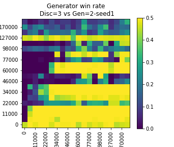
(f) D=3-BN vs G=2-BN

(g) D=1-BN vs G=3-BN

(h) D=2-BN vs G=3-BN

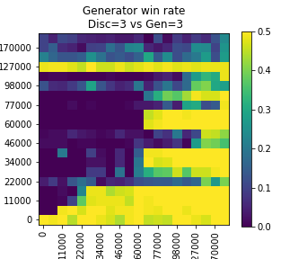
(i) D=3-BN vs G=3-BN

(j) D=1-BN vs G=4-cond-BN

(k) D=2-BN vs G=4-cond-BN

(l) D=3-BN vs G=4-cond-BN

Figure 11: Tournament heatmaps with batchnorm. This figure shows the same analysis as in Figure 6, but with batchnorm in the discriminators. Note the substantially darker heatmaps than those in Figure 6, indicating a lower overall generator win rate with the batchnorm discriminators than with the pixelnorm discriminators in these experiments. We believe this darker pattern is indicative of experiments without noise added to the discriminator input, rather than a property that separates batchnorm from pixelnorm.

(a) Real data samples
SR=1738
CS=8.09

(b) 1-BN
SR=1610
CS=6.27

(c) 4-cond-BN
SR=1594
CS=7.14

(d) 6-auto
SR=1568
CS=5.27

(e) 2-BN
SR=1511
CS=6.08

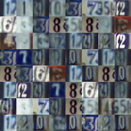
(f) 5-cond-BN
SR=1461
CS=7.85

(g) 3-BN
SR=1381
CS=5.50

(h) 1-bad-lr-BN
SR=1361
CS=4.67

Figure 12: Samples from fully-trained generative models with batchnorm.

Appendix D Appendix: Architectures

D.1 SVHN task training procedure, model architectures, and hyperparameters

Our SVHN GANs described in Section 4.2 are based off the DCGAN architecture, loss function, and hyperparameters from Gulrajani [2017], with small modifications. To all GANs, we add noise to the generated and real samples at training time (standard deviation of 0.2), and we substitute pixelnorm instead of batchnorm in the discriminator only (with an epsilon of $1e-5$) [Karras et al., 2017]. Experiment 1 is an otherwise-unmodified ordinary DCGAN. Experiment 3 is a Wasserstein GAN [Gulrajani, 2017]. Experiment 2 is a feature-matching GAN [Salimans et al., 2016]. Experiment 4-cond is a conditional GAN in which the label information is concatenated into the input to both generator and discriminator as an additional dimension. Experiment 5-cond is a conditional GAN in which the discriminator makes an 11-way judgment: 10 real classes or “fake”. All GAN models were trained for 200,000 steps with a learning rate of 0.0002 on both the generator and the discriminator. Experiment 6-auto is a PixelCNN++ [Salimans et al., 2017], trained using the code from https://github.com/openai/pixel-cnn, modified only to accept SVHN in place of CIFAR10.

We made no attempt to tune each model for its best possible performance, as it was advantageous for our purposes to allow sample quality to vary. As we emphasize in Section 4.2, our method is intended to compare the outcomes of individual experiments; we explicitly discourage an interpretation that we are comparing general algorithms.

Raw code for GAN architectures

All SVHN DCGAN variants used the architecture and hyperparameters described in the tensorflow code below. The different variants are defined by the flags in the code.

_HEIGHT, _WIDTH, _NUM_CHANNELS = [32, 32, 3]
WGAN_CRITIC_ITERS = 5


def _leaky_relu(x):
  return tf.maximum(0.2 * x, x)


def pixel_norm_nchw(x, eps=1e-8):
  return x * tf.rsqrt(tf.reduce_mean(tf.square(x), [1], keepdims=True) + eps)


def disc_inputs_with_labels(inputs, labels, scope, nplusone=False):
    height, width, _ = inputs.get_shape().as_list()[1:]
    # If fake_labels is not None, GAN is normal conditional.
    if nplusone:
      labels = None   # If nplusone, don’t ’show’ labels to D.
    if labels is not None:
      label_embedding = ops.linear.Linear(scope + ’.labels’, 10, height * width * 1, labels)
      label_embedding = _leaky_relu(label_embedding)
      label_embedding = tf.reshape(label_embedding, [-1, height, width, 1])
      inputs = tf.concat([inputs, label_embedding], axis=-1)
    return inputs


def ishaan_generator(z, fake_labels, is_training, stats_iter, scope, dim_z=128, add_to_collection=True):

    # If fake_labels is not None, GAN is conditional. Show fake_labels to G in that case.
    if fake_labels is not None:
      z = tf.concat([z, fake_labels], axis=-1)
      dim_z += fake_labels.get_shape().as_list()[-1]

    dim_g = 64
    output = ops.linear.Linear(scope + ’.Input’, dim_z, 4*4*4*dim_g, z)
    output = ops.batchnorm.Batchnorm(
        scope + ’.BN1’, [0], output, is_training=is_training, stats_iter=stats_iter)
    output = tf.nn.relu(output)
    output = tf.reshape(output, [-1, 4*dim_g, 4, 4])  # NCHW

    output = ops.deconv2d.Deconv2D(scope + ’.2’, 4*dim_g, 2*dim_g, 5, output)
    output = ops.batchnorm.Batchnorm(
        scope + ’.BN2’, [0,2,3], output, is_training=is_training, stats_iter=stats_iter)
    output = tf.nn.relu(output)

    output = ops.deconv2d.Deconv2D(scope + ’.3’, 2*dim_g, dim_g, 5, output)
    output = ops.batchnorm.Batchnorm(
        scope + ’.BN3’, [0,2,3], output, is_training=is_training, stats_iter=stats_iter)
    output = tf.nn.relu(output)

    output = ops.deconv2d.Deconv2D(scope + ’.5’, dim_g, 3, 5, output)

    output = tf.tanh(output)
    output = tf.reshape(output, [-1, _NUM_CHANNELS, _HEIGHT, _WIDTH])
    output = tf.transpose(output, [0, 2, 3, 1])  # move C back out to NHWC

    params = lib.params_with_name(scope, trainable_only=True)
    if add_to_collection:
      tf.add_to_collection(G_OUTPUT, output)
      tf.add_to_collection(G_PARAMS, params)
    return output, params


def pixelnorm_discriminator(inputs, labels, scope, add_to_collection=True, nplusone=False, eps=1e-8):

    inputs = disc_inputs_with_labels(inputs, labels, scope, nplusone)
    _, _, channels = inputs.get_shape().as_list()[1:]

    dim_d = 64
    output = tf.transpose(inputs, [0, 3, 1, 2])  # move C into NCHW
    output = ops.conv2d.Conv2D(scope + ’.1’, channels, dim_d, 5, output, stride=2)
    output = _leaky_relu(output)

    output = ops.conv2d.Conv2D(scope + ’.2’, dim_d, 2*dim_d, 5, output, stride=2)
    output = pixel_norm_nchw(output, eps)
    output = _leaky_relu(output)

    output = ops.conv2d.Conv2D(scope + ’.3’, 2*dim_d, 4*dim_d, 5, output,
                                      stride=2)
    output = pixel_norm_nchw(output, eps)
    output = _leaky_relu(output)

    output = tf.reshape(output, [-1, 4*4*4*dim_d])
    d_features = output  # for feature-matching

    if nplusone:
      output = ops.linear.Linear(scope + ’.Output’, 4*4*4*dim_d, 11, output)
    else:
      output = ops.linear.Linear(scope + ’.Output’, 4*4*4*dim_d, 1, output)
      output = tf.reshape(output, [-1])

    params = lib.params_with_name(scope, trainable_only=True)
    if add_to_collection:
      tf.add_to_collection(D_INPUT, inputs)
      tf.add_to_collection(D_OUTPUT, output)
      tf.add_to_collection(D_PARAMS, params)

    return output, params, d_features


def ns_discriminator_loss(d_on_data_logits, d_on_g_logits,
                          add_to_collection=True):
  loss = tf.reduce_mean(
    tf.nn.sigmoid_cross_entropy_with_logits(
      labels=tf.ones_like(d_on_data_logits), logits=d_on_data_logits) +
    tf.nn.sigmoid_cross_entropy_with_logits(
      labels=tf.zeros_like(d_on_g_logits), logits=d_on_g_logits))
  if add_to_collection:
    tf.add_to_collection(D_LOSS, loss)
  return loss


def ns_generator_loss(d_on_g_logits, add_to_collection=True):
  loss = tf.reduce_mean(tf.nn.sigmoid_cross_entropy_with_logits(
    labels=tf.ones_like(d_on_g_logits), logits=d_on_g_logits))
  if add_to_collection:
    tf.add_to_collection(G_LOSS, loss)
  return loss


def ns_train_op(cost, params, learning_rate, beta_1, collection=None):
  op = tf.train.AdamOptimizer(
    learning_rate, beta_1, 0.999).minimize(
    cost, var_list=params, colocate_gradients_with_ops=True)
  if collection:
    tf.add_to_collection(collection, op)
  return op


def nplusone_discriminator_loss(d_on_data_logits, d_on_g_logits,
                                real_labels, fake_labels,
                                add_to_collection=True):
  bsz = fake_labels.shape[0]

  augmented_real_labels = tf.zeros([bsz, 1])
  augmented_real_labels = tf.concat([real_labels, augmented_real_labels], -1)

  augmented_fake_labels = tf.ones([bsz, 1])
  augmented_fake_labels = tf.concat(
    [tf.zeros_like(fake_labels), augmented_fake_labels], -1)

  loss = tf.reduce_mean(
    tf.nn.softmax_cross_entropy_with_logits(
      labels=augmented_real_labels, logits=d_on_data_logits) +
    tf.nn.softmax_cross_entropy_with_logits(
      labels=augmented_fake_labels, logits=d_on_g_logits))
  if add_to_collection:
    tf.add_to_collection(D_LOSS, loss)
  return loss


def nplusone_generator_loss(d_on_g_logits, fake_labels, add_to_collection=True):
  bsz = fake_labels.shape[0]
  augmented_fake_labels = tf.zeros([bsz, 1])
  augmented_fake_labels = tf.concat([fake_labels, augmented_fake_labels], -1)

  loss = tf.reduce_mean(tf.nn.sigmoid_cross_entropy_with_logits(
    labels=augmented_fake_labels, logits=d_on_g_logits))
  if add_to_collection:
    tf.add_to_collection(G_LOSS, loss)
  return loss


def wgan_generator_loss(d_on_g_logits, add_to_collection=True):
  loss = -tf.reduce_mean(d_on_g_logits)
  if add_to_collection:
    tf.add_to_collection(G_LOSS, loss)
  return loss


def wgan_discriminator_loss(d_on_data_logits, d_on_g_logits,
                            add_to_collection=True):
  loss = tf.reduce_mean(d_on_g_logits) - tf.reduce_mean(d_on_data_logits)
  if add_to_collection:
    tf.add_to_collection(D_LOSS, loss)
  return loss


def wgan_train_op(cost, params, learning_rate, collection=None):
  op = tf.train.RMSPropOptimizer(learning_rate=learning_rate).minimize(
    cost, var_list=params)
  if collection:
    tf.add_to_collection(collection, op)
  return op


def wgan_clip_op(disc_params, add_to_collection=True):
  clip_ops = []
  for var in disc_params:
    clip_bounds = [-.01, .01]
    clip_ops.append(
      tf.assign(
        var,
        tf.clip_by_value(var, clip_bounds[0], clip_bounds[1])
        )
      )
  clip_disc_weights = tf.group(*clip_ops)
  if add_to_collection:
    tf.add_to_collection(CLIP_OP, clip_disc_weights)
  return clip_disc_weights


def feature_matching_generator_loss(d_g_features, d_data_features,
                                    add_to_collection=True):
  assert(len(d_g_features.shape) == 2)
  assert(len(d_data_features.shape) == 2)
  loss = tf.reduce_mean(tf.abs(
    tf.reduce_mean(d_g_features, axis=0) -
    tf.reduce_mean(d_data_features, axis=0)))
  if add_to_collection:
    tf.add_to_collection(G_LOSS, loss)
  return loss


def build_dcgan(dataset, batch_size=64, dim_z=128, learning_rate=2e-4,
                beta_1=0.5, graph=None, loss_variant=’dcgan’,
                eps=1e-8, ngrp=32, disc_noise=0.0,
                deterministic=False, tf_seed=TF_RNG_SEED,
                d_learning_rate=None, g_learning_rate=None):

  # Set default learning rates
  d_learning_rate = d_learning_rate or learning_rate
  g_learning_rate = g_learning_rate or learning_rate

  if graph is None:
    graph = tf.get_default_graph()
  if deterministic:
    tf.set_random_seed(tf_seed)

  with graph.as_default():
    # noise -> generated -> discriminator
    z = tf.random_normal([batch_size, dim_z])
    tf.add_to_collection(NOISE, z)

    real_data, real_labels = get_data_iterator(dataset, batch_size)
    if loss_variant in [’dcgan’, ’feature’, ’wgan’]:
      real_labels = None
      fake_labels = None
    elif loss_variant in [’conditional’, ’nplusone’]:
      real_labels = tf.one_hot(real_labels, 10)
      fake_labels = tf.random_uniform(shape=[batch_size,], minval=0,
                                          maxval=10, dtype=tf.int32)
      fake_labels = tf.one_hot(fake_labels, 10)

    generator_output, g_params = ishaan_generator(
      z, fake_labels, is_training=None, stats_iter=None,
      scope=G_SCOPE, dim_z=dim_z)

    noisy_gen = generator_output + tf.random_normal(
      [batch_size, _HEIGHT, _WIDTH, _NUM_CHANNELS],
      mean=0.0, stddev=disc_noise)
    noisy_real = real_data + tf.random_normal(
      [batch_size, _HEIGHT, _WIDTH, _NUM_CHANNELS],
      mean=0.0, stddev=disc_noise)

    nplusone = (loss_variant == ’nplusone’)

    d_on_g_logits, d_params, d_g_features = pixelnorm_discriminator(
      noisy_gen, fake_labels, scope=D_SCOPE, add_to_collection=True,
      nplusone=nplusone, eps=eps)
    d_on_data_logits, _, d_data_features = pixelnorm_discriminator(
      noisy_real, real_labels, scope=D_SCOPE, add_to_collection=False,
      nplusone=nplusone, eps=eps)

    # losses:
    if loss_variant == ’feature’:
      g_loss = feature_matching_generator_loss(d_g_features, d_data_features,
                                               add_to_collection=True)
      d_loss = ns_discriminator_loss(d_on_data_logits, d_on_g_logits,
                                    add_to_collection=True)
    elif loss_variant == ’dcgan’ or loss_variant == ’conditional’:
      g_loss = ns_generator_loss(d_on_g_logits, add_to_collection=True)
      d_loss = ns_discriminator_loss(d_on_data_logits, d_on_g_logits,
                                    add_to_collection=True)

    elif loss_variant == ’wgan’:
      g_loss = wgan_generator_loss(d_on_g_logits, add_to_collection=True)
      d_loss = wgan_discriminator_loss(d_on_data_logits, d_on_g_logits,
                                       add_to_collection=True)
    elif loss_variant == ’nplusone’:
      g_loss = nplusone_generator_loss(d_on_g_logits, fake_labels, add_to_collection=True)
      d_loss = nplusone_discriminator_loss(d_on_data_logits, d_on_g_logits,
                                           real_labels, fake_labels,
                                           add_to_collection=True)

    # opts:
    if loss_variant in [’dcgan’, ’feature’, ’conditional’, ’nplusone’]:
      ns_train_op(cost=g_loss, params=g_params, learning_rate=g_learning_rate,
                    beta_1=beta_1, collection=G_OPT)

      ns_train_op(cost=d_loss, params=d_params, learning_rate=d_learning_rate,
                    beta_1=beta_1, collection=D_OPT)

    elif loss_variant == ’wgan’:
      for (cost, params, collection) in [(g_loss, g_params, G_OPT),
                                         (d_loss, d_params, D_OPT)]:
        wgan_train_op(cost=cost, params=params, learning_rate=learning_rate,
                      collection=collection)

      wgan_clip_op(d_params)

D.2 "Gaussian Toy" task architecture and hyperparameters

For the “Gaussian Toy” task, we trained a small GAN (consisting of an MLP generator and an MLP discriminator with architectures described below) to estimate a 50-dimensional Gaussian. We additionally trained a separate Chekhov GAN. We show here the verbatim code from the Chekhov version. The vanilla toy GAN uses exactly the same architecture and training process, but without any past generators or discriminators.

Chekhov toy architecture

class ChekhovToy(object):
  """A toy Chekhov GAN which estimates a dim-dimensional Gaussian"""

  def __init__(self, data_dir=DATA_DIR, batch_size=BATCH_SIZE, dim=DIM,
               np_seed=NP_RNG_SEED, tf_seed=TF_RNG_SEED, deterministic=False,
               queue_size=1, queue_spacing=1000, reservoir=False):
    self.data_dir = data_dir
    self.batch_size = batch_size
    self.dim = dim
    self.queue_size = queue_size
    self.queue_spacing = queue_spacing

    self.reservoir = reservoir

    self.graph = tf.Graph()
    self.sess = tf.Session(graph=self.graph)
    self._loaded_from = None

    with self.graph.as_default():
      if deterministic:
        self.rng = np.random.RandomState(np_seed)
        tf.set_random_seed(tf_seed)
      else:
        self.rng = np.random.RandomState(None)

      self._build_model()
      self.sess.run(tf.global_variables_initializer())


  def _build_generator(self, name):
    generator = MLP(name=name,
      layers=[Linear(self.dim, init_scale=.05)],
        input_shape=[self.batch_size, self.dim])
    return generator


  def _build_discriminator(self, name):
    discriminator = MLP(name=name,
      layers=[
          Linear(1200),
          ReLU(),
          Linear(1200),
          ReLU(),
          Linear(100),
          ReLU(),
          Linear(1)
      ],
      input_shape=[self.batch_size, self.dim])
    return discriminator


  def _build_generator_loss(self, d_on_g_logits):
    return tf.reduce_mean(tf.nn.sigmoid_cross_entropy_with_logits(
        labels=tf.ones_like(d_on_g_logits), logits=d_on_g_logits))


  def _build_discriminator_loss(self, d_on_data_logits, d_on_g_logits):
    return tf.reduce_mean(
        tf.nn.sigmoid_cross_entropy_with_logits(
            labels=tf.ones_like(d_on_data_logits), logits=d_on_data_logits) +
        tf.nn.sigmoid_cross_entropy_with_logits(
            labels=tf.zeros_like(d_on_g_logits), logits=d_on_g_logits))


  def _build_model(self):

    ##### Data ######

    # Generate samples from dim-dimensional Gaussians
    self._true_mu = tf.Variable(self.rng.randn(self.dim).astype("float32"), trainable=False)
    self._true_cov = tf.Variable(self.rng.randn(self.dim, self.dim).astype("float32"), trainable=False)

    self._true_cov = tf.matmul(self._true_cov, self._true_cov, transpose_a=True)
    true_cov_chol = tf.Variable(tf.transpose(tf.cholesky(self._true_cov)), trainable=False)
    true_z = tf.random_normal([self.batch_size, self.dim])
    self._true_samples = tf.matmul(true_z, true_cov_chol) + self._true_mu


    ##### Generator ######

    # Creating the live/trainable generator.
    generator = self._build_generator(name="G_live")

    W, b = generator.get_params()
    assert len(W.get_shape()) == 2
    assert len(b.get_shape()) == 1

    # Compute moments
    self._gan_cov = tf.matmul(W, W, transpose_a=True)
    self._gan_mu = tf.identity(b)

    # Get MMD error signal
    self._err = {}
    self._err[’mmd’] = tf.maximum(
        tf.reduce_max(tf.abs(self._gan_cov - self._true_cov)),
        tf.reduce_max(tf.abs(self._gan_mu - self._true_mu)))
    self._err[’max_cov_diff’] = tf.reduce_max(tf.abs(self._gan_cov - self._true_cov))
    self._err[’max_mu_diff’] = tf.reduce_max(tf.abs(self._gan_mu - self._true_mu))
    self._err[’mean_cov_diff’] = tf.reduce_mean(tf.abs(self._gan_cov - self._true_cov))
    self._err[’mean_mu_diff’] = tf.reduce_mean(tf.abs(self._gan_mu - self._true_mu))
    self._err[’mean_sq_cov_diff’] = tf.reduce_mean(tf.square(self._gan_cov - self._true_cov))
    self._err[’mean_sq_mu_diff’] = tf.reduce_mean(tf.square(self._gan_mu - self._true_mu))

    z = tf.random_normal([self.batch_size, self.dim])
    self._gan_samples = generator.fprop(z)


    ##### Discriminator #####

    # Creating the live/trainable discriminator
    discriminator = self._build_discriminator(name="D_live")
    d_on_data_logits = tf.squeeze(discriminator.fprop(self._true_samples))
    d_on_g_logits = tf.squeeze(discriminator.fprop(self._gan_samples))

    # Discriminate placeholder
    self._discriminate_input = tf.placeholder(tf.float32, shape=(self.batch_size, self.dim))
    self._discriminate_output = discriminator.fprop(self._discriminate_input)


    ##### Past G/D queue #####

    # Discriminator queue: old D’s classify the current G’s samples
    self._curr_g_old_d_losses = []
    self._d_queue_assign_ops = []

    for i in range(self.queue_size):
      past_d_i = self._build_discriminator(name="D_queue_{}".format(i))

      past_d_on_curr_g_logits = tf.squeeze(past_d_i.fprop(self._gan_samples))
      self._curr_g_old_d_losses.append(self._build_generator_loss(
        d_on_g_logits=past_d_on_curr_g_logits))

      self._d_queue_assign_ops.append(past_d_i.assign_params(
        discriminator.get_params(collapse=False)))

    # Generator queue: the current D classifies old G’s samples
    self._curr_d_old_g_losses = []
    self._g_queue_assign_ops = []

    for i in range(self.queue_size):
      past_g_i = self._build_generator(name="G_queue_{}".format(i))
      z_i = tf.random_normal([self.batch_size, self.dim])
      past_samples_i = past_g_i.fprop(z_i)
      d_on_past_g_logits = tf.squeeze(discriminator.fprop(past_samples_i))
      self._curr_d_old_g_losses.append(self._build_discriminator_loss(
          d_on_g_logits=d_on_past_g_logits,
          d_on_data_logits=d_on_data_logits))

      self._g_queue_assign_ops.append(past_g_i.assign_params(
        generator.get_params(collapse=False)))


    ##### Loss & optimizers ######

    # Compute d_loss and g_loss
    self._d_curr_loss = self._build_discriminator_loss(
        d_on_data_logits=d_on_data_logits,
        d_on_g_logits=d_on_g_logits)
    self._g_curr_loss = self._build_generator_loss(d_on_g_logits)

    # Build a whole list of optimizers, depending on how full the queue is...
    self._d_losses = []
    self._d_opts = []
    self._g_losses = []
    self._g_opts = []
    for i in range(self.queue_size + 1):
      _d_loss_i = tf.reduce_mean(self._curr_d_old_g_losses[:i] + [self._d_curr_loss])
      _g_loss_i = tf.reduce_mean(self._curr_g_old_d_losses[:i] + [self._g_curr_loss])

      self._d_losses.append(_d_loss_i)
      self._g_losses.append(_g_loss_i)

      # NB: this does NOT include the L2 regularizer from Chekhov GAN
      d_optimizer = tf.train.AdamOptimizer(learning_rate=1e-3)
      g_optimizer = tf.train.AdamOptimizer(learning_rate=1e-3)

      _d_opt_i = d_optimizer.minimize(_d_loss_i, var_list=discriminator.get_params())
      _g_opt_i = g_optimizer.minimize(_g_loss_i, var_list=generator.get_params())

      self._d_opts.append(_d_opt_i)
      self._g_opts.append(_g_opt_i)


    ##### Saver ######
    self._saver = tf.train.Saver(max_to_keep=None)


  def load(self, modelID):
    if self._loaded_from != modelID:
      with self.sess.as_default():
        with self.graph.as_default():
          self._saver.restore(
              self.sess, os.path.join(logdir(modelID.experiment),
                                      modelID.experiment + "-{}".format(modelID.iteration)))
          self._loaded_from = modelID

  def save(self, experiment_name, global_step):
    assert(experiment_name)
    self._saver.save(
      self.sess,
      os.path.join(logdir(experiment_name), experiment_name),
      global_step=global_step,
      write_meta_graph=(global_step == 0))


  def _should_evict_now(self, i):
    if self.queue_size == 0 or i == 0:
      return False

    else:
      if self.reservoir:
        return (i < self.queue_size or
                np.random.random() > (self.queue_size / i))
      else:
        return i % self.queue_spacing


  def train(self, steps=16000, experiment_name=None, save=False):
    with self.sess.as_default():
      with self.graph.as_default():
        row_format_s = "{:^10} | {:^16} | {:^16} | {:^16} | {:^16} | {:^16}"
        row_format = "{:^10} | {:^16.1e} | {:^16.1e}| {:^16.1e}| {:^16.1e} | {:^16.4f}"
        print(row_format_s.format("Iteration", "D total loss", "D curr loss",
                                  "G total loss", "G curr loss", "MMD"))
        print("=" * 98)

        queue_idx = 0
        queue_full = False
        for i in xrange(steps + 1):

          # Update queues if it’s time to do so
          if self._should_evict_now(i):
            self.sess.run(self._d_queue_assign_ops[queue_idx])
            self.sess.run(self._g_queue_assign_ops[queue_idx])

            if not queue_full and (queue_idx + 1) == self.queue_size:
              queue_full = True

            if queue_full and self.reservoir:
              queue_idx = np.random.randint(self.queue_size)  # if reservoir sampling into a full queue, evict randomly
            else:
              queue_idx = (queue_idx + 1) % self.queue_size  # otherwise, march through in an orderly fashion

          # Choose the loss function - if the queue isn’t full, don’t backprop through the unused slots
          if not queue_full:
            loss_idx = queue_idx
          else:
            loss_idx = self.queue_size

          # Print out
          if i % 1000 == 0:
            # Eval
            d_loss, d_curr_loss, g_loss, g_curr_loss, err = self.sess.run([
                self._d_losses[loss_idx],
                self._d_curr_loss,
                self._g_losses[loss_idx],
                self._g_curr_loss,
                self._err
            ])
            print(row_format.format(i, d_loss, d_curr_loss, g_loss, g_curr_loss, err))

            # Save
            if save:
              self.save(experiment_name, i)


          # Train
          self.sess.run([self._d_opts[loss_idx], self._g_opts[loss_idx]])

References

- Arora et al. (2018) Sanjeev Arora, Andrej Risteski, and Yi Zhang. Do GANs learn the distribution? some theory and empirics. In International Conference on Learning Representations, 2018. URL https://openreview.net/forum?id=BJehNfW0-.
- Borji (2018) A. Borji. Pros and cons of gan evaluation measure. arXiv:1802.03446, Feb 2018. URL https://arxiv.org/pdf/1802.03446.
- Breuleux et al. (2010) Olivier Breuleux, Yoshua Bengio, and Pascal Vincent. Unlearning for better mixing. Technical Report 1349, Université de Montréal/DIRO, 2010.
- Denton et al. (2015) Emily Denton, Soumith Chintala, Arthur Szlam, and Rob Fergus. Deep generative image models using a Laplacian pyramid of adversarial networks. NIPS, 2015.
- Durugkar et al. (2017) Ishan Durugkar, Ian Gemp, and Sridhar Mahadevan. Generative multi-adversarial networks. ICLR, 2017. URL https://arxiv.org/pdf/1611.01673.pdf. arXiv:1611.01673.
- Elo (1978) A. Elo. The rating of chessplayers, past and present. Arco Pub., New York, 1978. ISBN 0668047216 9780668047210.
- Glickman (1995) M. Glickman. A comprehensive guide to chess ratings. 1995. URL http://www.glicko.net/research/acjpaper.pdf.
- Glickman (2013) M. Glickman. Example of the glicko-2 system. Nov 2013. URL http://www.glicko.net/glicko/glicko2.pdf.
- Goodfellow (2014) Ian J. Goodfellow. On distinguishability criteria for estimating generative models. In International Conference on Learning Representations, Workshops Track, 2014.
- Goodfellow et al. (2014) Ian J. Goodfellow, Jean Pouget-Abadie, Mehdi Mirza, Bing Xu, David Warde-Farley, Sherjil Ozair, Aaron Courville, and Yoshua Bengio. Generative adversarial networks. In NIPS’2014, 2014.
- Grnarova et al. (2017) P. Grnarova, K. Levy, A. Lucchi, T. Hofmann, and A. Krause. An online learning approach to generative adversarial networks. arXiv:1706.03269, Jun 2017. URL https://arxiv.org/abs/1706.03269.
- Gulrajani (2017) I. Gulrajani. Improved training of wasserstein gans. https://github.com/igul222/improved_wgan_training, 2017. fa66c574a54c4916d27c55441d33753dcc78f6bc.
- Gutmann and Hyvarinen (2010) M. Gutmann and A. Hyvarinen. Noise-contrastive estimation: A new estimation principle for unnormalized statistical models. In aistats10, 2010.
- Ha and Eck (2017) D. Ha and D. Eck. A neural representation of sketch drawings. arXiv:1704.03477, Apr 2017. URL https://arxiv.org/abs/1704.03477.
- Herbrich et al. (2007) Ralf Herbrich, Tom Minka, and Thore Graepel. Trueskill: a bayesian skill rating system. In Advances in neural information processing systems, pages 569–576, 2007.
- Heusel et al. (2017) M. Heusel, H. Ramsauer, T. Unterthiner, B. Nessler, and S. Hochreiter. Gans trained by a two time-scale update rule converge to a local nash equilibrium. In Advances in Neural Information Processing Systems 30. 2017. URL http://papers.nips.cc/paper/7240-gans-trained-by-a-two-time-scale-update-rule-converge-to-a-local-nash-equilibrium.pdf.
- Im et al. (2016) Daniel Jiwoong Im, Chris Dongjoo Kim, Hui Jiang, and Roland Memisevic. Generating images with recurrent adversarial networks. arXiv preprint arXiv:1602.05110, 2016.
- Karras et al. (2017) Tero Karras, Timo Aila, Samuli Laine, and Jaakko Lehtinen. Progressive growing of gans for improved quality, stability, and variation. CoRR, abs/1710.10196, 2017. URL http://arxiv.org/abs/1710.10196.
- Netzer et al. (2011) Y. Netzer, T. Wang, A. Coates, A. Bissacco, B. Wu, and A. Ng. Reading digits in natural images with unsupervised feature learning. In NIPS Workshop on Deep Learning and Unsupervised Feature Learning. 2011. URL http://ufldl.stanford.edu/housenumbers/.
- OpenAI (2017) OpenAI. More on dota 2. https://blog.openai.com/more-on-dota-2/, Aug 2017.
- Radford et al. (2015) A. Radford, L. Metz, and S. Chintala. Unsupervised representation learning with deep convolutional generative adversarial networks. arXiv:1511.06434, Nov 2015. URL https://arxiv.org/abs/1511.06434.
- Salimans et al. (2016) T. Salimans, I. Goodfellow, W. Zaremba, V. Cheung, A. Radford, and X. Chen. Improved techniques for training gans. In Advances in Neural Information Processing Systems 29. 2016. URL http://papers.nips.cc/paper/6125-improved-techniques-for-training-gans.pdf.
- Salimans et al. (2017) T. Salimans, A. Karpathy, X. Chen, and D. Kingma. Pixelcnn++: Improving the pixelcnn with discretized logistic mixture likelihood and other modifications. arXiv:1701.05517, Jan 2017. URL https://arxiv.org/abs/1701.05517.
- Santurkar et al. (2018) Shibani Santurkar, Ludwig Schmidt, and Aleksander Madry. A classification-based perspective on GAN distributions, 2018. URL https://openreview.net/forum?id=S1FQEfZA-.
- Silberman et al. (2015) S. Silberman, K. Milland, R. LaPlante, J. Ross, and L. Irani. Stop citing ross et al. 2010, “who are the crowdworkers”? https://medium.com/@silberman/stop-citing-ross-et-al-2010-who-are-the-crowdworkers-b3b9b1e8d300, Mar 2015.
- Silver et al. (2016) David Silver, Aja Huang, Chris J Maddison, Arthur Guez, Laurent Sifre, George Van Den Driessche, Julian Schrittwieser, Ioannis Antonoglou, Veda Panneershelvam, Marc Lanctot, et al. Mastering the game of go with deep neural networks and tree search. nature, 529(7587):484, 2016.
- Szegedy et al. (2015) C. Szegedy, V. Vanhoucke, S. Ioffe, J. Shlens, and Z. Wojna. Rethinking the Inception Architecture for Computer Vision. ArXiv e-prints, December 2015.
- Theis et al. (2016) L. Theis, A. van den Oord, and M. Bethge. A note on the evaluation of generative models. arXiv:1511.01844, 2016. URL http://arxiv.org/abs/1511.01844.