Two Local Models for Neural Constituent Parsing

Non-local features have been exploited by syntactic parsers for capturing dependencies between sub output structures. Such features have been a key to the success of state-of-the-art statistical parsers. With the rise of deep learning, however, it has been shown that local output decisions can give highly competitive accuracies, thanks to the power of dense neural input representations that embody global syntactic information. We investigate two conceptually simple local neural models for constituent parsing, which make local decisions to constituent spans and CFG rules, respectively. Consistent with previous findings along the line, our best model gives highly competitive results, achieving the labeled bracketing F1 scores of 92.4% on PTB and 87.3% on CTB 5.1.

1 Introduction

Non-local features have been shown crucial for statistical parsing [Huang (2008a, Zhang and Nivre (2011]. For dependency parsing, High-order dynamic programs [Koo and Collins (2010], integer linear programming [Martins et al. (2010] and dual decomposition [Koo et al. (2010] techniques have been exploited by graph-based parser to integrate non-local features. Transition-based parsers [Nivre (2003, Nivre (2008, Zhang and Nivre (2011, Bohnet (2010, Huang et al. (2012] are also known for leveraging non-local features for achieving high accuracies. For most state-of-the-art statistical parsers, a global training objective over the entire parse tree has been defined to avoid label bias [Lafferty et al. (2001].

For neural parsing, on the other hand, local models have been shown to give highly competitive accuracies [Cross and Huang (2016b, Stern et al. (2017] as compared to those that employ long-range features [Watanabe and Sumita (2015, Zhou et al. (2015, Andor et al. (2016, Durrett and Klein (2015]. Highly local features have been used in recent state-of-the-art models [Stern et al. (2017, Dozat and Manning (2016, Shi et al. (2017]. In particular, ?) show that a locally trained arc-factored model can give the best reported accuracies on dependency parsing. The surprising result has been largely attributed to the representation power of long short-term memory (LSTM) encoders [Kiperwasser and Goldberg (2016b].

An interesting research question is to what extent the encoding power can be leveraged for constituent parsing. We investigate the problem by building a chart-based model that is local to unlabeled constituent spans [Abney (1991] and CFG-rules, which have been explored by early PCFG models [Collins (2003, Klein and Manning (2003]. In particular, our models first predict unlabeled CFG trees leveraging bi-affine modelling [Dozat and Manning (2016]. Then, constituent labels are assigned on unlabeled trees by using a tree-LSTM to encode the syntactic structure, and a LSTM decoder for yielding label sequences on each node, which can include unary rules.

Experiments show that our conceptually simple models give highly competitive performances compared with the state-of-the-art. Our best models give labeled bracketing F1 scores of 92.4% on PTB and 87.3% on CTB 5.1 test sets, without reranking, ensembling and external parses. We release our code at https://github.com/zeeeyang/two-local-neural-conparsers.

2 Model

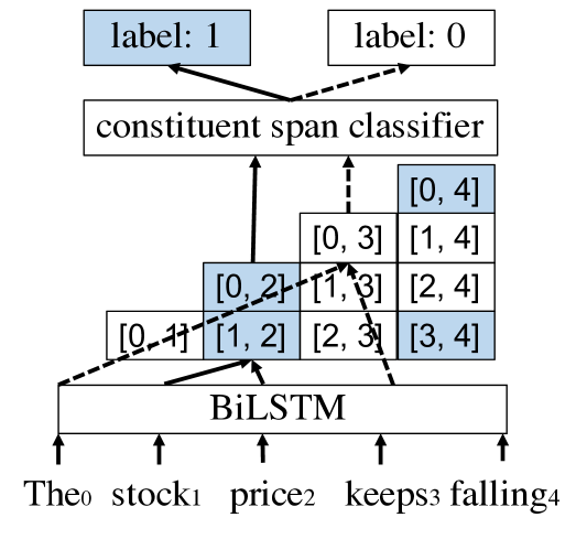
(a) BiLSTM based constituent span classifier.

(b) unlabeled binarized parse tree.

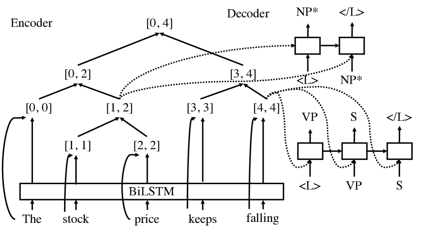
(c) Label generator for two example spans. NP* is an intermediate constituent label.

(d) Final example parse tree.

Figure 1: An example workflow of our parsers for the sentence “The stock price keeps falling”. We annotate every non-terminal span with its covered span range. Figure 1(a) shows constituent span classifiers making 0/1 decisions for all possible spans. Based on the local classification probabilities, we obtain an unlabeled binarized parse tree (Figure 1(b)) using binary CKY parsing algorithms. We then hierarchically generate labels for each span (Figure 1(c)) using encoder-decoder models. Figure 1(d) shows the final output parse tree after debinarization.

Our models consist of an unlabeled binarized tree parser and a label generator. Figure 1 shows a running example of our parsing model. The unlabeled parser (Figure 1(a), 1(b)) learns an unlabeled parse tree using simple BiLSTM encoders [Hochreiter and Schmidhuber (1997]. The label generator (Figure 1(c), 1(d)) predicts constituent labels for each span in the unlabeled tree using tree-LSTM models.

In particular, we design two different classification models for unlabeled parsing: the span model (Section 2.1) and the rule model (Section 2.2). The span model identifies the probability of an arbitrary span being a constituent span. For example, the span $[1,2]$ in Figure 1(a) belongs to the correct parse tree (Figure 1(d)). Ideally, our model assigns a high probability to this span. In contrast, the span $[0,3]$ is not a valid constituent span and our model labels it with 0. Different from the span model, the rule model considers the probability $P([i,j]\rightarrow[i,k][k+1,j]|S)$ for the production rule that the span $[i,j]$ is composed by two children spans $[i,k]$ and $[k+1,j]$, where $i\leq k<j$. For example, in Figure 1(a), the rule model assigns high probability to the rule $[0,2]\rightarrow[0,0][1,2]$ instead of the rule $[0,2]\rightarrow[0,1][2,2]$. Given the local probabilities, we use CKY algorithm to find the unlabeled binarized parses.

The label generator encodes a binarized unlabeled tree and to predict constituent labels for every span. The encoder is a binary tree-LSTM [Tai et al. (2015, Zhu et al. (2015], which recursively composes the representation vectors for tree nodes bottom-up. Based on the representation vector of a constituent span, a LSTM decoder [Cho et al. (2014, Sutskever et al. (2014] generates chains of constituent labels, which can represent unary rules. For example, the decoder outputs “VP $\rightarrow$S$\rightarrow$ $<$/L$>$” for the span [4, 4] and “NP$\rightarrow$ $<$/L$>$” for the span [0,2] in Figure 1(c) where $<$/L$>$ is a stopping symbol.

2.1 Span Model

Given an unlabeled binarized tree $T_{ub}$ for the sentence $S$, $S=w_{0},w_{1}\dots w_{n-1}$, the span model trains a neural network model $P(Y_{[i,j]}|S,\Theta)$ to distinguish constituent spans from non-constituent spans, where $0\leq i\leq n-2$, $1\leq j<n$, $i<j$. $Y_{[i,j]}=1$ indicates the span [i, j] is a constituent span ($[i,j]\in T_{ub}$), and $Y_{[i,j]}=0$ for otherwise, $\Theta$ are model parameters. We do not model spans with length 1 since the span $[i,i]$ always belongs to $T_{ub}$.

Network Structure. Figure 2(a) shows the neural network structures for the binary classification model. In the bottom, a bidirectional LSTM layer encodes the input sentence to extract non-local features. In particular, we append a starting symbol $<$s$>$ and an ending symbol $<$/s$>$ to the left-to-right LSTM and the right-to-left LSTM, respectively. We denote the output hidden vectors of the left-to-right LSTM and the right-to-left LSTM for $w_{0},w_{1},\dots,w_{n-1}$ is $\mathbf{f}_{1},\mathbf{f}_{2},\dots,\mathbf{f}_{n}$ and $\mathbf{r}_{0},\mathbf{r}_{1},\dots,\mathbf{r}_{n-1}$, respectively. We obtain the representation vector $\mathbf{v}[i,j]$ of the span $[i,j]$ by simply concatenating the bidirectional output vectors at the input word $i$ and the input word $j$,

$$\mathbf{v}[i,j]=[\mathbf{f}_{i+1};\mathbf{r}_{i};\mathbf{f}_{j+1};\mathbf{r}_{j}].$$ (1)

$\mathbf{v}[i,j]$ is then passed through a nonlinear transformation layer and the probability distribution $P(Y_{[i,j]}|S,\Theta)$ is given by

$$\mathbf{o}[i,j]=\tanh(\mathbf{W}_{o}\mathbf{v}[i,j]+\mathbf{b}_{o}),\ \ \mathbf{u}[i,j]=\mathbf{W}_{u}\mathbf{o}[i,j]+\mathbf{b}_{u},\ \ P(Y_{[i,j]}|S,\Theta)=\text{softmax}(\mathbf{u}[i,j]),$$ (2)

where $\mathbf{W}_{o},\mathbf{b}_{o},\mathbf{W}_{u}$ and $\mathbf{b}_{u}$ are model parameters.

Input Representation. Words and part-of-speech (POS) tags are integrated to obtain the input representation vectors. Given a word $w$, its corresponding characters $c_{0},\dots,c_{|w|-1}$ and POS tag $t$, first, we obtain the word embedding $\mathbf{E}_{word}^{w}$, character embeddings $\mathbf{E}_{char}^{c_{0}},\dots,\mathbf{E}_{char}^{c_{|w|-1}}$, and POS tag embedding $\mathbf{E}_{pos}^{t}$ using lookup operations. Then a bidirectional LSTM is used to extract character-level features. Suppose that the last output vectors of the left-to-right and right-to-left LSTMs are $\mathbf{h}_{char}^{f}$ and $\mathbf{h}_{char}^{r}$, respectively. The final input vector $\mathbf{x}_{input}$ is given by

$$\mathbf{x}_{char}=\tanh(\mathbf{W}_{char}^{l}\mathbf{h}_{char}^{l}+\mathbf{W}_{char}^{r}\mathbf{h}_{char}^{r}+\mathbf{b}_{char}),\ \ \mathbf{x}_{input}=[\mathbf{E}_{word}^{w}+\mathbf{x}_{char};\mathbf{E}_{pos}^{t}],$$ (3)

where $\mathbf{W}_{char}^{l}$, $\mathbf{W}_{char}^{r}$ and $\mathbf{b}_{char}$ are model parameters.

Training objective. The training objective is to maximize the probabilities of $P(Y_{[i,j]}=1|S,\Theta)$ for spans $[i,j]\in T_{ub}$ and minimize the probabilities of $P(Y_{[i,j]}=1|S,\Theta)$ for spans $[i,j]\notin T_{ub}$ at the same time. Formally, the training loss for binary span classification ${\mathcal{L}}_{\text{binary}}$ is given by

$$\begin{split}{\mathcal{L}}_{\text{binary}}=-\sum_{[i,j]\in T_{ub}}&{\log P(Y_{[i,j]}=1|S,\Theta)}-\sum_{[i,j]\notin T_{ub}}{\log P(Y_{[i,j]}=0|S,\Theta)},\\ &(0\leq i\leq n-2,1\leq j<n,i<j)\end{split}$$ (4)

For a sentence with length $n$, there are $\frac{n(n-1)}{2}$ terms in total in Eq 4.

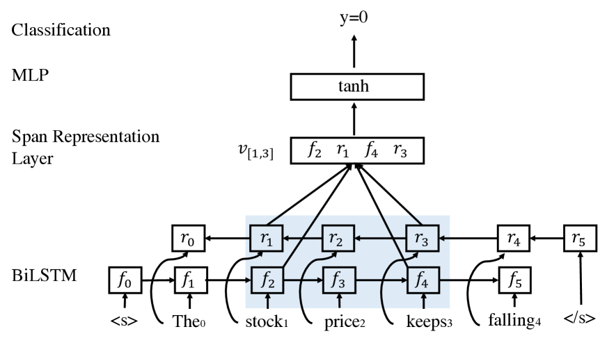
(a) Span model.

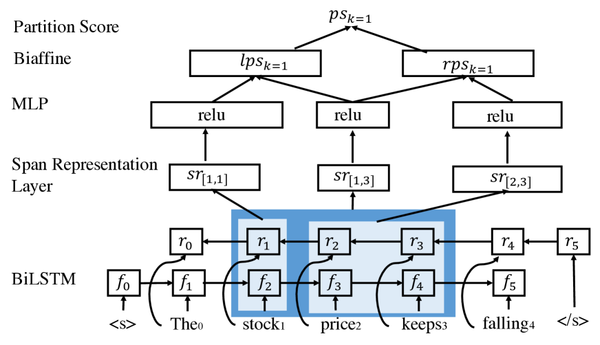
(b) Rule model.

Figure 2: Neural network structures for span and rule models using BiLSTM encoders.

Neural CKY algorithm. The unlabeled production probability for the rule $r:[i,j]\rightarrow[i,k][k+1,j]$ given by the binary classification model is,

$$P(r|S,\Theta)=P(Y_{[i,k]}=1|S,\Theta)P(Y_{[k+1,j]}=1|S,\Theta).$$

During decoding, we find the optimal parse tree $T_{ub}^{*}$ using the CKY algorithm. Note that our CKY algorithm is different from the standard CKY algorithm mainly in that there is no explicit phrase rule probabilities being involved. Hence our model can be regarded as a zero-order constituent tree model, which is the most local. All structural relations in a constituent tree must be implicitly captured by the BiLSTM encoder over the sentence alone.

Multi-class Span Classification Model. The previous model preforms binary classifications to identify constituent spans. In this way, the classification model only captures the existence of constituent labels but does not leverage constituent label type information. In order to incorporate the syntactic label information into the span model, we use a multi-class classification model $P(Y_{[i,j]}=c|S,\Theta)$ to describe the probability that $c$ is a constituent label for span $[i,j]$. The network structure is the same as the binary span classification model except the last layer. For the last layer, given $\mathbf{o}_{[i,j]}$ in Eq 2, $P(Y_{[i,j]}=c|S,\Theta)$ is calculated by,

$$\mathbf{m}[i,j]=\mathbf{W}_{m}\mathbf{o}[i,j]+\mathbf{b}_{m},\ P(Y_{[i,j]}=c|S,\Theta)=\text{softmax}(\mathbf{m}[i,j])_{[c]}.$$ (5)

Here $\mathbf{W}_{m},\mathbf{b}_{m},\mathbf{W}_{m}$ and $\mathbf{b}_{m}$ are model parameters. The subscript $[c]$ is to pick the probability for the label $c$. The training loss is,

$$\begin{split}\mathcal{L}_{\text{multi}}=-\sum_{[i,j]\in T_{ub}}\sum_{c\in\textsc{Gen}[i,j],c\neq\text{\textless}/L\text{\textgreater}}&{\log P(Y_{[i,j]}=c|S,\Theta)}-\sum_{[i,j]\notin T_{ub}}{\log P(Y_{[i,j]}=\text{\textless}/L\text{\textgreater}|S,\Theta)},\\ &(0\leq i\leq n-2,1\leq j<n,i<j)\\ \end{split}$$ (6)

Note that there is an additional sum inside the first term in Eq 6, which is different from the first term in Eq 4. $\textsc{Gen}[i,j]$ denotes the label set of span $[i,j]$. This is to say that we treat all constituent labels equally of a unary chain. For example, suppose there is a unary chain S$\rightarrow$VP in span [4,4]. For this span, we hypothesize that both labels are plausible answers and pay equal attentions to VP and S during training. For the second term in Eq 6, we maximize the probability of the ending label for non-constituent spans.

For decoding, we transform the multi-class probability distribution into a binary probability distribution by using,

$$P(Y_{[i,j]}=1|S,\Theta)=\sum_{c,c\neq\text{\textless}/L\text{\textgreater}}{P(Y_{[i,j]}=c|S,\Theta)},\ \ P(Y_{[i,j]}=0|S,\Theta)=P(Y_{[i,j]}=\text{\textless}/L\text{\textgreater}|S,\Theta)$$

In this way, the probability of a span being a constituent span takes all possible syntactic labels into considerations.

2.2 Rule Model

The rule model directly calculates the probabilities of all possible splitting points $k$ ($i\leq k<j)$ for the span $[i,j]$. Suppose the partition score of splitting point $k$ is $ps_{k}$. The unlabeled production probability for the rule $r:[i,j]\rightarrow[i,k][k+1,j]$ is given by a softmax distribution,

$$P([i,j]\rightarrow[i,k][k+1,j]|S,\Theta)=\frac{\exp(ps_{k})}{\sum_{k^{\prime}=i}^{j-1}{\exp(ps_{k^{\prime}})}}.$$

The training objective is to minimize the log probability loss of all unlabeled production rules.

$${\mathcal{L}}_{\text{rule}}=-\sum_{r\in{T_{ub}}}\log P(r:[i,j]\rightarrow[i,k][k+1,j]|S,\Theta)$$

The decoding algorithm is the standard CKY algorithm, which we omit here. The rule model can be regarded as a first-order constituent model, with the probability of each phrase rule being modeled. However, unlike structured learning algorithms [Finkel et al. (2008, Carreras et al. (2008], which use a global score for each tree, our model learns each production rule probability individually. Such local learning has traditionally been found subjective to label bias [Lafferty et al. (2001]. Our model relies on input representations solely for resolving this issue.

Span Representation. Figure 2(b) shows one possible network architecture for the rule model by taking the partition point $k=1$ for the span $[1,3]$ as an example. The BiLSTM encoder layer in the bottom is the same as that of the previous span classification model. We obtain the span representation vectors using difference vectors [Wang and Chang (2016, Cross and Huang (2016b]. Formally, the span representation vector $\mathbf{sr}[i,j]$ is given by,

$$\begin{split}\mathbf{s}[i,j]&=[\mathbf{f}_{j+1}-\mathbf{f}_{i};\mathbf{r}_{i}-\mathbf{r}_{j+1}],\\ \mathbf{sr}[i,j]&=[\mathbf{s}[0,i-1];\mathbf{s}[i,j];\mathbf{s}[j+1,n-1]].\end{split}$$ (7)

We first combine the difference vectors $(\mathbf{f}_{j+1}-\mathbf{f}_{i})$ and $(\mathbf{r}_{i}-\mathbf{r}_{j+1})$ to obtain a simple span representation vector $\mathbf{s}[i,j]$. In order to take more contextual information such as $\mathbf{f}_{p}$ where $p>j+1$ and $\mathbf{r}_{q}$ where $q<i$, we concatenate $\mathbf{s}[0,i-1]$, $\mathbf{s}[i,j]$, and $\mathbf{s}[j+1,n-1]$ to produce the final span representation vector $\mathbf{sr}[i,j]$. We then transform $\mathbf{sr}[i,j]$ to an output vector $\mathbf{r}[i,j]$ using an activation function $\phi$,

$$\mathbf{r}[i,j]=\phi(\mathbf{W}_{r}^{M}\mathbf{sr}[i,j]+\mathbf{b}_{r}^{M}),$$ (8)

where $\mathbf{W}_{r}^{M}$ and $\mathbf{b}_{r}^{M}$ and model parameters, and $M$ is a parameter set index. We use separate parameters for the nonlinear transforming layer. $M\in\{P,L,R\}$ are for the parent span $[i,j]$, the left child span $[i,k]$ and the right child span $[k+1,j]$, respectively.

After obtaining the span representation vectors, we use these vectors to calculate the partition score $ps_{k}$. In particular, we investigate two scoring methods.

Linear Model. In the linear model, the partition score is calculated by a linear affine transformation. For the splitting point $k$,

$$ps_{k}=\mathbf{w}_{ll,k}^{T}\mathbf{r}[i,k]+\mathbf{w}_{lr,k}^{T}\mathbf{r}[k+1,j]+{b}_{ll,k}$$

where $\mathbf{w}_{ll,k}^{T}$ and $\mathbf{w}_{ll,k}^{T}$ are two vectors, and ${b}_{ll,k}$ is a size 1 parameter.

Biaffine model. Since the possible splitting points for spans are varied with the length of span, we also try a biaffine scoring model (as shown in Figure 2(b)), which is good at handling variable-sized classification problems [Dozat and Manning (2016, Ma and Hovy (2017]. The biaffine model produces the score ${lps}_{k}$ between the parent span $[i,j]$ and the left child span $[i,k]$ using a biaffine scorer

$${lps}_{k}=(\mathbf{r}[i,j]\oplus 1)^{T}\mathbf{W}_{pl}(\mathbf{r}[i,k]\oplus 1)$$ (9)

where $\mathbf{W}_{pl}$ is model parameters and $\oplus$ denotes vector concatenation. Similarly, we calculate the score ${rps}_{k}$ between the parent span $[i,j]$ and the right child span $[k+1,j]$ using $\mathbf{W}_{pr}$ and $\mathbf{b}_{pr}$ as parameters. The overall partition score ${ps}_{k}$ is therefore given by

$${ps}_{k}={lps}_{k}+{rps}_{k}.$$

2.3 Label Generator

Lexicalized Tree-LSTM Encoder. Shown in Figure 1(c), we use lexicalized tree LSTM [Teng and Zhang (2016] for encoding, which shows good representation abilities for unlabeled trees. The encoder first propagates lexical information from two children spans to their parent using a lexical gate, then it produces the representation vectors of the parent span by composing the vectors of children spans using a binarized tree-LSTM [Tai et al. (2015, Zhu et al. (2015]. Formally, the lexical vector $\mathbf{tx}[i,j]$ for the span $[i,j]$ with the partition point at $k$ is defined by:

$$\begin{split}\mathbf{i}_{[i,j]}^{lex}&=\sigma(\mathbf{W}_{l}^{lex}\mathbf{tx}{[i,k]}+\mathbf{W}_{r}^{lex}\mathbf{tx}{[k+1,j]}+\mathbf{W}_{lh}^{lex}\mathbf{h}_{[i,k]}+\mathbf{W}_{rh}^{lex}\mathbf{h}_{[k+1,j]}+\mathbf{b}_{lex})\\ \mathbf{tx}[i,j]&=\mathbf{i}_{[i,j]}^{lex}\odot\mathbf{tx}{[i,k]}+(\mathbf{1.0}-\mathbf{i}_{[i,j]}^{lex})\odot\mathbf{tx}{[k+1,j]},\\ \end{split}$$

where $\mathbf{W}_{l}^{lex}$, $\mathbf{W}_{r}^{lex}$ and $\mathbf{b}_{lex}$ are model parameters, $\odot$ is element-wise multiplication and $\sigma$ is the logistic function. The lexical vector $\mathbf{tx}[i,i]$ for the leaf node $i$ is the concatenate of the output vectors of the BiLSTM encoder and the input representation $\mathbf{x}_{\textbf{input}}[i]$ (Eq 3), as shown in Figure 1(c).

The output state vector $\mathbf{h}[i,j]$ of the span $[i,j]$ given by a binary tree LSTM encoder is,

$$\begin{split}&\mathbf{i}_{p}=\sigma(\mathbf{W}_{1}\mathbf{tx}_{p}+\mathbf{W}_{2}\mathbf{h}_{l}+\mathbf{W}_{3}\mathbf{c}_{l}+\mathbf{W}_{4}\mathbf{h}_{r}+\mathbf{W}_{5}\mathbf{c}_{r}+\mathbf{b}_{1}),\\ &\mathbf{f}_{p}^{l}=\sigma(\mathbf{W}_{6}\mathbf{tx}_{p}+\mathbf{W}_{7}\mathbf{h}_{l}+\mathbf{W}_{8}\mathbf{c}_{l}+\mathbf{W}_{9}\mathbf{h}_{r}+\mathbf{W}_{10}\mathbf{c}_{r}+\mathbf{b}_{2}),\\ &\mathbf{f}_{p}^{r}=\sigma(\mathbf{W}_{11}\mathbf{tx}_{p}+\mathbf{W}_{12}\mathbf{h}_{r}+\mathbf{W}_{13}\mathbf{c}_{l}+\mathbf{W}_{14}\mathbf{h}_{r}+\mathbf{W}_{15}\mathbf{c}_{r}+\mathbf{b}_{3}),\\ &\mathbf{g}_{p}=\tanh(\mathbf{W}_{16}\mathbf{tx}_{p}+\mathbf{W}_{17}\mathbf{h}_{l}+\mathbf{W}_{18}\mathbf{h}_{r}+\mathbf{b}_{4}),\\ &\mathbf{c}_{p}=\mathbf{f}_{p}^{l}\odot\mathbf{c}_{l}+\mathbf{f}_{p}^{r}\odot\mathbf{c}_{r}+\mathbf{i}_{p}\odot\mathbf{g}_{p},\\ &\mathbf{o}_{p}=\sigma(\mathbf{W}_{19}\mathbf{tx}_{p}+\mathbf{W}_{20}\mathbf{h}_{p}+\mathbf{W}_{21}\mathbf{h}_{r}+\mathbf{W}_{22}\mathbf{c}_{p}+\mathbf{b}_{5}),\ \ \mathbf{h}_{p}=\mathbf{o}_{p}\odot\tanh(\mathbf{c}_{p}).\\ \end{split}$$

Here the subscripts $p$, $l$ and $r$ denote $[i,j]$, $[i,k]$ and $[k+1,j]$, respectively.

Label Decoder. Suppose that the constituent label chain for the span $[i,j]$ is ($\text{YL}_{[i,j]}^{0},\text{YL}_{[i,j]}^{1},\dots,\text{YL}_{[i,j]}^{m}$). The decoder for the span $[i,j]$ learns a conditional language model depending on the output vector $\mathbf{h}[i,j]$ from the tree LSTM encoder. Formally, the probability distribution of generating the label at time step $z$ is given by,

$$P(\text{YL}_{[i,j]}^{z}|T_{ub},\text{YL}_{[i,j]}^{z<m})=\text{softmax}\Big{(}g(\mathbf{h}[i,j],\mathbf{E}_{label}(\text{YL}_{[i,j]}^{z-1}),\mathbf{d}_{z-1})\Big{)},$$

where $\text{YL}_{[i,j]}^{z<m}$ is the decoding prefix, $\mathbf{d}_{z-1}$ is the state vector of the decoder LSTM and $\mathbf{E}_{label}(\text{YL}_{[i,j]}^{z-1})$ is the embedding of the previous output label.

The training objective is to minimize the negative log-likelihood of the label generation distribution,

$$\begin{split}&\mathcal{L}_{\text{label}}{[i,j]}=-\sum_{z=0}^{m}\log P(\text{YL}_{[i,j]}^{z}|T_{ub},\text{YL}_{[i,j]}^{z<m}),\\ &\mathcal{L}_{\text{label}}=\sum_{[i,j]\in T_{ub}}\mathcal{L}_{\text{label}}{[i,j]}.\end{split}$$

2.4 Joint training

In conclusion, each model contains an unlabeled structure predictor and a label generator. The latter is the same for all models. All the span models perform binary classification. The difference is that BinarySpan doesn’t consider label information for unlabeled tree prediction. While MultiSpan guides unlabeled tree prediction with such information, simulating binary classifications. The unlabeled parser and the label generator share parts of the network components, such as word embeddings, char embeddings, POS embeddings and the BiLSTM encoding layer. We jointly train the unlabeled parser and the label generator for each model by minimizing the overall loss

$$\mathcal{L}_{\text{total}}=\mathcal{L}_{\text{parser}}+\mathcal{L}_{\text{label}}+\frac{\lambda}{2}||\Theta||^{2},$$

where $\lambda$ is a regularization hyper-parameter. We set $\mathcal{L}_{\text{parser}}=\mathcal{L}_{\text{binary}}$ or $\mathcal{L}_{\text{parser}}=\mathcal{L}_{\text{multi}}$ and $\mathcal{L}_{\text{parser}}=\mathcal{L}_{\text{rule}}$ when using the binary span classification model, the multi-class model and the rule model, respectively.

3 Experiments

3.1 Experimental Settings

Data. We perform experiments for both English and Chinese. Following standard conventions, our English data are obtained from the Wall Street Journal (WSJ) of the Penn Treebank (PTB) [Marcus et al. (1993]. Sections 02-21, section 22 and section 23 are used for training, development and test sets, respectively. Our Chinese data are the version 5.1 of the Penn Chinese Treebank (CTB) [Xue et al. (2005]. The training set consists of articles 001-270 and 440-1151, the development set contains articles 301-325 and the test set includes articles 271-300. We use automatically reassigned POS tags in the same way as ?) for English and ?) for Chinese.

We use ZPar [Zhang and Clark (2011] to binarize both English and Chinese data with the head rules of ?). The head directions of the binarization results are ignored during training. The types of English and Chinese constituent span labels after binarization are 52 and 56, respectively. The maximum number of greedy decoding steps for generating consecutive constituent labels is limited to 4 for both English and Chinese. We evaluate parsing performance in terms of both unlabeled bracketing metrics and labeled bracketing metrics including unlabeled F1 (UF), labeled precision (LP), labeled recall (LR) and labeled bracketing F1 (LF) after debinarization using EVALB.

Unknown words. For English, we combine the methods of ?), ?) and ?) to handle unknown words. In particular, we first map all words (not just singleton words) in the training corpus into unknown word classes using the same rule as ?). During each training epoch, every word $w$ in the training corpus is stochastically mapped into its corresponding unknown word class $unk_{w}$ with probability $P(w\rightarrow unk_{w})=\frac{\gamma}{\gamma+\#w}$, where $\#w$ is the frequency count and $\gamma$ is a control parameter. Intuitively, the more times a word appears, the less opportunity it will be mapped into its unknown word type. There are 54 unknown word types for English. Following ?), $\gamma=0.8375$. For Chinese, we simply use one unknown word type to dynamically replace singletons words with a probability of 0.5.

hyper-parameter	value	hyper-parameter	value
Word embeddings	English: 100 Chinese: 80	Word LSTM layers	2
Word LSTM hidden units	200	Character embeddings	20
Character LSTM layers	1	Character LSTM hidden units	25
Tree-LSTM hidden units	200	POS tag embeddings	32
Constituent label embeddings	32	Label LSTM layers	1
Label LSTM hidden units	200	Last output layer hidden units	128
Maximum training epochs	50	Dropout	English: 0.5, Chinese 0.3
Trainer	SGD	Initial learning rate	0.1
Per-epoch decay	0.05	$\phi$	ELU [Clevert et al. (2015]

Table 1: Hyper-parameters for training.

Hyper-parameters. Table 1 shows all hyper-parameters. These values are tuned using the corresponding development sets. We optimize our models with stochastic gradient descent (SGD). The initial learning rate is 0.1. Our model are initialized with pretrained word embeddings both for English and Chinese. The pretrained word embeddings are the same as those used in ?). The other parameters are initialized according to the default settings of DyNet [Neubig et al. (2017]. We apply dropout [Srivastava et al. (2014] to the inputs of every LSTM layer, including the word LSTM layers, the character LSTM layers, the tree-structured LSTM layers and the constituent label LSTM layers. For Chinese, we find that 0.3 is a good choice for the dropout probability. The number of training epochs is decided by the evaluation performances on development set. In particular, we perform evaluations on development set for every 10,000 examples. The training procedure stops when the results of next 20 evaluations do not become better than the previous best record.

3.2 Development Results

We study the two span representation methods, namely the simple concatenating representation $\mathbf{v}[i,j]$ (Eq 1) and the combining of three difference vectors $\mathbf{sr}[i,j]$ (Eq 7), and the two representative models, i.e, the binary span classification model (BinarySpan) and the biaffine rule model (BiaffineRule). We investigate appropriate representations for different models on the English dev dataset. Table 3 shows the effects of different span representation methods, where $\mathbf{v}[i,j]$ is better for BinarySpan and $\mathbf{sr}[i,j]$ is better for BiaffineRule. When using $\mathbf{sr}[i,j]$ for BinarySpan, the performance drops greatly ($92.17\rightarrow 91.80$). Similar observations can be found when replacing $\mathbf{sr}[i,j]$ with $\mathbf{v}[i,j]$ for BiaffineRule. Therefore, we use $\mathbf{v}[i,j]$ for the span models and $\mathbf{sr}[i,j]$ for the rule models in latter experiments.

Table 3 shows the main results on the English and Chinese dev sets. For English, BinarySpan acheives 92.17 LF score. The multi-class span classifier (MultiSpan) is much better than BinarySpan due to the awareness of label information. Similar phenomenon can be observed on the Chinese dataset. We also test the linear rule (LinearRule) methods. For English, LinearRule obtains 92.03 LF score, which is much worse than BiaffineRule. In general, the performances of BiaffineRule and MultiSpan are quite close both for English and Chinese.

For MultiSpan, both the first stage (unlabeled tree prediction) and the second stage (label generation) exploit constituent types. We design three development experiments to answer what the accuracy would be like of the predicted labels of the first stage were directly used in the second stage. The first one doesn’t include the label probabilities of the first stage for the second stage. For the second experiment, we directly use the model output from the first setting for decoding, summing up the label classification probabilities of the first stage and the label generation probabilities of the second stage in order to make label decisions. For the third setting, we do the sum-up of label probabilities for the second stage both during training and decoding. These settings give LF scores of 92.44, 92.49 and 92.44, respectively, which are very similar. We choose the first one due to its simplicity.

Model	SpanVec	LP	LR	LF
BinarySpan	$\mathbf{v}[i,j]$	92.16	92.19	92.17
	$\mathbf{sr}[i,j]$	91.90	91.70	91.80
BiaffineRule	$\mathbf{v}[i,j]$	91.79	91.67	91.73
	$\mathbf{sr}[i,j]$	92.49	92.23	92.36

Table 2: Span representation methods.

Model	English			Chinese
	LP	LR	LF	LP	LR	LF
BinarySpan	92.16	92.19	92.17	91.31	90.48	90.89
MultiSpan	92.47	92.41	92.44	91.69	90.91	91.30
LinearRule	92.03	92.03	92.03	91.03	89.19	90.10
BiaffineRule	92.49	92.23	92.36	91.31	91.28	91.29

Table 3: Main development results.

3.3 Main Results

English. Table 4 summarizes the performances of various constituent parsers on PTB test set. BinarySpan achieves 92.1 LF score, outperforming the neural CKY parsing models [Durrett and Klein (2015] and the top-down neural parser [Stern et al. (2017]. MultiSpan and BiaffineRule obtain similar performances. Both are better than BianrySpan. MultiSpan obtains 92.4 LF score, which is very close to the state-of-the-art result when no external parses are included. An interesting observation is that the model of ?) show higher LP score than our models (93.2 v.s 92.6), while our model gives better LR scores (90.4 v.s. 93.2). This potentially suggests that the global constraints such as structured label loss used in [Stern et al. (2017] helps make careful decisions. Our local models are likely to gain a better balance between bold guesses and accurate scoring of constituent spans. Table 7 shows the unlabeled parsing accuracies on PTB test set. MultiSpan performs the best, showing 92.50 UF score. When the unlabeled parser is 100% correct, BiaffineRule are better than the other two, producing an oracle LF score of 97.12%, which shows the robustness of our label generator. The decoding speeds of BinarySpan and MutliSpan are similar, reaching about 21 sentences per second. BiaffineRule is much slower than the span models.

Parser	LR	LP	LF	Parser	LR	LP	LF
?) (S)	91.1	91.5	91.3	?)	89.5	89.9	89.5
?) (S)	92.1	92.5	92.3	?)	88.1	88.3	88.2
?) (S,R,E)			93.8	?)	87.8	88.1	87.9
?) (S)			91.1	?)	90.1	90.2	90.1
?) (S, E)			92.8	?)	90.7	91.4	91.1
?) (S, R)	91.2	91.8	91.5	?)	90.2	90.7	90.4
?) (R)			91.7	?)			90.7
?) (ST)	91.1	91.6	91.3	?)	89.9	90.4	90.2
?) (ST)	92.7	92.2	92.5	?)	90.5	92.1	91.3
?) (E)			92.4	?)			91.2
?) (R)			90.4	?)	91.3	92.1	91.7
?) (R)			93.3	?) top-down	90.4	93.2	91.8
?) (R)			93.6	BinarySpan	91.9	92.2	92.1
?) (R)			94.2	MultiSpan	92.2	92.5	92.4
?) (ES)			94.7	BiaffineRule	92.0	92.6	92.3

Table 4: Results on the PTB test set. S denotes parsers using auto parsed trees. E, R and ST denote ensembling, reranking and self-training systems, respectively.

Chinese. Table 5 shows the parsing performance on CTB 5.1 test set. Under the same settings, all the three models outperform the state-of-the-art neural model [Dyer et al. (2016, Liu and Zhang (2017a]. Compared with the in-order transition-based parser, our best model improves the labeled F1 score by 1.2 ($86.1\rightarrow 87.3$). In addition, MultiSpan and BiaffineRule achieve better performance than the reranking system using recurrent neural network grammars [Dyer et al. (2016] and methods that do joint POS tagging and parsing [Wang and Xue (2014, Wang et al. (2015].

Parser	LR	LP	LF	Parser	LR	LP	LF
?) (R)	80.8	83.8	82.3	?)	81.9	84.8	83.3
?) (S)	84.4	86.8	85.6	?)	78.6	78.0	78.3
?) (S)			86.6	?)			84.3
?) (ST)			85.2	?)			84.6
?) (R)			86.9	BinarySpan	85.9	87.1	86.5
?)	85.2	85.9	85.5	MultiSpan	86.6	88.0	87.3
?)			86.1	BiaffineRule	87.1	87.5	87.3

Table 5: Results on the Chinese Treebank 5.1 test set.

4 Analysis

Constituent label. Table 7 shows the LF scores for eight major constituent labels on PTB test set. BinarySpan consistently underperforms to the other two models. The error distribution of MultiSpan and BiaffineRule are different. For constituent labels including SBAR, WHNP and QP, BiaffineRule is the winner. This is likely because the partition point distribution of these labels are less trivial than other labels. For NP, PP, ADVP and ADJP, MultiSpan obtains better scores than BiaffineRule, showing the importance of the explicit type information for correctly identifying these labels. In addition, the three models give similar performances of VP and S, indicating that simple local classifiers might be sufficient enough for these two labels.

LF v.s. Length. Figure 4 and Figure 4 show the LF score distributions against sentence length and span length on the PTB test set, respectively. We also include the output of the previous state-of-the-art top-down neural parser [Stern et al. (2017] and the reranking results of transition-based neural generative parser (RNNG) [Dyer et al. (2016], which represents models that can access more global information. For sentence length, the overall trends of the five models are similar. The LF score decreases as the length increases, but there is no salient difference in the downing rate (also true for span length $\leq$6), demonstrating our local models can alleviate the label bias problem. BiaffineRule outperforms the other three models (except RNNG) when the sentence length less than 30 or the span length less than 4. This suggests that when the length is short, the rule model can easily recognize the partition point. When the sentence length greater than 30 or the span length greater than 10, MultiSpan becomes the best option (except RNNG), showing that for long spans, the constituent label information are useful.

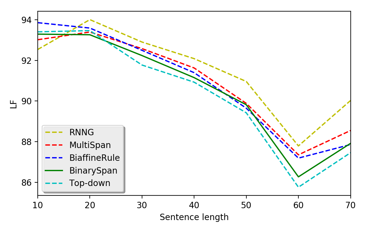
Figure 3: Sentence length v.s LF scores.

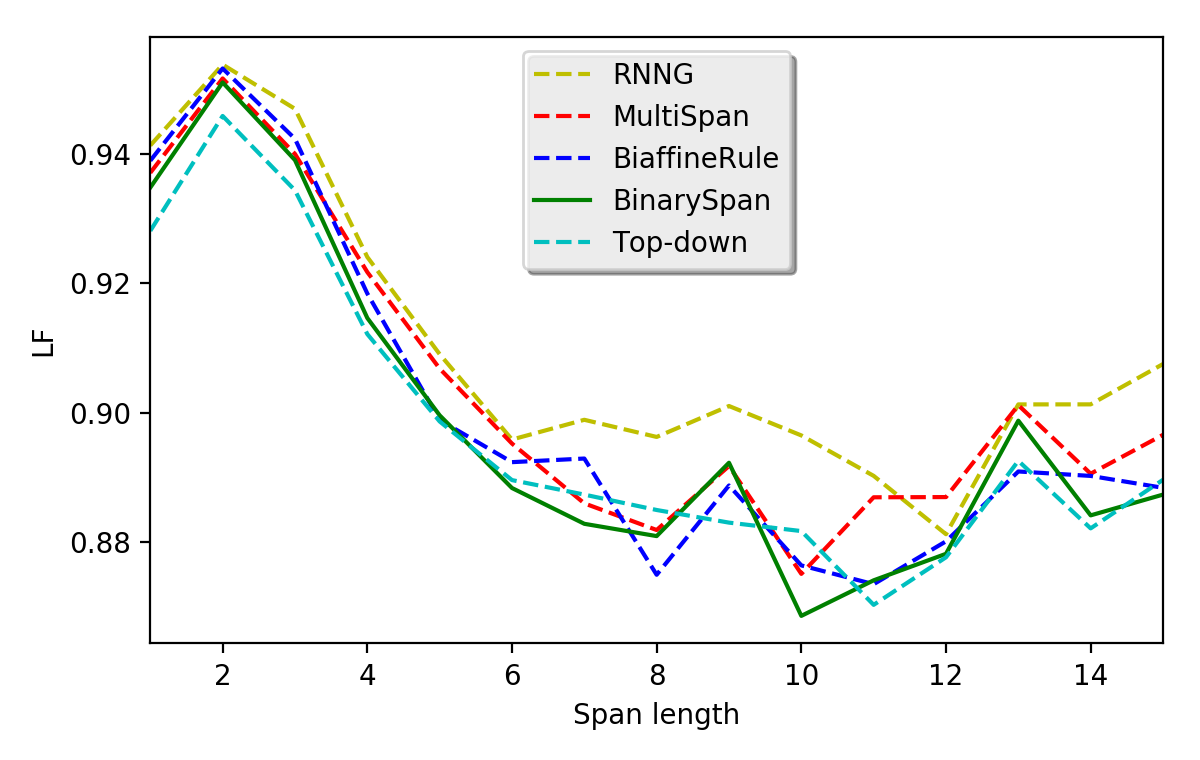
Figure 4: Span length v.s LF scores.

Model	NP	VP	S	PP	SBAR	ADVP	ADJP	WHNP	QP
BinarySpan	93.35	93.26	92.55	89.58	88.59	85.85	76.86	95.87	89.57
MultiSpan	93.61	93.41	92.76	89.96	89.16	86.39	78.21	95.98	89.51
BiaffineRule	93.53	93.46	92.78	89.30	89.56	85.89	77.47	96.66	90.31

Table 6: LF scores for major constituent labels.

Model	UF	LF	Speed(sents/s)
BinarySpan	92.16	96.79	22.12
MultiSpan	92.50	97.03	21.55
BiaffineRule	92.22	97.12	6.00

Table 7: UF, oralce LF and speed.

5 Related Work

Globally trained discriminative models have given highly competitive accuracies on graph-based constituent parsing. The key is to explicitly consider connections between output substructures in order to avoid label bias. State-of-the-art statistical methods use a single model to score a feature representation for all phrase-structure rules in a parse tree [Taskar et al. (2004, Finkel et al. (2008, Carreras et al. (2008]. More sophisticated features that span over more than one rule have been used for reranking [Huang (2008b]. ?) used neural networks to augment manual indicator features for CRF parsing. Structured learning has been used for transition-based constituent parsing also [Sagae and Lavie (2005, Zhang and Clark (2009, Zhang and Clark (2011, Zhu et al. (2013], and neural network models have been used to substitute indicator features for transition-based parsing [Watanabe and Sumita (2015, Dyer et al. (2016, Goldberg et al. (2014, Kiperwasser and Goldberg (2016b, Cross and Huang (2016a, Coavoux and Crabbé (2016, Shi et al. (2017].

Compared to the above methods on constituent parsing, our method does not use global structured learning, but instead learns local constituent patterns, relying on a bi-directional LSTM encoder for capturing non-local structural relations in the input. Our work is inspired by the biaffine dependency parser of ?). Similar to our work, ?) show that a model that bi-partitions spans locally can give high accuracies under a highly-supervised setting. Compared to their model, we build direct local span classification and CFG rule classification models instead of using span labeling and splitting features to learn a margin-based objective. Our results are better although our models are simple. In addition, they collapse unary chains as fixed patterns while we handle them with an encoder-decoder model.

6 Conclusion

We investigated two locally trained span-level constituent parsers using BiLSTM encoders, demonstrating empirically the strength of the local models on learning syntactic structures. On standard evaluation, our models give the best results among existing neural constituent parsers without external parses.

References

- [Abney (1991] Steven P. Abney. 1991. Parsing by chunks. In Principle-based parsing, pages 257–278. Springer.
- [Andor et al. (2016] Daniel Andor, Chris Alberti, David Weiss, Aliaksei Severyn, Alessandro Presta, Kuzman Ganchev, Slav Petrov, and Michael Collins. 2016. Globally normalized transition-based neural networks. In Proceedings of the 54th Annual Meeting of the Association for Computational Linguistics (Volume 1: Long Papers), pages 2442–2452, Berlin, Germany, August. Association for Computational Linguistics.
- [Bohnet (2010] Bernd Bohnet. 2010. Top accuracy and fast dependency parsing is not a contradiction. In Proceedings of the 23rd International Conference on Computational Linguistics (Coling 2010), pages 89–97, Beijing, China, August. Coling 2010 Organizing Committee.
- [Carreras et al. (2008] Xavier Carreras, Michael Collins, and Terry Koo. 2008. Tag, dynamic programming, and the perceptron for efficient, feature-rich parsing. In Proceedings of the Twelfth Conference on Computational Natural Language Learning, pages 9–16. Association for Computational Linguistics.
- [Charniak and Johnson (2005] Eugene Charniak and Mark Johnson. 2005. Coarse-to-fine n-best parsing and maxent discriminative reranking. In Proceedings of the 43rd Annual Meeting of the Association for Computational Linguistics (ACL’05), pages 173–180, Ann Arbor, Michigan, June. Association for Computational Linguistics.
- [Charniak (2000] Eugene Charniak. 2000. A maximum-entropy-inspired parser. In Proceedings of the 1st North American chapter of the Association for Computational Linguistics conference, pages 132–139. Association for Computational Linguistics.
- [Cho et al. (2014] Kyunghyun Cho, Bart Van Merriënboer, Dzmitry Bahdanau, and Yoshua Bengio. 2014. On the properties of neural machine translation: Encoder-decoder approaches. arXiv preprint arXiv:1409.1259.
- [Choe and Charniak (2016] Do Kook Choe and Eugene Charniak. 2016. Parsing as language modeling. In Proceedings of the 2016 Conference on Empirical Methods in Natural Language Processing, pages 2331–2336, Austin, Texas, November. Association for Computational Linguistics.
- [Clevert et al. (2015] Djork-Arné Clevert, Thomas Unterthiner, and Sepp Hochreiter. 2015. Fast and accurate deep network learning by exponential linear units (elus). CoRR, abs/1511.07289.
- [Coavoux and Crabbé (2016] Maximin Coavoux and Benoit Crabbé. 2016. Neural greedy constituent parsing with dynamic oracles. In Proceedings of the 54th Annual Meeting of the Association for Computational Linguistics (Volume 1: Long Papers), pages 172–182, Berlin, Germany, August. Association for Computational Linguistics.
- [Collins (2003] Michael Collins. 2003. Head-driven statistical models for natural language parsing. Computational linguistics, 29(4):589–637.
- [Cross and Huang (2016a] James Cross and Liang Huang. 2016a. Incremental parsing with minimal features using bi-directional lstm. In Proceedings of the 54th Annual Meeting of the Association for Computational Linguistics (Volume 2: Short Papers), pages 32–37, Berlin, Germany, August. Association for Computational Linguistics.
- [Cross and Huang (2016b] James Cross and Liang Huang. 2016b. Span-based constituency parsing with a structure-label system and provably optimal dynamic oracles. In Proceedings of the 2016 Conference on Empirical Methods in Natural Language Processing, pages 1–11, Austin, Texas, November. Association for Computational Linguistics.
- [Dozat and Manning (2016] Timothy Dozat and Christopher D. Manning. 2016. Deep biaffine attention for neural dependency parsing. CoRR, abs/1611.01734.
- [Durrett and Klein (2015] Greg Durrett and Dan Klein. 2015. Neural crf parsing. In Proceedings of the 53rd Annual Meeting of the Association for Computational Linguistics and the 7th International Joint Conference on Natural Language Processing (Volume 1: Long Papers), pages 302–312, Beijing, China, July. Association for Computational Linguistics.
- [Dyer et al. (2016] Chris Dyer, Adhiguna Kuncoro, Miguel Ballesteros, and Noah A. Smith. 2016. Recurrent neural network grammars. In Proceedings of the 2016 Conference of the North American Chapter of the Association for Computational Linguistics: Human Language Technologies, pages 199–209, San Diego, California, June. Association for Computational Linguistics.
- [Fernández-González and Martins (2015] Daniel Fernández-González and André F. T. Martins. 2015. Parsing as reduction. In Proceedings of the 53rd Annual Meeting of the Association for Computational Linguistics and the 7th International Joint Conference on Natural Language Processing (Volume 1: Long Papers), pages 1523–1533, Beijing, China, July. Association for Computational Linguistics.
- [Finkel et al. (2008] Jenny Rose Finkel, Alex Kleeman, and Christopher D. Manning. 2008. Efficient, feature-based, conditional random field parsing. In Proceedings of ACL-08: HLT, pages 959–967, Columbus, Ohio, June. Association for Computational Linguistics.
- [Fried et al. (2017] Daniel Fried, Mitchell Stern, and Dan Klein. 2017. Improving neural parsing by disentangling model combination and reranking effects. In Proceedings of the 55th Annual Meeting of the Association for Computational Linguistics (Volume 2: Short Papers), pages 161–166, Vancouver, Canada, July. Association for Computational Linguistics.
- [Goldberg et al. (2014] Yoav Goldberg, Francesco Sartorio, and Giorgio Satta. 2014. A tabular method for dynamic oracles in transition-based parsing. Transactions of the association for Computational Linguistics, 2:119–130.
- [Hochreiter and Schmidhuber (1997] Sepp Hochreiter and Jürgen Schmidhuber. 1997. Long short-term memory. Neural computation, 9(8):1735–1780.
- [Huang and Harper (2009] Zhongqiang Huang and Mary Harper. 2009. Self-training PCFG grammars with latent annotations across languages. In Proceedings of the 2009 Conference on Empirical Methods in Natural Language Processing, pages 832–841, Singapore, August. Association for Computational Linguistics.
- [Huang et al. (2010] Zhongqiang Huang, Mary Harper, and Slav Petrov. 2010. Self-training with products of latent variable grammars. In Proceedings of the 2010 Conference on Empirical Methods in Natural Language Processing, pages 12–22, Cambridge, MA, October. Association for Computational Linguistics.
- [Huang et al. (2012] Liang Huang, Suphan Fayong, and Yang Guo. 2012. Structured perceptron with inexact search. In Proceedings of the 2012 Conference of the North American Chapter of the Association for Computational Linguistics: Human Language Technologies, pages 142–151, Montréal, Canada, June. Association for Computational Linguistics.
- [Huang (2008a] Liang Huang. 2008a. Forest reranking: Discriminative parsing with non-local features. In Proceedings of ACL-08: HLT, pages 586–594, Columbus, Ohio, June. Association for Computational Linguistics.
- [Huang (2008b] Liang Huang. 2008b. Forest reranking: Discriminative parsing with non-local features. In Proceedings of ACL-08: HLT, pages 586–594, Columbus, Ohio, June. Association for Computational Linguistics.
- [Kiperwasser and Goldberg (2016a] Eliyahu Kiperwasser and Yoav Goldberg. 2016a. Easy-first dependency parsing with hierarchical tree lstms. Transactions of the Association for Computational Linguistics, 4:445–461.
- [Kiperwasser and Goldberg (2016b] Eliyahu Kiperwasser and Yoav Goldberg. 2016b. Simple and accurate dependency parsing using bidirectional LSTM feature representations. CoRR, abs/1603.04351.
- [Klein and Manning (2003] Dan Klein and Christopher D. Manning. 2003. Accurate unlexicalized parsing. In Proceedings of the 41st Annual Meeting of the Association for Computational Linguistics, pages 423–430, Sapporo, Japan, July. Association for Computational Linguistics.
- [Koo and Collins (2010] Terry Koo and Michael Collins. 2010. Efficient third-order dependency parsers. In Proceedings of the 48th Annual Meeting of the Association for Computational Linguistics, pages 1–11, Uppsala, Sweden, July. Association for Computational Linguistics.
- [Koo et al. (2010] Terry Koo, Alexander M. Rush, Michael Collins, Tommi Jaakkola, and David Sontag. 2010. Dual decomposition for parsing with non-projective head automata. In Proceedings of the 2010 Conference on Empirical Methods in Natural Language Processing, pages 1288–1298, Cambridge, MA, October. Association for Computational Linguistics.
- [Kuncoro et al. (2017] Adhiguna Kuncoro, Miguel Ballesteros, Lingpeng Kong, Chris Dyer, Graham Neubig, and Noah A. Smith. 2017. What do recurrent neural network grammars learn about syntax? In Proceedings of the 15th Conference of the European Chapter of the Association for Computational Linguistics: Volume 1, Long Papers, pages 1249–1258, Valencia, Spain, April. Association for Computational Linguistics.
- [Lafferty et al. (2001] John Lafferty, Andrew McCallum, Fernando Pereira, et al. 2001. Conditional random fields: Probabilistic models for segmenting and labeling sequence data. In Proceedings of the eighteenth international conference on machine learning, ICML, volume 1, pages 282–289.
- [Liu and Zhang (2017a] Jiangming Liu and Yue Zhang. 2017a. In-order transition-based constituent parsing. Transactions of the Association for Computational Linguistics, 5:413–424.
- [Liu and Zhang (2017b] Jiangming Liu and Yue Zhang. 2017b. Shift-reduce constituent parsing with neural lookahead features. Transactions of the Association for Computational Linguistics, 5:45–58.
- [Ma and Hovy (2017] Xuezhe Ma and Eduard Hovy. 2017. Neural probabilistic model for non-projective mst parsing. arXiv preprint arXiv:1701.00874.
- [Marcus et al. (1993] Mitchell P Marcus, Mary Ann Marcinkiewicz, and Beatrice Santorini. 1993. Building a large annotated corpus of english: The penn treebank. Computational linguistics, 19(2):313–330.
- [Martins et al. (2010] Andre Martins, Noah Smith, Eric Xing, Pedro Aguiar, and Mario Figueiredo. 2010. Turbo parsers: Dependency parsing by approximate variational inference. In Proceedings of the 2010 Conference on Empirical Methods in Natural Language Processing, pages 34–44, Cambridge, MA, October. Association for Computational Linguistics.
- [McClosky et al. (2006] David McClosky, Eugene Charniak, and Mark Johnson. 2006. Reranking and self-training for parser adaptation. In Proceedings of the 21st International Conference on Computational Linguistics and 44th Annual Meeting of the Association for Computational Linguistics, pages 337–344, Sydney, Australia, July. Association for Computational Linguistics.
- [Neubig et al. (2017] Graham Neubig, Chris Dyer, Yoav Goldberg, Austin Matthews, Waleed Ammar, Antonios Anastasopoulos, Miguel Ballesteros, David Chiang, Daniel Clothiaux, Trevor Cohn, et al. 2017. Dynet: The dynamic neural network toolkit. arXiv preprint arXiv:1701.03980.
- [Nivre (2003] Joakim Nivre. 2003. An efficient algorithm for projective dependency parsing. In Proceedings of the 8th International Workshop on Parsing Technologies (IWPT, pages 149–160.
- [Nivre (2008] Joakim Nivre. 2008. Algorithms for deterministic incremental dependency parsing. Comput. Linguist., 34(4):513–553, December.
- [Petrov and Klein (2007] Slav Petrov and Dan Klein. 2007. Improved inference for unlexicalized parsing. In Human Language Technologies 2007: The Conference of the North American Chapter of the Association for Computational Linguistics; Proceedings of the Main Conference, pages 404–411, Rochester, New York, April. Association for Computational Linguistics.
- [Sagae and Lavie (2005] Kenji Sagae and Alon Lavie. 2005. A classifier-based parser with linear run-time complexity. In Proceedings of the Ninth International Workshop on Parsing Technology, pages 125–132. Association for Computational Linguistics.
- [Sagae and Lavie (2006] Kenji Sagae and Alon Lavie. 2006. Parser combination by reparsing. In Proceedings of the Human Language Technology Conference of the NAACL, Companion Volume: Short Papers, pages 129–132, New York City, USA, June. Association for Computational Linguistics.
- [Shi et al. (2017] Tianze Shi, Liang Huang, and Lillian Lee. 2017. Fast(er) exact decoding and global training for transition-based dependency parsing via a minimal feature set. In Proceedings of the 2017 Conference on Empirical Methods in Natural Language Processing, pages 12–23, Copenhagen, Denmark, September. Association for Computational Linguistics.
- [Shindo et al. (2012] Hiroyuki Shindo, Yusuke Miyao, Akinori Fujino, and Masaaki Nagata. 2012. Bayesian symbol-refined tree substitution grammars for syntactic parsing. In Proceedings of the 50th Annual Meeting of the Association for Computational Linguistics (Volume 1: Long Papers), pages 440–448, Jeju Island, Korea, July. Association for Computational Linguistics.
- [Socher et al. (2013] Richard Socher, John Bauer, Christopher D. Manning, and Ng Andrew Y. 2013. Parsing with compositional vector grammars. In Proceedings of the 51st Annual Meeting of the Association for Computational Linguistics (Volume 1: Long Papers), pages 455–465, Sofia, Bulgaria, August. Association for Computational Linguistics.
- [Srivastava et al. (2014] Nitish Srivastava, Geoffrey E Hinton, Alex Krizhevsky, Ilya Sutskever, and Ruslan Salakhutdinov. 2014. Dropout: a simple way to prevent neural networks from overfitting. Journal of Machine Learning Research, 15(1):1929–1958.
- [Stern et al. (2017] Mitchell Stern, Jacob Andreas, and Dan Klein. 2017. A minimal span-based neural constituency parser. In Proceedings of the 55th Annual Meeting of the Association for Computational Linguistics (Volume 1: Long Papers), pages 818–827, Vancouver, Canada, July. Association for Computational Linguistics.
- [Sutskever et al. (2014] Ilya Sutskever, Oriol Vinyals, and Quoc V Le. 2014. Sequence to sequence learning with neural networks. In Advances in neural information processing systems, pages 3104–3112.
- [Tai et al. (2015] Kai Sheng Tai, Richard Socher, and Christopher D. Manning. 2015. Improved semantic representations from tree-structured long short-term memory networks. In Proceedings of the 53rd Annual Meeting of the Association for Computational Linguistics and the 7th International Joint Conference on Natural Language Processing, pages 1556–1566, Beijing, China, July. Association for Computational Linguistics.
- [Taskar et al. (2004] Ben Taskar, Dan Klein, Mike Collins, Daphne Koller, and Christopher Manning. 2004. Max-margin parsing. In Dekang Lin and Dekai Wu, editors, Proceedings of EMNLP 2004, pages 1–8, Barcelona, Spain, July. Association for Computational Linguistics.
- [Teng and Zhang (2016] Zhiyang Teng and Yue Zhang. 2016. Bidirectional tree-structured LSTM with head lexicalization. CoRR, abs/1611.06788.
- [Vinyals et al. (2015] Oriol Vinyals, Łukasz Kaiser, Terry Koo, Slav Petrov, Ilya Sutskever, and Geoffrey Hinton. 2015. Grammar as a foreign language. In Advances in Neural Information Processing Systems, pages 2773–2781.
- [Wang and Chang (2016] Wenhui Wang and Baobao Chang. 2016. Graph-based dependency parsing with bidirectional lstm. In Proceedings of the 54th Annual Meeting of the Association for Computational Linguistics (Volume 1: Long Papers), pages 2306–2315, Berlin, Germany, August. Association for Computational Linguistics.
- [Wang and Xue (2014] Zhiguo Wang and Nianwen Xue. 2014. Joint pos tagging and transition-based constituent parsing in chinese with non-local features. In Proceedings of the 52nd Annual Meeting of the Association for Computational Linguistics (Volume 1: Long Papers), pages 733–742, Baltimore, Maryland, June. Association for Computational Linguistics.
- [Wang et al. (2015] Zhiguo Wang, Haitao Mi, and Nianwen Xue. 2015. Feature optimization for constituent parsing via neural networks. In Proceedings of the 53rd Annual Meeting of the Association for Computational Linguistics and the 7th International Joint Conference on Natural Language Processing (Volume 1: Long Papers), pages 1138–1147, Beijing, China, July. Association for Computational Linguistics.
- [Watanabe and Sumita (2015] Taro Watanabe and Eiichiro Sumita. 2015. Transition-based neural constituent parsing. In Proceedings of the 53rd Annual Meeting of the Association for Computational Linguistics and the 7th International Joint Conference on Natural Language Processing (Volume 1: Long Papers), pages 1169–1179, Beijing, China, July. Association for Computational Linguistics.
- [Xue et al. (2005] Naiwen Xue, Fei Xia, Fu-Dong Chiou, and Marta Palmer. 2005. The penn chinese treebank: Phrase structure annotation of a large corpus. Natural language engineering, 11(02):207–238.
- [Zhang and Clark (2009] Yue Zhang and Stephen Clark. 2009. Transition-based parsing of the chinese treebank using a global discriminative model. In Proceedings of the 11th International Conference on Parsing Technologies (IWPT’09), pages 162–171, Paris, France, October. Association for Computational Linguistics.
- [Zhang and Clark (2011] Yue Zhang and Stephen Clark. 2011. Syntactic processing using the generalized perceptron and beam search. Computational linguistics, 37(1):105–151.
- [Zhang and Nivre (2011] Yue Zhang and Joakim Nivre. 2011. Transition-based dependency parsing with rich non-local features. In Proceedings of the 49th Annual Meeting of the Association for Computational Linguistics: Human Language Technologies, pages 188–193, Portland, Oregon, USA, June. Association for Computational Linguistics.
- [Zhou et al. (2015] Hao Zhou, Yue Zhang, Shujian Huang, and Jiajun Chen. 2015. A neural probabilistic structured-prediction model for transition-based dependency parsing. In Proceedings of the 53rd Annual Meeting of the Association for Computational Linguistics and the 7th International Joint Conference on Natural Language Processing (Volume 1: Long Papers), pages 1213–1222, Beijing, China, July. Association for Computational Linguistics.
- [Zhu et al. (2013] Muhua Zhu, Yue Zhang, Wenliang Chen, Min Zhang, and Jingbo Zhu. 2013. Fast and accurate shift-reduce constituent parsing. In Proceedings of the 51st Annual Meeting of the Association for Computational Linguistics (Volume 1: Long Papers), pages 434–443, Sofia, Bulgaria, August. Association for Computational Linguistics.
- [Zhu et al. (2015] Xiaodan Zhu, Parinaz Sobhani, and Hongyu Guo. 2015. Long short-term memory over recursive structures. In Proceedings of the 32nd International Conference on Machine Learning, pages 1604–1612, Lille, France, July.