Ultrafast time-resolved x-ray scattering reveals diffusive charge order dynamics in La_2-xBa_xCuO₄

Charge order is universal among high-T_c cuprates but its relevance to superconductivity is not established. It is widely believed that, while static order competes with superconductivity, dynamic order may be favorable and even contribute to Cooper pairing. We use time-resolved resonant soft x-ray scattering to study the collective dynamics of the charge order in the prototypical cuprate, La_2-xBa_xCuO₄. We find that, at energy scales $0.4$ meV $\lesssim\omega\lesssim 2$ meV, the excitations are overdamped and propagate via Brownian-like diffusion. At energy scales below 0.4 meV the charge order exhibits dynamic critical scaling, displaying universal behavior arising from propagation of topological defects. Our study implies that charge order is dynamic, so may participate tangibly in superconductivity.

One of the key questions in high temperature superconductivity is how it emerges as hole-like carriers are added to a correlated Mott insulator  (?, ?, ?). Soon after the discovery of Bednorz and Müller  (?), it was recognized that competition between kinetic energy and Coulomb repulsion could cause valence holes to segregate into periodic structures originally referred to as “stripes”  (?, ?, ?). Valence band charge order has since been observed in nearly all cuprate families  (?, ?, ?, ?, ?, ?, ?, ?, ?, ?, ?, ?), though it is not known what role, if any, charge order plays in superconductivity.

It is widely believed that, while static charge order may compete with superconductivity, fluctuating order could be favorable or even contribute to the pairing mechanism  (?, ?, ?). It is therefore crucial to determine whether the charge order in cuprates is fluctuating and, if so, what kind of dynamics it exhibits.

The generally accepted way to detect fluctuating charge order is to use energy- and momentum- resolved scattering techniques, such as inelastic x-ray or electron scattering, to measure the dynamic structure factor, $S(q,\omega)$  (?, ?). This quantity is related to the charge susceptibility, $\chi^{\prime\prime}(q,\omega)$, by the fluctuation-dissipation theorem, which asserts a quantitative relationship between the weakly nonequilibrium dynamics of a system and its equilibrium fluctuations at finite temperature  (?, ?, ?, ?). The time scale of the fluctuations can therefore be inferred from the energy dependence of the scattering data. The energy scale of charge fluctuations could, however, be of the same order as the superconducting gap, requiring instruments with sub-meV energy resolution to detect it. Such x-ray and electron spectrometers do not yet exist, calling for a different approach.

A way to achieve sub-meV energy resolution is to study the collective excitations in the time domain. The effective energy resolution of a time-resolved experiment can be defined as $\Delta\omega=2\pi\hbar/T$, where $T$ is the time interval measured  (?). Arbitrarily low energy scales can therefore be accessed by scanning to long delay times. Further, the fluctuation-dissipation theorem guarantees that the time-domain dynamics of a system may be used to shed light on its low-energy fluctuations in equilibrium.

When an ordered phase is excited out of equilibrium, its order parameter could exhibit any of several distinct types of dynamics  (?, ?, ?). For example, it might exhibit inertial dynamics, undergoing coherent oscillation around its equilibrium value at a characteristic frequency. Such dynamics are common in structural phase transitions in which the oscillation is a phonon of the distorted phase. Alternatively, the order parameter might relax back to equilibrium gradually, either through dissipation or diffusive motion of excitations. Such relaxation is influenced by conservation laws and whether continuous symmetries are present that support topological defects  (?, ?). Recent time-resolved optics studies of underdoped YBa₂Cu₃O_6+x and La_2-xSr_xCuO₄ showed coherent, meV-scale, collective oscillation of the optical response that was interpreted as an amplitude mode of the charge order  (?, ?, ?), implying dynamics of the inertial type  (?, ?). However, charge order is a finite-momentum phenomenon, while optics experiments probe the system at zero momentum, so the relationship between these oscillations and the charge order is not fully established. Analogous experiments with momentum resolution are therefore needed.

Here, we use time-resolved resonant soft x-ray scattering (tr-RSXS) to study the collective dynamics of “stripe-ordered” La_2-xBa_xCuO₄ with $x\sim 1/8$ (LBCO)  (?, ?, ?). We use 50-fs, 1.55 eV laser pulses to drive the charge order parameter out of equilibrium, and probe its subsequent dynamics by scattering 60-fs x-ray pulses from a free-electron laser (FEL) after a controlled time delay (Fig. 1A). X-ray pulses were resonantly tuned to the Cu $L_{3/2}$ edge (933 eV) and detected with either an energy-integrating avalanche photodiode (APD) or an energy-resolving soft x-ray grating spectrometer with a resolution of 0.7 eV  (?, ?). Using the latter makes this is a time-resolved RIXS (tr-RIXS) measurement and allows isolation of the resonant, valence band scattering from the Cu²⁺ fluorescence background. A total delay range of $T=40$ ps after the pump arrival was scanned with a time resolution of $\Delta t=$ 130 fs (SM, Fig. S1), allowing studies of phenomena with an energy scale ranging from $2\pi\hbar/T=0.103$ meV to $\pi\hbar/\Delta t=15.9$ meV  (?).

The LBCO crystal used in this study exhibits charge order below $T_{CO}=53$ K, which coincides with an orthorhombic-to-tetragonal structural transition  (?, ?, ?). Experiments were carried out at $T$ = 12 K ($<T_{CO}$) and focused around the charge order wave vector $\vec{Q}_{CO}=(0.23,0.00,1.50)$ r.l.u., where $(H,K,L)$ are Miller indices denoting the location of the peak in momentum space  (?, ?) (see SM, Materials and Methods for further details). For a pump fluence of 0.1 mJ/cm², the energy-integrated charge order peak, shown in Fig. 1C, is immediately suppressed due to the creation of both electron-hole pairs and the collective excitations of interest  (?, ?, ?). Fitting the momentum lineshape at each time delay with a pseudo-Voigt function (SM, section 2), we found that the peak is suppressed by 75% and broadened in momentum by 45% compared to its equilibrium profile (Figs. 1C and S3). That the peak is not fully suppressed implies the laser provided a perturbation of intermediate strength, where the original charge order has not been completely extinguished. The broadening of the peak indicates the creation of heterogeneous spatial structure in the charge order.

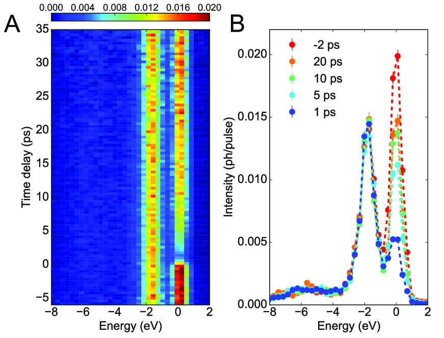
Figure 2: Time-resolved RIXS measurement of charge order in LBCO. (A) tr-RIXS spectra taken at a series of delay times with the momentum tuned to the peak of the charge order, Q_CO (data are binned in 400 fs time steps to reduce counting noise in the plot). (B) Line plots of the same tr-RIXS spectra for a selection of time delays. Error bars represent Poisson counting error. The quasielastic scattering from the charge order appears at zero energy, and is the only spectral feature influenced by the pump. The feature at -1.8 eV is a combination of $dd$ excitations and Cu²⁺ emission, and the features at -6 eV are charge transfer excitations.

It is crucial to establish whether the peak changes observed are truly properties of the valence band. Repeating the measurement using energy-resolved tr-RIXS with 0.7 eV resolution, we find that the peak suppression only takes place in the resonant, quasielastic scattering (Fig. 2). The other RIXS features, including the $dd$ and charge transfer excitations, and Cu²⁺ fluorescence emission, are unaffected by the pump. We conclude that the effects observed are properties of the valence band, and the time response will directly reveal the dynamics of the charge order.

Shortly after the pump, for time $t\lesssim 2$ ps which corresponds to an energy scale of 2 meV $\lesssim\omega\lesssim$ 15.9 meV, we observe a shift in the wave vector of the charge order peak (see Fig. 1C). This shift occurs in the scattering plane, along the $H$ momentum direction, but not along the perpendicular $K$ direction (SM, Fig. S2B). A single exponential fit to the time-dependence (Fig. 1B) indicates that the peak position recovers in $(2.13\pm 0.18)$ ps. This pump-induced phenomenon could be due to any of three effects: (1) a change in the periodicity of the charge order, (2) a change in the refractive index of the sample in the soft x-ray regime, which would alter the perceived Bragg angle of the reflection  (?), or (3) a collective recoil of the charge order condensate.

We tested the first possibility by rotating the sample azimuthal angle by 180^∘ and repeating the measurement at the same $\vec{Q}_{CO}=(0.23,0.00,1.50)$ r.l.u.. If the shift were due to a periodicity change, because the CuO₂ plane is C₄-symmetric, such a rotation would not affect the peak momentum as measured in the reference frame of the sample. Surprisingly, we found that the momentum shift reversed direction (Fig. 1B), meaning it is fixed with respect to the propagation direction of the pump, not the crystal axes. This excludes a (pure) change in the periodicity of the charge order. To test the second possibility, we measured the $(0,0,1)$ Bragg reflection of the LTT structure. A pump-induced change in the refractive index should be visible as a shift in the $(0,0,1)$ peak as well, however no such shift was observed (Fig. S6). We are led to the surprising conclusion that the pump induces a coherent recoil of the charge order condensate—in essence, a nonequilibrium population of collective modes exhibiting a nonzero center-of-mass momentum, which might be thought of as a classical Doppler shift.

To summarize so far, the initial periodic charge order is partially destroyed by the perturbing laser pulse, but by 2 ps, its amplitude is nearly restored. The next stage in its approach to equilibrium is summarized in Fig. 3A, which shows the intensity of the charge order peak for times 2 ps $\lesssim t\lesssim 10$ ps, corresponding to an energy scale of 0.4 meV $\lesssim\omega\lesssim 2$ meV. Unlike previous reports of an amplitude mode  (?, ?, ?), we see no coherent oscillation indicative of inertial dynamics. We conclude that the dynamics of the charge order in LBCO are purely relaxational, meaning its collective modes are highly damped.

Nevertheless, the excitations of the charge order propagate diffusively. In the standard description of relaxational dynamics  (?, ?) in a periodic system (see SM, section 7), a non-conserved order parameter driven weakly out of equilibrium will have a time dependence proportional to $\exp(-\gamma(q)t)$, where $q=|\vec{Q}-\vec{Q}_{CO}|$ is the momentum relative to the charge order peak and

$$\gamma(q)=\gamma_{0}+Dq^{2}.$$ (1)

Here the momentum dependence arises from diffusion quantified by the parameter, $D$ ($\gamma_{0}$ describes the dissipation). Fig. 3A shows time traces of the charge order peak intensity for $t<10$ ps for a selection of momenta $\vec{Q}$ around $\vec{Q}_{CO}$. Each curve is fit well by a single exponential, plus a constant offset that likely arises from heating of the electronic subsystem  (?) (see SM, section 6). That the curves are fit well by a single exponential implies that the charge order amplitude now deviates only weakly from its equilibrium value. We find the relaxation rate is highly momentum-dependent, increasing rapidly with $q$ (Fig. 3B), and is fit well by Eq. 1, yielding dissipation parameter $\hbar\gamma_{0}=(0.1730\pm 0.0015)$ meV and diffusion constant $\hbar D=(215\pm 19)$ meV Ų. These two quantities imply that the collective excitations of the charge order in LBCO propagate by Brownian-like diffusion, with a characteristic diffusion length $\lambda=\sqrt{2D/\gamma_{0}}\sim 50$ Å and dissipation time $1/\gamma_{0}=(3.805\pm 0.031)$ ps.

At late times, 5 ps $\lesssim t\lesssim 40$ ps, corresponding to an energy scale of 0.1 meV $\lesssim\omega\lesssim 0.8$ meV, the order parameter still exhibits relaxational dynamics, but its amplitude is nearly returned to its equilibrium value. The dynamics no longer follow a simple exponential form, but instead are characterized by self-similar dynamic scaling  (?, ?, ?, ?). The concept of dynamic scaling originated in the field of far-from-equilibrium phenomena having been observed in phase ordering dynamics of quenched binary fluids and alloys  (?, ?). The hypothesis states that the amplitude and length scale of the order parameter satisfy a universal relationship,

$$S(q,t)=L^{d}(t)F(qL(t)).$$ (2)

Here, $S(q,t)$ is the time Fourier transform of $S(q,\omega)$, $L(t)$ is the characteristic length scale of the order, and $F(x)$ is a universal function. For systems with a scalar order parameter, $L$ corresponds to the mean domain size. For systems with a continuous symmetry and a vector or tensor order parameter, $L(t)$ corresponds to the mean distance between topological defects, and increases as defects annihilate or are annealed from the system. Eq. 2 states that structure on different time scales is self-similar and independent of time if suitably scaled. Dynamic scaling only takes place at late times following a quench when the magnitude of the order parameter is large and nonlinear effects are important  (?, ?).

We found that the the late-time data can be collapsed to a single curve (Fig. 4A), using Eq. 2, taking $d=3$ and $L(t)$ as the inverse of the half-width of the charge order reflection. This collapse implies that, at sub-meV energy scales, the dynamics of the order parameter are determined by universal properties such as dimensionality and ranges of the interactions, and are not governed by any microscopic details of LBCO itself.

The behavior of $L(t)$ is sensitive to the nature of the equilibrium phase the system is approaching. If relaxing to a phase that is uniform in space, $L(t)$ is known to exhibit power law behavior at long times, $L(t)\sim t^{\alpha}$, where $\alpha=1/3$ if the order parameter is conserved and $\alpha=1/2$ if it is not  (?, ?). However, if the equilibrium phase is modulated, as is the current case of charge order in LBCO, it was predicted (for a strong quench) that the long-time behavior of two-dimensional (2D) modulated phase order is governed by the dynamics of topological defects, and $L(t)\sim\ln(t)$  (?). Such slow dynamics can arise without needing to consider additional effects due to pinning by disorder. That neighbouring layers are correlated means the topological defects behave as line defects oriented along the stacking direction, and so can be described by an effective 2D dynamics.

We test these expectations by examining the long-time ($t>10$ ps) behavior of $L(t)$. Fig. 4B shows a compensated plot seemingly indicating that $L(t)\sim t^{0.03}$ at long times. Small power laws of this sort are normally interpreted as logarithmic dependence, i.e., $L(t)\sim\ln(t)$, supporting the prediction of Ref.  (?). While disorder may be playing some role, this result is evidence that the long-time dynamics of LBCO are governed by propagation of topological defects such as dislocation lines.

Our study implies that the collective charge order excitations in LBCO are gapless down to an energy scale of 0.1 meV. The fluctuation-dissipation theorem implies that the charge order is fluctuating if maintained at any fixed temperature above 1 K. On an energy scale 0.4 meV $\lesssim\omega\lesssim 2$ meV (time scales 2 ps $\lesssim t\lesssim 10$ ps) the excitations propagate diffusively with a mean free path $\lambda\sim 50\AA$ in a mean free time $1/\gamma_{0}=(3.805\pm 0.031)$ ps. This implies that an equivalent energy-domain measurement of $S(q,\omega)$ would exhibit a featureless, quasielastic spectrum with an energy width given by $\gamma(q)$ in Fig. 3B  (?, ?) (see SM, section 7). At ultralow energy scales, 0.1 meV $\lesssim\omega\lesssim 0.4$ meV (time scales 10 ps $\lesssim t\lesssim 40$ ps) the order exhibits dynamic critical scaling, the collective excitations consisting of topological defects whose dynamics are governed by universal scaling laws independent of the microscopic details of LBCO. The dynamic nature of charge order suggests it could participate in superconductivity in a tangible way.

Supplementary materials

Materials and Methods
Supplementary Text (sections 1-7)
Figs. S1 to S8
Table S1

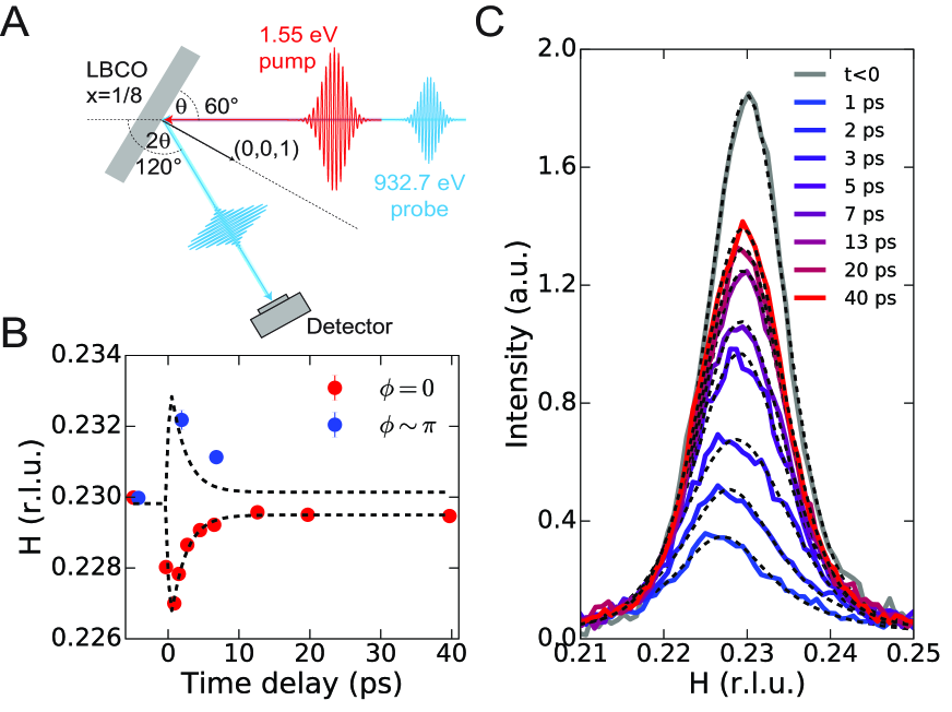
Figure 1: Pump-induced suppression and recoil of the charge order in LBCO. (A) Layout of the experiment. 1.55 eV pump pulses perturb the charge order, which is then probed by resonant scattering of co-propagating soft x-ray FEL pulses resonantly tuned to the Cu L_3/2 edge. (B) Time-dependent shift of the charge order wavevector in the $H$ momentum direction for two different azimuthal sample angles, $\phi=0$ and $\pi$. The dashed line is a fit to the $\phi=0$ data (reflected for comparison to the $\phi=\pi$ points). (C) Momentum scan in the $H$ direction through the charge order peak for a selection of time delays. Dashed lines are fits using a pseudo-Voigt function (see SM, section 2). The fluorescence background has been subtracted.

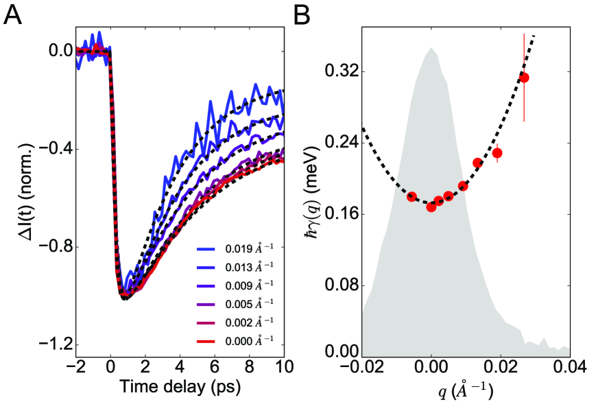
Figure 3: Collective modes of charge order in LBCO propagate diffusively. (A) (solid lines) Time traces of the energy-integrated charge order scattering for a selection of momenta $q=|\vec{Q}-\vec{Q}_{CO}|$. The data are scaled to the same height and binned into 200 fs time steps to reduce counting noise in the plot. (dashed lines) Fits using a single exponential (see SM, section 6) show the recovery time is highly momentum-dependent. (B) (red points) Exponential decay parameter, $\gamma(q)$, as a function of relative momentum difference, $q=\textrm{sgn}(H-H_{CO})|\vec{Q}-\vec{Q}_{CO}|$. Error bars represent only the statistical uncertainties in the fits. (dashed line) Fit to the data using eq. (1). (shaded area) Lineshape of the unperturbed charge order reflection in equilibrium.

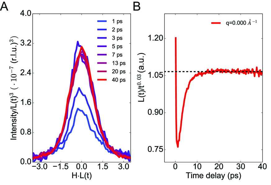
Figure 4: Demonstration of dynamic scale invariance at long times. (A) Scaled momentum profiles (as in Fig. 1C) showing that the data collapse at late times for $d=3$. Here, $L(t)$ is taken to be the inverse half-width of the reflection at each time delay, $t$. The curves have been shifted in $H$ to compensate for the momentum recoil at short times. (B) Compensated plot of the scaling function, $L(t)$, this time taken as the cube root of the peak intensity at each time delay, $t$. The data show a power law of 0.03 at long times, indicating logarithmic behavior.

Supplementary Materials for
Ultrafast time-resolved x-ray scattering reveals
diffusive charge order dynamics in La_2-xBa_xCuO₄

This PDF file includes:

• Materials and Methods

• Supplementary Text (sections 1-7)

• Figs. S1 to S8

• Table S1

Materials and Methods

Sample growth and characterization

A high-quality pellet of La_1.875Ba_0.125CuO₄ was grown by the floating zone method and cut into smaller single crystals  (?). The crystals were cleaved in air in order to expose a fresh surface, mainly oriented along the ab plane. The 2-mm-sized single crystal used in this study was pre-oriented using a lab-based Cu K$\alpha$ X-ray source. The lattice parameters were determined to be a=b=3.787 Å and c=13.23 Å . The surface miscut with respect to the ab crystalline plane was found to be 21 degrees. The superconducting T_c of the sample was verified through a SQUID magnetometry measurement to be approximately 5 K.

Time-resolved Resonant Soft X-ray Scattering

Low-temperature optical pump, soft X-ray probe measurements have been performed at the Soft X-Ray (SXR) instrument of the Linac Coherent Light Source (LCLS) X-ray free electron laser (FEL) at SLAC National Laboratory, Menlo Park, USA  (?). The measurements reported in this work were carried out at a Resonant Soft X-ray Scattering (RSXS) endstation  (?) in a $3\cdot 10^{-9}$ Torr vacuum. Low temperatures down to 12 K were achieved with a manipulator equipped with a Helium flow cryostat. Ultrafast probe X-rays at 120 Hz rep. rate were obtained by tuning the free electron laser to the Cu L_3/2 edge (931.5 eV) and with a 0.3 eV bandwidth after passing through a grating monochromator. The p-polarized X-ray pulses had a typical pulse duration of 60 fs, a pulse energy of 1.5 $\mu$J, and were focused down to a 1.5x0.03 mm² elliptical spot. The 1.55 eV optical pump pulses, also p-polarized, were generated with a Ti:sapphire amplifier run at 120 Hz and propagated collinearly with the X-rays into the RSXS endstation. The 50-fs pump was focused down to a 2.0x1.0 mm² spot in order to probe a homogeneously excited sample volume. The beams were spatially overlapped onto a frosted Ce:YAG crystal and synchronized by monitoring the reflectivity changes of a Si₃N₄ thin film. The shot-to-shot temporal jitter between pump and probe pulses was measured by means of a timing-tool  (?, ?) and corrected by time-sorting during the data analysis. The overall time resolution of approximately 130 fs was checked by measuring the crosscorrelation signal on a polished Ce:YAG crystal (see Fig. S1). Shot-to-shot intensity fluctuations from the FEL were corrected in the photodiode data through a reference intensity readout before the monochromator. The scattered X-rays were measured with an energy-integrating avalanche photodiode located on a rotating arm at 17.3 cm from the sample, while time-resolved RIXS measurements were performed with a modular qRIXS grating spectrometer  (?) mounted on a port at 135^∘ with respect to the incident beam and provided a $\sim 0.7$ eV energy resolution (FWHM) when using the 2${}^{\textrm{nd}}$ order of the grating. The spectrometer was equipped with an ANDOR CCD camera operated at 120 Hz readout rate in 1D binning mode along the non-dispersive direction. The pump-probe time delay was controlled both electronically and through a mechanical translation stage. All the time-dependent rocking curves presented in this work have been referenced to their equilibrium values by selectively varying the pump-probe time delay to negative values during the data acquisition in order to minimize errors due to motor backlash and step accuracy.

Supplementary text

1. Pump-probe cross-correlation

Fig. S1. Optical pump-X-ray probe cross-correlation. Time-sorted YAG transmittance edge measuring the cross-correlation between optical pump and soft X-rays at the sample position. The signal intensity is uncorrected for amplitude fluctuations of the FEL beam. The fit function is given in the text.

The pump-probe cross-correlation for this experiment was measured by detecting the optical transmittance of the 1.55 eV light as a function of delay w.r.t the X-ray pulse for a 0.5 mm thick polished Ce:YAG placed at the sample position using a Si photodiode (model DET36A). When interacting with the X-ray beam, the YAG transmittance at 1.55 eV exhibits a sharp edge (see Fig. S1) that can be used to characterize the global time resolution. By fitting the signal with the function $I(t)=I_{0}-\frac{\Delta I}{2}\big{[}1+\textrm{erf}\big{(}\frac{t}{\tau_{0}}\big{)}\big{]}$, we obtain a cross-correlation width $\tau_{0}=(187\pm 39)$ fs. Hence, our global time-resolution is $\tau_{0}/\sqrt{2}\sim 130$ fs under the assumption of Gaussian beam envelopes.

2. Charge order peak rocking curves fit and background subtraction

The rocking curves shown in Fig. S2 have been fitted with a pseudo-Voigt profile and a linear background,

$$I(q)\bigg{|}_{t}=(I_{0}+mq)+f\frac{1}{\pi g}\frac{A}{1+\bigg{(}\frac{q-Q_{CO}}{g}\bigg{)}^{2}}+(1-f)\frac{A}{g}\sqrt{\frac{\ln 2}{\pi}}\exp\bigg{[}-\ln 2\bigg{(}\frac{q-Q_{CO}}{g}\bigg{)}^{2}\bigg{]}$$ (3)

The first term represents the linear background, while the second and third term represent a Lorentzian and a Gaussian, respectively, with $f$ as a linear mixing parameter. The last two terms share the same amplitude parameter $A$ and the same FWHM $2g$. The fit parameters at each time delay along the H direction (Fig. S2) are reported in Fig. S3. The background slope and intercept are constant over the entire delay window, therefore a background subtraction based on the fitted slope does not introduce artifacts in the time-dependent behavior of the charge-order (CO) peak. The fit parameters in Fig. S3A-D exhibit a time dependence that can be captured by a single exponential recovery and an offset, while the background is time-independent. The same fit procedure has been also applied for the scans along the K direction shown in Fig. S2B. The fit parameters for those curves are reported in Tab. S1.

	t$<$0.0 ps	t=1.0 ps
A (a.u.)	$(14.02\pm 0.34)\cdot 10^{-3}$	$(6.35\pm 0.28)\cdot 10^{-3}$
$K_{CO}$	$(0.0\pm 0.3)\cdot 10^{-4}$	$(-7.4\pm 0.5)\cdot 10^{-4}$
g (r.l.u.)	$(4.03\pm 0.05)\cdot 10^{-3}$	$(5.23\pm 0.09)\cdot 10^{-3}$
f	$(0.655\pm 0.048)$	$(0.652\pm 0.080)$
m (r.l.u.)	$(0.00\pm 0.18)$	$(0.00\pm 0.10)$
$I_{0}$ (a.u.)	$(2.3031\pm 0.0057)$	$(2.3168\pm 0.0042)$

Table S1. Fit parameters along K projection. Pseudo-Voigt fit parameters for the curves in Fig. S2B. $K_{CO}$ is the Miller index of the $Q_{CO}$ wavevector in the fit expression.

Fig. S2. Pump-induced CO peak melting. CO peak projection along H and K for selected time delays. Solid lines are experimental data, dashed lined represent pseudo-Voigt fits.

Fig. S3. Time-dependent CO peak fit parameters. (A) Pseudo-Voigt amplitude A, (B) H projection of the CO wavevector Q, (C) CO peak HWHM g, (D) Pseudo-Voigt mixing parameter f, (E) linear background slope m (F) linear background intercept I₀. Red symbols mark the fit parameters. These points are then fit to an exponential decay in (A)-(D) (dashed grey lines) and to a constant in (E)-(F).

3. Charge order peak rocking curves for $\phi\sim\pi$

Fig. S4. CO peak shift at $\phi\sim\pi$. CO peak projection along H for selected time delays. Solid lines are experimental data, dashed lines represent pseudo-Voigt fits. Vertical dashed lines indicate the peak positions at equilibrium and at the maximum of the response. Data shown in (A) are acquired with a pump fluence of 0.2 mJ/cm² while data in (B) with 0.1 mJ/cm².

In the main text, we discuss the change in the CO peak shift direction when rotating the sample around the azimuthal angle $\phi$. In Fig. S4, we show the CO rocking curves (with background subtraction) for the blue points in Fig. 1B of the main text. These data are acquired at the same pump fluence and temperature conditions as the data reported in the rest of Fig. 1. Moreover, here we also report a second dataset exhibiting a clear peak shift when irradiated with a higher IR pump fluence.

4. Comparison between tr-RIXS and APD data

The time-dependent elastic line intensity measured with the RIXS spectrometer and integrated over the energy axis maps closely onto the time-dependent, background-subtracted CO peak intensity measurement carried out with the avalanche photodiode (see Fig. S5).

Fig. S5. Comparison between tr-RIXS and energy-integrated time dependence at Q_CO. Elastic line intensity values (energy-integrated in a 1.5-eV range around the peak) vs time delay are reported as red dots, while a rescaled, background-subtracted photodiode (APD) intensity measurement at Q_CO is shown as a solid grey line. Error bars are Poisson uncertainties.

5. Response of the LTT distortion peak

The onset of CO in 1/8-doped LBCO is accompanied by a low-temperature structural transition from a low-temperature orthorhombic (LTO) to a low-temperature tetragonal (LTT) phase  (?). This structural change allows us to observe an otherwise forbidden (0,0,1) Bragg reflection. The (0,0,1) reflection measurement is performed at resonant condition with Cu L₃ edge X-rays. Previous studies reported pump-induced changes in this peak under 1.55 eV  (?) and midinfrared  (?) irradiation and for mJ/cm² fluences. Hence it is important to check whether the structure responds as well to the excitation in the current experimental conditions. The (0,0,1) peak data at the same fluence of the CO data shown in the main text are shown in Fig. S6. The peak intensity decreases but the peak does not shift in Q, at variance with the CO diffraction signal. This is additional evidence that the lattice does not change while the charge moves.

Fig. S6. Dynamics of the LTT distortion. Projection of the (0,0,1) Bragg peak along the H direction at T=12 K for selected time delays and for a pump fluence of 0.1 mJ/cm².

6. Raw time-dependent, energy-integrated peak intensities around $Q_{CO}$

In Fig. 3A of the main text, we show normalized differential intensity changes vs pump-probe time delay. In Fig. S7 we show the unscaled intensity curves after time-sorting and rebinning with 200 fs time steps. Shot-to-shot intensity fluctuations have been corrected with a reference intensity monitor prior to the monochromator, while the fluorescence background has not been subtracted out. Each intensity curve is fit with a single exponential recovery and an offset capturing the long-time relaxation of the CO peak. The fit function for each momentum cut is

$$I(t)\Bigg{|}_{q}=\bigg{|}\Delta_{0}-\Theta(t-t_{d})\bigg{[}1-\exp\bigg{(}-\frac{t-t_{d}}{\tau_{0}}\bigg{)}\bigg{]}\bigg{[}A_{0}+A_{1}\exp\bigg{(}-\frac{t-t_{d}}{\tau}\bigg{)}\bigg{]}\bigg{|}^{2}+I_{\textrm{bkg}}.$$ (4)

In this expression, the pump-induced signal grows with an exponential saturation characterized by a timescale $\tau_{0}$. $A_{1}$ and $A_{0}$ respectively represent the exponential amplitude and an offset, while $\tau$ is the timescale of the exponential recovery. $t_{d}$ is the parameter for the zero time delay. $\Delta_{0}$ is the equilibrium value of the order parameter, while $I_{\textrm{bkg}}$ is the fluorescence contribution to the overall intensity. The fit curves are indicated in Fig. S7 as black dashed lines.

Fig. S7. Raw time-dependent CO peak intensity. Energy-integrated, time-dependent intensity profiles of the CO peak for a pump fluence of 0.1 mJ/cm² and for selected momenta (solid lines). Data are binned along the time axis in 200 fs steps to improve statistics. Single exponential fit curves are shown as dashed black lines.

7. Momentum-dependent recovery of the charge-ordered phase

The purpose of this section is to calculate the relaxation of long-wavelength fluctuations of the charge order parameter as it approaches an equilibrium periodic state, in the spirit of Landau theory. The calculation remains in the framework of the time-dependent Ginzburg-Landau equation but the coarse-grained free energy takes into account the periodic charge order state.

Our data indicate that following the application of a laser pulse, the periodic state undergoes exponential relaxation with a rate $\gamma(\textbf{q})$ in the interval 2 ps $<t<10$ ps, where q is the momentum relative to the charge order peak at $\textbf{Q}_{CO}$. Our goal is to calculate the functional form of $\gamma(\textbf{q})$, and show that it is of the form of Eq. (1) in the main text.

We model the charge density condensate as a function of space x and time $t$ by the Swift-Hohenberg equation, a widely used minimal model of periodic pattern formation  (?, ?), which has previously been used to describe charge density wave dynamics  (?). Written in canonical form it is:

$$\tau_{0}\frac{\partial\psi}{\partial t}=\epsilon\psi-{\psi}^{3}-\xi_{0}^{4}(q_{0}^{2}+\nabla^{2})^{2}\psi$$ (5)

Here $\psi=\psi(\textbf{x},t)$ is the charge order parameter rescaled so that the cubic term has coefficient unity, $\tau_{0}$ is a relaxation time, $q_{0}$ is the magnitude of the wavevector at the onset of ordering when the control parameter $\epsilon>0$ and $\xi_{0}$ is a charge fluctuation correlation length. The control parameter is determined by the degree to which the temperature is below the critical temperature for charge ordering. In the experiment, apart from the period when the system is excited by the laser, the temperature is well below the critical temperature, and we are deep into the regime where periodic charge order occurs. In principle this equation should have an additive noise that obeys the fluctuation-dissipation theorem, but this will not concern us if we restrict our calculation purely to linear stability. Note that the Swift-Hohenberg equation does not conserve the charge, and this is appropriate because it is only the total charge from the condensate and the quasi-particles that is conserved.

When $\epsilon>0$ the uniform state $\psi=0$ becomes linearly unstable to the formation of a periodic state. The wavelength of this periodic state is not unique, because there is a band of linearly stable periodic steady states around the most unstable mode with wavenumber $q_{0}$, thus posing the so-called pattern selection problem. A large body of work shows in detail how the initial and boundary conditions as well as the history of the system determine which of these possible steady states is actually chosen by the dynamics  (?), but here we simply use the observed charge order state rather than try to predict what it should be. Given that a periodic state of charge order exists, the next step is to perform the linear stability analysis around this pattern.

We assume the stripe patterns are periodic in the $x$ direction, and constant in the $y$ direction, and make a single-mode approximation:

$$\psi(\textbf{x},t)=\psi_{0}\left[A(x,y,t)e^{iq_{0}x}+c.c.\right]$$ (6)

where the slowly-varying complex amplitude $A$ can be shown to obey the equation  (?)

$$\partial_{t}A=\epsilon A+\mu_{0}^{2}\left(\partial_{x}-\frac{i}{2q_{0}}\partial_{y}^{2}\right)^{2}A-3|A|^{2}A$$ (7)

where $\mu_{0}=2q_{0}$. It is known that the single-mode approximation is qualitatively accurate and that the dependence with $\epsilon$ of the selected wave vector is weak, so we use this amplitude equation description as a first approximation to describe the long-wavelength dynamics.

Rescaling the equation by $q_{0}\rightarrow\frac{q_{0}}{\mu_{0}}$, $A\rightarrow A/\sqrt{3}$ and $\textbf{x}\rightarrow\mu_{0}\textbf{x}$, we obtain the Newell-Whitehead equation in canonical form  (?):

$$\partial_{t}A=\epsilon A+\left(\partial_{x}-\frac{i}{2q_{0}}\partial_{y}^{2}\right)^{2}A-|A|^{2}A$$ (8)

Since the wavenumber of the stripes can be anywhere within the band, and is determined through an pattern selection process that is not of concern here, we will denote the wavenumber of the actual selected stripe pattern to be $q_{0}+k$. This means that our stability analysis is around the state described by the complex amplitude

$$A_{k}=a_{k}e^{ikx},$$ (9)

where $a_{k}=\sqrt{\epsilon-k^{2}}$. We now impose a small perturbation, i.e. $A=A_{k}+\delta A$ with wavenumber $\textbf{q}=(q_{x},q_{y})$ where:

$$\delta A=(\delta a_{+}e^{i\textbf{q}\cdot\textbf{x}}+\delta a_{-}e^{-i\textbf{q}\cdot\textbf{x}})e^{ikx}$$ (10)

and the negative mode is included due to the presence in the linearized equation of the term $\delta A^{*}$.

Plugging back into the Newell-Whitehead equation, we find the linearized equations of motion:

$$\partial_{t}\delta a_{+}=-(a_{k}^{2}+U_{+})\delta a_{+}-a_{k}^{2}\delta a_{-}\\ \partial_{t}\delta a_{-}=-a_{k}^{2}\delta a_{+}-(a_{k}^{2}+U_{-})\delta a_{-}$$ (11)

where

$$U_{\pm}=(k\pm q_{x})^{2}+\frac{(\pm q_{x}+k)q^{2}_{y}}{q_{0}}-\frac{q^{4}_{y}}{4q_{0}^{2}}-k^{2}$$ (12)

By writing eq. (11) in matrix form and solving for the eigenvalues $\lambda_{\pm}$, we obtain:

$$\begin{array}[]{cl}\lambda_{\pm}&=-a_{k}^{2}-\frac{U_{+}+U_{-}}{2}\pm\sqrt{a_{k}^{4}+\frac{(U_{+}-U_{-})^{2}}{4}}\\ &=-\epsilon+k^{2}-q_{x}^{2}-\frac{kq_{y}^{2}}{q_{0}}+\frac{q_{y}^{4}}{4q_{0}^{2}}\pm\sqrt{(\epsilon-k^{2})^{2}+4k^{2}q_{x}^{2}+\frac{4kq_{x}^{2}q_{y}^{2}}{q_{0}}+\frac{q_{x}^{2}q_{y}^{4}}{q_{0}^{2}}}\\ &\simeq-\epsilon+k^{2}-q_{x}^{2}\pm\sqrt{(\epsilon-k^{2})^{2}+4k^{2}q_{x}^{2}}\\ &\simeq-\epsilon+k^{2}-q_{x}^{2}\pm\left[(\epsilon-k^{2})+\frac{2k^{2}q_{x}^{2}}{\epsilon-k^{2}}\right]\end{array}$$ (13)

In the scattering geometry of our experiment, sketched in Fig. S8, $q_{y}\ll q_{x}$ so that we find to a good approximation

$$\lambda_{+}=-\frac{\epsilon-3k^{2}}{\epsilon-k^{2}}q_{x}^{2},\qquad\lambda_{-}=-2(\epsilon-k^{2})-\frac{\epsilon+k^{2}}{\epsilon-k^{2}}q_{x}^{2}$$ (14)

Fig. S8. Schematic representation of the scattering geometry. For the purpose of this section, the xy plane is defined as parallel to the CuO₂ planes. The scattering plane lies orthogonal to the stripe direction, here denoted as y. $k_{i}$ and $k_{f}$ represent the incident and scattered momenta of the x-ray beam, $Q_{CO}$ is the charge order wavevector described in the main text and $q$ is the small momentum deviation from $Q_{CO}$ considered in this section.

The mode with eigenvalue $\lambda_{+}$ is a Goldstone phase mode that in the limit of vanishing $q_{x}$ restores translational invariance. It is likely not to be present in our system because of disorder or grain boundaries between the stripe domains, both of which break translational invariance.

The mode with eigenvalue $\lambda_{-}$ is a decaying mode that corresponds to that measured in Fig. 3B of the main text. We conclude by rewriting it in the physical units. The $x$-component of the measured charge order wavevector is $Q_{CO}=q_{0}+k$ and $k\rightarrow k\cdot 2q_{0}\cdot\xi_{0}^{2}$. Since q is defined relative to the charge order wavevector, we have that $q=q_{x}+O(q_{y}/q_{x})\approx q_{x}$. Further neglecting the dependence of $k$ on $\epsilon$ leads to the simple formulae for the decay rate extracted from the experiment:

$$\gamma(q)=2\epsilon+q^{2}$$ (15)

or in the original units:

$$\gamma(q)=\frac{2\epsilon}{\tau_{0}}+\frac{(2q_{0}\xi_{0}^{2})^{2}}{\tau_{0}}q^{2}.$$ (16)

This result is Eq. (1) of the main text.

References

- 1. S. A. Kivelson, E. Fradkin, V. J. Emery, Nature 393, 550 (1998).
- 2. M. Vojta, Adv. Phys. 58, 699 (2009).
- 3. B. Keimer, S. A. Kivelson, M. R. Norman, S. Uchida, J. Zaanen, Nature 518, 179 (2015).
- 4. J. G. Bednorz, K. A. Müller, Z. Phys. B: Condens. Matter 64, 189–193 (1986).
- 5. K. Machida, Physica C 158, 192 (1986).
- 6. H. J. Schulz, J. Phys. France 50, 2833 (1986).
- 7. J. Zaanen, O. Gunnarsson, Phys. Rev. B 40, R7391 (1986).
- 8. J. M. Tranquada, et al., Nature 429, 534 (2004).
- 9. P. Abbamonte, et al., Nature Physics 1, 155 (2005).
- 10. S. A. Kivelson, E. Fradkin, Handbook of High-Temperature Superconductivity, J. R. Schrieffer, J. S. Brooks, eds. (Springer Science, 233 Spring Street, New York, NY 10013, USA, 2007), chap. 15, pp. 570–592.
- 11. G. Ghiringhelli, et al., Science 337, 821 (2012).
- 12. R. Comin, et al., Science 343, 390 (2014).
- 13. E. H. da Silva Neto, et al., Science 343, 393 (2014).
- 14. M. Le Tacon, et al., Nature Physics 7, 725 (2011).
- 15. J. Chang, et al., Nature Physics 8, 871 (2012).
- 16. E. Berg, E. Fradkin, S. A. Kivelson, Phys. Rev. B 79, 064515 (2009).
- 17. E. Fradkin, S. A. Kivelson, J. M. Tranquada, Reviews of Modern Physics 87, 457 (2015).
- 18. S. Gerber, et al., Science 350, 949 (2015).
- 19. M. H. Hamidian, et al., Nature 532, 343 (2016).
- 20. S. A. Kivelson, et al., Rev. Mod. Phys. 75, 1201 (2003).
- 21. D. Pines, P. Noziéres, The Theory of Quantum Liquids, Advanced Book Classics (Perseus Books, Cambridge, Massachussets, USA, 1966).
- 22. L. D. Landau, E. M. Lifshitz, Physical Kinetics, Course of Theoretical Physics (Pergamon Press Ltd., Headington Hill Hall, Oxford OX3 0BW, England, 1981).
- 23. N. Goldenfeld, Lectures on Phase Transitions and the Renormalization Group, Frontiers in Physics (Westview Press, 5500 Central Ave., 80301 Boulder, CO, USA, 1992).
- 24. P. M. Chaikin, T. C. Lubensky, Principles of Condensed Matter Physics (Cambridge University Press, University printing House, Cambridge CB2 8BS, UK, 1995).
- 25. P. Abbamonte, et al., Proc. Natl. Acad. Sci. 105, 12159 (2008).
- 26. D. H. Torchinsky, F. Mahmood, A. T. Bollinger, I. Božović, N. Gedik, Nature Materials 12, 387 (2013).
- 27. G. L. Dakovski, et al., Physical Review B 91, 220506 (2015).
- 28. J. P. Hinton, et al., Physical Review B 88, 060508 (2013).
- 29. M. Hücker, et al., Physical Review B 83, 104506 (2011).
- 30. D. Doering, et al., Review of Scientific Instruments 82, 073303 (2011).
- 31. Y. D. Chuang, et al., Review of Scientific Instruments 88, 013110 (2017).
- 32. M. Först, et al., Physical Review Letters 112, 157002 (2014).
- 33. V. Khanna, et al., Phys. Rev. B 93, 224522 (2016).
- 34. W. S. Lee, et al., Nature Communications 3, 838 (2012).
- 35. S. Smadici, J. C. T. Lee, G. Logvenov, I. Bozovic, P. Abbamonte, J. Phys.: Condens. Matter 26, 025303 (2013).
- 36. L. Perfetti, et al., Rev. Mod. Phys. 49, 435 (1977).
- 37. A. J. Bray, Adv. Phys. 51, 481 (2002).
- 38. M. Mondello, N. D. Goldenfeld, Phys. Rev. A 42, 5865 (1990).
- 39. M. Mondello, N. D. Goldenfeld, Phys. Rev. A 45, 657 (1992).
- 40. S. Vogelgesang, et al., Nature Phys. 14, 184 (2017).
- 41. Y. C. Chou, I. Goldburg, Phys. Rev. A 23, 858 (1981).
- 42. B. D. Gaulin, S. Spooner, Y. Morii, Physical Review Letters 59, 668 (1987).
- 43. T. Nagaya, H. Orihara, Y. Ishibashi, Journal of the Physical Society of Japan 64, 78 (1995).
- 44. Q. Hou, S. Sasa, N. Goldenfeld, Physica A: Statistical Mechanics and its Applications 239, 219 (1997).
- 45. W. F. Schlotter, et al., Review of Scientific Instruments 83, 043107 (2012).
- 46. H. T. Lemke, et al., SPIE Optics + Optoelectronics, T. Tschentscher, K. Tiedtke, eds. (SPIE, 2013), pp. 87780S–5.
- 47. M. Harmand, et al., Nature Photonics 7, 215 (2013).
- 48. J. Swift, P. Hohenberg, Physical Review A 15, 319 (1977).
- 49. M. Cross, P. Hohenberg, Reviews of Modern Physics 65, 851 (1993).
- 50. M. Karttunen, M. Haataja, K. Elder, M. Grant, Physical Review Letters 83, 3518 (1999).
- 51. A. Newell, J. Whitehead, Journal of Fluid Mechanics 38, 279 (1969).