Studying the [OIII]$\lambda$5007Å emission-line width in a sample of $\sim$80 local active galaxies: A surrogate for $\sigma_{\star}$?

Abstract

For a sample of $\sim$80 local ($0.02\leq z\leq 0.1$) Seyfert-1 galaxies with high-quality long-slit Keck spectra and spatially-resolved stellar-velocity dispersion ($\sigma_{\star}$) measurements, we study the profile of the [OIII]$\lambda$5007Å emission line to test the validity of using its width as a surrogate for $\sigma_{\star}$. Such an approach has often been used in the literature, since it is difficult to measure $\sigma_{\star}$ for type-1 active galactic nuclei (AGNs) due to the AGN continuum outshining the stellar-absorption lines. Fitting the [OIII] line with a single Gaussian or Gauss-Hermite polynomials overestimates $\sigma_{\star}$ by 50-100%. When line asymmetries from non-gravitational gas motion are excluded in a double Gaussian fit, the average ratio between the core [OIII] width ($\sigma_{\rm{[OIII],D}}$) and $\sigma_{\star}$ is $\sim$1, but with individual data points off by up to a factor of two. The resulting black-hole-mass-$\sigma_{\rm{[OIII],D}}$ relation scatters around that of quiescent galaxies and reverberation-mapped AGNs. However, a direct comparison between $\sigma_{\star}$ and $\sigma_{\rm{[OIII],D}}$ shows no close correlation, only that both quantities have the same range, average and standard deviation, probably because they feel the same gravitational potential. The large scatter is likely due to the fact that line profiles are a luminosity-weighted average, dependent on the light distribution and underlying kinematic field. Within the range probed by our sample (80-260 km s^-1), our results strongly caution against the use of [OIII] width as a surrogate for $\sigma_{\star}$ on an individual basis. Even though our sample consists of radio-quiet AGNs, FIRST radio-detected objects have, on average, a $\sim$10% larger [OIII] core width.

1 Introduction

The relationship between the masses of supermassive black holes (BHs) and the properties of their host galaxies has been amongst the most active research areas in contemporary astrophysics, hinting at a co-evolution between BHs and galaxies (for a recent review see, e.g., Kormendy & Ho, 2013). Such a co-evolution can be explained either by mutual growth via mergers or by feedback from the active galactic nucleus (AGN) in an evolutionary stage when the BH is growing through accretion. AGNs are thus promising probes towards understanding the origin of these BH mass ($M_{\rm BH}$) scaling relations. Unfortunately, the AGN emission (featureless non-stellar continuum plus emission lines) often outshines the host galaxy, making it difficult to measure the host-galaxy properties. In particular, measuring stellar-velocity dispersion ($\sigma_{\star}$), which, of all host galaxy properties, seems to scale the tightest with the BH mass (Beifiori et al., 2012; Shankar et al., 2016), is hampered by the contaminating AGN continuum and emission lines.

To mitigate this problem, several studies have suggested to use the width of the [OIII]$\lambda$5007Å emission line (hereafter [OIII]) originating in the narrow-line region (NLR) as a surrogate for $\sigma_{\star}$, assuming that the NLR is gravitationally bound to the bulge and thus, that the gas kinematics follows the bulge potential (e.g., Terlevich et al., 1990; Whittle, 1992; Nelson & Whittle, 1996; Nelson, 2000; Shields et al., 2003; Boroson, 2003; Greene & Ho, 2005; Netzer & Trakhtenbrot, 2007; Salviander et al., 2007, 2013). However, while the [OIII] emission line is a prominent line that can be easily measured in AGNs out to large distances, it is also known to often have asymmetric line profiles due to non-gravitational gas kinematics such as outflows, infalls, or interaction with radio jets. In particular, it is known to often display a blue wing (e.g., Heckman et al., 1981; De Robertis & Osterbrock, 1984; Whittle, 1985; Wilson & Heckman, 1985; Mullaney et al., 2013; Woo et al., 2016), generally interpreted as a signature of outflows with dust preferentially hiding one cone behind the stellar disk. For that reason, some studies have excluded the [OIII] blue wing, as well as any radio sources and galaxies undergoing tidal interactions. The $M_{\rm BH}$ was found to scale with the width of the [OIII] line ($\sigma_{\rm{[OIII]}}$), albeit with a large scatter (e.g., Nelson & Whittle, 1996; Greene & Ho, 2005). Other studies have suggested the use of different emission lines, such as [SII]$\lambda\lambda$6716, 6731 (e.g., Komossa & Xu, 2007; Ho, 2009) that have a lower ionization potential and do not suffer from substantial asymmetries, or mid-infrared lines (e.g., Dasyra et al., 2008, 2011), but the scatter is comparable to that of the core of the [OIII] line. While all studies confirm the original findings by Nelson & Whittle (1996), i.e. a moderately strong correlation between $\sigma_{\star}$ and $\sigma_{\rm{[OIII]}}$ but with real scatter, the origin of the scatter remains unclear. No dependencies have been found with AGN luminosity, host galaxy morphology, star formation rate, or local environment (Greene & Ho, 2005; Rice et al., 2006).

However, unlike the original study by Nelson & Whittle (1996), very few previous studies have measured both properties, $\sigma_{\star}$ and $\sigma_{\rm{[OIII]}}$, directly and simultaneously for a given sample, mainly due to the difficulties of measuring stellar-velocity dispersion in type-1 active galaxies. Often, conclusions are instead drawn by comparing the $M_{\rm BH}$-$\sigma_{\rm{[OIII]}}$ relation for type-1 galaxies to the $M_{\rm BH}$-$\sigma_{\star}$ relation for quiescent galaxies (Nelson, 2000; Komossa & Xu, 2007), or by comparing $M_{\rm BH}$ derived from $\sigma_{\rm{[OIII]}}$ to $M_{\rm BH}$ derived from reverberation mapping (Nelson, 2000) or the virial method using H$\beta$ (Boroson, 2003). Bonning et al. (2005) predict $\sigma_{\star}$ indirectly from the Faber-Jackson relation and conclude, from studying the $M_{\rm host}$-$\sigma_{\rm{[OIII]}}$ relationship for a sample of 21 radio-quiet quasars, that $\sigma_{\rm{[OIII]}}$ is on average consistent with $\sigma_{\star}$. Similarly, Salviander et al. (2015) find agreement with the Faber-Jackson relation when using the width of the [OIII] emission line as a proxy for stellar-velocity dispersion, supporting the general utility of the [OIII] line width as a surrogate for $\sigma_{\star}$ in statistical studies. Grupe & Mathur (2004) and Wang & Lu (2001) use $\sigma_{\rm{[OIII]}}$ to investigate their $M_{\rm BH}$ distributions of narrow-line Seyfert-1 galaxies (NLSy1). Greene & Ho (2005) compare $\sigma_{\rm{[OIII]}}$ to $\sigma_{\star}$ directly, but for a sample of type-2 Seyfert galaxies. Similarly, Woo et al. (2016) use a sample of 39,000 type-2 AGNs at $z<0.3$ from SDSS and find a broad relation between [OIII] and $\sigma_{\star}$, but with [OIII] being wider by 30-40% since wings are not excluded from the fit. However, for a sub-sample of AGNs for which the [OIII] profile is well fitted by a single Gaussian model, Woo et al. (2016) find that the velocity dispersion is comparable to the stellar-velocity dispersion. Rice et al. (2006) use spatially-resolved HST/STIS spectra for a sample of mostly type-2 Seyfert galaxies and find that NLR line widths underestimate $\sigma_{\star}$. Other studies have assumed that $\sigma_{\rm{[OIII]}}$ traces $\sigma_{\star}$ and used it to probe cosmic evolution (Shields et al., 2003; Salviander et al., 2013). Also, most studies cited above use the width of the entire [OIII] emission line, possibly including non-gravitational motion, even though already Nelson & Whittle (1996) showed that the [OIII] line profile base and wings do not correlate as tightly with stellar-velocity dispersion as the [OIII] core (similar conclusions were also reached by Greene & Ho, 2005).

Thus, despite the widespread use of $\sigma_{\rm{[OIII]}}$ as a substitute for $\sigma_{\star}$, caution is in order.

We have recently presented a baseline of the $M_{\rm BH}$-$\sigma_{\star}$ relation for active galaxies for a sample of 65 Seyfert-1 galaxies in the local Universe selected from the Sloan Digital Sky Survey (SDSS) (Bennert et al., 2015). SDSS images are used to determine host-galaxy morphology and AGN luminosity free of host-galaxy contamination. High signal-to-noise ratio Keck spectra yield H$\beta$ line width to estimate $M_{\rm BH}$ and spatially-resolved stellar-velocity dispersion (Bennert et al., 2011a; Harris et al., 2012). Thus, our sample is uniquely suited to study the direct relationship between $\sigma_{\star}$ and $\sigma_{\rm{[OIII]}}$ for a homogeneous sample of local Seyfert-1 galaxies. Moreover, we make use of the spatially-resolved Keck spectra to isolate the nuclear line profile and to probe spatial dependencies. We compare the resulting $M_{\rm BH}$-$\sigma_{\rm{[OIII]}}$ relation to the $M_{\rm BH}$-$\sigma_{\star}$ relation (Bennert et al., 2015) and look for trends with host galaxy and nuclear properties.

The paper is organized in the following manner. Section 2 summarizes the sample selection, observations, and data reduction. Section 3 describes the analysis of the data. Section 4 discusses the derived quantities and results. Section 5 concludes with a summary. Note that the paper presents, first, a traditional approach focused on velocity dispersion ratios and their correlations to $M_{\rm BH}$, and then discusses the correlation between kinematic estimators directly and the shortcomings of conclusions based solely on ratios. Throughout the paper, a Hubble constant of H₀ = 70 km s^-1, $\Omega_{\rm{\lambda}}$ = 0.7, and $\Omega_{\rm{M}}$ = 0.3 are assumed.

2 Sample Selection, Observations, and Data Reduction

Sample selection, observations, and data reduction are described in detail in previous papers, in which we are focusing on the BH mass scaling relations for this sample (Bennert et al., 2011a; Harris et al., 2012; Bennert et al., 2015). In brief, 102 type-1 Seyfert galaxies were selected from the SDSS data release six (DR6) based on redshift (0.02 $\leq z\leq$ 0.1) and $M_{\rm BH}$ ($>10^{7}M_{\odot}$). They were observed with the Low Resolution Imaging Spectrometer (LRIS) at the Keck 10-m telescope between January 2009 and March 2010, using a 1" wide, 175" long slit aligned with the major axis of the host galaxy (as determined from SDSS images), with exposure times ranging from 600 to 1200 s. Here, we use only the blue spectra, covering a range of $\sim$3200-5350Å and an instrumental resolution of 88 km s^-1 ($R\simeq 3000$). The instrumental resolution of our aperture spectra was determined from the [OI] 5577Å atmospheric emission line as the square root of the second moment (which is approximately FWHM/2.355 for a Gaussian) and subtracted in quadrature from the width measurements.

Data were reduced following standard reduction steps (bias subtraction, flat field correction, cosmic ray rejection, wavelength calibration, and relative flux calibration). Spatially-resolved spectra were extracted at the center of each galaxy and offset in either direction along the major axis (see Harris et al., 2012, for more details). We make use of these spatially-resolved spectra to compare $\sigma_{\star}$ (Harris et al., 2012) to the [OIII] line-width ($\sigma_{\rm{[OIII]}}$) at different distances from the nucleus. For each galaxy, we extracted the central spectrum plus up to five spectra on either side of the center (out to 5"), giving a total of 11 spectra. However, not all spectra were used for all galaxies, depending on the S/N, available $\sigma_{\star}$ measurement in Harris et al. (2012) and presence of the [OIII] emission line. Additionally, we also use aperture spectra within the bulge effective radius, as determined in Bennert et al. (2015), resulting in one additional spectrum per galaxy. We also included the [OII]$\lambda$3727Å line (hereafter [OII]) in this comparison. However, given that the [OII] line is much weaker than the [OIII] line in these AGN-powered spectra, we can only fit the [OII] line for the central row, as well as within the effective radius. Our final sample consists of 81 galaxies for which we have at least one $\sigma_{\rm{[OIII]}}$ measurement.

3 Analysis

3.1 Fits to [OIII]

To fit the emission lines around [OIII], a multi-component spectral decomposition code is used (described in detail in Park et al. (2015)). The continuum is modeled by a combination of AGN featureless non-stellar continuum, AGN Fe II emission template (Boroson & Green, 1992), and host galaxy starlight templates from the Indo-US spectral library (Valdez et al., 2004). The broad H$\beta$ emission line is fitted by Gauss-Hermite polynomials (order 3-6) (van der Marel & Franx, 1993; Woo et al., 2006; McGill et al., 2008). The [OIII]$\lambda\lambda$4959,5007Å emission lines are fitted keeping their flux ratio fixed at 1:3. The [OIII]$\lambda$5007Å fit is used as a template for the narrow H$\beta$, with the flux ratio as a free parameter. For examples of fits to the central spectra for the entire region around H$\beta$, see Bennert et al. (2015).

Three different approaches are used to fit [OIII]$\lambda$5007Å: (1) a single Gaussian is fitted, with the resulting width being referred to in the following as $\sigma_{\rm[OIII],S}$; (2) a double Gaussian is fitted, with the resulting width of the central component only being referred to in the following as $\sigma_{\rm[OIII],D}$; (3) a Gauss-Hermite polynomial series (order 7-12) is fitted, with the second moment of the full distribution (i.e., the line dispersion) referred to as $\sigma_{\rm[OIII],GH}$. The reasoning for the choice of these three fits is as follows.

If the cause for the line broadening is Doppler motion of the line emitting gas, a Gaussian profile is expected. While a single Gaussian can yield a reasonable fit in cases without line asymmetries, asymmetries are known to occur especially for the [OIII] emission line (e.g., Heckman et al., 1981; De Robertis & Osterbrock, 1984; Whittle, 1985; Wilson & Heckman, 1985). Gauss-Hermite polynomials can give the best fit to the overall line profile. However, in case of asymmetries, we expect both the single Gaussian as well as Gauss-Hermite polynomials to overestimate the width of the central [OIII] component. This core component is the one we are interested in since it is the one emitted from gas most likely to follow the gravitational potential of the bulge. To isolate this component from gas motion, such as outflows and infalls reflected in blue or red wings, we use a double Gaussian fit. In some objects, the second Gaussian is used to fit an underlying broader central component, indicating turbulent motion (Kollatschny & Zetzl, 2013). When comparing the derived width to the stellar-velocity dispersion, we only consider the Gaussian fitting of the central core component, i.e. the Gaussian with the higher peak and smaller width.

A single Gaussian is fitted for a total of 346 spectral rows, a Gauss-Hermite polynomial for 336 spectral rows and a double Gaussian for 326 spectral rows. Note that, in cases of low S/N, fitting the line with a double Gaussian can result in the wing component fitting noise. We thus carefully inspected all fits by eye and excluded those cases. It is generally recommended to only fit with a double Gaussian in cases of clear evidence of a broader wing component and/or to enforce a peak-to-noise level of the second component of at least 3 (see also, Woo et al., 2016). In addition to S/N, spectral resolution is also important when fitting a double Gaussian. A resolution much smaller than $R\simeq 3000$, as is used here, would make this approach challenging.

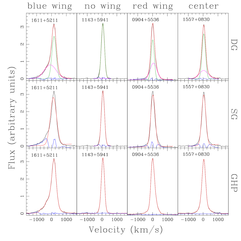
Figure 1: Illustration of [OIII] fitting methods. Three objects are shown: in the first column, the [OIII] emission line of object 1611+5211 has a blue wing; in the second column, the [OIII] emission line of object 1143+5941 has no distinct wing; in the third column, the [OIII] emission line of object 0904+5536 has a red wing; in the fourth column, the [OIII] emission line of object 1557+0830 has a broader central component. The different [OIII] emission lines are fitted by a double Gaussian (DG; upper panels), a single Gaussian (SG; middle panels) and a Gauss-Hermite polynomial function (GHP; lower panels). The observed spectrum is shown in black, the total fit is in red. For the double Gaussian fit, the green line shows one Gaussian fitted to the central core [OIII] emission line, the magenta line shows one Gaussian fitted to the blue/red wing or broader central component. While a single Gaussian is only a good fit for lines without asymmetries (such as 1143+5941), the Gauss-Hermite polynomials give the best overall fit to the line. However, both the single Gaussian and the Gauss-Hermite polynomial fits overestimate the line width of the central core [OIII] emission line.

Figure 1 illustrates our approach. Tables 1-3 list the results.

Table 1: Sample and quantities within effective bulge radius. Col. (1): target ID used throughout the text (based on R.A. and declination). Col. (2): Right ascension. Col. (3): Declination. Col. (4): Redshift from SDSS-DR7. Col. (5): Logarithm of BH mass (solar units) (uncertainty of 0.4 dex). Col. (6): Spheroid effective radius in kpc. Col. (7): Stellar-velocity dispersion within spheroid effective radius determined from CaH&K (uncertainty of 0.04 dex). Col. (8): [OIII] width within spheroid effective radius determined from double Gaussian fit (central line only; uncertainty of 0.04 dex). Col. (9): [OIII] width within spheroid effective radius determined from single Gaussian fit (uncertainty of 0.04 dex). Col. (10): [OIII] width within spheroid effective radius determined from Gauss-Hermite polynomial fit (uncertainty of 0.04 dex). Col. (11): [OII] width within spheroid effective radius (uncertainty of 0.04 dex). Note that objects with “no data” in some of the columns are not included in Bennert et al. (2015) since one of the quantities for the BH mass - $\sigma_{\star}$ relationship could not be determined, but at least some spatially-resolved $\sigma_{\star}$ measurements exist in Harris et al. (2012) and these objects are included in the spatially-resolved [OIII] measurements in Table 3. Col. (12): FIRST integrated radio flux. ND = not detected. NC = not covered, that is outside of the survey area.

Object	R.A.	Decl.	$z$	log $M_{\rm BH}$/$M_{\odot}$	$r_{\rm eff,sph}$	$\sigma_{\rm\star}$	$\sigma_{\rm[OIII],D}$	$\sigma_{\rm[OIII],S}$	$\sigma_{\rm[OIII],GH}$	$\sigma_{\rm[OII]}$	FIRST
	(J2000)	(J2000)			(kpc)	(km s-1)	(km s-1)	(km s-1)	(km s-1)	(km s-1)	(mJy)
(1)	(2)	(3)	(4)	(5)	(6)	(7)	(8)	(9)	(10)	(11)	(12)
0013$-$0951	00 13 35.38	$-$09 51 20.9	0.0615	7.85	4.8	96	123	212	261	151	ND
0026+0009	00 26 21.29	+00 09 14.9	0.0600	7.05	1.8	172	190	190	193	171	ND
0038+0034	00 38 47.96	+00 34 57.5	0.0805	8.23	1.9	127	174	212	249	160	1.67
0109+0059	01 09 39.01	+00 59 50.4	0.0928	7.52	0.3	183	144	263	310	175	1.09
0121$-$0102	01 21 59.81	$-$01 02 24.4	0.0540	7.75	1.8	90	152	247	290	205	4.00
0150+0057	01 50 16.43	+00 57 01.9	0.0847	7.25	4.5	176	131	174	245	149	ND
0206$-$0017	02 06 15.98	$-$00 17 29.1	0.0430	8.00	6.2	225	183	229	307	165	ND
0212+1406	02 12 57.59	+14 06 10.0	0.0618	7.32	1.0	171	152	181	223	158	NC
0301+0110	03 01 24.26	+01 10 22.8	0.0715	…	…	…	…	…	…	…	ND
0301+0115	03 01 44.19	+01 15 30.8	0.0747	7.55	2.7	99	144	312	375	114	ND
0336$-$0706	03 36 02.09	$-$07 06 17.1	0.0970	7.53	12.9	236	138	188	230	238	ND
0353$-$0623	03 53 01.02	$-$06 23 26.3	0.0760	7.50	1.6	175	113	155	177	131	ND
0735+3752	07 35 21.19	+37 52 01.9	0.0962	…	…	…	…	…	…	…	ND
0737+4244	07 37 03.28	+42 44 14.6	0.0882	7.55	4.2	…	…	…	…	…	1.01
0802+3104	08 02 43.40	+31 04 03.3	0.0409	7.43	2.8	116	…	…	…	…	ND
0811+1739	08 11 10.28	+17 39 43.9	0.0649	7.17	2.5	142	103	124	138	111	ND
0813+4608	08 13 19.34	+46 08 49.5	0.0540	7.14	1.0	122	100	116	145	109	ND
0831+0521	08 31 07.62	+05 21 05.9	0.0635	…	…	…	…	…	…	…	1.73
0845+3409	08 45 56.67	+34 09 36.3	0.0655	7.37	1.4	123	89	121	179	103	ND
0857+0528	08 57 37.77	+05 28 21.3	0.0586	7.42	2.5	126	124	156	194	124	ND
0904+5536	09 04 36.95	+55 36 02.5	0.0371	7.77	4.0	194	144	173	216	155	1.35
0909+1330	09 09 02.35	+13 30 19.4	0.0506	…	…	…	…	…	…	…	ND
0921+1017	09 21 15.55	+10 17 40.9	0.0392	7.45	2.6	…	109	161	211	109	ND
0923+2254	09 23 43.00	+22 54 32.7	0.0332	7.69	0.9	149	158	275	316	285	9.29
0923+2946	09 23 19.73	+29 46 09.1	0.0625	7.56	4.2	142	102	117	151	119	ND
0927+2301	09 27 18.51	+23 01 12.3	0.0262	6.94	7.1	196	172	198	241	185	2.79
0932+0233	09 32 40.55	+02 33 32.6	0.0567	7.44	0.7	126	121	152	169	131	ND
0932+0405	09 32 59.60	+04 05 06.0	0.0590	…	…	…	…	…	…	…	ND
0938+0743	09 38 12.27	+07 43 40.0	0.0218	…	…	…	…	…	…	…	ND
0948+4030	09 48 38.43	+40 30 43.5	0.0469	…	…	…	…	…	…	…	ND
1002+2648	10 02 18.79	+26 48 05.7	0.0517	…	…	…	…	…	…	…	ND
1029+1408	10 29 25.73	+14 08 23.2	0.0608	7.86	3.0	185	163	182	224	179	1.33
1029+2728	10 29 01.63	+27 28 51.2	0.0377	6.92	2.6	112	133	169	213	142	ND
1029+4019	10 29 46.80	+40 19 13.8	0.0672	7.68	2.0	166	170	210	266	168	ND
1042+0414	10 42 52.94	+04 14 41.1	0.0524	7.14	3.2	…	133	157	207	135	ND
1049+2451	10 49 25.39	+24 51 23.7	0.0550	8.03	1.3	162	141	161	209	160	ND
1058+5259	10 58 28.76	+52 59 29.0	0.0676	7.50	1.3	122	116	152	187	145	ND
1101+1102	11 01 01.78	+11 02 48.8	0.0355	8.11	5.8	197	161	224	253	232	2.86
1104+4334	11 04 56.03	+43 34 09.1	0.0493	7.04	1.1	…	108	155	203	127	ND
1116+4123	11 16 07.65	+41 23 53.2	0.0210	7.23	1.6	108	149	174	252	162	2.27
1118+2827	11 18 53.02	+28 27 57.6	0.0599	…	…	…	…	…	…	…	ND
1137+4826	11 37 04.17	+48 26 59.2	0.0541	6.74	1.1	155	152	241	257	175	2.71
1140+2307	11 40 54.09	+23 07 44.4	0.0348	…	…	…	…	…	…	…	ND
1143+5941	11 43 44.30	+59 41 12.4	0.0629	7.51	3.8	122	111	119	150	124	ND
1144+3653	11 44 29.88	+36 53 08.5	0.0380	7.73	1.0	168	120	190	229	151	ND
1145+5547	11 45 45.18	+55 47 59.6	0.0534	7.22	1.4	118	136	201	241	156	ND
1147+0902	11 47 55.08	+09 02 28.8	0.0688	8.39	3.4	147	151	175	204	178	1.15
1205+4959	12 05 56.01	+49 59 56.4	0.0630	8.00	2.4	152	175	217	244	202	1.79
1206+4244	12 06 26.29	+42 44 26.1	0.0520	…	…	…	…	…	…	…	ND
1210+3820	12 10 44.27	+38 20 10.3	0.0229	7.80	0.6	141	133	179	200	150	5.88
1223+0240	12 23 24.14	+02 40 44.4	0.0235	7.10	3.4	124	120	170	198	181	ND
1228+0951	12 28 11.41	+09 51 26.7	0.0640	…	…	…	…	…	…	…	ND
1231+4504	12 31 52.04	+45 04 42.9	0.0621	7.32	1.5	169	205	306	417	229	5.56
1241+3722	12 41 29.42	+37 22 01.9	0.0633	7.38	1.7	144	132	174	212	184	ND

Table 2: Table 1 continued.

Object	R.A.	Decl.	$z$	log $M_{\rm BH}$/$M_{\odot}$	$r_{\rm eff,sph}$	$\sigma_{\rm\star}$	$\sigma_{\rm[OIII],D}$	$\sigma_{\rm[OIII],S}$	$\sigma_{\rm[OIII],GH}$	$\sigma_{\rm[OII]}$	FIRST
	(J2000)	(J2000)			(kpc)	(km s-1)	(km s-1)	(km s-1)	(km s-1)	(km s-1)	(mJy)
(1)	(2)	(3)	(4)	(5)	(6)	(7)	(8)	(9)	(10)	(11)	(12)
1246+5134	12 46 38.74	+51 34 55.9	0.0668	6.93	3.9	119	116	132	162	148	ND
1250$-$0249	12 50 42.44	$-$02 49 31.5	0.0470	…	…	…	…	…	…	…	ND
1306+4552	13 06 19.83	+45 52 24.2	0.0507	7.16	2.3	114	122	161	212	117	ND
1312+2628	13 12 59.59	+26 28 24.0	0.0604	7.51	1.7	109	103	126	217	113	ND
1313+3653	13 13 48.96	+36 53 57.9	0.0667	…	…	…	…	…	…	…	ND
1323+2701	13 23 10.39	+27 01 40.4	0.0559	7.45	0.9	124	158	219	276	184	ND
1353+3951	13 53 45.93	+39 51 01.6	0.0626	…	…	…	…	…	…	…	ND
1405$-$0259	14 05 14.86	$-$02 59 01.2	0.0541	7.04	0.6	125	132	189	235	106	ND
1416+0137	14 16 30.82	+01 37 07.9	0.0538	7.26	3.6	173	182	291	342	211	1.70
1419+0754	14 19 08.30	+07 54 49.6	0.0558	8.00	5.4	215	211	285	354	187	4.49
1423+2720	14 23 38.43	+27 20 09.7	0.0639	…	…	…	…	…	…	…	ND
1434+4839	14 34 52.45	+48 39 42.8	0.0365	7.66	0.9	109	132	178	207	150	ND
1535+5754	15 35 52.40	+57 54 09.3	0.0304	8.04	2.8	110	175	208	244	147	5.32
1543+3631	15 43 51.49	+36 31 36.7	0.0672	7.73	3.8	146	140	221	257	218	ND
1545+1709	15 45 07.53	+17 09 51.1	0.0481	8.03	1.1	163	143	172	225	153	ND
1554+3238	15 54 17.42	+32 38 37.6	0.0483	7.87	1.7	158	200	235	287	217	2.52
1605+3305	16 05 02.46	+33 05 44.8	0.0532	7.82	1.6	187	122	128	137	120	ND
1606+3324	16 06 55.94	+33 24 00.3	0.0585	7.54	1.7	157	192	226	263	155	ND
1611+5211	16 11 56.30	+52 11 16.8	0.0409	7.67	1.3	116	152	259	349	182	3.67
1636+4202	16 36 31.28	+42 02 42.5	0.0610	7.86	9.7	205	197	227	314	130	1.18
1655+2014	16 55 14.21	+20 14 42.0	0.0841	…	…	…	…	…	…	…	ND
1708+2153	17 08 59.15	+21 53 08.1	0.0722	8.20	8.1	231	182	238	306	405	ND
2221$-$0906	22 21 10.83	$-$09 06 22.0	0.0912	7.77	6.1	142	126	154	198	134	ND
2222$-$0819	22 22 46.61	$-$08 19 43.9	0.0821	7.66	1.7	122	208	464	500	209	4.22
2233+1312	22 33 38.42	+13 12 43.5	0.0934	8.11	2.1	193	160	257	303	196	NC
2327+1524	23 27 21.97	+15 24 37.4	0.0458	7.52	6.6	225	133	271	335	173	NC
2351+1552	23 51 28.75	+15 52 59.1	0.0963	8.08	2.5	186	101	232	245	254	NC

Table 3: Spatially-resolved quantities. Col. (1): Target ID used throughout the text (based on R.A. and declination). Col. (2): Offset of spatially resolved spectrum from center. Col. (3): Spatially resolved stellar-velocity dispersion determined from CaH&K (uncertainty of 0.04 dex) taken from Harris et al. (2012). Col. (4): Spatially resolved [OIII] width determined from double Gaussian fit (central line only; uncertainty of 0.04 dex). Col. (5): Spatially resolved [OIII] width determined from single Gaussian fit (uncertainty of 0.04 dex). Col. (6): Spatially resolved [OIII] width determined from Gauss-Hermite polynomial fit (uncertainty of 0.04 dex). This table is available in its entirety in machine-readable form in the online journal. A portion is shown here for guidance regarding its form and content.

Object	Offset	$\sigma_{\rm\star}$	$\sigma_{\rm[OIII],D}$	$\sigma_{\rm[OIII],S}$	$\sigma_{\rm[OIII],GH}$
	arcsec	(km s-1)	(km s-1)	(km s-1)	(km s-1)
(1)	(2)	(3)	(4)	(5)	(6)
0013$-$0951	+0.00	113	131	222	299
0013$-$0951	+0.68	135	131	215	281
0013$-$0951	+1.62	…	313	378	520
0013$-$0951	$-$0.68	119	169	236	340
0013$-$0951	$-$1.62	162	386	392	612

3.2 Fits to [OII]

The [OII]$\lambda$3727Å emission line is really a blended doublet line of [OII]$\lambda$3726,3729ÅÅ. It is a line with a lower ionization potential (13.6 eV compared to 35 eV for [OIII]), emitted at larger distances from the nucleus and, as such, spectra are expected to be less complex and dominated by rotation. ([OIII] emitted from closer in can be more affected by outflows and winds from the accretion disk, e.g.) We thus fitted the line with a double Gaussian centered on the doublet, forcing both lines to have the same width, but leaving the ratio as a free parameter since it depends on electron density. We used the resulting width (of a single Gaussian) as $\sigma_{\rm[OII]}$. However, the [OII] line is weaker than the [OIII] line and can only be fitted for the central row as well as within the effective radius.

3.3 Stellar-velocity dispersion

Spatially-resolved stellar-velocity dispersion measurements were taken from Bennert et al. (2011a) and Harris et al. (2012), stellar-velocity dispersion measurements within the bulge effective radius (determined from surface photometry fitting of SDSS images) from Bennert et al. (2015, their equation (1)). For details, including examples of the fits, we refer the reader to those papers. In short, $\sigma_{\star}$ was measured from three different spectral regions, around CaH&K$\lambda$$\lambda$3969, 3934Å (hereafter CaH&K), around the Mg Ib$\lambda$$\lambda$$\lambda$5167, 5173, 5184Å (hereafter MgIb) lines and around Ca II$\lambda$$\lambda$$\lambda$8498, 8542, 8662Å (hereafter CaT), fitting a linear combination of Gaussian-broadened template spectra (G and K giants of various temperatures as well as spectra of A0 and F2 giants from the Indo-US survey) and a polynomial continuum using a Markov chain Monte Carlo (MCMC) routine, following van der Marel (1994). We used the resulting $\sigma_{\star}$ from the CaT region, if available, else from CaH&K and finally from MgIb, if the two former were not available.

4 Results and Discussion

We here compare the resulting widths for [OIII] and [OII] with $\sigma_{\star}$. All 81 objects have at least one $\sigma_{\rm{[OIII]}}$ measurement. Quantities necessary for comparison of $\sigma_{\rm{[OIII]}}$ and $\sigma_{\star}$ for aperture spectra within the effective bulge radius are available for 62 of the 81 objects and, thus, the $M_{\rm BH}$-$\sigma_{\rm{[OIII]}}$ relation is compared directly to the M_BH-$\sigma_{\star}$ relation for that sub-sample of 62 objects (Bennert et al., 2015). Likewise, when including $\sigma_{\rm[OII]}$ within the effective radius in the comparison, a total of 62 objects are compared.

4.1 [OIII] profile

The double Gaussian fit reveals information on the general [OIII] line profile. For 66% of objects/spectral rows, the double Gaussian fitting resulted in the fitting of a blue wing (-500 km s^-1 $\leq$ $v$ $\leq$ -25 km s^-1). For 22% of objects/spectral rows, a Gaussian redshifted compared to the central core was fitted, implying a red wing (25 km s^-1 $\leq$ $v$ $\leq$ 500 km s^-1). For 12% of objects/rows, the second Gaussian fitted a broader central component (-25 km s^-1 $\leq$ $v$ $\leq$ 25 km s^-1).

The histogram of the velocity offset of the second Gaussian (the wing component) compared to the central core Gaussian is shown in Figure 2, including all objects and spectral rows. The average velocity offset for the blue wing is -155$\pm$7 km s^-1, and for the red wing 124$\pm$13 s^-1, respectively. While these results are overall comparable with those of Woo et al. (2016) for a sample of $\sim$39,000 type-2 AGNs in SDSS, we find an even higher fraction of kinematic signatures for outflows, likely because of the type-1 nature of our objects for which the viewing angle is favorable to see outflows. Indeed, the average [OIII] profile for type-1 AGNs, as determined from a sample of $\sim$10,000 AGNs from SDSS, shows a strong blue wing that can be well fitted by a broad second Gaussian component (average velocity offset of -148 km s^-1) (Mullaney et al., 2013). Figure 3 shows examples of the broadest and the narrowest [OIII] emission line profile.

The [OIII] line shows rotation in at least 17% of objects with rotational velocities up to $\sim$$\pm$250 km s^-1, matching those of the stellar rotation curve (Harris et al., 2012). In 15% of objects do we see evidence for HII regions in the outer spectra, as traced by a sudden peak in [OIII] along with an increase in the H$\beta$/[OIII] ratio. However, since H$\alpha$ is not covered by our spectra, we cannot verify the origin of the ionization of these regions and thus do not further discuss them here. There is a small fraction of objects ($\sim$7%) that shows evidence for a change in the [OIII] profile as a function of distance from the center, with the majority showing a red wing on one side of the galaxy center and a blue wing on the other, and some galaxies with the blue wing only present on one side of the galaxy center (Figure 4).

Other than that, we do not find any trends with distance from the center. For example, the ratio of broad (wing) [OIII] to narrow (core) [OIII] does not change significantly as a function of radius (when fitted by a double Gaussian); nor does the width of the broad [OIII] component change with radius. Part of this is likely due to the fact that (i) the spectra are restricted to the central few kpc, given the S/N ratio, and (ii) that the central 1-2 kpc are unresolved due to the ground-based seeing. (The 1" width of the long-slit was chosen to match the seeing. 1" corresponds to 0.43kpc for the smallest redshift of z=0.021 of our sample, to 1.8kpc for the largest redshift of z=0.097, and to 1.1kpc for the average redshift of z=0.058.)

Figure 2: Histogram of the velocity offset of the second Gaussian (the wing component) compared to the central core Gaussian for all objects and spectral rows.

Figure 3: Examples of central [OIII] profiles for broadest [OIII] line (2222-0819, $\sigma_{\rm[OIII],GH}$ = 514 km s^-1) and narrowest [OIII] line (1605+3305, $\sigma_{\rm[OIII],GH}$ = 127 km s^-1). For comparison, the local continuum was subtracted and the peak flux scaled to 1.

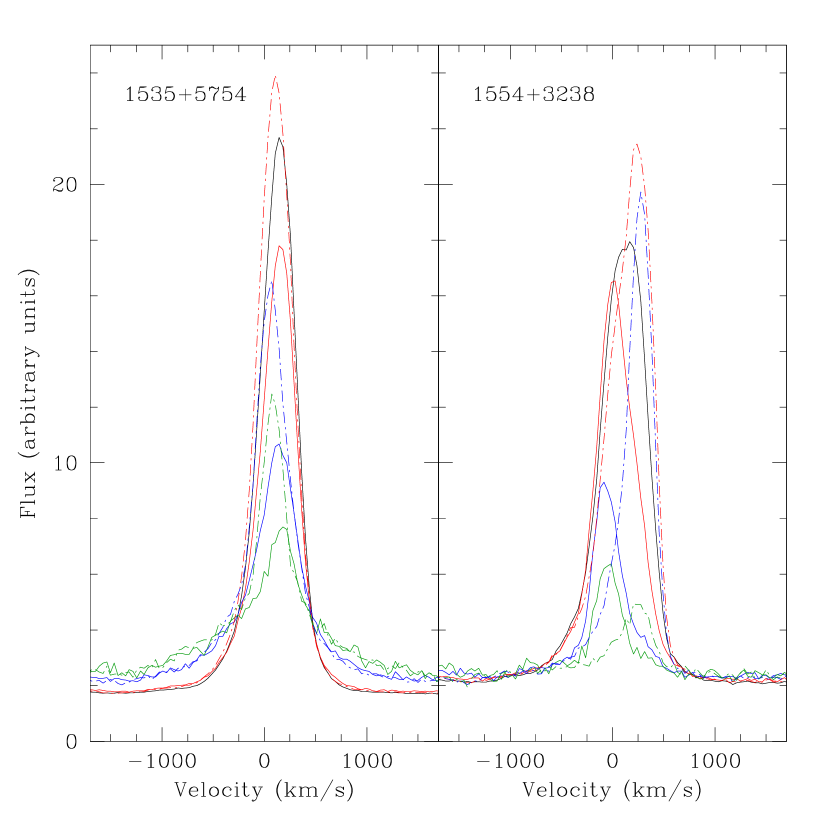
Figure 4: Examples of two objects that show a spatially changing [OIII] emission line profile (center = black; “negative” offset from center = solid lines; “positive” offset from center = dash-dotted lines; red = 0.68” distance; blue = 1.62” distance; green = 2.84” distance). Left: 1535+5754, observed at a position angle (p.a.) of 100deg, with broader lines further out from the center (“negative”=south-east). This galaxy does not show a strong rotation curve (Bennert et al., 2011a). Right: 1554+3238, observed at a p.a. of 80deg. In addition to the rotation curve ($\pm$200km/s) also visible from the stellar-absorption lines (Bennert et al., 2011a), the object shows a blue wing on the “positive” side of the center (south-east) and a red wing on the “negative” side (north-west).

4.2 Comparison between [OIII] line width and $\sigma_{\star}$

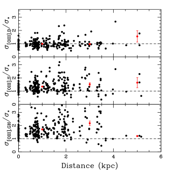
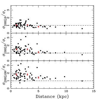
Figure 5: Ratio of [OIII] width ($\sigma_{\rm[OIII]}$) to stellar-velocity dispersion ($\sigma_{\star}$) as function of distance from galaxy center. Left: for spatially-resolved spectra. Right: for aperture spectra integrated over effective bulge radius. Red data points show average ratio within distance bins 0-2 kpc, 2-4 kpc and 4-6 kpc (4-10 kpc for right panel), respectively.

We compare the [OIII] line width ($\sigma_{\rm[OIII]}$) derived from the three different fitting methods (single Gaussian, double Gaussian using the central core component only, and Gauss-Hermite polynomials) with the stellar-velocity dispersion ($\sigma_{\star}$). In Figure 5, the resulting $\sigma_{\rm[OIII]}$/$\sigma_{\star}$ ratio is shown as a function of distance from the center for both the spatially resolved spectra (left panels) as well as the aperture spectra within the bulge effective radius (right panels). In summary, the results show that both the single Gaussian fit as well as the Gauss-Hermite polynomial fit result in an overestimation of $\sigma_{\star}$ by on average 50-100% (see Table 4). In other words, the entire [OIII] line is broader by $\sim$75% compared to $\sigma_{\star}$. However, when line asymmetries are fitted by a second Gaussian and excluded, then the central core [OIII] emission-line width is a good tracer of $\sigma_{\star}$ (mean ratio 1.06$\pm$0.02 for spatially-resolved spectra; mean ratio 1.02$\pm$0.04 for spectra within aperture of effective radius ), but with individual data points off by up to a factor of two.

Another approach to exclude line asymmetries would be to consider only the width (i.e., $\sigma$) of the first pure Gaussian term in the Gauss-Hermite polynomial fit. Note that the first term (an original symmetric Gaussian) can represent most of the core of the line profile, while the rest of the series (Gaussian multiplied by Hermite polynomials) represents deviations to better describe the observed data profile. The resulting mean ratio with $\sigma_{\star}$ is then reduced to 1.25$\pm$0.04. While this is significantly lower than using the width (i.e., line dispersion) of the full profile of the fit, it still overestimates $\sigma_{\star}$ by $\sim$25%. This is likely due to the fact that the higher order series terms can have negative values which might then be compensated for by the Gaussian, resulting in an overestimation of the width by the Gaussian component (see also, Woo et al., 2018).

Within the uncertainties, our data do not show a strong dependency of the $\sigma_{\rm[OIII]}$/$\sigma_{\star}$ on distance from the galactic center for any of the three fitting methods. At first sight, this might indicate that the influence of outflows is not necessarily more dominant in the central regions. However, given the S/N ratio, we do not probe regions outside the central few kpc. Moreover, given the ground-based seeing of $\sim$1-1.5$\arcsec$ of these Keck long-slit spectra and given the redshift range of our sample, the central 1-2 kpc are essentially unresolved (as mentioned above).

We probe the dependency of the $\sigma_{\rm[OIII]}$/$\sigma_{\star}$ ratio on the velocity offset of the second Gaussian, the wing component, with respect to the central core Gaussian component (using the spatially resolved data). For the majority of the objects and rows, the [OIII] profile has a blue wing (see previous section). Fitting this wing with a separate Gaussian results in $\sigma_{\rm[OIII],D}$/$\sigma_{\star}$ = 1.06$\pm$0.02. For objects/rows with a red wing, the core component $\sigma$ ratio is $\sigma_{\rm[OIII],D}$/$\sigma_{\star}$ = 1.01$\pm$0.03. For objects/rows for which the second Gaussian component fitted a broader underlying central component, $\sigma_{\rm[OIII],D}$/$\sigma_{\star}$ = 1.05$\pm$0.06. However, in all three cases, if these non-gravitational kinematic (blueshifted/redshifted/broad central) components are not excluded from the fit by a second Gaussian, they result in an overestimation of $\sigma_{\star}$. For a single Gaussian fit, $\sigma_{\star}$ is overestimated by 50$\pm$4% for blueshifted wings, by 45$\pm$7% for redshifted wings, and by 49$\pm$8% for central broadening. A Gauss-Hermite Polynomial leads to an overestimation of 92$\pm$5% for blue wings, 94$\pm$10% for red wings and 82$\pm$12% for broader central components. This shows the necessity of fitting a double Gaussian for all types of [OIII] profiles (blue wing, red wing or broader center) and considering only the narrow core component as a surrogate for $\sigma_{\star}$.

We also checked for dependencies of the $\sigma_{\rm[OIII]}$/$\sigma_{\star}$ ratio on the velocity shift of the entire [OIII] profile compared to the H$\beta$ absorption line from stars. The only noticeable trend is that a handful of objects/rows with large $\sigma_{\rm[OIII]}$/$\sigma_{\star}$ ratio in the core [OIII] (as fitted by the double Gaussian) are among those with large blueshifted [OIII] lines with an offset of at least -150 km s^-1. However, while [OIII] can be offset by -300 km s^-1 to 200 km s^-1, there is no strong trend between the velocity shift and the $\sigma_{\rm[OIII]}$/$\sigma_{\star}$ ratio, regardless of fitting method.

The width of the [OIII] wing (when fitted by a double Gaussian) is larger by an average factor of 2.95$\pm$0.06 compared to the [OIII] core, without showing a trend with distance from the center or overall velocity shift of the [OIII] line with respect to the H$\beta$ absorption line. This result is consistent with Woo et al. (2016) for a sample of $\sim$39,000 type-2 AGNs from SDSS.

To look for a possible physical origin of the scatter, we test dependencies of the $\sigma_{\rm[OIII]}$/$\sigma_{\star}$ ratio on other AGN and host-galaxy parameters, taken from our previous publications (Bennert et al., 2015; Runco et al., 2016). In particular, we probe the relationship between the $\sigma_{\rm[OIII]}$/$\sigma_{\star}$ ratio and BH mass, as well as $L_{5100}$ luminosity, but do not find a relationship. Likewise, there is no correlation between the $\sigma_{\rm[OIII]}$/$\sigma_{\star}$ ratio and the [OIII]/H$\beta_{\rm narrow}$ flux ratio, host-galaxy morphology, or host-galaxy inclination. This is in line with results by Rice et al. (2006) who also did not find any trends in residuals when compared to host galaxy and nuclear properties. While our sample consists of radio-quiet objects, we discuss the effect of radio jets further below.

Note that while integral-field spectroscopic studies have found increasing evidence of galaxies with kinematically de-coupled stellar and gaseous components with fractions as large as $\sim$30-40% in elliptical and lenticular galaxies (see e.g., Sarzi et al., 2006; Davis et al., 2011; Barrera-Ballesteros et al., 2015, and references therein), the larger survey of MaNGA finds only 5% of kinematically misaligned galaxies (Jin et al., 2016). Moreover, out of these, 90% reside in early-type galaxies. Given our sample of pre-dominantly late-type galaxies ($\sim$77% with host galaxies classified as Sa or later; Bennert et al. 2015), we expect a negligible fraction of kinematically de-coupled galaxies in our sample. Indeed, the overall gas rotation curve (as traced by [OIII]) matches that of the stellar rotation curve (Harris et al., 2012), with rotational velocities up to $\sim$$\pm$250 km s^-1.

Table 4: Ratios of [OIII] width to stellar-velocity dispersion depending on fitting method and distance from center. Col. (1): Extraction of spectra. Col. (2): Fitting method of [OIII] emission line. Col. (3): Mean and uncertainty (of the mean) of the resulting ratio of [OIII] width ($\sigma_{\rm[OIII]}$) to stellar-velocity dispersion ($\sigma_{\star}$) for all measurements. Col. (4): Same as Col. (3), but for distance from center of 0-2 kpc. Col. (5): Same as Col. (3), but for distance from center of 2-4 kpc. Col. (6): Same as Col. (3), but for distance from center of 4-6 kpc (4-10 kpc in case of reff).

Spectrum	[OIII] Fit	Mean Ratio	Mean Ratio	Mean Ratio	Mean Ratio
		Total	Bin 1	Bin 2	Bin 3
(1)	(2)	(3)	(4)	(5)	(6)
Spatially resolved	Double Gaussian	1.06$\pm$0.02	1.06$\pm$0.02	1.03$\pm$0.04	1.4$\pm$0.3
	Single Gaussian	1.49$\pm$0.03	1.45$\pm$0.03	1.6$\pm$0.1	2.2$\pm$0.5
	Gauss-Hermite Polynomials	1.95$\pm$0.05	1.85$\pm$0.04	2.2$\pm$0.1	2.8$\pm$1
Within effective radius	Double Gaussian	1.02$\pm$0.04	1.06$\pm$0.05	1.08$\pm$0.07	0.83$\pm$0.05
	Single Gaussian	1.42$\pm$0.07	1.5$\pm$0.1	1.5$\pm$0.1	1.1$\pm$0.1
	Gauss-Hermite Polynomials	1.74$\pm$0.08	1.8$\pm$0.1	1.8$\pm$0.1	1.4$\pm$0.1

4.3 Including [OII] in the comparison

We compare the [OII] line width ($\sigma_{\rm[OII]}$) with the [OIII] line width ($\sigma_{\rm[OIII]}$) derived from the three different fitting methods (single Gaussian, double Gaussian using the central component only, and Gauss-Hermite polynomials) and with the stellar-velocity dispersion ($\sigma_{\star}$), in all cases as derived from spectra of the central row or within the bulge effective radius (since these are the only spectra with [OII] width measurements, given the lower S/N of [OII]). Figure 6 shows examples of a direct comparison the [OIII] and [OII] profiles. In Figure 7, the resulting ratios are shown as a function of [OII] width ($\sigma_{\rm[OII]}$) for the aperture spectra within the bulge effective radius. Table 5 summarizes the average ratios, both overall as well as a function of [OII] width. To summarize, the [OII] width is smaller than the entire [OIII] line (as represented by fits using a single Gaussian or Gauss-Hermite polynomials), since the [OIII] line has prominent blue and red wings. When these wings are excluded in a double Gaussian fit and when comparing the narrow core component of [OIII] with [OII], the widths are more comparable, but the [OII] line is broader (on average by 17%). This can be attributed to wings that also appear in the [OII] emission line, especially for larger widths: while for 90 km s^-1 $<$ $\sigma_{\rm[OII]}$ $<$ 140 km s^-1, the average ratio is 1.02$\pm$0.03, the [OII] is wider by 12% for velocities 140 km s^-1 $<$ $\sigma_{\rm[OII]}$ $<$ 190 km s^-1 and even up to 28% wider for velocities 190 km s^-1 $<$ $\sigma_{\rm[OII]}$ $<$ 240 km s^-1. This shows that while the lower ionization line has generally less prominent wings from outflows (or infalls), they are nevertheless present, especially for wider lines. The same trend is observed when comparing $\sigma_{\rm[OII]}$ and $\sigma_{\star}$. It is thus recommended to also fit the [OII] emission line with a double Gaussian to exclude inflows and outflows as well, i.e., using the same strategy as for the [OIII] fitting. However, given that [OII] is already a blended doublet line, the fitting of a double Gaussian to each individual line is difficult, especially with low spectral resolution and S/N which can often lead to the fitting of noise in the spectrum instead, as our data showed. Thus, using [OIII] is the better choice between both lines. Our comparison cautions the use of low S/N emission lines (or spectra) such as [OII] for which the fitting of wings is more challenging. Note that the results for [OII] determined from the central spectra are within the uncertainties of those within the bulge effective radius and thus not further discussed here.

While the [SII] emission lines have also been found to be a good substitute for $\sigma_{\star}$ (Greene & Ho, 2005; Komossa & Xu, 2007), our spectral range does not cover these lines and we cannot make a direct comparison. However, we suspect that [SII], also a line with a lower ionization potential (23 eV), will behave similarly to [OII].

Figure 6: Examples of central [OIII] emission line (solid line) compared to [OII] (dash-dotted line). For comparison, the local continuum was subtracted and the peak flux scaled to 1. Since [OII] is a blended doublet line, it is broader than [OIII] in all cases. Blue wings seen in [OIII] are also present in [OII] (e.g., 1355+3834), but sometimes noisy, given the fainter [OII] line (e.g., 2327+1524).

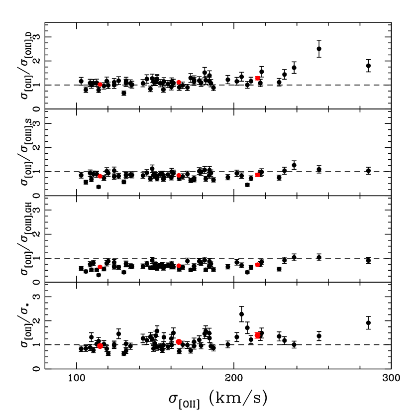
Figure 7: Ratio of [OII] width ($\sigma_{\rm[OII]}$) to [OIII] width as fitted with different methods ($\sigma_{\rm[OIII,D]}$, $\sigma_{\rm[OIII,S]}$, and $\sigma_{\rm[OIII,GH]}$) as well as to stellar-velocity dispersion ($\sigma_{\star}$; lower panel) as function of [OII] width ($\sigma_{\rm[OII]}$), for aperture spectra within the effective bulge radius. Red data points show average ratio within velocity bins 90-140 km s^-1, 140-190 km s^-1, and 240-290 km s^-1, respectively.

Table 5: Ratios of [OII] width to [OIII] width and stellar-velocity dispersion depending on fitting method and [OII] width. Col. (1): Extraction of spectra. Col. (2): Fitting method of [OIII] emission line. Col. (3): Mean and uncertainty (of the mean) of the resulting ratio of [OII] ($\sigma_{\rm[OII]}$) width to [OIII] width ($\sigma_{\rm[OIII]}$) and stellar-velocity dispersion ($\sigma_{\star}$) for all measurements. Col. (4): Same as Col. (3), but for [OII] width between 90-140 km s^-1. Col. (5): Same as Col. (3), but for [OII] width between 140-190 km s^-1. Col. (6): Same as Col. (3), but for [OII] width between 190-240 km s^-1.

Spectrum	[OIII] Fit	Mean Ratio	Mean Ratio	Mean Ratio	Mean Ratio
		Total	Bin 1	Bin 2	Bin 3
(1)	(2)	(3)	(4)	(5)	(6)
Effective radius (aperture)	Double Gaussian	1.17$\pm$0.04	1.02$\pm$0.03	1.12$\pm$0.03	1.28$\pm$0.07
	Single Gaussian	0.86$\pm$0.02	0.81$\pm$0.04	0.84$\pm$0.02	0.87$\pm$0.07
	Gauss-Hermite Polynomials	0.70$\pm$0.02	0.64$\pm$0.04	0.69$\pm$0.02	0.73$\pm$0.06
	Stellar-Velocity-Dispersion	1.15$\pm$0.04	0.95$\pm$0.05	1.13$\pm$0.04	1.4$\pm$0.1

4.4 Black Hole Mass - $\sigma_{\rm[OIII]}$ relation

We here compare the resulting $M_{\rm BH}$-$\sigma_{\rm[OIII]}$ relations with the “true” $M_{\rm BH}$-$\sigma_{\star}$ relation taken from Bennert et al. (2015). For comparison samples, we include quiescent galaxies (McConnell & Ma, 2013, 72 objects) and reverberation-mapped AGNs (Woo et al., 2015, 29 objects; adopting the same virial factor as for our sample; $\log f=0.71$). The results show that the total [OIII] emission line (as fitted by either a single Gaussian and even more extreme for Gauss-Hermite Polynomials) overestimates $\sigma_{\star}$ and the points scatter to the right of the relation (Fig. 8, bottom panels). However, when based on $\sigma_{\rm[OIII],D}$, our sample follows the same $M_{\rm BH}$-$\sigma_{\star}$ scaling relationship.

The systematic offset for the full [OIII] line width is significant, especially since it is of the same order as the expected evolutionary trend out to $z=1-2$ (e.g., Bennert et al., 2010, 2011b) and in the opposite direction. In other words, using the width of the full [OIII] line as surrogate for $\sigma_{\star}$ (e.g., by simply fitting a single Gaussian) in an attempt to study the evolution of the $M_{\rm BH}$-$\sigma_{\star}$ relation as done by e.g., Salviander et al. (2013) will suggest a null result, even though there actually is significant evolution.

Since our sample spans a small dynamical range in BH mass (6.7$<$$\log$$M_{\rm BH}$$<$8.2), and given the uncertainties of $M_{\rm BH}$ of 0.4 dex, we cannot determine the slope of the relationship independently. Instead, we fit the data by the linear relation

$$\log(M_{\rm BH}/M_{\odot})=\alpha+\beta\log(\sigma/200\,\rm km\,s^{-1})$$ (1)

taking into account uncertainties and keeping the value of $\beta$ fixed to the corresponding relationships of quiescent galaxies (5.64 for McConnell & Ma (2013) and 4.38 for Kormendy & Ho (2013)) or reverberation mapped AGNs (Woo et al., 2015, 3.97). The resulting zero point and scatter of the distribution are comparable to that of the quiescent galaxies. Table 6 summarizes the results for $\sigma_{\rm[OIII],D}$, including a comparison to a quiescent galaxies sample taken from Kormendy & Ho (2013, 51 objects; pseudo bulges and mergers excluded).

Note that the intrinsic scatter depends on the uncertainties of the measurements. For the quiescent galaxy sample, $M_{\rm BH}$ was derived from the kinematics of gas and/or stars within the gravitational sphere of influence of the BH; for the comparison AGN sample, $M_{\rm BH}$ was derived more directly through reverberation mapping. Thus, for those samples, the uncertainty on $M_{\rm BH}$ is significantly lower, on average 0.2dex and 0.15dex, respectively, compared to 0.4dex for the single-epoch method used for our sample. If, for example, for our $M_{\rm BH}$-$\sigma_{\star}$, we artificially assumed an uncertainty of $M_{\rm BH}$ of 0.17dex, the scatter would increase from 0.19 to 0.39 (for a fixed slope of 3.97), in other words, comparable to the 0.41 scatter of the reverberation-mapped AGN sample of Woo et al. (2015). Thus, the most direct comparison of scatter is between the scatter of the $M_{\rm BH}$-$\sigma_{\star}$ relation from Bennert et al. (2015) and that of the $M_{\rm BH}$-$\sigma_{\rm[OIII],D}$ relation here, since these are the identical samples with the same uncertainties in the $M_{\rm BH}$ measurements. Independent of assumed fixed slope, we find a smaller scatter in the $M_{\rm BH}$-$\sigma_{\rm[OIII],D}$ This is likely due to the fact that $\sigma_{\rm[OIII],D}$ covers a smaller dynamic range than $\sigma_{\star}$ (both within the effective bulge radius); however, since the scatter is within the range of uncertainties, we do not discuss this here further.

Table 6: Fits to the local $M_{\rm BH}$-$\sigma$ relation, $\log(M_{\rm BH}/M_{\odot})=\alpha+\beta\log(\sigma/200{\rm km\,s}^{-1})$. Col. (1): Sample and sample size in parenthesis. Col. (2): Mean and uncertainty on the best-fit intercept. Col. (3): Mean and uncertainty on the best-fit slope. Col. (4): Mean and uncertainty on the best-fit intrinsic scatter. Col. (4): References for fit. Note that the quoted literature uses FITEXY with a uniform prior on the intrinsic scatter, so our fits assume the same. The results from “this paper” are based on using $\sigma_{\rm[OIII],D}$ as surrogate for $\sigma_{\star}$. ^a Relation plotted as dashed lines in Fig. 8 and used as fiducial relation when calculating residuals.

Sample	$\alpha$	$\beta$	Scatter	Reference
(1)	(2)	(3)	(4)	(5)
Quiescent Galaxies (72)	8.32$\pm$0.05	5.64$\pm$0.32	0.38	McConnell & Ma 2013a
Quiescent Galaxies (51)	8.49$\pm$0.05	4.38$\pm$0.29	0.29	Kormendy & Ho 2013
Reverberation-mapped AGNs (29)	8.16$\pm$0.18	3.97$\pm$0.56	0.41$\pm$0.05	Woo et al. 2015
AGNs (66)	8.38$\pm$0.08	5.64 (fixed)	0.43$\pm$0.09	Bennert et al. 2015
AGNs (66)	8.20$\pm$0.06	4.38 (fixed)	0.25$\pm$0.10	Bennert et al. 2015
AGNs (66)	8.14$\pm$0.06	3.97 (fixed)	0.19$\pm$0.10	Bennert et al. 2015
AGNs (62)	8.41$\pm$0.07	5.64 (fixed)	0.25$\pm$0.11	this paper (based on $\sigma_{\rm[OIII],D}$)
AGNs (62)	8.23$\pm$0.06	4.38 (fixed)	0.14$\pm$0.09	this paper (based on $\sigma_{\rm[OIII],D}$)
AGNs (62)	8.16$\pm$0.06	3.97 (fixed)	0.12$\pm$0.08	this paper (based on $\sigma_{\rm[OIII],D}$)

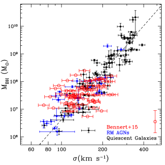
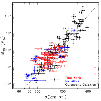
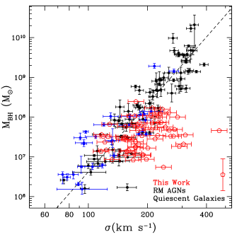
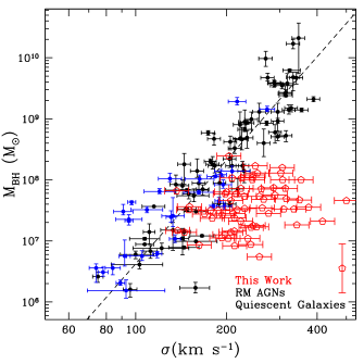
Figure 8: $M_{\rm BH}$-$\sigma_{\star}$ relation. Upper left panel: “True” $M_{\rm BH}$-$\sigma_{\star}$ relation for 65 objects presented in Bennert et al. (2015) (red open pentagons), reverberation-mapped AGNs (blue; Woo et al., 2015), and a sample of quiescent local galaxies (black; McConnell & Ma, 2013, with the black dashed line being their best fit). The error on the BH mass for our sample is 0.4 dex and shown as a separate point with error bar in the legend, to reduce confusion of data points. We assume a nominal uncertainty of the stellar-velocity dispersion of 0.04 dex. Upper right panel: The same as in the left panel, but for $\sigma_{\rm[OIII],D}$ (from aperture spectra within effective bulge radius; our sample only) instead of $\sigma_{\star}$ (as shown in the left panel, also derived within effective bulge radius). Lower panels: The same as in the upper right panel, but using the [OIII] width as fitted by a single Gaussian (left panel) and Gauss-Hermite polynomials (right panel), in both cases clearly overestimating the “true” $\sigma_{\star}$.

4.5 Comparison with FIRST

We searched the Very Large Array (VLA) Faint Images of the Radio Sky at Twenty-Centimeters (FIRST) catalog for radio detection. While our sample is radio quiet, out of the 62 objects in the M_BH-$\sigma_{\star}$ relation, 21 have been detected in FIRST, 37 objects have not been detected (FIRST detection limit $\sim$ 1mJy), and 4 objects are outside of the survey area. While for objects not detected in FIRST the ratio $\sigma_{\rm[OIII],D}$/$\sigma_{\star}$ is comparable to the overall average of our sample, i.e., close to 1, (1.05$\pm$0.02 for spatially-resolved data and 0.99$\pm$0.04 for aperture spectra within the bulge-effective radius, respectively), radio-detected objects have a larger width of [OIII], overestimating $\sigma_{\star}$ by 13% (the ratio is 1.13$\pm$0.03 for spatially-resolved data and 1.13$\pm$0.06 for effective-radius integrated spectra). When probing the broadening as a function of distance from the center, we see a trend that it is more pronounced towards the nucleus.

We color-code objects accordingly in the $M_{\rm BH}$-$\sigma$ relations (Figure 9). In the M_BH-$\sigma_{\star}$ relation, objects detected in radio vs. those undetected by FIRST do not form distinct populations. However, when using the width of the core [OIII] emission line (as traced by a double Gaussian, excluding the wing component), there is a trend of objects detected in FIRST having larger widths, especially those with lower $M_{\rm BH}$.

Our results show that the radio emission, even in these radio-quiet objects, has an effect on the [OIII] emission, broadening its dispersion, even for the core component. This effect has also been observed in radio-loud emission-line galaxies, where the [OIII] central component shows a strong trend of increasing line width with increasing central [OIII] peak shift (i.e., outflow velocity), likely due to strong jet-cloud interactions across the NLR (Komossa et al., 2018).

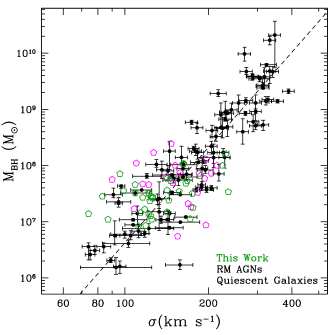
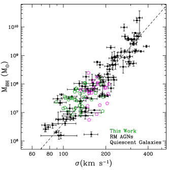
Figure 9: Same as in Figure 8, upper panels, but now distinguishing between objects detected in FIRST (magenta) and those with only upper limits (darkgreen); (literature samples shown in black). (No error bars shown to reduce confusion.) While there is no trend with $\sigma_{\star}$ (left panel), the radio does have a broadening effect on the [OIII] emission line (right panel), even when only considering the core of the line.

4.6 The potential and limitations of [OIII] width as a surrogate for $\sigma_{\star}$

Overall, the results presented above are in agreement with those of previous studies, concluding that the width of the narrow core of the [OIII] emission line can be used as a replacement for $\sigma_{\star}$, albeit with a large scatter (Nelson, 2000; Greene & Ho, 2005), when considering only the central [OIII] component (Komossa & Xu, 2007; Woo et al., 2016), when excluding sources with a blueshifted central [OIII] component since these objects show strong additional line broadening (Komossa et al., 2008), and when excluding objects with strong radio emission (Komossa et al., 2018). The resulting $M_{\rm BH}$-$\sigma_{\rm[OIII],D}$ correlation scatters around the known relation of quiescent galaxies.

However, when a direct comparison is made by plotting $\sigma_{\star}$ against $\sigma_{\rm[OIII],D}$, either from spatially-resolved data or integrated within an aperture of the effective bulge radius, there is no strong correlation between the two (Figure 10; Pearson linear correlation coefficients of 0.25 for spatially-resolved data and 0.41 for aperture data; same results for Spearman rank correlation coefficient; see also Liu et al. (2009)). This holds for both the radio-detected objects in the sample as well as the ones not detected in FIRST. Instead of a direct correlation between $\sigma_{\star}$ and $\sigma_{\rm[OIII],D}$, our data show that they cover the same range, and that their average and standard deviation are similar. Since we did not select on either quantity, but purely on H$\beta$ width, this indicates a physical connection and that they feel the same overall gravitational potential. As a consequence, the ratio of $\sigma_{\rm[OIII],D}$ to $\sigma_{\star}$ is close to one with a small deviation of the mean. And since we start out with a $M_{\rm BH}$-$\sigma_{\star}$ relation that follows that of quiescent galaxies and reverberation-mapped AGNs, this naturally results in $M_{\rm BH}$-$\sigma_{\rm[OIII],D}$ that scatter around the same relation. Given the large uncertainty in $M_{\rm BH}$ based on single-epoch masses (0.4 dex), a factor of 2 in $\sigma_{\rm[OIII],D}$/$\sigma_{\star}$ is still not that large.

At first sight, the absence of a strong correlation could be due to the fact that we cover a relatively small dynamic range in $M_{\rm BH}$, especially given the large uncertainty in $M_{\rm BH}$: the range covered is roughly twice the uncertainty. However, this is not true for measurements of $\sigma$: For $\sigma_{\star}$, our sample has a factor of $\sim$3 in dynamic range with a relatively small uncertainty (the range covered is roughly seven times the uncertainty). Thus, the fact that we do not find a close correlation is significant. While we cannot exclude that adding galaxies with larger $\sigma_{\star}$ would result in a trend, especially when considering mainly elliptical galaxies for which the underlying kinematic field is simpler, our sample consisting of AGNs hosted in mostly spiral galaxies (77% classified as Sa or later; Bennert et al., 2015) does not exhibit a significant correlation between $\sigma_{\star}$ and $\sigma_{\rm[OIII],D}$. 8 objects have been conservatively classified as having a pseudo-bulge (Bennert et al., 2015). These objects are not amongst any particular outliers in the $\sigma_{\star}$ and $\sigma_{\rm[OIII],D}$ plots. However, the sample size is small and the classification based on SDSS images for which a morphological classification is difficult, given the presence of the bright AGN point source. We will re-visit the question of pseudo-bulges with higher-resolution images (HST-GO-15215; PI: Bennert).

We consider the careful fitting of a double Gaussian, excluding wings and the use of the narrow core component for estimation of the [OIII] width, a robust approach; the $\sigma_{\star}$ measurements were taken with an equally great care (Harris et al., 2012). Our sample further has the advantage of high S/N spatially-resolved spectra, allowing a direct comparison of $\sigma_{\rm[OIII],D}$ and $\sigma_{\star}$ for the same object, using the same spectra and the same aperture. Thus, the reason for the scatter is likely a physical one. Generally speaking, both absorption and emission line profiles are a luminosity-weighted line-of-sight average, depending on the light distribution and the underlying kinematic field which can be different between gas and stars. Also, there may still be effects of outflows, inflows, and anisotropies not accounted for in the double Gaussian fitting of [OIII]. Finally, radiation pressure would only act on gas, not on stars. Our data do not allow to single out any of these as the main cause of the scatter.

Given the high quality of our kinematic data, both in terms of S/N of the spectra as well as the detailed fitting, the fact that we do not find a close correlation between $\sigma_{\rm[OIII],D}$ and $\sigma_{\star}$ strongly cautions against the use of $\sigma_{\rm[OIII],D}$ as a surrogate for $\sigma_{\star}$ on an individual basis, even though as an ensemble they trace the same gravitational potential.

Figure 10: Direct comparison between $\sigma_{\star}$ and $\sigma_{\rm[OIII],D}$. The dashed line indicates the one-to-one relation. The left panel shows the result from spatially-resolved data, the right panel from aperture data, integrated within the effective bulge radius.

5 Summary

We study the spatially-resolved [OIII]$\lambda$5007Å emission line profile of a sample of $\sim$80 local ($0.02\leq z\leq 0.1$) type-1 Seyfert galaxies. Stellar-velocity dispersion ($\sigma_{\star}$) derived from high-quality long-slit Keck spectra is used to probe whether the width of the [OIII] emission line, obtained by three different methods, is a valid substitute for $\sigma_{\star}$. Since the [OIII] emission line is known to often have broad wings from non-gravitational motion, such as outflow, infall or turbulence, we fit the line with a double Gaussian. For comparison, we include a single Gaussian fit, the simplest fit, and Gauss-Hermite polynomials which yield the best overall fit to the line. Our results can be summarized as follows.

1. In 66% of the spectra we find the presence of a blue wing, 22% of the spectra show a red wing, and in 12% of the cases, a broader central component is seen.

2. The width of the narrow core component of [OIII] from a double Gaussian fit, is, on average, the closest tracer of $\sigma_{\star}$ (mean ratio of 1.06$\pm$0.02 for spatially-resolved spectra and 1.02$\pm$0.04 for spectra within aperture of effective radius, respectively). However, the scatter is large, with individual objects off by up to a factor of 2.

3. Fitting [OIII] with a single Gaussian or Gauss-Hermite polynomials results in a width that is, on average, 50-100% larger than the stellar-velocity dispersion. This strongly cautions against the use of the full [OIII] width as a surrogate for $\sigma_{\star}$ in evolutionary studies, since the systematic offset will mimic a null-result.

4. We do not find trends of the $\sigma_{\rm[OIII]}/\sigma_{\star}$ ratio with distance from the center nor dependencies on other properties of the AGN (such as BH mass and $L_{5100}$) or the host galaxy (such as morphology and inclination).

5. Even though our sample consists of radio-quiet Seyfert galaxies, $\sim$30% have FIRST detections. The radio emission even effects the [OIII] core width, leading to $\sim$10% broader lines.

6. When considering the width of the narrow core component of [OIII], the resulting $M_{\rm BH}$-$\sigma_{\rm[OIII],D}$ relation scatters around the $M_{\rm BH}$-$\sigma_{\star}$ relations of quiescent galaxies and reverberation-mapped AGNs.

7. We compare the width of the doublet [OII]$\lambda\lambda$3726,3729ÅÅ, fitted by a double Gaussian, with those of [OIII] and $\sigma_{\star}$. While wings are less prominent in the low-ionization [OII] line, they are nevertheless present, especially for wider lines, but harder to fit given the blended nature of the line and the lower S/N. Thus, [OIII] is preferable over [OII].

8. A direct comparison between $\sigma_{\star}$ and $\sigma_{\rm{[OIII]}}$ shows that there is no correlation on an individual basis. Overall, gas and stars follow the same gravitational potential and thus have similar distributions in terms of range, average, and standard deviation. This results in an average ratio of $\sigma_{\rm[OIII],D}$ to $\sigma_{\star}$ close to one, with a small deviation of the mean, and an $M_{\rm BH}$-$\sigma_{\rm[OIII],D}$ relation that scatters around those of quiescent galaxies and reverberation-mapped AGNs.

9. The reason for the large scatter is likely a physical one. Line profiles are luminosity-weighted line-of-sight averages that depend on the light distribution and the underlying kinematic field which can be different between gas and stars. Moreover, effects of outflows, inflows, anisotropies and radiation pressure on the [OIII] profile not accounted for in the double Gaussian fitting can increase the scatter.

10. Given the large dynamic range covered in $\sigma_{\star}$ and the high quality of our kinematic data, our results are significant and caution against the use of [OIII] as a surrogate for $\sigma_{\star}$ on a case-by-case basis, even though as an ensemble they trace the same gravitational potential.

References

- Barrera-Ballesteros et al. (2015) Barrera-Ballesteros, J. K., et al. 2015, å, 582, A21
- Beifiori et al. (2012) Beifiori, A., Courteau, S., Corsini, E. M., & Zhu, Y. 2012, MNRAS, 419, 2497
- Bennert et al. (2010) Bennert, V. N., Treu, T., W. J.-H., Malkan, M. A., Le Bris, A., Auger, M. W., Gallagher, S., & Blandford, R. D. 2010, ApJ, 708, 1507
- Bennert et al. (2011a) Bennert, V. N., Auger, M. W., Treu, T., Woo, J.-H., & Malkan, M. A. 2011a, ApJ, 726, 59
- Bennert et al. (2011b) Bennert, V. N., Auger, M. W., Treu, T., Woo, J.-H., & Malkan, M. A. 2011b, ApJ, 742, 107
- Bennert et al. (2015) Bennert, V. N., Treu, T., Auger, M. W., et al. 2015, ApJ, 809, 20
- Bonning et al. (2005) Bonning, E. W., Shields, G. A., Salviander, S., & McLure, R. J. 2005, ApJ, 626, 89
- Boroson (2003) Boroson, T. A. 2003, ApJ, 585, 647
- Boroson & Green (1992) Boroson, T. A., & Green, R. F. 1992, ApJS, 80, 109
- De Robertis & Osterbrock (1984) De Robertis, M. M., & Osterbrock, D. E. 1984, ApJ, 286, 171
- van der Marel (1994) van der Marel, R. P. 1994, MNRAS, 270, 271
- Davis et al. (2011) Davis, T. A., et al., 2011, MNRAS, 417, 882
- Dasyra et al. (2008) Dasyra, K. M., Ho, L. C., Armus, L., Ogle, P., Helou, G., Peterson, B. M., Lutz, D., Netzer, H., & Sturm, E. 2008, ApJ, 674, L9
- Dasyra et al. (2011) Dasyra, K. M., Ho, L. C., Netzer, H., Combes, F., Trakhtenbrot, B., Sturm, E., Armus, L., & Elbaz, D., ApJ, 740, 94
- Greene & Ho (2005) Greene, J. E., & Ho, L. C. 2005, ApJ, 627, 721
- Grupe & Mathur (2004) Grupe, D., & Mathur, S. 2004, ApJ, 606, L41
- Harris et al. (2012) Harris, C. E., Bennert, V. N., Auger, M. W., et al. 2012, ApJS, 201, 29
- Heckman et al. (1981) Heckman, T. M., Miley, G. K., van Breugel, W. J. M., & Butcher, H. R. 1981, ApJ, 247, 403
- Ho (2009) Ho, L. C. 2009, ApJ, 699, 638
- Jin et al. (2016) Jin, Y., Chen, Y., Shi, Y. et al. 2016, MNRAS, 463, 913
- Kollatschny & Zetzl (2013) Kollatschny, W. & Zetzl, M, 2013, å, 549, 100
- Komossa & Xu (2007) Komossa, S., & Xu, D. 2007, ApJ, 667, 33
- Komossa et al. (2018) Komossa, S., Xu, D. W., & Wagner, A. Y. 2018, MNRAS, 477, 5115
- Komossa et al. (2008) Komossa, S., Xu, D. Zhou, H., Storchi-Bergmann, T., & Binette, L. 2008, ApJ, 680, 926
- Kormendy & Ho (2013) Kormendy, J., & Ho, L. C. 2013, ARAA, 51, 511
- Liu et al. (2009) Liu, X., Zakamska, N. L., Greene, J. E., Strauss, M. A., Krolik, J. H., & Heckman, T. M. 2009, ApJ, 702, 1098
- McConnell & Ma (2013) McConnell, N. J. & Ma, C.-P. 2013, ApJ, 764, 184
- McGill et al. (2008) McGill, K. L., Woo, J. H., Treu, T., & Malkan, M. A. 2008, ApJ, 673, 703
- Mullaney et al. (2013) Mullaney, J. R., Alexander, D. M., Fine, S., Goulding, A. D., Harrison, C. M., & Hickox, R. C. 2013, MNRAS, 433, 622
- Nelson (2000) Nelson, C. H. 2000, ApJ, 544, 91
- Nelson & Whittle (1996) Nelson, C. H., & Whittle, M. 1996, ApJ, 465, 96
- Netzer & Trakhtenbrot (2007) Netzer, H., & Trakhtenbrot, B. 2007, ApJ, 654, 754
- Park et al. (2015) Park, D., Woo, J. H., Bennert, V. N., et al. 2015, ApJ, 799, 164
- Rice et al. (2006) Rice, M., et al. 2006, ApJ, 636, 65
- Runco et al. (2016) Runco, J. N., Cosens, M., Bennert, V. N., Scott, B., Komossa, S., Malkan, M. A., Lazarova, M. S., Auger, M. W., Treu, T., & Park, D. 2016, ApJ, 821, 33
- Salviander et al. (2007) Salviander, S., Shields, G. A., Gebhardt, K. & Bonning E. W. 2007, ApJ, 662, 13
- Salviander et al. (2013) Salviander, S. & Shields, G. A. ApJ, 662, 13
- Salviander et al. (2015) Salviander, S., Shields, G. A., & Bonning, E. W. 2015, ApJ, 799, 173
- Sarzi et al. (2006) Sarzi, M., et al., 2006, MNRAS, 366, 1151
- Shankar et al. (2016) Shankar, F., Bernardi, M., Sheth, R. K., Ferrarese, L., Graham, A. W., Savorgnan, G., Allevato, V., Marconi, A., Läsker, R., & Lapi, A. 2016, MNRAS, 460, 3119
- Shields et al. (2003) Shields, G. A. et al. 2003, ApJ, 583, 124
- Terlevich et al. (1990) Terlevich, E., Diaz, A. I., & Terlevich, R. 1990, MNRAS, 242, 271
- Valdez et al. (2004) Valdez, F., Gupta, R., Rose, J. A., Singh, H. P., & Bell, D. J. 2004, ApJS, 152, 251
- van der Marel & Franx (1993) van der Marel, R. P. & Franx, M. 1993 ApJ, 407, 525
- Wang & Lu (2001) Wang, T. & Lu, Y. 2001, å, 377, 52
- Wilson & Heckman (1985) Wilson, A. S., & Heckman, T. M. 1985, in Astrophysics of Active Galaxies and Quasi-Stellar Objects, ed. J. S. Miller (Mill Valley: University Science Books), 39
- Whittle (1985) Whittle, M. 1985, MNRAS, 213, 1
- Whittle (1992) Whittle, M. 1992, ApJ, 387, 109
- Woo et al. (2006) Woo, J. H., Treu, T., Malkan, M. A., & Blanford, R. D. 2006 ApJ, 645, 900
- Woo et al. (2015) Woo, J.-H., Yoon, Y., Park, S., Park, D., & Kim, S. C. 2015, ApJ, 801, 1
- Woo et al. (2016) Woo, J.-H., Bae, H.-J., Son, D. & Karouzos, M. 2016, ApJ, 817, 108
- Woo et al. (2018) Woo, J.-H., Le, H. A. N., Karouzos, M., Park, D., Park, D., Malkan, M. A., Treu, T., & Bennert, V. N. 2018, ApJ, 859, 138