Synthetic Spectral Signatures from Isothermal Collapsing Gas and the Interpretation of Infall Profiles

Abstract

We revisit the interpretation of blue-excess molecular-line profiles from dense collapsing cores, considering recent numerical results suggesting that the prestellar stage of core collapse occurs from the outside-in, rather than inside-out. We thus perform synthetic molecular-line observations of simulated collapsing, spherically-symmetric, density fluctuations of low initial amplitude, embedded in a uniform, globally gravitationally unstable background, without a turbulent component. The collapsing core develops a flattened, Bonnor-Ebert-like density profile, but with an outside-in radial velocity profile, where the maximum infall speeds occur at large radii, where the density is already decreasing, with cloud-to-core accretion, and no hydrostatic outer envelope. Using the optically thick HCO⁺ $J=1-0$ and $3-2$ rotational transitions, we consider several “typical” beamwidths and use a simple line-fitting model to infer infall speeds from the synthetic profiles similarly to how it is done by standard line modeling. We find that the model-derived infall speeds are up to $3-4$ times smaller than the actual peak infall speeds, because the largest infall speeds are downweighted by the low density of the gas in which they occur, due to the outside-in nature of the actual radial infall speed profile. Also, using the isolated N₂H⁺ $J_{\rm F_{1}F}=1_{01}-0_{12}$ hyperfine component, we investigate the variation in the so-called asymmetry parameter, $\delta v\equiv(V_{\rm thick}-V_{\rm thin})/\Delta v_{\rm thin}$, during the collapse, finding good agreement with observed values. Finally, the HCO⁺ $J=3-2$ spectra exhibit extreme $T_{\rm b}$/$T_{\rm r}$–ratios similar to those observed in evolved cores, for the larger beamwidths late in the collapse. Our results suggest that standard dynamical infall reproduces several features from observations, but that low-mass core infall speeds are generally underestimated, often interpreted as being subsonic even when the actual speeds are supersonic, due to the incorrect assumption of an inside-out infall radial velocity profile with a static outer envelope.

1 Introduction

1.1 The molecular-cloud background of collapsing cores

The process by which dense molecular cloud (MC) cores collapse to form stars is still an unsettled issue. Under the old picture of magnetically-supported clouds with collapse mediated by ambipolar diffusion (e.g., Shu et al., 1987; Mouschovias, 1991), MCs were assumed to be Jeans unstable, but generally had magnetically subcritical mass-to-magnetic flux ratios, so that they were globally supported by the magnetic field against their self-gravity. Dense cores would grow quasistatically as ambipolar diffusion allowed local condensations of neutral material to gradually permeate through the magnetic field lines, until the local mass-to-flux ratio became supercritical, and dynamical collapse could proceed.

However, several issues with that picture emerged at the turn of the century (see Mac Low & Klessen, 2004, for a review), not the least of which is the realization that MCs are, in general, magnetically supercritical (Crutcher et al., 2010), and therefore not globally supported by the magnetic field. Instead, the current prevalent “gravoturbulent” view is that MCs are supersonically turbulent, and globally supported against collapse by virialized turbulent motions (e.g., Vázquez-Semadeni et al., 2003; Mac Low & Klessen, 2004), while simultaneously this turbulence induces small-scale density fluctuations in which the local Jeans mass may become smaller than the fluctuation’s own mass, and therefore the latter begins to undergo gravitational collapse (see, e.g., the reviews by Mac Low & Klessen, 2004; Ballesteros-Paredes et al., 2007; McKee & Ostriker, 2007).

Somewhat surprisingly, notions about dense MC cores that had originated in the magnetic-support scenario have migrated to the gravoturbulent one, despite it not being clear precisely how they would fit into that scenario. Chief amongst these is the notion that cores undergo a stage of quasistatic evolution, especially during their prestellar stage. During this stage, the cores are believed to be Jeans-stable, and confined by external pressure (e.g., Bertoldi & McKee, 1992; Lada et al., 2008). This notion has been reinforced by the frequent observation that cores exhibit Bonnor-Ebert-like (BE-like) column density profiles (e.g Alves et al., 2001), since BE spheres are known solutions of the hydrostatic Lane-Emden equation. Proposals have been made that, during this stage, the cores accrete material from their surroundings, until they become Jeans-unstable and begin to collapse dynamically (e.g., Simpson et al., 2011).

However, it is not clear how the cores could achieve a quasistatic configuration if they are produced by dynamic compressions in a supersonically turbulent medium, as the gravoturbulent scenario proposes, and several complications arise. First, a Jeans-stable, pressure-confined configuration requires the presence of a tenuous confining medium for the dense cores – i.e., at the sub-parsec scale—implying that MCs should be two-phase media even down to these scales. This is because equilibrium configurations in single-phase media are generally unstable, and therefore not expected to be realized in a supersonically turbulent medium (Vázquez-Semadeni et al., 2005). Second, it is not at all clear why a hydrostatic configuration would arise first, and then continue to accrete quasistatically from its surrounding medium if it was initially formed by a turbulent compression that was dynamic to begin with. In this case, evolving configurations are formed that accrete through shocks. Before the shock-confined structure becomes Jeans-unstable, it expands, and once it does become unstable, it begins to collapse (Gómez et al., 2007), and never undergoes a quasistatic stage. It is often suggested that perhaps the turbulent cascade feeds turbulence within the cores that supports them until it is dissipated, at which time they become unstable and collapse (e.g., Bergin & Tafalla, 2007; Keto et al., 2015). However, simulations of collapsing turbulent clumps never show an intermediate stable stage, after which the collapse would resume at the local scale. Instead, the cores form and either disperse or proceed directly to collapse (e.g., Vázquez-Semadeni et al., 1998, 2005, 2017; Robertson & Goldreich, 2012; Offner et al., 2014; Murray et al., 2017).

A possible resolution to these problems is offered by the recent proposal of global, hierarchical gravitational collapse of MCs (Burkert & Hartmann, 2004; Hartmann & Burkert, 2007; Vázquez-Semadeni et al., 2007; Vázquez-Semadeni et al., 2009; Heitsch & Hartmann, 2008; Naranjo-Romero et al., 2015, hereafter Paper I). In this scenario, MCs are born turbulent because of the combined action of several instabilities during their assembly stage (Koyama & Inutsuka, 2002; Heitsch et al., 2005; Vázquez-Semadeni et al., 2006), but are also strongly Jeans-unstable (i.e., containing many Jeans masses), because the gas entering them suffers a phase transition from the warm-diffuse atomic phase to the dense-cold phase, thereby increasing their density and decreasing their temperature by a factor of $\sim 10^{2}$, causing a reduction of their Jeans mass ($\propto\rho^{-1/2}T^{3/2}$) by a factor of $\sim 10^{4}$ (Gómez & Vázquez-Semadeni, 2014). Therefore, the clouds engage in global gravitational contraction. As they do, the average Jeans mass in the cloud decreases, because of the increasing mean density (at roughly constant temperature), and then the small-scale density fluctuations, induced by the turbulence, can undergo a collapse of their own when their mass surpasses the average Jeans mass in the cloud. This process then consists of collapses within collapses (Heitsch et al., 2008; Vázquez-Semadeni et al., 2009), and is essentially the same as Hoyle fragmentation (Hoyle, 1953), except that the density fluctuations are nonlinear, due to the moderate turbulence induced into the cloud during formation. The nonlinearity of the fluctuations and the multi-Jeans-mass nature of the clouds eliminates early concerns about this mechanism (Tohline, 1980).

In Paper I we presented a numerical simulation of the prestellar collapse of a local, near-Jeans-mass fluctuation embedded in a nearly uniform, multi-Jeans mass medium, with spherical symmetry. This simulation aimed at being an idealized model of the onset of collapse of a fluctuation located in the outskirts of a much larger-scale unstable object, so that the large-scale collapse center was located outside of the numerical box. The simulation was similar to the classic calculations of Larson (1969), except for the additional ingredient of being embedded in a uniform, strongly Jeans unstable background. Note that the initial fluctuation was very moderate, of only a 50% enhancement above the background level.

This simulation produced a number of interesting features. First, it developed a BE-like density profile (with a flat central region and a power-law envelope), but it was never in equilibrium, because the fluctuation only provided a focusing center to the collapsing tendency of the uniform background. So, even during the stages when the ratio of the central to the boundary density (with the boundary defined as the radius where the core merges into the background) was less than the critical value for BE sphere instability, the fluctuation was in the process of collapse. This naturally explains the growth of cores when they appear to be Jeans-stable and pressure confined. Second, the core developed an “outside-in” velocity profile (see also Whitworth & Summers, 1985; Gong & Ostriker, 2011), whereby the central parts of the core have a velocity that increases linearly with radius, and the outer parts have a uniform velocity, out to where the collapsing region extends. Third, the core, with its boundary defined as explained above, traces the locus of both low- and high-mass cores in a diagram of $M_{\rm c}/M_{\rm BE}$ versus $M_{\rm c}$, first proposed by Lada et al. (2008), where $M_{\rm c}$ is the core’s mass and $M_{\rm BE}$ is its BE mass, even in the region occupied by “stable” cores. This result suggested that both low- and high-mass cores are essentially Jeans-mass fluctuations undergoing collapse in a multi-Jeans mass medium.

1.2 Infall speed determination from molecular line profiles

However, one main caveat to this picture remained: that the simulated core developed supersonic infall speeds shortly before it forms a singularity (a protostar), in contradiction with the generally-accepted notion that low-mass starless cores, in particular, exhibit subsonic, not supersonic, infall speeds, as determined from their molecular-line emission (e.g., Lee et al., 2001). Indeed, moderately optically thick molecular line transitions of non-homologously collapsing cores are known to produce a self-reversed (i.e., with a self-absorption central dip) profile with a blue excess (e.g., Snell & Loren, 1977; Zhou, 1992; Evans, 1999) or, if the line is narrow, a single blue peak with a red shoulder. However, as dicussed by Evans (1999), blue-excess profiles can be caused by several other mechanisms (see also Leung & Brown, 1977), and so he advised that, to be a plausible candidate for collapse, a core must exhibit both (i) the self-reversed blue-skewed profile in a suitable optically-thick transition and (ii) a gaussian-like profile in an optically-thin line peaking at the self-absorption dip of (i). For (ii), the strength and skewness must peak at the central source. In this way, the two peaks of the blue-skewed profile should not be caused by clumps in an outflow.

To infer the infall speed of an observed core from a blue-skewed line profile, it is necessary to make an assumption on the form of the radial velocity profile in the core. One of the earliest assumptions made (e.g., Snell & Loren, 1977; Zhou et al., 1993) was that of an inside-out collapse, resulting from the collapse of an initially static singular isothermal sphere (SIS; Shu, 1977). However, this solution of the spherical, isothermal collapse has been deemed unrealistic (Whitworth et al., 1996) because the SIS is an unstable equilibrium, that is not expected to occur in general, let alone as a consequence of a dynamic turbulent compression. Therefore, other assumptions for the radial velocity profile have been made, including a simple two-layer model (e.g., Myers et al., 1996; Lee et al., 2001), and an initially unstable BE (or BE-like) sphere (e.g., Whitworth & Ward-Thompson, 2001; Keto et al., 2015).

Instead, the calculation presented in Paper I allowed the radial density and velocity profiles to develop self-consistently from the instant the core was a minor perturbation in the background flow. This core could collapse even when its amplitude was only 50% above the mean density because the entire simulation was gravitationally unstable, thus essentially only providing a focusing center for the collapse of the whole region.

As explained above, this setup allowed a natural definition of the instantaneous radial extent of the core, namely the radius at which the perturbation merged into the uniform background. This boundary definition is inspired by observations, since observed cores are usually either defined down to the noise level or to where they merge with the background (e.g., André et al., 2014). This kind of definition, however, does not imply that the cores actually end, or have a sharp density discontinuity at their operationally-defined boundaries. Instead, cores are known to be, in general, part of an extended continuum, which consists of their parent molecular clouds. With this definition, the numerical core grew both in mass and radius over time, accreting material from the surrounding cloud, and therefore does not coincide with any of the numerical model setups used previously (although see Mohammadpour & Stahler, 2013, for a related experiment), despite this being a more realistic situation for a dense core than, for example, a tenuous confining medium for the core (e.g., Ebert, 1955; Bonnor, 1956; Hunter, 1977; Mouschovias, 1976; Keto & Caselli, 2010; Keto et al., 2015).

Nevertheless, one remaining caveat of the simulation presented in Paper I was that the infall speeds developed by the model become supersonic during the latest stages of the prestellar evolution, in apparent contradiction with the observed subsonic speeds typically measured in low-mass cores (Lee et al., 2001). This apparent contradiction in fact led Mohammadpour & Stahler (2013) to conclude that a similar numerical experiment, with a fixed accretion rate from its environment, was not realistic.

In the present paper, we choose instead to investigate whether the apparently subsonic observed velocities may in fact be an artifact of an unrealistic assumption for the underlying core radial velocity profile. This is because in our core the collapse proceeds in an outside-in fashion, with the maximum infall speed occurring at the envelope of the core, not its center, as in the inside-out collapse of Shu (1977). Since line profiles are essentially density-weighted line-of-sight (LOS) velocity histograms modified by absorption, having the maximum speeds at radii where the density is decreasing suggests that these high infall speeds are down-weighted by the declining density in the envelope.

Various forms of a similar radial velocity profile, where the peak is outside the core center, already exist in the literature. Lee et al. (2007) found the contraction speed for L694-2 to be small at the envelope, rising to a maximum of 0.28 ${\rm km\ s}^{-1}$ at a distance of $\sim$ 0.08 pc from the center and decreasing inwards thereafter. Analogously, with a similar velocity profile, they found a peak infall speed of 0.2 ${\rm km\ s}^{-1}$ at 0.095 pc from the center for L1197. Such velocity profiles more satisfactorily match the broader linewidths observed in both cores from their single-dish HCN $J=1-0$ data.

One of the classic indicators of collapse is the presence of a blue-skewed line profile, which is defined as a bimodal profile in which the blue peak intensity ($T_{\rm b}$) exceeds the red peak intensity ($T_{\rm r}$), i.e. $T_{\rm b}/T_{\rm r}>1$. Numerous methods have been devised in the literature to interpret these profiles and derive infall velocities from them (e.g., Anglada et al., 1987, 1991; Zhou, 1992; Zhou et al., 1993; Myers et al., 1996; Evans, 1999; De Vries & Myers, 2005). For example, the simple two-layer analytical model of Myers et al. (1996) predicts that $T_{\rm b}/T_{\rm r}$ increases with increasing $v_{\rm in}$. This ratio appears extreme among a number of starless and protostellar cores. The low-mass starless core B133 displays a value of $3.14\pm 0.45$ (HCO⁺$J=3-2$, Gregersen & Evans, 2000), while a value of $3.40\pm 0.25$ is observed towards the high mass protostar associated with NGC 7538 (HCO⁺$J=1-0$, Sun & Gao, 2009). Such values in early collapsing cores are too large to be explained by current collapse theories (Gregersen & Evans, 2000). Mardones (1998) found the greatest $T_{\rm b}/T_{\rm r}$–ratios for a model in which the entire cloud is collapsing.

Furthermore, observations of line asymmetry in CS and HCO⁺ lines far from the core center combined with these extreme $T_{\rm b}/T_{\rm r}$–values strengthen the case for an uninhibited gravitational infall.

To investigate the relationship between the actual infall speeds and those inferred from the line profile using typical line-modeling techniques, we present, in this paper, synthetic spectral line observations of a numerical simulation of the collapse of a spherical core in the context of the global hierarchical gravitational collapse of a cloud; i.e., the collapsing core is embedded in a globally unstable background medium. To this end, we briefly discuss the numerical simulation, the bases for selecting the lines and a prescription for the synthetic spectra (§2). We then describe the various algorithms we apply to catergorize the infall signature (§3) and subsequently infer infall speeds from the blue-excess synthetic lines. Finally, we present the results of this work (§4), a discussion of these results in the context of existing observational literature (§5) and our conclusions (§6).

2 The Input Model

2.1 The numerical simulation

To produce synthetic spectra for a collapsing core, we consider a numerical simulation, presented in Paper I, of a collapsing spherically symmetric core inside a gravitationally unstable uniform background. As discussed in Paper I, this configuration aims to represent the onset of collapse of a density fluctuation, embedded in a large-scale collapse flow focussing on a distant point in space, once it becomes locally unstable. Longmore et al. (2014) have referred to this flow regime as a “conveyor belt” flow, and identified it as operating in the Central Molecular Zone of the Galaxy. Gómez & Vázquez-Semadeni (2014) have also observed this type of flow in simulations of cloud evolution where filaments form that feed a massive hub, and local collapses occur within the filaments.

Due to limitations of the spectral code used for the simulation, and the non-inclusion of sink particles, the collapse was followed only over the prestellar stages of its evolution. Nevertheless, this allows us to specifically investigate the generation of the initial conditions of star formation.

In the simulation, the gas was isothermal, and initially at rest, with a uniform density, $n=10^{4}\,{\rm cm}^{-3}$, and a kinetic temperature, $T_{\rm k}=11.4$ K, implying an isothermal sound speed of $c_{\rm s}=0.2\,{\rm km\ s}^{-1}$. At this density and temperature, the Jeans length was $L_{\rm J}\equiv(\pi c_{\rm s}^{2}/G\rho)^{1/2}\approx 0.22$ pc, where a mean particle weight $\mu=2.36$ has been assumed. The numerical box had a size $L_{\rm b}=\sqrt{10}\,L_{\rm J}\approx 0.71$ pc per side, implying that it had a total mass $M\approx 207\,M_{\odot}\approx 31.6\,M_{\rm J}$, where $M_{\rm J}$ is the Jeans mass. The resolution was $512$ cells per dimension, implying a cell size of $1.4\times 10^{-3}$ pc. For the generation of the synthetic spectra, we consider only the central half-length sub-box of the simulation, of volume $0.047\,{\rm pc}^{3}\,(=(0.71\,{\rm pc}/2)^{3}$), centered on the highest density volume pixel (voxel).

On top of the uniform density field, a gaussian fluctuation of amplitude 50% and standard deviation equal to $L_{\rm J}/2\,$ was added, so that the density at the fluctuation peak was $1.5\times 10^{4}\,{\rm cm}^{-3}$. The fluctuation contains slightly more than one Jeans mass at the mean simulation density, although it would be undetectable by any standard observation because of the low contrast with the background. The mass increase caused by the fluctuation is so small that the mean density in the simulation does not vary appreciably from the background value of $10^{4}\,{\rm cm}^{-3}$.

Because the entire numerical box is Jeans-unstable, gravitational collapse ensues, focused towards the perturbation (which acts as a seed). The simulation terminates immediately before a singularity is produced, at $t\approx 2.14t_{\rm ff}$, where $t_{\rm ff}=\sqrt{3\pi/32G\rho}\approx 0.33$ Myr is the free-fall time at the mean density. The actual collapse time is longer than the free-fall time because during the initial stages, the gravitational energy of the fluctuation is almost balanced by the internal pressure gradient, as the fluctuation contains only a little over one Jeans mass (Larson, 1969). As the collapse proceeds, gravity becomes increasingly dominant, and the collapse rate asymptotically approaches the free-fall rate.

As described in Paper I, during its prestellar evolution, the core develops a density structure that resembles a BE sphere, but with a finite infall speed over a range of radii, rather than being hydrostatic. The core has an inner region where the density is nearly uniform and the infall speed increases nearly linearly with radius, and an outer envelope, where the density approaches an $r^{-2}$ profile and the infall speed is roughly uniform, in agreement with the “Band 0” solution of Whitworth & Summers (1985). The transition between the inner flat-density region and the outer envelope occurs at a radius of the order of the Jeans length for the central density and temperature (Keto & Caselli, 2010).

However, the feature that distinguishes our simulation from other simulations in which the core is artificially truncated at some radius, is that, due to the presence of the uniform unstable background, the density of our core does not continue to self-similarly decrease as $r^{-2}$ at arbitrarily long distances, but rather eventually reaches the background value, at which point the core merges into the background, and the density remains flat beyond this radius. This merging radius constitutes the boundary of our core. As time progresses, the boundary moves outwards at a fraction of the sound speed. For example, as indicated in Table 2 of Paper I, when the core is defined as a 12.5% enhancement over the background density, its radius grows from 0.074 pc at $t=0$ to 0.19 pc at $t=0.72$ Myr, implying that the radius grows at a speed $\sim 0.16\,{\rm km\ s}^{-1}$, while the sound speed is $0.2\,{\rm km\ s}^{-1}$. We refer to this boundary as $R_{-\infty}(t)$, and corresponds to a rarefaction front which started to propagate when the fluctuation started to collapse, and so it is much larger than the standard position of the rarefaction front of the classical inside-out solution of Shu (1977), to which we refer as $R_{\rm Shu}$(t), which only starts to propagate at the time of the formation of the protostar; i.e., at the ending time of our simulation. We further discuss the implications of this behavior in §5.2.1.

Beyond $R_{-\infty}$, the infall speed decreases again, being zero at the simulation boundary. Although the precise value of zero velocity is an artifact of the periodic boundary condition, qualitatively the decreasing nature of the infall speed is observed to occur even in large-scale simulations where the local collapses are far removed from the boundaries (e.g., Gómez & Vázquez-Semadeni, 2014). This is due to the fact that, at long distances, the density tends to decrease even in the extended cloud, and so the large-scale collapse is non-homologous, with higher density inner regions infalling faster than outer, lower-density ones.

As already mentioned above, we refer to the collapse regime of our core as “outside-in”, since the maimum infall speeds occur at a finite radius from the center, of the order of the Jeans length of the central density (Whitworth & Summers, 1985; Keto & Caselli, 2010), and this radius of maximum velocity approaches the center at a speed that eventually becomes supersonic, but without developing a shock until the time of singularity formation.

The fact that the infalling motions extend beyond the radius at which the core merges into the background (Fig. 1(a); see also Mohammadpour & Stahler, 2013) implies the development of an accretion flow from the cloud onto the core, a feature that cannot happen in simulations of collapse where the core is artificially truncated at some finite radius, as is customary (e.g. Larson, 1969; Hunter, 1977; Foster & Chevalier, 1993; Keto et al., 2015). Although of course our simulation also has a finite size, it is significantly larger than the core’s initial radius, allowing for the development of the accretion from the cloud onto the core.

As the collapse progresses, the maximum infall speed along the radial dimension–the nearly uniform speed in the envelope–increases with time. We denote it by $v_{\rm max}(t)$. This maximum infall speed becomes transonic at $1.6t_{\rm ff}$ (see Table 1). By the end of the simulation, the maximum infall speed has reached $\sim 3c_{\rm s}$, as is common in this kind of numerical simulation (e.g., Larson, 1969).

A number of snapshots during the prestellar evolution are investigated. Snapshot 49 was arbitrarily chosen as our earliest point along the evolutionary track of the collapsing core because at this time the density contrast between the core’s maximum and the background is roughly a factor of 3. Note that at the final snapshot, number 65, the contrast is $\sim 2000$ (see fig. 1(b)).

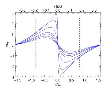
(a) Linear-linear radial velocity profile

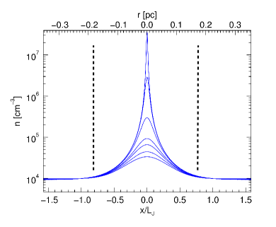
(b) Log-linear radial density profile

Figure 1: Radial profiles for (a) velocity and (b) density corresponding to the seven snapshots $49-65$ (inclusive) from Table 1. The dashed vertical lines in each panel demark the portion of the box considered in the radiative transfer analysis along each dimension (see §2.1). The log-linear form of (b) is necessary due to the marked increase in density between snapshots 64 and 65 prior to singularity formation. The two panels taken together, along the radial dimension, highlight the downweighting of higher velocity gas at the intermediate snapshots of Table 1 due to its location in the relatively lower density envelope.

Table 1: Physical Parameters of Analysed Snapshots

No.	$t_{\rm evol}^{a}$		$v_{\rm max}(t)^{b}$		$\Delta$xc
	(Myr)	($\times t_{\rm ff}$)	($\times c_{\rm s}$)	(${\rm km\ s}^{-1}$)	(pc)
49	0.54122	1.4489	0.6668	0.1333	0.1051
52	0.57340	1.5453	0.8087	0.1616	0.0982
55	0.60688	1.6465	1.0005	0.1999	0.0899
57	0.62583	1.7095	1.1590	0.2316	0.0830
61	0.67301	2.0065	1.6327	0.3263	0.0622
64	0.70598	2.1048	2.3093	0.4165	0.0346
65	0.71702	2.1377	2.8218	0.5639	0.0152

• ^aTime elaspsed since the beginning of the simulation, specified in terms of the free-fall time ($t_{\rm ff}$, see text) and in mega-years (Myr).

• ^bMaximum infalling speed at each snapshot, specified in terms of the sound speed ($c_{\rm s}$, see text) and in ${\rm km\ s}^{-1}$.

• ^cDistance in parsecs (pc) of gas at velocity of $v_{\rm max}(t)$ from the simulation box center at each snapshot.

2.2 Synthetic observations

We perform our synthetic observations using the accelerated (or approximate) lambda iteration (Rybicki & Hummer, 1991) radiative transfer code MOLLIE (Keto et al., 2004; Keto & Rybicki, 2010), which solves multi-level non-LTE radiative transfer problems ensuring rapid convergence of the radiation field and level populations. Assuming an initial input continuum radiation field and LTE population, the code calculates the new total radiation field and LTE populations. It then iterates until a specified convergence criterion is achieved. At each radial point the code generates (i) the level populations and (ii) the line source function. We use a fairly stringent convergence criterion $\Delta n_{i}/n_{i}\leq 10^{\rm-4}$, where $\Delta n_{i}$ represents the change in the converged level population, $n_{i}$, between the $(i-1)^{\rm th}$ and $i^{\rm th}$ iterations. The cosmic microwave background is the assumed initial radiation field in the radiative transfer calculations.

The emergent intensity distributions are then convolved with an appropriate synthetic telescope beam, so that the resulting spectra are comparable to observed line profiles from a given source observed with a specific telescope configuration. We assume that the telescope beam can be approximated by a Gaussian function, with a characteristic half-power beam width (HPBW). In typical observations of low-mass star-forming regions, the angular resolution (or beamwidth) of a single dish mm/sub-mm telescope is comparable to the angular size of nearby cores (e.g. Taurus- Auriga or Perseus MC cores). For this work, we consider beamwidths that are smaller than the simulated core dimension (up to $\sim 20\%$ of the core size).

2.3 Considerations for the synthetic spectral data

To produce synthetic spectral line data for our core, we first need to choose suitable optically thin and moderately optically thick lines. For the latter, we choose to focus on transitions that have sufficiently high critical densities but that are excited throughout the core gas. HCO⁺ is more opaque than either CS or H₂CO and so its rotational transitions are better suited to revealing infall during the later stages when less material remains in the envelope (Gregersen et al., 2000). The dipole moment of CS is 2.0 D, where D stands for $debyes$, while that of HCO⁺ is 3.3 D implying greater sensitivity to the dynamics of the central core region.

HCO⁺ transitions are optically thick at the densities typical of molecular cores ($10^{3}-10^{5}$ cm^-3) and so are useful for our simulated snapshots where the background density is 10⁴ cm^-3. HCO⁺ lines produce deeper self-absorptions than CS lines of similar frequency, not solely because of the relatively higher depletion of CS at higher densities towards the core centre, but because HCO⁺ predominates further out than CS and is therefore better able to trace the higher velocity component of the infalling gas. A noticeable feature in observational data is that HCO⁺ lines exhibit higher $T_{\rm b}$/$T_{\rm r}$–ratios than CS lines of similar frequency. Sun & Gao (2009) found, in their massive protostellar core survey, that, on average, $T_{\rm b}/T_{\rm r}\sim 2.2$ for HCO⁺ $J=1-0$ and $\sim 1.4$ for CS $J=2-1$, each with similar frequency. This disparity is due to the excitation conditions required for each transition and so each traces different spatial components of the core gas along the LOS. For HCO⁺, we consider a constant relative abundance of $3\times 10^{-9}$ (to H₂).

For the thin tracer, we choose N₂H⁺. This is a linear high-density tracing species containing seven hyperfine components in its lower $J=1-0$ rotational transition. Within this structure, the relatively isolated hyperfine component, $J_{\rm F_{1}F}=1_{01}-0_{12}$, maintains a near gaussian shape throughout the evolution of the simulated core. For N₂H⁺, we assume an abundance of 3$\times$10^-10 relative to H₂.

The ionized rotational collisional rate coefficients for collisions with $\rm H_{\rm 2}$ from Flower (1999) were used for the transitions of each of these species (see Table 2). Since HCO⁺ and N₂H⁺ have identical molecular masses, this approximation is roughly warranted. The modeled abundances for all considered transitions are typical of both low mass dark clouds and intermediate mass core conditions (Hogerheijde et al., 1997; Kirk et al., 2007).

Since the infall velocities at each step along the core’s evolution are comparable between adjacent snapshots (see Table 1) and the cloud is well radiatively coupled, the simple Sobolev large velocity gradient (LVG) radiative transfer approximation is not applicable (Leung & Brown, 1977). Additionally, as microturbulent radiative transfer codes artificially add an extra turbulent contribution to the velocity profile throughout the gas, hence creating broader line profiles (such as those applied by Zhou, 1992), we will not consider the microturbulent appoximation here (Masunaga & Inutsuka, 2000). A radiative transfer code that is capable of accounting for changes in physical parameters at the smallest scales, that is, non-LTE conditions, is more suitable.

Table 2: Modeled Molecular Transitions

Tracer†	$\nu$ (GHz)	$n_{\rm cr}^{*}$ (cm-3)
HCO+
$J=1-0$	89.18852	1.815$\times$105
$J=3-2$	267.55762	3.973$\times$106
N2H+
$J=1-0$	93.17370	1.549$\times$105
$J_{\rm F_{1}F}=1_{01}-0_{12}$	93.17625‡	1.549$\times$105

• ^∗Critical densities ($n_{\rm cr}=\nicefrac{{A_{\rm ul}}}{{\sum_{\rm u}q_{\rm ul}}}$) determined from the Leiden Atomic and Molecular Database (LAMDA).

• ^†Each tracer has a molecular mass of 29 amu (1 amu = $1.660538\times 10^{\rm-27}$ kg) resulting in an identical thermal velocity dispersion, $\sigma_{\rm th}=0.0572\,{\rm km\ s}^{-1}$.

• ^‡ The frequency of 93.17625 GHz actually corresponds to the location of three degenerate hyperfine lines: $J_{\rm F_{1}F}=1_{01}-0_{10}$, $1_{01}-0_{11}$, and $1_{01}-0_{12}$. The quantum number labelling of this line is routinely assigned to the latter on account of its higher relative intensity in the structure.

(a) Synthetic spectral positions for snapshot 52

(b) Synthetic spectral positions for snapshot 61

Figure 2: Synthetic line spectra for (a) snapshot 52 (top row) and (b) snapshot 61 (bottom row) at radial offsets $d$ (given in pc above each panel) from the core center. Each panel displays the HCO⁺ $J=3-2$ transition (solid line), the $\rm N_{\rm 2}H^{+}$ $J_{\rm F_{1}F}=1_{01}-0_{12}$ optically thin hyperfine component (dash-dotted line) and the best-fit Hill5 analytical model to the HCO⁺ transition (dotted line) corresponding to the lowest $NRMSD$-value. The beamwidth, $\theta_{\rm b}$, is 0.03 pc for both spectral strips. The upper right-hand corner of each panel displays the Hill5 derived infall velocity, $v_{\rm in}^{Hill5}$, the velocity dispersion of the $\rm N_{\rm 2}H^{+}$ hyperfine line, $\sigma$, and the $NRMSD$-value (see §3.2.1).

The resulting spectra from the radiative transfer runs are Hanning-smoothed, which results in the number of channels being halved. We initially tried a channel spacing of $0.01\,{\rm km\ s}^{-1}$ for accurate infall velocity determinations. The N₂H⁺$J=1-0$ transition with its quadrupolar hyperfine structure contained many more lines meaning a larger spread in velocity. A coarser velocity resolution of $0.02\,{\rm km\ s}^{-1}$ was therefore favored.

We create synthetic spectra for HCO⁺ rotational transitions. In particular, we focus on two rotational transitions: $J=1-0$ & $J=3-2$. Higher rotational transitions are particularly useful in investigating the velocity distribution in pre-stellar cores on account of their higher critical densities ($n_{\rm cr}$, see Table 2) than lower transitions of the same species since $n_{\rm cr}\propto\nu^{3}\mu^{2}$.

Three synthetic beamwidths, $\theta_{\rm b}$, are considered for the synthetic spectra created in this work (in parsecs): 0.015, 0.03 and 0.06 pc, respectively. These correspond to 22^′′, 44^′′ and 88^′′ at the distance of the Taurus-Auriga molecular complex ($\sim 140$ pc). The implemented beamwidths in parsecs are independent of the perceived distance of the simulated core. This is particularly useful in the comparison of our findings with observational data.

Example strips of line profiles for snapshots 52 and 61 are displayed in fig. 2 respectively at several radial positions on the core of constant separation as projected on a virtual “plane of the sky”.

3 Common spectral-line interpretation tools

Observed line profiles are usually interpreted in terms of various models of varying complexity, that focus on various features of the profile to extract information about the infall regime. In this section we review some of these techniques, so to later apply them to our synthetic profiles, and thus see what would normally be inferred from them. Thus, we can determine whether our numerical model and the synthetic line profiles obtained from it using MOLLIE are consistent with typical observed profiles, and how the standard interpretations compare with the actual physical conditions in our core.

3.1 Asymmetry Parameter: $\delta v$-Analysis

A first infall diagnostic for observed line profiles is the so-called asymmetry parameter ($\delta v$, Mardones et al., 1997):

$$\delta v=\frac{V_{\rm thick}-V_{\rm thin}}{\Delta v_{\rm thin}},$$ (1)

where $V_{\rm thick}$ represents the peak velocity of the optically thick line (in our case, each of the HCO⁺ $J=1-0$ and $3-2$ rotational lines). Likewise, $V_{\rm thin}$ represents the peak velocity of the optically thin line, and $\Delta v_{\rm thin}$ is its FWHM. A value $|\delta v|\geqslant 0.25$ indicates a strongly asymmetric line profile. Negative values imply blue-skewed and positive values imply red-skewed lines, respectively.

The synthetic lines from the simulated core allow us to compute $\delta v$ at each of the various evolutionary stages listed in Table 1, which can be directly compared to the values of this parameter observed in real prestellar cores. Using class (Buisson et al., 1994), we applied a global hyperfine fit to the N₂H⁺ $J=1-0$ hyperfine components (see Table 2 of Pagani et al., 2009, for degenerate and individual hyperfine lines in this transition) for all analysed synthetic spectral positions. By doing this, we were able to derive, explicitly, both $\Delta v_{\rm thin}$ and $V_{\rm thin}$ for use in eq. (1).

The quantity $\Delta v_{\rm thin}$ is the FWHM of each of the N₂H⁺ $J=1-0$ hyperfine components (assumed constant) in each class fit and $V_{\rm thin}$ is the relative shift in the peak velocity of the N₂H⁺ $J=1-0$ transition, assumed to represent the systematic motion of the cloud as a whole. This relative shift is brought about by the infalling motions in our simulated core, but must be determined with high precision so to obtain an accurate value for $\delta v$ from eq. (1). By using high-accuracy laboratory frequencies for all hyperfine components (Caselli et al., 1995) and determining their relative shifts with respect to the N₂H⁺ $J=1-0$ rotational transition frequency, we were able to compute their corresponding rest velocity shifts relative to the central “unshifted” rotational line (at 0 km s^-1). From the synthetic N₂H⁺ $J=1-0$ data, we were then able to determine the relative shifts of the individual hyperfine components from their rest relative velocities. Taking the average of these relative shifts allowed a more accurate determination of $V_{\rm thin}$.

The results from our $\delta v$–analysis are presented in figs. 3 and 4, for $J=1-0$ and $J=3-2$, respectively. The colored plots in each panel of these figures reflect a different value for $\theta_{\rm b}$ at which $\delta v$ was computed. We include a number of LOSs, of fixed separation (from the center), towards the core, for snapshots 49-65 (inclusive) from Table 1.

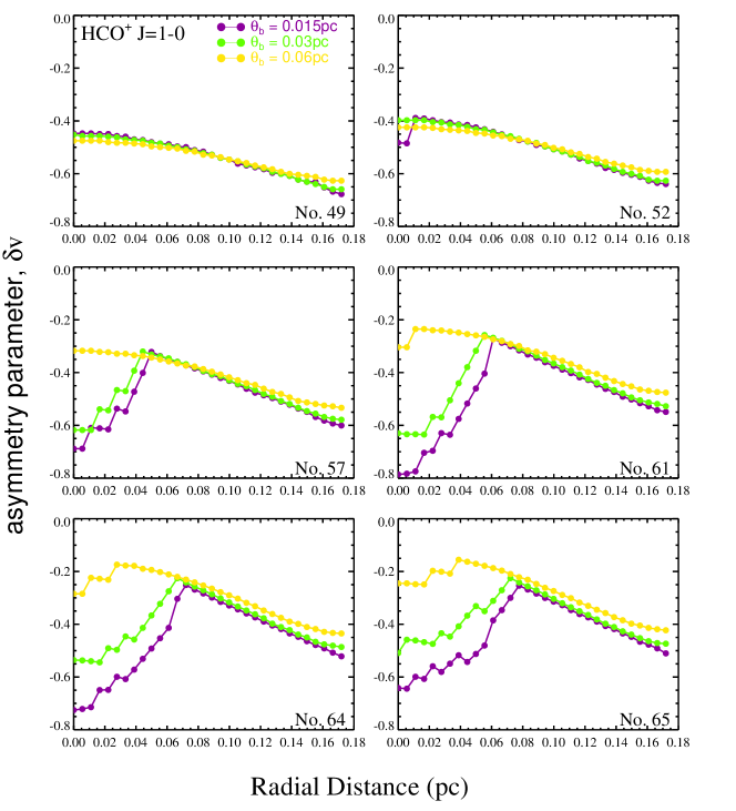
Figure 3: Radial dependence of the asymmetry parameter, $\delta v$, for the $J=1-0$ rotational transition. We include six snapshots in ascending order approaching the end of the simulation. This transition is affected by saturation, especially where $\theta_{\rm b}=0.015$ pc ($purple$) and 0.03 pc ($light~{}green$). For narrow beams, higher density gas becomes saturated leading to a wider separation of the peaks and hence larger values of $\left|\delta v\right|$. The extent of this saturation diminishes for $\theta_{\rm b}=0.06$ pc ($yellow$), where the derived values of $\left|\delta v\right|$ even out across the synthetic spectral map resulting in snapshot $\delta v$-curves resembling those for the HCO⁺ $J=3-2$ transition (compare with fig. 4).

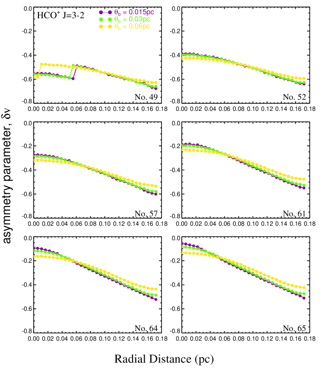
Figure 4: Radial dependence of the asymmetry parameter, $\delta v$, for the $J=3-2$ rotational transition. We include six snapshots in ascending order approaching the end of the simulation. The $\delta v$–values for this transitions are not overly affected by saturation and so one can infer the true radial variation of $\delta v$ and how that depends separately on both $\theta_{\rm b}$ (0.015 pc ($purple$), 0.03 pc ($light~{}green$) and 0.06 pc ($yellow$)) and the evolution of the core.

3.2 Hybrid Hill5 Analysis

The general solution to the equation of transfer, assuming the optical depth, $\tau$, increases away from the observer, is:

$$\Delta T_{\rm B}=T_{\rm i}e^{-\tau_{\rm 0}}+\int_{0}^{\tau_{\rm 0}}J(T_{\rm ex})e^{-\tau}d\tau$$ (2)

where $T_{\rm ex}$ is the excitation temperature of a region and varies over the optical depth interval, (0, $\tau_{0}$), and $T_{\rm i}$ is the incident specific intensity of radiation on that region at $\tau_{\rm 0}$, expressed in Kelvin. The Planck temperature, $J(T)=(h\nu/k)/(\exp(h\nu/kT)-1)$ is also in Kelvin.

A number of simplifying assumptions on the nature of $J(T)$ exist whereby the right-hand side of eq. (2) can be expressed exactly. The two-layer model (Myers et al., 1996) applies to an LOS in which two regions of differing $T_{\rm ex}$ move towards one another with the near region having a lower $T_{\rm ex}$ ($T_{\rm f}$) than the far region ($T_{\rm r}$). A constant $T_{\rm ex}$ is assumed along the LOS in this model. Lee et al. (2001) used such a model to derive typical infall velocities of $\sim 0.1\,{\rm km\ s}^{-1}$ for their starless core sample, comparable to the mean LOS linewidth, $\sigma_{\rm los}$, in this sample.

If $J$ in eq. (2) is defined as a linear function of $\tau$ (for all $\nu$) so that

$$J(\tau)=J_{\rm 1}+[(J_{\rm 2}-J_{\rm 1})/\tau_{\rm 0}]\times\tau,$$ (3)

(De Vries & Myers, 2005, hereafter DM05), where $J_{\rm 1}$ and $J_{\rm 2}$ are constants, the eq. (2) can be simplified as:

$$\Delta T_{\rm B}=T_{\rm i}e^{-\tau_{\rm 0}}+(J_{\rm 2}-J_{\rm 1})\times\frac{1-e^{-\tau_{\rm 0}}}{\tau_{\rm 0}}+J_{\rm 1}-J_{\rm 2}e^{-\tau_{\rm 0}}$$ (4)

where $\tau$ is a function of the Doppler velocity. DM05 defined their $Hill$ model using eqs. (3) and (4). This model includes a core with a peak $T_{\rm ex}=T_{\rm P}$ at the center (i.e. the maximum value of $J(\tau)$ in eq. (3)), and $T_{\rm ex}=T_{\rm 0}$ at both the near and far edges of the core (i.e. the minimum value of $J(\tau)$ for small $\tau$ in eq. (3)). Since this model requires that $J(\tau)$ depends linearly on $\tau$ between these extrema, the excitation profile (i.e. $J(\tau)$) forms a “hill”-profile (see fig. 1(b) of DM05).

The evolution of the two-layer model of Myers et al. (1996) to the Hill model of DM05 naturally occurred with our understanding that infall velocities are not simply determined from the separation of peaks in self-reversed line spectra. Since, although the velocity profile is identical in the two models, the provision of an inwardly-increasing $T_{\rm ex}$-profile in the latter enables the dependence of the infall motion on the extent of the blue-red asymmetry, i.e. the $T_{\rm b}/T_{\rm r}$–ratio, to be accounted for. It is on this basis that the Hill models are more effective than the two-layer models at matching self-absorbed excitation profiles observed in starless cores.

To solve the equation of radiative transfer, the Hill $T_{\rm ex}$–profile is split into two regions along the LOS: the first in the front part of the cloud, where $T_{\rm ex}$ increases along the LOS with optical depth $\tau_{\rm f}$ and the second in the rear part, where $T_{\rm ex}$ goes down along the LOS with optical depth $\tau_{\rm r}$, assuming a velocity dispersion of $\sigma$ in the entire cloud. The equation of transfer is then solved by integrating along the LOS through each of the two regions to derive the brightness temperature $\Delta T_{\rm B}(v)$, as a function of velocity.

The eight core parameters derived from the Hill model fit to the line profile are $\tau_{\rm c}$ (the line center optical depth of the core), $\sigma$, $T_{0}$, $T_{\rm P}$, $v_{\rm lsr}$ (the core systematic velocity), $v_{\rm in}$, $v_{\rm E}$ and $\tau_{\rm E}$ (the respective optical depth and velocity of an (optional) external envelope, where $T_{\rm ex}=T_{0}$). The Hill5 is a variant of the Hill model where $T_{\rm 0}$ is set to $T_{\rm b}$, the cosmic microwave background, with $v_{\rm E}=0$ and $\tau_{\rm E}=0$. According to DM05, beam smoothing does not adversely affect the accuracy of infall speeds obtained from this model.

We adopted a version of the Hill5 model, $Hill5hybrid$, that utilizes a hybrid minimization algorithm consisting of the differential evolution (DE) algorithm of Storn & Price (1997) that initially separates the local minima from the global minimum, for the combination of free parameters (discussed above) followed by Nelder-Mead simplex minimization (Nelder & Mead, 1965) to optimize the fit (DM05).

DE is an evolutionary algorithm that starts with a population of randomly generated parameters. This parameter set is randomly modified during each iteration until the global optimum solution is found. As the population evolves at each iteration, it is referred to as a generation.

The Hill5 routine takes six arguments. These are:

• rotational frequency in GHz (from Table 2)

• $v_{\rm min}$: the furthest leftward non-zero velocity value

• $v_{\rm max}$: the furthest rightward non-zero velocity value

• population in generation: the number of solutions to calculate each generation of the DE (used 300)

• generations per check: the number of generations to run before checking for convergence in the DE (used 300)

• checks to convergence: the number of checks to make before deciding the DE algorithm has converged (used 5)

Applying the model using the suggested parameters from DM05, the example fit in fig. 5, to a synthetic HCO⁺ $J=3-2$ spectrum (for snapshot 61 at $\theta_{\rm b}=0.06$ pc), is derived. A detailed analysis of $v_{\rm in}$ towards the simulated core at a selection of the times listed in Table 1 is given in §4.2.2 and displayed in figs. 6 and 7. Unlike in fig. 5, this analysis excludes fit values for $\tau_{\rm c}$, $T_{\rm P}$ etc., since we only invoked the Hill5 model to determine the value of $v_{\rm in}$ for each synthetic spectral position during the core’s evolution. In this way, the Hill5 model is used to exemplify the infall speed that known models would infer from the line spectra produced in this work. We do note, however, that $\tau_{\rm c}$ and $T_{\rm P}$ increase steadily with the density of the core gas, as expected.

Myers et al. (1996) determined an analytical expression for $v_{\rm in}$ from self-absorbed optically thick lines in terms of observable line parameters. Assuming $v_{\rm in}\ll\sigma(2\ln\tau_{0})^{\nicefrac{{1}}{{2}}}$, where $\sigma$ is the velocity dispersion of a concurrent optically thin line and $\tau_{0}$ is the line optical depth, they found (equation 9 in Myers et al., 1996):

$$v_{\rm in}^{an}\approx\frac{\sigma^{2}}{v_{\rm red}-v_{\rm blue}}\ln{\biggl{[}\frac{1+eT_{\rm BD}/T_{\rm D}}{1+eT_{\rm RD}/T_{\rm D}}\biggr{]}}.$$ (5)

where $T_{\rm D}$ is the height of the self-absorption dip, $T_{\rm BD}$ ($T_{\rm RD}$) is the height of the blue (red) peak above the dip, and $v_{\rm blue}$ ($v_{\rm red}$) represents the position of the blue (red) peak.

Tests, based on analytical models, for eq. (5) find that the analytically-derived value differs from the actual modeled $v_{\rm in}$ by up to 20% (Myers et al., 1996). Similarly, we determined the difference between the Hill5-derived value ($v_{\rm in}^{Hill5}$) and the corresponding analytical value ($v_{\rm in}^{an}$), from eq. (5), at various positions from the core’s center at the different snapshots in Table 1. For no position does the difference exceed 20-25%, with saturated positions at the latest snapshots falling into the higher end of this range. As an example, by applying eq. (5) to the spectrum in fig. 5, we find $v_{\rm in}^{an}=0.095$ km s^-1. From fig. 5, $v_{\rm in}^{Hill5}=0.116$ km s^-1, a 22% difference from $v_{\rm in}^{an}$. This result is in excellent agreement with the tests conducted by Myers et al. (1996) given that those tests restricted the infall velocity to values smaller than the velocity dispersion.

We should note that, from our analysis, eq. (5) is only suitable for use with centrally-located, strongly emitting asymmetric line profiles in the latest stages of collapse that precede star formation. It fails to adequately match the infall velocity for positions widely separated from the core center and spectra associated with earlier stages of the collapse, i.e. spectra with low $T_{\rm b}/T_{\rm r}$–ratios.

Figure 5: Synthetic spectrum for the HCO⁺ $J=3-2$ transition at a beamwidth, $\theta_{\rm b}=0.06$ pc, at the core center for snapshot 61 (see Table 1). Overplotted (dotted-line) is the Hill5 best-fit model to the synthetic data. Best-fit parameters are displayed (see text) together with the $NRMSD$-value of the fit (see §3.2.1).

3.2.1 Goodness-Of-Fit

To estimate the accuracy between the values predicted by the fit and the physically observed values for the core, we use the root mean square deviation ($RMSD$), defined as the square root of the mean squared error:

$$RMSD=\sqrt{\frac{\sum_{n}^{i=1}(y_{\rm o,i}-y_{\rm m,i})^{2}}{n}},$$ (6)

where, for this work, $y_{\rm m,i}$ is the $i$th estimated (or modeled) data point and $y_{\rm o,i}$ is the corresponding synthetic spectral data point, and the sum runs over the velocity channels i.

A comparative measure of the accuracy of each spectral fit contained in this work is the normalized $RMSD$, or $NRMSD$, calculated by dividing the $RMSD$ by the range of the synthetic data values in each Hill5 model fit:

$$NRMSD=\frac{RMSD}{y_{\rm o,max}-y_{\rm o,min}}$$ (7)

which we report as a percentage. Eq. (7) gives a suitable relative, scale-invariant measure (Hyndman & Koehler, 2006) that can be used to contrast the goodness-of-fit of the Hill5 model fits amongst all modeled spectral positions at each of the studied snapshots in Table 1. Relatively large $NRMSD$–values ($\gtrsim 10$%) indicate poor model fits where the underlying synthetic spectral data are either too saturated (e.g. $J=1-0$ data for snapshots later than 61) or where the self-absorption dip (see fig. 5 e.g., compare respective spectra in panels (a) and (b) from fig. 2) is too shallow (see §5.1 for further discussion).

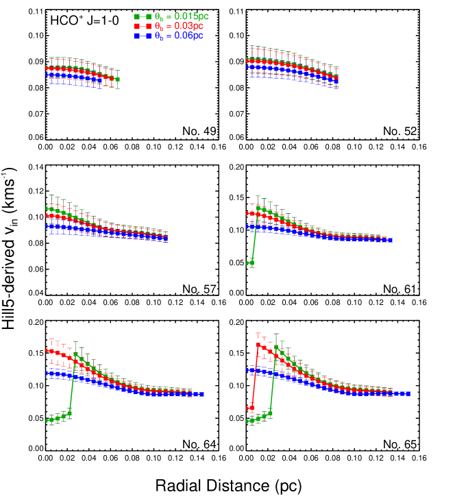
Figure 6: The Hill5-derived infall velocities along multiple LOSs through the core from its center to a position $\sim~{}$0.18 pc radially offset from the center. We examine six snapshots in the core evolution using the HCO⁺ $J=1-0$ rotational transition and three values for $\theta_{\rm b}$: 0.015 pc ($green$), 0.03 pc ($red$) and 0.06 pc ($blue$). Error–bars for the plotted values correspond to the $NRMSD$–value for each Hill5–fitted spectrum. Artificial drops at the center in several of the plots for the narrowest beamwidth correspond to poorly fitted saturated spectra where the central density far exceeds the transition $n_{\rm cr}$.

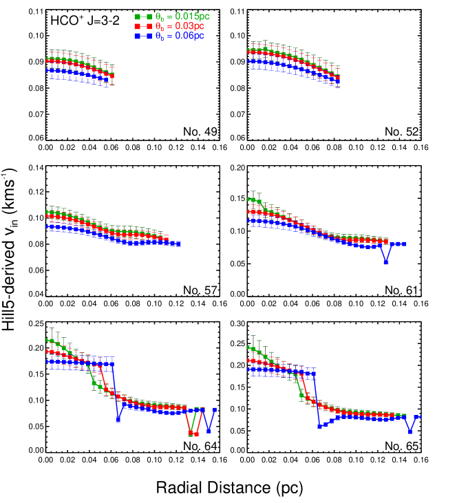
Figure 7: The Hill5-derived infall velocities along multiple LOSs through the core from its center to a position $\sim 0.18$ pc radially offset from the center. We examine six snapshots in the core evolution using the HCO⁺ $J=3-2$ rotational transition and three values for $\theta_{\rm b}$: 0.015 pc ($green$), 0.03 pc ($red$) and 0.06 pc ($blue$). Error-bars for the plotted values correspond to the $NRMSD$–value for each Hill5-fitted spectrum. Unlike the $J=1-0$ transition, $J=3-2$ does not suffer from the artificial drops for small $\theta_{\rm b}$. However, for the later stages of the simulation, where the velocity field increases steeply at the center of the core, the larger beam of $\theta_{\rm b}=0.06$ pc samples the field too coarsely, resulting in abrupt changes in its $v_{\rm in}^{Hill5}$–radial plots (after snapshot 57) compared to narrower $\theta_{\rm b}$–values.

3.3 $T_{\rm b}/T_{\rm r}$ ratio

As mentioned in the Introduction, another indicator of infalling motions is the degree of blue/red asymmetry observed in a sufficiently optically thick line. The asymmetry is quantified by determining the ratio of the blue to red peaks, or $T_{\rm b}/T_{\rm r}$ (e.g., see Sun & Gao, 2009). A blue profile requires $T_{\rm b}/T_{\rm r}>1.0$, i.e. the blue peak is stronger than the red peak, while $T_{\rm b}/T_{\rm r}<1.0$ implies a red profile. Since all of our optically thick synthetic spectral positions show two clear peaks, we computed $T_{\rm b}/T_{\rm r}$ at selected positions in the spectral maps for the selected snapshots in each of the HCO⁺ $J=1-0$ and $J=3-2$ rotational transitions. $T_{\rm b}$ and $T_{\rm r}$ are simply the values of the blue and red peak emissions, in Kelvin, from each synthetic spectrum, respectively. Spectra displaying large values of this ratios can appear in the form of a strong blue component with a relatively weaker shoulder. We analyse the optically thick synthetic spectra in terms of this ratio with the results presented in §4.2.3 and displayed in figs. 8 and 9.

4 Results

4.1 Comparison of line profile-derived speeds with actual physical speeds

From the radial plots of figs. 6 and 7 (see also the example spectra in fig. 2), the inferred infall motions are seen to be subsonic in most cases, for both transitions, in spite of the actual maximum infall speeds in the simulation being supersonic (see Table 1), up to Mach numbers of nearly 3. Our inferred infall speeds using the Hill5 method range from $\sim$ 0.07 to 0.24 ${\rm km\ s}^{-1}$ at the center of the collapse for the studied snapshots, becoming marginally supersonic at the final snapshot only. Additionally, a simple inspection of the line profiles shows that the separation between the blue peak and the absorption minimum of the line lies between 0.15 and 0.2 ${\rm km\ s}^{-1}$, thus being perfectly consistent with reported infall speeds derived from blue-skewed asymmetric profiles (e.g., Lee et al., 2001; Campbell et al., 2016). This implies that the standard modeling of blue-asymmetry line profiles underestimates the infall speeds by factors of up to $\sim 3$–4.

4.2 Radial variation of derived core parameters

In this section, we examine the radial variation of the aforementioned parameters at various timesteps in the simulation as the LOS is shifted from the core center to a position $\sim$ 0.18 pc from the center. We also examine the variability in the determined parameters with the value of $\theta_{\rm b}$, i.e. the effects of beam-averaging.

4.2.1 Radial variation of $\delta v$

In figs. 3 and 4, we plot the variation of the asymmetry parameter, $\delta v$, with radial offset for HCO⁺ $J=1-0$ and $J=3-2$, respectively. In these plots, we consider beamwidths of 0.015 pc, 0.03 pc and 0.06 pc, respectively, for each of the analyzed snapshots. As line saturation occurs at all frequencies over a lineshape function, the radial profile of this parameter can be affected at small radial offsets where the density and hence optical depth increase significantly towards the end of the simulation (see §5.1 for an in-depth discussion of line saturation).

4.2.2 Radial variation of $v_{\rm in}^{Hill5}$

In fig. 2 we display the HCO⁺ $J=3-2$ synthetic spectra from the LOS-projected core at 5 different radial positions, namely the central position as well as four neighboring positions at increasing distances from the core center (with a constant separation of 0.045 pc) for snapshots 52 (fig. 2(a)) and 61 (fig. 2(b)), respectively. For both sets of profiles, we take $\theta_{\rm b}=0.03$ pc. An overlaid best-fit hybrid Hill5 model as well as the isolated N₂H⁺ hyperfine component are also included for each position. To quantify the quality of each fit, we display the estimated infall velocity from the hybrid Hill5 model, $v_{\rm in}^{Hill5}$, the $NRMSD$–value of the fit, and the value of $\sigma_{\rm los}$ from the isolated N₂H⁺ hyperfine component.

The radial dependence of the Hill5-derived infall velocity ($v_{\rm in}^{Hill5}$) for both the HCO⁺ $J=1-0$ and $J=3-2$ transitions, is plotted for all snapshots in figs. 6 and 7, respectively. The synthetic beamwidths, $\theta_{\rm b}$, of 0.015 pc (green), 0.03 pc (red) and 0.06 pc (blue) are plotted together for a number of radial offsets from the core center for each snapshot in the two transitions. We have also converted the $NRMSD$–values from each best-fit Hill5 model into an associated error of the fit and plot these errors in the form of error bars for all analysed positions in figs. 6 and 7.

At this point we should note that there is an unresolvable degeneracy between the optical depth in a line profile and either the brightness ratio of its peaks ($T_{\rm b}$/$T_{\rm r}$) or their velocity separation. That is to say, as the optical depth increases, the separation of the peaks becomes unrelated to the actual velocity of the gas within the beam. However, as we clearly demonstrate in the radial plots for $v_{\rm in}^{Hill5}$ in figs. 6 and 7, very optically thick or saturated spectral positions have high $NRMSD$-values in our analysis and, though presented, are considered unreliable data.

4.2.3 Radial variation of $T_{\rm b}/T_{\rm r}$

The variation in $T_{\rm b}/T_{\rm r}$ with radial distance from the core center for snapshots 49 ($t=1.45\,t_{\rm ff}$, top row), 57 ($t=1.71\,t_{\rm ff}$, middle row) and 65 ($t=2.14\,t_{\rm ff}$, bottom row) is presented in fig. 8 (HCO⁺ $J=1-0$) and fig. 9 (HCO⁺ $J=3-2$) for $\theta_{\rm b}=0.015$ pc (left), 0.03 pc (center) and 0.06 pc (right), respectively. As an aside, for snapshot 57 at $\theta_{\rm b}=0.015$ pc for each transition, we determined $T_{\rm b}/T_{\rm r}$ at the limiting spatial resolution of the input grid, i.e. at every voxel along a radial arm from the center to the edge of the $256^{3}$ subgrid. The derived variation, showing a superposed secondary spurious peak pattern for each transition, is indicative of the limiting spatial resolution of the simulation.

Figure 8: Variation of $T_{\rm b}/T_{\rm r}$ (see §3.3) with radial distance from core center using HCO⁺ $J=1-0$ for snapshots 49 ($t=1.45\,t_{\rm ff}$, top row), 57 ($t=1.71\,t_{\rm ff}$, middle row) and 65 ($t=2.14\,t_{\rm ff}$, bottom row) for the $J=1-0$ transition of HCO⁺ for $\theta_{\rm b}=0.015$ pc (left), 0.03 pc (center) and 0.06 pc (right), respectively.

Figure 9: Variation of $T_{\rm b}/T_{\rm r}$ (see §3.3) with radial distance from core center using HCO⁺ $J=3-2$ for snapshots 49 ($t=1.45\,t_{\rm ff}$, top row), 57 ($t=1.71\,t_{\rm ff}$, middle row) and 65 ($t=2.14\,t_{\rm ff}$, bottom row) for the $J=1-0$ transition of HCO⁺ for $\theta_{\rm b}=0.015$ pc (left), 0.03 pc (center) and 0.06 pc (right), respectively.

5 Discussion

5.1 Comparison with previous observational studies

In §4 we have provided a testable framework for the hierarchical collapsing core model by means of analyzing its synthetic spectra in commonly observed species. Our findings can be directly compared with existing observed spectral maps to place a firmer understanding on the dynamics in star-forming cores.

Specifically, we have analyzed the synthetic spectra determined for a number of snapshots within the last 25% of the evolution of an isothermal, spherically symmetric, hierarchically collapsing core, the last of which corresponds to a time immediately prior to protostellar formation. With this simple model of a collapsing core in a gravitationally unstable envelope, we can reproduce the blue-skewed asymmetric line profile indicative of collapse motions. We find, like Zhou et al. (1993), that this signature is visible also in higher excitation rotational lines.

On the other hand, Zhou (1992, hereafter Z92) found an extended line profile signature (or “extended wing emission”) in a synthetic LP-model and concluded that the LP model was unrealistic, as this signature is generally not observed. However, it has been suggested that the microturbulent model used by Z92 artificially broadened his synthetic line profiles (Masunaga & Inutsuka, 2000). We can support this assertion since our numerical model, without the microturbulent component, produces no such broadening. Thus, the unrealistic component of Z92’s model may have been the addition of a microturbulent component, not the underlying LP flow regime.

Our main result is that the infall speeds derived from the line profiles using simple models are systematically lower than the actual maximum speeds arising in the numerical model. This mismatch occurs because the outside-in radial velocity profile that self-consistently develops in the simulation is very different from the inside-out collapse assumed by Shu (1977), which has often been used as a template radial velocity profile for the interpretation of line profiles. Instead, in outside-in collapse, the highest velocities occur in the core’s envelope during the prestellar stage; that is, at radii where the density is decreasing, while the densest parts of the core coincide with the lowest infall speeds further inwards. Therefore, since the optically thin parts of line profiles are essentially density-weighted velocity histograms (e.g., Pichardo et al., 2000), the largest velocities are down-weighted by the lower densities, thus represented by reduced emission within the line, while lower velocities have a larger weighting and dominate the blue and red peaks, as well as the absorption dip of the profile.

Quantitatively, the difference between the actual peak velocity for each snapshot in Table 1 and the corresponding $v_{\rm in}^{Hill5}$ (from figs. 6 and 7) for the central position ranges from (earliest-latest): 1.5-.3.5 ($\theta_{\rm b}=0.015$ pc), 1.5-3.8 ($\theta_{\rm b}=0.03$ pc) and 1.6-4.5 ($\theta_{\rm b}=0.06$ pc) for HCO⁺ $J=1-0$; and 1.4-2.3 ($\theta_{\rm b}=0.015$ pc), 1.5-2.7 ($\theta_{\rm b}=0.03$ pc) and 1.5-3.0 ($\theta_{\rm b}=0.06$ pc) for HCO⁺ $J=3-2$. From this, we can deduce that higher transitions are more accurate in estimating the actual core velocity than lower transitions for a given species (see also §5.3) and that the variation between $v_{\rm in}^{Hill5}$ and the actual peak velocity in the core increases as the core evolves. Also, larger beams dilute the measured signal resulting in lower values of $v_{\rm in}^{Hill5}$.

Moreover, we find that the inferred infall speeds appear to increase as the LOS intersects the core closer to its center. This is probably due to the fact that, for LOSs farther from the center, the LOS component of the radial infall motions is smaller (Anglada et al., 1987). This is consistent with interferometric observations of actual cores displaying extended inward motions (e.g. L1544, L694-2 and NGC 1333 Tafalla et al., 1998; Williams et al., 2006; Walsh et al., 2006), which show that the inward speeds in such cores decrease with increasing projected radius.

We also note that we did not have to consider a static envelope in order to create the self-absorption. Instead, in our case the self-absorption is produced by the core’s centermost regions (see right panel of fig. 10), which have the lowest velocities and the highest opacities. This is evidenced by the fact that we are only considering half of the numerical box for the generation of the line profiles using MOLLIE, so that the borders of the region considered have velocities that are typically not less than half the maximum infall speeds (see the top panel of fig. 1, where the borders of the region considered for the radiative transfer calculation are marked by vertical dashed lines), so that this material cannot be causing the absorption of the near-zero velocity emission.

We should also note that, due to the larger central densities towards the end of the simulation, the self-absorbed spectrum begins to saturate for spatial positions close to the core center. It becomes broader and diminishes relatively in brightness compared to spectra observed towards neighboring less dense positions. This spectrum therefore departs from the typical infall signature that is apparent at spatial positions largely separated from the center (e.g. compare the spectral panels for snapshot 61 in fig. 2(b)). An attempted Hill5 model fit contains spurious fitted points resulting in a relatively poorer approximation to the underlying saturated spectrum and hence a higher $NRMSD$–value. In actual spectral data, low-lying rotational transitions naturally saturate when the density far exceeds their $n_{\rm cr}$ for excitation, especially for narrower $\theta_{\rm b}$, and so too depart from the typical infall signature. Thus, we infer that low-$n_{\rm crit}$ transitions suffering from saturation may prove inadequate for correctly capturing the infall process.

For small radial offsets in fig. 6, corresponding to $\theta_{\rm b}=0.015$ pc (green datapoints), the derived infall velocities drop abruptly relative to those further out as a result of the sensitivity of the Hill5 algorithm to the line profile shape - that is, its inability to fit saturated lines. Comparing the resulting fitted data values with the corresponding values for HCO⁺ $J=3-2$ in fig. 7, it can be seen that saturated lines are unreliable when trying to derive infall velocities. Saturation is lessened by increasing the width of the synthetic beam by causing a greater fraction of the infalling material to be sampled. Analogously, far from the core center, the relative shallowness of the self-absorption dip becomes more prominent as the $T_{\rm b}$/$T_{\rm r}$–ratio declines, again resulting in an artificial drop in $v_{\rm in}^{Hill5}$. The point where this appears is progressively further away from the center as the core evolves and is reflected in the number of datapoints included for each snapshot. As can be seen from the corresponding sets of plots for the two transitions, the magnitudes of the derived velocities differ on account of a number of factors: choice of molecular transition (i.e. $n_{\rm cr}$), proximity to core center and the evolutionary state of the core (see also Keown et al., 2016). Also, from figs. 6 and 7, a successively wider $\theta_{\rm b}$ results in a slightly reduced $v_{\rm in}^{Hill5}$ for small impact parameters relative to the core center. This effect is due to larger beams sampling a greater fraction of relatively slower moving gas and lessens further from the center as a result to the relative drop in velocity at all positions for large impact parameters.

In all modeled spectral positions, the weaker red peak never resembles a red shoulder to the stronger blue peak, and is nonetheless significant. The red shoulder feature in line spectra has been associated with very large infall velocities (so-called “fast” infall, Myers et al., 1996, DM05) and is ill-fitted by the Hill5 model. Thus, the large $NRMSD$–values are solely due to saturation in the modeled synthetic spectral data. The range of differences between the respective infall velocities determined using the different values of $\theta_{\rm b}$ is (excluding errors) $0.003~{}\lesssim~{}\delta v_{\rm in}^{Hill5}~{}\lesssim~{}0.05$ ${\rm km\ s}^{-1}$, from non-saturated spectral positions and amongst all analysed snapshots. Among the different values of $\theta_{\rm b}$, for each transition and snapshot investigated, we find that the derived $v_{\rm in}^{Hill5}$ does not vary appreciably for non-saturated ($\sim 15$%), in reasonable agreement with DM05.

5.2 Analytical solutions to the spherical collapse problem and the origin of the infall profiles in prestellar cores

Our main result (c.f. §4.1) is that standard analysis techniques of the infall profiles in moderately optically thick lines of collapsing cores tend to systematically underestimate the speeds occurring in the cores. This result has profound consequences on our understanding of the dynamical state of prestellar cores, and thus it is important to understand the origin of this effect.

5.2.1 Discussion of spherical collapse models

In order to understand the reason for this sytematic underestimation of the infall speed by standard analysis methods of line profiles, it is necessary to discuss the nature of the velocity profile arising in our simulation, in comparison to the standard “inside-out” velocity profile assumed in most models for infall line profiles.

The velocity profile arising in our simulation is of the “outside-in” kind (e.g., Gong & Ostriker, 2009, 2011, Paper I). By “outside-in” we refer to a flow described by “Band 0” in the parameter-space analytical study of Whitworth & Summers (1985, hereafter WS85), which corresponds to strongly gravitationally unstable initial conditions. This class of collapse flow includes the standard Larson-Penston solutions (Larson, 1969; Penston, 1969), and is appropriate for our simulation, in which the whole numerical box is strongly gravitationally unstable. This type of flow is characterized by an asymptotic solution consisting of a central part with a roughly uniform density profile, surrounded by an $r^{-2}$ power-law envelope, resembling the radial density scaling of a BE sphere, although with a higher absolute value of the density than that required for hydrostatic equilibrium (e.g., Keto et al., 2015, Paper I). For this configuration, the infall speed increases linearly with radius at the central regions and approaches a supersonic constant value at the outer envelope. Indeed, the numerical simulation approaches this regime (see fig. 2 of Paper I). The transition between the core and the envelope occurs at a radius of the order of the Jeans length for the central density and temperature (Keto & Caselli, 2010).

This flow structure is in sharp contrast with the standard assumption that the velocity profile has an inside-out nature (e.g., Shu, 1977; Evans, 1999), in which the infall speed is maximum at the center, has an $r^{-1/2}$ radial dependence, and extends only to a rarefaction front located at a radius $R_{\rm Shu}=c_{\rm s}t_{\rm PF}$, where $t_{\rm PF}$ is the time since the formation of the singularity (the protostar). Beyond this radius, the inside-out Shu profile assumes that the gas is still in a hydrostatic state. This radial velocity profile is applicable only for the protostellar stage (i.e., after the formation of the singularity—the protostar), and only for an initial condition given by a SIS at the time of protostar formation. This idealized initial condition assumes that the prestellar evolution of the core proceeds quasistatically all the way to the formation of the SIS, and only becomes fully dynamic after this time.

Shu (1977) argued that the SIS hydrostatic initial condition should be possible as long as the flow is subsonic, so as to allow the establishment of detailed pressure balance at all radii. Furthermore, he argued that the initial and boundary conditions of the Larson-Penston similarity solutions were highly numerically ad-hoc; i.e., chosen to match their numerical results. Furthermore, he argued that the smoothly (i.e., without a shock), monotonically-decreasing velocity profile towards the center could only be made consistent with the outer supersonic inflow through “an artificial arrangement of self-gravity and pressure gradient”.

However, shortly thereafter, (Hunter, 1977) showed that numerical simulations in general seemed to be best described by the Larson-Penston similarity solution. The simulation from Paper I, which starts with a generic Gaussian fluctuation superposed on a uniform medium also approaches this type of flow. Moreover, Whitworth et al. (1996) and Vázquez-Semadeni et al. (2005) have later suggested that actually it is the SIS that is most unlikely. This is because the SIS is an unstable equilibrium solution, and moreover, any previous equilibrium solution of the form of a truncated BE sphere with a central-to-peripheral density contrast larger than the critical value of $\sim 14$ is unstable as well (Ebert, 1955; Bonnor, 1956), so that the SIS is actually the most possibly unstable case of the family of hydrostatic solutions represented by the Lane-Emden equation. As such, the SIS as a quasistatic initial condition for spherical collapse is unrealizable in practice.

It is nevertheless very important to note that the infall velocity ideally remains constant at arbitrarily large distances from the core’s center in the outside-in collapse of a uniform-density medium. In practice, however, this asymptotic solution cannot occur, because the cloud must end at some point, and the density must decrease again, or at least be characterized by a density gradient, albeit perhaps weaker than that in the core. Moreover, the analytic solution (Whitworth & Summers, 1985) does not consider the fact that the fluctuation may be embedded in an already contracting cloud, so that the gas flows towards the large-scale collapse center (different from the core’s center), as in the “conveyor-belt” flows observed in realistic cloud simulations (Gómez & Vázquez-Semadeni, 2014) and in the Central Molecular Zone of The Galaxy (Longmore et al., 2014). On top of this flow, the density fluctuation (perhaps produced by turbulence) eventually becomes unstable as the average Jeans mass in the whole cloud decreases due to the global contraction, and begins to collapse towards its own center. In our simulation, the decrease of the infall speed towards the edge of the box is an artifact of the periodic boundary conditions, but this mimics the effect seen in large-scale simulations that the local collapses within the cloud extend to finite distances only, because of the finite size of the turbulent density fluctuations.

In any case, the extent of the collapsing region in the outside-in collapse case is much larger than the extent of the standard rarefation front of Shu’s (1977) inside-out collapse, $R_{\rm Shu}$ (see above). This is because the rarefaction front in Shu’s inside-out collapse has not even started to propagate over the entire duration of our simulation, since it precisely starts at the ending time of the simulation (i.e., at the time of formation of the singularity). This explains the “extended inwards motions” observed in actual cores, which extend far beyond the position consistent with Shu’s rarefaction front.

5.2.2 The formation of the line profile for outside-in velocity profiles

In the left panel of fig. 10, we show the “standard picture” (Evans, 1999) to explain the self-absorbed line profile signature on the basis of the inside-out collapse model of Shu (1977). In the right panel of this figure, we show the corresponding schematic diagram reflecting our interpretation of this phenomenon, on the basis of the outside-in collapse characteristic of our numerical simulation. In each panel, the observing antenna is located to the right of the schematic with its LOS passing through the circular core from right to left.

As seen in the left panel of fig. 10, the structure of the core assumed by Evans (1999) is that of Shu’s (1977) inside-out collapse, with a central infalling core and an outer hydrostatic envelope, mediated by an expanding rarefaction front located at radius $R_{\rm Shu}$ (cf. §5.2.1). In this picture, the central absorption dip in the line profile is caused by the outer static envelope.

Instead, as shown by the right panel of fig. 10, for the outside-in profile, there is no outer hydrostatic envelope, and the outer envelope infalls at speeds ranging from the maximum to roughly half that value (cf. dashed portions of  fig. 1). In this case, the central absorption dip is produced by the high-opacity, low velocity material near the core center, while the envelope’s velocity appears in the line profile wing, downweighted by the lower density there. As mentioned in §5, the fact that the absorption dip is caused by the dense central parts of the core is evidenced by the fact that we are only considering the central half of the simulation in each direction, so that the gas is still moving with supersonic infall velocities at the boundary of this region. Thus, the only material with near-zero velocity is at the core center.

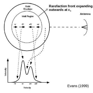
(a) Inside-out collapse picture of line asymmetry

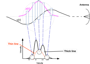
(b) Outside-in collapse picture of line asymmetry

Figure 10: Schematic representations of how various parts of the star-forming mechanisms of (a) inside-out (from Evans, 1999) and (b) outside-in collapse (this work) contribute to the self-absorbed optically thick line profile. In (b), we highlight, using rectangular sections of $\tau_{\nu}\sim 1$, specific parts for a given snapshot of each of its density (magenta) and velocity (black) profiles that give rise to characteristic features of the self-absorbed line. With time, the peak velocity increases and is more centralized with the mean velocity of the material, responsible for the line self-absorption, shifting to redder velocities and therefore displacing the self-absorption minimum to these velocities too. Also in (b), a representative optically-thin line is included as emanating from the center of the collapse for a high $n_{\rm crit}$ transition. In each panel, the antenna is positioned to the right with its LOS passing through the circular core from right to left.

5.2.3 Comparison with previous work

Synthetic observations of various numerical models of spherically-symmetric collapse have been previously presented by Keto et al. (2015, hereafter K15), to determine which type of collapse model best matches the observed line profiles of the L1544 starless core. In particular, those authors considered the cases of a quasi-equilibrium BE sphere (QE-BES), a non-equilibrium BE sphere (NE-BES), a static sphere, a Larson-Penston (LP) flow, and the inside-out collapse of an SIS as modeled by Shu (1977). They concluded that the QE-BES regime produces synthetic line profiles that best match those observed in the L1544 core.

Interestingly, the evolution of the QE-BES of K15 does have some similarities with that of our collapsing core embedded in an unstable uniform medium. The QE-BES model was constructed by K15 as an unstable BES, and then slightly perturbed, to allow it to evolve hydrodynamically. Although K15 refer to the collapse mode of the QE-BES as “inside-out”, it also presents the inner region in which the infall speed increases linearly with radius, so it falls into our description of “outside-in” collapse. Because of their setup, it also has an outer radius beyond which the infall velocity begins to decrease outwards. However, due to the setup as a perturbed marginal equilibrium, it develops speeds slightly slower than an alternative experiment with an out-of-equilibrium setup, labeled NE-BES by K15: while the QE-BES shows infall speeds $\sim 0.2\ {\rm km\ s}^{-1}$ (i.e., $\sim c_{\rm s}$) at the last timestep shown, the NE-BES develops speeds $\sim 0.25\ {\rm km\ s}^{-1}\sim 1.25\ c_{\rm s}$ at the same time. However, K15 do not indicate how far from the appearance of the singularity are those times, so it is not possible to know whether supersonic speeds do appear at later times in the QE-BES case as well.

Similarly to this work, K15 compare optically-thick H₂O ($J_{K_{\rm a}K_{\rm c}}=1_{10}\rightarrow 1_{01}$) and optically thin C¹⁸O ($1\rightarrow 0$) line observations of the L1544 core against synthetic observations in the same lines of their numerically simulated cores. They conclude that the QE-BES provides the best match to the observed profiles. However, K15 concentrate on matching the observed line profiles, rather than on comparing the actual infall speeds in the numerical model to the speeds that would be inferred from the line profiles using standard line-modeling techniques, which is our main interest here.

K15 devote a full section to justify the feasibility of stable BE spheres forming within a turbulent molecular cloud environment before becoming unstable and proceeding to dynamical collapse. They essentially follow Field et al. (2011) and “imagine the ISM as a turbulent cascade of mass and energy from larger to smaller scales”, in which the larger structures contain supersonic motions and thus fragment, while the smaller structures (“cores”) are subsonic and thus do not fragment any further (see also Vázquez-Semadeni et al., 2003). Then K15 assume that a fraction of these subsonic cores can be stabilized by the combined effect of thermal and turbulent energy, and that, as the turbulent energy dissipates, the cores can go into collapse. They also suggest that cores that are supported by thermal energy alone may never form stars, and that many of the cores in the Pipe nebula may be in this category, referring to the result by Lada et al. (2008) that most of the cores in the Pipe appear to have masses smaller than their Bonnor-Ebert mass, and therefore must be gravitationally stable, and confined by an external pressure.

This scenario, however, does not appear feasible in practice. First, as already stated in §1.1, for a BE sphere to be stable, besides having a central-to-peripheral density contrast smaller than the critical value, it must be truncated and embedded in a diffuse, warm medium, which provides pressure without adding weight (Vázquez-Semadeni et al., 2005). Cores deep inside molecular clouds are likely to be embedded in the same molecular material as that which they are made of, and therefore the tenuous confining medium is not available. In this case, a local density enhancement (a “core”) is also a local pressure enhancement, and must therefore re-expand in a sound-crossing time, if it does not become locally Jeans-unstable (Galván-Madrid et al., 2007).

Second, in Paper I we showed that our collapsing core, throughout its evolution, tracks the locus of the Pipe cores in the diagram of $M_{\rm c}/M_{\rm BE}$ versus $M_{\rm c}$, where $M_{\rm c}$ is the core’s mass and $M_{\rm BE}$ is its BE mass, including the region occupied by the apparently stable cores. This occurs precisely because our core is just “the tip of the iceberg” of a larger-scale collapse that extends out to the uniform background. Since this uniform background is generally not considered part of the core, the core may appear stable, because not all the mass involved in the collapse is accounted for. The infall motions that extend into the uniform background constitute an accretion flow from the cloud onto the core which, however, cannot be described by a simulation of a core artificially truncated at some radius.

Finally, to our knowledge, no numerical simulation of a turbulent cloud has ever reported the production of quasi-equilibrium structures. K15 refer to the statement by Offner et al. (2008) that “the protostellar cores in the simulations are at the centers of regions of supersonic infall, which contradicts the observations that show at most transonic contraction” (see also Mohammadpour & Stahler, 2013), suggesting that this may be a problem of the simulations. However, it should be noted that the statement by Offner et al. (2008) refers to protostellar cores, for which supersonic speeds are more commonly observed, and the discrepancy they discuss is more quantitative than qualitatve. In fact, those authors offer the explanation that their simulations lack stellar feedback that may prevent the development of the very massive stellar particles, and thus the excessive speeds developing in their protostellar cores.

Mohammadpour & Stahler (2013), on the other hand, do refer specifically to the supersonic speeds that develop in simulations shortly before the formation of the protostar (i.e., still during the prestellar stage), and they conclude that this is indicative of some physical mechanism that is missing from the simulations, which is required to bring them into concordance with observations. Our result, that the apparently subsonic nature of the prestellar collapse may be simply the result of a misinterpretation of the infall line profiles because of the assumption of an erroneous infall velocity radial profile, suggests that the problem may lie in the interpretation of the observations rather than in the simulations.

Instead, our mechanism of global hierarchical gravitational collapse of MCs (Vázquez-Semadeni et al., 2009; Ballesteros-Paredes et al., 2007, see also Vázquez-Semadeni 2018, in preparation) provides a simple mechanism through which a density fluctuation (probably of turbulent origin) can at some point become gravitationally (Jeans) unstable, and begin to collapse. Succintly, this is just the result of the global reduction of the average Jeans mass in the cloud as it contracts gravitationally (Hoyle, 1953), so that fluctuations of a given mass are stable as long as their mass is lower than the mean Jeans mass, but, as this mass decreases over time, they eventually become unstable and begin to collapse. When this happens, their mass will be just marginally above the mean Jeans mass in the cloud, similarly to the case of K15’s QE-BES.

5.3 Beamwidth dependence of the profile asymmetry

We now turn to the origin of the different degrees of asymmetry in observational line spectra based on a number of factors including incident observational beamwidth, molecular transition and proximity of incident beam to core center. The dependence of the $T_{\rm b}/T_{\rm r}$–ratio on both time and radial offset from core center is considered in figs. 8 and 9. In this work, we do not consider depletion, and allow the emission profiles to develop naturally for both rotational lines.

As previously discussed, within the quasi-static contraction picture, star-forming cores oscillate globally and at the point of gravitational instability, the fundamental oscillation mode has zero frequency. Stahler & Yen (2009, 2010) studied, using perturbation theory, the evolution of a 3$M_{\odot}$ spherical cloud with such a frozen mode. They found that their cloud underwent accelerated, though subsonic, contraction for a period of $\sim$ 1 Myr. Although their resulting line spectra were mildly asymmetric, they concluded that the accelerating character of their model naturally explained why low density starless cores exhibit line spectra with smaller $T_{\rm b}/T_{\rm r}$–ratios. However, unlike in this work, their model was unable to account for the extended spatial occurrence of asymmetric line profiles (Stahler & Yen, 2010).

Instead, in our synthetic observations of the simulated collapsing core, this ratio is consistently higher for HCO⁺ $J=3-2$ than for $J=1-0$ if we compare corresponding panels in figs. 8 and 9 for small radial offsets from the core center. In fact, from the panels, where $\theta_{\rm b}=0.06$ pc, the difference grows as the core evolves. The $J=3-2$ emission is more centrally confined than the $J=1-0$ emission on account of its larger $n_{\rm cr}$ (see Table 2). Thus, for the more centrally dense core snapshots considered here, the increasing infall velocity (as the core evolves) is more apparent for the higher transition because the mean density sampled by the respective values of $\theta_{\rm b}$, for each snapshot, is maintained within its $n_{\rm cr}$ while it exceeds the $n_{\rm cr}$ of HCO⁺ $J=1-0$, evidenced by saturation at small $\theta_{\rm b}$ for the latest snapshots ($T_{\rm b}/T_{\rm r}<1.0$ at $\theta_{\rm b}=0.015$ pc for snapshot 65 in fig. 8). Since HCO⁺ $J=3-2$ does not succumb as easily to saturation as the $J=1-0$ line, it produces stronger a $T_{\rm b}/T_{\rm r}$ ratio resulting in a higher derived $v_{\rm in}$.

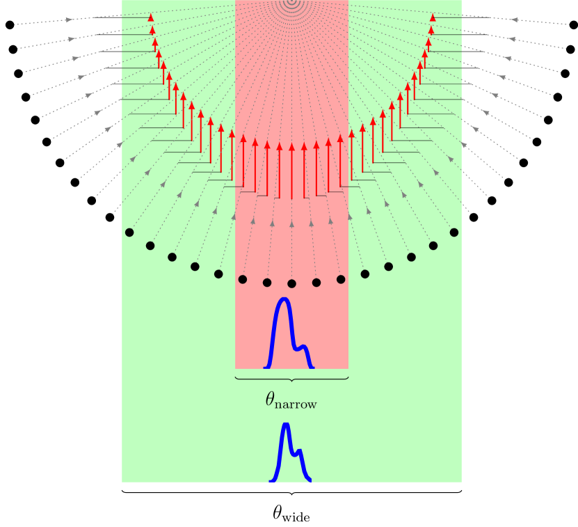
Figure 11: Simple diagram explaining the detection of larger $T_{\rm b}/T_{\rm r}$–ratios for collapsing core gas (black dots of equal velocity). $\theta_{\rm wide}$ captures a larger fraction, by volume (in green), of the emission from infalling gas along the LOS through the core center, while $\theta_{\rm narrow}$ captures a smaller, localized volume (in pink). From the diagram, $\theta_{\rm narrow}$ traverses infalling gas traveling mainly parallel to the LOS (velocity components in red). $\theta_{\rm wide}$ traverses this same gas as well as gas oriented at larger angles (smaller red components) relative to the LOS. The resulting beam convolution for this detected gas of similar velocity will result in larger $T_{\rm b}/T_{\rm r}$–ratios for $\theta_{\rm narrow}$. This holds similarly for the detection of large $T_{\rm b}/T_{\rm r}$–ratios far from the core center using a wider beam.

For each transition, at small offsets from the center, $T_{\rm b}/T_{\rm r}$ is seen to decrease as $\theta_{\rm b}$ is increased (for non-saturated positions). The common explanation for this, illustrated in fig. 11, is that a wider beam passing through the core’s center picks up emission from a larger region, but in which the additional material is moving more obliquely with respect to the LOS (Anglada et al., 1987, 1991), and therefore the projection of its velocity onto the LOS is smaller. Thus, in a wider beam passing through the center, most of the gas contributes lower velocities, and therefore the $T_{\rm b}/T_{\rm r}$ ratio is also smaller while, conversely, a more compact sampling of the collapsing gas produces a more prominent line asymmetry, especially closer to the core center, again resulting in a higher derived $v_{\rm in}$ (see also figs. 6 and 7). At large radial offsets from the core center using both lines, the value of $T_{\rm b}/T_{\rm r}$ falls between 1.1 and 1.35 depending on the stage of collapse and the value of $\theta_{\rm b}$. These positions coincide with relatively quiescent core material with their $T_{\rm b}/T_{\rm r}$–values giving the impression of the presence of a static ($T_{\rm b}/T_{\rm r}\approx$ 1.0) external envelope relative to the more dynamic infalling core center.

The $T_{\rm b}$/$T_{\rm r}$ ratio is therefore very sensitive to the excitation conditions in the core. Better estimates of core infall motions are possible by observing the higher rotational transitions of commonly-observed molecular species using as finite a beam as possible.

Another very noteworthy point to make is that our synthetic spectra for the HCO⁺ $J=3-2$ transition reproduce the so-called extreme $T_{\rm b}$/$T_{\rm r}$ ratios ($\gtrsim$ 3, see last two panels of fig. 9 for snapshot 65 with $\theta_{\rm b}=0.03$ and 0.06 pc respectively), seen in the evolved collapsing collapsing sources B133 (Gregersen et al., 2000) and NGC 7538 (Sun & Gao, 2009) using similarly optically thick transitions. Since each of these cores harbors a central source (both are Class 0 cores), while snapshot 65 of the simulation represents the end of the simulated prestellar core collapse, at which point a central source is about to form, their respective velocity profiles should resemble one another (e.g. see fig. 1(a)). We therefore suggest that these particular cores are undergoing a similar physical process to that exhibited by the final stages of our simulation.

5.4 Radial variation of $\delta v$

For the asymmetry parameter ($\delta v$), in both transitions, the general consensus is that narrower beams result in smaller $\left|\delta v\right|$ at the core center but with larger values far from the center for a given snapshot. For the later stages of collapse, prior to star formation, this parameter tends to increase with increasing radial offset from the core center due to the decrease in $\Delta v_{\rm thin}$ and the inverse relationship between $\left|\delta v\right|$ and $\Delta v_{\rm thin}$. In view of the results presented here, the strict $\left|\delta v\right|>0.25$ requirement for the assignment of true collapsing motions (see Mardones et al. 1997) would need to be revised for mapped observations of evolved collapsing cores, especially for typical values of $\theta_{\rm b}$, given how $\left|\delta v\right|$ behaves very close to evolved collapse centers where $\Delta v_{\rm thin}$ is largest.

At the core center for snapshot 49, the optically thick peak for HCO⁺ $J=3-2$ is shifted blueward when compared to the same region in snapshot 52 (top two panels of fig. 4) resulting in larger values for $\left|\delta v\right|$. Since HCO⁺ $J=1-0$ does not exhibit this feature at any value of $\theta_{\rm b}$, this may indicate that the higher transition is more sensitive to the velocity field at comparatively lower densities. Differing velocity field gradients in the detected emission lead to variations in the position of the emission peak. Narrower beamwidths are more sensitive to such variations and so a $\delta v$–analysis of mapped spectral regions can be used to identify gradients in the velocity field.

Given the form of eq. (1), a numerical analysis of this parameter is limited by the velocity resolution of the radiative transfer setup. Nevertheless, we have been able to make some useful deductions from such an analysis of the synthetic spectra.

5.5 Radial variation in the optically thick line

It is also worth noting that our simulated core exhibits a behavior in the optically thick HCO⁺ $J=3-2$ line that is qualitatively very similar to that observed by P10 for NH₃(1,1) lines from the B5-1 cloud core as the impact parameter of their LOSs was increased (see their fig. 3 and compare to our fig. 2). These authors noted that the NH₃ line towards this core, with its blue-skewed, double-peaked asymmetry, became weaker and its central dip tended to disappear as the impact parameter was increased. This “line” actually consists of 8 magnetic hyperfine components due to the combined coupling of the magnetic hyperfine interaction of the three identical ¹H-nuclei and the quadrupolar moment of the ¹⁴N-nucleus in NH₃ (e.g., see Kukolich, 1967).

P10 interpreted the combination of the two peaks as the blending of these underlying hyperfine components. Using those components, they fitted the central NH₃ line for several individual pointings observed towards the core. From their fit, they concluded that the linewidth of each of the hyperfine components in the fit decreased as the impact parameter decreased—an indication of a “transition to coherence” (i.e., a reduction of the turbulent velocity dispersion) as the impact parameter decreased. Further, they suggested that the gradual merging of the two peaks as the impact parameter is increased is a manifestation of an increasing turbulent component that becomes wider than either of the two peaks, eventually incorporating both of them at sufficiently large values of the impact parameter. However, it is noteworthy that the overall linewidth of the line does not vary – the interpretation of an increasing turbulent component at higher impact parameters was based exlusively on the gradual disappearance of the central dip and the peaks, leaving behind a single line that has approximately the same width as the double line seen at smaller impact parameters.

On the other hand, our HCO⁺ line does not contain a discernible hyperfine structure unlike NH₃, and our simulation does not include turbulence, yet the observed behavior of the line is qualitatilvely very similar to that reported by P10. In our case, the interpretation must be that, as the impact parameter of the LOS is increased, the LOS ceases to pick up the high-density, low-infall velocity at the center, which makes up the central absorption dip, and only picks up the higher-velocity infalling gas, although at a higher angle with respect to the LOS, so the net velocity traced by the linewidth remains nearly constant. Also, the absolute intensity of the line decreases because of the drop in density at larger impact parameters. In a future contribution we will examine in detail the NH₃ line with its hyperfine structure, but it is tempting to speculate that the observed behavior of the NH₃ line reported by P10 may be due to the process we describe, rather than to a transition to coherence.

6 Summary and Concluding Remarks

We have produced synthetic spectra for the HCO⁺ $J=1-0$ and $J=3-2$, as well as the N₂H⁺ $J=1-0$ transitions for a number of snapshots of an idealized numerical simulation of the collapse of a gaussian density fluctuation with spherical symmetry immersed in a strongly gravitationally unstable background medium, within the context of the hierarchical gravitational collapse of molecular clouds (Vázquez-Semadeni et al., 2009). The simulation was presented in Naranjo-Romero et al. (2015, Paper I), and started from a minor, Jeans-sized fluctuation of amplitude 50% above the density of the uniform background, so the density and velocity fields of the simulation developed self-consistently. We examined 7 snapshots covering the time elapsed since the density fluctuation had a density contrast of $\sim 3$ with respect to the background to when this contrast was $\sim 2000$.

The main motivation for the present study was the discrepancy between the supersonic infall velocities that develop in this kind of model (e.g., Larson, 1969; Penston, 1969) and the subsonic infall speeds that are often inferred from the analysis of self-absorbed, optically-thick lines that exhibit a blue excess (e.g., Zhou, 1992; Zhou et al., 1993) and from the linewidths measured at distances $\lesssim 0.1$ pc in dense molecular cores (e.g., Goodman et al., 1998). This discrepancy has led to the general belief that dynamic collapse solutions of the hydrodynamic equations do not correctly represent the state of such cores, and that instead the cores need to be supported against their self-gravity by some agent like magnetic fields (e.g., Shu et al., 1987) or turbulence (e.g., Mac Low & Klessen, 2004; Ballesteros-Paredes et al., 2007).

However, one possible resolution of the discrepancy may lie in the very different nature of the generally assumed infall velocity profile for the interpretation of the lines and the one that develops in collapse simulations. Often, infall profiles are modeled with the assumption of a Shu (1977) “inside-out” profile, which has the highest velocities at the innermost regions of the cores and has zero velocity (i.e., remains hydrostatic) at large radial distances. This profile arises from the assumption of a singular isothermal sphere as an initial condition of the collapse. Instead, relaxation of this (unrealistic; e.g., Whitworth et al., 1996) assumption generally produces “outside-in” velocity profiles, for which the maximum speeds occur at a finite distance from the core’s center (specifically, in the core’s envelope) during the prestellar stage (e.g., Whitworth & Summers, 1985; Gómez et al., 2007; Gong & Ostriker, 2011, Paper I). In Paper I we speculated that this property of the infall velocity profile might cause a systematic underestimation of the infall speeds, because, noting that molecular line profiles are essentially density-weighted histograms of the LOS component of the velocity, such a combination of density and velocity profiles might cause the highest velocities to be down-weighted by the fact that they occur in the regions of the core where the density is already decreasing.

Our synthetic observations, and their analysis using the Hill5 method from De Vries & Myers (2005), confirm the speculation from Paper I, showing that the speeds inferred from the profiles underestimate the actual peak infall speed by factors of 2–4, thus creating the appearance of a subsonic collapse in spite of the presence of supersonic velocities in the core. This is because, contrary to the standard assumption of an inside-out infall velocity profile, our collapsing core develops an outside-in profile, in which the largest velocities occur where the density is already decreasing, thus downweighting the contribution of the fastest-moving material to the line profile. Instead, the higher weighted speeds are the inferior ones occuring near the core center, where the density is highest. It is important to remark, however, that the usage of the Hill5 method was not essential to our results: the fact that the profiles would in general be interpreted as implying subsonic speeds is clear, simply by the often-used zeroth-order approximation of measuring the velocity difference between the blue peak and the absorption dip, which in all of the spectra shown in fig. 2 is less than the sound speed.

We also found from the sets of $T_{\rm b}$/$T_{\rm r}$ radial profiles for the HCO⁺ $J=3-2$ line that this simple collapse simulation reproduces the large $T_{\rm b}$/$T_{\rm r}$–ratios observed towards a number of evolved low-mass starless and protostellar cores, contrary to the common belief that these large ratios cannot be obtained with simple models (Gregersen & Evans, 2000). By accommodating a more extended collapse incorporating both the inner core material and the outer envelope, comparatively larger infall velocities are developed in the later stages of this simple simulation than in previous setups. The simultaneity of a more extended infall pattern along the LOS together with larger magnitude infall velocities therefore enables the development of larger $T_{\rm b}$/$T_{\rm r}$–ratios.

The magnitude of the asymmetry parameter, $\left|\delta v\right|$, increases with radial offset at all times (see fig. 3 and 4). This trend is most probably associated with the emerging velocity profile at these times in the simulation and, in particular, how this profile effects the value of $\Delta v_{\rm thin}$ in eq. 1. Additionally from fig. 3-4, it can be seen that, for smaller $\theta_{\rm b}$, $\left|\delta v\right|$ is larger at small radial offsets from the center and decreases far from the core center for both HCO⁺ transitions. This is due to a narrowing of $\Delta v_{\rm thin}$ with distance from the core center, especially for later times. Saturation effects result in $|\delta v|<0.25$ for $J=3-2$ at later times, especially for spatial positions close to the core center. As we discussed in relation to the analytically derived $v_{\rm in}$ values for both $J=1-0$ and $3-2$ at later times, saturation effects appear more severe for the higher transition and are persistent even at larger values of $\theta_{\rm b}$. From this analysis, we can say that $\delta v$ is strongly dependent on the underlying velocity profile along a given LOS due to the sensitivity of $\Delta v_{\rm thin}$.

Finally, we also noted that the shape of the synthetic HCO⁺ $J=3-2$ line profiles varies with increasing offset in a qualitatively similar way to that reported by Pineda et al. (2010, P10), with the absorption dip becoming less pronounced, while the overall width of the line is unchanged. While P10 interpreted this as the consequence of the broadening of a hypothetical turbulent component towards large impact parameters that causes a blending of the blue and read peaks, in our case the lack of turbulence prevents this interpretation from being applicable. Instead, we interpreted the effect as the consequence of the fact that, as the impact parameter of the LOS increases, the LOS ceases to pick up the high-density, low-infall velocity at the center, which makes up the blue and red peaks and creates the self-absorption dip at the center, and only picks up the lower-density, higher-velocity, more distant infalling gas. In a future contribution we hope to investigate whether this scenario is applicable to NH₃ synthetic observations of our core.

We conclude that the apparently subsonic velocities generally inferred for low-mass cores, and the standard inter- pretation that they imply that the cores are not collapsing, and supported by either turbulence or magnetic fields, may be an artifact of the outside-in nature of the velocity profile that naturally arises in collapsing prestellar cores that start from realistic initial conditions, because this profile implies that the largest velocities are given less weight in the process of line formation, since they occur at large distances from the core center, where the density is lower than at the center. In addition, we have speculated that the offset dependence of the infall line profiles, with a disappearing central dip at larger offsets, may be also a consequence of the outside-in radial velocity profile rather than an indication of a “tran- sition to coherence”.

We have carried out an in-depth synthetic spectral analysis for the simple model at our disposal. Factors such as the influence of the background density on the depth of the self-absorption dip and the use of different abundance profiles could be considered for future work but do not add to the context of this paper.

References

- Alves et al. (2001) Alves J. F., Lada C. J., Lada E. A., 2001, Nature, 409, 159
- André et al. (2014) André P., Di Francesco J., Ward-Thompson D., Inutsuka S.-I., Pudritz R. E., Pineda J. E., 2014, P&PVI, 27
- Anglada et al. (1987) Anglada, G., Rodriguez, L. F., Canto, J., Estalella, R., & Lopez, R. 1987, A&A, 186, 280
- Anglada et al. (1991) Anglada, G., Estalella, R., Rodriguez, L. F., & Lopez, J. C. R. 1991, A&A, 252, 639
- Ballesteros-Paredes et al. (2007) Ballesteros-Paredes, J., Klessen, R. S., Mac Low, M.-M., & Vázquez-Semadeni, E. 2007, Protostars and Planets V, 63
- Ballesteros-Paredes et al. (2007) Ballesteros-Paredes, J., Vázquez-Semadeni, E., Palau, A., Klessen, R. S. 2018, MNRAS, 479, 2112
- Bergin & Tafalla (2007) Bergin, E. A., & Tafalla, M. 2007, ARA&A, 45, 339
- Bertoldi & McKee (1992) Bertoldi F., McKee C. F., 1992, ApJ, 395, 140
- Bonnor (1956) Bonnor, W. B. 1956, MNRAS, 116, 351
- Buisson et al. (1994) Buisson G., Desbats L., Duvert G., Forveille T., Gras R., Guilloteau S., Lucas R., Valiron P., 1994, class Manual
- Burkert & Hartmann (2004) Burkert, A., & Hartmann, L. 2004, ApJ, 616, 288
- Campbell et al. (2016) Campbell, J. L., Friesen, R. K., Martin, P. G., et al. 2016, ApJ, 819, 143
- Caselli et al. (1995) Caselli, P., Myers, P. C., Thaddeus, P., 1995, ApJL, 455, L77
- Crutcher et al. (2010) Crutcher, R. M., Wandelt, B., Heiles, C., Falgarone, E., & Troland, T. H. 2010, ApJ, 725, 466
- De Vries & Myers (2005) De Vries C. H., Myers P. C., 2005, ApJ, 620, 800 (DM05)
- Ebert (1955) Ebert, R. 1955, Zeit. für Ap., 37, 217
- Evans (1999) Evans, N. J., II 1999, ARA&A, 37, 311
- Evans (2002) Evans II, N. J., 2003, in Chemistry as a Diagnostic of Star Formation, ed. C. L. Curry & M. Fich (Ottawa: NRC Press), 157
- Field et al. (2011) Field, G. B., Blackman, E. G., & Keto, E. R. 2011, MNRAS, 416, 710
- Flower (1999) Flower D. R., 1999, MNRAS, 305, 651
- Foster & Chevalier (1993) Foster P. N., Chevalier R. A., 1993, ApJ, 416, 303
- Galván-Madrid et al. (2007) Galván-Madrid, R., Vázquez-Semadeni, E., Kim, J., & Ballesteros-Paredes, J. 2007, ApJ, 670, 480
- Gómez & Vázquez-Semadeni (2014) Gómez, G. C., & Vázquez-Semadeni, E. 2014, ApJ, 791, 124
- Gómez et al. (2007) Gómez, G. C., Vázquez-Semadeni, E., Shadmehri, M., & Ballesteros-Paredes, J. 2007, ApJ, 669, 1042
- Gong & Ostriker (2009) Gong, H., & Ostriker, E. C. 2009, ApJ, 699, 230
- Gong & Ostriker (2011) Gong, H., & Ostriker, E. C. 2011, ApJ, 729, 120
- Goodman et al. (1998) Goodman, A. A., Barranco, J. A., Wilner, D. J., & Heyer, M. H. 1998, ApJ, 504, 223
- Gregersen & Evans (2000) Gregersen E. M., Evans II N. J., 2000, ApJ, 538, 260
- Gregersen et al. (2000) Gregersen E. M., Evans N. J., II, Mardones D., Myers P. C. 2000, ApJ, 529, 925
- Hartmann & Burkert (2007) Hartman, L., & Burkert, A., 2007, ApJ, 654, 988
- Heitsch et al. (2005) Heitsch, F., Burkert, A., Hartmann, L. W., Slyz, A. D., & Devriendt, J. E. G. 2005, ApJL, 633, L113
- Heitsch & Hartmann (2008) Heitsch, F., & Hartmann, L. 2008, ApJ, 689, 290
- Heitsch et al. (2008) Heitsch, F., Hartmann, L. W., Slyz, A. D., Devriendt, J. E. G., & Burkert, A. 2008, ApJ, 674, 316
- Hogerheijde et al. (1997) Hogerheijde M. R., van Dishoeck E. F., Blake G. A., van Langevelde H. J., 1997, ApJ, 489, 293
- Hoyle (1953) Hoyle, F. 1953, ApJ, 118, 513
- Hyndman & Koehler (2006) Hyndman R. J., Koehler A. B., 2006, Int. Jour. of Forecasting, 22(4), 679-688
- Hunter (1977) Hunter C., 1977, ApJ, 218, 834
- Keown et al. (2016) Keown J., Schnee S., Bourke T. L., Di Francesco J., Friesen R., Caselli P., Myers P., Williger G., Tafalla M., 2016, ApJ, 833, 97
- Keto & Caselli (2010) Keto, E., & Caselli, P. 2010, MNRAS, 402, 1625
- Keto et al. (2004) Keto E., Rybicki G. B., Bergin E. A., Plume R., 2004, ApJ, 613, 355
- Keto & Rybicki (2010) Keto E., Rybicki G. B., 2010, ApJ, 716, 1315
- Keto et al. (2015) Keto E., Caselli P., Rawlings J., 2015, MNRAS, 446, 3731
- Kirk et al. (2007) Kirk H., Johnstone D., Tafalla M., 2007, ApJ, 668, 1042
- Koyama & Inutsuka (2002) Koyama, H., & Inutsuka, S.-I. 2002, ApJL, 564, L97
- Kukolich (1967) Kukolich, S. G., 1967, Phys. Rev., 156, 83
- Lada et al. (2008) Lada, C. J., Muench, A. A., Rathborne, J., Alves, J. F., & Lombardi, M. 2008, ApJ, 672, 410
- Larson (1969) Larson R. B., 1969, MNRAS, 145, 405
- Lee et al. (2007) Lee S. H., Park Y.-S., Sohn J., Lee C. W., Lee H. M., 2007, ApJ, 660, 1326
- Lee et al. (2001) Lee C. W., Myers P. C., Tafalla M., 2001, ApJS, 136, 703
- Leung & Brown (1977) Leung C. M., Brown R. L., 1977, ApJL, 214, L73
- Longmore et al. (2014) Longmore, S. N., Kruijssen, J. M. D., Bastian, N., et al. 2014, Protostars and Planets VI, 291
- Mac Low & Klessen (2004) Mac Low, M.-M., & Klessen, R. S. 2004, Rev. Mod. Phys., 76, 125
- Mardones et al. (1997) Mardones D., Myers P. C., Tafalla M., Wilner D. J., Bachiller R., Garay G., 1997, ApJ, 489, 719
- Mardones (1998) Mardones D., 1998, PhD thesis, Univ. de Chile
- Masunaga & Inutsuka (2000) Masunaga H., Inutsuka S.-i., 2000, ApJ, 536, 406
- McKee & Ostriker (2007) McKee, C. F., & Ostriker, E. C. 2007, ARA&A, 45, 565