Weight-Preserving Simulated Tempering

Abstract

Simulated tempering is popular method of allowing MCMC algorithms to move between modes of a multimodal target density $\pi$. One problem with simulated tempering for multimodal targets is that the weights of the various modes change for different inverse-temperature values, sometimes dramatically so. In this paper, we provide a fix to overcome this problem, by adjusting the mode weights to be preserved (i.e., constant) over different inverse-temperature settings. We then apply simulated tempering algorithms to multimodal targets using our mode weight correction. We present simulations in which our weight-preserving algorithm mixes between modes much more successfully than traditional tempering algorithms. We also prove a diffusion limit for an version of our algorithm, which shows that under appropriate assumptions, our algorithm mixes in time $O(d[\log d]^{2})$.

1 Introduction

Consider the problem of drawing samples from a target distribution, $\pi(x)$ on a $d$-dimensional state space $\mathcal{X}$ where $\pi(\cdot)$ is only known up to a scaling constant. A popular approach is to use Markov chain Monte Carlo (MCMC) which uses a Markov chain that is designed in such a way that the invariant distribution of the chain is $\pi(\cdot)$.

However, if $\pi(\cdot)$ exhibits multimodality, then the majority of MCMC algorithms which use tuned localised proposal mechanisms, e.g. Roberts et al. (1997) and Roberts and Rosenthal (2001), fail to explore the state space, which leads to biased samples. Two approaches to overcome this multimodality issue are the simulated and parallel tempering algorithms. These methods augment the state space with auxiliary target distributions that enable the chain to rapidly traverse the entire state space.

The major problem with these auxiliary targets is that in general they don’t preserve regional mass, see Woodard et al. (2009a), Woodard et al. (2009b) and Bhatnagar and Randall (2016). This problem can result in the required run-time of the simulated and parallel tempering algorithms growing exponentially with the dimensionality of the problem.

In this paper, we provide a fix to overcome this problem, by adjusting the mode weights to be preserved (i.e., constant) over different inverse-temperatures. We apply our mode weight correction to produce new simulated and parallel tempering algorithms for multimodal target distributions. We show that, assuming the chain mixes at the hottest temperature, our mode-preserving algorithm will mix well for the original target as well.

This paper is organised as follows. Section 2 reviews the simulated and parallel tempering algorithms and the existing literature for their optimal setup. Section 3 describes the problems with modal weight preservation that are inherent with the traditional approaches to tempering, and introduces a prototype solution called the HAT algorithm that is similar to the parallel tempering algorithm but uses novel auxiliary targets. Section 4 presents some simulation studies of the new algorithms. Section 5 provides a theoretical analysis of a diffusion limit and the resulting computational complexity of the HAT algorithm in high dimensions. Section 6 concludes and provides a discussion of further work.

2 Tempering Algorithms

There is an array of methodology available to overcome the issues of multimodality in MCMC, the majority of which use state space augmentation e.g. Wang and Swendsen (1990), Geyer (1991), Marinari and Parisi (1992), Neal (1996), Kou et al. (2006), Nemeth et al. (2017). Auxiliary distributions that allow a Markov chain to explore the entirety of the state space are targeted, and their mixing information is then passed on to aid inter-modal mixing in the desired target. A convenient approach for augmentation methods, such as the popular simulated tempering (ST) and parallel tempering (PT) algorithms introduced in Geyer (1991) and Marinari and Parisi (1992), is to use power-tempered target distributions, for which the target distribution at inverse temperature level $\beta$ is defined as

$$\pi_{\beta}(x)\propto\left[\pi(x)\right]^{\beta}$$

for $\beta\in(0,1]$. For each algorithm one needs to choose a sequence of $n+1$ “inverse temperatures” such that $\Delta:=\{\beta_{0},\ldots,\beta_{n}\}$ where $0\leq\beta_{n}<\beta_{n-1}<\ldots<\beta_{1}<\beta_{0}=1$, so that $\pi_{\beta_{0}}$ equals the original target density $\pi$, and hopefully the hottest distribution $\pi_{\beta_{n}}(x)$ is sufficiently flat that it can be easily sampled.

The ST algorithm augments the original state space with a single dimensional component indicating the current inverse temperature level creating a $(d+1)$ - dimensional chain, $(\beta,X)$, defined on the extended state space $\{\beta_{0},\ldots,\beta_{n}\}\times\mathcal{X}$ that targets

$$\pi(\beta,x)\propto K(\beta)\pi(x)^{\beta}$$ (1)

where ideally $K(\beta)=\left[\int_{x}\pi(x)^{\beta}\mbox{d}x\right]^{-1}$, resulting in a uniform marginal distribution over the temperature component of the chain. Techniques to learn $K(\beta)$ exist in the literature, e.g. Wang and Landau (2001) and Atchadé and Liu (2004), but these techniques can be misleading unless used with care. The ST algorithm procedure is given in Algorithm 1.

Algorithm 1 The Simulated Tempering (ST) Algorithm

1:A temperature schedule $\Delta$; initialising chain value, $(\beta_{T^{0}},x^{0})$; a within temperature proposal mechanism, $q_{\beta}(x,\cdot)$; $s$, the number of algorithm iterations and $m$, the number of within-temperature proposals.

2:

3:function ST($\Delta,x^{0},\beta_{0}$)

4:     for $i\leftarrow 1\textrm{ to }s$ do

5:         $t$ $\leftarrow$ $(i-1)+(i-1)(m+1)$

6:         $w$ $\leftarrow$ Unif$\{-1,1\}$

7:         $T^{{}^{\prime}}$ $\leftarrow$ $T^{t}$+w

8:         Compute:

$$A=\mbox{min}\Bigg{(}1,\frac{K(\beta_{T^{{}^{\prime}}})\pi(x^{t})^{\beta_{T^{{}^{\prime}}}}}{K(\beta_{T^{t}})\pi(x^{t})^{\beta_{T^{t}}}}\Bigg{)}.$$ (2)

9:         Sample $U\sim\mbox{Unif}(0,1)$

10:         if $U\leq A$ then

11:              ($\beta_{T^{t+1}},x^{t+1}$) $\leftarrow$ ($\beta_{T^{{}^{\prime}}},x^{t}$)

12:         else

13:              ($\beta_{T^{t+1}},x^{t+1}$) $\leftarrow$ ($\beta_{T^{t}},x^{t}$)

14:         end if

15:         Perform $m$ updates to the $\mathcal{X}$-marginal according to $q_{\beta_{T^{t+1}}}(x,\cdot)$ to get $\{x^{t+2},\ldots,x^{t+m+1}\}$.

16:     end for

17:     return $\{(\beta_{T^{0}},x^{0}),(\beta_{T^{1}},x^{1}),\ldots,(\beta_{T^{s+s(m+1)}},x^{s+s(m+1)})\}$

18:end function

The PT approach is designed to overcome the issues arising due to the typically unknown marginal normalisation constants. The PT algorithm runs a Markov chain on an augmented state space $\mathcal{X}^{(n+1)}$ with target distribution defined as

$$\pi_{n}(x_{0},x_{1},\ldots,x_{n})\propto\pi_{\beta_{0}}(x_{0})\pi_{\beta_{1}}(x_{1})\ldots\pi_{\beta_{n}}(x_{n}).$$

The PT algorithm procedure is given in Algorithm 2.

Algorithm 2 The Parallel Tempering (PT) Algorithm

1:A temperature schedule $\Delta$; initialising chain values, $X^{0}=\{x_{0}^{0},x^{0}_{1},\ldots,x^{0}_{n}\}$; a within temperature proposal mechanism, $q_{\beta}(x,\cdot)$; $s$, the number of algorithm iterations and $m$, the number of within-temperature proposals.

2:

3:function PT($\Delta,X^{0}$)

4:     for $i\leftarrow 1\textrm{ to }s$ do

5:         $t$ $\leftarrow$ $(i-1)+(i-1)(m+1)$

6:         Sample $k$ uniformly from $\{0,1,\ldots,(n-1)\}$

7:         Compute:

$$A=\mbox{min}\Bigg{(}1,\frac{\pi_{\beta_{k+1}}(x^{t}_{k})\pi_{\beta_{k}}(x^{t}_{k+1})}{\pi_{\beta_{k}}(x^{t}_{k})\pi_{\beta_{k+1}}(x^{t}_{k+1})}\Bigg{)}.$$ (3)

8:         Sample $U\sim\mbox{Unif}(0,1)$

9:         if $U\leq A$ then

10:              $X^{t+1}$ $\leftarrow$ $\{x_{0}^{t},\ldots,x_{k+1}^{t},x_{k}^{t},\ldots,x^{t}_{n}\}$

11:         else

12:              $X^{t+1}$ $\leftarrow$ $X^{t}$

13:         end if

14:         for $p\leftarrow 0\textrm{ to }n$ do

15:              $m$ updates to the $p^{\text{th}}$-marginal chain according to $q_{\beta_{p}}(x,\cdot)$ to get $\{x_{p}^{t+2},\ldots,x_{p}^{t+m+1}\}$.

16:         end for

17:     end for

18:     return $\{X^{0},X^{1},\ldots,X^{s+s(m+1)}\}$

19:end function

2.1 Optimal Scaling for the ST and PT Algorithms

Atchadé et al. (2011) and Roberts and Rosenthal (2014) investigated the problem of selecting optimal inverse-temperature spacings for the ST and PT algorithms. Specifically, if a move between two consecutive temperature levels, $\beta$ and $\beta^{\prime}=\beta+\epsilon$, is to be proposed, then what is the optimal choice of $\epsilon$? Too large, and the move will probably be rejected; too small, and the move will accomplish little (similar to the situation for the Metropolis algorithm, cf. Roberts et al. (1997) and Roberts and Rosenthal (2001)).

For ease of analysis, Atchadé et al. (2011) and Roberts and Rosenthal (2014) restrict to $d$-dimensional target distributions of the iid form:

$$\pi(x)\propto\prod_{i=1}^{d}f(x_{i}).$$ (4)

They assume that the process mixes immediately (i.e., infinitely quickly) within each temperature, to allow them to concentrate solely on the mixing of the inverse-temperature process itself. To achieve non-degeneracy of the limiting behaviour of the inverse-temperature process as $d\rightarrow\infty$, the spacings are scaled as $O(d^{-1/2})$, i.e. $\epsilon=\ell/d^{1/2}$ where $\ell=\ell(\beta)$ a positive value to be chosen optimally.

Under these assumptions, Atchadé et al. (2011) and Roberts and Rosenthal (2014) prove that the inverse-temperature processes of the ST and PT algorithms converge, when speeded up by a factor of $d$, to a specific diffusion limit, independent of dimension, which thus mixes in time $O(1)$, implying that the original ST and PT algorithms mix in time $O(d)$ as $d\to\infty$. They also prove that the mixing times of the ST and PT algorithms are optimised when the value of $\ell$ is chosen to maximise the quantity

$$\ell^{2}\times 2\Phi\left(-\ell\frac{\sqrt{I(\beta)}}{2}\right)$$

where $I(\beta)=\text{Var}_{\pi^{\beta}}\big{(}\log f(x)\big{)}$. Furthermore, this optimal choice of $\ell$ corresponds to an acceptance rate of inverse-temperature moves of 0.234 (to three decimal places), similar to the earlier Metropolis algorithm results of Roberts et al. (1997) and Roberts and Rosenthal (2001).

From a practical perspective, setting up the temperature levels to achieve optimality can be done via a stochastic approximation approach (Robbins and Monro (1951)), similarly to Miasojedow et al. (2013) who use an adaptive MCMC framework (see e.g. Roberts and Rosenthal (2009)).

2.2 Torpid Mixing of ST and PT Algorithms

The above optimal scaling results suggest that the mixing time of the ST and PT algorithms through the temperature schedule is $O(d)$, i.e. grows only linearly with the dimension of the problem, which is very promising. However, this optimal, non-degenerate scaling was derived under the assumption of immediate, infinitely fast within-temperature mixing, which is almost certainly violated in any real application. Indeed, this assumption appears to be overly strong once one considers the contrasting results regarding the scalability of the ST algorithm from Woodard et al. (2009a) and Woodard et al. (2009b). Their approach instead relies on a detailed analysis of the spectral gap of the ST Markov chain and how it behaves asymptotically in dimension. They show that in cases where the different modal structures/scalings are distinct, this can lead to mixing times that grow exponentially in dimension, and one can only hope to attain polynomial mixing times in special cases where the modes are all symmetric.

The fundamental issue with the ST/PT approaches are that in cases where the modes are not symmetric, the tempered targets do not preserve the regional/modal weights. That motivates the current work, which is designed to preserve the modal weights even when performing tempering transformations, as we discuss next.

Interestingly, a lack of modal symmetry in the multimodal target will affect essentially all the standard multimodal focused methods: the Equi-Energy Sampler of Kou et al. (2006), the Tempered Transitions of Neal (1996), and the Mode Jumping Proposals of Tjelmeland and Hegstad (2001), all suffer in this setting. Hence, the work in this paper is applicable beyond the immediate setting of the ST/PT approaches.

3 Weight Stabilised Tempering

In this section, we present our modifications which preserve the weights of the different modes when performing tempering transformations. We first motivate our algorithm by considering mixtures of Gaussian distributions.

Consider a $d$-dimensional bimodal Gaussian target distribution with means, covariance matrices and weights given by $\mu_{i},\leavevmode\nobreak\ \Sigma_{i},\leavevmode\nobreak\ w_{i}$ for $i=1,2$ respectively. Hence the target density is given by:

$$\pi(x)=w_{1}\phi(x,\mu_{1},\Sigma_{1})+w_{2}\phi(x,\mu_{2},\Sigma_{2}),$$ (5)

where $\phi(x,\mu,\Sigma)$ is the pdf of a multivariate Gaussian with mean $\mu$ and covariance matrix $\Sigma$. Assuming the modes are well-separated then the power tempered target from (1) can be approximated by a bimodal Gaussian mixture (cf. Woodard et al. (2009b), Tawn (2017)):

$$\pi(x)=W_{(1,\beta)}\phi\left(x,\mu_{1},\frac{\Sigma_{1}}{\beta}\right)+W_{(2,\beta)}\phi\left(x,\mu_{2},\frac{\Sigma_{2}}{\beta}\right),$$ (6)

where the weights are approximated as

$$W_{(i,\beta)} = \frac{w_{i}^{\beta}|\Sigma_{i}|^{\frac{1-\beta}{2}}}{w_{1}^{\beta}|\Sigma_{1}|^{\frac{1-\beta}{2}}+w_{2}^{\beta}|\Sigma_{2}|^{\frac{1-\beta}{2}}}$$ (7)

$$\propto w_{i}^{\beta}|\Sigma_{i}|^{\frac{1-\beta}{2}}.$$

A one-dimensional example of this is illustrated in Figure 1, which shows plots of a bimodal Gaussian mixture distribution as $\beta\rightarrow 0$. Clearly the second mode, which was originally wide but very short and hence of low weight, takes on larger and larger weight as $\beta\to 0$, thus distorting the problem and making it very difficult for a tempering algorithm to move from the second mode to the first when $\beta$ is small.

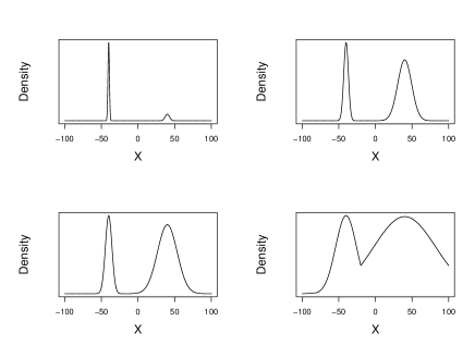
Figure 1: Power-tempered target densities of a bimodal Gaussian mixture using inverse temperature levels $\beta=\{1,0.1,0.05,0.005\}$ respectively. At the hot state it is evident that the mode centred on 40 begins to dominate the weight as $\beta\rightarrow\infty$.

Higher dimensionality makes this weight-distorting issue exponentially worse. Consider the situation with $w_{1}=w_{2}$ but $\Sigma_{1}=I_{d}$ and $\Sigma_{2}=\sigma^{2}I_{d}$ where $I_{d}$ is the $d\times d$ identity matrix. Then

$$\frac{W_{(2,\beta)}}{W_{(1,\beta)}}\approx\sigma^{d(1-\beta)},$$ (8)

so the ratio of the weights degenerates exponentially fast in the dimensionality of the problem for a fixed $\beta$. This heuristic result in (8) shows that between levels there can be a “phase-transition” in the location of probability mass, which becomes critical as dimensionality increases.

3.1 Weight Stabilised Gaussian Mixture Targets

Consider targeting a Gaussian mixture given by

$$\pi(x)\propto\sum_{j=1}^{J}w_{j}\phi(x,\mu_{j},\Sigma_{j})$$ (9)

in the (practically unrealistic) setting where the target is a Gaussian mixture with known parameters, including the weights. By only tempering the variance component of the modes, one can spread out the modes whilst preserving the component weights. We formalise this notion as follows:

Definition 1 (Weight-Stabilised Gaussian Mixture (WSGM))

For a Gaussian mixture target distribution $\pi(\cdot)$, as in (9), the weight-stabilised Gaussian mixture (WSGM) target at inverse temperature level $\beta$ is defined as

$$\pi_{\beta}^{WS}(x)\propto\sum_{j=1}^{J}w_{j}\phi\left(x,\mu_{j},\frac{\Sigma_{j}}{\beta}\right).$$ (10)

Figure 2 shows the comparison between the target distributions used when using power-based targets vs the WSGM targets for the example from Figure 1.

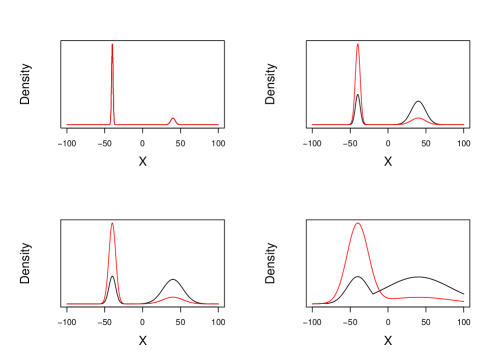
Figure 2: For a bimodal Gaussian mixture target, plots of the normalised tempered target densities generated by both powering the target (black) and the WSGM targets (red) at inverse temperature levels $\beta=\{1,0.1,0.05,0.005\}$.

Using these WSGM targets in the PT scheme can give substantially better performance than when using the standard power based targets. This is very clearly illustrated in the simulation study section below in Section 4.1. Henceforth, when the term “WSGM ST/PT Algorithm” is used it refers to the implementation of the standard ST/PT algorithm but now using the WSGM targets from (10).

3.2 Approximating the WSGM Targets

In practice, the actual target distribution would be non-Gaussian, and only approximated by a Gaussian mixture target. On the other hand, due to the improved performance gained from using the WSGM over just targeting the respective power-tempered mixture, there is motivation to approximate the WSGM in the practical setting where parameters are unknown. To this end, we present a theorem establishing useful equivalent forms of the WSGM; these alternative equivalent forms give rise to a practically applicable approximation to the WSGM.

To establish the notation, let the target be a mixture distribution given by

$$\pi(x)\propto\sum_{j=1}^{J}h_{j}(x)=\sum_{j=1}^{J}w_{j}g_{j}(x)$$ (11)

where $g_{j}(x)$ is a normalised target density. Then set

$$\pi_{\beta}(x)\propto\sum_{j=1}^{J}f_{j}(x,\beta)=\sum_{j=1}^{J}W_{(j,\beta)}\frac{[g_{j}(x)]^{\beta}}{\int[g_{j}(x)]^{\beta}dx}.$$ (12)

Then we have the following result, proved in the Appendix.

Theorem 3.1 (WSGM Equivalences)

Consider the setting of (11) and (12) where the mixture components consist of multivariate Gaussian distributions i.e. $g_{j}(x)=\phi(x;\mu_{j},\Sigma_{j})$. Then $\forall j\in 1,\ldots,J$

1. [Standard, non-weight-preserving tempering]
   If $f_{j}(x,\beta)=[h_{j}(x)]^{\beta}$ then

   $$W_{(j,\beta)}\propto w_{j}^{\beta}|\Sigma_{j}|^{\frac{1-\beta}{2}}.$$

2. [Weight-preserving tempering, version #1]
   Denoting $\nabla_{j}=\nabla\log{h_{j}(x)}$ and $\nabla_{j}^{2}=\nabla^{2}\log{h_{j}(x)}$; if $f_{j}(x,\beta)$ takes the form

   $$h_{j}(x)\exp\left\{\left(\frac{1-\beta}{2}\right)(\nabla_{j}(x))^{T}\left[\nabla^{2}_{j}(x)\right]^{-1}\nabla_{j}(x)\right\}.$$

   then $W_{(j,\beta)}\propto w_{j}$.

3. [Weight-preserving tempering, version #2]
   If

   $$f_{j}(x,\beta)=h_{j}(x)^{\beta}h_{j}(\mu_{j})^{(1-\beta)}$$

   then $W_{(j,\beta)}\propto w_{j}$.

Remark 1: In Theorem 3.1, statement (b) shows that second order gradient information of the $h_{j}$’s can be used to preserve the component weight in this setting.

Remark 2: Statement (c) extends statement (b) to no longer require the gradient information about the $h_{j}$ but simply the mode/mean point $\mu_{j}$. Essentially this shows that by appropriately rescaling according to the height of the component as the components are “powered up” then component weights are preserved in this setting.

Remark 3: A simple calculation shows that statement (c) holds for a more general mixture setting when all components of the mixture share a common distribution but different location and scale parameters.

3.3 Hessian Adjusted Tempering

The results of Theorem 3.1 are derived under the impractical setting that the components are all known and that $\pi(\cdot)$ is indeed a mixture target. One would like to exploit the results of (b) and (c) from Theorem 3.1 to aid mixing in a practical setting where the target form is unknown but may be well approximated by a mixture.

Suppose herein that the modes of the multimodal target of interest, $\pi(\cdot)$, are well separated. Thus an approximating mixture of the form given in (11) would approximately satisfy

$$\pi(x)\propto h_{M}(x)$$

where $M=\sup_{j}\left\{h_{j}(x)\right\}$. Hence it is tempting to apply a version of Theorem 3.1(b) to $\pi(\cdot)$ directly as opposed to the $h_{j}$. So at inverse temperature $\beta$, the point-wise target would be proportional to

$$\pi(x)\exp\left\{\left(\frac{1-\beta}{2}\right)(\nabla_{\pi}(x))^{T}\left[\nabla^{2}_{\pi}(x)\right]^{-1}\nabla_{\pi}(x)\right\}.$$

where $\nabla_{\pi}=\nabla\log{\pi(x)}$ and $\nabla^{2}_{\pi}=\nabla^{2}\left(\log{\pi(x)}\right)$. This only uses point-wise gradient information up to second order. At many locations in the state space, provided that $\beta$ is at a temperature level that is sufficiently cool that the tail overlap is insignificant, and if the target was indeed a Gaussian mixture then this approach would give almost exactly the same evaluations as $\pi_{\beta}(\cdot)$ from (12) in the setting of (b). However, at locations between modes when the Hessian of $\log(\pi(x))$ is positive semi-definite, this target behaves very badly, with explosion points that make it improper.

Instead, under the setting of well separated modes then one can appeal instead to the weight preserving characterisation in Theorem 3.1(c). Assume that one can assign each location in the state space to a “mode point” via some function $x\rightarrow\mu_{x,\beta}$, with a corresponding tempered target given by

$$\pi_{\beta}(x)\propto\pi(x)^{\beta}\pi(\mu_{x,\beta})^{1-\beta}.$$

Note the mode assignment function’s dependence on $\beta$. This can be understood to be necessary by appealing to Figure 2 where it is clear that the narrow mode in the WSGM target has a “basin of attraction” that expands as the temperature increases.

Definition 2 (Basic Hessian Adjusted Tempering (BHAT) Target)

For a target distribution $\pi(\cdot)$ on $\mathbb{R}^{d}$ with a corresponding “mode point assigning function” $\mu_{x,\beta}:\mathbb{R}^{d}\rightarrow\mathbb{R}^{d}$; the BHAT target at inverse temperature level $\beta\in(0,\infty)$ is defined as

$$\pi_{\beta}^{BH}(x)\propto\pi(x)^{\beta}\pi(\mu_{x,\beta})^{1-\beta}.$$ (13)

However, in this basic form there is an issue with this target distribution at hot temperatures when $\beta\rightarrow 0$. The problem is that it leaves discontinuities that can grow exponentially large and this can make the hot state temperature level mixing exponentially slow if using standard MCMC methods for the within temperature moves.

This problem can be mitigated if one assumes more knowledge about the target distribution. Suppose that the mode points are known and so there is a collection of $K$ mode points $M=\{\mu_{1},\ldots,\mu_{K}\}$. This assumption seems quite strong but in general if one cannot find mode points then this is essentially saying that one cannot find the basins of attraction and thus the desire to obtain the modal relative masses (as MCMC is trying to do) must be relatively impossible. Indeed, being able to find mode points either prior to or online in the run of the algorithm is possible e.g. Tjelmeland and Hegstad (2001), Behrens (2008) and Tawn et al. (2018). Furthermore, assume that the target, $\pi(\cdot)$, is $C^{2}$ in a neighbourhood of the $K$ mode locations and so there is an associated collection of positive definite covariance matrices $S=\{\Sigma_{1},\ldots,\Sigma_{K}\}$ where $\Sigma_{j}=-\left(\nabla^{2}\log\pi(\mu_{j})\right)^{-1}$. From this and knowing the evaluations of $\pi(\cdot)$ at the mode points then one can approximate the weights in the regions to attain a collection $\mathbf{\hat{W}}=\{\hat{w}_{1},\ldots,\hat{w}_{K}\}$ where

$$\hat{w_{j}}=\frac{\pi(\mu_{j})|\Sigma_{j}|^{1/2}}{\sum_{k=1}^{K}\pi(\mu_{k})|\Sigma_{k}|^{1/2}}$$

With $\phi(\cdot|\mu_{j},\Sigma_{j})$ denoting the pdf of a $N(\mu_{j},\Sigma_{j})$ then we define the following modal assignment function motivated by the WSGM:

Definition 3 (WSGM mode assignment function)

With collections $M$, $S$ and $\mathbf{\hat{W}}$ specified above then for a location $x\in\mathbb{R}^{d}$ and inverse temperature $\beta$ define the WSGM mode assignment function as

$$A(x,\beta)=\operatorname*{arg\,max}_{j}\left\{\hat{w}_{j}\phi\left(x|\mu_{j},\frac{\Sigma_{j}}{\beta}\right)\right\}.$$ (14)

Under the assumption that there are collections $M$, $S$ and $\mathbf{\hat{W}}$ that have either been found through prior optimisation or through an adaptive online approach we define the following:

Definition 4 (Hessian Adjusted Tempering (HAT) Target)

For a target distribution $\pi(\cdot)$ on $\mathbb{R}^{d}$ with collections $M$, $S$ and $\hat{W}$ defined above along with the associated mode assignment function given in (14), then the Hessian adjusted tempering (HAT) target is defined as

$$\pi_{\beta}^{H}(x)\propto\begin{cases}\pi(x)^{\beta}\pi(\mu_{A(x,\beta)})^{1-\beta}&\text{if $A(x,\beta)=A(x,1)$}\\ G(x,\beta)&\text{if $A(x,\beta)\neq A(x,1)$}\end{cases}$$ (15)

where with $\hat{A}:=A(x,\beta)$

$$G(x,\beta)=\frac{\pi(\mu_{\hat{A}})\left((2\pi)^{d}\Sigma_{\hat{A}}\right)^{1/2}\phi\left(x|\mu_{\hat{A}},\frac{\Sigma_{\hat{A}}}{\beta}\right)}{\beta^{d/2}}.$$

Essentially the function “$G$” specifies the target distribution when the chain’s location, $x$, is in a part of the state space where the narrower modes expand their basins of attraction as the temperature gets hotter. Both the choice of $G$ and the mode assignment function used in Definition 4 are somewhat canonical to the Gaussian mixture setting. With the same assignment function specified in Definition 3, an alternative and seemingly robust “$G$” that one could use is given by

$$G(x,\beta)=\pi(x,1,A)$$

$$+\left(\frac{2P(A(x,\beta))}{P(A(x,\beta))+P(A(x,1))}-1\right)[\pi(x,\beta,A)-\pi(x,1,A)]$$

where $\pi(x,\beta,A)=\pi(x)^{\beta}\pi(\mu_{A(x,\beta)})^{1-\beta}$ and $P(j)=\hat{w}_{j}\phi\left(x|\mu_{j},\frac{\Sigma_{j}}{\beta}\right)$.

With either of the suggested forms of the function $G$ then under the assumption that the target is continuous and bounded on $\mathbb{R}^{d}$, and that for all $\beta\in(0,\infty)$,

$$\int_{\mathcal{X}}\pi^{\beta}(x)dx<\infty\,,$$

then $\pi_{\beta}^{H}(x)$ is a well defined probability density, i.e. Definition 4 makes sense.

For a bimodal Gaussian mixture example Figure 3 compares the HAT target relative to the WSGM target; showing that the HAT targets are a very good approximation to the WSGM targets, even at the hotter temperature levels.

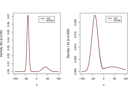
Figure 3: For the same bimodal Gaussian target from Figure 2, here is a comparison of the HAT vs WSGM targets at inverse temperatures $\beta=0.05$ and $\beta=0.005$ respectively. Note they are almost identical at the colder temperature; but they do differ slightly in the interval $(-25,10)$ at the hotter temperature where the “G” function is allowing the footprint of the narrow mode to expand.

We propose to use the HAT targets in place of the power-based targets for the tempering algorithms given in Section 2. We thus define the following algorithms, which are explored in the following sections.

Definition 5 (Hessian Adjusted Simulated Tempering (HAST) Algorithm)

The HAST algorithm is an implementation of the ST algorithm (Section 2, Algorithm 1) where the target distribution at inverse temperature level $\beta$ is given by $\pi_{\beta}^{H}(\cdot)$ from Definition 4.

Definition 6 (Hessian Adjusted (Parallel) Tempering (HAT) Algorithm)

The HAT algorithm is an implementation of the PT algorithm (Section 2, Algorithm 2) where the target distribution at inverse temperature level $\beta$ is given by $\pi_{\beta}^{H}(\cdot)$ from Definition 4.

4 Simulation Studies

4.1 WSGM Algorithm Simulation Study

We begin by comparing the performances of a ST algorithm targeting both the power-based and WSGM targets for a simple but challenging bimodal Gaussian mixture target example. The example will illustrate that the traditional ST algorithm, using power-based targets, struggles to mix effectively through the temperature levels due to a bottleneck effect caused by the lack of regional weight preservation.

The example considered is the 10-dimensional target distribution given by the bi-modal Gaussian mixture

$$\pi(x)=w_{1}\phi_{(\mu_{1},\Sigma_{1})}(x)+w_{2}\phi_{(\mu_{2},\Sigma_{2})}(x)$$ (16)

where $w_{1}=0.2$, $w_{2}=0.8$, $\mu_{1}=(-10,-10,\ldots,-10)$, $\mu_{2}=(10,10,\ldots,10)$, $\Sigma_{1}=9\mbox{\bf{I}}_{10}$ and $\Sigma_{2}=\mbox{\bf{I}}_{10}$. When power based tempering is used, then mode 1 accounts for only 20% of the mass at the cold level, but at the hotter temperature levels becomes the dominant mode containing almost all the mass.

For both runs the same geometric temperature schedule was used:

$$\Delta=\{1,\,0.32,\,0.32^{2},\,\ldots,\,0.32^{6}\}.$$

This geometric schedule is justified by Corollary 1 of Tawn and Roberts (2018), which suggests this is an optimal setup in the case of a regionally weight preserved PT setting. Indeed, this schedule induces a swap move acceptance rates around 0.22 for the WSGM algorithm; close to the suggested 0.234 optimal value.

This temperature schedule gave swap acceptance rates of approximately 0.23 between all levels of the power-based ST algorithm except for the coldest level swap where this degenerated to 0.17. That shows that the power-based ST algorithm was set up essentially optimally according to the results in Atchadé et al. (2011).

In order to ensure that the within-mode mixing isn’t influencing the temperature space mixing, a local modal independence sampler was used for the within-mode moves. This essentially means that once a mode has been found, the mixing is infinitely fast. We use the modal assignment function $\mu_{x,\beta}$ which specifies that the location $x$ is in mode 1 if $\bar{x}<0$ and in mode 2 otherwise. Then the within-move proposal distribution for a move at inverse temperature level $\beta$ is given by

$$q_{\beta}(x,y)=\phi_{\left(\mu_{1},\frac{\Sigma_{1}}{\beta}\right)}(y)\mathbbm{1}_{\bar{x}<0}+\phi_{\left(\mu_{2},\frac{\Sigma_{2}}{\beta}\right)}(y)\mathbbm{1}_{\bar{x}\geq 0},$$ (17)

where $\phi_{\mu,\Sigma}(.)$ is the density function of a Gaussian random variable with mean $\mu$ and variance matrix $\Sigma$.

Figure 4 plots a functional of the inverse temperature at each iteration of the algorithm. The functional is

$$h(\beta_{t},x_{t}):=\frac{\log\left(\frac{\beta_{t}}{\beta_{\text{min}}}\right)}{\log\left(\frac{1}{\beta_{\text{min}}}\right)}\mbox{sgn}\left(\bar{x}_{t}\right)$$ (18)

where $\mbox{sgn}(.)$ is the usual sign function and $\beta_{\text{min}}$ is the minimum of the inverse temperatures. The significance of this functional will become evident from the results of the core theoretical contributions made in this paper in Theorems 5.1 and 5.2 in Section 5. Essentially it is taking a transformation of the current inverse temperature at iteration $t$ of the Markov chain, such that when $\beta_{t}=1$ the magnitude of $h$ is 1 and when the temperature is at its hottest level, i.e. $\beta_{t}=\beta_{\text{min}}$, then $h$ is zero. Furthermore, in this example the sign of $\bar{x}_{t}$ is a reasonable proxy to identify the mode that the chain is contained in with a negative value suggesting the chain is in the mode centred on $\mu_{1}$ and $\mu_{2}$ otherwise.

Figure 4 clearly illustrates that the hot state modal weight inconsistency leads the chain down a poor trajectory since at hot temperatures nearly all the mass is in modal region 1. This results in the chain never reaching the other mode in the entire (finite) run of the algorithm. Indeed, the trace plots in Figure 4 show that the chain is effectively trapped in mode 1, which although it only has 20% of the mass in the cold state, is completely dominant at the hotter states.

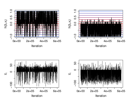
Figure 4: Top: Trace plots of the functional of the simulated tempering chains given in (18). On the left is the version using the WSGM targets, which mixes well through the temperature schedule and finds both modal regions. On the right is the version using the standard power-based targets, which fails to ever find one of the modes. Bottom: Trace plots of $\bar{x}_{t}$ in each of the cases respectively.

4.2 Simulation study for HAT

To demonstrate the capabilities of the HAT algorithm in a non-Gaussian setting where the modes exhibit skew then a five-dimensional four-mode skew-normal mixture target example is presented. Albeit a mixture, this example can be seen to give similar target distribution geometries to non-mixture settings due to the skew nature of the modes.

$$\pi(x)\propto\sum_{k=1}^{4}w_{k}\prod_{i=1}^{5}f(x_{i}|\mu_{k},\sigma_{k},\alpha)$$ (19)

where the skew normal density is given by

$$f(z|\mu,\sigma,\alpha)=\frac{2}{\sigma}\phi\left(\frac{z-\mu}{\sigma}\right)\Phi\left(\frac{\alpha(z-\mu)}{\sigma}\right)$$

and where $w_{1}=w_{2}=w_{3}=w_{4}=0.25$, $\mu_{1}=-15$, $\mu_{2}=15$, $\mu_{3}=45$, $\mu_{4}=-45$, $\sigma_{1}=1$, $\sigma_{2}=1$, $\sigma_{3}=3$, $\sigma_{4}=3$ and $\alpha=2$.

As will be seen in the forthcoming simulation results the imbalance of scales within each modal region ensures that this is a very challenging problem for the PT algorithm.

Since this target fits into the setting of Corollary 1 of Tawn and Roberts (2018) then a geometric inverse temperature schedule is approximately optimal for the HAT target in this setting. Indeed, Tawn and Roberts (2018) suggest that the geometric ratio should be tuned so that the acceptance rate for swap moves between consecutive temperatures is approximately 0.234. In this case, eight tempering levels were used to obtain effective mixing; these were geometrically spaced and given by $\{1,0.31,0.31^{2},\ldots,0.31^{7}\}$, was found to be approximately optimal and gave an average of 0.22 for the swaps between consecutive levels for the HAT algorithm.

Using this temperature schedule along with appropriately tuned RWM proposals for the within temperature moves, 10 runs of both the PT and HAT algorithms were performed. In each individual run, each temperature marginal was updated with $m=5$ RWM proposals followed by a temperature swap move proposal and this was repeated with $s=100,000$ sweeps. This results in a sample output of 600,001 of the cold state chain prior to any burn-in removal. Herein for this example denote $N=600,001$.

As expected, the scale imbalance between the modes resulted in the PT algorithm performing poorly and with significant bias in the sample output. In contrast, the HAT approach was highly successful in converging relatively rapidly to the target distribution, exhibiting far more frequent inter-modal jumps at the cold state.

Figure 5 shows one representative example of a run of the PT and HAT algorithms by plotting the first component of the five-dimensional marginal chain at the coldest target state. It illustrates the impressive inter-modal mixing of HAT across all 4 modal regions as opposed to the very sticky mixing exhibited by the PT algorithm.

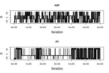
Figure 5: Two trace plots of the first marginal component cold state chain targeting the distribution in (19) using the HAT and PT algorithms respectively. Note the HAT algorithm run illustrates a chain that is performing rapid exploration between all four modes whereas the PT algorithm exhibits significant sticky patches.

Figure 6 shows the running approximation of $\mathbb{P}_{\pi}(-30<X^{1}_{i}<0)$ (which is approximately the weight of the first mode i.e. $w_{1}=0.25$) after the $k^{th}$ iteration of the cold state chains, after removing a burn-in period of 10,000 initial iterations, for the ten runs of the PT and HAT runs respectively. The approximation after iteration $k\leq N$ is given by

$$\hat{W}^{k}_{1}:=\frac{1}{k-10000}\sum_{i=10001}^{k}\mathbbm{1}_{\left(-30<X^{1}_{i}<0\right)}$$ (20)

where $X^{1}_{i}$ is the location of the first component of the five-dimensional chain at the coldest temperature level after the $i^{th}$ iteration. This figure indicates that the PT algorithm fails to provide a stable estimate for $\mathbb{P}_{\pi}(-30<X^{1}_{i}<0)$ with the running weight approximations far from stable at the end of the runs; in stark contrast the HAT algorithm exhibits very stable performance in this case. In fact the final estimates for $\hat{W}^{N}_{1}$ the are given in Table 1.

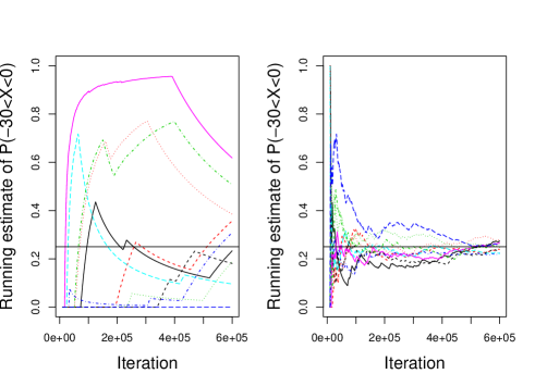
Figure 6: Running estimate of $\mathbb{P}_{\pi}(-30<X^{1}_{i}<0)$, i.e. $\hat{W}^{k}_{1}$ given in (20), for 10 runs of the PT (left) and HAT (right) algorithms. The horizontal black line at the level 0.25 represents the true probability that one aims to target in this case. In both cases a burn-in of 10,000 iterations was removed. Observe the lack of convergence of the weight estimates for the PT runs compared to the relatively impressive estimates from the HAT runs.

Table 1: The end point estimates, $\hat{W}^{N}_{1}$, of $\mathbb{P}_{\pi}(-30<X^{1}_{i}<0)$ from the 10 runs of the PT and HAT algorithms. The true value of 0.25 appears to be well approximated by HAT but not by PT.

PT	0.23	0.36	0.19	0.31	0.10	0.12	0.18
	0.39	0.51	0
HAT	0.27	0.24	0.26	0.22	0.22	0.27	0.23
	0.28	0.25	0.26

Table 2 presents the results of using the 10 runs of each algorithm in a batch-means approach to estimate the Monte Carlo variance of the estimator of $\hat{W}^{N}_{1}$. The results in Table 2 show that the Monte Carlo error is approximately a factor of 10 higher for the PT algorithm than the HAT approach.

However, it is also important to analyse this inferential gain jointly with the increase in computational cost. Table 2 also shows that the average run time for the 10 HAT runs was 451 seconds which is a little more than 2 times slower than the average run time of the PT algorithm (217 seconds) in this example. The major extra expense is due to the cost of computing the WSGM mode assignment function in (14) at both the cold and current temperature of interest at each evaluation of the HAT target. Anyhow, this is very promising since for a little more than twice the computational cost the inferential accuracy appears to be ten times better in this instance.

Table 2: Using the 10 runs of each algorithm in a batch-means approach to estimate the Monte Carlo variance of the pooled estimator $\hat{W}^{10N}_{1}$ i.e. $\text{SD}(\hat{W}^{N}_{1})$. Also displayed is the average run time (RT, measured in seconds) of a single one of the 10 repaeted runs for both methods respectively.

	$\hat{W}^{10N}_{1}$	$\hat{\text{SD}}(\hat{W}^{N}_{1})$	$\hat{\text{SD}}$($\hat{W}^{10N}_{1}$)	RT (secs)
PT	0.288	0.187	0.0593	217
HAT	0.249	0.019	0.0063	451

5 Diffusion Limit and Computational Complexity

In this section, we provide some theoretical analysis for our algorithm. We shall prove in Theorems 5.1 and 5.2 below that as the dimension goes to infinity, a simplified and speeded-up version of our weight-preserving simulated tempering algorithm (i.e., the HAST Algorithm from Definition 5, equivalent to the ST Algorithm 1 with the adjusted target from Definition 4) converges to a certain specific diffusion limit. This limit will allow us to draw some conclusions about the computational complexity of our algorithm.

5.1 Assumptions

We assume for simplicity (though see below) that our target density $\pi$ is a mixture of the form (11) with just $J=2$ modes, of weights $w_{1}=p$ and $w_{2}=1-p$ respectively, with each mixture component a special i.i.d. product $g_{j}(x)=\prod_{i=1}^{d}f_{j}(x_{i})$ as in (4). We further assume that a weight-preserving transformation (perhaps inspired by Theorem 3.1(b) or (c)) has already been done, so that

$$\pi_{\beta}(x)\ \propto \ p{[g_{1}(x)]^{\beta}\over\int[g_{1}(x)]^{\beta}dx}+(1-p){[g_{2}(x)]^{\beta}\over\int[g_{2}(x)]^{\beta}dx}$$

$$\equiv \ pg_{1}^{\beta}(x)+(1-p)g_{2}^{\beta}(x)$$

for each $\beta$. We consider a simplified version of the weight-preserving process, in which the chain always mixes immediately within each mode, but the chain can only jump between modes when at the hottest temperature $\beta_{min}$, at which point it jumps to one of the two modes with probabilities $p$ and $1-p$ respectively. Let $I$ denote the indicator of which mode the process is in, taking value $1$ or $2$.

We shall sometimes concentrate on the Exponential Power Family special case in which each of the two mixture component factors is of the form $f_{j}(x)\propto e^{-\lambda_{j}|x|^{r_{j}}}$ for some $\lambda_{j},r_{j}>0$. This includes the Gaussian case for which $r_{1}=r_{2}=2$ and $\lambda_{j}=1/\sigma_{j}^{2}$. (Note that the HAT target in (15) requires the existence of second derivatives about the mode points, corresponding to $r_{j}\geq 2$.)

As in Atchadé et al. (2011) and Roberts and Rosenthal (2014), following Predescu et al. (2004) and Kone and Kofke (2005), we assume that the inverse temperatures are given by $1=\beta_{0}^{(d)},\beta_{1}^{(d)},\ldots,\beta^{(d)}_{k(d)}\approx\beta_{\text{min}}$, with

$$\beta_{i}=\beta_{i-1}-\ell(\beta_{i-1})/d^{1/2}$$ (21)

for some fixed $C^{1}$ function $\ell$. In many cases, including the Exponential Power Family case, the optimal choice of $\ell$ is $\ell(\beta)=\beta\ell_{0}$ for a constant $\ell_{0}\doteq 2.38$.

We let $\beta_{t}^{(d)}$ be the inverse temperature at time $t$ for the $d$-dimensional process. To study weak convergence, we let $\beta^{(d)}_{N(dt)}$ be a continuous-time version of the $\beta_{t}^{(d)}$ process, speeded up by a factor of $d$, where $\{N(t)\}$ is an independent standard rate 1 Poisson process. To combine the two modes into one single process, we further augment this process by multiplying it by $-1$ when the algorithm’s state is closer to the second mode, while leaving it positive (unchanged) when state is closer to the first mode. Thus define

$$X_{t}^{(d)}=(3-2I)\,\beta^{(d)}_{N(dt)}\,.$$ (22)

5.2 Main Results

Our first diffusion limit result (proved in the Appendix), following Roberts and Rosenthal (2014), states that when we are at an inverse temperature greater than $\beta_{\text{min}}$, the inverse temperature process behaves identically to the case where there is only one mode (i.e. $J=1$).

Theorem 5.1

Assume the target $\pi$ is of the form (11), with $J=2$ modes of weights $w_{1}=p$ and $w_{2}=1-p$, with inverse weights chosen as in (21). Then up until the first time the process $X^{(d)}$ hits $\pm\beta_{\text{min}}$, as $d\to\infty$, $\{X_{t}^{(d)}\}$ converges weakly to a fixed diffusion process $X$ given by (22).

Theorem 5.1 described what happens away from $\beta_{min}$. However it says nothing about what happens at $\beta_{\text{min}}$. Moreover its statespace $[-1,-\beta_{\text{min}})\cup(\beta_{\text{min}},1]$ is not connected, and we have not even properly defined $h$ at $\pm\beta_{\text{min}}$. To resolve these issues we define

$$h(x)=\begin{cases}\int_{\beta_{\text{min}}}^{x}{1\over\ell(u)}du,&\hbox{ when }x>0\\ -\int_{\beta_{\text{min}}}^{-x}{1\over\ell(u)}du,&\hbox{ when }x<0\\ 0,&\hbox{ when }x=0\\ \end{cases}$$

and set $H_{t}=h(X_{t})$, thus making the process $H$ continuous at 0.

Remark 1

The process $H$

leaves constant densities locally invariant, ${\tilde{G}}^{*}g(v)=0$ for all $v\neq 0$ where ${\tilde{G}}^{*}$ is the adjoint of the infinitesimal generator of $H$, as will be shown in the Appendix. This suggests that the density of the invariant distribution of $H$ (if it exists) should be piecewise uniform, i.e. it should be constant for $v>0$ and also constant for $v<0$ though these two constants might not be equal.

To make further progress, we require a proportionality condition. Namely, we assume that the quantities corresponding to $I(\beta)=\text{Var}_{\pi^{\beta}}\big{(}\log f(x)\big{)}$ are proportional to each other in the two modes. More precisely, we extend the definition of $I$ to $I(\beta)=\text{Var}_{x\sim f_{1}^{\beta}}(\log f_{1}(x))$ for $\beta>0$ (corresponding to the first mode), and $I(\beta)=\text{Var}_{x\sim f_{2}^{|\beta|}}(\log f_{2}(x))$ for $\beta<0$ (corresponding to the second mode), and assume there is a fixed function $I_{0}:\mathbb{R}_{+}\to\mathbb{R}_{+}$ and positive constants $r_{1}$ and $r_{2}$ such that we have $I(\beta)=I_{0}(\beta)/r_{1}$ for $\beta>0$ (in the first mode), while $I(\beta)=I_{0}(|\beta|)/r_{2}$ for $\beta<0$ (in the second mode). For example, it follows from Section 2.4 of Atchadé et al. (2011) that in the Exponential Power Family case, $I(\beta)=1/r_{1}\beta^{2}$ for $\beta>0$ and $I(\beta)=1/r_{2}\beta^{2}$ for $\beta<0$, so that this proportionality condition holds in that case.

Corresponding to this, we choose the inverse temperature spacing function as follows (following Atchadé et al. (2011) and Roberts and Rosenthal (2014)):

$$\ell(\beta)\ =\ I_{0}^{-1/2}(\beta)\,\ell_{0}$$ (23)

for some fixed constant $\ell_{0}>0$.

To state our next result, we require the notion of skew Brownian motion, a generalisation of usual Brownian motion. Informally, this is a process that behaves just like a Brownian motion, except that the sign of each excursion from 0 is chosen using an independent Bernoulli random variable; for further details and constructions and discussion see e.g. Lejay (2006). We also require the function

$$z(h)\ =\ h\,\left[2\,\Phi\left({-\ell_{0}\over 2\sqrt{r(h)}}\right)\right]^{-1/2}\,.$$

where $r(h)=r_{1}$ for $h>0$ and $r(h)=r_{2}$ for $h<0$. We then have the following result (also proved in the Appendix).

Theorem 5.2

Under the set-up and assumptions of Theorem 5.1, assuming the above proportionality condition and the choice (23), then as $d\to\infty$, the process $\{X_{t}^{(d)}\}$ converges weakly in the Skorokhod topology to a limit process $X$. Furthermore, the limit process has the property that if

$$Z_{t}=z\big{(}h(X_{t})\big{)}\,,$$

then $Z$ is skew Brownian motion $B^{*}_{t}$ with reflection at

$$(3-2i)\left[2\,\Phi\left({-\ell_{0}\over 2\sqrt{r_{i}}}\right)\right]^{-1/2}\int_{\beta_{\text{min}}}^{1}{1\over\ell(u)}du,\ \ \ i=1,2\ .$$ (24)

Remark 2

It follows from the proof of Theorem 5.2 that the specific version of skew Brownian motion $B^{*}_{t}$ that arises in the limit is one with excursion weights proportional to

$$a=p\left[2\Phi\left({-\ell_{0}\over 2\sqrt{r_{1}}}\right)\right]^{1/2}\text{and\leavevmode\nobreak\ }b=(1-p)\left[2\Phi\left({-\ell_{0}\over 2\sqrt{r_{2}}}\right)\right]^{1/2}.$$

That means that the stationary density for $B^{*}_{t}$ on the positive and negative values is proportional to $a$ and $b$ respectively. This might seem surprising since the limiting weights of the modes should be equal to $p$ and $1-p$, not proportional to $a$ and $b$ (unless $r_{1}=r_{2}$). The explanation is that the lengths of the positive and negative parts of the domain are given by $\left[2\,\Phi\left({-\ell_{0}\over 2\sqrt{r_{1}}}\right)\right]^{1/2}$ and $\left[2\,\Phi\left({-\ell_{0}\over 2\sqrt{r_{2}}}\right)\right]^{1/2}$ respectively. Hence, the total stationary mass of the positive and negative parts – and hence also the limiting modes weights – are still $p$ and $1-p$ as they should be.

5.3 Complexity Order

Theorems 5.1 and 5.2 have implications for the computational complexity of our algorithm.

In Theorem 5.1, the limiting diffusion process $H_{t}$ is a fixed process, not depending on dimension except through the value of $\beta_{\text{min}}$. It follows that if $\beta_{\text{min}}$ is kept fixed, then $H_{t}$ reaches 0 (and hence mixes modes) in time $O(1)$. Since $H_{t}$ is derived (via $X_{t}$) from the $\beta_{t}$ process speeded up by a factor of $d$, it thus follows that for fixed $\beta_{\text{min}}$, $\beta_{t}$ reaches $\beta_{\text{min}}$ (and hence mixes modes) in time $O(d)$. So, if $\beta_{\text{min}}$ is kept fixed, then the mixing time of the weight-preserving tempering algorithm is $O(d)$, which is very fast. However, this does not take into account the dependence on $\beta_{\text{min}}$, which might also change as a function of $d$.

Theorem 5.2 allows for control of the dependence of mixing time on the values of $\beta_{\text{min}}$. The limiting skew Brownian motion process $B^{*}_{t}$ is a fixed process, not depending on dimension nor on $\beta_{\text{min}}$, with range given by the reflection points in (24). It follows that $Z_{t}$ reaches 0 (and hence mixes modes) in time of order the square of the total length of the interval, i.e. of order

$$\left(\sum_{i=1}^{2}\left[2\,\Phi\left({-\ell_{0}\over 2\sqrt{r_{i}}}\right)\right]^{-1/2}\int_{\beta_{min}}^{1}{1\over\ell(u)}du\right)^{2}$$

In the Exponential Power Family case, this is easily computed to be $O\big{(}d\,[\log\beta_{\text{min}}]^{2}\big{)}$.

This raises the question of how large $\beta_{\text{min}}$ needs to be, as a function of dimension $d$. If the proposal scaling is optimal for within each mode at the cold temperature, then the proposal scaling is $O(d^{-1/2})$. Then, at an inverse temperature $\beta$, the proposal scaling is $O((\beta d)^{-1/2})$. Hence, at an inverse temperature $\beta$, the probability of jumping from one mode to the other (a distance $O(\sqrt{d})$ away) is roughly of order $e^{-\beta d^{2}}$. This is exponentially small unless $\beta=O(1/d^{2})$. This indicates that, for our algorithm to perform well, we need to choose $\beta_{\text{min}}=O(1/d^{2})$. With this choice, the mixing time order becomes

$$\left(\sum_{i=1}^{2}\left[2\,\Phi\left({-\ell_{0}\over 2\sqrt{r_{i}}}\right)\right]^{-1/2}\int_{1/d^{2}}^{1}{1\over\ell(u)}du\right)^{2}$$

In the Exponential Power Family case, this corresponds to $O\big{(}d\,[\log d]^{2}\big{)}$. That is, for the inverse temperature process to hit $\beta_{\text{min}}$ and hence mix modes, takes $O\big{(}d\,[\log d]^{2}\big{)}$ iterations. This is a fairly modest complexity order, and compares very favourably to the exponentially large convergence times which arise for traditional simulated tempering as discussed in Subsection 2.2.

5.4 More than Two Modes

Finally, we note that for simplicity, the above analysis was all done for just two modes. However, a similar analysis works more generally. Indeed, suppose now that we have $k$ modes, of general weights $p_{1},p_{2},\ldots,p_{k}\geq 0$ with $\sum_{i}p_{i}=1$. Then when $\beta$ gets to $\beta_{\text{min}}$, the process chooses one of the $k$ modes with probability $p_{i}$. This corresponds to $\{Y_{t}\}$ being replaced by a Brownian motion not on $[-1,1]$, but rather on a “star” shape with $k$ different length-1 line segments all meeting at the origin (corresponding, in the original scaling, to $\beta_{\text{min}}$), where each time the Brownian motion hits the origin it chooses one of the $k$ line segments with probability $p_{i}$ each. This process is called Walsh’s Brownian motion, see e.g. Barlow et al. (1989). (The case $k=2$ but $p_{1}\not=1/2$ corresponds to skew Brownian motion as above.) For this generalised process, a theorem similar to Theorem 5.1 can be then stated and proved by similar methods, leading to the same complexity bound of $O\big{(}d\,[\log d]^{2}\big{)}$ iterations in the multimodal case as well.

6 Conclusion and Further Work

This article has introduced the HAT algorithm to mitigate the lack of regional weight preservation in standard power-based tempered targets. Our simulation studies show promising mixing results, and our theorems indicate the mixing times can become polynomial rather than exponential functions of the dimension $d$, and indeed of time $O(d[\log d]^{2})$ under appropriate assumptions.

Various questions remain to make our HAT approach more practically applicable. The “modal assignment function” needs to be specified in an appropriate way, and more exploration into the robustness of the current assignment mechanism is needed to understand its performance on heavier and lighter tailed distributions. The suggested HAT target assumes knowledge of the mode points which typically one will not have to begin with and one would rely on effective optimisation methods to seek these out either during or prior to the run of the algorithm. Indeed, this has been partially explored by the authors in Tawn et al. (2018). The performance of HAT is heavily reliant on the mixing at the hottest temperature level; the use of RWM here can be problematic for HAT where the mode heights of the disperse modes can be far lower than the narrower modes. As such more advanced sampling schemes such as discretised tempered Langevin could give accelerated mixing at the hot state; the effects of which would be transferred to an improvement in the mixing at the coldest state.

In the theoretical analysis of Section 5, the spacing between consecutive inverse-temperature levels was taken to be $O(d^{-1/2})$ to induce a non trivial diffusion limit. However, this result required strong assumptions. Accompanying work in Tawn and Roberts (2018) suggests that for the HAT algorithm under more general conditions, the consecutive optimal spacing should still be $O(d^{-1/2})$, with an associated optimal acceptance rate in the interval $[0,0.234]$.

7 Appendix

In this Appendix, we prove the theorems stated in the paper.

7.1 Proof of Theorem 3.1

Herein, assume the mixture distribution setting of (11) and (12) where the mixture components consist of multivariate Gaussian distributions i.e. $g_{j}(x)=\phi(x;\mu_{j},\Sigma_{j})$. We prove each of the three parts of Theorem 3.1 in turn.

Proof (Proof of Theorem 3.1(a))

Recall that $h_{j}(x)=w_{j}\phi(x;\mu_{j},\Sigma_{j})$ where $\exists C\in\mathbb{R}$ such that $C\sum_{j=1}^{J}w_{j}=1$. Hence, taking $f_{j}(x,\beta)=[h_{j}(x)]^{\beta}$ gives

$$f_{j}(x,\beta) = w_{j}^{\beta}\phi(x;\mu_{j},\Sigma_{j})^{\beta}$$

$$= w_{j}^{\beta}\left[\frac{\left((2\pi)^{d}|\Sigma_{j}|\right)^{\frac{1-\beta}{2}}}{\beta^{d/2}}\right]\phi\left(x;\mu_{j},\frac{\Sigma_{j}}{\beta}\right)$$

$$\propto w_{j}^{\beta}|\Sigma_{j}|^{\frac{1-\beta}{2}}\phi\left(x;\mu_{j},\frac{\Sigma_{j}}{\beta}\right)$$

Proof (Proof of Theorem 3.1(b))

Recall the result of Theorem 3.1(a). To adjust for the weight discrepancy from the cold state target a multiplicative adjustment factor, $\alpha_{j}(x)$ is used such that

$$f_{j}(x,\beta)=h_{j}(x)^{\beta}\alpha_{j}(x,\beta)$$

where $\alpha_{j}(x,\beta)=\left(w_{j}^{\beta}|\Sigma_{j}|^{\frac{1-\beta}{2}}\right)^{-1}$. An identical argument to Theorem 3.1(a) shows that this immediately gives $W_{(j,\beta)}\propto w_{j}$.

In a Gaussian setting, up to a proportionality constant

$$w_{j}\propto h_{j}(x)\left[(2\pi)^{\frac{d}{2}}|\Sigma_{j}|^{\frac{1}{2}}\exp\left\{\frac{1}{2}(x-\mu_{j})^{T}\Sigma_{j}^{-1}(x-\mu_{j})\right\}\right]$$ (25)

and at any point $x\in\mathbb{R}^{d}$

$$\nabla\log{h_{j}(x)} = -\Sigma_{j}^{-1}(x-\mu_{j})$$ (26)

$$\nabla^{2}\log{h_{j}(x)} = -\Sigma_{j}^{-1}.$$ (27)

Substituting these gradient terms (26) and (27) into (25) and then using this form of (25) to create the adjustment factor $\alpha_{j}(x,\beta)=\left(w_{j}^{\beta}|\Sigma_{j}|^{\frac{1-\beta}{2}}\right)^{-1}$ completes the proof.

Proof (Proof of Theorem 3.1(c))

Since $h_{j}(x)=w_{j}\phi(x;\mu_{j},\Sigma_{j})$ then

$$f_{j}(x,\beta) = h_{j}(x)^{\beta}h_{j}(\mu_{j})^{(1-\beta)}$$

$$= w_{j}\phi(x;\mu_{j},\Sigma_{j})^{\beta}\phi(\mu_{j};\mu_{j},\Sigma_{j})^{(1-\beta)}$$

$$= \frac{w_{j}}{\beta^{d/2}}\phi\left(x;\mu_{j},\frac{\Sigma_{j}}{\beta}\right)$$

and so $W_{(j,\beta)}\propto w_{j}$.

Remark 3

It is possible to extend the weight adjusted target result of Theorem 3.1(c) to a setting where the target consists of a mixture of a general but common distribution, with each component having a different shape and scale factor; we plan to pursue this result elsewhere.

Since mixing between modes is only possible at $\beta_{min}$, the dynamics will be identical to the single mode case ($J=1$) as covered in Roberts and Rosenthal (2014). It therefore follows directly from Theorem 6 of Roberts and Rosenthal (2014) that as $d\to\infty$, the process $\{X_{t}\}$ converges weakly, at least on $X_{t}>0$, to a diffusion limit $\{X_{t}\}_{t\geq 0}$ satisfying

$$dX_{t} = \left[2\ell^{2}(X_{t})\,\Phi\left({-\ell(X_{t})I^{1/2}(X_{t})\over 2}\right)\right]^{1/2}dB_{t}\big{.}$$

$$+\,\Bigg{[}\ell(X_{t})\,\ell^{\prime}(X_{t})\ \Phi\left({-I^{1/2}(X_{t})\ell(X_{t})\over 2}\right)\big{.}$$

$$-\,\ell^{2}(X_{t})\left({\ell(X_{t})I^{1/2}(X_{t})\over 2}\right)^{\prime}\phi\left({-I^{1/2}(X_{t})\ell(X_{t})\over 2}\right)\Bigg{]}dt\,,$$

where $I(\beta)=\text{Var}_{x\sim f_{1}^{\beta}}(\log f_{1}(x))$. If we extend the definition of $I$ to $I(\beta)=\text{Var}_{x\sim f_{1}^{\beta}}(\log f_{1}(x))$ for $\beta>0$, and $I(\beta)=\text{Var}_{x\sim f_{2}^{|\beta|}}(\log f_{2}(x))$ for $\beta<0$, so that positive values correspond to the first mode while negative values correspond to the second mode, then (7.1) also holds for $X_{t}<0$, except with the sign of the drift reversed.

7.2 Proof of Remark 1

We note that for $x>0$ (with exactly analogous results for $x<0$), $h^{\prime}(x)=\ell(x)^{-1}$, and $h^{\prime\prime}(x)=-\ell^{\prime}(x)\ell(x)^{-2}$. So, if we set $H_{t}=h(X_{t})$, then we compute by Ito’s Formula that

$$dH_{t} = h^{\prime}(X_{t})dX_{t}+\frac{1}{2}h^{\prime\prime}(X_{t})d\langle X\rangle_{t}$$

$$= \ell(X_{t})^{-1}dX_{t}-\frac{1}{2}\ell^{\prime}(X_{t})\ell(X_{t})^{-2}d\langle X\rangle_{t}$$

$$= \ell(X_{t})^{-1}\left[2\ell^{2}(X_{t})\Phi\left(\frac{-\ell(X_{t})I^{1/2}(X_{t})}{2}\right)\right]^{1/2}dB_{t}$$

$$+\ell(X_{t})^{-1}\Bigg{[}\ell(X_{t})\ell^{\prime}(X_{t})\Phi\left(\frac{-I^{1/2}(X_{t})\ell(X_{t})}{2}\right)$$

$$-\ell^{2}(X_{t})\left(\frac{\ell(X_{t})I^{1/2}(X_{t})}{2}\right)^{\prime}\phi\left(\frac{-I^{1/2}(X_{t})\ell(X_{t})}{2}\right)\Bigg{]}dt$$

$$-\frac{1}{2}\ell^{\prime}(X_{t})\ell(X_{t})^{-2}\left[2\ell^{2}(X_{t})\Phi\left(\frac{-\ell(X_{t})I^{1/2}(X_{t})}{2}\right)\right]dt$$

$$= \left[2\Phi\left(\frac{-\ell(X_{t})I^{1/2}(X_{t})}{2}\right)\right]^{1/2}dB_{t}$$

$$+\Bigg{[}\ell^{\prime}(X_{t})\ \Phi\left(\frac{-I^{1/2}(X_{t})\ell(X_{t})}{2}\right)$$

$$-\ell(X_{t})\left(\frac{\ell(X_{t})I^{1/2}(X_{t})}{2}\right)^{\prime}\phi\left(\frac{-I^{1/2}(X_{t})\ell(X_{t})}{2}\right)\Bigg{]}dt$$

$$\leavevmode\nobreak\ \leavevmode\nobreak\ \leavevmode\nobreak\ \leavevmode\nobreak\ -\frac{1}{2}\ell^{\prime}(X_{t})\left[2\,\Phi\left({-\ell(X_{t})I^{1/2}(X_{t})\over 2}\right)\right]dt$$

$$= \left[2\,\Phi\left({-\ell(X_{t})I^{1/2}(X_{t})\over 2}\right)\right]^{1/2}dB_{t}$$ (28)

$$-\,\ell(X_{t})\left({\ell(X_{t})I^{1/2}(X_{t})\over 2}\right)^{\prime}\phi\left({-I^{1/2}(X_{t})\ell(X_{t})\over 2}\right)dt$$

$$= \left[2\,\Phi\left({-\ell(X_{t})I^{1/2}(X_{t})\over 2}\right)\right]^{1/2}dB_{t}$$

$$+\ \ell(X_{t})\,\Bigg{[}\Phi\left({-I^{1/2}(X_{t})\ell(X_{t})\over 2}\right)\Bigg{]}^{\prime}dt$$

Re-writing everything in terms of $H_{t}=h(X_{t})$, this becomes

$$dH_{t}\ =\ \left[2\,\Phi\left({-\ell(h^{-1}(H_{t}))I^{1/2}(h^{-1}(H_{t}))\over 2}\right)\right]^{1/2}dB_{t}$$

$$+\,\ell(h^{-1}(H_{t}))\,\Bigg{[}\Phi\left({-I^{1/2}(h^{-1}(H_{t}))\ell(h^{-1}(H_{t}))\over 2}\right)\Bigg{]}^{\prime}dt\,.$$ (29)

Now, in general, a diffusion of the form $dH_{t}=\sigma(H_{t})dB_{t}+\mu(H_{t})dt$ has locally invariant distribution $\pi$ provided that $\frac{1}{2}(\log\pi)^{\prime}\sigma^{2}+\sigma\sigma^{\prime}=\mu$. In particular, it has a uniform locally ivariant distribution , i.e. with $\pi$ constant, provided that $\mu=\sigma\sigma^{\prime}$, i.e. that $2\mu=(\sigma^{2})^{\prime}$. In this specific case, we verify that

$$(\sigma^{2})^{\prime}\ =\ {d\over dH}\left[2\,\Phi\left({-\ell(h^{-1}(H))I^{1/2}(h^{-1}(H))\over 2}\right)\right]$$

$$\ =\ \left({dH\over dX}\right)^{-1}{d\over dX}\left[2\,\Phi\left({-\ell(X)I^{1/2}(X)\over 2}\right)\right]$$

$$\ =\ \left(\ell(X)^{-1}\right)^{-1}\left[2\,\Phi\left({-\ell(X)I^{1/2}(X)\over 2}\right)\right]^{\prime}$$

which is indeed equal to $2\mu$ since in the above equation

$$\mu\ =\ \ell(X)\,\Bigg{[}\Phi\left({-I^{1/2}(X)\ell(X)\over 2}\right)\Bigg{]}^{\prime}\,.$$

Therefore $H$ leaves constant densities locally invariant.

7.3 Proof of Theorem 5.2

We now assume that $I(\beta)=I_{0}(\beta)/r_{1}$ for $\beta>0$, while $I(\beta)=I_{0}(|\beta|)/r_{2}$ for $\beta<0$, and that $\ell(\beta)=I_{0}^{-1/2}(\beta)\,\ell_{0}$. This makes $\leavevmode\nobreak\ \ell(x)I^{1/2}(x)=\ell_{0}/\sqrt{r_{1}}\leavevmode\nobreak\$ for $x>0$, and $\ell(x)I^{1/2}(x)=\ell_{0}/\sqrt{r_{2}}$ for $x<0$. In either case, $\ell(x)I^{1/2}(x)$ is constant, i.e. has derivative zero. That in turn collapses (28), at least for $H_{t}\not=0$, into the simpler

$$dH_{t}\ =\ \left[2\,\Phi\left({-\ell_{0}\over 2\sqrt{r(H_{t})}}\right)\right]^{1/2}dB_{t}\,,$$

where $r(H)=r_{1}$ for $H>0$ and $r(H)=r_{2}$ for $H<0$.

Finally, we set

$$Z_{t}\ =\ H_{t}\,\left[2\,\Phi\left({-\ell_{0}\over 2\sqrt{r(H_{t})}}\right)\right]^{-1/2}.$$

That is, $Z_{t}$ is a version of $H_{t}$ which is stretched by a piecewise linear spatial function, which is linear on each of the positive and negative values respectively. It then follows immediately from the above that $dZ_{t}=dB_{t}$, i.e. that $Z_{t}$ behaves like Brownian motion on each of its two branches (positive and negative). It remains only to prove that at $Z_{t}=0$, the convergence still holds.

We complete the proof similarly to previous proofs of diffusion limits of MCMC algorithms (e.g. Roberts et al. (1997); Roberts and Rosenthal (1998); Bédard and Rosenthal (2008)), following the approach indicated in Chapter 4 of Ethier and Kurtz (1986) (in particular Corollary 8.7 of that chapter), by proving that the generator $G^{(d)}$ of the original process under these combined transformations (i.e., jumping according to a rate $d$ Poisson process, then transformed by the $h$ function, and then stretched by the piecewise linear function) converges uniformly to the generator $G^{*}$ of skew Brownian motion, when applied to a core of functionals.

Let $z_{\text{max}}=\int_{\beta_{\text{min}}}^{1}\ell^{-1}(u)\times 2\Phi(-\ell_{0}/(2\sqrt{r_{1}})$ and let $z_{\text{min}}=-\int_{\beta_{\text{min}}}^{1}\ell^{-1}(u)\times 2\Phi(-\ell_{0}/(2\sqrt{r_{2}})$. We let $\mathcal{D}$ be the set of all functions $f:[-z_{\text{min}},z_{\text{max}}]\to\mathbb{R}$ which are continuous and twice-continuously-differentiable on $[z_{\text{min}},0]$ and also on $[0,z_{\text{max}}]$, with matching one-sided second derivatives $f^{\prime\prime+}(0)=f^{\prime\prime-}(0)$, and skewed one-sided first derivatives satisfying $af^{\prime+}(0)=bf^{\prime-}(0)$ where $a=p\left[2\,\Phi\left({-\ell_{0}\over 2\sqrt{r_{1}}}\right)\right]^{1/2}$ and $b=(1-p)\left[2\,\Phi\left({-\ell_{0}\over 2\sqrt{r_{2}}}\right)\right]^{1/2}$. Finally we require that $f^{\prime}(z_{\text{max}})=f^{\prime}(z_{\text{min}})=0$ to describe the reflecting boundaries at the endpoints. Thus, $C^{2}$ functions are not contained in $\mathcal{D}$ due the enforced discontinuity of the first derivative at $0$, but e.g. $f\in\mathcal{D}$ if $f(x)=x^{2}+ax\mathbbm{1}_{x<0}+bx\mathbbm{1}_{x>0}$. In particular, $\mathcal{D}$ is dense (in the sup norm) in the set of all $C^{2}[z_{\text{min}},z_{\text{max}}]$ functions, so in the language of Ethier and Kurtz (1986), $\mathcal{D}$ serves as a core of functions for which it suffices to prove that the generators converge. Furthermore, it follows from e.g. Liggett (2010) and Exercise 1.23 of Chapter VII of Revuz and Yor (2004)) that the generator of skew Brownian motion (with excursion weights proportional to $a$ and $b$ respectively) satisfies that $G^{*}f(x)=\frac{1}{2}f^{\prime\prime}(0)$ for all $f\in\mathcal{D}$, using the convention that $f^{\prime\prime}(0)$ represents the common value $f^{\prime\prime+}(0)=f^{\prime\prime-}(0)$.

Now, it follows from the previous discussion that for any fixed $f\in\mathcal{D}$,

$$\lim_{d\to\infty}\sup_{z\in\left[z_{\text{min}},z_{\text{max}}\right]\setminus\{0\}}|G^{(d)}f(z)-G^{*}f(z)|=0\,.$$ (30)

That is, the generators do converge uniformly to the $G^{*}$, as required, at least for $z\not=0$, i.e. avoiding the mode-hopping value $\beta_{\text{min}}$. To complete the proof, it suffices to prove that (30) also holds at $z=0$, i.e. to prove:

Lemma 1

We have that:

$$\lim_{d\to\infty}G^{(d)}f(0)\ =\ G^{*}f(0)\ =\ \,\frac{1}{2}\,f^{\prime\prime}(0)\,.$$

Proof

Note first that if the original inverse-temperature process proposes to move the inverse-temperature from $\beta_{\text{min}}$ to $\beta_{\text{min}}+\ell(\beta_{\text{min}})d^{-1/2}$, then the $H_{t}$ process proposes to move from $0$ to $\pm d^{-1/2}$, and the $Z_{t}$ process proposes to move from $0$ to $\pm d^{-1/2}\left[2\,\Phi\left(\frac{-\ell_{0}}{2\sqrt{r(\pm)}}\right)\right]^{-1/2}$. Furthermore, the $Z_{t}$ process, like the $X_{t}$ process, is sped up by a factor of $d$, which multiplies its generator by $d$. Hence, we conclude that

$$G^{(d)}f(0)\ =\ d\left(p\alpha_{+}\left[f\left(d^{-1/2}\left[2\,\Phi\left({-\ell_{0}\over 2\sqrt{r_{1}}}\right)\right]^{-1/2}\right)-f(0)\right]\right.$$

$$\,+\,\left.(1-p)\alpha_{-}\left[f\left(d^{-1/2}\left[2\,\Phi\left({-\ell_{0}\over 2\sqrt{r_{2}}}\right)\right]^{-1/2}\right)-f(0)\right]\right)\,,$$

where $\alpha_{+}$ is the acceptance probability for the original process to accept a proposal to increase the inverse-temperature from $\beta_{\text{min}}$ to $\beta_{\text{min}}+\ell(\beta_{\text{min}})d^{-1/2}$ in mode 1, and $\alpha_{-}$ is the acceptance probability for the same proposal in mode 2.

Next, note that the process $Z_{t}$ has expected squared jumping distance equal to the square of its volatility, which is just equal to 1. On the other hand, the expected squared jumping distance must be equal to the squared distance of its proposed move times the acceptance probability. Hence, in mode 1, we must have

$$1\ =\ \left(\left[2\,\Phi\left({-\ell_{0}\over 2\sqrt{r_{1}}}\right)\right]^{-1/2}\right)^{2}\alpha_{+}$$

whence

$$\alpha_{+}\ =\ 2\,\Phi\left({-\ell_{0}\over 2\sqrt{r_{1}}}\right)$$

and similarly

$$\alpha_{-}\ =\ 2\,\Phi\left({-\ell_{0}\over 2\sqrt{r_{2}}}\right)\,.$$

Then, taking a Taylor series expansion, we obtain that for $f\in\mathcal{D}$,

$$G^{(d)}f(0) = d\Bigg{(}p\alpha_{+}\left[f\left(d^{-1/2}\left[2\Phi\left({-\ell_{0}\over 2\sqrt{r_{1}}}\right)\right]^{-1/2}\right)-f(0)\right]$$

$$+(1-p)\alpha_{-}\left[f\left(-d^{-1/2}\left[2\,\Phi\left({-\ell_{0}\over 2\sqrt{r_{2}}}\right)\right]^{-1/2}\right)-f(0)\right]\Bigg{)}$$

$$= dp\left[2\,\Phi\left({-\ell_{0}\over 2\sqrt{r_{1}}}\right)\right]\left(d^{-1/2}\left[2\,\Phi\left({-\ell_{0}\over 2\sqrt{r_{1}}}\right)\right]^{-1/2}\right)f^{\prime+}(0)$$

$$-\ \frac{1}{2}dp\left[2\,\Phi\left({-\ell_{0}\over 2\sqrt{r_{1}}}\right)\right]\left(d^{-1/2}\left[2\,\Phi\left({-\ell_{0}\over 2\sqrt{r_{1}}}\right)\right]^{-1/2}\right)^{2}f^{\prime\prime+}(0)$$

$$+O(dp\alpha_{+}d^{-3/2})$$

$$+ \Bigg{[}d(1-p)\left[2\,\Phi\left({-\ell_{0}\over 2\sqrt{r_{2}}}\right)\right]$$

$$\times\left(d^{-1/2}\left[2\,\Phi\left({-\ell_{0}\over 2\sqrt{r_{2}}}\right)\right]^{-1/2}\right)f^{\prime-}(0)\Bigg{]}$$

$$+ \Bigg{[}\frac{1}{2}d(1-p)\left[2\,\Phi\left({-\ell_{0}\over 2\sqrt{r_{2}}}\right)\right]$$

$$\times\left(d^{-1/2}\left[2\,\Phi\left({-\ell_{0}\over 2\sqrt{r_{2}}}\right)\right]^{-1/2}\right)^{2}f^{\prime\prime-}(0)\Bigg{]}$$

$$+ O(dp\alpha_{+}d^{-3/2})$$

$$= d^{1/2}p\left[2\,\Phi\left(\frac{-\ell_{0}}{2\sqrt{r_{1}}}\right)\right]^{1/2}f^{\prime+}(0)+\frac{1}{2}pf^{\prime\prime+}(0)$$

$$-d^{1/2}(1-p)\left[2\,\Phi\left(\frac{-\ell_{0}}{2\sqrt{r_{2}}}\right)\right]^{1/2}f^{\prime-}(0)$$

$$+\frac{1}{2}(1-p)f^{\prime\prime-}(0)+O(d^{-1/2}).$$

Then, by definition of $f\in\mathcal{D}$, the terms involving $f^{\prime+}(0)$ and $f^{\prime-}(0)$ cancel, and the terms involving $f^{\prime\prime+}(0)$ and $f^{\prime\prime-}(0)$ combine. Recalling the convention $f^{\prime\prime}(0)=f^{\prime\prime+}(0)=f^{\prime\prime-}(0)$, we obtain finally that

$$G^{(d)}f(0)\ =\ \frac{1}{2}f^{\prime\prime}(0)+O(d^{-1/2})$$

so that

$$\lim_{d\to\infty}G^{(d)}f(0)\ =\ \frac{1}{2}f^{\prime\prime}(0)\ =\ G^{*}f(0)$$

as claimed.

References

- Atchadé and Liu (2004) Atchadé YF, Liu JS (2004) The Wang-Landau algorithm for Monte Carlo computation in general state spaces. Statistica Sinica 20:209–33
- Atchadé et al. (2011) Atchadé YF, Roberts GO, Rosenthal JS (2011) Towards optimal scaling of Metropolis-coupled Markov chain Monte Carlo. Statistics and Computing 21(4):555–568
- Barlow et al. (1989) Barlow MT, Pitman J, Yor M (1989) On Walsh’s Brownian motions. Séminaire de probabilités (Strasbourg) 23:275–293
- Bédard and Rosenthal (2008) Bédard M, Rosenthal JS (2008) Optimal scaling of Metropolis algorithms: Heading toward general target distributions. The Canadian Journal of Statistics 36:483–503
- Behrens (2008) Behrens GR (2008) Mode Jumping in MCMC. PhD thesis, University of Bath
- Bhatnagar and Randall (2016) Bhatnagar N, Randall D (2016) Simulated tempering and swapping on mean-field models. Journal of Statistical Physics 164(3):495–530
- Ethier and Kurtz (1986) Ethier SN, Kurtz TG (1986) Markov Processes: Characterization and Convergence. John Wiley & Sons
- Geyer (1991) Geyer CJ (1991) Markov chain Monte Carlo maximum likelihood. Computing Science and Statistics 23:156–163
- Kone and Kofke (2005) Kone A, Kofke DA (2005) Selection of Temperature Intervals for Parallel-Tempering Simulations. The Journal of Chemical Physics 122(20):206101
- Kou et al. (2006) Kou S, Zhou Q, Wong WH (2006) Equi-energy sampler with applications in statistical inference and statistical mechanics. The Annals of Statistics pp 1581–1619
- Lejay (2006) Lejay A (2006) On the constructions of the skew Brownian motion. Probability Surveys 3:413–466
- Liggett (2010) Liggett TM (2010) Continuous Time Markov Processes: An Introduction. American Mathematical Society
- Marinari and Parisi (1992) Marinari E, Parisi G (1992) Simulated tempering: a new Monte Carlo scheme. EPL (Europhysics Letters) 19(6):451
- Miasojedow et al. (2013) Miasojedow B, Moulines E, Vihola M (2013) An adaptive parallel tempering algorithm. Journal of Computational and Graphical Statistics 22(3):649–664
- Neal (1996) Neal RM (1996) Sampling from multimodal distributions using tempered transitions. Statistics and Computing 6(4):353–366
- Nemeth et al. (2017) Nemeth C, Lindsten F, Filippone M, Hensman J (2017) Pseudo-extended Markov Chain Monte Carlo. ArXiv e-prints 1708.05239
- Predescu et al. (2004) Predescu C, Predescu M, Ciobanu CV (2004) The Incomplete Beta Function Law for Parallel Tempering Sampling of Classical Canonical Systems. The Journal of Chemical Physics 120(9):4119–4128
- Revuz and Yor (2004) Revuz D, Yor M (2004) Continuous Martingales and Brownian Motion, 3rd edn. Springer
- Robbins and Monro (1951) Robbins H, Monro S (1951) A stochastic approximation method. The Annals of Mathematical Statistics pp 400–407
- Roberts and Rosenthal (1998) Roberts GO, Rosenthal JS (1998) Optimal scaling of discrete approximations to Langevin diffusions. Journal of the Royal Statistical Society: Series B (Statistical Methodology) 60(1):255–268
- Roberts and Rosenthal (2001) Roberts GO, Rosenthal JS (2001) Optimal scaling for various Metropolis-Hastings algorithms. Statistical Science 16(4):351–367
- Roberts and Rosenthal (2009) Roberts GO, Rosenthal JS (2009) Examples of adaptive MCMC. Journal of Computational and Graphical Statistics 18(2):349–367
- Roberts and Rosenthal (2014) Roberts GO, Rosenthal JS (2014) Minimising MCMC variance via diffusion limits, with an application to simulated tempering. The Annals of Applied Probability 24(1):131–149
- Roberts et al. (1997) Roberts GO, Gelman A, Gilks WR (1997) Weak convergence and optimal scaling of random walk Metropolis algorithms. The Annals of Applied Probability 7(1):110–120
- Tawn (2017) Tawn N (2017) Towards Optimality of the Parallel Tempering Algorithm. PhD thesis, University of Warwick
- Tawn and Roberts (2018) Tawn NG, Roberts GO (2018) Optimal Temperature Spacing for Regionally Weight-preserving Tempering http://arxiv.org/abs/1810.05845v1
- Tawn et al. (2018) Tawn NG, Roberts GO, Moores M, Assing S (2018) Annealed Leap Point Sampler. Manuscript in preparation
- Tjelmeland and Hegstad (2001) Tjelmeland H, Hegstad BK (2001) Mode jumping proposals in MCMC. Scandinavian Journal of Statistics 28(1):205–223
- Wang and Landau (2001) Wang F, Landau D (2001) Determining the density of states for classical statistical models: A random walk algorithm to produce a flat histogram. Physical Review E 64(5):056101
- Wang and Swendsen (1990) Wang JS, Swendsen RH (1990) Cluster Monte Carlo algorithms. Physica A: Statistical Mechanics and its Applications 167(3):565–579
- Woodard et al. (2009a) Woodard DB, Schmidler SC, Huber M (2009a) Conditions for rapid mixing of parallel and simulated tempering on multimodal distributions. The Annals of Applied Probability pp 617–640
- Woodard et al. (2009b) Woodard DB, Schmidler SC, Huber M (2009b) Sufficient conditions for torpid mixing of parallel and simulated tempering. Electronic Journal of Probability 14:780–804