FDEMtools: a MATLAB package for FDEM data inversion

Abstract

Electromagnetic induction surveys are among the most popular techniques for non-destructive investigation of soil properties, in order to detect the presence of both ground inhomogeneities and particular substances. This paper introduces a MATLAB package, called FDEMtools, for the inversion of frequency domain electromagnetic data collected by a ground conductivity meter, which includes a graphical user interface to interactively modify the parameters of the computation and visualize the results. Based on a nonlinear forward model used to describe the interaction between an electromagnetic field and the soil, the software reconstructs the distribution of either the electrical conductivity or the magnetic permeability with respect to depth, by a regularized damped Gauss–Newton method. The regularization part of the algorithm is based on a low-rank approximation of the Jacobian of the nonlinear model. The package allows the user to experiment with synthetic and experimental data sets, and different regularization strategies, in order to compare them and draw conclusions.

1 Introduction

Electromagnetic induction (EMI) techniques are often used for non-destructive investigation of soil properties which are affected by electromagnetic features of the subsurface layers, namely the electrical conductivity $\sigma$ and the magnetic permeability $\mu$. Knowing such parameters allows one to ascertain the presence of particular substances, which is essential in many important applications: hydrological characterizations [3, 5], hazardous waste studies [22], archaeological surveys [21, 26], precision agriculture [12, 34], unexploded ordnance detection [20], etc.

A ground conductivity meter is the typical measuring instrument for frequency domain electromagnetic (FDEM) induction techniques. It is composed by two coils (a transmitter and a receiver) placed at a fixed distance. The dipoles may be aligned vertically or horizontally with respect to the ground level. An alternating sinusoidal current in the transmitter produces a primary magnetic field $H_{P}$, which induces small eddy currents in the subsurface. These currents produce, in turn, a secondary magnetic field $H_{S}$, which is sensed by the receiver. The ratio $H_{S}/H_{P}$ of the secondary to the primary magnetic fields is measured by the device, providing information about the amplitude and the phase of the signal. The real part, or the in-phase component, of the measured signal is mainly affected by the magnetic permeability of the subsoil; the imaginary part, also called the out-of-phase or quadrature component, mainly by the electrical conductivity.

In this work, we present a MATLAB package for the numerical inversion of a nonlinear model which describes the interaction between an electromagnetic field and the soil. The computation is performed by a Gauss–Newton method and regularized by means of either the truncated singular value decomposition (TSVD), or the generalized truncated singular value decomposition (TGSVD). The computation of the forward model, as well as the analytical expression of its Jacobian matrix, is performed by some functions in the package. Either the electrical conductivity or the magnetic permeability of the soil with respect to depth can be reconstructed, if an assumption can be made on the behavior of the other quantity.

The software development started during the research work which lead to [9]. In this paper, assuming the permeability of the soil to be known, the aim was to reconstruct the electrical conductivity taking as input only the quadrature component of the measurements. Here, the loop-loop device used a single scanning frequency, and multiple measurements were obtained by varying the height of the instrument above the ground and the orientation of the two coils. An inversion method was proposed, based on a low-rank approximation of the Jacobian of the forward model. Also, the analytical expression of the Jacobian with respect to the electrical conductivity was computed for the first time, and it was compared to its finite difference approximation for what regards accuracy and computing time.

The algorithm was extended to deal with multiple-frequency data sets in [11]. This approach was motivated by the availability of devices which can take simultaneous readings at multiple scanning frequencies. In the same paper, experiments were performed taking as input either the in-phase or the quadrature components of the signal, in order to investigate the possibility of extracting further information from the available data.

Later, the paper [6] focused on the identification of the magnetic permeability. The main result was to obtain stable analytical formulas for the computation of the Jacobian of the forward model with respect to the variation of the magnetic permeability. The paper numerically investigated the conditioning of the problem, as well as the performance of the analytical expression of the Jacobian in comparison to its finite difference approximation. Then, under the working assumption that the conductivity was known in advance, the reliability of the inversion algorithm was verified, and the information content of data sets obtained by varying either the scanning frequency of the device or its height above the ground was investigated. The generated data sets, contaminated by a noise level compatible with real-world applications, allowed the authors to analyze the behavior of the algorithm in a controlled setting.

Suitably extended version of the software were used in [7] to investigate the effect of a particular sparsity enhancing regularization technique, and in [3, 12] to process specific experimental data sets. The algorithm was finally adapted in [8] to the inversion of the whole complex signal, rather than just one of its components. The resulting software, that is essentially the one presented in this paper, was applied to an experimental data set collected at the Molentargius Saline Regional Park, Sardinia, Italy [8].

The above mentioned references focus on a nonlinear model described, e.g., in [33], and further studied in [18]. We remark that when the soil conductivity takes relatively small values (below 0.5 S/m) a linear model can be used to predict the measurements produced by a particular device [23]. A numerical method for this model was initially proposed in [4]. The same model has recently been studied from the theoretical point of view in [10], where an optimized solution method was proposed too.

The present paper is structured as follows. In Section 2 we give a brief description of the nonlinear forward model and we introduce the inversion algorithm, together with the regularization procedure. Section 3 presents the FDEMtools package as well as its graphical user interface (GUI), describing the installation process and how to use the software by means of some numerical examples. For extensive numerical experiments, we refer to the above mentioned papers. The final Section 4 summarizes the content of the paper.

2 Computational methods

2.1 The nonlinear forward model

A forward model which predicts the data measured by a FDEM induction device, when the distribution of the conductivity and the magnetic permeability in the subsoil is known, has been described in [17].

The model assumes the soil to be layered, so that both the electrical conductivity and the magnetic permeability are piecewise constant functions. Each subsoil layer, of thickness $d_{k}$ (m), is characterized by an electrical conductivity $\sigma_{k}$ (S/m) and a magnetic permeability $\mu_{k}$ (H/m), for $k=1,\ldots,n$; see [6]. The thickness of the deepest layer $d_{n}$ is considered infinite. The two coils of the measuring device are at height $h$ above the ground, their distance is $\rho$.

Let $u_{k}(\lambda)=\sqrt{\lambda^{2}+{\mathrm{i}}\sigma_{k}\mu_{k}\omega}$, where $\omega$ is the angular frequency of the instrument, that is, $2\pi$ times the frequency in Hertz. The variable $\lambda$ ranges from zero to infinity, it measures the ratio between the depth below the ground surface and the inter-coil distance $\rho$. If we denote the characteristic admittance in the $k$-th layer by $N_{k}(\lambda)=u_{k}(\lambda)/({\mathrm{i}}\mu_{k}\omega)$, then it is shown in [32] that the surface admittance $Y_{k}(\lambda)$ at the top of the same layer verifies the recursion

(1) $$Y_{k}(\lambda)=N_{k}(\lambda)\frac{Y_{k+1}(\lambda)+N_{k}(\lambda)\tanh(d_{k}u_{k}(\lambda))}{N_{k}(\lambda)+Y_{k+1}(\lambda)\tanh(d_{k}u_{k}(\lambda))},$$

for $k=n-1,\ldots,1$. For $k=n$, the characteristic admittance and the surface admittance are assumed to coincide, that is, the value $Y_{n}(\lambda)=N_{n}(\lambda)$ is used to initialize the recursion. Both the characteristic and the surface admittances are functions of the frequency $\omega$ via the functions $u_{k}(\lambda)$.

Let us define the reflection factor as

(2) $$R_{\omega,0}(\lambda)=\frac{N_{0}(\lambda)-Y_{1}(\lambda)}{N_{0}(\lambda)+Y_{1}(\lambda)},$$

where $Y_{1}(\lambda)$ is computed by the recursion (1). The ratio of the secondary to the primary field for the vertical and horizontal orientation of the coils, respectively, are given by

(3) $$M^{V}(\boldsymbol{\sigma},\boldsymbol{\mu};h,\omega,\rho) =-\rho^{3}\mathcal{H}_{0}\left[\lambda e^{-2h\lambda}R_{\omega,0}(\lambda)\right](\rho),$$

$$M^{H}(\boldsymbol{\sigma},\boldsymbol{\mu};h,\omega,\rho) =-\rho^{2}\mathcal{H}_{1}\left[e^{-2h\lambda}R_{\omega,0}(\lambda)\right](\rho),$$

where $\boldsymbol{\sigma}=(\sigma_{1},\ldots,\sigma_{n})^{T}$, $\boldsymbol{\mu}=(\mu_{1},\ldots,\mu_{n})^{T}$, $N_{0}(\lambda)=\lambda/({\mathrm{i}}\mu_{0}\omega)$, $\mu_{0}=4\pi\cdot 10^{-7}H/m$ is the magnetic permeability of free space, and $R_{\omega,0}(\lambda)$ is defined by (2). We denote by

$$\mathcal{H}_{\nu}[f](\rho)=\int_{0}^{\infty}f(\lambda)J_{\nu}(\rho\lambda)\lambda\,d\lambda,\qquad\nu=0,1,$$

the Hankel transform, where $J_{0},J_{1}$ are first kind Bessel functions of order 0 and 1, respectively.

We remark here that the functions in (3) take complex values and that the measuring devices, in general, return both the real (in-phase) and the imaginary (quadrature) components of the fields ratio. The quadrature component, suitably scaled, can be interpreted as an apparent conductivity, while the in-phase component is related to the magnetic permeability of the soil.

2.2 Inversion procedure

Simultaneous measurements with different inter-coil distances or different operating frequencies can be recorded by recent FDEM devices at different heights. We denote by $\boldsymbol{\rho}=(\rho_{1},\ldots,\rho_{m_{\rho}})^{T}$, $\mathbf{h}=(h_{1},\ldots,h_{m_{h}})^{T}$, and $\boldsymbol{\omega}=(\omega_{1},\ldots,\omega_{m_{\omega}})^{T}$, the vectors containing the loop-loop distances, the heights, and the angular frequencies at which the readings were taken. We consider the corresponding $m=2m_{\rho}m_{h}m_{\omega}$ data points $b^{\nu}_{tij}$, where $t=1,\ldots,m_{\rho}$, $i=1,\ldots,m_{h}$, $j=1,\ldots,m_{\omega}$, while $\nu=0,1$ represents the vertical and horizontal orientations of the coils, respectively. The observations $b^{\nu}_{tij}$ are rearranged in a vector $\mathbf{b}\in{\mathbb{C}}^{m}$.

Let us consider the complex residual vector

$$\mathbf{r}(\boldsymbol{\sigma},\boldsymbol{\mu})=\mathbf{b}-\mathbf{M}(\boldsymbol{\sigma},\boldsymbol{\mu};\mathbf{h},\boldsymbol{\omega},\boldsymbol{\rho})$$

as a function of the conductivities $\sigma_{k}$ and the permeabilities $\mu_{k}$, $k=1,\ldots,n$; the vector function $\mathbf{M}$ returns the readings predicted by the model (3) in the same order the values $b^{\nu}_{tij}$ were arranged in the vector $\mathbf{b}$. To process the data set, we solve the following nonlinear least-squares problem

(4) $$\min_{\boldsymbol{\sigma},\boldsymbol{\mu}\in{\mathbb{R}}^{n}}\frac{1}{2}\|\mathbf{r}(\boldsymbol{\sigma},\boldsymbol{\mu})\|^{2},$$

by the Gauss–Newton method. At each step of the iterative algorithm we minimize the 2-norm of a linear approximation of the residual $\mathbf{r}(\boldsymbol{\sigma}_{k+1},\boldsymbol{\mu}_{k+1})=\mathbf{r}(\boldsymbol{\sigma}_{k}+\mathbf{s}_{k},\boldsymbol{\mu}_{k}+\mathbf{t}_{k})$, namely,

(5) $$\min_{\mathbf{q}}\|\mathbf{r}(\boldsymbol{\sigma}_{k},\boldsymbol{\mu}_{k})+J(\boldsymbol{\sigma}_{k},\boldsymbol{\mu}_{k})\mathbf{q}_{k}\|,$$

where

$$\mathbf{q}_{k}=\begin{bmatrix}\mathbf{s}_{k}\\ \mathbf{t}_{k}\end{bmatrix},\qquad\mathbf{s}_{k},\mathbf{t}_{k}\in{\mathbb{C}}^{n},$$

and

$$J(\boldsymbol{\sigma}_{k},\boldsymbol{\mu}_{k})=\begin{bmatrix}J^{\sigma},&J^{\mu}\end{bmatrix},\qquad(J^{\sigma})_{i,k}=\frac{\partial r_{i}(\boldsymbol{\sigma},\boldsymbol{\mu})}{\partial\sigma_{k}},\qquad(J^{\mu})_{i,k}=\frac{\partial r_{i}(\boldsymbol{\sigma},\boldsymbol{\mu})}{\partial\mu_{k}},$$

for $i=1,\ldots,m$ and $k=1,\ldots,n$.

The residual function $\mathbf{r}$ being complex-valued, we solve problem (5) by stacking the real and imaginary part of the residual as follows [8]

$$\widetilde{\mathbf{r}}(\boldsymbol{\sigma},\boldsymbol{\mu})=\left[\begin{array}[]{c}\beta\cdot\operatorname{Re}(\mathbf{r}(\boldsymbol{\sigma},\boldsymbol{\mu}))\\ \operatorname{Im}(\mathbf{r}(\boldsymbol{\sigma},\boldsymbol{\mu}))\end{array}\right]\in{\mathbb{R}}^{2m},\quad\widetilde{J}(\boldsymbol{\sigma},\boldsymbol{\mu})=\left[\begin{array}[]{c}\beta\cdot\operatorname{Re}(J(\boldsymbol{\sigma},\boldsymbol{\mu}))\\ \operatorname{Im}(J(\boldsymbol{\sigma},\boldsymbol{\mu}))\end{array}\right]\in{\mathbb{R}}^{2m\times 2n}.$$

The positive parameter $\beta$ allows for balancing the contributions of the in-phase and the quadrature component. It is in general set to one, unless it is modified by the user on the basis of available a priori information, e.g., on the soil composition or on the noise level.

So, we replace (5) by

(6) $$\min_{\mathbf{q}\in{\mathbb{R}}^{2n}}\|\widetilde{\mathbf{r}}(\boldsymbol{\sigma}_{k},\boldsymbol{\mu}_{k})+\widetilde{J}_{k}\mathbf{q}\|,$$

with $\widetilde{J}_{k}=\widetilde{J}(\boldsymbol{\sigma}_{k},\boldsymbol{\mu}_{k})$, and the iterative method becomes

$$(\boldsymbol{\sigma}_{k+1},\boldsymbol{\mu}_{k+1})=(\boldsymbol{\sigma}_{k}+\alpha_{k}\mathbf{s}_{k},\boldsymbol{\mu}_{k}+\alpha_{k}\mathbf{t}_{k})=(\boldsymbol{\sigma}_{k},\boldsymbol{\mu}_{k})-\alpha_{k}\widetilde{J}_{k}^{\dagger}\,\widetilde{\mathbf{r}}(\boldsymbol{\sigma}_{k},\boldsymbol{\mu}_{k}),$$

where $\widetilde{J}_{k}^{\dagger}$ is the Moore–Penrose pseudoinverse of $\widetilde{J}_{k}$ and $\alpha_{k}$ is a damping parameter which ensures the convergence. It is determined by coupling the Armijo–Goldstein principle [2] to the positivity constraint $(\boldsymbol{\sigma}_{k+1},\boldsymbol{\mu}_{k+1})>0$ (componentwise) [6, 9].

The analytical expression of the Jacobian matrices with respect to the electrical conductivity and the magnetic permeability were computed in [9] and [6], respectively. In fact, the same papers show that the analytical Jacobian is more accurate and faster to compute, than resorting to a finite difference approximation.

2.2.1 Regularization

It is well known that the minimization problem (4) is extremely ill-conditioned. In particular, it has been observed in [6, 9] that the Jacobian matrix $J$ has a large condition number virtually for all values of the variables $\boldsymbol{\sigma}$ and $\boldsymbol{\mu}$ in the solution domain. A common remedy to address ill-conditioning consists of resorting to regularization, i.e., replacing the linearized least-squares problem (6) by a nearby problem, whose solution is less sensitive to the propagation of the errors in the data.

A regularization method which particularly suits the problem, given the size of the matrices involved, is the truncated singular value decomposition (TSVD). The best rank $\ell$ approximation ($\ell\leq\kappa=\mathop{\operator@font rank}\nolimits(\widetilde{J}_{k})$) to the Jacobian matrix, according to the Euclidean norm, is easily obtained by the SVD decomposition. This factorization allows us to replace the ill-conditioned Jacobian $\widetilde{J}_{k}$ by a well-conditioned low-rank matrix; see [15].

When some kind of a priori information for the problem is available, e.g., the solution is a smooth function, it is useful to introduce a regularization matrix $L\in{\mathbb{R}}^{p\times 2n}$ ($p\leq 2n$), whose null space approximately contains the sought solution [29]. Under the assumption $\mathcal{N}(\widetilde{J}_{k})\cap\mathcal{N}(L)=\{\mathbf{0}\}$, problem (6) is replaced by

(7) $$\min_{\mathbf{q}\in\mathcal{S}}\|L\mathbf{q}\|^{2},\qquad\mathcal{S}=\{\mathbf{q}\in{\mathbb{R}}^{2n}\,:\,\widetilde{J}_{k}^{T}\widetilde{J}_{k}\mathbf{q}=-\widetilde{J}_{k}^{T}\widetilde{\mathbf{r}}(\boldsymbol{\sigma}_{k},\boldsymbol{\mu}_{k})\}.$$

Very common choices for $L$ are the discretization of the first or second derivative operators.

Let the generalized singular value decomposition (GSVD) [13] of the matrix pair $(\widetilde{J}_{k},L)$ be

$$\widetilde{J}_{k}=U\Sigma_{J}Z^{-1},\qquad L=V\Sigma_{L}Z^{-1},$$

where $U$ and $V$ are matrices with orthogonal columns $\mathbf{u}_{i}$ and $\mathbf{v}_{i}$, respectively, $Z$ is a nonsingular matrix with columns $\mathbf{z}_{i}$, and $\Sigma_{J}$, $\Sigma_{L}$ are diagonal matrices with diagonal entries $c_{i}$ and $s_{i}$. Under the assumption that $m=2m_{\rho}m_{h}m_{\omega}<2n$, common in the generality of cases, the truncated GSVD (TGSVD) solution $\mathbf{q}^{(\ell)}$ (see [15] for details) can be written as

$$\mathbf{q}^{(\ell)}=-\sum_{i=p-\ell+1}^{p}\frac{\mathbf{u}_{i}^{T}\mathbf{r}_{k}}{c_{i-2n+\kappa}}\,\mathbf{z}_{i}-\sum_{i=p+1}^{2n}(\mathbf{u}_{i}^{T}\mathbf{r}_{k})\,\mathbf{z}_{i},$$

where $\kappa=\mathop{\operator@font rank}\nolimits(\widetilde{J}_{k})$, $\ell=1,\ldots,\kappa+p-2n$ is the regularization parameter, and $\mathbf{r}_{k}=\mathbf{r}(\boldsymbol{\sigma}_{k},\boldsymbol{\mu}_{k})$.

The resulting regularized damped Gauss–Newton method reads

$$(\boldsymbol{\sigma}_{k+1}^{(\ell)},\boldsymbol{\mu}_{k+1}^{(\ell)})=(\boldsymbol{\sigma}_{k}^{(\ell)},\boldsymbol{\mu}_{k}^{(\ell)})+\alpha_{k}\mathbf{q}_{k}^{(\ell)},$$

with $\ell$ fixed and $\alpha_{k}$ determined at each step as explained in Section 2.2. We iterate until

$$\|(\boldsymbol{\sigma}_{k}^{(\ell)},\boldsymbol{\mu}_{k}^{(\ell)})-(\boldsymbol{\sigma}_{k-1}^{(\ell)},\boldsymbol{\mu}_{k-1}^{(\ell)})\|<\tau\|(\boldsymbol{\sigma}_{k}^{(\ell)},\boldsymbol{\mu}_{k}^{(\ell)})\|\quad\text{or}\quad k>K_{\text{max}}\quad\text{or}\quad\alpha_{k}<\varepsilon.$$

The solution at convergence is denoted by $(\boldsymbol{\sigma}^{(\ell)},\boldsymbol{\mu}^{(\ell)})$.

The choice of the regularization parameter $\ell$ is crucial. In real applications, experimental data are affected by noise. We express the data vector in the residual function (4) by $\mathbf{b}=\widehat{\mathbf{b}}+\mathbf{e}$, where $\widehat{\mathbf{b}}$ contains the exact data and $\mathbf{e}$ is the noise vector. If the noise is Gaussian and an accurate estimate of $\|\mathbf{e}\|$ is available, we determine $\ell$ by the discrepancy principle [15, 25]. When such an estimate is not at hand, we adopt heuristic methods, such as the L-curve, in the implementation presented in [14], or an hybrid method based on the quasi-optimality criterion, described in [24, 29]; see [19, 27, 29] for a review of similar methods.

Of course, the choice of the regularization matrix $L$ has strong effects on the results, as it incorporates the available a priori information regarding the solution. Consistently, whenever we have information about a blocky behavior of the solution, in order to maximize the spatial resolution of the result, we consider an alternative regularization term called the minimum gradient support (MGS), which has been successfully applied in various geophysical settings [31, 35, 36]. This approach consists of substituting the term $\|L\mathbf{q}\|^{2}$ in (7) by the nonlinear stabilizing term [8]

(8) $$S_{\tau}(\mathbf{q})=\sum_{r=1}^{p}\frac{\left(\frac{(L\mathbf{q})_{r}}{q_{r}}\right)^{2}}{\left(\frac{(L\mathbf{q})_{r}}{q_{r}}\right)^{2}+\tau^{2}},$$

where $L$ is a regularization matrix.

The nonlinear regularization term $S_{\tau}(\mathbf{q})$ favors the sparsity of the solution and the reconstruction of blocky features. Indeed, it can be shown [28, 30] that, when $\tau$ approaches 0, this approach minimizes the number of components where the vector $L\mathbf{q}$ is nonzero. Therefore, if $L$ is chosen to be the discretization of the first derivative $D_{1}$, the stabilizer (8) selects the solution update corresponding to minimal nonvanishing spatial variation; see [8] for further comments and for a description of our implementation.

3 The FDEMtools software package

The package consists of a set of MATLAB routines which implements the algorithms for the inversion of FDEM data sketched in the previous sections. In addition to the analysis and solution routines, the package includes 1D and 2D test problems, showing how to process both synthetic and experimental data sets, and investigate different device configurations and numerical strategies, in order to compare them and draw conclusions.

The software is available from Netlib (http://www.netlib.org/numeralgo/) as the na53 package. It requires P. C. Hansen’s Regularization Tools package [16] to be installed on the computer, and its directory to be added to MATLAB search path. FDEMtools is distributed as an archive file; by uncompressing it, a new directory will be created, containing the functions of the toolbox as well as a user manual. This directory must be added to MATLAB search path in order to be able to use the software from other directories. More information on the installation procedure can be found in the README.txt file, contained in the toolbox directory. All the routines are documented via the usual MATLAB help function.

Table 1 groups the MATLAB routines by subject area, giving a short description of their purpose. The first group “Forward Model Routines” includes the functions for computing the forward model, that is, the model prediction for a given conductivity and permeability distribution. The user can optionally compute also the Jacobian matrix, by its analytical expression. The section “Computational Routines” describes the codes for the inversion algorithm, and the last section “Auxiliary Routines” lists some routines needed to complete the whole process, that are unlikely to be called directly by the user. See the file Contents.m for details.

Table 1: FDEMtools reference.

Forward Model Routines
reflfact	compute the reflection factor $R_{\omega,0}(\lambda)$ (2)
hratio	compute the ratio $H_{S}/H_{P}$ (3), i.e., the device readings
inphase	compute the in-phase (real) component of the ratio $H_{S}/H_{P}$
quadracomp	compute the quadrature (imaginary) component of $H_{S}/H_{P}$
aconduct	compute the apparent conductivity
Computational Routines
emsolvenlsig	reconstruct the electrical conductivity
emsolvenlmu	reconstruct the magnetic permeability
tsvdnewt	Gauss–Newton method regularized by T(G)SVD
jack	approximate the Jacobian matrix by finite differences
hankelpts	quadrature nodes for Hankel transform; see [1]
hankelwts	quadrature weights for Hankel transform; see [1]
FDEMgui	graphical user interface (GUI) activation command
Test Scripts
driver	test program for emsolvenlsig and emsolvenlmu
driver2D	2D test program
Auxiliary Routines
fdemcomp	execute the inversion algorithm
chooseparam	define default parameters and test functions
chooseparambis	define default parameters
fdemdoi	compute the depth of investigation (DOI); see [8]
fdemprint	print information about the whole process
mgsreg	compute the MGS regularization term; see [8]
addnoise	add noise to data
morozov	choose regularization parameter by discrepancy principle
quasihybrid	choose regularization parameter by quasi-hybrid method; see [29]
plotresults	display intermediate results during iteration
fdemplot	plot the reconstructed solution and, if available, the exact one

For example, the command

[M,J] = hratio(sigma,mu,h,d,R,omega,’vertical’,’sigma’);

computes the function $M^{V}$ in (3) (corresponding to the “vertical” orientation of the device), as well as its Jacobian with respect to the $\sigma$ variables, under the assumption that the conductivity and the permeability in each layer are defined, respectively, by the vectors sigma and mu, and the layers thickness by the vector d. The variables h, R, and omega define the height of the device above the ground, the inter-coil distance $\rho$, and the angular frequency $\omega$, respectively; the last three variables may be vectors, in case of multiple measurements. The computed predictions are returned in a vector, according to a particular ordering which is described in the documentation; see help hratio. The reflection factor (2) is computed by the function reflfact, while the computation of the Hankel transform in (3) is performed by a quadrature formula described in [1], which is constructed by two routines from [17]. The “Forward Model” functions are totally independent of the rest of the package, so they could be used to test the performance of other inversion algorithms.

The computational routines which are intended to be called directly by the user are emsolvenlsig and emsolvenlmu. The first one reconstructs the conductivity distribution with respect to depth, taking as input the device measurements, and assuming the permeability distribution is known. The second function does the same for the magnetic permeability.

The following example shows how to call the inversion function in order to perform data inversion

% initialize mu,h,d,R,omega
func = @(sigma) hratio(sigma,mu,h,d,R,omega,’both’,’sigma’);
opts = struct(’func’,func,’Lind’,2,’orientation’,’both’,’show’,1);
sigma = emsolvenlsig(func,y,h,d,opts);

After initializing some variables, the model function is chosen. In this case, it is the complex signal in its entirety considering both orientations for the device, i.e., both components of (3). The permeability mu is assumed to be known and the conductivity sigma is determined by the regularized algorithm, assuming the data set is contained in the vector y. Some options are set before the call and encoded in the opts variable: the forward model, the regularization matrix (in this case the discrete approximation of the second derivative), the orientation of the coils (both vertical and horizontal), and the request to display intermediate results.

In the case of multiple measurements, taken at different locations, each data vector should be stored in a column of y. In this case the inversion routine processes a column at a time, and returns a matrix containing in each column the computed distribution of the electrical conductivity.

The package provides the driver program as an example of how to perform the actual computations. The first part of the driver defines the parameters which control the construction of the synthetic data set, the device setting, the soil discretization, the chosen model, and the tuning of the algorithm. Then, the synthetic data set is constructed, it is contaminated by Gaussian noise, and the inversion routine is called.

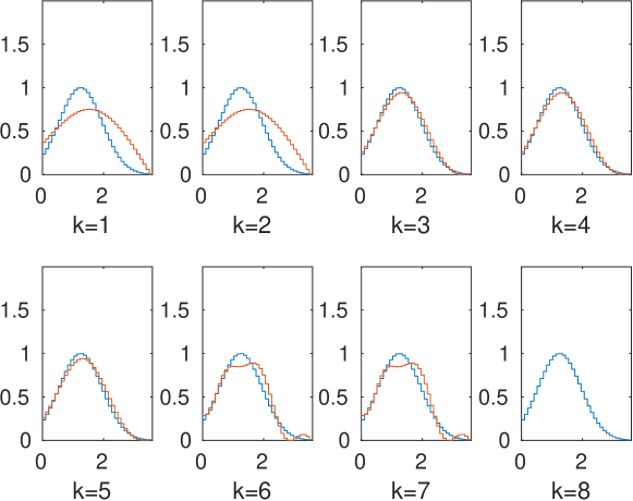
Figure 1: Regularized solutions computed by a call to driver, compared to the exact solution which generated the synthetic data set. The regularization parameter, that is the TGSVD truncation parameter, is denoted by $k$.

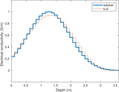
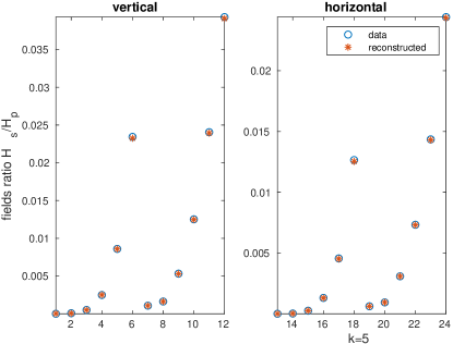
Figure 2: The graph on the left shows the solution selected by the “corner” criterion; the one on the right the data fitting between the synthetic data set and the model prediction. This two graphs can be updated by clicking with the left mouse button on one of the solutions displayed in Figure 1.

The driver program provided with the package generates a synthetic data set corresponding to a device operating with a single pair of coils, at 6 operating frequencies, and a single height above the ground. Both the vertical and the horizontal orientations are considered so that there are $m=12$ data points, but since the complex signal is processed the number of data values to fit is doubled. The subsoil is discretized in $n=35$ equal layers, up to a depth of 3.5m. We assume a constant magnetic permeability $\mu_{0}$ (the value in the empty space) and reconstruct the distribution of the electrical conductivity.

During the computation, information about the data set and the intermediate results are displayed in the MATLAB main window and in some figures, which we reproduce here. Figure 1 shows the regularized solutions computed, while the graph on the left of Figure 2 displays the solution selected by the “corner” criterion, and the one on the right the fitting between the input data set and the model prediction corresponding to the computed solution. We remark that actual calls to driver may produce different results, because different realizations of the noise vector propagate differently in the computation.

A second test program driver2D is provided, which performs the processing of an experimental data set composed by 6 measurements. An additional figure displays the computed solutions in a 2D pseudo-color plot; see Figure 3.

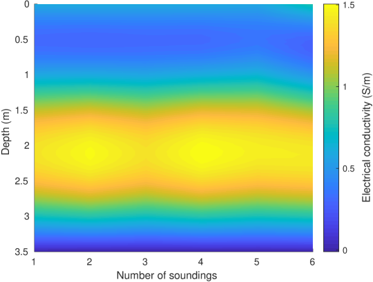
Figure 3: Reconstruction of the electrical conductivity from experimental data, as performed by the driver2D test script.

Table 2 reports the options that can be set to tune the functionality of the package. All the options have a default value; see the driver program for an example of their use, as well as the help pages of the computational routines.

Further information on the use of the package, as well as on the data structure adopted to read experimental data sets, is provided in the User Manual, included in the package main directory.

Table 2: Options for the tuning of the computational routines in the package.

Problem and Data Definition
func	function to be minimized, defaults to aconduct
orientation	orientation of device (vertical, horizontal, or both)
yrows	data rows being processed (useful to exclude some data)
Iterative Method Tuning
sigmainit	starting vector for conductivity sigma (emsolvenlsig)
mu	estimated value of mu in each layer (emsolvenlsig)
muinit	starting vector for permeability mu (emsolvenlmu)
sigma	estimated value of sigma in each layer (emsolvenlmu)
tau	stop tolerance
nmax	maximum number of iterations
damped	set to 1 for damped method, to 0 for undamped
dampos	set to 1 for positive solution, to 0 for unconstrained
metjac	method to compute/approximate the Jacobian
kbroyden	interval for Broyden’s Jacobian updates (see [9])
Regularization Matrix and Parameter Estimation
Lind	index of regularization matrix ($k$th derivative)
metk	methods for choosing the regularization parameter
ds	standard deviation of noise for discrepancy principle
taudiscr	$\tau$ factor for discrepancy principle
Displaying Intermediate Results
show	if $>0$ show information on iterations
showpar	if $>0$ show information on identification of reg. parameter
rowcol	size of grid in the iteration graphical window
xlim	x-limit for the graphs in the iteration window
ylim	y-limit for the graphs in the iteration window
truesol	exact solution, if available (to compute errors)

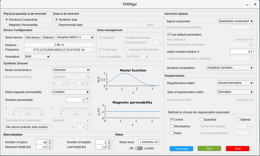
Figure 4: The FDEMgui graphical user interface.

While for processing large experimental data sets it is probably preferable to use a script resembling the driver program, the toolbox includes a MATLAB graphical user interface (GUI) in order to simplify experimenting with the functions of the package. It is started by issuing the command FDEMgui in the main MATLAB window; see Figure 4. It is composed of a set of input panels that lets the user generate or load data sets, choose different approaches and parameters for the inversion algorithm and, finally, visualize the computed results. The panels, which are extensively described in the User Manual, are the following:

• Physical quantity to be inverted,

• Data to be inverted,

• Device configuration,

• Data management,

• Synthetic dataset,

• Discretization,

• Noise,

• Inversion options,

• Regularization.

The GUI is completed by three buttons that allow the user to start the computation, interrupt it, in case something goes wrong, and save the computed solution to a .mat file.

4 Conclusions

In this paper we presented a new MATLAB toolbox for reconstructing the electromagnetic features of the subsoil starting from FDEM data sets, by a regularized, damped, Gauss–Newton method. The package has been developed and extensively tested in various papers recently published. The toolbox includes both test programs, that demonstrates its use, and a graphical user interface, which simplifies setting the parameters that control the package functions.

References

- [1] Anderson, W.L.: Numerical integration of related Hankel transforms of orders 0 and 1 by adaptive digital filtering. Geophysics 44(7), 1287–1305 (1979)
- [2] Björck, Å.: Numerical Methods for Least Squares Problems. SIAM, Philadelphia (1996)
- [3] Boaga, J., Ghinassi, M., D’Alpaos, A., Deidda, G.P, Rodriguez, G., Cassiani, G.: Geophysical investigations unravel the vestiges of ancient meandering channels and their dynamics in tidal landscapes. Sci. Rep. 8, 1708 (8 pages) (2018)
- [4] Borchers, B., Uram, T., Hendrickx, J.: Tikhonov regularization of electrical conductivity depth profiles in field soils. Soil Sci. Soc. Am. J. 61(4), 1004–1009 (1997)
- [5] Cassiani, G., Ursino, N., Deiana, R., Vignoli, G., Boaga, J., Rossi, M., Perri, M.T., Blaschek, M., Duttmann, R., Meyer, S., Ludwig, R., Soddu, A., Dietrich, P., Werban, U.: Noninvasive monitoring of soil static characteristics and dynamic states: a case study highlighting vegetation effects on agricultural land. Vadose Zone J. 11(13) (2012)
- [6] Deidda, G.P, Díaz de Alba, P., Rodriguez, G.: Identifying the magnetic permeability in multi-frequency EM data inversion. Electron. Trans. Numer. Anal. 47, 1–17 (2017)
- [7] Deidda, G.P., Díaz de Alba, P., Rodriguez, G., Vignoli, G.: Smooth and sparse inversion of EMI data from multi-configuration measurements. In: 2018 IEEE 4th International Forum on Research and Technology for Society and Industry (RTSI) (RTSI 2018), pp. 213–218. Palermo, Italy (2018)
- [8] Deidda, G.P., Díaz de Alba, P., Rodriguez, G., Vignoli, G.: Inversion of multi-configuration complex EMI data with minimum gradient support regularization (2019). \htmladdnormallinkarXiv:1904.04563 [math.NA]https://arxiv.org/abs/1904.04563
- [9] Deidda, G.P., Fenu, C., Rodriguez, G.: Regularized solution of a nonlinear problem in electromagnetic sounding. Inverse Problems 30, 125014 (27 pages) (2014)
- [10] Díaz de Alba, P., Fermo, L., van der Mee, C., Rodriguez, G.: Recovering the electrical conductivity of the soil via a linear integral model. J. Comput. Appl. Math. 352, 132–145 (2019)
- [11] Díaz de Alba, P., Rodriguez, G.: Regularized inversion of multi-frequency EM data in geophysical applications. In: F. Ortegón Gallego, M. Redondo Neble, J. Rodríguez Galván (eds.) Trends in Differential Equations and Applications, SEMA SIMAI Springer Series, vol. 8, pp. 357–369. Springer, Switzerland (2016)
- [12] Dragonetti, G., Comegna, A., Ajeel, A., Deidda, G.P, Lamaddalena, N., Rodriguez, G., Vignoli, G., Coppola, A.: Calibrating electromagnetic induction conductivities with time-domain reflectometry measurements. Hydrol. Earth. Syst. Sc. 22, 1509–1523 (2018)
- [13] Golub, G.H., Van Loan, C.F.: Matrix Computations, third edn. The John Hopkins University Press, Baltimore (1996)
- [14] Hansen, P., Jensen, T., Rodriguez, G.: An adaptive pruning algorithm for the discrete L-curve criterion. J. Comput. Appl. Math. 198(2), 483–492 (2007)
- [15] Hansen, P.C.: Rank–Deficient and Discrete Ill–Posed Problems. SIAM, Philadelphia (1998)
- [16] Hansen, P.C.: Regularization Tools: version 4.0 for Matlab 7.3. Numer. Algorithms 46, 189–194 (2007)
- [17] Hendrickx, J.M.H., Borchers, B., Corwin, D.L., Lesch, S.M., Hilgendorf, A.C., Schlue, J.: Inversion of soil conductivity profiles from electromagnetic induction measurements. Soil Sci. Soc. Am. J. 66(3), 673–685 (2002). Package NONLINEM38 available at http://infohost.nmt.edu/~borchers/nonlinem38.html
- [18] Hendrickx, J.M.H., Borchers, B., Corwin, D.L., Lesch, S.M., Hilgendorf, A.C., Schlue, J.: Inversion of soil conductivity profiles from electromagnetic induction measurements: Theory and experimental verification. Soil Sci. Soc. Am. J. 66(3), 673–685 (2002)
- [19] Hochstenbach, M.E., Reichel, L., Rodriguez, G.: Regularization parameter determination for discrete ill-posed problems. J. Comput. Appl. Math. 273, 132–149 (2015)
- [20] Huang, H., SanFilipo, B., Oren, A., Won, I.J.: Coaxial coil towed EMI sensor array for uxo detection and characterization. J. Appl. Geophys. 61(3), 217–226 (2007)
- [21] Lascano, E., Martinelli, P., Osella, A.: EMI data from an archaeological resistive target revisited. Near Surf. Geophy. 4(6), 395–400 (2006)
- [22] Martinelli, P., Duplaá, M.C.: Laterally filtered 1D inversions of small-loop, frequency-domain EMI data from a chemical waste site. Geophysics 73(4), F143–F149 (2008)
- [23] McNeill, J.D.: Electromagnetic terrain conductivity measurement at low induction numbers. Technical Report TN-6 Geonics Limited (1980)
- [24] Morigi, S., Reichel, L., Sgallari, F., Zama, F.: Iterative methods for ill-posed problems and semiconvergent sequences. J. Comput. Appl. Math. 193(1), 157–167 (2006)
- [25] Morozov, V.A.: The choice of parameter when solving functional equations by regularization. Doklady Akademii Nauk SSSR 175, 1225–1228 (1962)
- [26] Osella, A., de la Vega, M., Lascano, E.: 3D electrical imaging of an archaeological site using electrical and electromagnetic methods. Geophysics 70(4), G101–G107 (2005)
- [27] Park, Y., Reichel, L., Rodriguez, G., Yu, X.: Parameter determination for Tikhonov regularization problems in general form. J. Comput. Appl. Math. 343, 12–25 (2018)
- [28] Portniaguine, O., Zhdanov, M.: Focusing geophysical inversion images. Geophysics 64, 874–887 (1999)
- [29] Reichel, L., Rodriguez, G.: Old and new parameter choice rules for discrete ill-posed problems. Numer. Algorithms 63(1), 65–87 (2013)
- [30] Vignoli, G., Deiana, R., Cassiani, G.: Focused inversion of Vertical Radar Profile (VRP) travel–time data. Geophysics 77, H9–H18 (2012)
- [31] Vignoli, G., Fiandaca, G., Christiansen, A., Kirkegaard, C., Auken, E.: Sharp spatially constrained inversion with applications to transient electromagnetic data. Geophys. Prospect. 63, 243–255 (2015)
- [32] Wait, J.R.: Geo–Electromagnetism. New York: Academic, New York, NY (1982)
- [33] Ward, S.H., Hohmann, G.W.: Electromagnetic theory for geophysical applications. (In Electromagnetic Methods in Applied Geophysics). Society of Exploration Geophysicists, Tulsa, OK (1987)
- [34] Yao, R., Yang, J.: Quantitative evaluation of soil salinity and its spatial distribution using electromagnetic induction method. Agric. Water Manag. 97(12), 1961–1970 (2010)
- [35] Zhdanov, M.: Geophysical Inverse Theory and Regularization Problems. Elsevier, Amsterdam (2002)
- [36] Zhdanov, M., Vignoli, G., Ueda, T.: Sharp boundary inversion in crosswell travel–time tomography. J. Geophys. Eng. 3, 122–134 (2006)